Measurement-efficient quantum Krylov subspace diagonalisation

Abstract

The Krylov subspace methods, being one category of the most important classical numerical methods for linear algebra problems, their quantum generalisation can be much more powerful. However, quantum Krylov subspace algorithms are prone to errors due to inevitable statistical fluctuations in quantum measurements. To address this problem, we develop a general theoretical framework to analyse the statistical error and measurement cost. Based on the framework, we propose a quantum algorithm to construct the Hamiltonian-power Krylov subspace that can minimise the measurement cost. In our algorithm, the product of power and Gaussian functions of the Hamiltonian is expressed as an integral of the real-time evolution, such that it can be evaluated on a quantum computer. We compare our algorithm with other established quantum Krylov subspace algorithms in solving two prominent examples. It is shown that the measurement number in our algorithm is typically $10^{4}$ to $10^{12}$ times smaller than other algorithms. Such an improvement can be attributed to the reduced cost of composing projectors onto the ground state. These results show that our algorithm is exceptionally robust to statistical fluctuations and promising for practical applications.

I Introduction

Finding the ground-state energy of a quantum system is of vital importance in many fields of physics Dagotto (1994); Wall and Neuhauser (1995); Caurier et al. (2005). The Lanczos algorithm Lanczos (1950); Saad (2011) is one of the most widely used algorithms to solve this problem. It belongs to the Krylov subspace methods Björck (2015), in which the solution usually converges to the true answer with an increasing subspace dimension. However, such methods are unscalable for many-body systems because of the exponentially-growing Hilbert space dimension Avella and Mancini (2013). In quantum computing, there is a family of hybrid quantum-classical algorithms that can be regarded as a quantum generalisation of the classical Lanczos algorithm Motta et al. (2019); Yeter-Aydeniz et al. (2020); Parrish and McMahon ; Stair et al. (2020); Bespalova and Kyriienko (2021); Cohn et al. (2021); Klymko et al. (2022); Cortes and Gray (2022); Epperly et al. (2022); Shen et al. ; Kyriienko (2020); Seki and Yunoki (2021); Kirby et al. . Following Refs. Stair et al. (2020); Cortes and Gray (2022); Epperly et al. (2022), we call them quantum Krylov subspace diagonalisation (KSD). These algorithms are scalable with the system size by carrying out the classically-intractable vector and matrix arithmetic on the quantum computer. They possess potential advantages as the conventional quantum algorithm to solve the ground-state problem, quantum phase estimation, requires considerable quantum resources Babbush et al. (2018); Lee et al. (2021), while the variational quantum eigensolver is limited by the ansatz and classical optimisation bottlenecks Peruzzo et al. (2014); McClean et al. (2018).

However, Krylov subspace methods are often confronted with the obstacle that small errors can cause large deviations in the ground-state energy. This issue is rooted in the Krylov subspace that is spanned by an almost linearly dependent basis Parlett (1998); Householder (2013). Contrary to classical computing, in which one can exponentially suppress rounding errors by increasing the number of bits, quantum computing is inherently subject to statistical error. Since statistical error decreases slowly with the measurement number $M$ as $\propto 1/\sqrt{M}$, an extremely large $M$ can be required to reach an acceptable error. In this case, although quantum KSD algorithms perform well in principle, the measurement cost has to be assessed and optimised for realistic implementations Epperly et al. (2022); Kirby et al. .

In this work, we present a general and rigorous analysis of the measurement cost in quantum KSD algorithms. Specifically, we obtain an upper bound formula of the measurement number that is applicable to all quantum KSD algorithms. Then, we propose an algorithm to construct the Hamiltonian-power Krylov subspace Björck (2015). In our algorithm, we express the product of Hamiltonian power and a Gaussian function of Hamiltonian as an integral of real-time evolution. In this way, the statistical error decreases exponentially with the power, which makes our algorithm measurement-efficient. We benchmark quantum KSD algorithms by estimating their measurement costs in solving the anti-ferromagnetic Heisenberg model and the Hubbard model. Various lattices of each model are taken in the benchmarking. We find that typically our algorithm requires $10^{4}$ to $10^{12}$ times fewer measurements in comparison with others.

II Krylov subspace diagonalisation

First, we introduce the KSD algorithm and some relevant notations. The algorithm starts with a reference state $|{\varphi}\rangle$. Then we generate a set of basis states $|{\phi_{k}}\rangle=f_{k}(H)|{\varphi}\rangle$, where $H$ is the Hamiltonian, and $f_{1},f_{2},\ldots,f_{d}$ are linearly-independent $(d-1)$-degree polynomials (to generate a $d$-dimensional Krylov subspace). For example, it is conventional to take the power function $f_{k}(H)=H^{k-1}$ in the Lanczos algorithm. These states span a subspace called the Krylov subspace. We compute the ground-state energy by solving the generalised eigenvalue problem $\mathbf{H}\mathbf{a}=E\mathbf{S}\mathbf{a}$, where $\mathbf{H}_{k,q}=\langle{\phi_{k}}|H|{\phi_{q}}\rangle$ and $\mathbf{S}_{k,q}=\langle\phi_{k}|\phi_{q}\rangle$. Let $E_{min}$ be the minimum eigenvalue of the generalised eigenvalue problem. The error in the ground-state energy is $\epsilon_{K}=E_{min}-E_{g}$, where $E_{g}$ is the true ground-state energy. We call $\epsilon_{K}$ the subspace error. One can also construct generalised Krylov subspaces in which $f_{k}$ are functions of $H$ other than polynomials; see Table 1.

In the literature, subspaces generated by variational quantum circuits McClean et al. (2017); Parrish et al. (2019); Nakanishi et al. (2019); Huggins et al. (2020) and stochastic time evolution Stair et al. are also proposed. Quantum KSD techniques can also be used to mitigate errors caused by imperfect gates McClean et al. (2017, 2020); Yoshioka et al. (2022). In this work, we focus on Hamiltonian functions because of their similarities to conventional Krylov subspace methods.

Abbr.	$f_{k}(x)$	Refs.
P	$x^{k-1}$	Seki and Yunoki (2021); Bespalova and Kyriienko (2021)
CP	$T_{k-1}(x/h_{tot})$	Kirby et al.
GP	$x^{k-1}e^{-\frac{1}{2}x^{2}\tau^{2}}$	This work
IP	$x^{-(k-1)}$	Kyriienko (2020)
ITE	$e^{-\tau(k-1)x}$	Motta et al. (2019); Yeter-Aydeniz et al. (2020)
RTE	$e^{-ix\Delta t\left(k-\frac{d+1}{2}\right)}$	Parrish and McMahon ; Stair et al. (2020); Bespalova and Kyriienko (2021); Cohn et al. (2021); Klymko et al. (2022); Cortes and Gray (2022); Epperly et al. (2022); Shen et al.
F	$L^{-1}\sum_{l=1}^{L}e^{-i\left[x-\Delta E\left(k-1\right)\right]\Delta t\left(l-\frac{L+1}{2}\right)}$	Cortes and Gray (2022)

Table 1: Operators $f_{k}(x)$ generating the basis of a (generalised) Krylov subspace. Here $x=H-E_{0}$, where $E_{0}$ is a constant. In different algorithms, $f_{k}$ can be power (P), Chebyshev polynomial (CP), Gaussian-power (GP), inverse power (IP) or exponential [i.e. imaginary-time evolution (ITE), real-time evolution (RTE) and filter (F)] functions of the Hamiltonian. $T_{n}$ is the $n$-th Chebyshev polynomial of the first kind, and $E_{0}=0$ in the CP basis. For a Hamiltonian expressed in the form $H=\sum_{j}h_{j}\sigma_{j}$, where $\sigma_{j}$ are Pauli operators, $h_{tot}=\sum_{j}|h_{j}|$ is the 1-norm of coefficients. $\tau$, $\Delta t$ and $\Delta E$ are some real parameters.

III General analysis of the measurement cost

In addition to $\epsilon_{K}$, the other error source is the statistical error. In quantum KSD algorithms, matrices $\mathbf{H}$ and $\mathbf{S}$ are obtained by measuring qubits at the end of certain quantum circuits. In this work, we rigorously analyse the number of measurements required for achieving a given permissible total error $\epsilon$ (including both $\epsilon_{K}$ and statistical error). We divide the measurement number into three factors. The first two factors are the same for different bases of Krylov subspaces, and the third factor depends on the basis (i.e. $f_{k}$ operators in Table 1). In this work, we show that the third factor is drastically reduced in our measurement-efficient algorithm.

The total measurement number required for implementing a quantum KSD algorithm consists of three factors,

$$M_{tot}=\frac{\alpha(\kappa)\|H\|_{2}^{2}}{p_{g}^{2}\epsilon^{2}}\times\beta(d)\times\gamma.$$ (1)

The first factor is the cost of measuring the energy. Roughly speaking, it is the cost in the ideal case that one can prepare the ground state by an ideal projection; see Appendix A. The spectral norm $\|H\|_{2}$ characterises the range of the energy. Assume that the statistical error and $\epsilon$ are comparable, $M_{tot}\propto\|H\|_{2}^{2}/\epsilon^{2}$ according to the standard scaling of the statistical error. $\kappa$ is the permissible failure probability: The actual error may exceed $\epsilon$ due to the statistical error, and $\alpha(\kappa)$ is the overhead for achieving the probability. We take $\alpha(\kappa)=256/\kappa$ in the rigorous bound analysis, although $\alpha(\kappa)\approx 16\ln(1/\kappa)$ is sufficient in practice; see Appendix B. The success of KSD algorithms depends on a finite overlap between the reference state and the true ground state $|{\psi_{g}}\rangle$ Björck (2015); Epperly et al. (2022); Kirby et al. . This requirement is reflected in $M_{tot}\propto 1/p_{g}^{2}$, where $p_{g}=|\langle\psi_{g}|\varphi\rangle|^{2}$. The second factor, $\beta(d)$, is the overhead due to measuring $d\times d$ matrices. There are more sources of statistical errors (matrix entries) influencing the eventual result when $d$ is larger. We take $\beta(d)=d^{6}$ in the rigorous bound analysis, and it can be reduced to $\beta(d)=d(2d-1)$ after optimisation; see Appendix B. The remaining factor $\gamma$ depends on the spectrum of $\mathbf{S}$ (i.e. the basis), as we will show later. In the numerical result, we find that the typical value of $\gamma$ in quantum KSD algorithms can be as large as $10^{12}$ to achieve certain $\epsilon$, and our algorithm reduces $\gamma$ to about $3$.

1:

2:Input $\hat{H}$, $\hat{S}$, $C_{\mathbf{H}}$, $C_{\mathbf{S}}$ and $\eta>0$.

3:Solve the generalised eigenvalue problem

$$(\hat{\mathbf{H}}+C_{\mathbf{H}}\eta)\mathbf{a}=E(\hat{\mathbf{S}}+C_{\mathbf{S}}\eta)\mathbf{a}$$

4:Output the minimum eigenvalue $\hat{E}_{min}$.

Algorithm 1 Regularised quantum Krylov-subspace diagonalisation algorithm.

IV Rigorous bound of the measurement cost

For a rigorous bound analysis, we assume that each matrix entry is measured individually. In Appendix B, we give a better setup for the practical implementation. The budget for each matrix entry is $2M$ measurements [i.e. $M=M_{tot}/(4d^{2})$]. Notice that the entry is complex and has two parts in general, and the budget for each part is $M$. Measurements yield estimators $\hat{\mathbf{H}}$ and $\hat{\mathbf{S}}$ of two matrices. Variances of estimators have upper bounds in the form $\mathrm{Var}(\hat{\mathbf{H}}_{k,q})\leqslant 2C_{\mathbf{H}}^{2}/M$ and $\mathrm{Var}(\hat{\mathbf{S}}_{k,q})\leqslant 2C_{\mathbf{S}}^{2}/M$, where $C_{\mathbf{H}}$ and $C_{\mathbf{S}}$ are some factors depending on the protocol. Let $\hat{E}_{min}$ be the minimum eigenvalue computed using $\hat{\mathbf{H}}$ and $\hat{\mathbf{S}}$ (see Algorithm 1). The total error is $|\hat{E}_{min}-E_{g}|$, and the computing succeeds when $|\hat{E}_{min}-E_{g}|\leqslant\epsilon$. If estimators are unbiased, $\hat{E}_{min}\rightarrow E_{min}$ in the limit $M_{tot}\rightarrow+\infty$. Therefore, we can achieve any permissible error $\epsilon>\epsilon_{K}$ with some sufficiently large $M_{tot}$. The first result of this work is about the sufficiently large $M_{tot}$, which is summarised in the following theorem.

Theorem 1.

Suppose $\epsilon>\epsilon_{K}$ and $E_{g}+\epsilon<0$. The total measurement number in Eq. (1) with $\alpha(\kappa)=256/\kappa$, $\beta(d)=d^{6}$ and

$$\gamma=\frac{p_{g}^{2}\epsilon^{2}}{16\|H\|_{2}^{2}\eta^{2}}$$ (2)

is sufficient for achieving the permissible error $\epsilon$ and failure probability $\kappa$, i.e. $\hat{E}_{min}\in[E_{g},E_{g}+\epsilon]$ with a probability of at least $1-\kappa$. Here $\eta$ is the solution to the equation $\min_{\mathbf{a}\neq 0}E^{\prime}(\eta,\mathbf{a})=E_{g}+\epsilon$, and

$$E^{\prime}(\eta,\mathbf{a})=\frac{\mathbf{a}^{\dagger}(\mathbf{H}+2C_{\mathbf{H}}\eta)\mathbf{a}}{\mathbf{a}^{\dagger}(\mathbf{S}+2C_{\mathbf{S}}\eta)\mathbf{a}}.$$ (3)

See Appendix A for the proof. About the condition $E_{g}+\epsilon<0$, notice that we can always subtract a positive constant from the Hamiltonian to satisfy this condition.

The measurement overhead $\gamma$ depends on the spectrum of $\mathbf{S}$. Let’s consider a small $\eta$ and the Taylor expansion of $E^{\prime}$. The minimum value of the zeroth-order term $\frac{\mathbf{a}^{\dagger}\mathbf{H}\mathbf{a}}{\mathbf{a}^{\dagger}\mathbf{S}\mathbf{a}}$ is $E_{min}$ according to the Rayleigh quotient theorem Horn and Johnson (2012). Take this minimum value, we have $E^{\prime}\simeq E_{min}+s\eta$, where $s\propto\frac{\mathbf{a}^{\dagger}\mathbf{a}}{\mathbf{a}^{\dagger}\mathbf{S}\mathbf{a}}$ is the first derivative. The solution to $E^{\prime}=E_{g}+\epsilon$ is $\eta\simeq(E_{g}+\epsilon-E_{min})/s$, then $\gamma\simeq u^{2}\left(\frac{p_{g}\mathbf{a}^{\dagger}\mathbf{a}}{\mathbf{a}^{\dagger}\mathbf{S}\mathbf{a}}\right)^{2}$, where $u\leqslant\frac{(C_{\mathbf{H}}+\|H\|_{2}C_{\mathbf{S}})\epsilon}{2\|H\|_{2}(\epsilon-\epsilon_{K})}\approx C_{\mathbf{S}}$ under assumptions $C_{\mathbf{H}}\approx\|H\|_{2}C_{\mathbf{S}}$ and $\epsilon-\epsilon_{K}\approx\epsilon$. Therefore, when $\mathbf{S}$ is close to singular, the overhead can be large.

In the above analysis, we add a positive diagonal matrix to $\hat{\mathbf{S}}$ to overcome the problem caused by an ill-conditioned $\mathbf{S}$ (see Algorithm 1 and Appendix A). There is an alternative approach called thresholding procedure Motta et al. (2019); Epperly et al. (2022) dealing with the same problem, based on which the asymptotic behaviour of $M$ is provided Kirby et al. .

V Measurement-efficient algorithm

As we have shown, the measurement overhead $\gamma$ depends on the overlap matrix $\mathbf{S}$, i.e. how we choose the basis of Krylov subspace. The main advantage of our algorithm is that we utilise a basis resulting in a small $\gamma$.

To generate a standard Krylov subspace, we choose operators

$$f_{k}=(H-E_{0})^{k-1}e^{-\frac{1}{2}(H-E_{0})^{2}\tau^{2}},$$ (4)

where $E_{0}$ is a constant up to choice. We call it the Gaussian-power basis. The corresponding subspace is a conventional Hamiltonian-power Krylov subspace, but the reference state $|{\varphi}\rangle$ has been effectively replaced by $e^{-\frac{1}{2}(H-E_{0})^{2}\tau^{2}}|{\varphi}\rangle$.

A property of the Gaussian-power basis is that the spectral norm $\|f_{k}\|_{2}\leqslant(\frac{k-1}{e\tau^{2}})^{\frac{k-1}{2}}\leqslant(\frac{d-1}{e\tau^{2}})^{\frac{k-1}{2}}$ has an upper bound decreasing exponentially with $k$, under the condition $e\tau^{2}>d-1$. Here, $e$ is Euler’s constant. This property is essential for the measurement efficiency of our algorithm.

We propose to realise the Gaussian-power basis by expressing the operator of interest as a linear combination of unitaries (LCU). The same approach has been taken to realise other bases like power Seki and Yunoki (2021); Bespalova and Kyriienko (2021), inverse power Kyriienko (2020), imaginary-time evolution Huo and Li (2023), filter Cortes and Gray (2022) and Gaussian function of the Hamiltonian Zeng et al. .

Suppose we want to measure the quantity $\langle{\varphi}|A|{\varphi}\rangle$. Here $A=f_{k}^{\dagger}Hf_{q}$ and $A=f_{k}^{\dagger}f_{q}$ for $\mathbf{H}_{k,q}$ and $\mathbf{S}_{k,q}$, respectively. First, we work out an expression in the from $A=\sum_{s}q_{s}U_{s}$, where $U_{s}$ are unitary operators, and $q_{s}$ are complex coefficients. Then, there are two ways to measure $\langle{\varphi}|A|{\varphi}\rangle$. When the expression has finite terms, we can apply $A$ on the state $|{\varphi}\rangle$ by using a set of ancilla qubits; In the literature, LCU usually refers to this approach Childs and Wiebe (2012). Alternatively, we can individually measure each term $\langle{\varphi}|U_{s}|{\varphi}\rangle$ with the Hadamard-test circuit Ekert et al. (2002) and compute the summation $\langle{\varphi}|A|{\varphi}\rangle$ using the Monte Carlo method Faehrmann et al. (2022). The second way works for an expression with even infinite terms and requires only one or zero ancilla qubits O’Brien et al. (2021); Lu et al. (2021). We focus on the Monte Carlo method in this work.

Now we give our LCU expression. Suppose we already express $H$ as a linear combination of Pauli operators, it is straightforward to work out the LCU expression of $A$ given the expression of $f_{k}$. Therefore, we only give the expression of $f_{k}$. Utilising the Fourier transformation of a modified Hermite function (which is proved in Appendix C), we can express $f_{k}$ in Eq. (4) as

$$f_{k}=\frac{i^{k-1}}{2^{\frac{k-1}{2}}\tau^{k-1}}\int_{-\infty}^{+\infty}dtH_{k-1}\left(\frac{t}{\sqrt{2}\tau}\right)g_{\tau}(t)e^{-ixt},$$ (5)

where $H_{n}(u)$ denotes Hermite polynomials, $g_{\tau}(t)=\frac{1}{\tau\sqrt{2\pi}}e^{-\frac{t^{2}}{2\tau^{2}}}$ is the normalised Gaussian function, $x=H-E_{0}$, and $e^{-ixt}$ is the real-time evolution (RTE) operator.

VI Real time evolution

There are various protocols for implementing RTE, including Trotterisation Lloyd (1996); Berry et al. (2007); Wiebe et al. (2010), LCU Childs and Wiebe (2012); Berry et al. (2015); Meister et al. (2022); Faehrmann et al. (2022) and qDRIFT Campbell (2019), etc. In most of the protocols, RTE is inexact but approaches the exact one when the circuit depth increases. Therefore, all these protocols work for our algorithm as long as the circuit is sufficiently deep. In this work, we specifically consider an LCU-type protocol, the zeroth-order leading-order-rotation formula Yang et al. (2021).

In the leading-order-rotation protocol, RTE is exact even when the circuit depth is finite. In this protocol, we express RTE in the LCU form $e^{-iHt}=\left[\sum_{r}v_{r}(t/N)V_{r}(t/N)\right]^{N}$, where $V_{r}(t)=e^{-i\phi(t)\sigma},\sigma$ is a rotation or Pauli operator, $v_{r}(t)$ are complex coefficients, and $N$ is the time step number. This exact expression of RTE is worked out in the spirit of Taylor expansion and contains infinite terms. Notice that $N$ determines the circuit depth. See Appendix D for details. Substituting the expression of $e^{-iHt}$ into Eq. (5), we obtain the eventual LCU expression of $f_{k}$.

VII Bias and variance

Let $\hat{A}$ be the estimator of $\langle{\varphi}|A|{\varphi}\rangle$. There are two types of errors in $\hat{A}$, bias and variance. Because RTE is exact in the leading-order-rotation protocol, the estimator $\hat{A}$ is unbiased. Therefore, we can focus on the variance from now on.

If we use the Monte Carlo method and the one-ancilla Hadamard test to evaluate the LCU expression of $A$, the variance has the upper bound

$$\mathrm{Var}(\hat{A})\leqslant\frac{2C_{A}^{2}}{M},$$ (6)

where $2M$ is the measurement number, and $C_{A}=\sum_{s}|q_{s}|$ is the 1-norm of coefficients in the expression. We call $C_{A}$ the cost of the LCU expression. We remark that the variance in this form is universal and valid for all algorithms with some proper factor $C_{A}$.

The cost of an LCU expression is related to the spectral norm. Notice $\|U_{s}\|_{2}=1$, we immediately conclude that $C_{A}\geqslant\|A\|_{2}$. Therefore, when $\|f_{k}\|_{2}$ decreases exponentially with $k$, it is possible to measure $\langle{\varphi}|A|{\varphi}\rangle$ with an error decreasing exponentially with $k$.

In our algorithm, we find that the cost has the form

$$C_{A}=h_{tot}c_{k}c_{q}\text{ and }c_{k}c_{q}$$ (7)

for $\mathbf{H}_{k,q}$ and $\mathbf{S}_{k,q}$, respectively. $c_{k}$ is the cost due to $f_{k}$, and

$$c_{k} = \frac{1}{2^{\frac{k-1}{2}}\tau^{k-1}}\int_{-\infty}^{+\infty}dt\left|H_{k-1}\left(\frac{t}{\sqrt{2}\tau}\right)\right|g_{\tau}(t)$$ (8)

$$\times\left[\sum_{r}\left|v_{r}\left(\frac{t}{N}\right)\right|\right]^{N}\leqslant 2\left(\frac{k-1}{e\tau^{2}}\right)^{\frac{k-1}{2}}.$$

Here, we have taken the time step number $N=4eh_{tot}^{2}\tau^{2}$ to work out the upper bound. We can find that we already approach the lower bound of the variance given by the spectral norm (The difference is a factor of $2$). As a result, the variance of $\hat{A}$ decreases exponentially with $k$ and $q$.

Detailed pseudocodes and analysis are given in Appendix D. There are two ways to apply Theorem 1: First, we can take $C_{\mathbf{H}}=h_{tot}C_{\mathbf{S}}$ and $C_{\mathbf{S}}=\max\{c_{k}c_{q}\}$; Second, we can rescale the basis by taking $f^{\prime}_{k}=f_{k}/c_{k}$. Matrix entries $\hat{\mathbf{H}}^{\prime}_{k,q}$ and $\hat{\mathbf{S}}^{\prime}_{k,q}$ of the rescaled basis $\{f^{\prime}_{k}|{\varphi}\rangle\}$ have variance upper bounds $2h_{tot}^{2}/M$ and $2/M$, respectively. Therefore, $C_{\mathbf{H}}=h_{tot}$ and $C_{\mathbf{S}}=1$ for the rescaled basis. We take the rescaled basis in the numerical study.

VIII Measurement overhead benchmarking

We benchmark the measurement cost in quantum KSD algorithms listed in Table 1. Two models of strongly correlated systems, namely, the anti-ferromagnetic Heisenberg model and Hubbard model Anderson (1987); Lee et al. (2006); Avella and Mancini (2013); Seki et al. (2020), are used in benchmarking. For each model, the lattice is taken from two categories: regular lattices, including chain and ladder, and randomly generated graphs. We fix the lattice size such that the Hamiltonian can be encoded into ten qubits. For each Hamiltonian specified by the model and lattice, we evaluate all quantum KSD algorithms with the same subspace dimension $d$ taken from $2,3,\ldots,30$. In total, $257$ instances of $(model,lattice,d)$ are generated to benchmark quantum KSD algorithms.

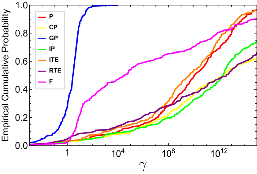
Figure 1: Empirical distribution of the measurement overhead $\gamma$ for algorithms listed in Table 1. In the Gaussian-power algorithm, we take a random $E_{0}$ in the interval $[E_{g}-0.1\|H\|_{2},E_{g}+0.1\|H\|_{2}]$, i.e. we assume that we have a preliminary estimation of the ground-state energy with an uncertainty as large as $10\%$ of the entire spectrum. Details of the numerical calculation are given in Appendix E.

We choose the power algorithm as the standard for comparison. We remark that the power algorithm and the classical Lanczos algorithm yield the same result when the implementation is error-free (i.e. without statistical error and rounding error), and the eventual error in this ideal case is the subspace error $\epsilon_{K}$. Given the model, lattice and subspace dimension, we compute $\epsilon_{K}$ of the power algorithm. Then, we take the permissible error $\epsilon=2\epsilon_{K}$ and compute the overhead factor $\gamma$ for each algorithm. The empirical distribution of $\gamma$ is illustrated in Fig. 1.

From the distribution, we can find that our Gaussian-power algorithm has the smallest measurement overhead, and $\gamma$ is smaller than $10^{2}$ for almost all instances. The filter algorithm is the most well-performed one among others. Part of the reason is that we have taken the optimal $\Delta E$ found by grid search. The median value of $\gamma$ is about $3$ for our Gaussian-power algorithm, $3\times 10^{4}$ for the filter algorithm and as large as $10^{12}$ for some other algorithms.

IX Composing a projector

We can explain the measurement efficiency of our algorithm by composing a projector. In our algorithm with the rescaled basis, the solution is a state in the form $|{\Psi(\mathbf{a})}\rangle=\sum_{k=1}^{d}a_{k}c_{k}^{-1}f_{k}|{\varphi}\rangle$. Ideally, the linear combination of $f_{k}$ realises a projector onto the ground state, i.e. $\sum_{k=1}^{d}a_{k}c_{k}^{-1}f_{k}=|\psi_{g}\rangle\langle\psi_{g}|$. Then, $|{\Psi(\mathbf{a})}\rangle=\sqrt{p_{g}}|{\psi_{g}}\rangle$ up to a phase and $\mathbf{a}^{\dagger}\mathbf{S}\mathbf{a}=\langle\Psi(\mathbf{a})|\Psi(\mathbf{a})\rangle=p_{g}$. Recall $\gamma\approx\left(\frac{p_{g}\mathbf{a}^{\dagger}\mathbf{a}}{\mathbf{a}^{\dagger}\mathbf{S}\mathbf{a}}\right)^{2}=\left(\mathbf{a}^{\dagger}\mathbf{a}\right)^{2}$ (notice that $C_{\mathbf{S}}=1$), we can find that $\mathbf{a}^{\dagger}\mathbf{a}$ determines $\gamma$. When $c_{k}$ is smaller, $|a_{k}|$ required for composing the projector is smaller. In our algorithm, $c_{k}$ decreases exponentially with $k$, and the speed of decreasing is controllable via the parameter $\tau$. In this way, our algorithm results in a small $\gamma$.

To be concrete, let’s consider a classic way of composing a projector from Hamiltonian powers using Chebyshev polynomials $T_{n}$, which has been used for proving the convergence of the Lanczos algorithm Dahlquist and Björck (2008). Without loss of generality, we suppose $\|H\|_{2}=1$. An approximate projector in the form of Chebyshev polynomials is

$$\frac{T_{n}(Z)}{T_{n}(z_{1})}=|\psi_{g}\rangle\langle\psi_{g}|+\Omega,$$ (9)

where $Z=1-(H-E_{g}-\Delta)$, $\Delta$ is the energy gap between the ground state and the first excited state, $z_{1}=1+\Delta$, and $\Omega$ is an operator with the upper bound $\|\Omega\|_{2}\leqslant 2/(z_{1}^{n}+z_{1}^{-n})$. Notice that the error $\Omega$ depends on $n$, and its upper bound decreases exponentially with $n$ if $\Delta$ is finite. For simplicity, we focus on the case that $E_{0}=E_{g}$ in the Hamiltonian power. Then, in the expansion $T_{n}(Z)=\sum_{l=0}^{n}b_{l}(H-E_{g})^{l}$, coefficients have upper bounds $|b_{l}|\leqslant n^{l}T_{n}(z_{1})$ increasing exponentially with $l$. See Appendix F. In the LCU and Monte Carlo approach, large coefficients lead to large variance. Therefore, it is difficult to realise this projector because of the exponentially increasing coefficients.

In our algorithm, the exponentially decreasing $c_{k}$ can cancel out the large $b_{l}$. We can compose the Chebyshev-polynomial projector with an additional Gaussian factor. Taking $d=n+1$ and $a_{k}=c_{k}b_{k-1}/T_{n}(z_{1})$, we have $\sum_{k=1}^{d}a_{k}c_{k}^{-1}f_{k}=\frac{T_{n}(Z)}{T_{n}(z_{1})}e^{-\frac{1}{2}(H-E_{g})^{2}\tau^{2}}$. Because the Gaussian factor is also a projector onto the ground state, the overall operator is a projector with a smaller error than the Chebyshev-polynomial projector. The corresponding overhead factor is

$$\gamma\lesssim 4\frac{1}{1-n^{3}/(e\tau^{2})}.$$ (10)

When $\tau$ is sufficiently large, $\gamma\lesssim 4$. This example shows that the Gaussian-power basis can compose a projector with a small measurement cost.

X Conclusions

In this work, we have proposed a regularised estimator of the ground-state energy (see Algorithm 1). Even in the presence of statistical errors, the regularised estimator is variational (i.e. equal to or above the true ground-state energy) and has a rigorous upper bound. Because of these properties, it provides a universal way of analysing the measurement cost in quantum KSD algorithms, with the result summarised in Theorem 1. This approach can be generalised to analyse the effect of other errors, e.g. imperfect quantum gates. The robustness to statistical errors in our algorithm implies the robustness to other errors.

To minimise the measurement cost, we have proposed a protocol for constructing Hamiltonian power with an additional Gaussian factor. This Gaussian factor is important because it leads to the statistical error decreasing exponentially with the power. Then, we benchmark quantum KSD algorithms with two models of quantum many-body systems. We find that our algorithm requires the smallest measurement number, and a measurement overhead $\gamma$ of a hundred is almost always sufficient for approaching the theoretical-limit accuracy $\epsilon_{K}$ of the Lanczos algorithm. In addition to the advantage over the classical Lanczos algorithm in scalability, our result suggests that the quantum algorithm is also competitive in accuracy at a reasonable measurement cost.

Appendix A Proof of Theorem 1

In this section, we briefly overview the KSD algorithm and then give the proof of Theorem 1.

A.1 General formalism of KSD algorithm

Given a reference state $|{\varphi}\rangle$, a Hamiltonian $H$ and an integer $d$, the standard Krylov subspace is $\mathcal{K}=\mathrm{Span}\left(|{\varphi}\rangle,H|{\varphi}\rangle,H^{2}|{\varphi}\rangle,\ldots,H^{d-1}|{\varphi}\rangle\right)$. This can be seen as taking polynomials $f_{k}(x)=x^{k-1}$. The subspace is the same when $\{f_{1},f_{2},\ldots,f_{d}\}$ is an arbitrary set of linearly-independent $(d-1)$-degree polynomials. Any state in the Krylov subspace can be expressed as

$$|{\psi_{K}}\rangle = \sum_{k=1}^{d}a_{k}f_{k}(H)|{\varphi}\rangle.$$ (11)

The state that minimises the Rayleigh quotient $\langle\psi_{K}|H|\psi_{K}\rangle/\langle\psi_{K}|\psi_{K}\rangle$ is regarded as the approximate ground state of the Hamiltonian $H$, and the corresponding energy is the approximate ground-state energy, i.e.

$$|{\psi_{g}}\rangle \sim |{\psi_{min}}\rangle=\operatorname*{arg\,min}_{\psi_{K}\in\mathcal{K}}\frac{\langle\psi_{K}|H|\psi_{K}\rangle}{\langle\psi_{K}|\psi_{K}\rangle},$$ (12)

$$E_{g} \sim E_{min}=\min_{\psi_{K}\in\mathcal{K}}\frac{\langle\psi_{K}|H|\psi_{K}\rangle}{\langle\psi_{K}|\psi_{K}\rangle}.$$ (13)

Definition 1 (Rayleigh quotient).

For any matrix $\mathbf{A}\in\mathbb{C}^{d\times d}$, and any non-zero vector $\mathbf{a}\in\mathbb{C}^{d}$, the Rayleigh quotient is defined as

$$\langle\mathbf{A}\rangle(\mathbf{a}) = \frac{\mathbf{a}^{\dagger}\mathbf{A}\mathbf{a}}{\mathbf{a}^{\dagger}\mathbf{a}}.$$ (14)

The approximate ground state energy can be rewritten as

$$E_{min} = \min_{\mathbf{a}\neq 0}\frac{\mathbf{a}^{\dagger}\mathbf{H}\mathbf{a}}{\mathbf{a}^{\dagger}\mathbf{S}\mathbf{a}}=\min_{\mathbf{a}\neq 0}\frac{\langle\mathbf{H}\rangle(\mathbf{a})}{\langle\mathbf{S}\rangle(\mathbf{a})},$$ (15)

where $\mathbf{H}$ and $\mathbf{S}$ are $d\times d$ Hermitian matrices as defined in the main text.

It can be shown that $H^{k}|{\varphi}\rangle$ converges to the eigenstate with the largest absolute eigenvalue when $k$ increases. The eigenstate is usually the ground state (If not, take $H\leftarrow H-E_{0}$ where $E_{0}$ is a positive constant). Therefore, it is justified to express the ground state as a linear combination of $\{H^{k}|{\varphi}\rangle\}$ as long as $|{\varphi}\rangle$ has a non-zero overlap with the true ground state $|{\psi_{g}}\rangle$. However, the convergence with $k$ causes inherent trouble that basis vectors of the Krylov subspace are nearly linearly dependent, i.e. the overlap matrix $\mathbf{S}$ is nearly singular and has a large condition number. As a result, the denominator of the Rayleigh quotient can be very small, and a tiny error in computing may cause a large deviation of the approximate ground-state energy $E_{min}$.

According to the Rayleigh-Ritz theorem (Rayleigh quotient theorem) Horn and Johnson (2012), the minimisation problem is equivalent to the generalised eigenvalue problem. The generalised eigenvalue problem can be reduced to an eigenvalue problem while the singularity issue remains. For example, one can use the Cholesky decomposition to express $\mathbf{S}$ as the product of an upper-triangular matrix and its conjugate transpose, i.e. $\mathbf{S}=\mathbf{R}^{\dagger}\mathbf{R}$, and the eigenvalue problem becomes $\left(\mathbf{R}^{\dagger}\right)^{-1}\mathbf{H}\mathbf{R}^{-1}(\mathbf{R}\mathbf{a})=E\mathbf{R}\mathbf{a}$. The Cholesky decomposition, however, also requires the matrix $\mathbf{S}$ to be positive-definite. When $\mathbf{S}$ is nearly singular, the Cholesky decomposition is unstable. One way to address the singularity issue is by adding a positive diagonal matrix to $\mathbf{S}$. In this work, we also add a diagonal matrix to $\mathbf{H}$ to ensure that the Rayleigh quotient is variational, i.e. the energy is not lower than the ground-state energy (with a controllable probability). An alternative way to address the singularity issue is the so-called thresholding method, see Refs. Motta et al. (2019); Epperly et al. (2022).

A.2 Measurement cost in quantum KSD

In this section, we develop theoretical tools for analysing the measurement cost in quantum KSD algorithms. The exact values of $\mathbf{H}$ and $\mathbf{S}$ are unknown, and what we have are their approximate matrices $\hat{\mathbf{H}}$ and $\hat{\mathbf{S}}$ computed by the quantum computer. We assume that the quantum computer is fully fault-tolerant, and errors in $\hat{\mathbf{H}}$ and $\hat{\mathbf{S}}$ are due to the statistical fluctuations. Details of computing $\mathbf{H}$ and $\mathbf{S}$ with a quantum computer are given in Appendix D.

Lemma 1.

Let $\kappa$ and $\eta$ be any positive numbers. The inequality

$$\Pr\left(\|\hat{\mathbf{H}}-\mathbf{H}\|_{2}\leqslant C_{\mathbf{H}}\eta\ \rm{and}\ \|\hat{\mathbf{S}}-\mathbf{S}\|_{2}\leqslant C_{\mathbf{S}}\eta\right)$$ (16)

$$\geqslant 1-\kappa$$

holds when $M\geqslant\frac{4d^{4}}{\kappa\eta^{2}}$.

Proof.

Recall the variance upper bounds of $\hat{\mathbf{H}}_{k,q}$ and $\hat{\mathbf{S}}_{k,q}$ given in the main text. When $M\geqslant\frac{4d^{4}}{\kappa\eta^{2}}$,

$$\mathrm{Var}(\hat{\mathbf{H}}_{k,q}) \leqslant \frac{\kappa C_{\mathbf{H}}^{2}\eta^{2}}{2d^{4}},$$ (17)

$$\mathrm{Var}(\hat{\mathbf{S}}_{k,q}) \leqslant \frac{\kappa C_{\mathbf{S}}^{2}\eta^{2}}{2d^{4}}.$$ (18)

According to Chebyshev’s inequality, we have

$$\Pr\left(|\hat{\mathbf{H}}_{k,q}-\mathbf{H}_{k,q}|\geqslant\frac{C_{\mathbf{H}}\eta}{d}\right) \leqslant \frac{\kappa}{2d^{2}},$$ (19)

$$\Pr\left(|\hat{\mathbf{S}}_{k,q}-\mathbf{S}_{k,q}|\geqslant\frac{C_{\mathbf{S}}\eta}{d}\right) \leqslant \frac{\kappa}{2d^{2}}.$$ (20)

Since matrix entries are measured independently, estimators $\hat{\mathbf{H}}_{k,q}$ or $\hat{\mathbf{S}}_{k,q}$ are independent. We have

$$\Pr\left(\begin{array}[]{c}\forall k,q\ |\hat{\mathbf{H}}_{k,q}-\mathbf{H}_{k,q}|\leqslant\frac{C_{\mathbf{H}}\eta}{d}\\ {\rm and}\ |\hat{\mathbf{S}}_{k,q}-\mathbf{S}_{k,q}|\leqslant\frac{C_{\mathbf{S}}\eta}{d}\end{array}\right)$$ (23)

$$\geqslant \left[\left(1-\frac{\kappa}{2d^{2}}\right)^{d^{2}}\right]^{2}\geqslant 1-\kappa,$$ (24)

where Bernoulli’s inequality is used.

Let $\mathbf{A}$ be an $m\times n$ matrix with entries $A_{i,j}$, its spectral norm satisfies

$$\|A\|_{2} \leqslant \sqrt{mn}\max_{i,j}|A_{i,j}|.$$ (25)

This is because of the well known relation $\|A\|_{2}\leqslant\|A\|_{F}$, where the Frobenius norm is $\|A\|_{F}=\left(\sum_{i=1}^{m}\sum_{j=1}^{n}|A_{i,j}|^{2}\right)^{1/2}$. Therefore, when $|\hat{\mathbf{H}}_{k,q}-\mathbf{H}_{k,q}|\leqslant\frac{C_{\mathbf{H}}\eta}{d}$ and $|\hat{\mathbf{S}}_{k,q}-\mathbf{S}_{k,q}|\leqslant\frac{C_{\mathbf{S}}\eta}{d}$ for all $k$ and $q$, we have $\|\hat{\mathbf{H}}-\mathbf{H}\|_{2}\leqslant C_{\mathbf{H}}\eta$ and $\|\hat{\mathbf{S}}-\mathbf{S}\|_{2}\leqslant C_{\mathbf{S}}\eta$. ∎

Definition 2.

$$E(\mathbf{a}) = \frac{\langle\mathbf{H}\rangle(\mathbf{a})}{\langle\mathbf{S}\rangle(\mathbf{a})},$$ (26)

$$\hat{E}(\eta,\mathbf{a}) = \frac{\langle\hat{\mathbf{H}}\rangle(\mathbf{a})+C_{\mathbf{H}}\eta}{\langle\hat{\mathbf{S}}\rangle(\mathbf{a})+C_{\mathbf{S}}\eta},$$ (27)

$$E^{\prime}(\eta,\mathbf{a}) = \frac{\langle\mathbf{H}\rangle(\mathbf{a})+2C_{\mathbf{H}}\eta}{\langle\mathbf{S}\rangle(\mathbf{a})+2C_{\mathbf{S}}\eta}.$$ (28)

Lemma 2.

If $\|\hat{\mathbf{H}}-\mathbf{H}\|_{2}\leqslant C_{\mathbf{H}}\eta$ and $\|\hat{\mathbf{S}}-\mathbf{S}\|_{2}\leqslant C_{\mathbf{S}}\eta$, the following statements hold:

1. $\hat{E}(\eta,\mathbf{a})\geqslant\min\{E(\mathbf{a}),0\}$;

2. If $\hat{E}(\eta,\mathbf{a})<0$, then $\hat{E}(\eta,\mathbf{a})\leqslant E^{\prime}(\eta,\mathbf{a})$;

3. If $E^{\prime}(\eta,\mathbf{a})<0$, then $\hat{E}(\eta,\mathbf{a})<0$.

Proof.

Consider the error in the denominator,

$$|\langle\hat{\mathbf{S}}\rangle(\mathbf{a})-\langle\mathbf{S}\rangle(\mathbf{a})|=\left|\frac{\mathbf{a}^{\dagger}\hat{\mathbf{S}}\mathbf{a}-\mathbf{a}^{\dagger}\mathbf{S}\mathbf{a}}{\mathbf{a}^{\dagger}\mathbf{a}}\right|$$ (29)

$$= \left|\frac{\mathbf{a}^{\dagger}(\hat{\mathbf{S}}-\mathbf{S})\mathbf{a}}{\mathbf{a}^{\dagger}\mathbf{a}}\right|\leqslant\frac{|\mathbf{a}^{\dagger}|\|\hat{\mathbf{S}}-\mathbf{S}\|_{2}|\mathbf{a}|}{\mathbf{a}^{\dagger}\mathbf{a}}\leqslant C_{\mathbf{S}}\eta,$$

from which we obtain

$$0<\langle\mathbf{S}\rangle(\mathbf{a})\leqslant\langle\hat{\mathbf{S}}\rangle(\mathbf{a})+C_{\mathbf{S}}\eta\leqslant\langle\mathbf{S}\rangle(\mathbf{a})+2C_{\mathbf{S}}\eta.$$ (30)

Similarly, we have

$$\langle\mathbf{H}\rangle(\mathbf{a})\leqslant\langle\hat{\mathbf{H}}\rangle(\mathbf{a})+C_{\mathbf{H}}\eta\leqslant\langle\mathbf{H}\rangle(\mathbf{a})+2C_{\mathbf{H}}\eta.$$ (31)

Let $a$, $b$, $c$ and $d$ be positive numbers, it can be shown that

$$\frac{-a}{b} < \frac{-a+c}{b+d}.$$ (32)

If $\hat{E}(\eta,\mathbf{a})<0$, then $\langle\hat{\mathbf{H}}\rangle(\mathbf{a})+C_{\mathbf{H}}\eta<0$. Under this condition, by using Eqs. (30)-(32), we get

$$\frac{\langle\mathbf{H}\rangle(\mathbf{a})}{\langle\mathbf{S}\rangle(\mathbf{a})}\leqslant\frac{\langle\hat{\mathbf{H}}\rangle(\mathbf{a})+C_{\mathbf{H}}\eta}{\langle\hat{\mathbf{S}}\rangle(\mathbf{a})+C_{\mathbf{S}}\eta}\leqslant\frac{\langle\mathbf{H}\rangle(\mathbf{a})+2C_{\mathbf{H}}\eta}{\langle\mathbf{S}\rangle(\mathbf{a})+2C_{\mathbf{S}}\eta},$$ (33)

i.e. $E(\mathbf{a})\leqslant\hat{E}(\eta,\mathbf{a})\leqslant E^{\prime}(\eta,\mathbf{a})$. The second statement is proven.

If $E(\mathbf{a})<0$, we have $\langle\mathbf{H}\rangle(\mathbf{a})<0$, then $\hat{E}(\eta,\mathbf{a})\geqslant E(\mathbf{a})$. If $E(\mathbf{a})\geqslant 0$, it is obvious that $\hat{E}(\eta,\mathbf{a})\geqslant 0$. Combining these two cases, we prove the first statement.

If $E^{\prime}(\eta,\mathbf{a})<0$, then $\langle\hat{\mathbf{H}}\rangle(\mathbf{a})+C_{\mathbf{H}}\eta\leqslant\langle\mathbf{H}\rangle(\mathbf{a})+2C_{\mathbf{H}}\eta<0$. Therefore, $\hat{E}(\eta,\mathbf{a})<0$. The third statement is proven. ∎

The first quotient $E(\mathbf{a})$ is the Rayleigh quotient, which gives $E_{min}$ after minimisation. However, exact matrices $\mathbf{H}$ and $\mathbf{S}$ are not available. In practice, we minimise the second quotient $\hat{E}(\eta,\mathbf{a})$ to calculate the ground-state energy. The error in the ground-state energy calculated using $\hat{E}(\eta,\mathbf{a})$ depends on the noise in matrices $\hat{\mathbf{H}}$ and $\hat{\mathbf{S}}$. Therefore, we introduce the third quotient $E^{\prime}(\mathbf{a},\eta)$, which is a conditional upper bound of $\hat{E}(\eta,\mathbf{a})$. Notice that $E(\mathbf{a})$ is a conditional lower bound of $\hat{E}(\eta,\mathbf{a})$. Then, $E(\mathbf{a})$ and $E^{\prime}(\mathbf{a},\eta)$ give an upper bound of the error. We have shown the relation between these three quotients. Next, we give the relation between them after minimisation.

Lemma 3.

Under conditions

1. $\|\hat{\mathbf{H}}-\mathbf{H}\|_{2}\leqslant C_{\mathbf{H}}\eta$ and $\|\hat{\mathbf{S}}-\mathbf{S}\|_{2}\leqslant C_{\mathbf{S}}\eta$, and

2. $E_{g}<0$ and $\min_{\mathbf{a}\neq 0}E^{\prime}(\eta,\mathbf{a})<0$,

the following statement holds,

$$E_{g}\leqslant\min_{\mathbf{a}\neq 0}\hat{E}(\eta,\mathbf{a})\leqslant\min_{\mathbf{a}\neq 0}E^{\prime}(\eta,\mathbf{a}).$$ (34)

Proof.

According to the first statement in Lemma 2, $\forall\mathbf{a}\neq 0$, $\hat{E}(\eta,\mathbf{a})\geqslant\min\{E(\mathbf{a}),0\}$. Since $E(\mathbf{a})\geqslant E_{g}$ and $0>E_{g}$, we have $\min_{\mathbf{a}}\hat{E}(\eta,\mathbf{a})\geqslant E_{g}$.

Let $\mathbf{a}^{*}=\operatorname*{arg\,min}_{\mathbf{a}\neq 0}E^{\prime}(\eta,\mathbf{a})$. According to the third statement in Lemma 2, the condition $E^{\prime}(\eta,\mathbf{a}^{*})<0$ implies that $\hat{E}(\eta,\mathbf{a}^{*})<0$. Under this condition, according to the second statement in Lemma 2, $\hat{E}(\eta,\mathbf{a}^{*})\leqslant E^{\prime}(\eta,\mathbf{a}^{*})$. Therefore, we have

$$\min_{\mathbf{a}\neq 0}\hat{E}(\eta,\mathbf{a})\leqslant\hat{E}(\eta,\mathbf{a}^{*})$$ (35)

$$\leqslant E^{\prime}(\eta,\mathbf{a}^{*})=\min_{\mathbf{a}\neq 0}E^{\prime}(\eta,\mathbf{a}).$$

∎

The error of the KSD algorithm with exact matrices is $\min_{\mathbf{a}\neq 0}E(\mathbf{a})-E_{g}$. The actual error in practice is $\min_{\mathbf{a}\neq 0}\hat{E}(\eta,\mathbf{a})-E_{g}$. The upper bound of the actual error is $\min_{\mathbf{a}\neq 0}E^{\prime}(\eta,\mathbf{a})-E_{g}$.

Lemma 4.

Under the condition $\min_{\mathbf{a}\neq 0}E^{\prime}(\eta,\mathbf{a})<0$, when $\epsilon>\min_{\mathbf{a}\neq 0}E(\mathbf{a})-E_{g}$, the equation $\min_{\mathbf{a}\neq 0}E^{\prime}(\eta,\mathbf{a})=E_{g}+\epsilon$ has a positive solution, and the solution is unique.

Proof.

Let $\mathbf{a}^{*}=\operatorname*{arg\,min}_{\mathbf{a}\neq 0}E^{\prime}(\eta,\mathbf{a})$, and let $\eta^{\prime}<\eta$ be any positive numbers. It is obvious that $\min_{\mathbf{a}\neq 0}E^{\prime}(\eta^{\prime},\mathbf{a})\leqslant E^{\prime}(\eta^{\prime},\mathbf{a}^{*})<E^{\prime}(\eta,\mathbf{a}^{*})=\min_{\mathbf{a}\neq 0}E^{\prime}(\eta,\mathbf{a})<0$. Therefore, under the condition $\min_{\mathbf{a}\neq 0}E^{\prime}(\eta,\mathbf{a})<0$, $\min_{\mathbf{a}\neq 0}E^{\prime}(\eta,\mathbf{a})$ is a continuous monotonically increasing function of $\eta$ when $\eta\geqslant 0$. When $\eta=0$, $\min_{\mathbf{a}\neq 0}E^{\prime}(0,\mathbf{a})=\min_{\mathbf{a}\neq 0}E(\mathbf{a})$. Therefore, for all $E_{g}+\epsilon>\min_{\mathbf{a}\neq 0}E(\mathbf{a})$, the equation has a positive solution, and the solution is unique. ∎

Proof of the theorem

Proof.

The existence of the solution $\eta$ is proved in Lemma 4. With the solution $\eta$, $\min_{\mathbf{a}\neq 0}E^{\prime}(\eta,\mathbf{a})=E_{g}+\epsilon$.

If we take

$$M=\frac{4d^{4}}{\kappa\eta^{2}},$$ (36)

$\|\hat{\mathbf{H}}-\mathbf{H}\|_{2}\leqslant C_{\mathbf{H}}\eta$ and $\|\hat{\mathbf{S}}-\mathbf{S}\|_{2}\leqslant C_{\mathbf{S}}\eta$ hold up to the failure probability $\kappa$ as proved in Lemma 1. Then, according to Lemma 3, $E_{g}\leqslant\min_{\mathbf{a}\neq 0}\hat{E}(\eta,\mathbf{a})\leqslant\min_{\mathbf{a}\neq 0}E^{\prime}(\eta,\mathbf{a})=E_{g}+\epsilon$ holds up to the failure probability.

The total number of measurements is

$$M_{tot} = M\times 2\times d^{2}\times 2=\frac{16d^{6}}{\kappa\eta^{2}}$$ (37)

$$= \frac{256\|H\|_{2}^{2}}{\kappa p_{g}^{2}\epsilon^{2}}\times d^{6}\times\frac{p_{g}^{2}\epsilon^{2}}{16\|H\|_{2}^{2}\eta^{2}}.$$

Notice that for each matrix entry $\hat{\mathbf{H}}_{k,q}$ or $\hat{\mathbf{S}}_{k,q}$, we need $M$ measurements for its real part and $M$ measurements for its imaginary part. There are two matrices, and each matrix has $d^{2}$ entries. ∎

A.3 Cost for measuring the energy

We consider the ideal case that we can realise an ideal projection onto the true ground state. To use results in Appendix A.2, we assume that $f_{1}=|\psi_{g}\rangle\langle\psi_{g}|$ is the projection operator and take $d=1$ in the KSD algorithm. Then, we have

$$\mathbf{H}_{1,1} = \langle{\varphi}|f_{1}^{\dagger}Hf_{1}|{\varphi}\rangle=p_{g}E_{g},$$ (38)

$$\mathbf{S}_{1,1} = \langle{\varphi}|f_{1}^{\dagger}f_{1}|{\varphi}\rangle=p_{g},$$ (39)

and $E_{min}=\mathbf{H}_{1,1}/\mathbf{S}_{1,1}=E_{g}$, i.e. $\epsilon_{K}=0$.

We suppose $C_{\mathbf{H}}=\|H\|_{2}$ and $C_{\mathbf{S}}=1$. When we take $\eta=\frac{p_{g}\epsilon}{4\|H\|_{2}}$, $\min_{\mathbf{a}\neq 0}E^{\prime}(\eta,\mathbf{a})\leqslant E_{g}+\epsilon$. Notice that $\min_{\mathbf{a}\neq 0}E^{\prime}(\eta,\mathbf{a})=(\mathbf{H}_{1,1}+2\|H\|_{2}\eta)/(\mathbf{S}_{1,1}+2\eta)\leqslant E_{g}+4\|H\|_{2}\eta/p_{g}$. Accordingly, the total measurement number in the ideal case has an upper bound

$$M_{tot}\leqslant\frac{256\|H\|_{2}^{2}}{\kappa p_{g}^{2}\epsilon^{2}},$$ (40)

which is the first factor in Eq. (37).

Appendix B Optimised $\alpha$ and $\beta$ factors

In Appendix A, we have demonstrated that in the general and rigorous result, the measurement overhead factors are $\alpha(\kappa)=256/\kappa$ and $\beta(d)=d^{6}$. In this section, we will show that these two factors can be reduced in our algorithm and some other KSD algorithms.

Now, we show that the factor of $256$ can be reduced to $16$. First, in our algorithm (i.e. GP) and some other KSD algorithms (i.e. P, CP, IP, ITE and F), matrices $\mathbf{H}$ and $\mathbf{S}$ are real. In this case, we only need to measure the real part. The cost is directly reduced by a factor of two. Only measuring the real part also reduces variances by a factor of two, i.e. from $\mathrm{Var}(\hat{\mathbf{H}}_{k,q})\leqslant 2C_{\mathbf{H}}^{2}/M$ and $\mathrm{Var}(\hat{\mathbf{S}}_{k,q})\leqslant 2C_{\mathbf{S}}^{2}/M$ to $\mathrm{Var}(\hat{\mathbf{H}}_{k,q})\leqslant C_{\mathbf{H}}^{2}/M$ and $\mathrm{Var}(\hat{\mathbf{S}}_{k,q})\leqslant C_{\mathbf{S}}^{2}/M$. Because of the reduced variance, the cost is reduced by another factor of two. Overall, the factor of $256$ is reduced to $64$ in algorithms using real matrices. Second, when the failure probability $\kappa$ is low, typically $\|\hat{\mathbf{H}}-\mathbf{H}\|_{2}\ll C_{\mathbf{H}}\eta$ and $\|\hat{\mathbf{S}}-\mathbf{S}\|_{2}\ll C_{\mathbf{S}}\eta$. In this case, the error is overestimated in $E^{\prime}$, and the typical error is approximately given by

$$E^{\prime\prime}(\eta,\mathbf{a})=\frac{\mathbf{a}^{\dagger}(\mathbf{H}+C_{\mathbf{H}}\eta)\mathbf{a}}{\mathbf{a}^{\dagger}(\mathbf{S}+C_{\mathbf{S}}\eta)\mathbf{a}}.$$ (41)

Notice that a factor of two has been removed from the denominator and numerator compared with $E^{\prime}$. If we consider the typical error $\epsilon=E^{\prime\prime}-E_{g}$ instead of the error upper bound $\epsilon=E^{\prime}-E_{g}$, the required sampling cost is reduced by a factor of four. Due to the two reasons, the factor of $256$ is reduced to $16$.

Next, we show that taking $\alpha=O(\ln\frac{1}{\kappa})$ is sufficient in practice. Further, we show that $\beta$ can be reduced to $O(d^{2})$.

B.1 Gaussian statistical error

We have used Chebyshev’s inequality to analyse the sampling cost, which gives a rigorous bound that holds for general distributions of $\hat{\mathbf{H}}_{k,q}$ and $\hat{\mathbf{S}}_{k,q}$. However, in practice usually $\hat{\mathbf{H}}_{k,q}$ and $\hat{\mathbf{S}}_{k,q}$ (approximately) obey the normal distribution. Let’s focus on real-matrix algorithms. Under the normal distribution assumption,

$$\Pr\left(|\hat{\mathbf{H}}_{k,q}-\mathbf{H}_{k,q}|\geqslant\frac{C_{\mathbf{H}}\eta}{d}\right)=\rm{erfc}\left(\frac{C_{\mathbf{H}}\eta}{d\sqrt{2{\rm Var}(\hat{\mathbf{H}}_{k,q})}}\right)$$

$$\leqslant \mathrm{erfc}\left(\frac{\sqrt{M}\eta}{\sqrt{2}d}\right)\leqslant e^{-\frac{M\eta^{2}}{2d^{2}}},$$ (42)

in which inequalities ${\rm Var}(\hat{\mathbf{H}}_{k,q})\leqslant\frac{C_{\mathbf{H}}^{2}}{M}$ and ${\rm erfc}(x)\leqslant e^{-x^{2}}$ have been used. Similarly, we have

$$\Pr\left(|\hat{\mathbf{S}}_{k,q}-\mathbf{S}_{k,q}|\geqslant\frac{C_{\mathbf{S}}\eta}{d}\right)\leqslant e^{-\frac{M\eta^{2}}{2d^{2}}}.$$ (43)

To make sure that $\|\hat{\mathbf{H}}-\mathbf{H}\|_{2}\leqslant C_{\mathbf{H}}\eta$ and $\|\hat{\mathbf{S}}-\mathbf{S}\|_{2}\leqslant C_{\mathbf{S}}\eta$ with a probability of at least $1-\kappa$, we take $M$ such that

$$e^{-\frac{M\eta^{2}}{2d^{2}}}=\frac{\kappa}{2d^{2}}.$$ (44)

Then,

$$M=\frac{2d^{2}}{\eta^{2}}\ln{\frac{2d^{2}}{\kappa}},$$ (45)

and the total measurement number is

$$M_{tot}=M\times 1\times d^{2}\times 2=\frac{4d^{4}}{\eta^{2}}\ln{\frac{2d^{2}}{\kappa}}.$$ (46)

Assume $\kappa\ll\frac{1}{2d^{2}}$, neglecting $2d^{2}$ in logarithm yields $\alpha(\kappa)=64\ln\frac{1}{\kappa}$ and $\beta(d)=d^{4}$. Consider the typical error instead of the upper bound, the factor of $64$ can be reduced to $16$.

B.2 Optimised measurement protocol and Hankel matrices

In our algorithm (i.e. GP) and some other KSD algorithms (i.e. P, IP and ITE), $\mathbf{H}$ and $\mathbf{S}$ are real Hankel matrices. This section gives an optimised measurement protocol for real Hankel matrices.

Definition 3.

Let $\mathbf{g}\in\mathbb{R}^{2d-1}$ and $\mathbf{G}\in\mathbb{R}^{d\times d}$. If $\mathbf{G}_{i,j}=\mathbf{g}_{i+j-1}$, then $\mathbf{G}$ is a $d\times d$ real Hankel matrix.

When $\mathbf{H}$ and $\mathbf{S}$ are Hankel matrices, we only need to measure $2d-1$ matrix entries for each matrix to construct $\hat{\mathbf{H}}$ and $\hat{\mathbf{S}}$. Specifically, we measure $\mathbf{H}_{\lceil\frac{l}{2}\rceil,\lfloor\frac{l}{2}\rfloor}$ and $\mathbf{S}_{\lceil\frac{l}{2}\rceil,\lfloor\frac{l}{2}\rfloor}$ with $l=2,3,\ldots,2d$. Then we take $\mathbf{H}_{i,j}=\mathbf{H}_{\lceil\frac{i+j}{2}\rceil,\lfloor\frac{i+j}{2}\rfloor}$ and $\mathbf{S}_{i,j}=\mathbf{S}_{\lceil\frac{i+j}{2}\rceil,\lfloor\frac{i+j}{2}\rfloor}$ for all $i$ and $j$.

Using the above measurement protocol, $\hat{\mathbf{H}}$ and $\hat{\mathbf{S}}$ are also Hankel matrices. Then $\hat{\mathbf{H}}-\mathbf{H}$ and $\hat{\mathbf{S}}-\mathbf{S}$ are Hankel matrices.

Lemma 5.

If $\mathbf{g}\sim\mathcal{N}(\mathbf{0},\sigma^{2}\mathbf{I})$, then

$${\rm Pr}(\|\mathbf{G}\|_{2}\geqslant\eta)\leqslant 2de^{-\frac{\eta^{2}}{2d\sigma^{2}}}.$$ (47)

Proof.

The proof of Lemma 5 can be found in Ref. Albert and Galarza (2021). ∎

For real matrices, variance upper bounds are ${\rm Var}(\hat{\mathbf{H}}_{k,q})\leqslant\frac{C_{\mathbf{H}}^{2}}{M}$ and ${\rm Var}(\hat{\mathbf{S}}_{k,q})\leqslant\frac{C_{\mathbf{S}}^{2}}{M}$. Assuming that the variance takes its upper bound, the standard deviation of $(\hat{\mathbf{H}}_{k,q}-\mathbf{H}_{k,q})/C_{\mathbf{H}}$ is $\sigma=\frac{1}{\sqrt{M}}$. Then, we can apply the concentration inequality in Lemma 5 to the Hankel matrix $(\hat{\mathbf{H}}-\mathbf{H})/C_{\mathbf{H}}$, and we have

$${\rm Pr}(\|\hat{\mathbf{H}}-\mathbf{H}\|_{2}\geqslant C_{\mathbf{H}}\eta)\leqslant 2de^{-\frac{M\eta^{2}}{2d}}.$$ (48)

Similarly,

$${\rm Pr}(\|\hat{\mathbf{S}}-\mathbf{S}\|_{2}\geqslant C_{\mathbf{S}}\eta)\leqslant 2de^{-\frac{M\eta^{2}}{2d}}.$$ (49)

To make sure $\|\hat{\mathbf{H}}-\mathbf{H}\|_{2}\leqslant C_{\mathbf{H}}\eta$ and $\|\hat{\mathbf{S}}-\mathbf{S}\|_{2}\leqslant C_{\mathbf{S}}\eta$ with a probability of at least $1-\kappa$, we take $M$ such that

$$2de^{-\frac{M\eta^{2}}{2d}}=\frac{\kappa}{2}.$$ (50)

Then,

$$M=\frac{2d}{\eta^{2}}\ln{\frac{4d}{\kappa}},$$ (51)

and the total measurement number is

$$M_{tot}=M\times 1\times(2d-1)\times 2=\frac{4d(2d-1)}{\eta^{2}}\ln{\frac{4d}{\kappa}}.$$ (52)

Assume $\kappa\ll\frac{1}{4d}$, neglecting $4d$ in logarithm yields $\alpha=64\ln\frac{1}{\kappa}$ and $\beta=d(2d-1)$. Again, consider the typical error instead of the upper bound, the factor of $64$ can be reduced to $16$.

Appendix C Gaussian-power basis

In this section, first, we work out the norm upper bound of $f_{k}$ operators, and then we prove Eq. (5).

C.1 Norm upper bound

Notice that, for $f_{k}$ operators of the Gaussian-power basis,

$$\tau^{k-1}\|f_{k}\|_{2}\leqslant\max_{y\in\mathbb{R}}|y^{k-1}e^{-\frac{1}{2}y^{2}}|.$$ (53)

The above inequality can be proved via the spectral decomposition of the operator $(H-E_{0})\tau$, and $y$ corresponds to eigenvalues of $(H-E_{0})\tau$. It is obvious that $\max_{y\in\mathbb{R}}|y^{k-1}e^{-\frac{1}{2}y^{2}}|=\left(\frac{k-1}{e}\right)^{\frac{k-1}{2}}$. Therefore, $\|f_{k}\|_{2}\leqslant(\frac{k-1}{e\tau^{2}})^{\frac{k-1}{2}}$.

C.2 The integral

The following three properties of Hermite polynomials will be used later: i) The Fourier transform of $H_{n}(u)e^{-\frac{u^{2}}{2}}$ gives

$$\int_{-\infty}^{+\infty}duH_{n}(u)e^{-\frac{u^{2}}{2}}e^{-i\nu u}=(-i)^{n}\sqrt{2\pi}e^{-\frac{\nu^{2}}{2}}H_{n}(\nu);$$ (54)

ii) The inverse explicit expression of the Hermite polynomials is

$$u^{n}=\sum_{m=0}^{\lfloor\frac{n}{2}\rfloor}2^{-n}\frac{n!}{m!(n-2m)!}H_{n-2m}(u);$$ (55)

and iii) The multiplication theorem of the Hermite polynomials, i.e.

$$H_{n}(\gamma u)=\sum_{m=0}^{\lfloor\frac{n}{2}\rfloor}\gamma^{n-2m}(\gamma^{2}-1)^{m}\frac{n!}{m!(n-2m)!}H_{n-2m}(u).$$ (56)

Lemma 6.

Eq. (5) is true.

Proof.

Taking $u=\frac{t}{\tau}$ and $\gamma=\frac{1}{\sqrt{2}}$ in Eq. (56), we have

$$H_{n}\left(\frac{t}{\sqrt{2}\tau}\right)=\sum_{m=0}^{\lfloor\frac{n}{2}\rfloor}(-1)^{m}2^{-\frac{n}{2}}\frac{n!}{m!(n-2m)!}H_{n-2m}\left(\frac{t}{\tau}\right).$$ (57)

Taking $u=\frac{t}{\tau}$ and $\nu=x\tau$ in Eq. (54), we have

$$\int_{-\infty}^{+\infty}dtH_{n-2m}\left(\frac{t}{\tau}\right)g_{\tau}(t)e^{-ixt}$$

$$= (-i)^{n-2m}e^{-\frac{1}{2}x^{2}\tau^{2}}H_{n-2m}(x\tau).$$ (58)

Combining Eq. (57) and Eq. (C.2), we have

$$\int_{-\infty}^{+\infty}dtH_{n}\left(\frac{t}{\sqrt{2}\tau}\right)g_{\tau}(t)e^{-ixt}$$

$$= \sum_{m=0}^{\lfloor\frac{n}{2}\rfloor}(-i)^{n}2^{-\frac{n}{2}}\frac{n!}{m!(n-2m)!}e^{-\frac{1}{2}x^{2}\tau^{2}}H_{n-2m}(x\tau).$$ (59)

Taking $u=x\tau$ in Eq. (55) and substituting it into Eq. (C.2), we have

$$\int_{-\infty}^{+\infty}dtH_{n}\left(\frac{t}{\sqrt{2}\tau}\right)g_{\tau}(t)e^{-ixt}=(-i)^{n}2^{\frac{n}{2}}(x\tau)^{n}e^{-\frac{1}{2}x^{2}\tau^{2}},$$ (60)

which is equivalent to Eq. (5). Notice that $n=k-1$. ∎

Appendix D Algorithm and variance

In this section, first, we review the zeroth-order leading-order-rotation formula Yang et al. (2021), then we analyse the variance and work out the upper bounds of the cost, finally, we give the pseudocode of our measurement-efficient algorithm.

D.1 Zeroth-order leading-order-rotation formula

Assume that the Hamiltonian is expressed as a linear combination of Pauli operators, i.e.

$$H=\sum_{j}h_{j}\sigma_{j}.$$ (61)

The Taylor expansion of the time evolution operator is

$$e^{-iH\Delta t}=\openone-iH\Delta t+T_{0}(\Delta t),$$ (62)

where the summation of high-order terms is

$$T_{0}(\Delta t)=\sum_{k=2}^{\infty}\sum_{j_{1},\ldots,j_{k}}\frac{\prod_{a=1}^{k}(-ih_{j_{a}}\Delta t)}{k!}\sigma_{j_{k}}\cdots\sigma_{j_{1}}.$$ (63)

The leading-order terms can be expressed as a linear combination of rotation operators,

$$\openone-iH\Delta t=\sum_{j}\beta_{j}(\Delta t)e^{-i\mathrm{sgn}(h_{j})\phi(\Delta t)\sigma_{j}},$$ (64)

where $\phi(\Delta t)=\arctan(h_{tot}\Delta t)$, $\beta_{j}(\Delta t)=|h_{j}|\Delta t/\sin\phi(\Delta t)$ and $h_{tot}=\sum_{j}|h_{j}|$. The zeroth-order leading-order-rotation formula is

$$e^{-iH\Delta t}=\sum_{j}\beta_{j}(\Delta t)e^{-i\mathrm{sgn}(h_{j})\phi(\Delta t)\sigma_{j}}+T_{0}(\Delta t),$$ (65)

which is a linear combination of rotation and Pauli operators. Accordingly, for the evolution time $t$ and time step number $N$, the LCU expression of the time evolution operator is

$$e^{-iHt}=\left[\sum_{j}\beta_{j}(t/N)e^{-i\mathrm{sgn}(h_{j})\phi(t/N)\sigma_{j}}+T_{0}(t/N)\right]^{N}.$$ (66)

The above equation is the explicit form of the expression $e^{-iHt}=\left[\sum_{r}v_{r}(t/N)V_{r}(t/N)\right]^{N}$ referred in the main text.

Now, we consider the cost factor, i.e. the 1-norm of coefficients in an LCU expression. For Eq. (65), the corresponding cost factor is

$$c(\Delta t) = \sum_{j}|\beta_{j}(\Delta t)|+\sum_{k=2}^{\infty}\sum_{j_{1},\ldots,j_{k}}\frac{\prod_{a=1}^{k}|h_{j_{a}}\Delta t|}{k!}$$ (67)

$$= \sqrt{1+h_{tot}^{2}\Delta t^{2}}+e^{h_{tot}|\Delta t|}-(1+h_{tot}|\Delta t|).~{}~{}$$

Accordingly, the cost factor of Eq. (66) is $[c(t/N)]^{N}$.

Lemma 7.

$$c(\Delta t)\leqslant e^{\frac{e}{2}h_{tot}^{2}\Delta t^{2}}.$$ (68)

Proof.

Let $x=h_{tot}|\Delta t|$, thus $x\geqslant 0$. Then

$$c(\Delta t) =\sqrt{1+x^{2}}+e^{x}-(1+x)$$

$$\leqslant e^{\frac{x^{2}}{2}}+e^{x}-(1+x).$$ (69)

Define the function

$$y(x)=e^{\frac{e}{2}x^{2}}+(1+x)-(e^{x}+e^{\frac{x^{2}}{2}}).$$ (70)

It follows that $y(0)=0$ and

$$y^{\prime}(x) =exe^{\frac{e}{2}x^{2}}+1-(e^{x}+xe^{\frac{x^{2}}{2}})$$

$$\geqslant(e-1)xe^{\frac{e}{2}x^{2}}+1-e^{x}$$ (71)

$$\geqslant(e-1)x+1-e^{x}.$$ (72)

Let $z(x)=(e-1)x+1-e^{x}$. Since $z(0)=z(1)=0$, it is easy to see that $z(x)\geqslant 0$ when $0\leqslant x\leqslant 1$, which indicates that $y^{\prime}(x)\geqslant 0$ when $0\leqslant x\leqslant 1$. Based on Eq. (71) and the fact that $e-1>1$, we have $y^{\prime}(x)\geqslant 1$ when $x\geqslant 1$. As a result, $y^{\prime}(x)\geqslant 0$ when $x\geqslant 0$, which means $y(x)\geqslant 0$. Therefore,

$$c(\Delta t)\leqslant e^{\frac{e}{2}x^{2}}-y(x)\leqslant e^{\frac{e}{2}x^{2}}.$$ (73)

∎

According to Lemma 7, the cost factor $e^{-iHt}$ has the upper bound

$$[c(t/N)]^{N}\leqslant e^{\frac{eh_{tot}^{2}t^{2}}{2N}}.$$ (74)

Therefore, the cost factor approaches one when the time step number $N$ increases.

D.2 Variance analysis

In this section, first, we prove the general upper bound of the variance, then we work out the upper bound of the cost $c_{k}$.

D.2.1 Variance upper bound

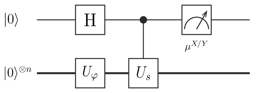
Figure 2: The Hadamard-test circuit $\mathcal{C}_{s}$. The qubit on the top is the ancilla qubit. The unitary operator $U_{\varphi}$ prepares the state $|{\varphi}\rangle$, i.e. $U_{\varphi}|{0}\rangle^{\otimes n}=|{\varphi}\rangle$. When the ancilla qubit is measured in the $X$ (or $Y$) basis, the measurement outcome is an eigenvalue of the Pauli operator $X$ (or $Y$), i.e. $\mu^{X}=\pm 1$ (or $\mu^{Y}=\pm 1$).

Given the LCU expression $A=\sum_{s}q_{s}U_{s}$, we can compute $\langle{\varphi}|A|{\varphi}\rangle$ using the Monte Carlo method and the one-ancilla Hadamard-test circuit shown in Fig. 2. In the Monte Carlo calculation, we sample the unitary operator $U_{s}$ with a probability of $|q_{s}|/C_{A}$ in the spirit of importance sampling. The corresponding algorithm is given in Algorithm 2.

1:Input $|{\varphi}\rangle$, $\{(q_{s},U_{s})\}$ and $M$.

2:$C_{A}\leftarrow\sum_{s}|q_{s}|$

3:$\hat{A}\leftarrow 0$

4:for $l=1$ to $M$ do

5:     Choose $s$ with a probability of $|q_{s}|/C_{A}$.

6:     Implement the circuit $\mathcal{C}_{s}$ for one shot, measure the ancilla qubit in the $X$ basis and record the measurement outcome $\mu^{X}$.

7:     Implement the circuit $\mathcal{C}_{s}$ for one shot, measure the ancilla qubit in the $Y$ basis and record the measurement outcome $\mu^{Y}$.

8:     $\hat{A}\leftarrow\hat{A}+e^{i\arg(q_{s})}(\mu^{X}+i\mu^{Y})$

9:Output $\hat{A}\leftarrow\frac{C_{A}}{M}\hat{A}$.

Algorithm 2 Monte Carlo evaluation of an LCU expression of $A$.

Lemma 8.

According to Algorithm 2, the estimator $\hat{A}$ is unbiased, and the variance upper bound in Eq. (6) is true.

Proof.

First, we rewrite the LCU expression as

$$A=C_{A}\sum_{s}\frac{|q_{s}|}{C_{A}}e^{i\arg(q_{s})}U_{s}.$$ (75)

Then,

$$\langle{\varphi}|A|{\varphi}\rangle=C_{A}\sum_{s}\frac{|q_{s}|}{C_{A}}e^{i\arg(q_{s})}\langle{\varphi}|U_{s}|{\varphi}\rangle.$$ (76)

Each unitary operator $U_{s}$ has a corresponding Hadamard-test circuit denoted by $\mathcal{C}_{s}$, which is shown in Fig. 2. When the ancilla qubit is measured in the $W=X,Y$ basis, the measurement has a random outcome $\mu^{W}=\pm 1$. Let $P^{W}_{\mu^{W}}$ be the probability of the measurement outcome $\mu^{W}$ in $\mathcal{C}_{s}$. According to Ref. Ekert et al. (2002), we have

$$\langle{\varphi}|U_{s}|{\varphi}\rangle=\sum_{\mu^{X}=\pm 1}P^{X}_{\mu^{X}}\mu^{X}+i\sum_{\mu^{Y}=\pm 1}P^{Y}_{\mu^{Y}}\mu^{Y}.$$ (77)

The probability of $(s,\mu^{X},\mu^{X})$ is $(|q_{s}|/C_{A})P^{X}_{\mu^{X}}P^{Y}_{\mu^{Y}}$. Using Eqs. (76) and (77), we have

$$\langle{\varphi}|A|{\varphi}\rangle=C_{A}\sum_{s,\mu^{X},\mu^{Y}}\frac{|q_{s}|}{C_{A}}P^{X}_{\mu^{X}}P^{Y}_{\mu^{Y}}e^{i\arg(q_{s})}(\mu^{X}+i\mu^{Y}).$$ (78)

The corresponding Monte Carlo algorithm is given in Algorithm 2.

The estimator $\hat{A}$ is unbiased. According to Eq. (78), the expected value of $C_{A}e^{i\arg(q_{s})}(\mu^{X}+i\mu^{Y})$ is $\langle{\varphi}|A|{\varphi}\rangle$. Therefore, the expected value of $\hat{A}$ is also $\langle{\varphi}|A|{\varphi}\rangle$. Notice that $\hat{A}$ is the average of $C_{A}e^{i\arg(q_{s})}(\mu^{X}+i\mu^{Y})$ over $M$ samples.

The variance of $\hat{A}$ is

$$\mathrm{Var}(\hat{A}) = \frac{1}{M}\left[\sum_{s,\mu^{X},\mu^{Y}}\frac{|q_{s}|}{C_{A}}P^{X}_{\mu^{X}}P^{Y}_{\mu^{Y}}\right.$$ (79)

$$\left.\times\left|C_{A}e^{i\arg(q_{s})}(\mu^{X}+i\mu^{Y})\right|^{2}-\left|\langle{\varphi}|A|{\varphi}\rangle\right|^{2}\right]$$

$$\leqslant \frac{2C_{A}^{2}}{M}.$$

∎

D.2.2 Cost upper bound

Substituting Eq. (66) into Eq. (5), we can obtain the eventual LCU expression of $f_{k}$. Substituting LCU expressions of $f_{k}$ and $f_{q}$ as well as the expression of $H$ into $A=f_{k}^{\dagger}Hf_{q},f_{k}^{\dagger}f_{q}$, we can obtain the LCU expression of $A$. It is straightforward to work out $C_{A}=h_{tot}c_{k}c_{q},c_{k}c_{q}$, respectively, where

$$c_{k}=\frac{1}{2^{\frac{k-1}{2}}\tau^{k-1}}\int_{-\infty}^{+\infty}dt\left|H_{k-1}\left(\frac{t}{\sqrt{2}\tau}\right)\right|g_{\tau}(t)[c(t/N)]^{N}.$$ (80)

Here, we have replaced $\left[\sum_{r}\left|v_{r}\left(\frac{t}{N}\right)\right|\right]^{N}$ with $[c(t/N)]^{N}$ in Eq. (8).

To work out the cost of $A$, we have used that the cost factor is additive and multiplicative. Suppose LCU expressions of $A_{1}$ and $A_{2}$ are $A_{1}=q_{1}U_{1}+q_{1}^{\prime}U_{1}^{\prime}$ and $A_{2}=q_{2}U_{2}+q_{2}^{\prime}U_{2}^{\prime}$, respectively. The cost factors of $A_{1}$ and $A_{2}$ are $C_{1}=|q_{1}|+|q_{1}^{\prime}|$ and $C_{2}=|q_{2}|+|q_{2}^{\prime}|$, respectively. Substituting LCU expressions of $A_{1}$ and $A_{2}$ into $A=A_{1}+A_{2}$, the expression of $A$ reads $A=q_{1}U_{1}+q_{1}^{\prime}U_{1}^{\prime}+q_{2}U_{2}+q_{2}^{\prime}U_{2}^{\prime}$. Then, the cost factor of $A$ is $C_{A}=|q_{1}|+|q_{1}^{\prime}|+|q_{2}|+|q_{2}^{\prime}|=C_{1}+C_{2}$. Substituting LCU expressions of $A_{1}$ and $A_{2}$ into $A^{\prime}=A_{1}A_{2}$, the expression of $A^{\prime}$ reads $A^{\prime}=(q_{1}U_{1}+q_{1}^{\prime}U_{1}^{\prime})(q_{2}U_{2}+q_{2}^{\prime}U_{2}^{\prime})=q_{1}q_{2}U_{1}U_{2}+q_{1}q_{2}^{\prime}U_{1}U_{2}^{\prime}+q_{1}^{\prime}q_{2}U_{1}^{\prime}U_{2}+q_{1}^{\prime}q_{2}^{\prime}U_{1}^{\prime}U_{2}^{\prime}$. Then, the cost factor of $A^{\prime}$ is $C_{A}^{\prime}=|q_{1}q_{2}|+|q_{1}q_{2}^{\prime}|+|q_{1}^{\prime}q_{2}|+|q_{1}^{\prime}q_{2}^{\prime}|=C_{1}C_{2}$.

The upper bound of $c_{k}$ is

$$c_{k}\leqslant c_{k}^{ub}=\frac{1}{2^{\frac{k-1}{2}}\tau^{k-1}}\int_{-\infty}^{+\infty}dt\left|H_{k-1}\left(\frac{t}{\sqrt{2}\tau}\right)\right|g_{\tau}(t)e^{\chi\frac{t^{2}}{\tau^{2}}},$$ (81)

where $\chi=\frac{eh_{tot}^{2}\tau^{2}}{2N}$. Here, we have used Lemma 7. Taking $\chi=\frac{1}{8}$ (i.e. $N=4eh_{tot}^{2}\tau^{2}$), we numerically evaluate the upper bound $c_{k}^{ub}$ and plot it in Fig. 3. We can find that

$$c_{k}^{ub}\leqslant 2\left(\frac{k-1}{e\tau^{2}}\right)^{\frac{k-1}{2}}.$$ (82)

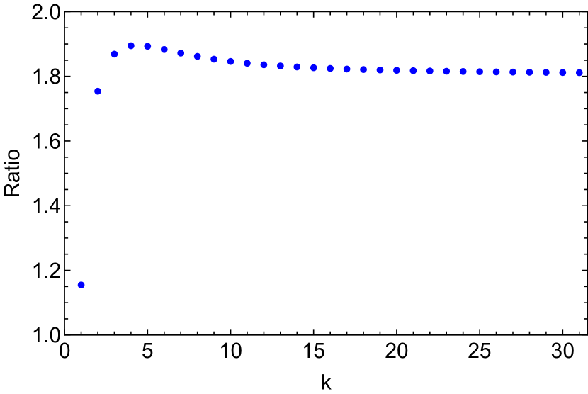
Figure 3: The ratio between cost upper bound and norm upper bound, $c_{k}^{ub}/[(k-1)/(e\tau^{2})]^{(k-1)/2}$.

D.3 Pseudocode

Given the LCU expression of $A$, we can compute $\langle{\varphi}|A|{\varphi}\rangle$ according to Algorithm 2. We would like to repeat how we compose the LCU expression of $A$: Substituting Eq. (66) into Eq. (5), we can obtain the eventual LCU expression of $f_{k}$; Substituting LCU expressions of $f_{k}$ and $f_{q}$ as well as the expression of $H$ into $A=f_{k}^{\dagger}Hf_{q}$ and $A=f_{k}^{\dagger}f_{q}$ (corresponding to $\mathbf{H}_{k,q}$ and $\mathbf{S}_{k,q}$, respectively), we can obtain the LCU expression of $A$. Algorithm 2 does not involve details of the LCU expression. In this section, we give pseudocodes involving details.

We remark that matrix entries of the rescaled basis $f^{\prime}_{k}=f_{k}/c_{k}$ are $\mathbf{H}^{\prime}_{k,q}=\mathbf{H}_{k,q}/(c_{k}c_{q})$ and $\mathbf{S}^{\prime}_{k,q}=\mathbf{S}_{k,q}/(c_{k}c_{q})$, where $\mathbf{H}_{k,q}$ and $\mathbf{S}_{k,q}$ are computed by the pseudocodes.

In pseudocodes, we use notations $\mathbf{h}=(h_{1},h_{2},\ldots)$ and $\bm{\sigma}=(\sigma_{1},\sigma_{2},\ldots)$ to represent the Hamiltonian $H=\sum_{j}h_{j}\sigma_{j}$. We define probability density functions

$$p_{\tau,k}(t)=\frac{1}{c_{k}2^{\frac{k-1}{2}}\tau^{k-1}}\left|H_{k-1}\left(\frac{t}{\sqrt{2}\tau}\right)\right|g_{\tau}(t)[c(t/N)]^{N},$$ (83)

and probabilities

$$P_{\mathrm{L}}(\Delta t) = \frac{\sqrt{1+h_{tot}^{2}\Delta t^{2}}}{c(\Delta t)},$$ (84)

$$P_{\mathrm{T}}(\Delta t) = \frac{e^{h_{tot}|\Delta t|}-(1+h_{tot}|\Delta t|)}{c(\Delta t)}.$$ (85)

We use $\text{P{\scriptsize OISSON}}(\lambda)$ to denote a subroutine that returns $k$ with a probability of $\lambda^{k}e^{-\lambda}/k!$.

1:Input $|{\varphi}\rangle$, $(\mathbf{h},\bm{\sigma})$, $E_{0}$, $\tau$, $N$ and $M$.

2:$h_{tot}\leftarrow\sum_{j}|h_{j}|$

3:Compute $c_{k}$ and $c_{q}$.

4:$\hat{\mathbf{H}}_{k,q}\leftarrow 0$

5:for $l=1$ to $M$ do

6:     Choose $j$ with a probability of $|h_{j}|/h_{tot}$.

7:     $(\bar{v}_{k},\bar{V}_{k})$ $\leftarrow$ BasisGen($\mathbf{h}$,$\bm{\sigma}$,$E_{0}$,$\tau$,$N$,$k$)

8:     $(\bar{v}_{q},\bar{V}_{q})$ $\leftarrow$ BasisGen($\mathbf{h}$,$\bm{\sigma}$,$E_{0}$,$\tau$,$N$,$q$)

9:     Implement the circuit $\mathcal{C}_{s}$ with $U_{s}=\bar{V}_{k}^{\dagger}\sigma_{j}\bar{V}_{q}$ for one shot, measure the ancilla qubit in the $X$ basis and record the measurement outcome $\mu^{X}$.

10:     Implement the circuit $\mathcal{C}_{s}$ with $U_{s}=\bar{V}_{k}^{\dagger}\sigma_{j}\bar{V}_{q}$ for one shot, measure the ancilla qubit in the $Y$ basis and record the measurement outcome $\mu^{Y}$.

11:     $\hat{\mathbf{H}}_{k,q}\leftarrow\hat{\mathbf{H}}_{k,q}+e^{i\arg(\bar{v}_{k}^{*}h_{j}\bar{v}_{q})}(\mu^{X}+i\mu^{Y})$

12:Output $\hat{\mathbf{H}}_{k,q}\leftarrow\frac{h_{tot}c_{k}c_{q}}{M}\hat{\mathbf{H}}_{k,q}$.

Algorithm 3 Measurement of matrix entry $\mathbf{H}_{k,q}$.

1:Input $|{\varphi}\rangle$, $(\mathbf{h},\bm{\sigma})$, $E_{0}$, $\tau$, $N$ and $M$.

2:Compute $c_{k}$ and $c_{q}$.

3:$\hat{\mathbf{S}}_{k,q}\leftarrow 0$

4:for $l=1$ to $M$ do

5:     $(\bar{v}_{k},\bar{V}_{k})$ $\leftarrow$ BasisGen($\mathbf{h}$,$\bm{\sigma}$,$E_{0}$,$\tau$,$N$,$k$)

6:     $(\bar{v}_{q},\bar{V}_{q})$ $\leftarrow$ BasisGen($\mathbf{h}$,$\bm{\sigma}$,$E_{0}$,$\tau$,$N$,$q$)

7:     Implement the circuit $\mathcal{C}_{s}$ with $U_{s}=\bar{V}_{k}^{\dagger}\bar{V}_{q}$ for one shot, measure the ancilla qubit in the $X$ basis and record the measurement outcome $\mu^{X}$.

8:     Implement the circuit $\mathcal{C}_{s}$ with $U_{s}=\bar{V}_{k}^{\dagger}\bar{V}_{q}$ for one shot, measure the ancilla qubit in the $Y$ basis and record the measurement outcome $\mu^{Y}$.

9:     $\hat{\mathbf{S}}_{k,q}\leftarrow\hat{\mathbf{S}}_{k,q}+e^{i\arg(\bar{v}_{k}^{*}\bar{v}_{q})}(\mu^{X}+i\mu^{Y})$

10:Output $\hat{\mathbf{S}}_{k,q}\leftarrow\frac{c_{k}c_{q}}{M}\hat{\mathbf{S}}_{k,q}$.

Algorithm 4 Measurement of matrix entry $\mathbf{S}_{k,q}$.

1:function BasisGen($\mathbf{h}$,$\bm{\sigma}$,$E_{0}$,$\tau$,$N$,$k$)

2:     Generate random time $t$ according to the distribution $p_{\tau,k}(t)$.

3:     $(\bar{v},\bar{V})$ $\leftarrow$ RTE($\mathbf{h}$,$\bm{\sigma}$,$N$,$t$)

4:     $\bar{v}\leftarrow\bar{v}\times\frac{i^{k-1}}{2^{\frac{k-1}{2}}\tau^{k-1}}H_{k-1}\left(\frac{t}{\sqrt{2}\tau}\right)g_{\tau}(t)e^{iE_{0}t}$

5:     Output $(\bar{v},\bar{V})$.

Algorithm 5 Basis generator $f_{k}$.

1:function RTE($\mathbf{h}$,$\bm{\sigma}$,$N$,$t$)

2:     $\bar{v}\leftarrow 1$

3:     $\bar{V}\leftarrow\openone$

4:     for $i=1$ to $N$ do

5:         $(v,V)$ $\leftarrow$ LORF($\mathbf{h}$,$\bm{\sigma}$,$t/N$)

6:         $\bar{v}\leftarrow\bar{v}\times v$

7:         $\bar{V}\leftarrow\bar{V}\times V$      

8:     Output $(\bar{v},\bar{V})$.

Algorithm 6 Real-time evolution.

1:function LORF($\mathbf{h}$,$\bm{\sigma}$,$\Delta t$)

2:     Choose $\mathrm{O}$ from $\mathrm{L}$ and $\mathrm{T}$ with probabilities of $P_{\mathrm{L}}(\Delta t)$ and $P_{\mathrm{T}}(\Delta t)$, respectively.

3:     if $\mathrm{O}=\mathrm{L}$ then

4:         Choose $j$ with a probability of $|h_{j}|/h_{tot}$.

5:         $v\leftarrow\beta_{j}(\Delta t)$

6:         $V\leftarrow e^{-i\mathrm{sgn}(h_{j})\phi(\Delta t)\sigma_{j}}$

7:     else if $\mathrm{O}=\mathrm{T}$ then

8:         while $k<2$ do

9:              $k\leftarrow\textsc{Poisson}(h_{tot}|\Delta t|)$          

10:         $v\leftarrow 1/k!$

11:         $V\leftarrow\openone$

12:         for $a=1$ to $k$ do

13:              Choose $j$ with a probability of $|h_{j}|/h_{tot}$.

14:              $v\leftarrow v\times(-ih_{j}\Delta t)$

15:              $V\leftarrow V\times\sigma_{j}$               

16:     Output $(v,V)$.

Algorithm 7 Leading-order-rotation formula.

Appendix E Details in numerical calculation

In this section, first, we describe models and reference states taken in the benchmarking, and then we give details.

E.1 Models and reference states

Two models are used in the benchmarking: the anti-ferromagnetic Heisenberg model

$$H=J\sum_{\langle i,j\rangle}(\sigma^{X}_{i}\sigma^{X}_{j}+\sigma^{Y}_{i}\sigma^{Y}_{j}+\sigma^{Z}_{i}\sigma^{Z}_{j}),$$ (86)

where $\sigma^{X}_{i}$, $\sigma^{Y}_{i}$ and $\sigma^{Z}_{i}$ are Pauli operators of the $i$th qubit; and the Hubbard model

$$H = -J\sum_{\langle i,j\rangle}\sum_{\sigma=\uparrow,\downarrow}(a_{i,\sigma}^{\dagger}a_{j,\sigma}+a_{j,\sigma}^{\dagger}a_{i,\sigma})$$ (87)

$$+U\sum_{i}\left(a_{i,\uparrow}^{\dagger}a_{i,\uparrow}-\frac{\openone}{2}\right)\left(a_{i,\downarrow}^{\dagger}a_{i,\downarrow}-\frac{\openone}{2}\right),$$

where $a_{i,\sigma}$ is the annihilation operator of the $i$th orbital and spin $\sigma$. For the Heisenberg model, we take the spin number as ten, and for the Hubbard model, we take the orbital number as five. Then both models can be encoded into ten qubits. For the Hubbard model, we take $U=J$. Without loss of generality, we normalise the Hamiltonian for simplicity: We take $J$ such that $\|H\|_{2}=1$, i.e. eigenvalues of $H$ are in the interval $[-1,1]$.

For each model, we consider three types of lattices: chain, ladder and randomly generated graphs, see Fig. 4. We generate a random graph in the following way: i) For a vertex $v$, randomly choose a vertex $u\neq v$ and add the edge $(v,u)$; ii) Repeat step-i two times for the vertex $v$; iii) Implement steps i and ii for each vertex $v$. On a graph generated in this way, each vertex is connected to four vertices on average. Notice that some pairs of vertices are connected by multiple edges, and then the interaction between vertices in the pair is amplified by the number of edges.

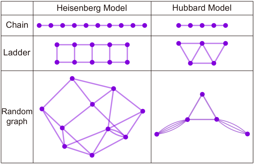
Figure 4: Lattices of the Heisenberg model and Hubbard model. One of the randomly generated graphs for each model is illustrated in the figure as an example.

It is non-trivial to choose and prepare a good reference state that has a sufficiently large overlap with the true ground state. Finding the ground-state energy of a local Hamiltonian is QMA-hard Kitaev et al. (2002); Kempe et al. (2006). If one can prepare a good reference state, then quantum computing is capable of solving the ground-state energy using quantum phase estimation Gharibian et al. . So far, there does not exist a universal method for reference state preparation; see Ref. Lee et al. for relevant discussions. Despite this, there are some practical ways of choosing and preparing the reference state. For fermion systems, we can take the mean-field approximate solution, i.e. a Hartree-Fock state, as the reference state. For general systems, one may try adiabatic state preparation, etc. We stress that preparing good reference states is beyond the scope of this work. Here, we choose two reference states which are likely to overlap with true ground states as examples. For the Heisenberg model, we take the pairwise singlet state

$$|{\varphi}\rangle = |{\Phi}\rangle_{1,2}\otimes|{\Phi}\rangle_{3,4}\otimes\cdots,$$ (88)

where

$$|{\Phi}\rangle_{i,j}=\frac{1}{\sqrt{2}}\left(|{0}\rangle_{i}\otimes|{1}\rangle_{j}-|{1}\rangle_{i}\otimes|{0}\rangle_{j}\right)$$ (89)

is the singlet state of spins $i$ and $j$. For the Hubbard model, we take a Hartree-Fock state as the reference state: We compute the ground state of the one-particle Hamiltonian (which is equivalent to taking $U=0$) and take the ground state of the one-particle Hamiltonian (a Slater determinant) as the reference state.

E.2 Instances

We test the algorithms listed in Table 1 with many instances. Each instance is a triple $(model,lattice,d)$, in which $model$ takes one of the two models (Heisenberg model and Hubbard model), $lattice$ takes a chain, ladder or random graph, and $d$ is the dimension of the subspace. For example, Fig. 5 shows the result of instance $(\mathrm{Heisenberg},\mathrm{chain},d=5)$.

Figure 5: Comparison between quantum KSD algorithms listed in Table 1. Here, we take the instance $(\mathrm{Heisenberg},\mathrm{chain},d=5)$ as an example. $\epsilon_{K}$ is the subspace error of the P algorithm. The grey area illustrates the range of $\gamma$ when we take $E_{0}\in[E_{g}-0.1,E_{g}+0.1]$ in the GP algorithm. Notice that $\|H\|_{2}=1$. The blue curve represents the result of the GP algorithm with $E_{0}=E_{g}$.

Instances for computing empirical distributions in Fig. 1 consist of six groups: the Heisenberg model on the chain, ladder and random graphs, and the Hubbard model on the chain, ladder and random graphs. For chain and ladder, we evaluate each subspace dimension $d=2,3,\ldots,30$; For a random graph, we only evaluate one subspace dimension randomly taken in the interval. Some instances are discarded. To avoid any potential issue caused by the precision of floating-point numbers, we discard instances that the subspace error $\epsilon_{K}$ of the P algorithm is lower than $10^{-9}$ due to a large $d$. We also discard instances that $\epsilon_{K}$ of the P algorithm is higher than $10^{-2}$ due to a small $d$, because the dimension may be too small to achieve an interesting accuracy in this case. For randomly generated graphs, the two reference states may have a small overlap with the true ground state. Because a good reference state is necessary for all quantum KSD algorithms, we discard graphs with $p_{g}<10^{-3}$. Eventually, we have eight instances of the Heisenberg chain, seven instances of the Heisenberg Ladder, twenty-two instances of the Hubbard chain and twenty instances of the Hubbard ladder. For each model, we generate a hundred random-graph instances. The total number of instances is $257$.

E.3 Parameters

Abbr.	$E_{0}$	$\tau$	$\Delta t$	$\Delta E$	$C_{\mathbf{H}}$	$C_{\mathbf{S}}$
P	$E_{g}+1$	N/A	N/A	N/A	$1$	$1$
CP	$0$	N/A	N/A	N/A	$1$	$1$
GP	$[E_{g}-0.1,E_{g}+0.1]$	Solving Eq. (91)	N/A	N/A	$h_{tot}\geqslant 1$	$1$
IP	$E_{g}-1$	N/A	N/A	N/A	$1$	$1$
ITE	$E_{g}$	Solving Eq. (92)	N/A	N/A	$1$	$1$
RTE	$E_{g}$	N/A	Minimising $\epsilon_{K}$	N/A	$1$	$1$
F	$E_{g}$	Solving Eq. (91)	$2\tau/(L-1)$	Minimising $\epsilon_{K}$	$1$	$1$

Table 2: Parameters taken in the numerical calculation.

In this section, we give parameters taken in each algorithm listed in Table 1, namely, $E_{0}$, $\tau$, $\Delta t$, $\Delta E$, $C_{\mathbf{H}}$ and $C_{\mathbf{S}}$. We summarise these parameters in Table 2.

For $E_{0}$, we expect that taking $E_{0}$ close to $E_{g}$ is optimal for our GP algorithm. As the exact value of $E_{g}$ is unknown, we assume that we have a preliminary estimation of the ground-state energy with uncertainty as large as $10\%$ of the entire spectrum, i.e. we take $E_{0}\in[E_{g}-0.1,E_{g}+0.1]$. For other algorithms, we take $E_{0}$ by assuming that the exact value of $E_{g}$ is known. In the P algorithm, we take $E_{0}=E_{g}+1$, such that the ground state is the eigenstate of $H-E_{0}$ with the largest absolute eigenvalue and $\|H-E_{0}\|_{2}=1$. Similarly, in the IP algorithm, we take $E_{0}=E_{g}-1$, such that the ground state is the eigenstate of $(H-E_{0})^{-1}$ with the largest absolute eigenvalue and $\|(H-E_{0})^{-1}\|_{2}=1$. In the ITE algorithm, $E_{0}$ causes a constant factor $e^{\tau(k-1)E_{0}}$ in each operator $f_{k}$, i.e. determines the spectral norm of $f_{k}$. Because the variance is related to the norm, a large $E_{0}$ is problematic. Therefore, in the ITE algorithm, we take $E_{0}=E_{g}$, such that $\|f_{k}\|=1$ for all $k$. In the F algorithm, we expect that $E_{0}=E_{g}$ is optimal because $f_{1}$ is an energy filter centred at the ground-state energy in this case. Therefore, we take $E_{0}=E_{g}$ in the F algorithm. The RTE algorithm is closely related to the F algorithm. Therefore, we also take $E_{0}=E_{g}$ in the RTE algorithm.

We remark that in the GP algorithm, we take random $E_{0}$ uniformly distributed in the interval $[E_{g}-0.1,E_{g}+0.1]$ to generate data in Fig. 1, and we take $E_{0}=-E_{g}+i\delta E$, where $i=-50,-9,\ldots,-1,0,1,\ldots,9,50$ and $\delta E=0.002$, to generate data in Fig. 5. We remark that we have normalised the Hamiltonian such that $\|H\|_{2}=1$.

For $\Delta t$ in the F algorithm, we take $\Delta t=2\tau/(L-1)$. For simplicity, we take the limit $L\rightarrow+\infty$, i.e.

$$f_{k} = \frac{1}{2\tau}\int_{-\tau}^{\tau}dte^{-i\left[H-E_{0}-\Delta E\left(k-1\right)\right]t}$$ (90)

$$= \frac{\sin\left[H-E_{0}-\Delta E\left(k-1\right)\right]\tau}{\left[H-E_{0}-\Delta E\left(k-1\right)\right]\tau}.$$

Notice that this $f_{k}$ is an energy filter centred at $E_{0}+\Delta E\left(k-1\right)$, and the filter is narrower when $\tau$ is larger.

Now, we have three algorithms that have the parameter $\tau$: GP, ITE and F. Similar to the F algorithm, $f_{1}$ in the GP algorithm is an energy filter centred at $E_{0}$. For these two algorithms, if $E_{0}=E_{g}$, $f_{1}|{\varphi}\rangle$ converges to the true ground state in the limit $\tau\rightarrow+\infty$. It is also similar in the ITE algorithm, in which $f_{d}$ is a projector onto the ground state, and $f_{d}|{\varphi}\rangle$ converges to the true ground state in the limit $\tau\rightarrow+\infty$. Realising a large $\tau$ is at a certain cost, specifically, the circuit depth increases with $\tau$ Berry et al. (2007); Motta et al. (2019). Therefore, it is reasonable to take a finite $\tau$. Next, we give the protocol for determining the value of $\tau$ in each algorithm.

Without getting into details about realising the filters and projectors, we choose $\tau$ under the assumption that if filters and projectors have the same power in computing the ground-state energy, they probably require similar circuit depths. In GP and F algorithms, if $E_{0}=E_{g}$, the energy error achieved by filters reads $\mathbf{H}_{1,1}/\mathbf{S}_{1,1}-E_{g}$; and in the ITE algorithm, the energy error achieved by the projector reads $\mathbf{H}_{d,d}/\mathbf{S}_{d,d}-E_{g}$. We take $\tau$ such that errors achieved by filters and projectors take the same value $\epsilon_{B}$. Specifically, for the GP and F algorithms, we determine the value of $\tau$ by solving the equation (taking $E_{0}=E_{g}$)

$$\frac{\mathbf{H}_{1,1}(\tau)}{\mathbf{S}_{1,1}(\tau)}-E_{g}=\epsilon_{B};$$ (91)

and for the ITE algorithm, we determine the value of $\tau$ by solving the equation

$$\frac{\mathbf{H}_{d,d}(\tau)}{\mathbf{S}_{d,d}(\tau)}-E_{g}=\epsilon_{B}.$$ (92)

To choose the value of $\epsilon_{B}$, we take the P algorithm as the standard, in which $f_{d}$ is a projector onto the ground state, i.e. $f_{d}|{\varphi}\rangle$ converges to the true ground state in the limit $d\rightarrow+\infty$. Overall, we determine the value of $\tau$ in the following way: Given an instance $(model,lattice,d)$, i) first, compute the energy error achieved by the projector in the P algorithm, take $\epsilon_{B}=\mathbf{H}_{d,d}/\mathbf{S}_{d,d}-E_{g}$; then, ii) solve equations of $\tau$. In this way, filters and projectors in P, GP, ITE and F algorithms have the same power.

For $\Delta t$ in the RTE algorithm and $\Delta E$ in the F algorithm, there are works on how to choose them in the literature Klymko et al. (2022); Shen et al. ; Cortes and Gray (2022). In this work, we simply determine their values by a grid search. For the RTE algorithm, we take $\Delta t=i\delta t$, where $i=1,2,\ldots,100$ and $\delta t=\frac{2\pi}{100}$; we compute the subspace error $\epsilon_{K}$ for all $\Delta t$; and we choose $\Delta t$ of the minimum $\epsilon_{K}$. For the F algorithm, we take $\Delta E=i\delta E$, where $i=1,2,\ldots,100$ and $\delta E=\frac{2}{100d}$ (In this way, when we take the largest $\Delta E$, filters span the entire spectrum); we compute the subspace error $\epsilon_{K}$ for all $\Delta E$; and we choose $\Delta E$ of the minimum $\epsilon_{K}$.

For $C_{\mathbf{H}}$ and $C_{\mathbf{S}}$, we take $C_{\mathbf{H}}=h_{tot}$ and $C_{\mathbf{S}}=1$ in our GP algorithm following the analysis in Appendix D. For other algorithms, we take these two parameters in the following way. For P, IP, ITE and RTE algorithms, we take $C_{\mathbf{H}}$ and $C_{\mathbf{S}}$ according to spectral norms (the lower bound of cost) without getting into details about measuring matrix entries. In these four algorithms, $\|f_{k}^{\dagger}Hf_{q}\|_{2}=\|f_{k}^{\dagger}f_{q}\|_{2}=1$ for all $k$ and $q$, therefore, we take $C_{\mathbf{H}}=C_{\mathbf{S}}=1$. In the CP algorithm, we take $C_{\mathbf{H}}$ and $C_{\mathbf{S}}$ in a similar way. Because $\|H/h_{tot}\|_{2}\leqslant 1$, the spectrum of $H/h_{tot}$ is in the interval $[-1,1]$. In this interval, the Chebyshev polynomial of the first kind takes values in the interval $[-1,1]$. Therefore, $\|T_{k}(H/h_{tot})\|_{2}\leqslant 1$, and consequently $\|f_{k}^{\dagger}Hf_{q}\|_{2},\|f_{k}^{\dagger}f_{q}\|_{2}\leqslant 1$. These norms depend on the spectrum of $H$. For simplicity, we take the upper bound of norms, i.e. $C_{\mathbf{H}}=C_{\mathbf{S}}=1$, in the CP algorithm. In the F algorithm, each $f_{k}$ is a linear combination of $e^{-iHt}$ operators, i.e. $f_{k}$ is expressed in the LCU form, and the cost factor of the LCU expression is one. Therefore, we take $C_{\mathbf{H}}=C_{\mathbf{S}}=1$ in the F algorithm, assuming that $H$ is expressed in the LCU form with a cost factor of one (Notice that one is the lower bound).

Appendix F Composing Chebyshev polynomials

F.1 Chebyshev-polynomial projector

In this section, we explain how to use Chebyshev polynomials as projectors onto the ground state.

The $n$th Chebyshev polynomial of the first kind is

$$T_{n}(z)=\left\{\begin{array}[]{cc}\cos(n\arccos z),&\text{if }|z|\leqslant 1,\\ \mathrm{sgn}(z)^{n}\cosh(n\,\mathrm{arccosh}|z|),&\text{if }|z|>1.\end{array}\right.$$ (95)

Chebyshev polynomials have the following properties: i) When $|z|\leqslant 1$, $|T_{n}(z)|\leqslant 1$; and ii) when $|z|>1$, $|T_{n}(z)|>(|z|^{n}+|z|^{-n})/2$ increases exponentially with $n$.

Let’s consider the spectral decomposition of the Hamiltonian, $H=\sum_{m=1}^{d_{\mathcal{H}}}E_{m}|\psi_{m}\rangle\langle\psi_{m}|$. Here, $d_{\mathcal{H}}$ is the dimension of the Hilbert space, $E_{m}$ are eigenenergies of the Hamiltonian, and $|{\psi_{m}}\rangle$ are eigenstates. We suppose that eigenenergies are sorted in ascending order, i.e. $E_{i}\leqslant E_{j}$ if $i<j$. Then, $E_{1}=E_{g}$ is the ground-state energy (accordingly, $|{\psi_{1}}\rangle=|{\psi_{g}}\rangle$ is the ground state) and $E_{2}$ is the energy of the first excited state. The energy gap between the ground state and the first excited state is $\Delta=E_{2}-E_{1}$.

To compose a projector, we take

$$Z=1-\frac{H-E_{2}}{\|H\|_{2}}.$$ (96)

Notice that $Z$ and $H$ have the same eigenstates. The spectral decomposition of $Z$ is $Z=\sum_{m=1}^{d_{\mathcal{H}}}z_{m}|\psi_{m}\rangle\langle\psi_{m}|$, where

$$z_{m}=1-\frac{E_{m}-E_{2}}{\|H\|_{2}}.$$ (97)

Then, the ground state corresponds to $z_{1}=1+\frac{\Delta}{\|H\|_{2}}>1$ (suppose the gap is finite), and the first excited state corresponds to $z_{2}=1$. Because $|E_{m}-E_{2}|\leqslant 2\|H\|_{2}$, $z_{m}\geqslant-1$ for all $m$. Therefore, except the ground state, $x_{m}$ of all excited states (i.e. $m\geqslant 2$) is in the interval $[-1,1]$.

The projector reads

$$\frac{T_{n}(Z)}{T_{n}(z_{1})} = \sum_{m=1}^{d_{\mathcal{H}}}\frac{T_{n}(z_{m})}{T_{n}(z_{1})}|\psi_{m}\rangle\langle\psi_{m}|$$ (98)

$$= |\psi_{g}\rangle\langle\psi_{g}|+\Omega,$$

where

$$\Omega = \sum_{m=2}^{d_{\mathcal{H}}}\frac{T_{n}(z_{m})}{T_{n}(z_{1})}|\psi_{m}\rangle\langle\psi_{m}|.$$ (99)

$\Omega$ and $H$ have the same eigenstates. Because $|T_{n}(z_{m})|\leqslant 1$ when $m\geqslant 2$,

$$\|\Omega\|_{2}\leqslant\frac{1}{T_{n}(z_{1})}.$$ (100)

The key in using Chebyshev polynomials as projectors is laying all excited states in the interval $z\in[-1,1]$ and leaving the ground state out of the interval. For the CP basis, all eigenstates are in the interval $z\in[-1,1]$. Therefore, $f_{k}$ operators of the CP basis are not projectors in general.

F.2 Expanding the projector as Hamiltonian powers

In this section, we expand the Chebyshev-polynomial projector as a linear combination of Hamiltonian powers $(H-E_{0})^{k-1}$. We focus on the case that $E_{0}=E_{g}$.

The explicit expression of $T_{n}(z)$ ($n>0$) is

$$T_{n}(z)=n\sum_{m=0}^{n}(-2)^{m}\frac{(n+m-1)!}{(n-m)!(2m)!}(1-z)^{m}.$$ (101)

Because

$$(1-Z)^{m}=\sum_{l=0}^{m}\frac{m!}{(m-l)!l!}\frac{(E_{0}-E_{2})^{m-l}(H-E_{0})^{l}}{\|H\|_{2}^{m}},$$ (102)

we have

$$T_{n}(Z)=\sum_{l=0}^{n}b_{l}\frac{(H-E_{0})^{l}}{\|H\|_{2}^{l}},$$ (103)

where

$$b_{l}=n\sum_{m=l}^{n}(-2)^{m}\frac{(n+m-1)!}{(n-m)!(2m)!}\frac{m!}{(m-l)!l!}\frac{(E_{0}-E_{2})^{m-l}}{\|H\|_{2}^{m-l}}.$$ (104)

Now, we give an upper bound of $|b_{l}|$. First, we consider $l=0$. In this case,

$$|b_{0}| \leqslant n\sum_{m=0}^{n}2^{m}\frac{(n+m-1)!}{(n-m)!(2m)!}\frac{|E_{0}-E_{2}|^{m}}{\|H\|_{2}^{m}}$$ (105)

$$= T_{n}(z_{1}).$$

Then, for an arbitrary $l$,

$$|b_{l}| \leqslant n^{l}T_{n}(z_{1}),$$ (106)

where the inequality

$$\frac{m!}{(m-l)!l!} \leqslant m^{l}\leqslant n^{l}$$ (107)

has been used.

Finally, taking $d=n+1$ and

$$a_{k}=\frac{c_{k}b_{k-1}}{T_{n}(z_{1})\|H\|_{2}^{k-1}},$$ (108)

we have

$$\sum_{k=1}^{d}a_{k}c_{k}^{-1}f_{k}=\frac{T_{n}(Z)}{T_{n}(z_{1})}e^{-\frac{1}{2}(H-E_{0})^{2}\tau^{2}},$$ (109)

where $f_{k}$ are operators defined in Eq. (4). Because of the upper bound

$$|a_{k}| \leqslant 2\left(\frac{k-1}{e\tau^{2}}\right)^{\frac{k-1}{2}}\left(\frac{n}{\|H\|_{2}}\right)^{k-1}$$ (110)

$$\leqslant 2\left(\frac{n^{3}}{e\|H\|_{2}^{2}\tau^{2}}\right)^{\frac{k-1}{2}},$$

the overhead factor is

$$\gamma \approx \left(\mathbf{a}^{\dagger}\mathbf{a}\right)^{2}\leqslant 4\sum_{k=1}^{d}\left(\frac{n^{3}}{e\|H\|_{2}^{2}\tau^{2}}\right)^{k-1}$$ (111)

$$\leqslant 4\frac{1}{1-n^{3}/(e\|H\|_{2}^{2}\tau^{2})}.$$

References

- Dagotto (1994) Elbio Dagotto, “Correlated electrons in high-temperature superconductors,” Reviews of Modern Physics 66, 763 (1994).
- Wall and Neuhauser (1995) Michael R Wall and Daniel Neuhauser, “Extraction, through filter-diagonalization, of general quantum eigenvalues or classical normal mode frequencies from a small number of residues or a short-time segment of a signal. i. theory and application to a quantum-dynamics model,” The Journal of chemical physics 102, 8011–8022 (1995).
- Caurier et al. (2005) Etienne Caurier, Gabriel Martínez-Pinedo, Fréderic Nowacki, Alfredo Poves, and AP Zuker, “The shell model as a unified view of nuclear structure,” Reviews of modern Physics 77, 427 (2005).
- Lanczos (1950) Cornelius Lanczos, “An iteration method for the solution of the eigenvalue problem of linear differential and integral operators,” Journal of research of the National Bureau of Standards 45, 255–282 (1950).
- Saad (2011) Yousef Saad, Numerical Methods for Large Eigenvalue Problems (Society for Industrial and Applied Mathematics, 2011).
- Björck (2015) Åke Björck, Numerical methods in matrix computations, Vol. 59 (Springer, 2015).
- Avella and Mancini (2013) Adolfo Avella and Ferdinando Mancini, Strongly Correlated Systems, Vol. 176 (Springer, 2013).
- Motta et al. (2019) Mario Motta, Chong Sun, Adrian T. K. Tan, Matthew J. O’Rourke, Erika Ye, Austin J. Minnich, Fernando G. S. L. Brandão, and Garnet Kin-Lic Chan, “Determining eigenstates and thermal states on a quantum computer using quantum imaginary time evolution,” Nature Physics 16, 205–210 (2019).
- Yeter-Aydeniz et al. (2020) Kübra Yeter-Aydeniz, Raphael C Pooser, and George Siopsis, “Practical quantum computation of chemical and nuclear energy levels using quantum imaginary time evolution and lanczos algorithms,” npj Quantum Information 6, 1–8 (2020).
- (10) Robert M. Parrish and Peter L. McMahon, “Quantum filter diagonalization: Quantum eigendecomposition without full quantum phase estimation,” arXiv:1909.08925 .
- Stair et al. (2020) Nicholas H. Stair, Renke Huang, and Francesco A. Evangelista, “A multireference quantum krylov algorithm for strongly correlated electrons,” Journal of Chemical Theory and Computation 16, 2236–2245 (2020).
- Bespalova and Kyriienko (2021) Tatiana A Bespalova and Oleksandr Kyriienko, “Hamiltonian operator approximation for energy measurement and ground-state preparation,” PRX Quantum 2, 030318 (2021).
- Cohn et al. (2021) Jeffrey Cohn, Mario Motta, and Robert M Parrish, “Quantum filter diagonalization with compressed double-factorized hamiltonians,” PRX Quantum 2, 040352 (2021).
- Klymko et al. (2022) Katherine Klymko, Carlos Mejuto-Zaera, Stephen J Cotton, Filip Wudarski, Miroslav Urbanek, Diptarka Hait, Martin Head-Gordon, K Birgitta Whaley, Jonathan Moussa, Nathan Wiebe, et al., “Real-time evolution for ultracompact hamiltonian eigenstates on quantum hardware,” PRX Quantum 3, 020323 (2022).
- Cortes and Gray (2022) Cristian L Cortes and Stephen K Gray, “Quantum krylov subspace algorithms for ground-and excited-state energy estimation,” Physical Review A 105, 022417 (2022).
- Epperly et al. (2022) Ethan N Epperly, Lin Lin, and Yuji Nakatsukasa, “A theory of quantum subspace diagonalization,” SIAM Journal on Matrix Analysis and Applications 43, 1263–1290 (2022).
- (17) Yizhi Shen, Katherine Klymko, James Sud, David B Williams-Young, Wibe A de Jong, and Norm M Tubman, “Real-time krylov theory for quantum computing algorithms,” arXiv:2208.01063 .
- Kyriienko (2020) Oleksandr Kyriienko, “Quantum inverse iteration algorithm for programmable quantum simulators,” npj Quantum Information 6, 1–8 (2020).
- Seki and Yunoki (2021) Kazuhiro Seki and Seiji Yunoki, “Quantum power method by a superposition of time-evolved states,” PRX Quantum 2, 010333 (2021).
- (20) William Kirby, Mario Motta, and Antonio Mezzacapo, “Exact and efficient lanczos method on a quantum computer,” arXiv:2208.00567 .
- Babbush et al. (2018) Ryan Babbush, Craig Gidney, Dominic W. Berry, Nathan Wiebe, Jarrod McClean, Alexandru Paler, Austin Fowler, and Hartmut Neven, “Encoding electronic spectra in quantum circuits with linear t complexity,” Phys. Rev. X 8, 041015 (2018).
- Lee et al. (2021) Joonho Lee, Dominic W. Berry, Craig Gidney, William J. Huggins, Jarrod R. McClean, Nathan Wiebe, and Ryan Babbush, “Even more efficient quantum computations of chemistry through tensor hypercontraction,” PRX Quantum 2, 030305 (2021).
- Peruzzo et al. (2014) Alberto Peruzzo, Jarrod McClean, Peter Shadbolt, Man-Hong Yung, Xiao-Qi Zhou, Peter J Love, Alán Aspuru-Guzik, and Jeremy L O’brien, “A variational eigenvalue solver on a photonic quantum processor,” Nature communications 5, 4213 (2014).
- McClean et al. (2018) Jarrod R McClean, Sergio Boixo, Vadim N Smelyanskiy, Ryan Babbush, and Hartmut Neven, “Barren plateaus in quantum neural network training landscapes,” Nature communications 9, 4812 (2018).
- Parlett (1998) Beresford N. Parlett, The Symmetric Eigenvalue Problem (Society for Industrial and Applied Mathematics, 1998).
- Householder (2013) Alston S. Householder, The Theory of Matrices in Numerical Analysis (Dover Publications, 2013).
- McClean et al. (2017) Jarrod R. McClean, Mollie E. Kimchi-Schwartz, Jonathan Carter, and Wibe A. de Jong, “Hybrid quantum-classical hierarchy for mitigation of decoherence and determination of excited states,” Phys. Rev. A 95, 042308 (2017).
- Parrish et al. (2019) Robert M Parrish, Edward G Hohenstein, Peter L McMahon, and Todd J Martínez, “Quantum computation of electronic transitions using a variational quantum eigensolver,” Physical review letters 122, 230401 (2019).
- Nakanishi et al. (2019) Ken M Nakanishi, Kosuke Mitarai, and Keisuke Fujii, “Subspace-search variational quantum eigensolver for excited states,” Physical Review Research 1, 033062 (2019).
- Huggins et al. (2020) William J Huggins, Joonho Lee, Unpil Baek, Bryan O’Gorman, and K Birgitta Whaley, “A non-orthogonal variational quantum eigensolver,” New Journal of Physics 22, 073009 (2020).
- (31) Nicholas H Stair, Cristian L Cortes, Robert M Parrish, Jeffrey Cohn, and Mario Motta, “A stochastic quantum krylov protocol with double factorized hamiltonians,” arXiv:2211.08274 .
- McClean et al. (2020) Jarrod R McClean, Zhang Jiang, Nicholas C Rubin, Ryan Babbush, and Hartmut Neven, “Decoding quantum errors with subspace expansions,” Nature communications 11, 636 (2020).
- Yoshioka et al. (2022) Nobuyuki Yoshioka, Hideaki Hakoshima, Yuichiro Matsuzaki, Yuuki Tokunaga, Yasunari Suzuki, and Suguru Endo, “Generalized quantum subspace expansion,” Phys. Rev. Lett. 129, 020502 (2022).
- Horn and Johnson (2012) Roger A. Horn and Charles R. Johnson, Matrix Analysis, 2nd ed. (Cambridge University Press, 2012).
- Huo and Li (2023) Mingxia Huo and Ying Li, “Error-resilient monte carlo quantum simulation of imaginary time,” Quantum 7, 916 (2023).
- (36) Pei Zeng, Jinzhao Sun, and Xiao Yuan, “Universal quantum algorithmic cooling on a quantum computer,” arXiv:2109.15304 .
- Childs and Wiebe (2012) Andrew M Childs and Nathan Wiebe, “Hamiltonian simulation using linear combinations of unitary operations,” Quantum Information & Computation 12, 901–924 (2012).
- Ekert et al. (2002) Artur K Ekert, Carolina Moura Alves, Daniel KL Oi, Michał Horodecki, Paweł Horodecki, and Leong Chuan Kwek, “Direct estimations of linear and nonlinear functionals of a quantum state,” Physical review letters 88, 217901 (2002).
- Faehrmann et al. (2022) Paul K. Faehrmann, Mark Steudtner, Richard Kueng, Maria Kieferova, and Jens Eisert, “Randomizing multi-product formulas for Hamiltonian simulation,” Quantum 6, 806 (2022).
- O’Brien et al. (2021) Thomas E O’Brien, Stefano Polla, Nicholas C Rubin, William J Huggins, Sam McArdle, Sergio Boixo, Jarrod R McClean, and Ryan Babbush, “Error mitigation via verified phase estimation,” PRX Quantum 2, 020317 (2021).
- Lu et al. (2021) Sirui Lu, Mari Carmen Bañuls, and J Ignacio Cirac, “Algorithms for quantum simulation at finite energies,” PRX Quantum 2, 020321 (2021).
- Lloyd (1996) Seth Lloyd, “Universal quantum simulators,” Science 273, 1073–1078 (1996).
- Berry et al. (2007) Dominic W Berry, Graeme Ahokas, Richard Cleve, and Barry C Sanders, “Efficient quantum algorithms for simulating sparse hamiltonians,” Communications in Mathematical Physics 270, 359–371 (2007).
- Wiebe et al. (2010) Nathan Wiebe, Dominic Berry, Peter Høyer, and Barry C Sanders, “Higher order decompositions of ordered operator exponentials,” Journal of Physics A: Mathematical and Theoretical 43, 065203 (2010).
- Berry et al. (2015) Dominic W Berry, Andrew M Childs, Richard Cleve, Robin Kothari, and Rolando D Somma, “Simulating hamiltonian dynamics with a truncated taylor series,” Physical review letters 114, 090502 (2015).
- Meister et al. (2022) Richard Meister, Simon C. Benjamin, and Earl T. Campbell, “Tailoring Term Truncations for Electronic Structure Calculations Using a Linear Combination of Unitaries,” Quantum 6, 637 (2022).
- Campbell (2019) Earl Campbell, “Random compiler for fast hamiltonian simulation,” Physical review letters 123, 070503 (2019).
- Yang et al. (2021) Yongdan Yang, Bing-Nan Lu, and Ying Li, “Accelerated quantum monte carlo with mitigated error on noisy quantum computer,” PRX Quantum 2, 040361 (2021).
- Anderson (1987) Philip W Anderson, “The resonating valence bond state in la2cuo4 and superconductivity,” science 235, 1196–1198 (1987).
- Lee et al. (2006) Patrick A Lee, Naoto Nagaosa, and Xiao-Gang Wen, “Doping a mott insulator: Physics of high-temperature superconductivity,” Reviews of modern physics 78, 17 (2006).
- Seki et al. (2020) Kazuhiro Seki, Tomonori Shirakawa, and Seiji Yunoki, “Symmetry-adapted variational quantum eigensolver,” Phys. Rev. A 101, 052340 (2020).
- Dahlquist and Björck (2008) Germund Dahlquist and Åke Björck, Numerical Methods in Scientific Computing, Volume I (Society for Industrial and Applied Mathematics, 2008).
- Albert and Galarza (2021) Raymundo Albert and Cecilia G. Galarza, “Model order selection for sum of complex exponentials,” in 2021 IEEE URUCON (2021) pp. 561–565.
- Kitaev et al. (2002) Alexei Yu Kitaev, Alexander Shen, and Mikhail N Vyalyi, Classical and Quantum Computation, Graduate studies in mathematics (American Mathematical Society, 2002).
- Kempe et al. (2006) Julia Kempe, Alexei Kitaev, and Oded Regev, “The complexity of the local hamiltonian problem,” Siam journal on computing 35, 1070–1097 (2006).
- (56) Sevag Gharibian, Ryu Hayakawa, François Le Gall, and Tomoyuki Morimae, “Improved hardness results for the guided local hamiltonian problem,” arXiv:2207.10250 .
- (57) Seunghoon Lee, Joonho Lee, Huanchen Zhai, Yu Tong, Alexander M Dalzell, Ashutosh Kumar, Phillip Helms, Johnnie Gray, Zhi-Hao Cui, Wenyuan Liu, et al., “Is there evidence for exponential quantum advantage in quantum chemistry?” arXiv:2208.02199 .