Parameter estimation for cellular automata

Abstract.

Self organizing complex systems can be modeled using cellular automaton models. However, the parametrization of these models is crucial and significantly determines the resulting structural pattern. In this research, we introduce and successfully apply a sound statistical method to estimate these parameters. The method is based on constructing Gaussian likelihoods using characteristics of the structures such as the mean particle size. We show that our approach is robust with respect to the method parameters, domain size of patterns, or CA iterations.
Keywords. Cellular automaton, discrete model, parameter identification, statistical approach.

A. Kazarnikov, N. Ray, H. Haario, J. Lappalainen, and A. Rupp

1. Introduction

Cellular automaton (CA) models are widely used to describe self-organizing, complex systems such as tumor growth [MD02], protein bioinformatics [XWC11], chemical reactions [MKL20], formation and turnover of soil microaggregates [RRP17, ZSB⁺22], geospatial environmental modeling [GMC⁺17], urban planning [SGMC10], crowd evacuation [YWLF11], traffic flow [TZJT21], and microstructure evolution in metal forming [YWLF11]. Within the framework of a CA, distinct states are assigned to so-called cells. These states may change according to prescribed transition rules depending on the states of the neighboring cells (e.g. within the von Neumann neighborhood (VNN) of a specific size).

Typically, several parameters influence a CA’s rules, which in turn significantly determine the patterns that the CA produces. One prototype of such a parameter is the size of the VNN. However, reasonable parameter choices are often hard to identify. An obvious reason is the inherent randomness of CAs, that lead to stochastic cost functions in the parameter identification scheme. While the literature on cellular automaton applications is huge, the literature on parameter calibration of CA models is much more sparse. To calibrate a model in urban dynamics, i.e. the spread of cities, a parameter estimation is conducted via a genetic algorithm in  [LYL07]. In this case, the transition rules depend on geographical variables, physical constraints and uncertainty. Knowledge about the parameters can be used to improve urban planning towards compact cities, e.g. with respect to energy and sustainable land usage. Likewise, neural networks were used to predict parameters in urban planning [YX04] based on satellite remote sensing data and GIS (Geographic Information System). Finally, parameter estimation for CAs for the prediction of wildfire in Africa is found in [CK10]. There, the propagation of the fire was assumed to depend on environmental (vegetation, fuel/litter load, wind) and climatic factors. These factors were multiplied and scaled with a parameter $k$ which was estimated by a statistical evaluation of satellite data of wildfires. More precisely, the choice of $k$ maximizes the agreement between modeled and observed fire extension histograms. The agreement was formulated as a minimization problem of the KL (Kulback-Leibler) distance between the histograms.

A common issue in the approaches presented for CA model parameter estimation is the lack of statistics. A more or less ad-hoc cost function is formulated and optimized, but no uncertainty quantification is presented. In this research, we formulate a sound statistical approach to the CA parameter estimation problem. The starting point is an analogy of CA patterns with Turing patterns: in both cases randomized initial values lead to random patterns. Our approach was originally introduced to identify parameters for the formation of Turing patterns in [KH20]. It is based on creating statistics for scalar-valued characteristics computed by the patterns. The decisive difference to the earlier applications in [KH20, KSHMC22] is that in this work both the CA rules and the resulting CA patterns are discrete, while the algorithm of [KH20] has been developed for and applied to partial differential equation (PDE) based models, which yield continuous functions as solutions, that depend continuously on the model parameters. Thus, the previous algorithm took advantage of these facts, e.g., by using the $L^{2}$- and $H^{1}$-norms to characterize properties of the “forward model”. As opposed to this, CA models yield completely discrete and discontinuous results. If these results are interpreted as functions, these functions only take values in discrete subsets, such as in $\{0,1\}$, prohibiting the evaluation of an $H^{1}$-seminorm. Consequently, the norms/metrics on continuous function spaces must be replaced by their discrete analogs. On the other hand, various measures such as the Minkowski characteristics [AMR⁺19] or the mean particle size/particle size distribution are widly used to characterise structures. Our statistical approach can directly employ those measures. Indeed, taking into account such measures leads to sharper estimates than those adopted from the continuous model norms.

The paper is structured as follows: In Section 2, we introduce our cellular automaton method, which is used as “forward model” to produce patterns for our parameter estimation method. The parameter estimation method is outlined in detail in Section 3. In Section 4, we discuss the results of our parameter estimation method. This includes a sensitivity analysis with respect to the parameters of the CA and parameter estimation method. We conclude the paper with an outlook to future research.

Notably, all used software for this paper is made publicly available in two software projects:

• The implementation of the CA model can be found in [RZL22]. It is performed in C++ with a MATLAB interface using the mex compiler and a Python interface using the just-in-time compilation provided by HyperHDG [RGK22, RK21], which builds on Cython.

• The package for parameter estimation can be found in [RHK22]. It contains a Python implementation of the presented empirical cumulative distribution function (eCDF) based approach. This package can also be obtained from PyPI.

2. Cellular automaton method

We now describe the cellular automaton method and illustrate it in two spatial dimensions, although it is implemented to work accordingly in any positive-integer dimensional setting. The complete, C++ based implementation can be found in [RZL22].

2.1. Setting of CA model

The CA model consists of a discretized domain, typically a $d$ dimensional cube, which is made up of $N_{x}^{d}$ non-overlapping small cubes (so-called cells). Within this domain, the spatio-temporal distribution of two phases (e.g. void, white in Figure 2) and (e.g. solid, black in Figure 2) is considered. At initial time, to all cells either of the values or is assigned, e.g. randomly. Thereafter, the cells are redistributed within the domain in every time step according to specific parameter dependent jumping rules, see Section 2.2. This results in the temporal evolution (self-organization) of the two-phase system.

In this study, we prescribe the porosity $\theta$ of the system and derive from that the amount of cells of type . These are then randomly distributed in the cubic domain $N_{x}^{d}$ at initial time $t_{0}=0$. The remaining cells are associated with phase . Moreover, we assume the domain to be periodic, i.e. we identify the left and the right boundary and the top and the bottom boundary with each other and likewise in higher dimensions.

2.2. Jumping rules for the CA model and related parameters

The jumping rules of our CA are designed in such a way that the phase is compacted, see Figure 2 for an illustration. The jumping rules depend on the choice of the neighborhood, which in turn depends on a parameter $\sigma$, and the evaluation of the attractivity of new spots. Thereby, the parameter choice highly influences the self organization of the system and the pattern obtained, see also illustration in Figure 3 and 4.

2.2.1. Von-Neumann neighborhoods

First, the parameter $\sigma$ determines the size of the neighborhood which is taken into account in order to decide about possible jumps of single cells with state to more attractive spots. It describes the range of the von Neumann neighborhood (VNN), which is the most commonly used distance in CA applications, given by

$$\operatorname{range}\text{VNN}(\text{cell})=\max\{1,\lfloor\sigma\rfloor\}$$

where $\lfloor\cdot\rfloor$ indicates the floor function, i.e. rounding down to the next integer.

As illustrated in Figure 1, for a single cell , the VNN of size $0$ ($\sigma=0$) consists only of itself, while the VNN of size $1$ ($\sigma=1$) consists of and its face-wise neighbors, i.e. 4 neighbors in the two-dimensional space (illustrated in black in Figure 1). A VNN of size $2$ ($\sigma=2$) consists of the VNN of size $1$ and all face-wise neighbors of all cells contained in the VNN of size $1$, i.e. 12 neighbors in the two-dimensional space (illustrated in black and red in Figure 1) etc. Depending on the choice of the parameter $\sigma$, the single cells of type are allowed to move within a smaller or larger region to find more attractive spots, see Section 2.2.2 below.

Second, a parameter $\sigma$ is used to determine the size of the VNN, in which agglomerates (ag), i.e. composites of cells of type are allowed to move. This is realized by the following definition:

$$\operatorname{range}\text{VNN}(\text{ag})=\max\left\{1,\left\lfloor\frac{\sigma}{\sqrt[d]{\mu(\text{ag})}}\right\rfloor\right\},$$

where $d$ is the spatial dimension (e.g. two), and $\mu(\text{ag})>1$ is the size of ag. It is defined as the number of cells of which ag consists. In the case of or in Figure 2, for instance $\mu(\scalebox{0.8}{ \leavevmode\hbox to13.04pt{\vbox to13.04pt{\pgfpicture\makeatletter\hbox{\hskip 6.51884pt\lower-3.10219pt\hbox to0.0pt{\pgfsys@beginscope\pgfsys@invoke{ }\definecolor{pgfstrokecolor}{rgb}{0,0,0}\pgfsys@color@rgb@stroke{0}{0}{0}\pgfsys@invoke{ }\pgfsys@color@rgb@fill{0}{0}{0}\pgfsys@invoke{ }\pgfsys@setlinewidth{0.4pt}\pgfsys@invoke{ }\nullfont\hbox to0.0pt{\pgfsys@beginscope\pgfsys@invoke{ }{{}}\hbox{\hbox{{\pgfsys@beginscope\pgfsys@invoke{ }{{}{{{}}}{{}}{}{}{}{}{}{}{}{}{}{{}\pgfsys@moveto{6.31885pt}{3.41666pt}\pgfsys@curveto{6.31885pt}{6.9065pt}{3.48984pt}{9.7355pt}{0.0pt}{9.7355pt}\pgfsys@curveto{-3.48984pt}{9.7355pt}{-6.31885pt}{6.9065pt}{-6.31885pt}{3.41666pt}\pgfsys@curveto{-6.31885pt}{-0.07318pt}{-3.48984pt}{-2.90219pt}{0.0pt}{-2.90219pt}\pgfsys@curveto{3.48984pt}{-2.90219pt}{6.31885pt}{-0.07318pt}{6.31885pt}{3.41666pt}\pgfsys@closepath\pgfsys@moveto{0.0pt}{3.41666pt}\pgfsys@stroke\pgfsys@invoke{ } }{{{{}}\pgfsys@beginscope\pgfsys@invoke{ }\pgfsys@transformcm{1.0}{0.0}{0.0}{1.0}{-3.54167pt}{0.0pt}\pgfsys@invoke{ }\hbox{{\definecolor{pgfstrokecolor}{rgb}{0,0,0}\pgfsys@color@rgb@stroke{0}{0}{0}\pgfsys@invoke{ }\pgfsys@color@rgb@fill{0}{0}{0}\pgfsys@invoke{ }\hbox{{{B}}} }}\pgfsys@invoke{\lxSVG@closescope }\pgfsys@endscope}}} \pgfsys@invoke{\lxSVG@closescope }\pgfsys@endscope}}} \pgfsys@invoke{\lxSVG@closescope }\pgfsys@endscope{}{}{}\hss}\pgfsys@discardpath\pgfsys@invoke{\lxSVG@closescope }\pgfsys@endscope\hss}}\lxSVG@closescope\endpgfpicture}}})=\mu(\scalebox{0.8}{ \leavevmode\hbox to13.16pt{\vbox to13.16pt{\pgfpicture\makeatletter\hbox{\hskip 6.58061pt\lower-3.16396pt\hbox to0.0pt{\pgfsys@beginscope\pgfsys@invoke{ }\definecolor{pgfstrokecolor}{rgb}{0,0,0}\pgfsys@color@rgb@stroke{0}{0}{0}\pgfsys@invoke{ }\pgfsys@color@rgb@fill{0}{0}{0}\pgfsys@invoke{ }\pgfsys@setlinewidth{0.4pt}\pgfsys@invoke{ }\nullfont\hbox to0.0pt{\pgfsys@beginscope\pgfsys@invoke{ }{{}}\hbox{\hbox{{\pgfsys@beginscope\pgfsys@invoke{ }{{}{{{}}}{{}}{}{}{}{}{}{}{}{}{}{{}\pgfsys@moveto{6.38062pt}{3.41666pt}\pgfsys@curveto{6.38062pt}{6.94061pt}{3.52396pt}{9.79727pt}{0.0pt}{9.79727pt}\pgfsys@curveto{-3.52396pt}{9.79727pt}{-6.38062pt}{6.94061pt}{-6.38062pt}{3.41666pt}\pgfsys@curveto{-6.38062pt}{-0.1073pt}{-3.52396pt}{-2.96396pt}{0.0pt}{-2.96396pt}\pgfsys@curveto{3.52396pt}{-2.96396pt}{6.38062pt}{-0.1073pt}{6.38062pt}{3.41666pt}\pgfsys@closepath\pgfsys@moveto{0.0pt}{3.41666pt}\pgfsys@stroke\pgfsys@invoke{ } }{{{{}}\pgfsys@beginscope\pgfsys@invoke{ }\pgfsys@transformcm{1.0}{0.0}{0.0}{1.0}{-3.61111pt}{0.0pt}\pgfsys@invoke{ }\hbox{{\definecolor{pgfstrokecolor}{rgb}{0,0,0}\pgfsys@color@rgb@stroke{0}{0}{0}\pgfsys@invoke{ }\pgfsys@color@rgb@fill{0}{0}{0}\pgfsys@invoke{ }\hbox{{{C}}} }}\pgfsys@invoke{\lxSVG@closescope }\pgfsys@endscope}}} \pgfsys@invoke{\lxSVG@closescope }\pgfsys@endscope}}} \pgfsys@invoke{\lxSVG@closescope }\pgfsys@endscope{}{}{}\hss}\pgfsys@discardpath\pgfsys@invoke{\lxSVG@closescope }\pgfsys@endscope\hss}}\lxSVG@closescope\endpgfpicture}}})=4$ holds.

Figure 1. Illustration of VNN around of range 1 (black), 2 (red), and 3 (yellow) in two spatial dimensions.

2.2.2. Movement of agglomerates and single cells

For the actual movement of the agglomerates and single cells, the attractivity of potential new spots within the VNN is evaluated in each time step. To this end, first all agglomerates within the domain $N_{x}^{d}$ are identified. These are and in the two-dimensional example as illustrated in Figure 2. The agglomerates are randomly ordered and their potential movement within VNN(ag) is evaluated successively. Since the CA should compactify phase , the jumping of each agglomerate is chosen in such a way that the number of its direct neighbors is maximized. If there exist several equally attractive new spots for an agglomerate, one of them is randomly selected.

Let us assume that is the first agglomerate to move in the two-dimensional example of Figure 2, and that it may move in a VNN of $1$ for the parameter choice $\sigma=2$. This means that the agglomerate can remain in its actual position, move to the left, to the right, upwards, or downwards. The most attractive new spot can here be achieved by moving downwards. After has moved, may move, but the amount of neighbors will decrease if changes its position. Thus, it does not move to a new spot.

Figure 2. Movement within one time-step: First, all agglomerate may move (but only wants to), and then, all single cells (part of agglomerates or not) may move. The latter movement is indicated by arrows.

After all the agglomerates have moved, all single cells may move within their VNN to likewise find new and more attractive spots. Again, the order of the movement of the single cells is random, and the single cells move such that they end up with a maximum amount of direct neighbors. If there are two equally beneficial moves, one of those is randomly selected. In the two-dimensional example illustrated in Figure 2, these movements are indicated in the middle picture by arrows for the parameter choice $\sigma=2$.

The procedure of moving agglomerates and single cells is then repeated for a given number of time steps (CA steps).

2.3. Application of cellular automaton method for different parameter sets

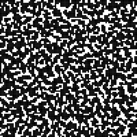
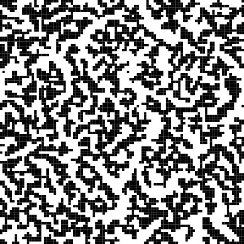
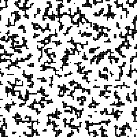
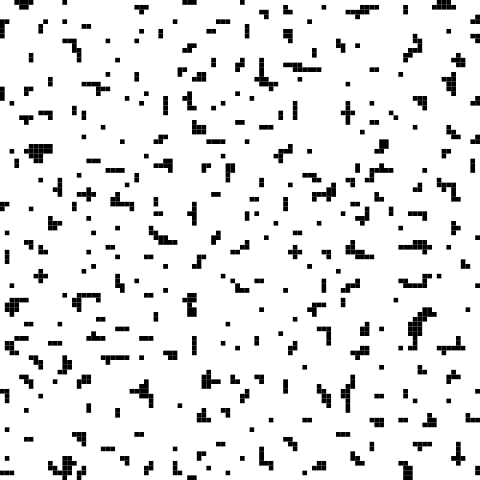
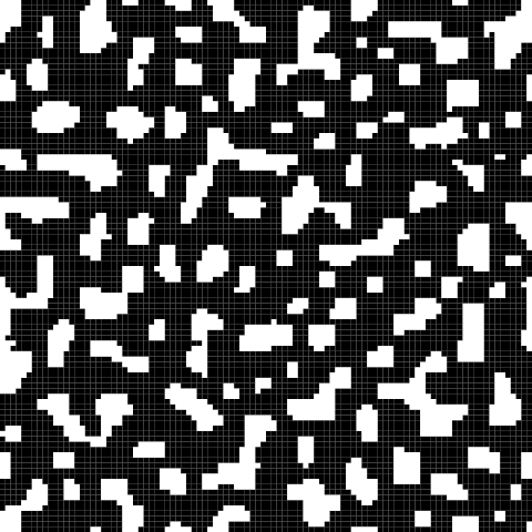
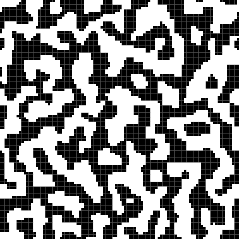
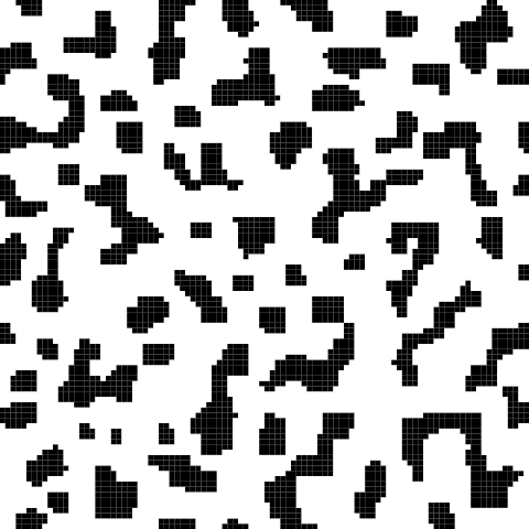
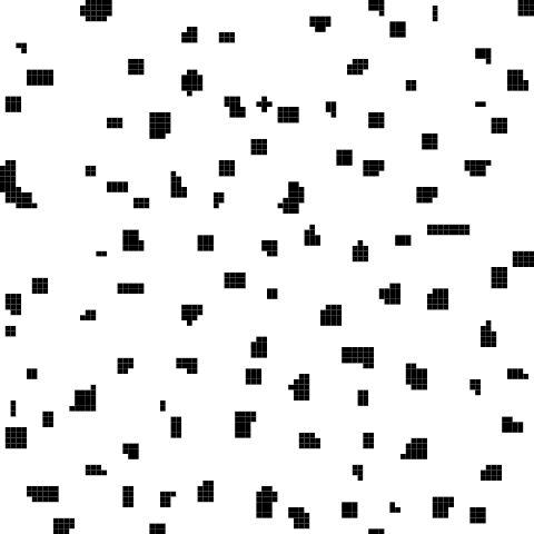
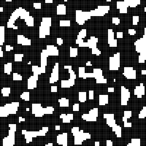
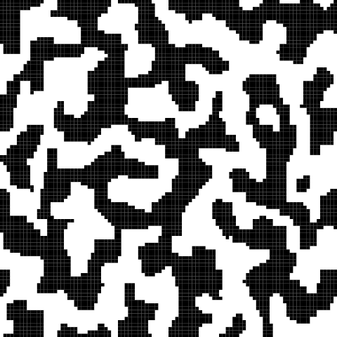
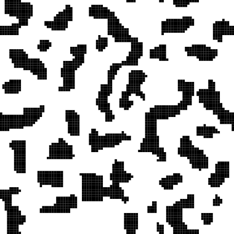
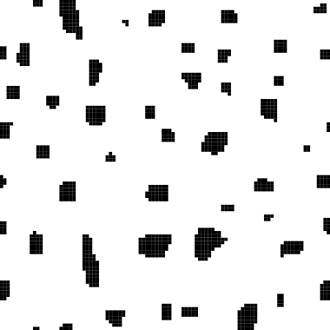
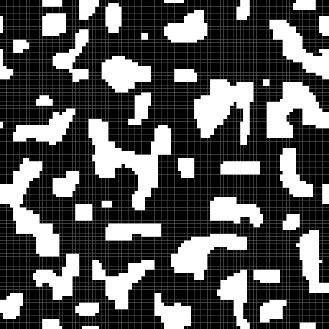
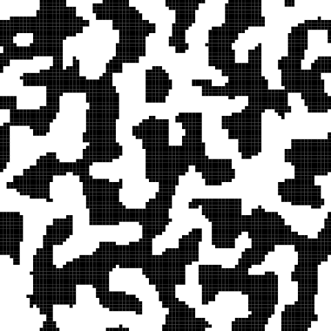
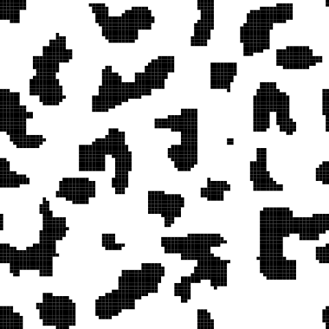
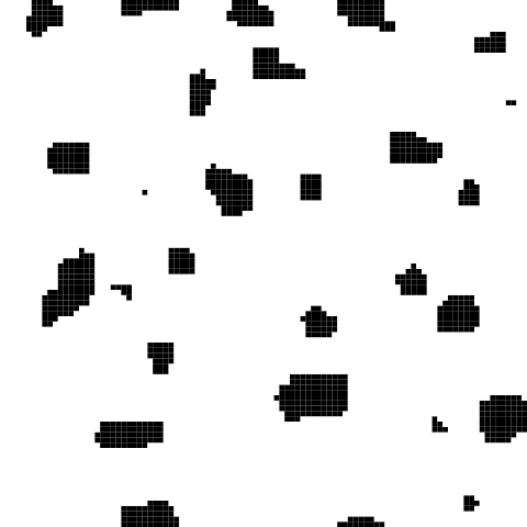
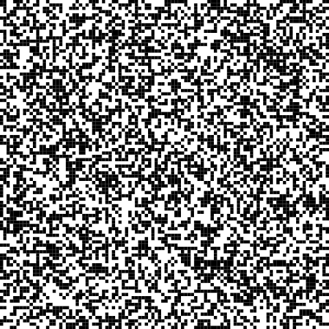
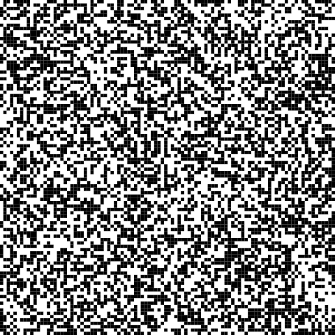
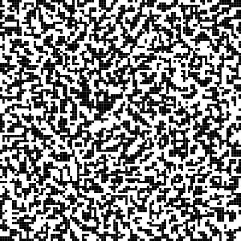
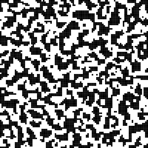
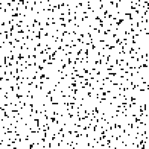
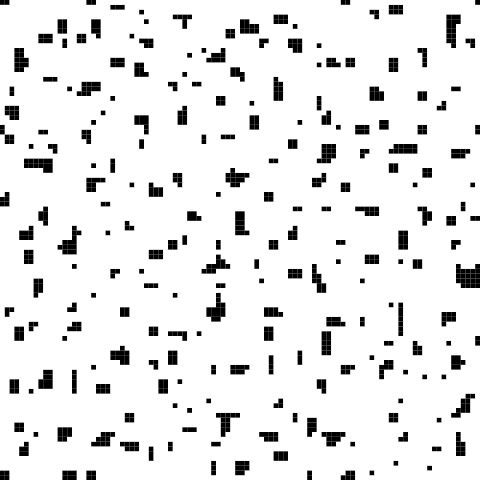
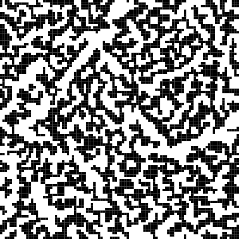
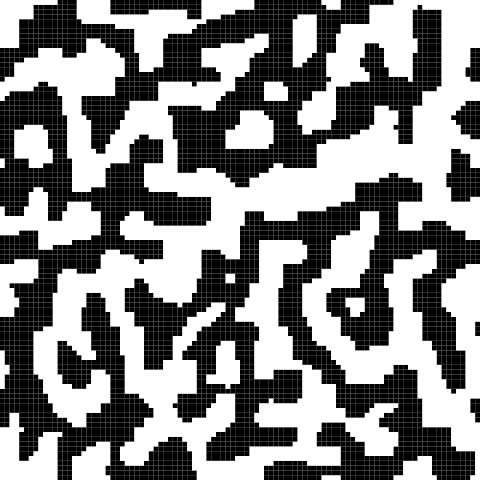
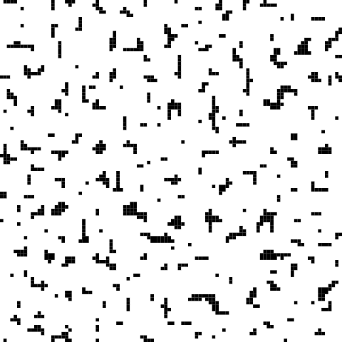
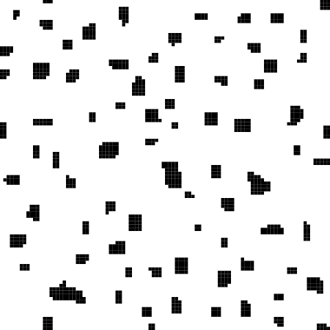
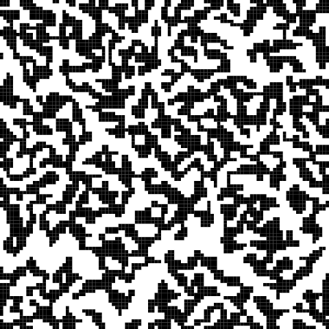
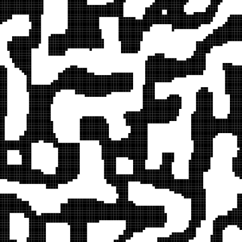
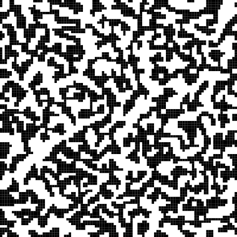
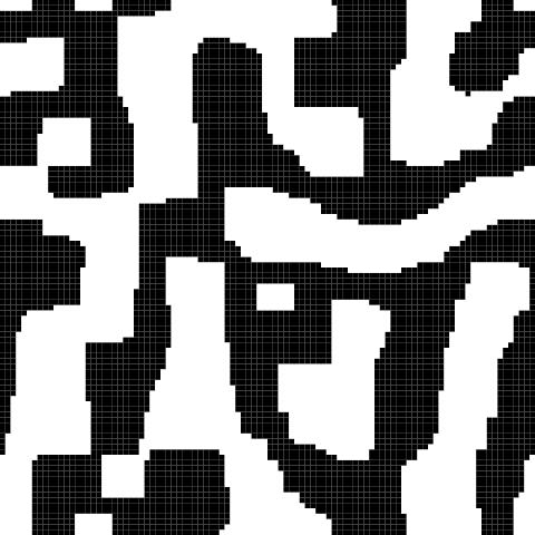
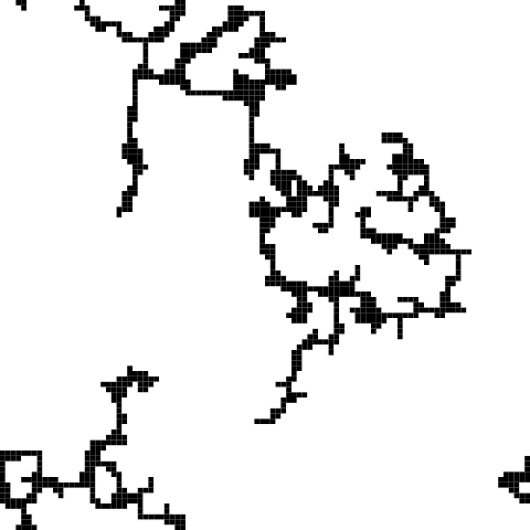
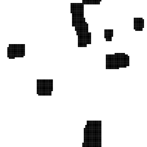
We apply the cellular automaton as introduced in Section 2.2 to illustrate the corresponding pattern formation for different choices of parameters. Starting from dispersed, randomly created structures, according to the CA jumping rules, single cells and agglomerates attract each other and finally form larger clusters and potentially also connected structures. This process is illustrated in Figure 3 for different choices of the jump parameter

$$\sigma\in\{1,5,10,15\},$$

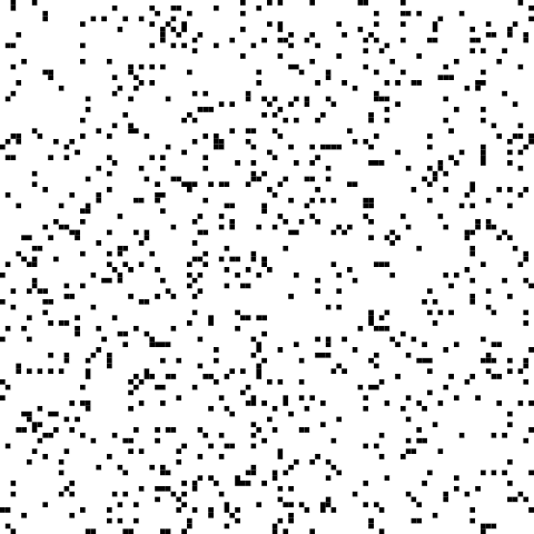
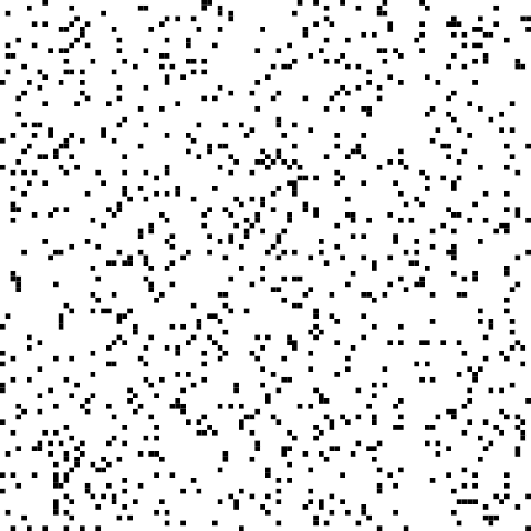
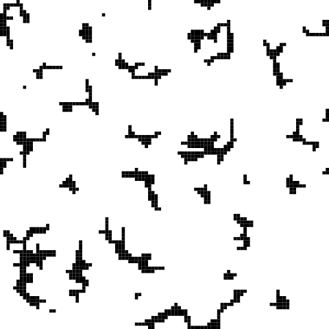
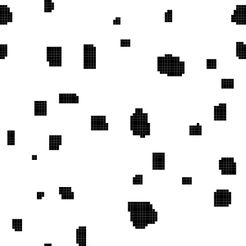
and different porosities $\theta\in\{0.3,0.5,0.7,0.9\}$. The dynamic structure development with respect to time is shown in Figure 4 for two different porosities $\theta\in\{0.5,0.9\}$ and jump parameters $\sigma\in\{1,5\}$. It is evident that distinct patterns emerge depending on the specific parameter choice. More precisely, larger porosities lead to disperse structures, while larger jump parameters lead to blocky patterns. Smaller porosities and smaller jump parameters, on the other hand, induce card-house-type structures.

		Porosity $\theta$
		0.3	0.5	0.7	0.9
Jump parameter $\sigma$	1
	5
	10
	15

Figure 3. Illustration of the domain consisting of $100\times 100$ pixels after 5 steps of the CA for varying porosity and jump parameter $\sigma$.

		$\theta=0.5$		$\theta$= 0.9
		$\sigma=1$	$\sigma=5$	$\sigma=1$	$\sigma=5$
Time step	0
	1
	5
	10
	100
	1000

Figure 4. Illustration of the time evolution of the domain consisting of $100\times 100$ pixels after steps $0,1,5,10,100$ and $1000$ of the CA for porosity $\theta\in\{0.5,0.9\}$ and jump parameter $\sigma\in\{1,5\}$.

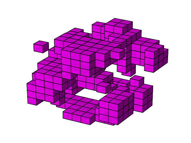
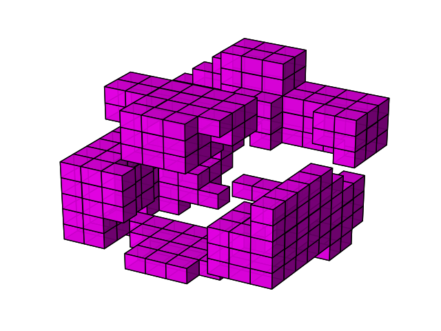
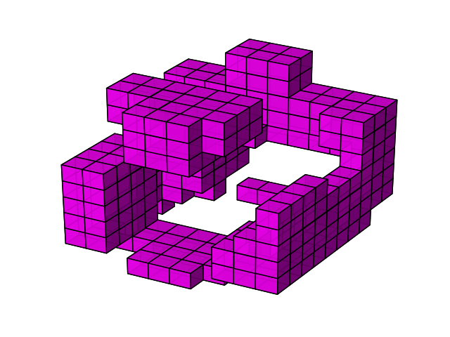
Besides the illustrations of the cellular automaton model for two spatial dimensions in Figure 3 and 4, the method can also be applied to model self organization in three spatial dimensions as shown in Figure 5. Likewise, it can also be applied in higher spatial dimensions using the implementation of [RZL22].

Timestep: 0	Timestep: 1	Timestep: 2	Timestep: 3

Figure 5. Illustration of the time evolution of the domain consisting of $10\times 10\times 10$ pixels after steps $0,1,2$ and $3$ of the CA for porosity $0.7$ and jump parameter $5$.

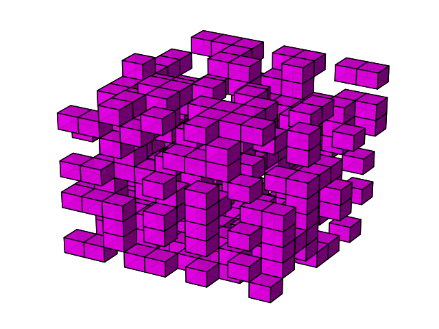The resulting patterns are used as input for further analysis by means of a parameter estimation methods as outlined below in Section 3.

3. Parameter estimation method

Figure 6. Construction and evaluation of the cost function for parameter identification by pattern data.

We now introduce the parameter estimation method which we apply to the results generated by the CA as outlined in Section 2. Our method for parameter identification allows us to map a training set of patterns to a Gaussian distribution. This in turn allows us to define a statistical likelihood and use it as a cost function during the parameter identification process. Our approach relies on emerged pattern data only, without using the information about the initial data.

3.1. Construction of the approach

Let us represent the CA model as an abstract pattern formation model depending on a vector of model parameters $\bm{\sigma}\in\mathbb{R}^{p}$. In our specific case, $\bm{\sigma}=\sigma$ is a scalar, but our method can be extended in a straight forward way to work also for a vector of parameters. We assume that the output of the “forward model” is a set of patterns $\bm{s}(\bm{\sigma})$, which is obtained by running the cellular automaton as introduced in Section 2 for various choices of the parameter(s) $\bm{\sigma}$ and a prescribed number of time steps. These patterns naturally change due to the variation of the model parameter(s), but additionally change even for fixed model parameter(s) due to the random distribution of the two phases at initial time and the randomness included in the CA steps. Our aim is to distinguish this internal variability from the systematic changes due to varying the model parameters.

More precisely, we want to find all the model parameters that fit a given training data, i.e. a set of patterns $\bm{s}_{\textup{data}}\subset\bm{s}(\bm{\sigma})$, within the accuracy allowed by the data. In order to do so, we define a minimization problem in terms of a stochastic cost function

$$f_{\bm{s}_{\textup{data}}}(\bm{\sigma})\to\min,$$ (3.1)

and consider any argument that solves (3.1) as a model parameter vector that corresponds to the training data set $\bm{s}_{\textup{data}}$. The remainder of this section is devoted to constructing $f_{\bm{s}_{\textup{data}}}$ step-by-step.

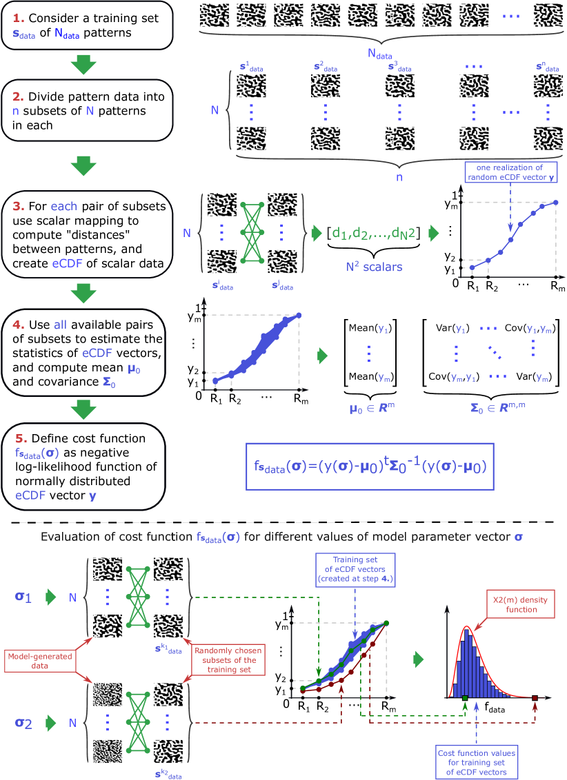
First, we specify what we mean by a solution to problem (3.1). Due to the stochasticity of the model, a given model parameter corresponds to a distribution of solutions. We thus distinguish different model parameters by the respective distributions they produce. As the pattern data is high-dimensional, we define some measure to quantify the “distance” between two samples. For this purpose, we employ the training data to construct a statistical likelihood function that quantifies the variability within the data, i.e., gives a distribution of acceptable solutions. The basic idea is to define a “distance” mapping $\rho$, e.g. a scalar mapping, which compares two patterns $\bm{s}^{+},\bm{s}^{-}$. The full statistics of $\rho$ is then used to produce a Gaussian likelihood based on/from the training data.

In order to employ the training data statistically, we divide the set of patterns into $n$ subsets. We define a function, which accepts two arguments: the sets of patterns $\bm{s}^{+}$ and $\bm{s}^{-}$ containing $N^{+}$ and $N^{-}$ patterns, respectively. This function is called empirical cumulative distribution function (eCDF), and it measures how well $\bm{s}^{+}$ and $\bm{s}^{-}$ are correlated. Apart from the two arguments, it depends on two parameters: a radius $R>0$ and the “distance” $\rho$:

$$C(\bm{s}^{+},\bm{s}^{-};R,\rho)=\frac{1}{N^{+}\times N^{-}}\sum_{i=1}^{N^{+}}\sum_{j=1}^{N^{-}}\#(\rho(\bm{s}^{+}_{i},\bm{s}^{-}_{j})<R).$$ (3.2)

The radius $R>0$ is used to create a vector $\bm{y}$ that encodes the similarity of two sets of patterns. Hence, we define a vector of bin values $(R_{i})_{i=1}^{m}$, and set

$$\bm{y}(\bm{s}^{+},\bm{s}^{-})=\bm{y}(\bm{s}^{+},\bm{s}^{-};(R_{i})_{i=1}^{m},\rho)=\left(C(\bm{s}^{+},\bm{s}^{-};R_{i},\rho)\right)_{i=1}^{m}.$$

This vector represents the eCDF of the set of values $\rho(\bm{s}^{+}_{i},\bm{s}^{-}_{j})$ evaluated at the bin values $(R_{i})_{i=1}^{m}$.

We quantify the statistics (mean and variance) of $\bm{y}(\bm{s}^{+},\bm{s}^{-})$ among subsets $\bm{s}^{+},\bm{s}^{-}$ of the whole training set $\bm{s}_{\textup{data}}$: For each subset pair, we receive $N^{2}$ scalar distance values, from which a single eCDF vector is computed. Repeating this for all distinct $n(n-1)/2$ pairs

$$\bm{y}^{k,l}=\bm{y}(\bm{s}^{k}_{\textup{data}},\bm{s}^{l}_{\textup{data}})\in\mathbb{R}^{m}\qquad 0\leq k<l\leq n,$$

we can evaluate the mean $\bm{\mu}_{0}\in\mathbb{R}^{m}$ and the covariance $\bm{\Sigma}_{0}\in\mathbb{R}^{m,m}$ of all the pairs of distinct eCDF vectors.

By the classical Donsker theorem and generalizations of it [BBD01, Neu04], finite dimensional approximations of the eCDF vectors are indeed Gaussian, in the limiting case $N\rightarrow\infty$. Since the eCDF vectors are, for high enough $N$, multinormally distributed, the mean and covariance are enough to define the statistical variability of the function $\bm{y}$ in the selected subsets of the training set. As for most applications, the normality is numerically verified here as follows: We test for Gaussianity of the ensemble of vectors using the $\chi^{2}$-test (or scalar normality tests for the components of the vector at the bin values). For this purpose, we evaluate all the values of the negative log-likelihood function

$$(\bm{y}^{k,l}-\bm{\mu}_{0})^{T}\bm{\Sigma}_{0}^{-1}(\bm{y}^{k,l}-\bm{\mu}_{0}),$$

and compare the resulting histogram against the density function of the distribution $\chi^{2}_{M}$ with $m$ degrees of freedom.

To evaluate the cost function at a new parameter value $\bm{\sigma}$, we simulate the CA model $N$ times using $\bm{\sigma}$ and denote the collection of patterns by $\bm{s}(\bm{\sigma})$. The eCDF vector $\bm{y}(\bm{\sigma})=\bm{y}(\bm{s}(\bm{\sigma}),\bm{s}^{k}_{\textup{data}})$ can then be computed for one randomly selected $k\in\{1,2,\dots,n\}$, and the likelihood value is evaluated as

$$f_{\bm{s}_{\textup{data}}}(\bm{\sigma})=(\bm{y}(\bm{\sigma})-\bm{\mu}_{0})^{T}\bm{\Sigma}_{0}^{-1}(\bm{y}(\bm{\sigma})-\bm{\mu}_{0}).$$

3.2. Numerical implementation

3.2.1. Choice of bins

The bin values for the eCDF vectors can be selected in various ways. Here we use the following approach: We first use the first two subsets of the training data and determine the minimum and maximum of the function $C$ as defined in (3.2) (with respect to $R$). Next, we uniformly split the respective interval into $50$ possible bin values. This allows us to represent the shape of the eCDF curve. However, in numerical application such dense coverage might result in unwanted correlation between neighbouring bin values. Therefore, from these preliminary bins we choose a smaller subset of $n_{bin}$ values, which we select by an inverse CDF method: to get the bin values on the x-axis, a set of $n_{bin}$ linearly spaced values on the y-axis are mapped to the x-axis by the inverse CDF (quantile) function, using the mean of the preliminary CDF vectors. Additionally, a cut-off parameter of $0.1$ is used to step away from boundaries of the range $[0,1]$ of the CDF function. This allows us to exclude bins with possibly prohibitively small variabilities, which might result in singularities in the covariance matrix of the underlying Gaussian distribution. Thereafter the Gaussianity of both configurations of bins (the preliminary and the selected sparse one) can be evaluated.

3.2.2. Choice of characteristics

The algorithm of [KSHMC22] employs several norms to characterize the distance between two patterns in the situation of continuous-valued images. As the present setting is discrete, with binary-valued patterns, we use the $L^{1}$-norm, i.e. we define the distance function $\rho(\bm{s},\bm{\hat{s}})=\|\bm{s}^{+}-\bm{s}^{-}\|_{L^{1}}$ between two patterns $\bm{s}^{+},\bm{s}^{-}$.

However, for the discrete CA patterns, various other candidates for a characteristics are reasonable. Here, exemplary, we use the particle size distribution or the average particle size. The average particle size is the mean of the particle size distribution, i.e. it is defined as the arithmetic average of the sizes of all particles, i.e. single cells and agglomerates. As our approach is based on the statistical distribution of the CDF functions of scalar data, we can also employ the particle size distribution directly, by forming the empirical CDF of it. Although the particle size distribution could be computed for each pattern separately, we compute the particle size distributions of all pairwise combinations of patterns. This has the advantage of producing more eCDF vectors, which stabilizes the numerical estimation of the mean and covariance of the likelihood.

3.2.3. Application of the eCDF method to the base setup

We perform numerical experiments to demonstrate how our parameter estimation method can be applied to identify parameters of the CA model from synthetic (model-generated) data. We first consider a basic experimental setup, which is defined as follows:

• The CA is run on a two-dimensional domain of size $50\times 50$ with porosity $\theta=0.7$ and jump parameter $\sigma=5$.

• The training set of patterns is obtained by running 5 iterations of the CA model with random initial data (4000 = 40$\times$100 realisations).

For this basic experimental setup, we begin with creating the $L^{1}$ likelihood and estimating the model parameters using the $L^{1}$-norm.

Figure 7. Construction of the statistical likelihood for basic experimental setup and its evaluation for different values of jump parameter $\sigma$. Top left: distribution of the eCDF curves for dense bin values (purple) and selected bins only (light blue). Here, black dots denote the respective mean values of eCDF vectors over all available pairs. Bottom left: Gaussianity test by $\chi^{2}$ criterion for selected bin values. Top right: repetitive evaluation of the negative log-likelihood (cost function) for integer values of jump parameter $\sigma$ on the interval $[0,10]$. Here, cost function values are plotted by red color, while blue dots denote the average over all evaluations. Bottom right: normalized likelihood values (red) and averaged values over evaluations (blue).

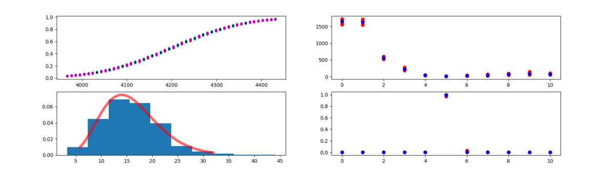
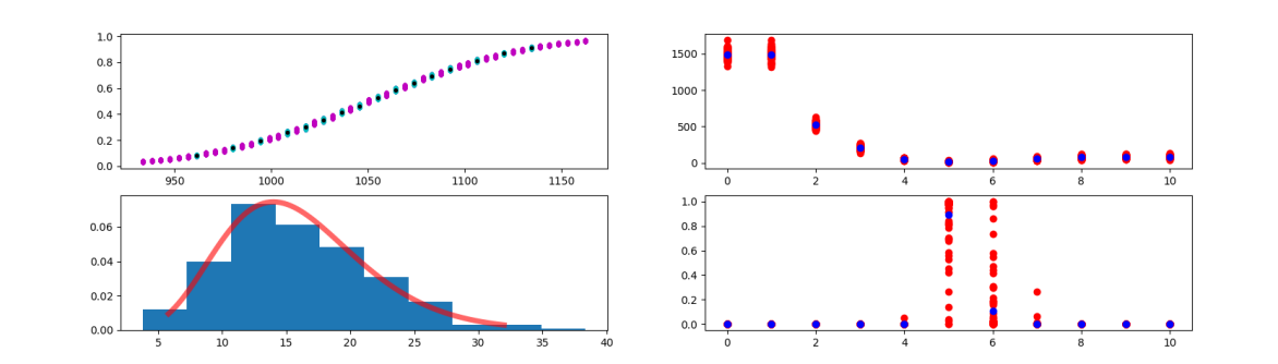
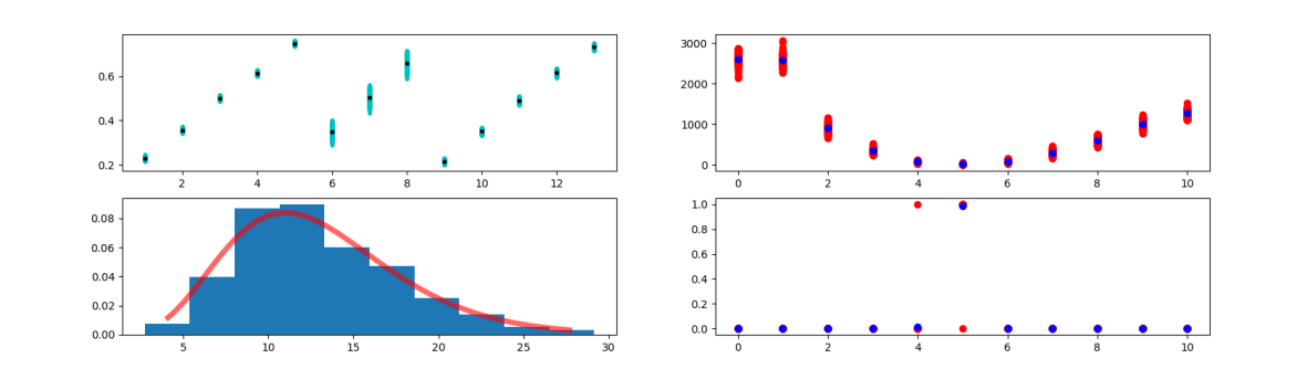
Following the procedure outlined in Section 3 and illustrated in Figure 6, we create a statistical likelihood from the training data. We split the training set into 40 subsets with 100 samples in each. Next, for every pair, we compute distances between the respective patterns in terms of $L^{1}$-norm, and compute the eCDF of the respective scalar data. Here, we successively select bins for the eCDF vectors by using the algorithm described in Section 3.2.1. The selection is illustrated in Figure 7 (top left).

Next, we check the Gaussianity of the selected bins as outlined in Section 3, which is illustrated in the bottom left part of the Figure 7. We evaluate the negative log-likelihood for integer values of the jump parameter $\sigma$ on the interval $[0,10]$, as is shown in Figure 7 (top right). Here, the red dots represent the evaluation of this value 100 times and the blue dots highlight the averare values of the red dots We observe, that the minimum of the negative log likelihood values is achieved at $\sigma=5$. Finally, the proper probabilistic interpretation is obtained by the normalized likelihood values in Figure 7 (bottom right)—with the same interpretation of red and blue dots. Thus our approach is capable to properly distinguish patterns, corresponding to different values of $\sigma$ for this setup.

4. Results

Next, we investigate the robustness of the parameter estimation method as introduced in Section 3 with respect to number of bins, the domain size, and the number of time steps (iterations) in the CA model. Here, we change only one quantity at a time, while the other ones are fixed to the default values as prescribed by the basic experimental setup in the previous Section. Finally, we analyze the impact of including additional CA-specific characteristics to the scheme of the parameter estimation method, which is discussed in Section 4.4.

4.1. Varying number of bins

We first study the robustness of our parameter estimation method with respect to the number of selected bins (dimension of eCDF vectors). We repeat the experiments described in Section 3.2.3 for a varying number of bins between 6 and 26, while keeping the other parameters fixed. The results were statistically identical to the ones shown in Figure 7 for all considered cases. From this result we conclude that the approach allows for a quite large flexibility with respect to the number of bins, once the considerations about numerical stability, discussed in Section 3.2.1 are taken into account.

((a))

((b))

((c))

Figure 8. Construction of the statistical likelihood for various domain sizes and its evaluation for different values of jump parameter $\sigma$. The layout of sub-figures is identical to Figure 7.

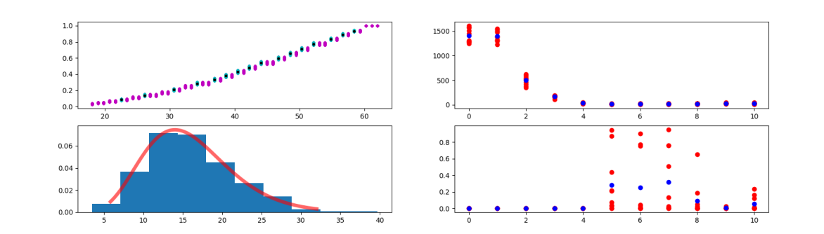
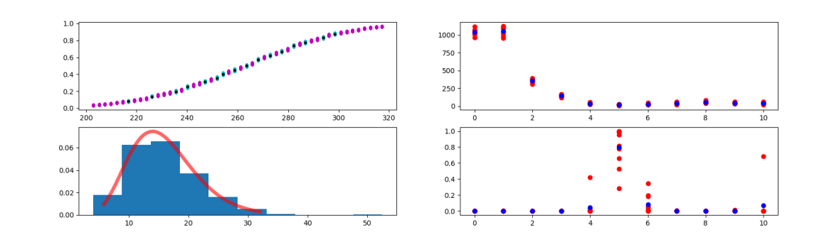
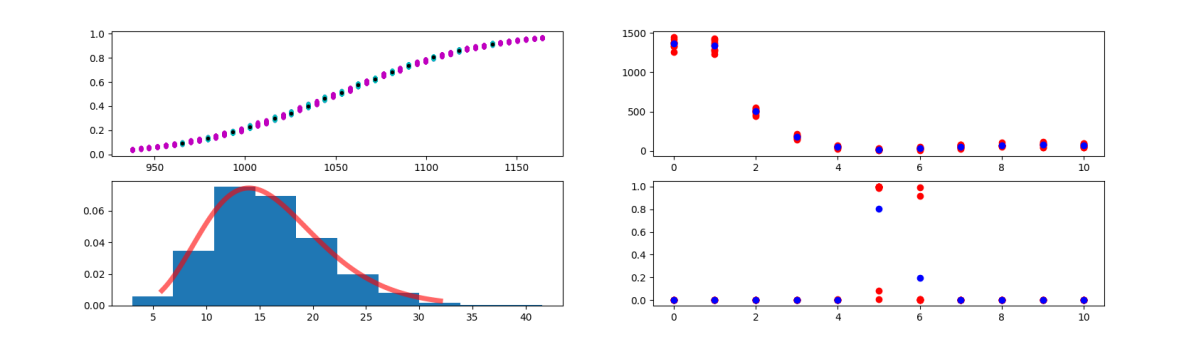
4.2. Varying domain sizes

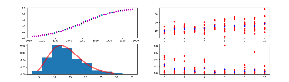
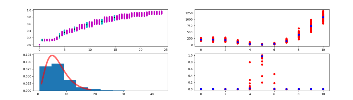
We now consider different domain sizes, i.e. we perform the procedure of Section 3.2.3 for domains of size $10\times 10$, $25\times 25$, and $100\times 100$. Obviously, a simulation that is conducted on a small domain provides less information than a simulation that is conducted on a large domain, but keeping the porosity fixed. This is underpinned by the numerical experiments illustrated in Figure 8.

Considering first the $10\times 10$ domain, our algorithm is able to correctly identify the true parameter $\sigma=5$. The minimum, however, is not very pronounced, which means that the accuracy is quite low. For domain sizes of $25\times 25$, $50\times 50$ (basic experimental setup, see Figure 7), and $100\times 100$, we observe again smooth eCDF shapes, thus the parameter estimation method works accurately and successfully. The increase in domain size leads to a more pronounced minimum at $\sigma=5$. Thus, the algorithm is more certain to identify the correct jump parameter if the domain size, and thereby the available amount of information, is increased.

((a))

((b))

((c))

((d))

Figure 9. Construction of the statistical likelihood for various numbers of CA iterations, and its evaluation for different values of jump parameter $\sigma$. The layout of sub-figures is identical to Figure 7.

4.3. Varying number of CA iterations

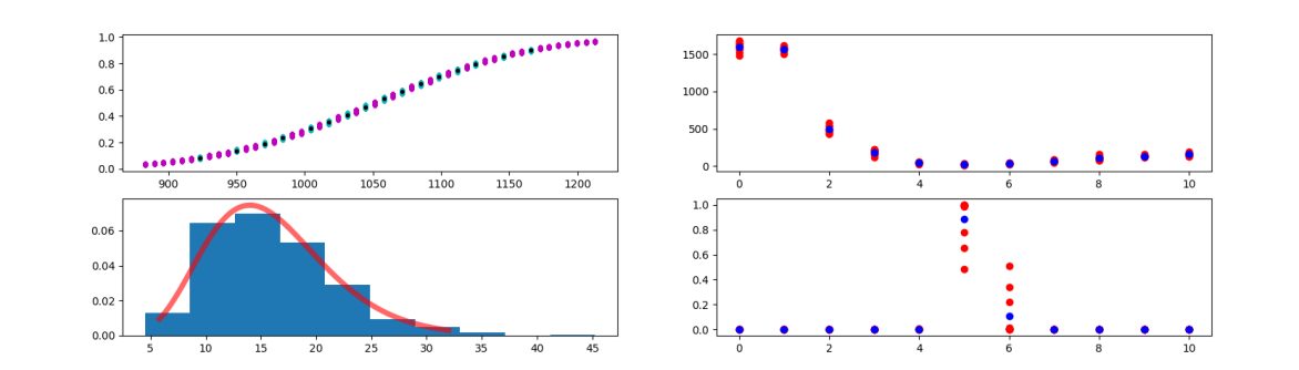
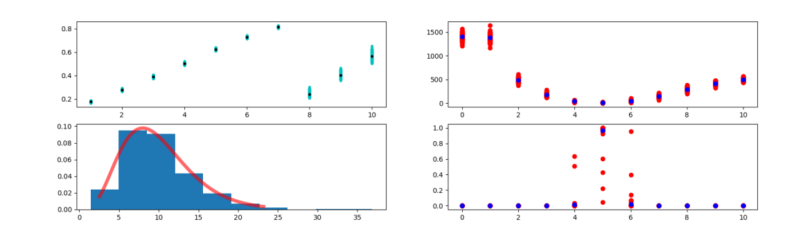
The patterns, generated by our CA model, are not stationary since initially fragmented particles eventually attract each other and self-organize into larger, connected structures. Thus, depending on how many model iterations were used to create a pattern, it can be more or less clustered, see also illustration in Figure 4. Here, we study how this factor affects our ability to perform the parameter identification. The results are illustrated in Figure 9. We start from considering the trivial case of zero iterations. In this case, the disperse initial state is independent of $\sigma$ and thus we can construct the likelihood without any problems, but we naturally cannot detect any difference between different values of $\sigma$. However, the parameter identification works without issues for all other considered cases: $1$, $5$ (base experimental setup, see Figure 7), $10$, $25$, or $50$ iterations. This indicates that the number of iterations does not significantly influence the quality of our parameter estimation method.

((a))

((b))

((c))

((d))

((e))

Figure 10. Construction of the statistical likelihood for multiple characteristics in parameter estimation method, and its evaluation for different values of jump parameter $\sigma$. The layout of sub-figures is identical to Figure 7.

4.4. Multiple features in parameter estimation method

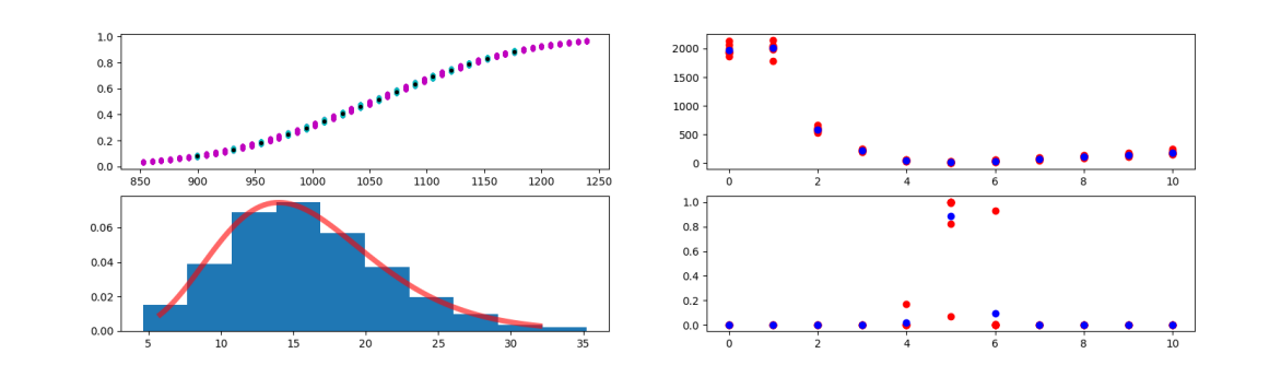
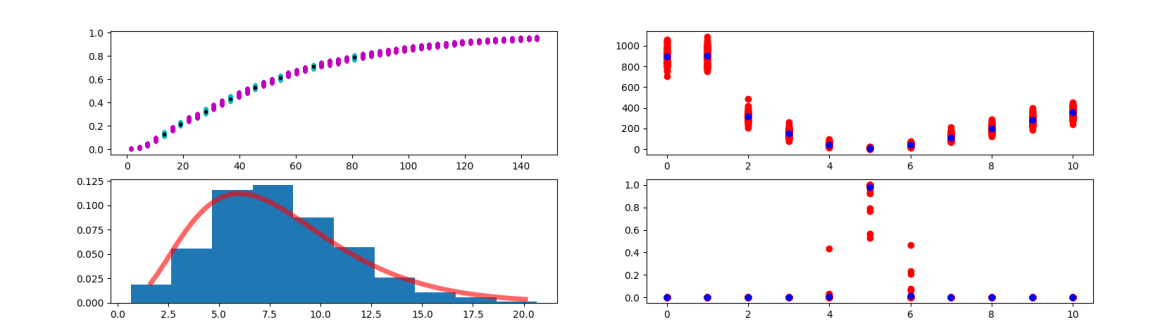
In this section, we again consider the basic experimental setup and discuss how the parameter identification procedure can be improved by taking into account additional features, typical for characterizing structures of CA models as outlined in Section 3. Computing the distance between pattern data using $L^{1}$-norm allowed us to correctly identify the correct value of jump parameter $\sigma$ (see Figure 10 (A)), however, the minimum of the cost function is not always well pronounced. This may result in higher uncertainty in parameter identification, and can be seen from the wide spread of the red dots. We can, however, significantly reduce the uncertainty by additionally using the characteristics introduced in Section 3.

The first feature we use here is the average particle size. This means that instead of computing the $L^{1}$-distance between two patterns, we use the absolute difference of the respective average particle sizes. We observe that if we replace the $L^{1}$-distance with this new mapping, the variability of the cost function is nicely reduced and the minimum becomes more pronounced (see Figure 10 (B)). An even better effect, however, can be achieved by combining this characterisitcs with the previously used $L^{1}$-distance (see Figure 10 (C)). Since concatenation of the respective eCDF vectors is again Gaussian, the same approach as before can be applied directly.

Next, we consider a different mapping from a pair of subsets of pattern data to one eCDF vector. That is, we do not use a distance that produces a scalar from a pair of patterns, but directly create a distribution that holds the information of several scalars. Here, we employ the fact that an eCDF vector is directly available, in the form of the particle size distribution of each CA pattern. Thus, we pool together the particles sizes from each pair of pattern subsets (each containing $N$ patterns) and construct one eCDF vector of all the emerging scalar values. This gives us a large amount of scalar data, which results in a smooth eCDF curves. Again, all the pairs yield $n(n-1)/2$ eCDF curves. This gives us another separate feature for the parameter estimation (see Figure 10 (D)). Naturally, the best results are obtained when all those features are taken together. This case is shown in Figure 10 (E). Especially, we observe the minimal variability of the cost function.

5. Conclusions

In this work, we introduced a parameter identification which works well for discrete problems as in the context of CA models. Our parameter estimation method allowed to perform model parameter identification using pattern data only, without any knowledge about initial states. We demonstrated the applicability of the method by successfully identifying the value of jump parameter $\sigma$ from a set of $4000$ patterns. Moreover, we proved the robustness of our approach for different configurations of the model with respect to the number of selected bins, the domain size and the number of CA steps. Finally, we showed that the accuracy could be drastically improved if commonly used features of the CA pattern data were incorporated into the scheme of our method.

Future work may include an application of the parameter estimation method to more than one parameter as already outlined in [HKH15], as well as in combination of various characteristics/norms.

Additionally, more sophisticated cellular automaton models may be used. Along this lone realistic problems could be addressed, the underlying process understanding could be improved and conclusions relevant for real-life problems could be drawn.

References

- [AMR+19] R. Armstrong, J. Mcclure, V. Robins, Z. Liu, C. Arns, S. Schlüter, and S. Berg. Porous media characterization using Minkowski functionals: Theories, applications and future directions. Transport in Porous Media, 130, 10 2019. 10.1007/s11242-018-1201-4.
- [BBD01] S. Borovkova, R. Burton, and H. Dehling. Limit theorems for functionals of mixing processes with applications to u-statistics and dimension estimation. Trans. AMS, 353:4261–4318, 2001.
- [CK10] E. Couce and W. Knorr. Statistical parameter estimation for a cellular automata wildfire model based on satellite observations. WIT Transactions on Ecology and the Environment, 137:47–55, 2010.
- [GMC+17] P. Ghosh, A. Mukhopadhyay, A. Chanda, P. Mondal, A. Akhand, S. Mukherjee, S.K. Nayak, S. Ghosh, D. Mitra, T. Ghosh, et al. Application of cellular automata and markov-chain model in geospatial environmental modeling-a review. Remote Sensing Applications: Society and Environment, 5:64–77, 2017.
- [HKH15] H. Haario, L. Kalachev, and J. Hakkarainen. Generalized correlation integral vectors: A distance concept for chaotic dynamical systems. Chaos, 25(6), 2015. 10.1063/1.4921939.
- [KH20] A. Kazarnikov and H. Haario. Statistical approach for parameter identification by Turing patterns. Journal of Theoretical Biology, 501:110319, 05 2020. 10.1016/j.jtbi.2020.110319.
- [KSHMC22] A. Kazarnikov, R. Scheichl, H. Haario, and A. Marciniak-Czochra. A Bayesian approach to modelling biological pattern formation with limited data, 2022. https://arxiv.org/abs/2203.14742.
- [LYL07] X. Li, Q.S. Yang, and X.P. Liu. Genetic algorithms for determining the parameters of cellular automata in urban simulation. Science in China Series D: Earth Sciences, 50(12):1857–1866, 2007.
- [MD02] J. Moreira and A. Deutsch. Cellular automaton models of tumor development: a critical review. Advances in Complex Systems, 5(02n03):247–267, 2002.
- [MKL20] N. Menshutina, A. Kolnoochenko, and E. Lebedev. Cellular automata in chemistry and chemical engineering. Annual Review of Chemical and Biomolecular Engineering, 11:87–108, 2020.
- [Neu04] N. Neumeyer. A central limit theorem for two-sample u-processes. Statistics & Probability Letters, 67(1):73 – 85, 2004. doi.org/10.1016/j.spl.2002.12.001.
- [RGK22] A. Rupp, M. Gahn, and G. Kanschat. Partial differential equations on hypergraphs and networks of surfaces: Derivation and hybrid discretizations. ESAIM: Mathematical Modelling and Numerical Analysis, 56(2):505–528, 2022. 10.1051/m2an/2022011.
- [RHK22] A. Rupp, H. Haario, and A. Kazarnikov. ECDF estimator: Python implementation for parameter estimation based on correlation integral likelihoods and empirical cumulative distribution functions, 2022. https://github.com/AndreasRupp/ecdf_estimator. published online.
- [RK21] A. Rupp and G. Kanschat. HyperHDG: Hybrid discontinuous Galerkin methods for PDEs on hypergraphs, 2021. https://github.com/HyperHDG. published online.
- [RRP17] N. Ray, A. Rupp, and A. Prechtel. Discrete-continuum multiscale model for transport, biomass development and solid restructuring in porous media. Advances in Water Resources, 107:393–404, 2017. 10.1016/j.advwatres.2017.04.001.
- [RZL22] A. Rupp, S. Zech, and J. Lappalainen. Cellular automaton: C++ implementation of a simple cellular automaton method, 2022. https://github.com/AndreasRupp/cellular-automaton. published online.
- [SGMC10] I. Santé, A. García, D. Miranda, and R. Crecente. Cellular automata models for the simulation of real-world urban processes: A review and analysis. Landscape and urban planning, 96(2):108–122, 2010.
- [TZJT21] J. Tian, C. Zhu, R. Jiang, and M. Treiber. Review of the cellular automata models for reproducing synchronized traffic flow. Transportmetrica A: Transport Science, 17(4):766–800, 2021.
- [XWC11] X. Xiao, P. Wang, and K.-C. Chou. Cellular automata and its applications in protein bioinformatics. Current Protein and Peptide Science, 12(6):508–519, 2011.
- [YWLF11] H. Yang, C. Wu, H.W. Li, and X.G. Fan. Review on cellular automata simulations of microstructure evolution during metal forming process: Grain coarsening, recrystallization and phase transformation. Science China Technological Sciences, 54(8):2107–2118, 2011.
- [YX04] A. Yeh and L. Xia. Integration of neural networks and cellular automata for urban planning. Geo-spatial Information Science, 7(1):6–13, 2004. 10.1007/BF02826669.
- [ZSB+22] S. Zech, S. A. Schweizer, F. B. Bucka, N. Ray, I. Kögel-Knabner, and A. Prechtel. Explicit spatial modeling at the pore scale unravels the interplay of soil organic carbon storage and structure dynamics. Global Change Biology, 2022. 10.1111/gcb.16230.