A Safety Framework for Flow Decomposition Problems via Integer Linear Programming

Abstract

Many important problems in Bioinformatics (e.g., assembly or multi-assembly) admit multiple solutions, while the final objective is to report only one. A common approach to deal with this uncertainty is finding safe partial solutions (e.g., contigs) which are common to all solutions. Previous research on safety has focused on polynomially-time solvable problems, whereas many successful and natural models are NP-hard to solve, leaving a lack of “safety tools” for such problems. We propose the first method for computing all safe solutions for an NP-hard problem, minimum flow decomposition. We obtain our results by developing a “safety test” for paths based on a general Integer Linear Programming (ILP) formulation. Moreover, we provide implementations with practical optimizations aimed to reduce the total ILP time, the most efficient of these being based on a recursive group-testing procedure.
Results: Experimental results on the transcriptome datasets of Shao and Kingsford (TCBB, 2017) show that all safe paths for minimum flow decompositions correctly recover up to 90% of the full RNA transcripts, which is at least 25% more than previously known safe paths, such as (Cáceres et al. TCBB, 2021), (Zheng et al., RECOMB 2021), (Khan et al., RECOMB 2022, ESA 2022). Moreover, despite the NP-hardness of the problem, we can report all safe paths for 99.8% of the over 27,000 non-trivial graphs of this dataset in only 1.5 hours. Our results suggest that, on perfect data, there is less ambiguity than thought in the notoriously hard RNA assembly problem.
Availability: https://github.com/algbio/mfd-safety
Contact: alexandru.tomescu@helsinki.fi

1 Introduction

In real-world scenarios where an unknown object needs to be discovered from the input data, we would like to formulate a computational problem loosely enough so that the unknown object is indeed a solution to the problem, but also tightly enough so that the problem does not admit many other solutions. However, this goal is difficult in practice, and indeed, various commonly used problem formulations in Bioinformatics still admit many solutions. While a naive approach is to just exhaustively enumerate all these solutions, a more practical approach is to report only those sub-solutions (or partial solutions) that are common to all solutions to the problem.

In the graph theory community such sub-solutions have been called persistent [14, 21], and in the Bioinformatics community reliable [54], or more recently, safe [51]. The study of safe sub-solutions started in Bioinformatics in the 1990’s [54, 11, 37] with those amino-acid pairs that are common to all optimal and suboptimal alignments of two protein sequences.

In the genome assembly community, the notion of contig, namely a string that is guaranteed to appear in any possible assembly of the reads, is at the core of most genome assemblers. This approach originated in 1995 with the notion of unitigs [25] (non-branching paths in an assembly graph), which were progressively [42, 6] generalized to paths made up of a prefix of nodes with in-degree one followed by nodes with out-degree one [35, 24, 29] (also called extended unitigs, or Y-to-V contigs).

Later, [51] formalized all such types of contigs as those safe strings that appear in all solutions to a genome assembly problem formulation, expressed as a certain type of walk in a graph. [10, 9] proposed more efficient and unifying safety algorithms for several types of graph walks. [45] recently studied the safety of contigs produced by state-of-the-art genome assemblers on real data.

Analogous studies were recently made also for multi-assembly problems, where several related genomic sequences need to be assembled from a sample of mixed reads. [8] studied safe paths that appear in all constrained path covers of a directed acyclic graph (DAG). Zheng, Ma and Kingsford studied the more practical setting of a network flow in a DAG by finding those paths that appear in any flow decomposition of the given network flow, under a probabilistic framework [34], or a combinatorial framework [58]. [27] presented a simple characterization of safe paths appearing in any flow decomposition of a given acyclic network flow, leading to a more efficient algorithm than the one of [58], and further optimized by [28].

Motivation.

Despite the significant progress in obtaining safe algorithms for a range of different applications, current safe algorithms are limited to problems where computing a solution itself is achievable in polynomial time. However, many natural problems are NP-hard, and safe algorithms for such problems are fully missing. Apart from the theoretical interest, usually such NP-hard problems correspond to restrictions of easier (polynomially-computable) problems, and thus by definition, also have longer safe sub-solutions.

As such, current safety algorithms miss data that could be reported as correct, just because they do not constrain the solution space enough. A major reason for this lack of progress is that if a problem is NP-hard, then its safety version is likely to be hard too. This phenomenon can be found both in classically studied NP-hard problems — for example, computing nodes present in all maximum independent sets of an undirected graph is NP-hard [21] — as well as in NP-hard problems studied for their application to Bioinformatics, as we discuss further in the appendix.

We introduce our results by focusing on the flow decomposition problem. This is a classical model at the core of multi-assembly software for RNA transcripts [33, 31, 5, 50] and viral quasi-species genomes [3, 2, 44, 12], and also a standard problem with applications in other fields, such as networking [36, 22, 13, 23] or transportation [39, 38]. In its most basic optimization form, minimum flow decomposition (MFD), we are given a flow in a graph, and we need to decompose it into a minimum number of paths with associated weights, such that the superposition of these weighted paths gives the original flow. This is an NP-hard problem, even when restricted to DAGs [53, 22]. Various approaches have been proposed to tackle the problem, including fixed-parameter tractable algorithms [30], approximation algorithms [36, 7] and Integer Linear Programming formulations [15, 46].

In Bioinformatics applications, reads or contigs originating from a mixed sample of genomic sequences with different abundances are aligned to a reference. A graph model, such as a splice graph or a variation graph, is built from these alignments. Read abundances assigned to the nodes and edges of this graph then correspond to a flow in case of perfect data. If this is not the case, the abundance values can either be minimally corrected to become a flow, or one can consider variations of the problem where e.g., the superposition of the weighted paths is closest (or within a certain range) to the edge abundances [50, 5].

Current safety algorithms for flow decompositions such as [58, 27, 26, 28] compute paths appearing in all possible flow decompositions (of any size), even though decompositions of minimum size are assumed to better model the RNA assembly problem [30, 48, 55]. Even dropping the minimality constraint, but adding other simple constraints easily renders the problem NP-hard (see e.g., [56]), motivating further study of practical safe algorithms for NP-hard problems.

Contributions.

Integer Linear Programming (ILP) is a general and flexible method that has been successfully applied to solve NP-hard problems, including in Bioinformatics. In this paper, we consider graph problems whose solution consists of a set of paths (i.e., not repeating nodes) that can be formulated in ILP. We introduce a technique that, given an ILP formulation of such a graph problem, can enhance it with additional variables and constraints in order to test the safety of a given set of paths. An obvious first application of this safety test is to use it with a single path in a straightforward avoid-and-test approach, using a standard two-pointer technique that has been used previously to find safe paths for flow decomposition. However, we find that a top-down recursive approach that uses the group-testing capability halves the number of computationally-intensive ILP calls, resulting in a 3x speedup over the straightforward approach.

Additionally, we prove that computing all the safe paths for MFDs is an intractable problem, confirming the above intuitive claim that if a problem is hard, then also its safety version is hard. We give this proof in the appendix by showing that the NP-hardness reduction for MFD by [22] can be modified into a Turing reduction from the UNIQUE 3SAT problem.

On the dataset [47] containing splice graphs from human, zebrafish and mouse transcriptomes, safe paths for MFDs (SafeMFD) correctly recover up to 90% of the full RNA transcripts while maintaining a 99% precision, outperforming, by a wide margin (25% increase), state-of-the-art safety approaches, such as extended unitigs [35, 24, 29], safe paths for constrained path covers of the edges [8], and safe paths for all flow decompositions [28, 27, 26, 58]. On the harder dataset by [26], SafeMFD also dominates in a significant proportion of splice graphs (built from $t\leq 15$ RNA transcripts), recovering more than 95% of the full transcripts while maintaining a 98% precision. For larger $t$, precision drastically drops (91% precision in the entire dataset), suggesting that in more complex splice graphs smaller solutions are introduced as an artifact of the combinatorial nature of the splice graph, and the minimality condition [30, 48, 55] is thus incorrect in this domain.

2 Methods

2.1 Preliminaries

ILP models.

In this paper we use ILP models as blackboxes, with as few assumptions as possible to further underline the generality of our approach. Let $\mathcal{M}(\mathcal{V},\mathcal{C})$ be an ILP model consisting of a set $\mathcal{V}$ of variables and a set $\mathcal{C}$ of constraints on these variables, built from an input graph $G=(V,E)$. We make only two assumptions on $\mathcal{M}$. First, that a solution to this model consists of a given number $k\geq 1$ of paths $P_{1},\dots,P_{k}$ in $G$ (in this paper, paths do not repeat vertices). Second, we assume that the $k$ paths are modeled via binary edge variables $x_{uvi}$, for all $(u,v)\in E$ and for all $i\in\{1,\dots,k\}$. More specifically, for all $i\in\{1,\dots,k\}$, we require that the edges $(u,v)\in E$ for which the corresponding variable $x_{uvi}$ equals 1 induce a path in $G$. For example, if $G$ is a DAG, it is a standard fact (see e.g., [49]) that a path from a given $s\in V$ to a given $t\in V$ (an $s$-$t$ path) can be expressed with the following constraints:

$$\sum_{(u,v)\in E}x_{uvi}-\sum_{(v,u)\in E}x_{vui}=\begin{cases}0,&\text{if $v\in V\setminus\{s,t\}$},\\ 1,&\text{if $v=t$},\\ -1,&\text{if $v=s$}.\end{cases}$$ (1)

If $G$ is not a DAG, there are other types of constraints that can be added to the $x_{uvi}$ variables to ensure that they induce a path; see, for example, the many formulations in [49]. We will assume that such constraints are part of the set $\mathcal{C}$ of constraints of $\mathcal{M}(\mathcal{V},\mathcal{C})$, but their exact formulation is immaterial for our approach. In fact, one could even add additional constraints to $\mathcal{C}$ to further restrict the solution space. For example, some ILP models from [15, 46] handle the case when the input also contains a set of paths (subpath constraints) that must appear in at least one of the $k$ solution paths.

Flow decomposition.

In the flow decomposition problem we are given a flow network $(V,E,f)$, where $G=(V,E)$ is a (directed) graph with unique source $s\in V$ and unique sink $t\in V$, and $f$ assigns a positive integer flow value $f_{uv}$ to every edge $(u,v)\in E$. Flow conservation must hold for every node different from $s$ and $t$, namely, the sum of the flow values entering the node must equal the sum of the flow values exiting the node. See Figure 1(a) for an example. We say that $k$ $s$-$t$ paths $P_{1},\dots,P_{k}$, with associated positive integer weights $w_{1},\dots,w_{k}$, are a flow decomposition (FD) if their superposition equals the flow $f$. Formally, for every $(u,v)\in E$ it must hold that

$$\sum_{\begin{subarray}{c}i\in\{1,\dots,k\}\text{ s.t. }\\ (u,v)\in P_{i}\end{subarray}}w_{i}=f_{uv}.$$ (2)

See Figures 1(b) and 1(c) for two examples. The number $k$ of paths is also called the size of the flow decomposition. In the minimum flow decomposition (MFD) problem, we need to find a flow decomposition of minimum size. On DAGs, a flow decomposition into paths always exists [1], but in general graphs, cycles may be necessary to decompose the flow (see e.g. [16] for different possible formulations of the problem).

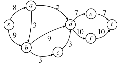
(a) A flow network with source $s$ and sink $t$.

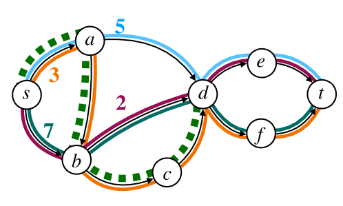
(b) An MFD into 4 paths of weights 5,3,7,2, respectively. The green dashed path is a subpath of the orange path.

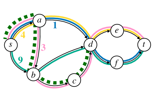
(c) An MFD into 4 paths of weights 3,4,1,9, respectively. The green dashed path is a subpath of the pink path.

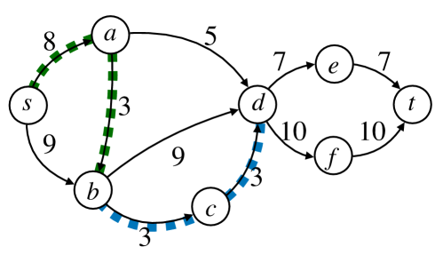
(d) The two subpaths (red and blue) of the green dashed path that are maximal safe paths for all FDs.

Figure 1: Flow decompositions and safe paths. The flow network in 1(a) admits different MFDs, in 1(b) and in 1(c). The path $(s,a,b,c,d)$ (dashed green) is a maximal safe path for MFDs, i.e., it is a subpath of some path of all MFDs and it cannot be extended without losing this property. However, the path $(s,a,b,c,d)$ is not safe for all FDs. Indeed, its two subpaths $(s,a,b)$ (dashed red in 1(d)) and $(b,c,d)$ (dashed blue in 1(d)) are maximal safe paths for all FDs. To see this, note that the excess flow of $(s,a,b)$ is 3, while the excess flow of $(s,a,b,c)$ (and of $(s,a,b,c,d)$) is $-6$.

For concreteness, we now describe the ILP models from [15] for finding a flow decomposition into $k$ weighted paths in a DAG. They consist of (i) modeling the $k$ paths via the $x_{uvi}$ variables (with constraints (1)), (ii) adding path-weight variables $w_{1},\dots,w_{k}$, and (iii) requiring that these weighted paths form a flow decomposition, via the following (non-linear) constraint:

$$\sum_{i\in\{1,\dots,k\}}x_{uvi}w_{i}=f_{uv}, \forall(u,v)\in E.$$ (3)

This constraint can then be easily linearized by introducing additional variables and constraints; see e.g. [15] for these technical details. However, as mentioned above, the precise formulation of the ILP model $\mathcal{M}$ for a problem is immaterial for our method. Only the two assumptions on $\mathcal{M}$ made above matter for obtaining our results.

Safety.

Given a problem on a graph $G$ whose solutions consist of $k$ paths in $G$, we say that a path $P$ is safe if for any solution $P_{1},\dots,P_{k}$ to the problem, there exists some $i\in\{1,\dots,k\}$ such that $P$ is a subpath of $P_{i}$. If the problem is given as an ILP model $\mathcal{M}$, we also say that $P$ is safe for $\mathcal{M}$. We say that $P$ is a maximal safe path, if $P$ is a safe path and there is no larger safe path containing $P$ as subpath. [27] characterized safe paths for all FDs (not necessarily of minimum size) using the excess flow $f_{P}$ of a path $P$, defined as the flow on the first edge of $P$ minus the flow on the edges out-going from the internal nodes of $P$, and different from the edges of $P$ (see Figure 1(d) for an example). It holds that $P$ is safe for all FDs if and only if $f_{P}>0$ [27]. The excess flow can be computed in time linear in the length of $P$ (assuming we have pre-computed the flow outgoing from every node), giving thus a linear-time verification of whether $P$ is safe.

A basic property of safe solutions is that any sub-solution of them is also safe. Computing safe paths for MFDs can thus potentially lead to joining several safe paths for FDs, obtaining longer paths from the unknown sequences we are trying to assemble. See Figure 1 for an example of a maximal safe path for MFDs and two maximal subpaths of it that are safe for FDs.

2.2 Finding Maximal Safe Paths for MFD via ILP

We now present a method for finding all maximal safe paths for MFD via ILP. The basic idea is to define an inner “safety test” which can be repeatedly called as part of an outer algorithm over the entire instance to find all maximal safe paths. Because calls to the ILP solver are expensive, the guiding choice for our overall approach is to minimize the number of ILP calls. This inspires us to test the safety of a group of paths as the inner safety test, which we achieve by augmenting our ILP model so that it can give us information about the safety of the paths in the set. We use this to define a recursive algorithm to fully determine the safety status of each path in a group of paths. We can then structure the safety test in either a top-down manner (starting with long unsafe paths and shrinking them until they are safe) or a bottom-up manner (starting with short safe paths and lengthening them until they become unsafe).

2.2.1 Safety test (inner algorithm)

Let $\mathcal{M}(\mathcal{V},\mathcal{C})$ be an ILP model as discussed in Section 2.1; namely, its $k$ solution paths are modeled by binary variables $x_{uvi}$ for each $(u,v)\in E$ and each $i\in\{1,\dots,k\}$. We assume that $\mathcal{M}(\mathcal{V},\mathcal{C})$ is feasible (i.e., the problem admits at least one solution). We first show how to modify the ILP model so that, for a given set of paths, it can tell us one of the following: (1) a set of paths that are not safe (the remaining being of unknown status), or (2) that all paths are safe. The idea is to maximize the number of paths that can be simultaneously avoided from the given set of paths.

Let $\mathcal{P}$ be a set of paths. For each path $P\in\mathcal{P}$, we create an auxiliary binary variable $\gamma_{P}$ that indicates:

$$\gamma_{P}\equiv\begin{cases}1&\text{if $P$ was avoided in the solution},\\ 0&\text{otherwise}.\end{cases}$$ (4)

Since the model solutions are paths (i.e., not repeating nodes), we can encode whether $P$ appears in the solution by whether all of the $\ell-1$ edges of $P$ appear simultaneously. Using this fact, we add a new set of constraints $\mathcal{R}(\mathcal{P})$ that include the $\gamma_{P}$ indicator variables for each path $P\in\mathcal{P}$:

$$\mathcal{R}(\mathcal{P}):=\{x_{v_{1}v_{2}i}+x_{v_{2}v_{3}i}+\cdots+x_{v_{\ell-1}v_{\ell}i}$$

$$\quad\leq\ell-1-\gamma_{P}:\forall i\in\{1,\dots,k\},\forall P\in\mathcal{P}\}.$$ (5)

Next, as the objective function of the ILP model, we require that it should maximize the number of avoided paths from $\mathcal{P}$, i,e., the sum of the $\gamma_{P}$ variables:

$$\max\sum_{P\in\mathcal{P}}\gamma_{P}.$$ (6)

All paths $P$ such that $\gamma_{P}=1$ are unsafe, since they were avoided in some minimum flow decomposition. Conversely, if the objective value of Eq. 6 was $0$, then $\gamma_{P}=0$ for all paths in $\mathcal{P}$, and it must be that all paths in $\mathcal{P}$ are safe (if not, at least one path could be avoided and increase the objective). We encapsulate this group testing ILP in a function GroupTest$(\mathcal{M},\mathcal{P})$ that returns a set $\mathcal{N}\subseteq\mathcal{P}$ with the properties that: (1) if $\mathcal{N}=\emptyset$, then all paths in $\mathcal{P}$ are safe, and (2) if $\mathcal{N}\neq\emptyset$, then all paths in $\mathcal{N}$ are unsafe (and $|\mathcal{N}|$ is maximized).

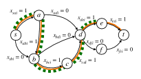
Figure 2: Illustration of modeling a solution path and a tested path via binary edge variables and safety verification constraints. The $i$^th solution path $P_{i}$ is shown in orange, and a tested path $P$ is shown in dashed green. Constraint (2.2.1) includes $x_{sai}+x_{abi}+x_{bci}+x_{cdi}+x_{dei}\leq 5-\gamma_{P}$. This simplifies to $\gamma_{P}\leq 0$, thus forcing $\gamma_{P}=0$, which indicates $P$ was not avoided in the solution.

We employ GroupTest$(\mathcal{M},\mathcal{P})$ to construct a recursive procedure GetSafe$(\mathcal{M},\mathcal{P})$ that determines all safe paths in $\mathcal{P}$, as shown in Algorithm 1.

Input: A feasible ILP model $\mathcal{M}(\mathcal{V},\mathcal{C})$, and a set of paths $\mathcal{P}$

Output: Those paths $P\in\mathcal{P}$ that are safe for $\mathcal{M}(\mathcal{V},\mathcal{C})$

1

2 Procedure GetSafe$(\mathcal{M},\mathcal{P})$

3       $\mathcal{N}$ = GroupTest$(\mathcal{M},\mathcal{P})$ if $\mathcal{N}=\emptyset$ then

4             return $\mathcal{P}$ 

5      else

6             return GetSafe$(\mathcal{M},\mathcal{P}\setminus\mathcal{N})$ 

7      

Algorithm 1 Testing a set of paths $\mathcal{P}$ for safety.

We note that in the special case that $|\mathcal{P}|=1$, GetSafe$(\mathcal{M},\mathcal{P})$ makes only a single call to the ILP via GroupTest$(\mathcal{M},\mathcal{P})$ to determine whether not the given path is safe. With this safety test for a single path, we can easily adapt a standard two-pointer approach as the outer algorithm to find all maximal safe paths for MFD by starting with some MFD solution $P_{1},\dots,P_{k}$ of $\mathcal{M}(\mathcal{V},\mathcal{C})$. This same procedure was used in [26] to find all maximal safe paths for FD, using an excess flow check as the inner safety algorithm.

2.2.2 Find all maximal safe paths (outer algorithm)

We give two algorithms for finding all maximal safe paths. Both algorithms use a similar approach, however the first uses a top-down approach starting from the original full solution paths and reports all safe paths (these again must be maximal safe), and then trims all the unsafe paths to find new maximal safe paths. The second is bottom-up in that it tries to extend known safe subpaths until they cannot be further extended (and at this point must be maximal safe). We present the first algorithm in detail and defer discussion of the second to the appendix.

We say a set of subpaths $\mathcal{T}=\{P_{i}[l_{i},r_{i}]\}$ is a trimming core provided that for any unreported maximal safe path $P=P_{i}[l,r]$, there is a $P_{i}[l_{i},r_{i}]\in\mathcal{T}$, where $l_{i}\leq l\leq r\leq r_{i}$.

Input: An ILP model $\mathcal{M}$ and a trimming core set $\mathcal{T}$

Output: All maximal safe paths for $\mathcal{M}$ that are trimmed subpaths of $\mathcal{T}$

1

2 Procedure AllMaxSafe-TopDown$(\mathcal{M},\mathcal{T}$)

3       $\mathcal{S}$ = GetSafe$(\mathcal{M},\mathcal{T})$ for $P_{i}[l_{i},r_{i}]\in\mathcal{S}$ do

4             output $P_{i}[l_{i},r_{i}]$ 

5      $\mathcal{U}=\mathcal{T}\setminus\mathcal{S}$ $\mathcal{L}=\{P_{i}[l_{i}+1,r_{i}]:P_{i}[l_{i},r_{i}]\in\mathcal{U},(r_{i}=|P_{i}|\ \textnormal{{or}}\ P_{i}[l_{i}+1,r_{i}+1]\in\mathcal{U})\}$ $\mathcal{R}=\{P_{i}[l_{i},r_{i}-1]:P_{i}[l_{i},r_{i}]\in\mathcal{U},(l_{i}=1\ \textnormal{{or}}\ P_{i}[l_{i}-1,r_{i}-1]\in\mathcal{U})\}$ $\mathcal{P}=\mathcal{L}\cup\mathcal{R}$ if $\mathcal{P}\neq\emptyset$ then

6             AllMaxSafe-TopDown$(\mathcal{M},\mathcal{P})$ 

7      

8

Algorithm 2 An algorithm to compute all maximal safe paths that can be trimmed from a trimming core set $\mathcal{T}$.

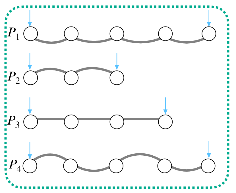
(a) First group test

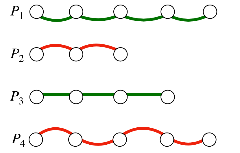
(b) Result: $\{P_{1},P_{3}\}$ are safe, $\{P_{2},P_{4}\}$ are unsafe

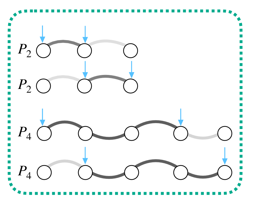
(c) Second group test

Figure 3: Illustration of the initial group tests performed by Algorithm 2. Fig. 3(a) shows the first group test (using Algorithm 1) on MFD solution paths $\{P_{1},P_{2},P_{3},P_{4}\}$; suppose $\{P_{1},P_{3}\}$ were safe (Fig. 3(b)); these are then reported as maximal safe. In this case we trim $\{P_{2},P_{4}\}$ on both the left and right and make the next group test shown in Fig. 3(c).

We will use the original $k$ solution paths $\{P_{i}\}$ as our initial trimming core; the complete algorithm is given in Algorithm 2. See Fig. 3 in the appendix for an illustration of the algorithm’s initial steps. The algorithm first checks if any of the paths in $\mathcal{T}$ are safe; if so, these are reported as maximal safe. For those paths that were unsafe, it then considers trimming one vertex from the left and one vertex from the right to create new subpaths. Of these subpaths, some may be contained in a safe path in $\mathcal{T}$; these subpaths can be ignored as they are not maximal safe. The algorithm recurses on those subpaths whose safety status cannot be determined (lines $6$–$10$). In this way, the algorithm maintains the invariant that no paths in $\mathcal{T}$ are properly contained in a safe path; thus paths reported in line $4$ must be maximal safe.

3 Experiments

To test the performance of our methods, we computed safe paths using different safety approaches and reported the quality and running time performances as described below. Additional details on the experimental setup are given in the appendix.

Implementation details – SafeMFD.

We implemented the previously described algorithms to compute all maximal safe paths for minimum flow decompositions in Python. The implementation, SafeMFD, uses the package NetworkX [20] for graph processing and the package gurobipy [19] to model and solve the ILPs and it is openly available. Our fastest variant (see Table 2 in the appendix for a comparison of running times) implements Algorithm 2 using the group testing in Algorithm 1. We used this variant to compare against other safety approaches. All tested variants of SafeMFD implement the following two optimizations:

1. Before processing an input flow graph we contract it using Y-to-V contraction [51], which is known [30] to maintain (M)FD solution paths. Moreover, since edges in the contracted graph correspond to extended unitigs [35, 24, 29], source-to-sink edges are further removed from the contracted graph and reported as safe. As such, our algorithms compute all maximal safe paths for funnels [17, 26] without using the ILP.

2. Before testing the safety of a path we check if its excess-flow [26] is positive. If this is the case, the path is removed from the corresponding test. Having positive excess flow implies safety for all flow decomposition and thus also safety for minimum flow decompositions.

Safety approaches tested.

We compare the following state-of-the-art safety approaches:

EUnitigs: 

Maximal paths made up of a prefix of nodes with in-degree one followed by nodes with out-degree one; also called extended unitigs [51, 35, 24, 29]. We use the C++ implementation provided by Khan et al. [26] (which computes only the extended unitigs contained in FD paths).

SafeFlow: 

Maximal safe paths for all flow decompositions [26]. We use the C++ implementation provided by Khan et al. [26].

SafeMFD: 

Maximal safe paths for all minimum flow decompositions, as proposed in this work. Every flow graph processed is given a time budget of 2 minutes. If a flow graph consumes its time budget, the solution of SafeFlow is output instead.

SafeEPC: 

Maximal safe paths for all constrained path covers of edges. Previous authors [8, 26] have considered safe path covers of the nodes, but for a more fair comparison, we instead use path covers of edges. To this end, we transform the input graphs by splitting every edge by adding a node in the middle and run the C++ implementation provided by the authors of [8]. Since flow decompositions are path covers of edges, safe paths for all edge path covers are subpaths of safe paths for MFD. However, we restrict the path covers to those of minimum size and minimum size plus one, as recommended by the authors of [8] to obtain good coverage results while maintaining high precision.

All safety approaches require a post processing step for removing duplicates, prefixes and suffixes. We use the C++ implementation provided by [26] for this purpose.

Datasets.

We use two datasets of flow graphs inspired by RNA transcript assembly. The datasets were created by simulating abundances on a set of transcripts and then perfectly superposing them into a splice graphs that are guaranteed to respect flow conservation. As such, the ground truth corresponds to a flow decomposition (not necessarily minimum). To avoid a skewed picture of our results we filtered out trivial instances with a unique flow decomposition (or funnels, see [17, 26]) from the two datasets.

Catfish: 

Created by [48], it includes 100 simulated human, mouse and zebrafish transcriptomes using Flux-Simulator [18] as well as 1,000 experiments from the Sequence Read Archive simulating abundances using Salmon [40]. We took one experiment per dataset, which corresponds to 27,696 non-trivial flow graphs.

RefSim: 

Created by [8] from the Ensembl [57] annotated transcripts of GRCh.104 homo sapiens reference genome, and later augmented by Khan et al. [26] with simulated abundances using the RNASeqReadSimulator [32]. This dataset has 10,323 non-trivial graphs.

Quality metrics.

We use the same quality metrics employed by previous multi-assembly safety approaches [8, 26]. We provide a high-level description of them for completeness.

Weighted precision of reported paths: 

As opposed to normal precision, the weighted version considers the length of the reported subpaths. It is computed as the total length of the correctly reported subpaths divided by the total length of all reported subpaths. A reported subpath is considered correct if and only if it is a subpath of some path in the ground truth (exact alignment of exons/nodes).

Maximum coverage of a ground truth path $P$: 

The longest segment of $P$ covered by some reported subpath (exact alignment of exons/nodes), divided by $|P|$.

We compute the weighted precision of a graph as the average weighted precision over all reported paths in the graph, and the maximum coverage of a graph as the average maximum coverage over all ground truth paths in the graph.

F-Score of a graph: 

Harmonic mean between weighted precision and maximum coverage of a graph, which assigns a global score to the corresponding approach on the graph.

These metrics are computed per flow graph and reported as an average. In the case of the Catfish dataset the metrics are computed in terms of exons (nodes), since genomic coordinates of exons are missing, whereas in the case of the RefSim dataset the metrics are computed in terms of genomic positions, as this information is present in the input.

4 Results and Discussion

Table 1: Summary of quality metrics for both datasets. For Catfish, the metrics are computed in terms of nodes/exons and for RefSim in terms of genomic positions; $t$ is the number of ground truth paths.

Dataset	Graphs	Algorithm	Max. Coverage	Wt. Precision	F-Score
Catfish	All (100%)	EUnitigs	0.60	1.00	0.74
		SafeEPC	0.60	0.99	0.74
		SafeFlow	0.71	1.00	0.82
		SafeMFD	0.88	0.99	0.93
RefSim	$t\leq 10$ (68%)	EUnitigs	0.72	1.00	0.83
		SafeEPC	0.73	1.00	0.84
		SafeFlow	0.84	1.00	0.91
		SafeMFD	0.97	0.99	0.98
	$t\leq 15$ (84%)	EUnitigs	0.70	1.00	0.82
		SafeEPC	0.71	1.00	0.83
		SafeFlow	0.83	1.00	0.90
		SafeMFD	0.96	0.98	0.97
	All (100%)	EUnitigs	0.68	1.00	0.80
		SafeEPC	0.69	0.99	0.81
		SafeFlow	0.81	1.00	0.89
		SafeMFD	0.93	0.91	0.90

In the Catfish dataset, EUnitigs and SafeFlow ran in less than a second, while SafeEPC took approximately 30 seconds to compute. On the other hand, solving a harder problem, SafeMFD took approximately 1.5 hours to compute in the rest of the dataset, timing out in only 54 graphs (we use a cutoff of 2 minutes), i.e., only 0.2% of the entire dataset. This equates to only 0.2 seconds on average per solved graph, underlying the scalability of our approach.

Table 1 shows that SafeMFD, on average, covers close to 90% of the ground truth paths, while maintaining a high precision (99%). This corresponds to an increase of approximately 25% in coverage against its closest competitor SafeFlow. SafeMFD also dominates in the combined metric of F-Score, being the only safe approach with F-Score over 90%. Figure 4 in the appendix shows the metrics on graphs grouped by number $t$ of ground truth paths, indicating the dominance in coverage and F-Score of SafeMFD across all values of $t$, and indicating that the decrease in precision appears for large values of $t$ ($t\geq 12$).

In the harder RefSim dataset, EUnitigs and SafeFlow also ran in less than a second, while SafeEPC took approximately 2 minutes. In this case, SafeMFD ran out of time in 1,562 graphs (15% of the entire dataset); however, recall that in these experiments we allow a time budget of only 2 minutes. In the rest of the dataset, it took approximately 7.5 hours in total, corresponding to only 3 seconds on average per graph, again underlying that our method, even though it solves many NP-hard problems for each input graph, overall scales sufficiently well.

Table 1 shows that again SafeMFD dominates in coverage, being the only approach obtaining coverage over 90%, with is a 15% improvement over SafeFlow. This time its precision drops to close to 90%, and obtaining an F-Score of 90%, very similar to its closest competitor, SafeFlow. However, recall that coverage is computed only from correctly aligned paths, thus the drop in precision comes only from safe paths not counting in the coverage metric. If we restrict the metrics to graphs with at most 15 ground truth paths, which is still a significant proportion (84%) of the entire dataset, then SafeMFD has a very high precision (98%) while improving coverage by 15% with respect to SafeFlow. Thus, the drop in precision occurs in graphs with a large number of ground truth paths, which can also be corroborated by Figure 5 in the appendix.

These drops in precision (both in RefSim and Catfish) for large $t$ can be explained by the fact that a larger number of ground truth paths produces more complex splice graphs and introduces more artificial solutions of potentially smaller size. As such, the larger $t$, the less likely that the ground truth is a minimum flow decomposition of the graph, and thus the more likely that SafeMFD reports incorrect solutions. This motivates future work on safety not only on minimum flow decompositions but also in flow decompositions of at most a certain size, analogously to how it is done for SafeEPC. This is still easily achievable with our framework by just changing the ILP blackbox, and keeping everything else unchanged (e.g., the inner and outer algorithms). Namely, instead of formulating the ILP model $\mathcal{M}(\mathcal{V},\mathcal{C})$ to admit solutions of exactly optimal $k$ paths, it can be changed to allow solutions of at most some $k^{\prime}$ paths, with $k^{\prime}$ greater than the optimal $k$. If $k^{\prime}$ is also greater than the number of ground truth paths in these complex graphs, then safe paths are fully correct, meaning that we overall increase precision.

5 Conclusion

RNA assembly is a difficult problem in practice, with even the top tools reporting low precision values. While there are still many issues that can introduce uncertainty in practice, we can now provide a major source of additional information during the process: which RNA fragments must be included in any parsimonious explanation of the data? Though others have considered RNA assembly in the safety framework [58, 26], we are the first to show that safety can be practically used even when we look for optimal (i.e., minimum) size solutions. Our experimental results show that safe paths for MFD clearly outperform other safe approaches for the Catfish dataset, commonly used in this field. On a significant proportion of the second dataset, safe paths for MFD still significantly outperforms other safe methods.

More generally, this is the first work to show that the safety framework can be practically applied to NP-hard problems, where the inner algorithm is an efficient test of safety of a group of paths, and the outer algorithm guides the applications of this test. Because our method was very successful on our test data set, there is strong motivation to try the approach to on other NP-hard graph problems whose solutions are sets of paths. For example, we could study other variations on MFD, such as finding flow decompositions minimizing the longest path (NP-hard when flow values are integer [4, 43]). The approach given in this paper can also be directly extended to find decompositions into both cycles and paths [16], though not trails and walks, because they repeat edges. We could also formulate a safety test for classic NP-hard graph problems like Hamiltonian path.

Acknowledgements

This work was partially funded by the European Research Council (ERC) under the European Union’s Horizon 2020 research and innovation programme (grant agreement No. 851093, SAFEBIO), partially by the Academy of Finland (grants No. 322595, 352821, 346968), and partially by the US National Science Foundation (NSF) (grants No. 1759522, 1920954).

Appendix 0.A Additional Figures

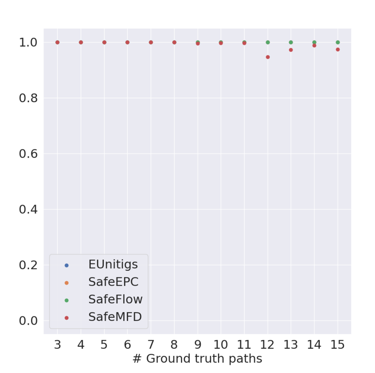
(a) Weighted Precision

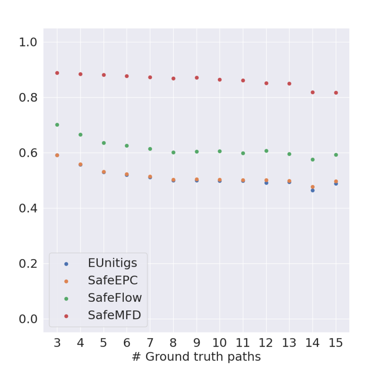
(b) Maximum Coverage

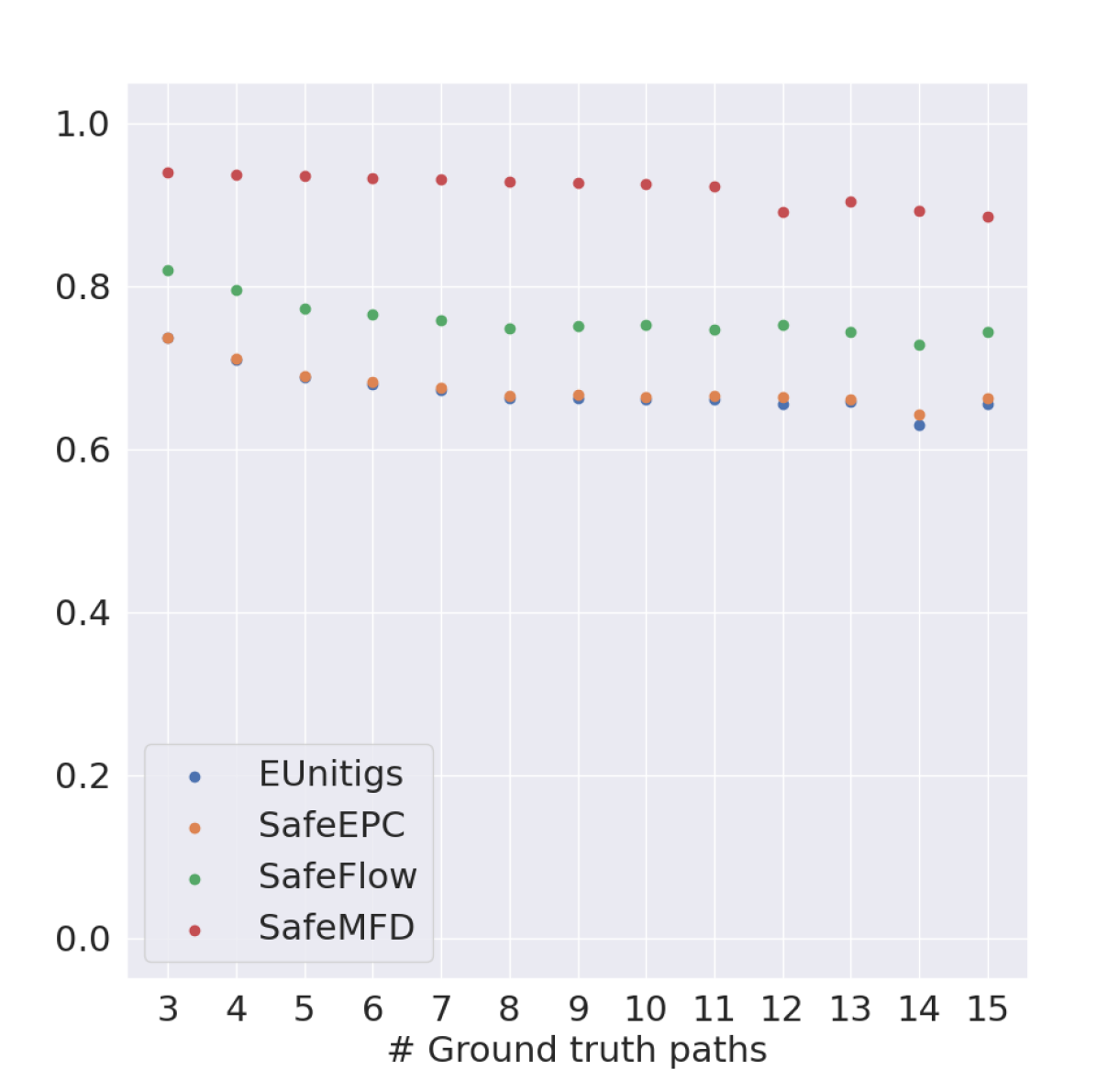
(c) F-Score

Figure 4: Quality metrics on graphs distributed by number of paths in the ground truth for the Catfish dataset. The metrics are computed in terms of exons/nodes.

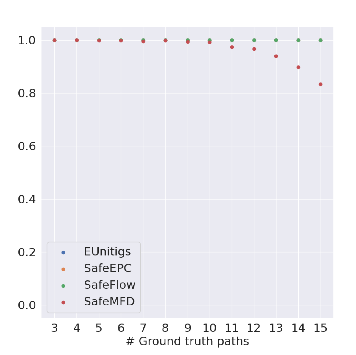
(a) Weighted Precision

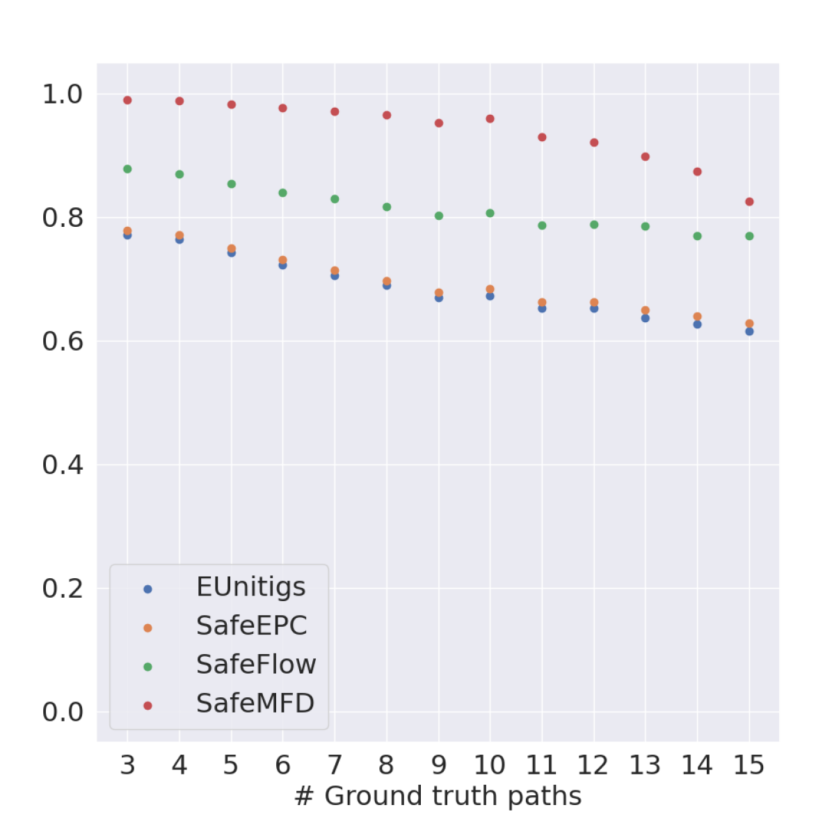
(b) Maximum Coverage

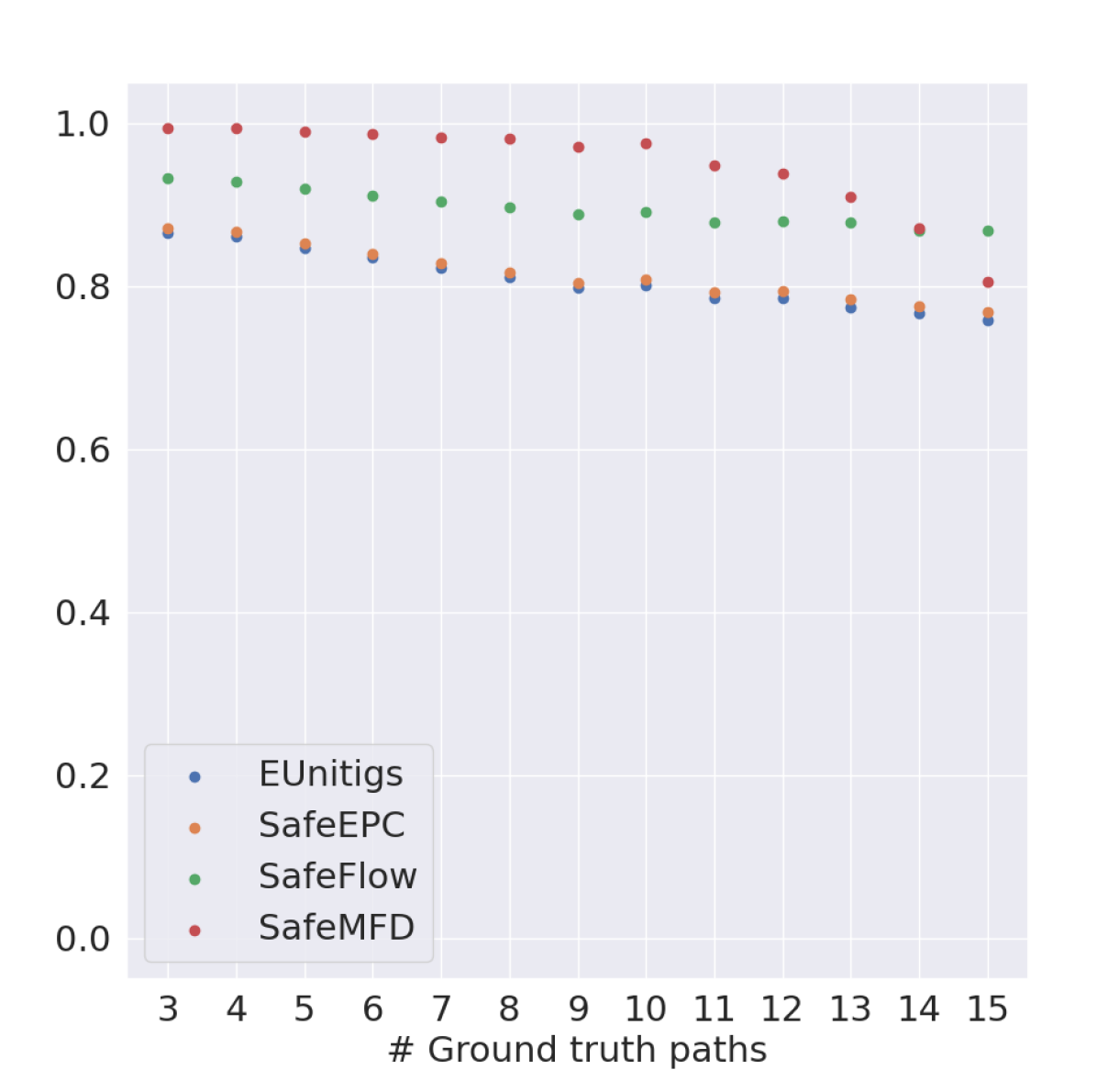
(c) F-Score

Figure 5: Quality metrics on graphs distributed by number of paths in the ground truth for the RefSim dataset. The metrics are computed in terms of genomic positions.

Appendix 0.B Additional Algorithms and Experimental Results

0.B.1 The bottom-up algorithm

Algorithm 3, detailed below, uses a bottom-up group-testing strategy to find all maximal safe paths.

Definition 1

We say a set of subpaths $\mathcal{E}=\{P_{i}[l_{i},r_{i}]\}$ is an extending core provided all paths in $\mathcal{E}$ are safe and for any unreported maximal safe path $P=P_{i}[l,r]$, there is a $P_{i}[l_{i},r_{i}]\in\mathcal{E}$, where $l\leq l_{i}\leq r_{i}\leq r$.

Note that maximal FD-safe subpaths provide an extending core (as well just the set of all single-edge subpaths in each path). Algorithm 3 provides an algorithm to find all maximal safe paths based on group testing, starting from an extending core. The idea is to try both left-extending (by one) and right-extending (by one) each subpath in the core; if neither of these extensions are safe, then we know that that core subpath must be maximal safe. Testing all extensions can done quickly using Algorithm 1. We then recurse on a new core set consisting of those extensions that were found to be safe.

Input: An ILP model $\mathcal{M}$ and an extending core set $\mathcal{E}$

Output: All maximal safe paths for $\mathcal{M}$ that extend some path from $\mathcal{E}$

1

2 Procedure AllMaxSafe-BottomUp$(\mathcal{M},\mathcal{E})$

3       $\mathcal{L}=\{P_{i}[l_{i}-1,r_{i}]:P_{i}[l_{i},r_{i}]\in\mathcal{E},l_{i}>1\}$ $\mathcal{R}=\{P_{i}[l_{i},r_{i}+1]:P_{i}[l_{i},r_{i}]\in\mathcal{E},r_{i}<|P_{i}|\}$ $\mathcal{P}=\mathcal{L}\cup\mathcal{R}$ $\mathcal{S}$ = GetSafe$(\mathcal{M},\mathcal{P})$ for $P_{i}[l_{i},r_{i}]\in\mathcal{E}$ do

4             if $P_{i}[l_{i}-1,r_{i}]\notin\mathcal{S}$ and $P_{i}[l_{i},r_{i}+1]\notin\mathcal{S}$ then

5                   output $P_{i}[l_{i},r_{i}]$ 

6            

7      if $\mathcal{S}\neq\emptyset$ then

8             AllMaxSafe-BottomUp$(\mathcal{M},\mathcal{S})$ 

9      

10

Algorithm 3 An algorithm to output all maximal safe subpaths that can be extended from an extending core set $\mathcal{E}$.

0.B.2 The two-pointer algorithm

As we observed in Section 2.2.1, we can test whether a single path $P$ is safe using one ILP call. We will assume that this test is encapsulated as a procedure IsSafe$(\mathcal{M},P)$. Once we can test whether a single path is safe for $\mathcal{M}(\mathcal{V},\mathcal{C})$, we can adopt a standard approach to compute all maximal safe paths. Namely, we start by computing one solution of $\mathcal{M}(\mathcal{V},\mathcal{C})$, $P_{1},\dots,P_{k}$ and then compute maximal safe paths by a two-pointer technique that for each path $P_{i}$, finds all maximal safe paths by just a linear number of calls to the procedure IsSafe [26].

This works as follows. We use two pointers, a left pointer $L$, and a right pointer $R$. Initially, $L$ points to the first node of path $P_{i}$ and $R$ to the second node. As long as the subpath of $P_{i}$ between $L$ and $R$ is safe, we move the right pointer to the next node on $P_{i}$. When this subpath is not safe, we output the subpath between $L$ and the previous location of $R$ as a maximal safe path, and we start moving the left pointer to the next node on $P_{i}$, until the subpath between $L$ and $R$ is safe. We stop the procedure once we reach the end of $P_{i}$. We summarize this procedure as Algorithm 4; see also Figure 6 for an example.

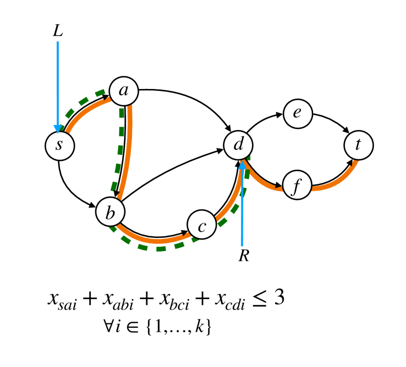
(a) Current iteration

(b) Right pointer movement

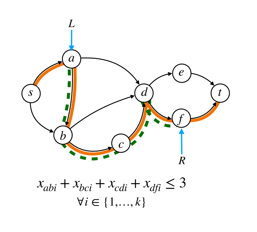
(c) Left pointer movement

Figure 6: Illustration of the two-pointer algorithm applied on a flow decomposition path $P_{i}$ (in orange). In each sub-figure, the subpath $P$ (dashed green) between the nodes pointed by the left pointer $L$ and the right pointer $R$ is tested for safety, by adding constraints $\mathcal{S}(P)$. In 6(a), IsSafe$(\mathcal{M},P)$ returns True, and the right pointer advances on $P_{i}$. In 6(b), IsSafe$(\mathcal{M},P)$ returns False, and the previous subpath from 6(a) is output as a maximal safe path. In 6(c), the left pointer has advanced, and the new path $P$ is tested for safety.

Input: An ILP model $\mathcal{M}$ and one of its $k$ solution paths, $P_{i}=(v_{1},\dots,v_{t})$, $t\geq 2$

Output: All maximal safe subpaths of $P_{i}$ for $\mathcal{M}$

1 Procedure AllMaxSafe-TwoPointer$(\mathcal{M},P_{i})$

2       $L\leftarrow 1$, $R\leftarrow 2$ while True do

3             while IsSafe$(\mathcal{M},P_{i}[L,R])$ and $R\leq t$ do

4                   $R\leftarrow R+1$ 

5            output $P_{i}[L,R-1]$ if $R>t$ then  return ;

6             while not IsSafe$(\mathcal{M},P_{i}[L,R])$ do

7                   $L\leftarrow L+1$ 

8            

9      

10

Algorithm 4 The two-pointer algorithm applied to compute all maximal subpaths of a given solution path $P_{i}$

0.B.3 Running time experiments among different variants proposed

We conducted the experiments on an isolated Linux server with AMD Ryzen Threadripper PRO 3975WX CPU with 32 cores (64 virtual) and 504GB of RAM. Time and peak memory usage of each program were measured with the GNU time command. SafeMFD was allowed to run Gurobi with 12 threads. All C++ implementations were compiled with optimization level 3 (-O3 flag). Running time and peak memory is computed and reported per dataset.

SafeMFD includes the following four variants computing maximal safe paths:

TopDown

: Implements Algorithm 2 using the group testing in Algorithm 1.

BottomUp

: Implements Algorithm 3 (Section 0.B.1) using the group testing in Algorithm 1.

TwoPointer

: Implements Algorithm 4 (Section 0.B.2), the traditional two-pointer algorithm [26].

TwoPointerBin

: Same as previous variant, but it additionally replaces the linear scan employed to extend and reduce the currently processed safe path by a binary search.

To compare between our four different variants we first run them all on every dataset, and then filter out those graphs that ran out of time in some variant. This way we ensure that no variant consumes its time budget and thus our running time measurements are not skewed by the unsuccessful inputs’ timeouts. Applying this filter we removed 83 graphs from the Catfish dataset (0.3%) and 4,515 graphs from the RefSim dataset (43.74%).

Dataset (# Graphs)	Variant	Time (hh:mm:ss)	# ILP calls
Catfish (27,613)	TopDown	01:13:27	124,676
	BottomUp	03:22:13	212,774
	TwoPointer	04:21:44	226,365
	TwoPointerBin	03:31:57	216,540
RefSim (5,808)	TopDown	04:38:41	55,450
	BottomUp	11:55:20	76,837
	TwoPointer	13:48:00	127,352
	TwoPointerBin	11:34:02	119,218

Table 2: Running times and number of ILP calls in four different variants of SafeMFD.

Table 2 shows the running times and number of ILP calls of the different variants on both datasets. TopDown clearly outperforms the rest, being at least twice as fast, and performing (roughly) half many ILP calls. While BottomUp is analogous to TopDown, the superiority of the latter can be explained by the length maximal safe paths. Since maximal safe paths are long it is faster to obtain them by reducing unsafe paths (TopDown) than by extending safe paths (BottomUp and both TwoPointer variants). On the other hand, TwoPointer is the slowest variant and BottomUp and TwoPointerBin obtain similar improvements (over TwoPointer) by following different strategies. While BottomUp reduces the number of ILP calls more than TwoPointerBin (better appreciated in the RefSim dataset), the ILP calls of BottomUp take longer (since BottomUp tests several paths at the same time and TwoPointerBin only one), and thus the total running times of both is similar. This motivates future work on combining both approaches, while processing the paths starting from unsafe (as in TopDown) for better performance.

Appendix 0.C Hardness of Testing MFD Safety

In this section we give a Turing-reduction from the UNIQUE 3SAT problem (U3SAT) to the problem of determining if a given path $P$ in a flow network $G$ is safe for minimum flow decomposition (call this problem MFD-SAFETY). A 3SAT instance belongs to U3SAT if and only if it has exactly one satisfying assignment. U3SAT has been shown to be NP-hard under randomized reductions [52], but it is open as to whether it is NP-hard in general.

The reduction leverages the construction in [22] that reduces 3SAT to minimum flow decomposition. We first briefly review this construction: A variable gadget (see Fig. 4 in [22]) is created for each 3SAT variable $x$ and a clause gadget (see Fig. 5 in [22]) is created for each 3SAT clause. Positive literals in each clause receive flow from the left side of the corresponding variable gadget, whereas negative literals receive flow from the right side. Theorem VI.1 in [22] establishes that a 3SAT instance is satisfiable if and only if the constructed flow network has a minimum flow decomposition of a certain size. Any flow decomposition achieving this size must have a specific structure; in particular, there must be a flow path of weight $4$ that either travels up the left side of the gadget (setting $x$ to TRUE), or the right side (setting $x$ to FALSE).

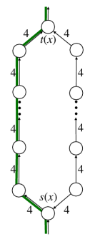
Figure 7: The variable gadget from [22], showing only the weight $4$ edges (other edges have weights from $\{1,2\})$. A key property established in [22] is that if the 3SAT instance is satisfiable then in a minimum flow decomposition, a weight $4$ flow path must travel up either the left side of the gadget (as shown), or the right side. A left flow path indicates the variable should be set to TRUE, while right indicates FALSE. We leverage this construction to reduce U3SAT to MFD-SAFETY.

Theorem 0.C.1

There is a polynomial time Turing-reduction from U3SAT to MFD-SAFETY.

Proof

To obtain the desired Turing-reduction algorithm, instead of checking the size of the MFD, we will instead sequentially check the MFD-SAFETY of the aforementioned side paths traveling up the left and right sides of each variable gadget. Provided each variable gadget has exactly one safe side path we can then check the corresponding truth assignment to see if each clause is satisfied. If yes, we accept the instance as belonging to U3SAT, otherwise we reject.

Suppose the instance does belong to U3SAT. In this case there is a satisfying assignment so the MFD must have the structure as described above. Furthermore, since there is exactly one satisfying assignment, exactly one side path of each variable gadget must be safe and so our algorithm finds it and then verifies that the truth assignment satisfies each clause, thus accepting the instance. On the other hand, if the instance does not belong to U3SAT it could either be unsatisfiable or have multiple satisfying assignments. If unsatisfiable, no matter whether the safety checks pass, the corresponding assignment will not satisfy all clauses, so the instance will be rejected. If there are multiple solutions, then any variable that can be both TRUE and FALSE will not have a safe side path in the MFD. This means the safety check will fail and the instance will again be rejected. ∎

References

- [1] Ravindra K Ahuja, Thomas L Magnanti, and James B Orlin. Network flows. Cambridge, Mass.: Alfred P. Sloan School of Management, Massachusetts, 1988.
- [2] Jasmijn A Baaijens, Leen Stougie, and Alexander Schönhuth. Strain-aware assembly of genomes from mixed samples using flow variation graphs. In International Conference on Research in Computational Molecular Biology, pp. 221–222. Springer, 2020.
- [3] Jasmijn A Baaijens, Bastiaan Van der Roest, Johannes Köster, Leen Stougie, and Alexander Schönhuth. Full-length de novo viral quasispecies assembly through variation graph construction. Bioinformatics, 35(24):5086–5094, 2019.
- [4] Georg Baier. Flows with path restrictions. Cuvillier Verlag, 2004.
- [5] Elsa Bernard, Laurent Jacob, Julien Mairal, and Jean-Philippe Vert. Efficient RNA isoform identification and quantification from RNA-Seq data with network flows. Bioinformatics, 30(17):2447–2455, 2014.
- [6] V. Bonnici, G. Franco, and V. Manca. Spectral concepts in genome informational analysis. Theoretical Computer Science, 894:23–30, 2021. Building Bridges – Honoring Nataša Jonoska on the Occasion of Her 60th Birthday.
- [7] Manuel Cáceres, Massimo Cairo, Andreas Grigorjew, Shahbaz Khan, Brendan Mumey, Romeo Rizzi, Alexandru I. Tomescu, and Lucia Williams. Width helps and hinders splitting flows. In Shiri Chechik, Gonzalo Navarro, Eva Rotenberg, and Grzegorz Herman, editors, 30th Annual European Symposium on Algorithms, ESA 2022, September 5-9, 2022, Berlin/Potsdam, Germany, volume 244 of LIPIcs, pp. 31:1–31:14. Schloss Dagstuhl - Leibniz-Zentrum für Informatik, 2022.
- [8] Manuel Cáceres, Brendan Mumey, Edin Husić, Romeo Rizzi, Massimo Cairo, Kristoffer Sahlin, and Alexandru I. Tomescu. Safety in multi-assembly via paths appearing in all path covers of a dag. IEEE/ACM Transactions on Computational Biology and Bioinformatics, 2022. Accepted.
- [9] Massimo Cairo, Shahbaz Khan, Romeo Rizzi, Sebastian S. Schmidt, Alexandru I. Tomescu, and Elia C. Zirondelli. The hydrostructure: a universal framework for safe and complete algorithms for genome assembly. arXiv, abs/2011.12635, 2021.
- [10] Massimo Cairo, Paul Medvedev, Nidia Obscura Acosta, Romeo Rizzi, and Alexandru I Tomescu. An optimal o (nm) algorithm for enumerating all walks common to all closed edge-covering walks of a graph. ACM Transactions on Algorithms (TALG), 15(4):1–17, 2019.
- [11] Kun-Mao Chao, Ross C. Hardison, and Webb Miller. Locating well-conserved regions within a pairwise alignment. Bioinformatics, 9(4):387–396, 08 1993.
- [12] Jiao Chen, Yingchao Zhao, and Yanni Sun. De novo haplotype reconstruction in viral quasispecies using paired-end read guided path finding. Bioinformatics, 34(17):2927–2935, 2018.
- [13] Rami Cohen, Liane Lewin-Eytan, Joseph Seffi Naor, and Danny Raz. On the effect of forwarding table size on SDN network utilization. In IEEE INFOCOM 2014-IEEE conference on computer communications, pp. 1734–1742. IEEE, 2014.
- [14] Marie Costa. Persistency in maximum cardinality bipartite matchings. Oper. Res. Lett., 15(3):143–9, 1994.
- [15] Fernando H. C. Dias, Lucia Williams, Brendan Mumey, and Alexandru I. Tomescu. Fast, Flexible, and Exact Minimum Flow Decompositions via ILP. In RECOMB 2022 - 26th Annual International Conference on Research in Computational Molecular Biology, volume 13278 of Lecture Notes in Computer Science, pp. 230–245. Springer, 2022.
- [16] Fernando HC Dias, Lucia Williams, Brendan Mumey, and Alexandru I Tomescu. Minimum flow decomposition in graphs with cycles using integer linear programming. arXiv preprint arXiv:2209.00042, 2022.
- [17] Marcelo Garlet Millani, Hendrik Molter, Rolf Niedermeier, and Manuel Sorge. Efficient algorithms for measuring the funnel-likeness of dags. Journal of Combinatorial Optimization, 39(1):216–245, 2020.
- [18] Thasso Griebel, Benedikt Zacher, Paolo Ribeca, Emanuele Raineri, Vincent Lacroix, Roderic Guigó, and Michael Sammeth. Modelling and simulating generic rna-seq experiments with the flux simulator. Nucleic acids research, 40(20):10073–10083, 2012.
- [19] Gurobi Optimization, LLC. Gurobi Optimizer Reference Manual, 2021.
- [20] Aric Hagberg, Pieter Swart, and Daniel S Chult. Exploring network structure, dynamics, and function using networkx. Technical report, Los Alamos National Lab.(LANL), Los Alamos, NM (United States), 2008.
- [21] P. L. Hammer, P. Hansen, and B. Simeone. Vertices belonging to all or to no maximum stable sets of a graph. SIAM Journal on Algebraic Discrete Methods, 3(4):511–522, 1982.
- [22] Tzvika Hartman, Avinatan Hassidim, Haim Kaplan, Danny Raz, and Michal Segalov. How to split a flow? In 2012 Proceedings IEEE INFOCOM, pp. 828–836. IEEE, 2012.
- [23] Chi-Yao Hong, Srikanth Kandula, Ratul Mahajan, Ming Zhang, Vijay Gill, Mohan Nanduri, and Roger Wattenhofer. Achieving high utilization with software-driven wan. In Proceedings of the ACM SIGCOMM 2013 conference on SIGCOMM, pp. 15–26, 2013.
- [24] Benjamin Grant Jackson. Parallel methods for short read assembly. PhD thesis, Iowa State University, 2009.
- [25] John D. Kececioglu and Eugene W. Myers. Combinatorial algorithms for DNA sequence assembly. Algorithmica, 13(1/2):7–51, 1995.
- [26] Shahbaz Khan, Milla Kortelainen, Manuel Cáceres, Lucia Williams, and Alexandru I Tomescu. Improving RNA assembly via safety and completeness in flow decompositions. Journal of Computational Biology, 2022.
- [27] Shahbaz Khan, Milla Kortelainen, Manuel Cáceres, Lucia Williams, and Alexandru I Tomescu. Safety and completeness in flow decompositions for RNA assembly. In International Conference on Research in Computational Molecular Biology, pp. 177–192. Springer, 2022.
- [28] Shahbaz Khan and Alexandru I Tomescu. Optimizing safe flow decompositions in DAGs. In 30th Annual European Symposium on Algorithms (ESA 2022). Schloss Dagstuhl–Leibniz-Zentrum für Informatik GmbH, Dagstuhl Publishing, 2022.
- [29] Carl Kingsford, Michael C Schatz, and Mihai Pop. Assembly complexity of prokaryotic genomes using short reads. BMC bioinformatics, 11(1):1–11, 2010.
- [30] Kyle Kloster, Philipp Kuinke, Michael P O’Brien, Felix Reidl, Fernando Sánchez Villaamil, Blair D Sullivan, and Andrew van der Poel. A practical fpt algorithm for flow decomposition and transcript assembly. In 2018 Proceedings of the Twentieth Workshop on Algorithm Engineering and Experiments (ALENEX), pp. 75–86. SIAM, 2018.
- [31] Jingyi Jessica Li, Ci-Ren Jiang, James B Brown, Haiyan Huang, and Peter J Bickel. Sparse linear modeling of next-generation mRNA sequencing (RNA-Seq) data for isoform discovery and abundance estimation. Proceedings of the National Academy of Sciences, 108(50):19867–19872, 2011.
- [32] Wei Li. RNASeqReadSimulator: a simple RNA-seq read simulator, 2014.
- [33] Wei Li, Jianxing Feng, and Tao Jiang. IsoLasso: a LASSO regression approach to RNA-Seq based transcriptome assembly. Journal of Computational Biology, 18(11):1693–1707, 2011.
- [34] Cong Ma, Hongyu Zheng, and Carl Kingsford. Exact transcript quantification over splice graphs. Algorithms for Molecular Biology, 16(1):1–15, 2021.
- [35] Paul Medvedev, Konstantinos Georgiou, Gene Myers, and Michael Brudno. Computability of models for sequence assembly. In WABI, pp. 289–301, 2007.
- [36] Brendan Mumey, Samareh Shahmohammadi, Kathryn McManus, and Sean Yaw. Parity balancing path flow decomposition and routing. In 2015 IEEE Globecom Workshops (GC Wkshps), pp. 1–6. IEEE, 2015.
- [37] Dalit Naor and Douglas L Brutlag. On near-optimal alignments of biological sequences. Journal of Computational Biology, 1(4):349–366, 1994.
- [38] Jan Peter Ohst. On the Construction of Optimal Paths from Flows and the Analysis of Evacuation Scenarios. PhD thesis, University of Koblenz and Landau, Germany, 2015.
- [39] Nils Olsen, Natalia Kliewer, and Lena Wolbeck. A study on flow decomposition methods for scheduling of electric buses in public transport based on aggregated time–space network models. Central European Journal of Operations Research, pp. 1–37, 2020.
- [40] Rob Patro, Geet Duggal, and Carl Kingsford. Salmon: accurate, versatile and ultrafast quantification from RNA-seq data using lightweight-alignment. BioRxiv, p. 021592, 2015.
- [41] Mihaela Pertea, Geo M Pertea, Corina M Antonescu, Tsung-Cheng Chang, Joshua T Mendell, and Steven L Salzberg. StringTie enables improved reconstruction of a transcriptome from RNA-seq reads. Nature biotechnology, 33(3):290–295, 2015.
- [42] Pavel A. Pevzner, Haixu Tang, and Michael S. Waterman. An Eulerian path approach to DNA fragment assembly. Proceedings of the National Academy of Sciences, 98(17):9748–9753, 2001.
- [43] Krzysztof Pieńkosz and Kamil Kołtyś. Integral flow decomposition with minimum longest path length. European Journal of Operational Research, 247(2):414–420, 2015.
- [44] Susana Posada-Céspedes, David Seifert, Ivan Topolsky, Kim Philipp Jablonski, Karin J Metzner, and Niko Beerenwinkel. V-pipe: a computational pipeline for assessing viral genetic diversity from high-throughput data. Bioinformatics, 2021.
- [45] Amatur Rahman and Paul Medvedev. Assembler artifacts include misassembly because of unsafe unitigs and under-assembly because of bidirected graphs. Genome Research, pp. gr–276601, 2022.
- [46] Palash Sashittal, Chuanyi Zhang, Jian Peng, and Mohammed El-Kebir. Jumper enables discontinuous transcript assembly in coronaviruses. Nature Communications, 12(1):6728, 2021.
- [47] Mingfu Shao and Carl Kingsford. Accurate assembly of transcripts through phase-preserving graph decomposition. Nature biotechnology, 35(12):1167–1169, 2017.
- [48] Mingfu Shao and Carl Kingsford. Theory and a heuristic for the minimum path flow decomposition problem. IEEE/ACM transactions on computational biology and bioinformatics, 16(2):658–670, 2017.
- [49] Leonardo Taccari. Integer programming formulations for the elementary shortest path problem. European Journal of Operational Research, 252(1):122–130, 2016.
- [50] Alexandru I Tomescu, Anna Kuosmanen, Romeo Rizzi, and Veli Mäkinen. A novel min-cost flow method for estimating transcript expression with RNA-Seq. In BMC bioinformatics, volume 14, pp. S15:1–S15:10. Springer, 2013.
- [51] Alexandru I. Tomescu and Paul Medvedev. Safe and complete contig assembly through omnitigs. Journal of Computational Biology, 24(6):590–602, 2017. Preliminary version appeared in RECOMB 2016.
- [52] L.G. Valiant and V.V. Vazirani. NP is as easy as detecting unique solutions. Theoretical Computer Science, 47:85–93, 1986.
- [53] B. Vatinlen, F. Chauvet, P. Chrétienne, and P. Mahey. Simple bounds and greedy algorithms for decomposing a flow into a minimal set of paths. European Journal of Operational Research, 185(3):1390–1401, 2008.
- [54] Martin Vingron and Patrick Argos. Determination of reliable regions in protein sequence alignments. Protein Engineering, Design and Selection, 3(7):565–569, 1990.
- [55] Lucia Williams, Alexandru Tomescu, Brendan Marshall Mumey, et al. Flow decomposition with subpath constraints. In 21st International Workshop on Algorithms in Bioinformatics (WABI 2021). Schloss Dagstuhl-Leibniz-Zentrum für Informatik, 2021.
- [56] Lucia Williams, Alexandru I. Tomescu, and Brendan Mumey. Flow decomposition with subpath constraints. IEEE/ACM Transactions on Computational Biology and Bioinformatics, 2022. Accepted.
- [57] Andrew D Yates, Premanand Achuthan, Wasiu Akanni, James Allen, Jamie Allen, Jorge Alvarez-Jarreta, M Ridwan Amode, Irina M Armean, Andrey G Azov, Ruth Bennett, et al. Ensembl 2020. Nucleic acids research, 48(D1):D682–D688, 2020.
- [58] Hongyu Zheng, Cong Ma, and Carl Kingsford. Deriving ranges of optimal estimated transcript expression due to nonidentifiability. Journal of Computational Biology, 29(2):121–139, 2022. Presented at RECOMB 2021.