Liouville conformal field theory and the quantum zipper

Abstract

Sheffield showed that conformally welding a $\gamma$-Liouville quantum gravity (LQG) surface to itself gives a Schramm-Loewner evolution (SLE) curve with parameter $\kappa=\gamma^{2}$ as the interface, and Duplantier-Miller-Sheffield proved similar stories for $\kappa=\frac{16}{\gamma^{2}}$ for $\gamma$-LQG surfaces with boundaries decorated by looptrees of disks or by continuum random trees. We study these dynamics for LQG surfaces coming from Liouville conformal field theory (LCFT). At stopping times depending only on the curve, we give an explicit description of the surface and curve in terms of LCFT and SLE. This has applications to both LCFT and SLE. We prove the boundary BPZ equation for LCFT, which is crucial to solving boundary LCFT. With Yu we will prove the reversibility of whole-plane $\operatorname{SLE}_{\kappa}$ for $\kappa>8$ via a novel radial mating-of-trees, and show the space of LCFT surfaces is closed under conformal welding.

1 Introduction

Polyakov introduced a canonical one-parameter family of random surfaces called Liouville quantum gravity (LQG) to make sense of summation over surfaces [Pol81]. The mating-of-trees framework studies LQG through its coupling with random curves called Schramm-Loewner evolution (SLE). Let $\kappa>0$ and $\gamma=\min(\sqrt{\kappa},\frac{4}{\sqrt{\kappa}})$. $\operatorname{SLE}_{\kappa}$ is a simple curve when $\kappa\leq 4$, self-intersecting when $\kappa\in(4,8)$, and space-filling when $\kappa\geq 8$. When $\kappa\in(0,4]$ there is an infinite-volume $\gamma$-LQG surface which, when decorated by an independent $\operatorname{SLE}_{\kappa}$ curve, is invariant in law under the operation of conformally welding the two boundary arcs according to their random length measures; this is called the quantum zipper [She16, HP21, KMS22]. Similar stories hold for other ranges of $\kappa$ when the boundary of the LQG surface is modified to have non-trivial topology [DMS21].

Starting with these stationary quantum zippers, the mating-of-trees approach develops a theory of conformal welding of special LQG surfaces, culminating in landmark results such as the equivalence of the Brownian map and LQG [MS20] and the convergence of random planar maps to LQG [GMS21, HS23]. A recent program [AHS22, ARS22, AS21, ASY22] extends the conformal welding theory to a larger class of LQG surfaces which arise from Liouville conformal field theory (LCFT). In these conformal weldings, whole boundary arcs are glued at once, in contrast to the quantum zipper where the gluing is incremental.

We study the quantum zipper dynamics of [She16, DMS21] applied to random surfaces arising from LCFT, applying a different zipping mechanism for each parameter range of $\kappa$. For $\kappa\in(0,4]$, we conformally weld the left and right boundaries of the LQG surface. For $\kappa\in(4,8)$, we add a Poisonnian collection of looptrees of LQG disks to the boundary, then mate the forested boundaries. For $\kappa>8$, we attach a pair of correlated continuum random trees to the boundary arcs of the LQG surface, then mate the continuum random trees. This gives an LQG surface with an interface curve, see figure below. In all three regimes, when the process is run until a stopping time depending only on the curve, we give an explicit description of the joint law of the field and curve. Roughly speaking, we show the curve is described by reverse $\operatorname{SLE}_{\kappa}$ and the field is described by LCFT; see Theorems 1.1, 1.2, 1.5 and 1.7 for details. The $\kappa=8$ requires further arguments and is not treated in this work.

We then give an application of the LCFT quantum zipper. Belavin, Polyakov and Zamolodchikov (BPZ) proposed differential equations for conformal field theories [BPZ84], which were rigorously proved for LCFT in [KRV19] and used in the landmark computation of the LCFT three-point function [KRV20]. There are substantial conceptual and technical difficulties in adapting the argument of [KRV19] to boundary LCFT. We instead prove the boundary LCFT BPZ equations via SLE martingales from the quantum zipper. These equations require a non-trivial coupling of cosmological constants (1.3) conjectured from special cases [FZZ00]. To the best of our knowledge, our argument gives the first conceptual explanation of (1.3), even at the physics level of rigor.

Our results have consequences for both LCFT and SLE. In [ARSZ] the BPZ equations will be used to prove that the boundary three-point function and the bulk-boundary function of LCFT agree with formulas proposed by Ponsot-Teschner  [PT02] and Hosomichi [Hos01] respectively; this is the boundary analog of [KRV20] and provides the initial data for the boundary LCFT conformal bootstrap. With Pu Yu we will establish a radial mating-of-trees via the LCFT quantum zipper, and use it to prove the reversibility of whole-plane $\operatorname{SLE}_{\kappa}$ for $\kappa>8$. Whole-plane reversibility was shown for $\kappa\in(0,4]$ and $\kappa\in(4,8)$ by [Zha15] and [MS17] respectively, and our result will resolve the remaining case. This answers two conjectures of [VW20]. Finally, with Pu Yu we will prove that the conformal welding of LCFT surfaces of arbitrary genus gives a curve-decorated LCFT surface, extending the program of [AHS22, ARS22, AS21, ASY22].

1.1 Liouville quantum gravity and Schramm-Loewner evolution

We first briefly recall some preliminaries; a detailed introduction is given in Section 2. The free boundary Gaussian free field (GFF) on a simply-connected domain $D\subset\mathbbm{C}$ is the Gaussian process on $D$ whose covariance kernel is the Green function; it can be understood as a random generalized function $h$ [She07]. For $\gamma\in(0,2]$ and $h$ a variant of the GFF, the $\gamma$-LQG area measure $\mathcal{A}_{h}$ on $D$ and boundary measure $\mathcal{L}_{h}$ on $\partial D$ are heuristically defined by $\mathcal{A}_{h}(dz)=e^{\gamma h(z)}dz$ and $\mathcal{L}_{h}(dx)=e^{\frac{\gamma}{2}h(x)}dx$. These definitions are made rigorous via regularization and renormalization [DS11, DRSV14].

Suppose $g:D\to\widetilde{D}$ is a conformal map and $h$ a generalized function on $D$. We define the generalized function $g\bullet_{\gamma}h$ on $\widetilde{D}$ by

$$g\bullet_{\gamma}h:=h\circ g^{-1}+Q\log|(g^{-1})^{\prime}|,\qquad Q=\frac{\gamma}{2}+\frac{2}{\gamma}.$$

A quantum surface is an equivalence class of pairs $(D,h)$ where $(D,h)\sim_{\gamma}(\widetilde{D},\widetilde{h})$ if there exists a conformal map $g:D\to\widetilde{D}$ such that $\widetilde{h}=g\bullet_{\gamma}h$ [She16]. The pair $(D,h)$ is called an embedding of the quantum surface. The $\gamma$-LQG area and boundary measure are intrinsic to the quantum surface: If $h$ is a variant of the GFF on $D$, then writing $g_{*}$ for the pushforward under $g$, we have $g_{*}\mathcal{A}_{h}=\mathcal{A}_{\widetilde{h}}$ and $g_{*}\mathcal{L}_{h}=\mathcal{L}_{\widetilde{h}}$ where $\widetilde{h}=g\bullet_{\gamma}h$.

Schramm-Loewner evolution (SLE) [Sch00] is a canonical random planar curve which describes the scaling limits of many critical 2D statistical physics models, e.g. [Smi01, LSW04, SS09, CDCH⁺14]. The parameter $\kappa>0$ describes the “roughness” of the $\operatorname{SLE}_{\kappa}$ curve: the curve is simple when $\kappa\in(0,4]$, self-intersecting (but not self-crossing) when $\kappa\in(4,8)$, and space filling when $\kappa\geq 8$. We will work with the reverse variant of $\operatorname{SLE}_{\kappa}$ where the curve grows from its base.

Liouville conformal field theory (LCFT) is the quantum field theory arising from the Liouville action introduced by the physicist Polyakov in his work on quantum gravity and string theory [Pol81]. LCFT was rigorously constructed on the sphere in [DKRV16] by making sense of the path integral for the Liouville action, and has since been extended to other surfaces [HRV18, Rem18, DRV16, GRV19]. In a series of recent breakthroughs, the correlation functions of LCFT on closed surfaces were rigorously computed, by first solving for the three-point correlation function [KRV20], and then implementing the conformal bootstrap program to recursively obtain all higher order correlation functions [GKRV22, GKRV21].

In this paper we focus on LCFT on the disk, parametrized by the upper half-plane $\mathbbm{H}$. There is an infinite measure ${{\mathrm{LF}}}_{\mathbbm{H}}$ on the space of generalized functions on $\mathbbm{H}$ obtained by an additive perturbation of the GFF, which we call the Liouville field; see Definition 2.1. For $\delta>0$ and finitely many $(\alpha_{j},z_{j})\in\mathbbm{R}\times\overline{\mathbbm{H}}$ we can make sense of the measure ${{\mathrm{LF}}}_{\mathbbm{H}}^{(\alpha_{j},z_{j}),(\delta,\infty)}=\prod_{j}e^{\alpha_{j}\phi(z_{j})}e^{\delta\phi(\infty)}{{\mathrm{LF}}}_{\mathbbm{H}}(d\phi)$ via regularization and renormalization. This is the Liouville field with insertions of size $\alpha_{i}$ at $z_{i}$ and an insertion of size $\delta$ at $\infty$. The correlation functions of LCFT (sometimes written as $\langle\prod e^{\alpha_{j}\phi_{j}(z_{j})}e^{\delta\phi(\infty)}\rangle$) are defined as functionals of ${{\mathrm{LF}}}_{\mathbbm{H}}^{(\alpha_{j},z_{j}),(\delta,\infty)}$, see for instance (1.5).

1.2 The $\kappa\leq 4$ LCFT quantum zipper

Let $\kappa\in(0,4]$ and $\gamma=\sqrt{\kappa}$. See Figure 1 for a summary of the LCFT quantum zipper in this range.

Let $n\geq 0$, let $(\alpha_{j},z_{j})\in\mathbbm{R}\times\overline{\mathbbm{H}}$ such that $z_{1},\dots,z_{n}$ are distinct, and let $\delta\in\mathbbm{R}$. Sample a field $\phi_{0}\sim{{\mathrm{LF}}}_{\mathbbm{H}}^{(-\frac{1}{\sqrt{\kappa}},0),(\alpha_{j},z_{j})_{j},(\delta,\infty)}$. Let $s>0$ satisfy $\mathcal{L}_{\phi_{0}}(-\infty,0),\mathcal{L}_{\phi_{0}}(0,\infty)>s$. For each $u\in(0,s]$ let $p_{u}\in(0,\infty)$ and $q_{u}\in(-\infty,0)$ be the points such that $\mathcal{L}_{\phi_{0}}([0,p_{u}])=\mathcal{L}_{\phi_{0}}([q_{u},0])=u$. We want to glue the boundary arcs $[q_{s},0]$ and $[0,p_{s}]$ of $\mathbbm{H}$ together, identifying $q_{u}$ with $p_{u}$ for $u\in(0,s]$. Almost surely there is a simple curve $\hat{\eta}_{s}:[0,s]\to\overline{\mathbbm{H}}$ such that $\hat{\eta}_{s}\cap\mathbbm{R}=\hat{\eta}_{s}(s)$ and a conformal map $\hat{g}_{s}:\mathbbm{H}\to\mathbbm{H}\backslash\hat{\eta}_{s}$ fixing $\infty$ such that $\hat{g}_{s}(p_{u})=\hat{g}_{s}(q_{u})=\hat{\eta}_{s}(u)$ for all $u\leq s$; this is called a conformal welding. The pair $(\hat{\eta}_{s},\hat{g}_{s})$ is unique modulo conformal automorphisms of $\mathbbm{H}$, so specifying the hydrodynamic normalization $\lim_{z\to\infty}\hat{g}_{s}(z)-z=0$ uniquely defines $(\hat{\eta}_{s},\hat{g}_{s})$. The existence and uniqueness of $(\hat{\eta}_{s},\hat{g}_{s})$ was shown in [She16] for $\gamma<2$; for $\gamma=2$ existence was established by [HP21] and uniqueness by [KMS22] (see also [MMQ21]).

Thus, for $\phi_{0}\sim{{\mathrm{LF}}}_{\mathbbm{H}}^{(-\frac{1}{\sqrt{\kappa}},0),(\alpha_{j},z_{j})_{j},(\delta,\infty)}$, we can define a process $(\hat{\eta}_{s},\hat{g}_{s})$ for $s<\min(\mathcal{L}_{\phi_{0}}(-\infty,0),\mathcal{L}_{\phi_{0}}(0,\infty))$. The half-plane capacity of $\hat{\eta}_{s}$ is $\mathrm{hcap}(\hat{\eta}_{s}):=\lim_{z\to\infty}z(\hat{g}_{s}(z)-z)$. We reparametrize time to get a process $(\eta_{t},g_{t})$ such that $\mathrm{hcap}(\eta_{t})=2t$. Define $\phi_{t}=g_{t}\bullet_{\gamma}\phi_{0}$ and $W_{t}=\eta_{t}\cap\mathbbm{R}$. See Figure 1.

We first give a description of the law of the field and curve when the process is run until a stopping time before any marked points are zipped into the curve.

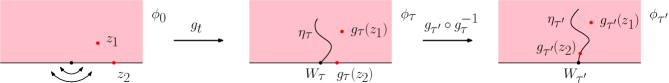
Figure 1: Let $\kappa\leq 4$ and $\gamma=\sqrt{\kappa}$. Left: Liouville field $\phi_{0}$ with insertions at $z_{1}\in\mathbbm{H}$ and $z_{2}\in\mathbbm{R}$. Middle: We conformally weld the left and right boundary arcs of $\phi_{0}$ according to quantum length to get $(\phi_{t},\eta_{t})_{t\geq 0}$. Time is parametrized by half-plane capacity of the curve. For a stopping time $\tau$ for $\mathcal{F}_{t}=\sigma(\eta_{t})$ such that $g_{\tau}(z_{2})$ has not yet hit the curve, Theorem 1.1 describes the law of $(\phi_{\tau},\eta_{\tau})$ in terms of the Liouville field and reverse SLE. Right: At the time $T$ that $g_{T}(z_{2})$ hits $W_{T}$, if the quantum length measure near $W_{T}$ is finite, we can continue the conformal welding process to “zip the marked point into the bulk”, e.g. until the depicted time $\tau^{\prime}$. Theorem 1.2 describes the law of $(\phi_{\tau^{\prime}},\eta_{\tau^{\prime}})$.

Theorem 1.1.

In the setting immediately above, assume $z_{1},\dots,z_{n}\neq 0$ and let $\tau$ be a stopping time with respect to the filtration $\mathcal{F}_{t}=\sigma(\eta_{t})$ such that a.s. $g_{\tau}(z_{j})\not\in\eta_{\tau}$ for all $j$. Let $I=\{i\>:\>z_{i}\in\mathbbm{H}\}$ and $B=\{b\>:\>z_{b}\in\mathbbm{R}\}$. Then the law of $(\phi_{\tau},\eta_{\tau})$ is

$$\prod_{i\in I}|g_{\tau}^{\prime}(z_{i})|^{2\Delta_{\alpha_{i}}}\prod_{b\in B}|g_{\tau}^{\prime}(z_{b})|^{\Delta_{2\alpha_{b}}}{{\mathrm{LF}}}_{\mathbbm{H}}^{(-\frac{1}{\sqrt{\kappa}},W_{\tau}),(\alpha_{j},g_{\tau}(z_{j}))_{j},(\delta,\infty)}(d\phi)\operatorname{rSLE}^{\tau}_{\kappa}(d\eta),$$

where $\Delta_{\alpha}:=\frac{\alpha}{2}(Q-\frac{\alpha}{2})$ and $\operatorname{rSLE}_{\kappa}^{\tau}$ is the law of reverse $\operatorname{SLE}_{\kappa}$ run until the stopping time $\tau$.

Informally, zipping up a Liouville field until a stopping time $\tau$ that depends only on the zipping interface, the curve $\eta_{\tau}$ is described by reverse $\operatorname{SLE}_{\kappa}$, and given $\eta_{\tau}$ the resulting field is described by a Liouville field with insertions at locations determined by $\eta_{\tau}$.

In Theorem 1.1 the condition that $g_{\tau}(z_{j})\not\in\eta_{\tau}$ for all $j$ is necessary, since otherwise the law of the curve would be singular with respect to reverse $\operatorname{SLE}_{\kappa}$. In Theorem 1.2, we allow boundary marked points to be zipped into the bulk, by using an $\operatorname{SLE}_{\kappa}$ variant called reverse $\operatorname{SLE}_{\kappa}$ with force points (see Section 2.3). Regardless, the zipping procedure can only be run until the continuation threshold, defined as the first time $t\leq\infty$ that any neighborhood of $W_{t}$ in $\mathbbm{R}$ has infinite quantum length, i.e. $\mathcal{L}_{\phi_{t}}((W_{t}-\varepsilon,W_{t}+\varepsilon))=\infty$ for all $\varepsilon>0$. Once the continuation threshold is hit, there is no canonical way to continue the conformal welding.

For finitely many $(a_{j},p_{j})\in\mathbbm{R}\times\overline{\mathbbm{H}}$ such that the points $p_{j}$ are distinct, we define

$$\mathcal{Z}((a_{j},p_{j})_{j})=\prod_{i\in I}(2\operatorname{Im}p_{i})^{-a_{i}^{2}/2}\prod_{j<k}e^{a_{j}a_{k}G(p_{j},p_{k})},\quad I=\{i:p_{i}\in\mathbbm{H}\},$$ (1.1)

where $G(p,q)=-\log|p-q|-\log|p-\overline{q}|$. If the $p_{j}$ are not distinct, we combine all pairs $(a,p)$ with the same $p$ by summing their $a$’s to get a collection $(a^{\prime}_{j},p^{\prime}_{j})$ with $p^{\prime}_{j}$ distinct, and define $\mathcal{Z}((a_{j},p_{j})_{j}):=\mathcal{Z}((a^{\prime}_{j},p^{\prime}_{j})_{j})$.

Theorem 1.2.

In the setting above Theorem 1.1, let $\tau$ be a stopping time with respect to the filtration $\mathcal{F}_{t}=\sigma(\eta_{t})$ which is not beyond the continuation threshold. Then the law of $(\phi_{\tau},\eta_{\tau})$ is

$$\frac{\mathcal{Z}((-\frac{1}{\sqrt{\kappa}},0),(\alpha_{j},z_{j})_{j})}{\mathcal{Z}((-\frac{1}{\sqrt{\kappa}},W_{\tau}),(\alpha_{j},g_{\tau}(z_{j}))_{j})}{{\mathrm{LF}}}_{\mathbbm{H}}^{(-\frac{1}{\sqrt{\kappa}},W_{\tau}),(\alpha_{j},g_{\tau}(z_{j}))_{j},(\delta,\infty)}(d\phi)\operatorname{rSLE}^{\tau}_{\kappa,\rho}(d\eta)$$ (1.2)

where $\operatorname{rSLE}_{\kappa,\rho}^{\tau}$ denotes the law of reverse $\operatorname{SLE}_{\kappa,\rho}$ with a force point at $z_{j}$ of weight $\rho_{j}=2\sqrt{\kappa}\alpha_{j}$ for each $j$, run until the stopping time $\tau$.

We emphasize that while we study the same Liouville field as e.g. [AHS22, ARS22, AS21, ASY22], for boundary insertions our notation differs by a factor of 2, see Remark 2.4. The present choice of notation simplifies the statement of Theorem 1.2 since boundary insertions zipped into the bulk maintain the same value of $\alpha$.

Remark 1.3.

Let $R_{t}:=\mathcal{Z}((-\frac{1}{\sqrt{\kappa}},0),(\alpha_{j},z_{j})_{j})/\mathcal{Z}((-\frac{1}{\sqrt{\kappa}},W_{t}),(\alpha_{j},g_{t}(z_{j}))_{j})$ be the prefactor in (1.2) at time $t$. If $\tau$ is a time such that $g_{\tau}(z_{j})=W_{\tau}$ for some $j$, then $\lim_{t\uparrow\tau}R_{t}\in\{0,\infty\}$ whereas $R_{\tau}\in(0,\infty)$. This apparent discontinuity is only cosmetic: the definition of ${{\mathrm{LF}}}_{\mathbbm{H}}^{(-\frac{1}{\sqrt{\kappa}},W_{t}),(\alpha_{j},g_{t}(z_{j}))_{j},(\delta,\infty)}$ includes a factor of $C_{\kappa}^{(-\frac{1}{\sqrt{\kappa}},W_{t}),(\alpha_{j},g_{t}(z_{j}))_{j},(\delta,\infty)}$ (defined in (2.2)), and $C_{\kappa}^{(-\frac{1}{\sqrt{\kappa}},W_{t}),(\alpha_{j},g_{t}(z_{j}))_{j},(\delta,\infty)}R_{t}$ is continuous in $t$.

1.3 The $\kappa\in(4,8)$ LCFT quantum zipper

We now need to work with beaded quantum surfaces which can have nontrivial topology. Suppose $(D,h)$ are such that $D\subset\mathbbm{C}$ is a closed set such that each connected component of the interior of $D$ and its prime-end boundary is homeomorphic to the closed disk, and $h$ is a generalized function defined only on the interior of $D$. We say that $(D,h)\sim_{\gamma}(\widetilde{D},\widetilde{h})$ if there is a homeomorphism $g:D\to\widetilde{D}$ which is conformal on each component of the interior of $D$ and which satisfies $\widetilde{h}=g\bullet_{\gamma}h$. A beaded quantum surface is an equivalence class of pairs $(D,h)$ under $\sim_{\gamma}$.

Let $\kappa\in(4,8)$ and $\gamma=\frac{4}{\sqrt{\kappa}}$. In this regime there is a natural beaded quantum surface called a rooted generalized quantum disk. It is obtained by sampling an excursion of a $\frac{\kappa}{4}$-stable Lévy process with no negative jumps, constructing a looptree whose nodes correspond to the jumps of the excursion, and for each node sampling an independent quantum disk with boundary length given by the jump size. This gives a beaded quantum surface with a marked boundary point, whose law is an infinite measure (since the Lévy excursion measure is infinite). Its boundary has a generalized quantum length measure coming from the time parametrization of the Lévy excursion.

A forested line is the beaded quantum surface obtained by attaching a Poissonian collection of marked generalized quantum disks to either the top or bottom of the half-line $(0,\infty)$. We equip the side without attached disks with a quantum length measure given by Lebesgue measure on $(0,\infty)$, whereas the other side inherits the generalized boundary length measure from the generalized quantum disks. The law of the forested line is a probability measure. For details on these constructions see [MSW21, Section 2.2] or [DMS21, Section 1.4.2].

A quantum wedge is a canonical scale-invariant $\gamma$-LQG surface with a weight parameter $W>0$. When $W\geq\frac{\gamma^{2}}{2}$ the quantum wedge is called thick and has the half-plane topology, and when $W<\frac{\gamma^{2}}{2}$ the quantum wedge is called thin and is the concatenation of a chain of countably many “beads”. See Section 2.4 for definitions.

Proposition 1.4 below states that there is a way to mate a pair of independent forested lines according to quantum forested length to obtain a beaded curve-decorated quantum surface.

Proposition 1.4 ([DMS21, Theorem 1.15]).

Sample a weight $(2-\frac{\gamma^{2}}{2})$ quantum wedge and let $\eta$ be a concatenation of independent $\operatorname{SLE}_{\kappa}(\frac{\kappa}{2}-4;\frac{\kappa}{2}-4)$ curves in each bead. Then $\eta$ divides the quantum wedge into two independent forested lines, whose forested boundaries are identified according to generalized quantum length. Moreover the curve-decorated quantum wedge is measurable with respect to the pair of forested lines.

We now explain a quantum zipper for the Liouville field with forested boundary, see Figure 2. Let $\mathrm{FL}_{\kappa}$ be the law of the pair of forested lines in Proposition 1.4 (so $\mathrm{FL}_{\kappa}$ is a probability measure). Let $n\geq 0$, let $(\alpha_{j},z_{j})\in\mathbbm{R}\times\overline{\mathbbm{H}}$ such that $z_{1},\dots,z_{n}$ are distinct, and let $\delta\in\mathbbm{R}$. Sample $(\phi_{0},(F_{L},F_{R}))\sim{{\mathrm{LF}}}_{\mathbbm{H}}^{(-\frac{1}{\sqrt{\kappa}},0),(\alpha_{j},z_{j})_{j},(\delta,\infty)}\times\mathrm{FL}_{\kappa}$ and glue $F_{L}$ (resp. $F_{R}$) to the boundary of $(\mathbbm{H},\phi_{0})$ according to quantum length, starting at $0$ and gluing to the left (resp. right). This gives a beaded quantum surface. For $s>0$ such that the generalized quantum lengths to the left and right of $0$ are at least $s$, let $p_{s}$ and $q_{s}$ be the forested boundary points to the left and right of $0$ having generalized quantum length $s$ from $0$. We mate the forested lines until we have identified $p_{s}$ and $q_{s}$, obtaining a curve-decorated beaded quantum surface (with the curve being the interface). We embed the curve-containing connected component via the hydrodynamic normalization, to get $(\mathbbm{H},\hat{\phi}_{s},\hat{\eta}_{s})$. That is, if $\hat{g}_{s}$ is the conformal map from $\mathbbm{H}$ to the unbounded connected component of $\mathbbm{H}\backslash\hat{\eta}_{s}$ satisfying $\lim_{z\to\infty}\hat{g}_{s}(z)-z=0$, then $\hat{g}_{s}^{-1}\bullet_{\gamma}\hat{\phi}_{s}=\phi_{0}$.

We reparametrize the process $(\hat{\phi}_{s},\hat{\eta}_{s},\hat{g}_{s})$ according to half-plane capacity to get $(\phi_{t},\eta_{t},g_{t})$ such that $\mathrm{hcap}(\eta_{t})=2t$. Let $W_{t}$ be the endpoint of $\eta_{t}$ lying in $\mathbbm{R}$. The continuation threshold is the first time $t\leq\infty$ that any neighborhood of $W_{t}$ has infinite generalized quantum length.

Figure 2: Let $\kappa\in(4,8)$ and $\gamma=\frac{4}{\sqrt{\kappa}}$. Left: We sample a Liouville field $\phi_{0}$ and attach independent forested lines to the left and right boundary arcs. Marked points are not depicted. Right: Mating the forested boundary arcs corresponds to “zipping up the quantum zipper”. The curve $\eta_{t}$ is the interface in $\mathbbm{H}$ between the purple and green forests. The conformal map $g_{t}$ sends the pink region on the left to that on the right and satisfies $\lim_{z\to\infty}g_{t}(z)-z=0$.

Theorem 1.5.

For $\kappa\in(4,8)$ and $\gamma=\frac{4}{\sqrt{\kappa}}$, the conclusions of Theorems 1.1 and 1.2 hold for the process $(\phi_{t},\eta_{t})$ constructed immediately above.

1.4 The $\kappa>8$ LCFT quantum zipper

In this section, we describe a mating of correlated continuum random trees. Let $(X_{t})_{t\geq 0}$ and $(Y_{t})_{t\geq 0}$ be correlated Brownian motions with $\operatorname{Var}(X_{t})=\operatorname{Var}(Y_{t})=\mathbbm{a}^{2}t$ and $\operatorname{Cov}(X_{t},Y_{t})=-\mathbbm{a}^{2}\cos(\frac{4\pi}{\kappa})t$ where $\mathbbm{a}^{2}=2/\sin(\frac{4\pi}{\kappa})$. We can construct a continuum random tree from $(X_{t})_{t\geq 0}$ by plotting the graph of $t\mapsto X_{t}$, letting $S\subset\mathbbm{R}^{2}$ be the set of points lying on or below the graph, and identifying points in $S$ which lie on a horizontal chord which stays below the graph; see Figure 3. In the same way we may construct a continuum random tree from $(Y_{t})_{t\geq 0}$, so $(X_{t},Y_{t})_{t\geq 0}$ describes a pair of correlated continuum random trees. We write $\mathrm{CRT}_{\kappa}$ for the law of $(X_{t},Y_{t})_{t\geq 0}$.

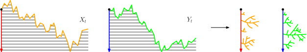
Figure 3: Left: Plot the graphs of the correlated Brownian motions $X_{t}$ and $Y_{t}$ (orange and green) and draw horizontal segments below the graphs (black). Right: Identifying points on the same horizontal segment gives a pair of correlated continuum random trees.

Recall that when $\kappa\geq 8$, the $\operatorname{SLE}_{\kappa}$ curve is space-filling. In this regime, the seminal mating-of-trees theorem of Duplantier, Miller and Sheffield can be stated as follows. See Figure 4.

Proposition 1.6.

Let $\kappa\geq 8$ and $\gamma=\frac{4}{\sqrt{\kappa}}$. Let $(\mathbbm{H},\phi,0,\infty,\eta)$ be an embedding of a weight $(2-\frac{\gamma^{2}}{2})$ quantum wedge decorated by an independent $\operatorname{SLE}_{\kappa}$ curve $\eta$. Parametrize $\eta$ by quantum area, so $A_{\phi}(\eta([0,t]))=t$. On the counterclockwise (resp. clockwise) boundary arc of $\eta([0,t])$ from $0$ to $\eta(t)$, let $X_{t}^{-}$ and $X_{t}^{+}$ (resp. $Y_{t}^{-}$ and $Y_{t}^{+}$) be the quantum lengths of the boundary segments in $\mathbbm{R}$ and $\mathbbm{H}$ respectively. Then the law of $(X_{t},Y_{t}):=(X_{t}^{+}-X_{t}^{-},Y_{t}^{+}-Y_{t}^{-})$ is $\mathrm{CRT}_{\kappa}$. Moreover, the curve-decorated quantum surface $(\mathbbm{H},\phi,0,\infty,\eta)/{\sim_{\gamma}}$ is measurable with respect to $(X_{t},Y_{t})_{t\geq 0}$.

The measurability statement and the fact that $(X_{t},Y_{t})$ evolve as correlated Brownian motion was shown in [DMS21], the correlation $\cos(\frac{\pi\gamma^{2}}{4})$ was obtained in [GHMS17], and the value of $\mathbbm{a}^{2}$ was identified in [ARS22]. (For the $\kappa\in(4,8)$ mating-of-trees theorem of [DMS21], see Proposition 7.6.)

Figure 4: Left: A pair of correlated continuum random trees. Right: There is a way of mating the pair of CRTs to get a weight $(2-\frac{\gamma^{2}}{2})$ quantum wedge decorated by an independent (space-filling) $\operatorname{SLE}_{\kappa}$ curve. Middle: Running the mating procedure until the quantum area is $t$, we write $X_{t}^{-},X_{t}^{+},Y_{t}^{-},Y_{t}^{+}$ for the quantum lengths of the red, orange, blue and green boundary arcs respectively, and set $(X_{t},Y_{t})=(X_{t}^{+}-X_{t}^{-},Y_{t}^{+}-Y_{t}^{-})$.

We can now state the quantum zipper for the Liouville field with correlated CRTs glued to the boundary, see Figure 5. Suppose $\kappa\geq 8$ and $\gamma=\frac{4}{\sqrt{\kappa}}$. Sample $(\phi_{0},(X_{t},Y_{t})_{t\geq 0})\sim{{\mathrm{LF}}}^{(-\frac{1}{\sqrt{\kappa}},0),(\alpha_{j},z_{j})_{j},(\delta,\infty)}\times\mathrm{CRT}_{\kappa}$ and let $X_{s}^{-}=-\inf_{u\leq s}X_{u}$ and $Y_{s}^{-}=-\inf_{u\leq s}Y_{u}$. For $s>0$ such that $L_{\phi_{0}}((-\infty,0))>X_{s}^{-}$ and $L_{\phi_{0}}((0,\infty))>Y_{s}^{-}$, let $a_{s}\in(-\infty,0)$ and $b_{s}\in(0,\infty)$ satisfy $L_{\phi_{0}}((a_{s},0))=X_{s}^{-}$ and $L_{\phi_{0}}((0,b_{s}))=Y_{s}^{-}$. Mate the pair of continuum random trees for $s$ units of quantum area to get a quantum surface with boundary arcs of lengths $X_{s}^{-},X_{s}^{+},Y_{s}^{-},Y_{s}^{+}$, and conformally weld the boundary arcs of lengths $X_{s}^{-}$ and $Y_{s}^{-}$ to the boundary arcs $(a_{s},0)$ and $(0,b_{s})$ of $(\mathbbm{H},\phi_{0})$ respectively. Embed the resulting curve-decorated quantum surface via the hydrodynamic normalization to get $(\mathbbm{H},\hat{\phi}_{s},\hat{\eta}_{s})$. That is, if $\hat{g}_{s}$ is the conformal map from $\mathbbm{H}$ to the unbounded connected component of $\mathbbm{H}\backslash\hat{\eta}_{s}$ satisfying $\lim_{z\to\infty}\hat{g}_{s}(z)-z=0$, then $\hat{g}_{s}^{-1}\bullet_{\gamma}\hat{\phi}_{s}=\phi_{0}$.

We reparametrize the process $(\hat{\phi}_{s},\hat{\eta}_{s},\hat{g}_{s})$ according to half-plane capacity to get $(\phi_{t},\eta_{t},g_{t})$ such that $\mathrm{hcap}(\eta_{t})=2t$. Let $W_{t}$ be the endpoint of $\eta_{t}$ lying in $\mathbbm{R}$. The continuation threshold is the first time $t$ that any neighborhood of $W_{t}$ in $\mathbbm{R}$ has infinite quantum length.

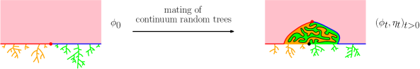
Figure 5: Let $\kappa\geq 8$ and $\gamma=\frac{4}{\sqrt{\kappa}}$. Left: We sample a Liouville field $\phi_{0}$ and attach correlated continuum random trees to the left and right boundaries. Marked points are not depicted. Right: Mating the trees corresponds to “zipping up the quantum zipper”. The curve $\eta_{t}$ is the interface in $\mathbbm{H}$ between the orange and green trees. The conformal map $g_{t}$ sends the pink region on the left to that on the right.

Theorem 1.7.

For $\kappa>8$ and $\gamma=\frac{4}{\sqrt{\kappa}}$, the conclusions of Theorems 1.1 and 1.2 hold for the process $(\phi_{t},\eta_{t})$ constructed immediately above.

Remark 1.8.

Theorem 1.7 should also hold for $\kappa=8$ but our argument does not apply to this critical value, see Remark 5.11. We leave the $\kappa=8$ LCFT quantum zipper as an open problem.

Remark 1.9.

Suppose $\kappa\in(4,8)$ and $\gamma=\frac{4}{\sqrt{\kappa}}$, and sample $(\phi_{0},(X_{t},Y_{t})_{t\geq 0})$ from ${{\mathrm{LF}}}^{(-\frac{1}{\sqrt{\kappa}},0),(\alpha_{j},z_{j})_{j},(\delta,\infty)}\times\mathrm{CRT}_{\kappa}$. For $s>0$, mating the continuum random trees for $s$ units of quantum area gives a beaded quantum surface, which a.s.  produces a non-simply-connected quantum surface when conformally welded with $(\mathbbm{H},\phi_{0})$. At the exceptional times $s$ that $X_{s}^{+}=Y_{s}^{+}=0$, however, the conformal welding yields a simply connected quantum surface. Restricting to these times and replacing the space-filling interfaces with non-space-filling curves measurable with respect to them, the result is the process described by Theorem 1.5. See Section 7.3 for more details.

1.5 BPZ equation for Liouville conformal field theory

We now give an application of the quantum zipper to LCFT, by proving a novel Belavin-Polyakov-Zamolodchikov (BPZ) equation for correlation functions with a degenerate boundary insertion.

In this section we distinguish bulk and boundary insertions with different letters. Let $m,n\geq 0$. Let $(\alpha_{j},z_{j})\in\mathbbm{R}\times\mathbbm{H}$ for $j\leq m$ and assume the $z_{j}$ are distinct. Let $-\infty=x_{0}<x_{1}<\dots<x_{n}<x_{n+1}=+\infty$ be boundary points, let $\beta_{1},\dots,\beta_{n}\in\mathbbm{R}$, and let $\delta\in\mathbbm{R}$. Let $\beta_{*}\in\{-\frac{\gamma}{2},-\frac{2}{\gamma}\}$.

For $k=0,\dots,n$ let $I_{k}=(x_{k},x_{k+1})$. Fix an index $k_{*}\in\{0,\dots,n\}$ and let $w\in I_{k_{*}}$. Let $I_{L}=(x_{k_{*}},w)$ and $I_{R}=(w,x_{k_{*}+1})$. See Figure 6. For $k\neq k_{*}$ let $\mu_{k}\in\mathbbm{C}$ satisfy $\operatorname{Re}\mu_{k}\geq 0$, and assume $\mu_{L},\mu_{R}\in\mathbbm{C}$ satisfy $\operatorname{Re}\mu_{L},\operatorname{Re}\mu_{R}\geq 0$ and are defined in terms of $\sigma_{L},\sigma_{R}\in\mathbbm{C}$ as follows:

$$\mu_{L}=g(\sigma_{L}),\,\,\mu_{R}=g(\sigma_{R})\quad\text{ where }g(\sigma)=\frac{\cos(\pi\gamma(\sigma-\frac{Q}{2}))}{\sqrt{\sin(\pi\gamma^{2}/4)}}\text{ and }\sigma_{L}-\sigma_{R}=\pm\frac{\beta_{*}}{2}.$$ (1.3)

Figure 6: Marked boundary points on $\partial\mathbbm{H}$ and the intervals between them. The bulk insertions are $(\alpha_{j},z_{j})_{j}$ (not depicted), the boundary insertions are $(\frac{\beta_{*}}{2},w),(\frac{\delta}{2},\infty)$ and $(\frac{\beta_{k}}{2},x_{k})$ for $1\leq k\leq n$. Each boundary interval $I_{\bullet}$ has an associated boundary cosmological constant $\mu_{\bullet}$.

Suppose the Seiberg bounds hold:

$$\sum_{j}\alpha_{j}+\sum_{k}\frac{\beta_{k}}{2}+\frac{\delta}{2}+\frac{\beta_{*}}{2}>Q,\qquad\alpha_{j},\beta_{k}<Q\text{ for all }j,k,\quad\delta<Q.$$ (1.4)

We define the LCFT correlation function $F_{\beta_{*}}(w,(z_{j})_{j},(x_{k})_{k})$ to be

$${{\mathrm{LF}}}_{\mathbbm{H}}^{(\frac{\beta_{*}}{2},w),(\alpha_{j},z_{j})_{j},(\frac{\beta_{k}}{2},x_{k}),(\frac{\delta}{2},\infty)}[\exp(-\mathcal{A}_{\phi}(\mathbbm{H})-\sum_{\begin{subarray}{c}0\leq k\leq n\\ k\neq k_{*}\end{subarray}}\mu_{k}\mathcal{L}_{\phi}(I_{k})-\mu_{L}\mathcal{L}_{\phi}(I_{L})-\mu_{R}\mathcal{L}_{\phi}(I_{R}))].$$ (1.5)

Because the Seiberg bounds hold, the integral (1.5) converges absolutely [HRV18, Theorem 3.1].

Theorem 1.10.

For $(\gamma,\beta_{*})\neq(\sqrt{2},-\frac{\gamma}{2})$, the correlation functions $F_{\beta_{*}}$ are smooth and satisfy the BPZ equation

$$\mathopen{}\mathclose{{}\left(\frac{1}{\beta_{*}^{2}}\partial_{ww}+\sum_{j}(\frac{1}{w-z_{j}}\partial_{z_{j}}+\frac{1}{w-\overline{z}_{j}}\partial_{\overline{z}_{j}})+\sum_{k}\frac{1}{w-x_{k}}\partial_{x_{k}}+\sum_{j}\operatorname{Re}\frac{2\Delta_{\alpha_{j}}}{(w-z_{j})^{2}}+\sum_{k}\frac{\Delta_{\beta_{k}}}{(w-x_{k})^{2}}}\right)F_{\beta_{*}}=0.$$

If we assume the $\kappa=8$ quantum zipper not proved in this paper, the proof of Theorem 1.10 carries through to the remaining case $(\gamma,\beta_{*})=(\sqrt{2},-\frac{\gamma}{2})$.

Here is a proof sketch. Consider the quantum zipper with $\kappa=\frac{4}{\beta_{*}^{2}}$, and let $A_{t},L_{t},R_{t}$ be the quantum area and left and right quantum boundary lengths at time $t$. For $\beta_{*}=-\frac{2}{\gamma}$ and $\kappa\leq 4$, the coupling of $\sigma_{L}$ and $\sigma_{R}$ gives $\mu_{L}+\mu_{R}=0$, so $\mu_{L}L_{t}+\mu_{R}R_{t}=\mu_{L}(L_{t}-R_{t})$. This quantity is invariant under the conformal welding zipper process, giving rise to an $\operatorname{SLE}_{\kappa}$ martingale from which the BPZ equation is immediate. For $\beta_{*}=-\frac{\gamma}{2}$ and $\kappa>4$, although $e^{-A_{t}-\mu_{L}L_{t}-\mu_{R}R_{t}}$ is not invariant, it evolves as a martingale (Lemma 7.3); the proof uses the mating-of-trees Brownian motion and requires the coupling (1.3). This again gives an $\operatorname{SLE}_{\kappa}$ martingale and thus the BPZ equation. These arguments only yield that $F_{\beta_{*}}$ is a weak solution, but a hypoellipticity argument following [Dub15, PW19] then implies that $F_{\beta_{*}}$ is smooth, completing the proof.

In their pioneering work, Belavin, Polyakov and Zamolodchikov used representation theoretic methods to derive BPZ equations for the sphere [BPZ84]. These were recently mathematically proved for LCFT [KRV19] using a subtle argument involving cancellations of not absolutely convergent integrals. See also [Rem20, RZ20, RZ22] for BPZ equations on the disk with bulk cosmological constant zero, that is, in (1.5) the term $-\mathcal{A}_{\phi}(\mathbbm{H})$ is removed.

When the bulk cosmological constant is nonzero, the BPZ equations do not hold unless there is a coupling of the cosmological constants $\mu_{L}$ and $\mu_{R}$ via (1.3). This was proposed by [FZZ00] after examining special cases. As far as we know, there was no prior conceptual explanation of this constraint, even in the physics literature. Our martingale argument explains (1.3).

Remark 1.11.

The statement of Theorem 1.10 was chosen for simplicity. Our argument is quite robust, and many of the conditions can be loosened.

• We can choose $\beta_{k}\geq Q$ if the boundary cosmological constants for the intervals adjacent to $x_{k}$ are zero. We can choose $\delta\geq Q$ if $\mu_{0}=\mu_{n}=0$.

• The condition that $\operatorname{Re}\mu_{k},\operatorname{Re}\mu_{L},\operatorname{Re}\mu_{R}\geq 0$ can be relaxed so long as (1.5) converges absolutely.

• The bound $\sum_{j}\alpha_{j}+\sum_{k}\frac{\beta_{k}}{2}+\frac{\delta}{2}+\frac{\beta_{*}}{2}>Q$ is needed to ensure convergence of (1.5). Sometimes the correlation function can be defined even when (1.5) is nonconvergent, by introducing truncations where the exponential in (1.5) is replaced by $e^{z}-1$ or $e^{z}-1-z$ for instance. See e.g. [AHS22, Proposition 3.4], [ARS22, (1.7)] and [Cer22, Theorem B].

We note that the smoothness result of Theorem 1.10 is itself rather nontrivial. [KRV19] proved the bulk correlation functions are $C^{2}$ using mollifications of the GFF, and this was extended to $C^{\infty}$ by [Oik19]. It is not clear to us whether these arguments can be adapted for boundary LCFT.

1.6 Outlook

We state here a few applications of the LCFT quantum zipper, and mention some future directions and open questions.

1.6.1 Integrability of boundary LCFT

The basic objects of conformal field theories are their correlation functions, and solving a conformal field theory means obtaining exact formulae for them. For the case of LCFT on surfaces without boundary, this was carried out in a series of landmark works that proved the three-point structure constant equals the DOZZ formula proposed in physics [KRV20], then made rigorous the conformal bootstrap program of physicists to recursively solve for all correlation functions on all surfaces [GKRV22, GKRV21].

A similar program is currently being carried out for LCFT on surfaces with boundary. With Remy and Sun we computed the one-point bulk structure constant using mating-of-trees [ARS22]. Taking the BPZ equation Theorem 1.10 as input, in future work with Remy, Sun and Zhu [ARSZ] we compute the boundary three-point structure constant and the bulk-boundary structure constant, making rigorous the formulas of Ponsot-Teschner [PT02] and Hosomichi [Hos01] respectively. Our work provides all the initial data needed to compute all correlation functions on surfaces with boundary. The boundary conformal bootstrap program has been initiated, see [Wu22].

1.6.2 Reversibility of whole plane $\operatorname{SLE}_{\kappa}$ when $\kappa>8$

For $\kappa\in(0,8]$, chordal SLE is reversible in the following sense. Let $f:\mathbbm{H}\to\mathbbm{H}$ be a conformal automorphism with $f(0)=\infty$ and $f(\infty)=0$. If $\eta$ is $\operatorname{SLE}_{\kappa}$ in $\mathbbm{H}$ from $0$ to $\infty$, then the time-reversal of $f\circ\eta$ has the same law as $\eta$ up to time-reparametrization [Zha08, MS16]. However, reversibility fails for $\kappa>8$ chordal $\operatorname{SLE}_{\kappa}$ [MS17].

Whole-plane SLE is a variant of SLE in $\mathbbm{C}$ that starts at $\infty$ and targets $0$. Its reversibility was established by [Zha15] for $\kappa\leq 4$ and [MS17] for $\kappa\in(4,8]$. For $\kappa>8$ the reversibility of whole-plane $\operatorname{SLE}_{\kappa}$ was conjectured in [VW20] via reversibility of the $\kappa\to\infty$ large deviations rate function, which they obtained from a field-foliation coupling they interpret as describing a “$\kappa\to\infty$ radial mating-of-trees”. Inspired by [VW20], in future work with Pu Yu we establish a radial mating-of-trees using the LCFT quantum zipper, then exploit mating-of-trees reversibility and LCFT reversibility to show whole-plane $\operatorname{SLE}_{\kappa}$ reversibility for $\kappa>8$.

1.6.3 A general theory of conformal welding in LCFT

It is known in many cases that conformally welding quantum surfaces described by LCFT produces a quantum surface also described by LCFT. This was first demonstrated for quantum wedges [She16], and many more cases followed [DMS21, HP21, MSW22, MSW21, AHS23, AHS22, ARS22, AS21, ASY22]. In all cases the welding interfaces are either chords or loops, and the surfaces have genus 0. In forthcoming work with Pu Yu, we will use the LCFT quantum zipper to obtain radial conformal weldings and subsequently develop a systematic framework that produces conformal weldings of quantum surfaces of arbitrary genus.

1.6.4 Other BPZ equations in random conformal geometry

Our argument uses the mating-of-trees framework to prove the boundary BPZ equation for LCFT on the disk. The BPZ equation for LCFT on the sphere has already been shown [KRV19], but can something similar to our proof of Theorem 1.10 give an alternative proof?

The conformal loop ensemble (CLE) [She09, SW12] is a canonical conformally invariant collection of loops that locally look like SLE [She09], and arises as the scaling limit of the collection of interfaces of statistical physics models. It is expected that CLE is described by a CFT – indeed a suitably-defined CLE three-point function agrees with the generalized minimal model CFT structure constant [AS21] – so CLE multipoint functions should satisfy the BPZ equations. In the present work we obtained the boundary LCFT BPZ equation from a BPZ equation for SLE (in the sense that using Itô calculus on the martingale of Lemma 3.1 gives a second-order differential equation resembling BPZ), using mating-of-trees. One might hope to turn this argument around: could a BPZ equation for CLE be obtained from the BPZ equation for LCFT [KRV19] using mating-of-trees?

Organization of the paper. In Section 2 we recall some preliminaries about LQG, LCFT, SLE and the mating-of-trees framework. In Section 3 we explain that reverse $\operatorname{SLE}_{\kappa,\rho}$ is reverse $\operatorname{SLE}_{\kappa}$ weighted by a GFF partition function. In Section 4 we adapt a Neumann GFF quantum zipper of [DMS21] to obtain the $\kappa\leq 4$ LCFT quantum zipper. In Section 5 we prove the $\kappa>8$ LCFT quantum zipper, and in Section 6 the $\kappa\in(4,8)$ LCFT quantum zipper. Finally, we establish the LCFT boundary BPZ equations in Section 7.

Acknowledgements. We thank Guillaume Remy, Xin Sun and Tunan Zhu for earlier discussions on alternative approaches towards proving the boundary LCFT BPZ equations. We thank Yoshiki Fukusumi, Xin Sun, Yilin Wang and Pu Yu for helpful discussions. The author was supported by the Simons Foundation as a Junior Fellow at the Simons Society of Fellows.

2 Preliminaries

2.1 The Gaussian free field and Liouville quantum gravity

Let $m$ be the uniform probability measure on the unit half-circle $\{z\>:\>z\in\mathbbm{H},|z|=1\}$. The Dirichlet inner product is defined by $\langle f,g\rangle_{\nabla}=(2\pi)^{-1}\int_{\mathbbm{H}}\nabla f\cdot\nabla g$. Consider the collection of smooth functions $f$ with $\langle f,f\rangle_{\nabla}<\infty$ and $\int f(z)m(dz)=0$, and let $H$ be its Hilbert space closure with respect to $\langle\cdot,\cdot\rangle_{\nabla}$. Let $(f_{n})$ be an orthonormal basis of $H$ and let $(\alpha_{n})$ be a collection of independent standard Gaussians. The summation

$$h=\sum_{n}\alpha_{n}f_{n}$$

a.s. converges in the space of distributions. Then $h$ is the Gaussian free field on $\mathbbm{H}$ normalized so $\int h(z)m(dz)=0$ [DMS21, Section 4.1.4].

Write $|z|_{+}:=\max(|z|,1)$. For $z,w\in\overline{\mathbbm{H}}$ we define

$$\begin{gathered}G_{\mathbbm{H}}(z,w)=-\log|z-w|-\log|z-\overline{w}|+2\log|z|_{+}+2\log|w|_{+},\\ G_{\mathbbm{H}}(z,\infty)=\lim_{w\to\infty}G_{\mathbbm{H}}(z,w)=2\log|z|_{+}.\end{gathered}$$ (2.1)

The GFF $h$ is the centered Gaussian field with covariance structure formally given by $\mathbbm{E}[h(z)h(w)]=G_{\mathbbm{H}}(z,w)$. This is formal because $h$ is a distribution and so does not admit pointwise values, but for smooth compactly supported functions $f,g$ on $\mathbbm{H}$ we have $\mathbbm{E}[(h,f)(h,g)]=\iint G_{\mathbbm{H}}(z,w)f(z)g(w)\,dz\,dw$.

Suppose $\phi=h+g$ where $g$ is a (random) function on $\mathbbm{H}$ which is continuous at all but finitely many points. Let $\phi_{\varepsilon}(z)$ denote the average of $\phi$ on $\partial B_{\varepsilon}(z)\cap\mathbbm{H}$. For $\gamma\in(0,2)$, the $\gamma$-LQG area measure $\mathcal{A}_{\phi}$ on $\mathbbm{H}$ can be defined by the almost sure weak limit $\mathcal{A}_{\phi}(dz)=\lim_{\varepsilon\to 0}\varepsilon^{\gamma^{2}/2}e^{\gamma\phi_{\varepsilon}(z)}dz$ [DS11]. Similarly, the $\gamma$-LQG boundary length measure $\mathcal{L}_{\phi}$ on $\mathbbm{R}$ can be defined by $\mathcal{L}_{\phi}(dx):=\lim_{\varepsilon\to 0}\varepsilon^{\gamma^{2}/4}e^{\frac{\gamma}{2}\phi_{\varepsilon}(x)}dx$. For the critical parameter $\gamma=2$ a correction is needed to make the measure nonzero; we set $\mathcal{A}_{\phi}(dz)=\lim_{\varepsilon\to 0}(\log(1/\varepsilon)-\phi_{\varepsilon}(z))\varepsilon^{2}e^{2\phi_{\varepsilon}(z)}dz$ and $\mathcal{L}_{\phi}(dz)=\lim_{\varepsilon\to 0}(\log(1/\varepsilon)-\frac{1}{2}\phi_{\varepsilon}(x))\varepsilon e^{\phi_{\varepsilon}(x)}dx$ [DRSV14]. See for instance [Lac22, Pow20] for more details.

2.2 The Liouville field

Let $\gamma\in(0,2]$ be the LQG parameter, and $Q=\frac{\gamma}{2}+\frac{2}{\gamma}$. Write $|z|_{+}:=\max(|z|,1)$.

Definition 2.1.

Let $(h,\mathbf{c})$ be sampled from $P_{\mathbbm{H}}\times[e^{-Qc}\,dc]$ and let $\phi(z)=h(z)-2Q\log|z|_{+}+\mathbf{c}$. We call $\phi$ the Liouville field on $\mathbbm{H}$ and denote its law by ${{\mathrm{LF}}}_{\mathbbm{H}}$.

Define

$$C_{\gamma}^{(\alpha,z)}=\mathopen{}\mathclose{{}\left\{\begin{array}[]{ll}|z|_{+}^{-2\alpha(Q-\alpha)}(2\operatorname{Im}z)^{-\alpha^{2}/2}&\mbox{if }z\in\mathbbm{H}\\ |z|_{+}^{-2\alpha(Q-\alpha)}&\mbox{if }z\in\mathbbm{R}\end{array}}\right..$$

For $\delta\in\mathbbm{R}$, $n\geq 0$ and $(\alpha_{j},z_{j})\in\mathbbm{R}\times\overline{\mathbbm{H}}$ for $j\leq n$ such that the $z_{j}$ are distinct, let

$$C_{\gamma}^{(\alpha_{j},z_{j})_{j},(\delta,\infty)}=\prod_{j}C_{\gamma}^{(\alpha_{j},z_{j})}e^{\alpha_{j}\delta G_{\mathbbm{H}}(z_{j},\infty)}\times\prod_{1\leq j<k\leq n}e^{\alpha_{j}\alpha_{k}G_{\mathbbm{H}}(z_{j},z_{k})}.$$ (2.2)

More generally, if the $(\alpha_{j},z_{j})$ are such that the $z_{j}$ are not distinct, we combine all pairs $(\alpha,z)$ with the same $z$ by summing their $\alpha$’s to get a collection $(\alpha^{\prime}_{j},z_{j}^{\prime})$ where the $z_{j}^{\prime}$ are distinct, and define $C_{\gamma}^{(\alpha_{j},z_{j})_{j},(\delta,\infty)}=C_{\gamma}^{(\alpha_{j}^{\prime},z_{j}^{\prime})_{j},(\delta,\infty)}$.

Definition 2.2.

For $\delta\in\mathbbm{R}$, $n\geq 0$ and $(\alpha_{j},z_{j})\in\mathbbm{R}\times\overline{\mathbbm{H}}$, let $(h,\mathbf{c})$ be sampled from $C^{(\alpha_{j},z_{j})_{j},(\delta,\infty)}_{\gamma}P_{\mathbbm{H}}\times[e^{(\sum_{j}\alpha_{j}+\delta-Q)c}\,dc]$, and set

$$\phi(z)=h(z)+\sum_{j}\alpha_{j}G_{\mathbbm{H}}(z,z_{j})+(\delta-Q)G_{\mathbbm{H}}(z,\infty)+\mathbf{c}.$$

We call $\phi$ the Liouville field with insertions $(\alpha_{j},z_{j})_{j}$, $(\delta,\infty)$ and we write ${{\mathrm{LF}}}_{\mathbbm{H}}^{(\alpha_{j},z_{j})_{j},(\delta,\infty)}$ for its law.

Note that ${{\mathrm{LF}}}_{\mathbbm{H}}^{(\alpha_{j},z_{j})_{j},(\delta,\infty)}$ depends implicitly on the parameter $\gamma$. When $\delta=0$ there is no insertion at $\infty$, so we write $C_{\gamma}^{(\alpha_{j},z_{j})_{j}}$ and ${{\mathrm{LF}}}_{\mathbbm{H}}^{(\alpha_{j},z_{j})_{j}}$ rather than $C_{\gamma}^{(\alpha_{j},z_{j})_{j},(0,\infty)}$ and ${{\mathrm{LF}}}_{\mathbbm{H}}^{(\alpha_{j},z_{j})_{j},(0,\infty)}$.

Remark 2.3.

When $\sum_{j}\alpha_{j}+\delta=Q$, Definition 2.2 has the following simplification. Sample $(h,\mathbf{c})\sim C^{(\alpha_{j},z_{j})_{j},(\delta,\infty)}_{\gamma}P_{\mathbbm{H}}\times dc$, and let

$$\phi(z)=h(z)+\sum_{j}\alpha_{j}G(z,z_{j})+\mathbf{c}$$ (2.3)

where $G(z,w)=-\log|z-w|-\log|z-\overline{w}|$. Then the law of $\phi$ is ${{\mathrm{LF}}}_{\mathbbm{H}}^{(\alpha_{j},z_{j})_{j},(\delta,\infty)}$. Moreover, we have the simplification $C^{(\alpha_{j},z_{j})_{j},(\delta,\infty)}_{\gamma}=\mathcal{Z}((\alpha_{j},z_{j})_{j})$ with $\mathcal{Z}$ defined in and below (1.1).

Remark 2.4.

Let $m,n\geq 0$, let $(\alpha_{j},z_{j})\in\mathbbm{R}\times\mathbbm{H}$ for $j\leq m$, let $(\beta_{k},x_{k})\in\mathbbm{R}\times\mathbbm{R}$ for $k\leq n$, and let $\beta\in\mathbbm{R}$. The measure that we call ${{\mathrm{LF}}}_{\mathbbm{H}}^{(\alpha_{j},z_{j})_{j},(\frac{1}{2}\beta_{k},x_{k})_{k},(\frac{1}{2}\beta,\infty)}$ is instead called “$\mathrm{LF}_{\mathbbm{H}}^{(\alpha_{j},z_{j})_{j},(\beta_{k},x_{k})_{k},(\beta,\infty)}$” in [AHS22, ARS22]; there, the boundary insertions are described by their log-singularities (near $x_{k}$ the field blows up as $-\beta_{k}\log|\cdot-x_{k}|$), whereas our notation instead uses the Green function coefficient (near $x_{k}$ the field blows up like $\frac{\beta_{k}}{2}G_{\mathbbm{H}}(\cdot,x_{k})$). Our notation is more convenient for this paper since the Green function coefficient is invariant when a boundary point is zipped into the bulk.

Finally, we will need the following rooted measure statement: sampling a point from the quantum area measure of a Liouville field is equivalent to adding a $\gamma$-insertion to the field.

Proposition 2.5.

Suppose $\gamma\in(0,2)$. Let $n\geq 0$ and $(\alpha_{j},z_{j})\in\mathbbm{R}\times\overline{\mathbbm{H}}$ for $j\leq n$, and let $\delta\in\mathbbm{R}$. Then

$$\mathcal{A}_{\phi}(dz)\,{{\mathrm{LF}}}_{\mathbbm{H}}^{(\alpha_{j},z_{j})_{j},(\delta,\infty)}(d\phi)={{\mathrm{LF}}}_{\mathbbm{H}}^{(\alpha_{j},z_{j})_{j},(\gamma,z),(\delta,\infty)}(d\phi)\,dz.$$

Formally, Proposition 2.5 holds because $\mathcal{A}_{\phi}(dz)=\lim_{\varepsilon\to 0}\varepsilon^{\gamma^{2}/2}e^{\gamma\phi_{\varepsilon}(z)}dz$ and ${{\mathrm{LF}}}_{\mathbbm{H}}^{(\alpha_{j},z_{j})_{j},(\gamma,z),(\delta,\infty)}(d\phi)=\lim_{\varepsilon\to 0}\varepsilon^{\gamma^{2}/2}e^{\gamma\phi_{\varepsilon}(z)}{{\mathrm{LF}}}_{\mathbbm{H}}^{(\alpha_{j},z_{j})_{j},(\delta,\infty)}(d\phi)$, where $\phi_{\varepsilon}(z)$ is the average of $\phi$ on $\partial B_{\varepsilon}(z)\cap\mathbbm{H}$. A rigorous proof of the analogous statement for $\mathbbm{C}$ is given in [AHS22, Lemma 2.31]; the proof of Proposition 2.5 is identical so we omit it.

2.3 Reverse Schramm-Loewner evolution

In this section we recall some basic properties of SLE, see [Kem17] for a more detailed introduction. Let $\kappa>0$. Let $\rho_{1},\dots,\rho_{n}\in\mathbbm{R}$ and let $z_{1},\dots,z_{n}\in\overline{\mathbbm{H}}$ be distinct points. With $(B_{t})_{t\geq 0}$ a standard Brownian motion, the driving function $(W_{t})_{t\geq 0}$ for reverse $\operatorname{SLE}_{\kappa,\rho}$ is defined by the stochastic differential equations

$$\begin{gathered}W_{0}=0,\quad dW_{t}=\sum_{j=1}^{n}\operatorname{Re}\mathopen{}\mathclose{{}\left(\frac{-\rho_{j}}{Z^{j}_{t}-W_{t}}}\right)\,dt+\sqrt{\kappa}\,dB_{t},\\ Z^{j}_{0}=z_{j},\quad dZ^{j}_{t}=-\frac{2}{Z^{j}_{t}-W_{t}}\,dt\quad\text{for }j=1,\dots,n.\end{gathered}$$ (2.4)

For each $z\in\mathbbm{H}$ and $s\geq 0$, let $(g_{s,t}(z))_{t\geq s}$ be the solution to $g_{s,s}(z)=z$, $\frac{d}{dt}g_{s,t}(z)=-\frac{2}{g_{s,t}(z)-W_{t}}$. This defines a family of conformal maps $g_{s,t}$; we also write $g_{t}:=g_{0,t}$. For each $t>0$ we can define a curve $\eta_{t}:[0,t]\to\overline{\mathbbm{H}}$ by $\eta_{t}(u):=\lim_{z\to W_{t-u}}g_{t-u,t}(z)$. We call the family of curves $(\eta_{t})_{t\geq 0}$ reverse $\operatorname{SLE}_{\kappa}$ with force points at $z_{j}$ of weight $\rho_{j}$. Note that $g_{t}$ is the unique conformal map from $\mathbbm{H}$ to the unbounded connected component of $\mathbbm{H}\backslash\eta_{t}$ such that $\lim_{z\to\infty}g_{t}(z)-z=0$, and that reverse SLE is parametrized by half-plane capacity in the sense that $\mathrm{hcap}(\eta_{t}):=\lim_{z\to\infty}z(g_{t}(z)-z)$ equals $2t$. The curve $\eta_{t}$ is simple when $\kappa\leq 4$, self-intersecting (but not self-crossing) when $\kappa\in(4,8)$, and space-filling when $\kappa\geq 8$.

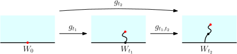
Figure 7: Reverse $\operatorname{SLE}_{\kappa}$ for $\kappa\leq 4$; similar diagrams with different topologies can be drawn for $\kappa\in(4.8)$ and $\kappa\geq 8$. The curve grows from its base. As depicted, $\eta_{t}(0)=W_{t}$ and $\eta_{t}(t)=\lim_{z\to W_{0}}g_{t}(z)$.

In the case of no force points ($n=0$), this process is well-defined for all time. For $n\geq 0$, by absolute continuity with respect to the $n=0$ case, the SDE (2.4) can be run until the time $\tau$ that $g_{t}(z_{j})=W_{t}$ for some $j$. Let $J_{\tau}=\{j\>:\>g_{\tau}(z_{j})=W_{\tau}\}$. If $\sum_{j\in J_{\tau}}\rho_{j}<\frac{\kappa}{2}+4$, then there is a unique way of continuing the process such that $g_{t}(z_{j})\in\mathbbm{H}$ for all $t>\tau$ [DMS21, Proposition 3.8]. Applying this continuation procedure to each time a force point hits $W_{t}$, we see that reverse $\operatorname{SLE}_{\kappa,\rho}$ is well-defined until the continuation threshold: the first time $\tau\leq\infty$ that the sum of the weights of force points hitting $W_{\tau}$ is at least $\frac{\kappa}{2}+4$.

2.4 Quantum wedges and quantum cells

In this section we define the quantum wedges introduced in [She16, DMS21], and the quantum cell which arises from partially mating correlated continuum random trees.

We first define quantum wedges. For symmetry reasons it is easier to work in the strip $\mathcal{S}:=\mathbbm{R}\times(0,\pi)$ than in $\mathbbm{H}$. Let $m$ be the uniform probability measure on the segment $\{0\}\times(0,\pi)$. As in Section 2.1, consider the space of smooth functions $f$ on $\mathcal{S}$ with $\langle f,f\rangle_{\nabla}$ and $\int f(z)m(dz)=0$, and let $H$ be the Hilbert space closure with respect to $\langle\cdot,\cdot\rangle_{\nabla}$. As before, let $h=\sum_{j}\alpha_{j}f_{j}$ where the $\alpha_{j}$ are i.i.d. standard Gaussians and $\{f_{j}\}$ is an orthonormal basis for $H$. We call $h$ the GFF on $\mathcal{S}$ normalized so $\int h(z)m(dz)=0$, and denote its law by $P_{\mathcal{S}}$.

We can decompose $H=H_{\mathrm{av}}\oplus H_{\mathrm{lat}}$ where $H_{\mathrm{av}}$ (resp. $H_{\mathrm{lat}}$) is the subspace of functions which are constant (resp. have mean zero) on $\{t\}\times(0,\pi)$ for all $t\in\mathbbm{R}$; this gives a decomposition $h=h_{\mathrm{av}}+h_{\mathrm{lat}}$ of $h$ into independent components.

We now define thick quantum wedges. These are $\gamma$-LQG surfaces with the half-plane topology, and have a weight parameter $W\geq\frac{\gamma^{2}}{2}$.

Definition 2.6 (Thick quantum wedge).

For $W\geq\frac{\gamma^{2}}{2}$, let $\alpha=\frac{1}{2}(Q+\frac{\gamma}{2}-\frac{W}{\gamma})$. Let

$$Y_{t}=\mathopen{}\mathclose{{}\left\{\begin{array}[]{ll}B_{2t}+(Q-2\alpha)t&\mbox{if }t\geq 0\\ \widetilde{B}_{-2t}+(Q-2\alpha)t&\mbox{if }t<0\end{array}}\right.$$

where $(B_{s})_{s\geq 0}$ is standard Brownian motion, and independently $(\widetilde{B}_{s})_{s\geq 0}$ is standard Brownian motion conditioned on $\widetilde{B}_{2s}-(Q-2\alpha)s<0$ for all $s>0$. Let $\phi_{\mathrm{av}}(z)=Y_{\operatorname{Re}z}$, let $\phi_{\mathrm{lat}}$ be the projection of an independent GFF onto $H_{\mathrm{lat}}$, and let $\phi_{0}=\phi_{\mathrm{av}}+\phi_{\mathrm{lat}}$. We call the quantum surface $(\mathcal{S},\phi_{0},-\infty,+\infty)/{\sim_{\gamma}}$ a weight $W$ quantum wedge and write $\mathcal{M}^{\mathrm{wed}}(W)$ for its law.

Thin quantum wedges are an ordered collection of two-pointed quantum surfaces.

Definition 2.7 (Thin quantum wedge).

For $W\in(0,\frac{\gamma^{2}}{2})$, sample a Bessel process of dimension $\delta=1+\frac{2W}{\gamma^{2}}$. It decomposes as a countable ordered collection of Bessel excursions; for each excursion $e$ we construct a two-pointed quantum surface $\mathcal{B}_{e}=(\mathcal{S},\phi^{e},-\infty,\infty)/{\sim_{\gamma}}$ as follows. Let $(Y_{t}^{e})_{t\in\mathbbm{R}}$ be any time-reparametrization of $\frac{2}{\gamma}\log e$ which has quadratic variation $2dt$. Let $\phi_{\mathrm{av}}^{e}(z)=Y_{\operatorname{Re}z}^{e}$, let $\phi^{e}_{\mathrm{lat}}$ be the projection of a GFF (independent of everything else) onto $H_{\mathrm{lat}}$, and set $\phi^{e}=\phi_{\mathrm{av}}^{e}+\phi_{\mathrm{lat}}^{e}$. Then the weight $W$ quantum wedge is the ordered collection $(\mathcal{B}_{e})$.

Now, to avoid topological complications, assume $\gamma\in(0,\sqrt{2}]$ and $\kappa=\frac{16}{\gamma^{2}}$. Let $(\mathbbm{H},h,0,\infty)$ be an embedding of a sample from $\mathcal{M}^{\mathrm{wed}}(2-\frac{\gamma^{2}}{2})$. Let $\eta$ be an independent $\operatorname{SLE}_{\kappa}$ from $0$ to $\infty$; parametrize $\eta$ by quantum area so $\mathcal{A}_{h}(\eta([0,a]))=a$ for all $a>0$. Let $D_{a}=\eta([0,a])$ and let $p=\eta(0)$ and $q=\eta(a)$. Let $x_{L}$ (resp. $x_{R}$) be the last point on the left (resp. right) boundary arc of $\mathbbm{H}$ hit by $\eta$ before time $a$.

Definition 2.8.

We call the $\operatorname{SLE}_{\kappa}$-decorated quantum surface $\mathcal{C}_{a}=(D_{a},h,\eta|_{[0,a]},p,q,x_{L},x_{R})/{\sim_{\gamma}}$ an area $a$ quantum cell. We denote its law by $P_{a}$.

Recall that there is a way of mating correlated continuum random trees to obtain LQG decorated by SLE, see Proposition 1.6. By its definition, the area $a$ quantum cell is the decorated quantum surface arising from mating a pair of correlated Brownian motions $(X_{t},Y_{t})_{t\geq 0}\sim\mathrm{CRT}_{\kappa}$ and stopping when the quantum area is $a$.

Remark 2.9.

When $(\gamma,\kappa)\neq(\sqrt{2},8)$, the quantum cell $\mathcal{C}_{a}$ is measurable with respect to $(D_{a},h,\eta|_{[0,a]})/{\sim_{\gamma}}$, that is, the four marked points can be recovered from $(D_{a},h,\eta|_{[0,a]})/{\sim_{\gamma}}$. First, we can recover two of the marked points $p=\eta(0)$ and $q=\eta(a)$. Let $\psi:D_{a}\to\mathbbm{H}$ be a conformal map with $\psi(p)=0$ and $\psi(q)=\infty$. From the imaginary geometry construction of space-filling $\operatorname{SLE}_{\kappa}$ [MS17], modulo time-parametrization the law of $\psi\circ\eta$ given $\psi(x_{L})$ and $\psi(x_{R})$ is $\operatorname{SLE}_{\kappa,\rho}$ with force points of size $\kappa/2-4$ at $\psi(x_{L})$ and $\psi(x_{R})$. Since $\kappa/2-4\neq 0$ the points $\psi(x_{L})$ and $\psi(x_{R})$ are measurable with respect to $\psi\circ\eta$, so we can recover $x_{L}$ and $x_{R}$ also. In this paper, we will not consider the $(\gamma,\kappa)=(\sqrt{2},8)$ case, so for notational simplicity we will frequently omit the marked points.

Since Brownian motion is reversible, it is unsurprising that the area $a$ quantum cell is reversible:

Lemma 2.10.

$\mathcal{C}_{a}$ is symmetric in law in the following sense. If $\widetilde{\eta}$ is the time-reversal of $\eta|_{[0,a]}$, then $(D_{a},h,\eta|_{[0,a]},p,q,x_{L},x_{R})/{\sim_{\gamma}}$ and $(D_{a},h,\widetilde{\eta},q,p,x_{R},x_{L})/{\sim_{\gamma}}$ have the same law.

Proof.

[DMS21, Theorem 1.9] states that if a $\gamma$-quantum cone $(\mathbbm{C},h,0,\infty)/{\sim_{\gamma}}$ is decorated by an independent $\operatorname{SLE}_{\kappa}$ curve $\eta$ from $\infty$ to $\infty$, then parametrizing $\eta:\mathbbm{R}\to\mathbbm{C}$ by quantum area and fixing $\eta(0)=0$, the quantum surface $(\eta((0,\infty)),h,0,\infty)/{\sim_{\gamma}}$ has law $\mathcal{M}^{\mathrm{wed}}(2-\frac{\gamma^{2}}{2})$. Thus $(\eta([0,a]),h,\eta|_{[0,a]})/{\sim_{\gamma}}$ has law $P_{a}$. Let $z=\eta(a)$, then [DMS21, Theorem 1.9] states that $(\mathbbm{C},h(\cdot+z),\eta(\cdot+a)-z)/{\sim_{\gamma}}$ also has the law of a $\gamma$-quantum cone decorated by an independent $\operatorname{SLE}_{\kappa}$ from $\infty$ to $\infty$, and by the reversibility of this $\operatorname{SLE}_{\kappa}$ curve, the decorated quantum surface $(\mathbbm{C},h(\cdot+z),\eta(a-\cdot)-z)/{\sim_{\gamma}}$ also has this law. Thus, $(\eta([0,a]),h,\tilde{\eta})$ also has law $P_{a}$, where $\tilde{\eta}:[0,a]\to\mathbbm{C}$ is given by $\tilde{\eta}(t)=\eta(a-t)$. ∎

3 Reverse $\operatorname{SLE}_{\kappa,\rho}$ and the GFF partition function

We make no claim of originality for the material in this section, and present it here for completeness. See the end of this section for references.

Let $n\geq 0$ and let $(\alpha_{j},z_{j})\in\mathbbm{R}\times\overline{\mathbbm{H}}$ for $j\leq n$, where the $z_{j}$ are distinct. Let $w\in\mathbbm{R}$. Let $\kappa>0$, $\gamma=\min(\sqrt{\kappa},\frac{4}{\sqrt{\kappa}})$. The GFF partition function $\mathcal{Z}$ defined in (1.1), times a factor arising from uniformizing in $\mathbbm{H}$, is a martingale observable for reverse SLE:

Lemma 3.1.

Let $\kappa>0$. Let $n\geq 0$, and let $(\alpha_{j},z_{j})\in\mathbbm{R}\times\overline{\mathbbm{H}}$ for $j\leq n$. Let $I=\{j:z_{j}\in\mathbbm{H}\}$ and $B=\{j:z_{j}\in\mathbbm{R}\}$. Sample reverse $\operatorname{SLE}_{\kappa}$ with no force points (as in (2.4)) and define

$$M_{t}=\prod_{i\in I}|g_{t}^{\prime}(z_{i})|^{2\Delta_{\alpha_{i}}}\prod_{b\in B}|g_{t}^{\prime}(z_{b})|^{\Delta_{2\alpha_{b}}}\mathcal{Z}\big{(}(-\frac{1}{\sqrt{\kappa}},W_{t}),(\alpha_{j},g_{t}(z_{j}))_{j}\big{)}$$

where $\Delta_{\alpha}:=\frac{\alpha}{2}(Q-\frac{\alpha}{2})$ and $Q=\frac{\gamma}{2}+\frac{2}{\gamma}$. Let $\tau$ be a stopping time such that almost surely $g_{t}(z_{j})\neq W_{t}$ for all $t\leq\tau$. Then $M_{t}$ is a martingale up until time $\tau$.

Proof.

To lighten notation, we assume there are only bulk insertions (i.e. $z_{j}\in\mathbbm{H}$ for all $j$); the general case follows from the same arguments. We write $Z_{j}=g_{t}(z_{j})$ and write $W=W_{t}$, leaving the $t$-dependence implicit to simplify notation. Our goal is to compute $d\log M_{t}$. We have

$$\log M_{t}= \sum_{j}2\Delta_{\alpha_{j}}\log|g_{t}^{\prime}(z_{j})|-\frac{\alpha_{j}^{2}}{2}\log(2\operatorname{Im}Z_{j})+\frac{2\alpha_{j}}{\sqrt{\kappa}}\log|Z_{j}-W|+\sum_{1\leq j<k\leq m}\alpha_{j}\alpha_{k}G(Z_{j},Z_{k}).$$ (3.1)

By the definition of the reverse Loewner flow and $Z_{j}=g_{t}(z_{j})$, we have

$$dW=\sqrt{\kappa}dB_{t},\enspace d\langle W\rangle=\kappa dt,\enspace dZ_{j}=-\frac{2dt}{Z_{j}-W},\enspace d\overline{Z}_{j}=-\frac{2dt}{\overline{Z}_{j}-W},\enspace d\log|g_{t}^{\prime}(z_{j})|=\operatorname{Re}\frac{2dt}{(Z_{j}-W)^{2}}.$$

The last identity holds since $d(g_{t}(z))=-\frac{2}{g_{t}(z)-W}dt$ implies $d(g_{t}^{\prime}(z))=-\frac{2}{(g_{t}(z)-W)^{2}}g_{t}^{\prime}(z)dt$. Using these we have $d\log(2\operatorname{Im}Z_{j})=d\log(Z_{j}-\overline{Z}_{j})=\frac{1}{Z_{j}-\overline{Z}_{j}}dZ_{j}+\frac{1}{\overline{Z}_{j}-Z_{j}}d\overline{Z}_{j}=\frac{1}{|Z_{j}-W|^{2}}dt$ and, since $\log|Z_{j}-W|=\operatorname{Re}\log(Z_{j}-W)$, we have $d\log|Z_{j}-W|=\operatorname{Re}\frac{\sqrt{\kappa}}{W-Z_{j}}dB_{t}-\operatorname{Re}\frac{\sqrt{\kappa}Q}{(W-Z_{j})^{2}}dt$. Thus

$$d\mathopen{}\mathclose{{}\left(2\Delta_{\alpha_{j}}\log|g_{t}^{\prime}(z_{j})|-\frac{\alpha_{j}^{2}}{2}\log(2\operatorname{Im}Z_{j})+\frac{2\alpha_{j}}{\sqrt{\kappa}}\log|Z_{j}-W|}\right)$$ (3.2)

$$=\operatorname{Re}\frac{2\alpha_{j}}{W-Z_{j}}dB_{t}-(\operatorname{Re}\frac{1}{(Z_{j}-W)^{2}}+\frac{1}{|Z_{j}-W|^{2}})\alpha_{j}^{2}dt=\operatorname{Re}\frac{2\alpha_{j}}{W-Z_{j}}dB_{t}-2\alpha_{j}^{2}\mathopen{}\mathclose{{}\left(\operatorname{Re}\frac{1}{Z_{j}-W}}\right)^{2}dt.$$

In the last equality, we used the identity $\operatorname{Re}(z^{2})+|z|^{2}=2(\operatorname{Re}z)^{2}$. Next, since $G(Z_{j},z)=-\operatorname{Re}(\log(Z_{j}-z)+\log(Z_{j}-\overline{z}))$, we have $dG(Z_{j},z)=\operatorname{Re}\mathopen{}\mathclose{{}\left((\frac{1}{Z_{j}-z}+\frac{1}{Z_{j}-\overline{z}})\frac{2}{Z_{j}-W}}\right)dt$, so

$$d G(Z_{j},Z_{k})=\operatorname{Re}\mathopen{}\mathclose{{}\left((\frac{1}{Z_{j}-Z_{k}}+\frac{1}{Z_{j}-\overline{Z}_{k}})\frac{2}{Z_{j}-W}+(\frac{1}{Z_{k}-Z_{j}}+\frac{1}{Z_{k}-\overline{Z}_{j}})\frac{2}{Z_{k}-W}}\right)dt$$

$$=\operatorname{Re}\mathopen{}\mathclose{{}\left(-\frac{2}{(Z_{j}-W)(Z_{k}-W)}-\frac{2}{(Z_{j}-W)(\overline{Z}_{k}-W)}}\right)dt=-4\operatorname{Re}\mathopen{}\mathclose{{}\left(\frac{1}{Z_{k}-W}}\right)\operatorname{Re}\mathopen{}\mathclose{{}\left(\frac{1}{Z_{j}-W}}\right)dt.$$

Combining this with (3.2), we can compute $d\log M_{t}$ from (3.1):

$$d\log M_{t}=(\sum_{j}\operatorname{Re}\frac{2\alpha_{j}}{W-Z_{j}})dB_{t}-\frac{1}{2}(\sum_{j}\operatorname{Re}\frac{2\alpha_{j}}{W-Z_{j}})^{2}dt.$$

Thus, $M_{t}$ is a martingale, completing the proof for the case of only bulk insertions. The general case is essentially the same: we get the same expression for $d\log M_{t}$ so $M_{t}$ is a martingale. ∎

Proposition 3.2.

In the setting of Lemma 3.1, the law of reverse $\operatorname{SLE}_{\kappa}$ run until $\tau$ and weighted by $\frac{M_{\tau}}{M_{0}}$ is precisely that of $\operatorname{SLE}_{\kappa,\rho}$ run until the stopping time $\tau$, where at each $z_{j}$ there is a force point of weight $\rho_{j}=2\sqrt{\kappa}\alpha_{j}$.

Proof.

We use the notation ${\mathcal{Z}_{\kappa}^{\alpha}}(w,(z_{j})_{j}):=\mathcal{Z}((-\frac{1}{\sqrt{\kappa}},w),(\alpha_{j},z_{j})_{j})$. By Girsanov’s theorem, under the reweighted law, the driving function satisfies the SDE

$$dW_{t}=\sqrt{\kappa}\,dB_{t}+\kappa\partial_{w}\log{\mathcal{Z}_{\kappa}^{\alpha}}(W_{t},(g_{t}(z_{j}))_{j})dt.$$

We have $\partial_{w}\log{\mathcal{Z}_{\kappa}^{\alpha}}(w,(z_{j})_{j})=\sum_{j}-\frac{2}{\sqrt{\kappa}}\alpha_{j}\partial_{w}\operatorname{Re}\log(z_{j}-w)=\sum_{j}\operatorname{Re}\mathopen{}\mathclose{{}\left(\frac{-2\alpha_{j}/\sqrt{\kappa}}{z_{j}-w}}\right)$, so the SDE agrees with (2.4) as desired. ∎

The observation that reverse SLE with force points is intimately related to the Coulomb gas partition function is not original. See for instance [Fuk17, Ale19, KK20, KM21, Kos21]. A similar perspective arose earlier in the setting of forward SLE. See e.g. [BB03, BBK05, Kyt06].

4 Sheffield’s coupling and the $\kappa\leq 4$ LCFT zipper

In this section we prove Theorems 1.1 and 1.2. These results are fairly straightforward consequences of Sheffield’s coupling of LQG and SLE.

A version of the following was first proved in [She16], and the full version where force points may be zipped into the bulk was proved in [DMS21]. Recall $G(z,w)=-\log|z-w|-\log|z-\overline{w}|$.

Proposition 4.1 ([DMS21, Theorem 5.1]).

Let $\kappa>0$, $\gamma=\min(\sqrt{\kappa},\frac{4}{\sqrt{\kappa}})$, let $n\geq 0$ and $(\rho_{j},z_{j})\in\mathbbm{R}\times\overline{\mathbbm{H}}$ for $j\leq n$. Suppose that $(W_{t})_{t\geq 0}$ is the driving function for reverse $\operatorname{SLE}_{\kappa,\rho}$ with force points at $z_{j}$ of size $\rho_{j}$, and let $g_{t}$ be the Loewner map. For each $t\geq 0$ let

$${\mathfrak{h}}_{t}(z)=-\frac{1}{\sqrt{\kappa}}G(z,W_{t})+\frac{1}{2\sqrt{\kappa}}\sum_{j=1}^{n}\rho_{j}G(g_{t}(z),g_{t}(z_{j}))+Q\log|g_{t}^{\prime}(z)|.$$

Let $h$ be an independent Neumann GFF modulo additive constant on $\mathbbm{H}$. Suppose $\tau$ is an a.s. finite stopping time such that $\tau$ occurs before or at the continuation threshold for $W_{t}$. Then, as distributions modulo additive constant,

$${\mathfrak{h}}_{0}+h\stackrel{{\scriptstyle d}}{{=}}{\mathfrak{h}}_{\tau}+h\circ g_{\tau}.$$ (4.1)

Note that if there is a force point at $0$ with weight $\rho\geq\frac{\kappa}{2}+4$ then the reverse $\operatorname{SLE}_{\kappa}$ immediately hits the continuation threshold, i.e. $\tau=0$.

As we see next, adding a constant chosen from Lebesgue measure to the field essentially gives Theorem 1.2 when $\delta=Q-\sum_{j}\alpha_{j}+\frac{1}{\sqrt{\kappa}}$.

Proposition 4.2.

Let $\kappa>0$ and $\gamma=\min(\sqrt{\kappa},\frac{4}{\sqrt{\kappa}})$. Let $n\geq 0$ and let $(\alpha_{j},z_{j})\in\mathbbm{R}\times\overline{\mathbbm{H}}$ for $j\leq n$. Let $\delta=Q-\sum_{j}\alpha_{j}+\frac{1}{\sqrt{\kappa}}$. Let $(\eta_{t})$ be reverse $\operatorname{SLE}_{\kappa,\rho}$ with force points at $z_{j}$ of size $\rho_{j}=2\sqrt{\kappa}\alpha_{j}$, run until a stopping time $\tau$ which a.s. occurs before or at the continuation threshold. Let $g_{\tau}$ be the conformal map from $\mathbbm{H}$ to the unbounded connected component of $\mathbbm{H}\backslash\eta_{\tau}$ such that $\lim_{z\to\infty}g_{\tau}(z)-z=0$. Then for any nonnegative measurable function $F$,

$$\frac{\mathrm{LF}_{\mathbbm{H}}^{(-\frac{1}{\sqrt{\kappa}},0),(\alpha_{j},z_{j})_{j},(\delta,\infty)}[F(\phi)]}{\mathcal{Z}((-\frac{1}{\sqrt{\kappa}},0),(\alpha_{j},z_{j})_{j})}=\mathbbm{E}\mathopen{}\mathclose{{}\left[\frac{\mathrm{LF}_{\mathbbm{H}}^{(-\frac{1}{\sqrt{\kappa}},W_{\tau}),(\alpha_{j},g_{\tau}(z_{j}))_{j},(\delta,\infty)}[F(g_{\tau}^{-1}\bullet_{\gamma}\phi)]}{\mathcal{Z}((-\frac{1}{\sqrt{\kappa}},W_{\tau}),(\alpha_{j},g_{\tau}(z_{j}))_{j})}}\right].$$ (4.2)

Proof.

We will use the Liouville field description from Remark 2.3. Write $\mathfrak{f}_{\tau}(z)=-\frac{1}{\sqrt{\kappa}}G(z,W_{\tau})+\sum_{j}\alpha_{j}G(z,g_{\tau}(z_{j}))$. Writing $\mathbbm{E}$ to denote expecation with respect to $\eta_{\tau}$ and independently $h\sim P_{\mathbbm{H}}$, the right hand side of (4.2) equals

$$\mathbbm{E}[\int_{\mathbbm{R}}F(g_{\tau}^{-1}\bullet_{\gamma}(h+\mathfrak{f}_{\tau}+c))\,dc]=\mathbbm{E}[\int_{\mathbbm{R}}F(h\circ g_{\tau}+\mathfrak{h}_{\tau}+c)\,dc].$$

By Proposition 4.1 this equals $\mathbbm{E}[\int_{\mathbbm{R}}F(h+\mathfrak{h}_{0}+c)\,dc]$, which is the left hand side of (4.2). ∎

To remove the constraint that $\delta=Q-\sum_{j}\alpha_{j}+\frac{1}{\sqrt{\kappa}}$, in Proposition 4.5 we will weight by the average of the field on very large semicircles to change the value of $\delta$, see Lemma 4.4. As an intermediate step we need the following collection of identities. Recall $G_{\mathbbm{H}}$ from (2.1) and $G(z,w)=-\log|z-w|-\log|z-\overline{w}|$.

Lemma 4.3.

Suppose $K\subset\overline{\mathbbm{H}}$ is compact, $\mathbbm{H}\backslash K$ is simply connected and there is a conformal map $g:\mathbbm{H}\to\mathbbm{H}\backslash K$ such that $\lim_{|z|\to\infty}g(z)-z=0$. Let $\varepsilon>0$ and let $\theta_{\varepsilon,\infty}$ be the uniform probability measure on $\{z\in\mathbbm{H}:|z|=1/\varepsilon\}$. Suppose $g(-1/\varepsilon),g(1/\varepsilon)\in\mathbbm{R}$ and $u\in g(B_{1/\varepsilon}(0)\cap\mathbbm{H})$. Then $\int G(u,v)(g_{*}\theta_{\varepsilon,\infty})(dv)=2\log\varepsilon$. Moreover, $\int\log g^{\prime}(v)\theta_{\varepsilon,\infty}(dv)=0$. Finally, if $|g(z)|>1$ whenever $|z|=1/\varepsilon$, then $\int G_{\mathbbm{H}}(u,v)(g_{*}\theta_{\varepsilon,\infty})(dv)=G_{\mathbbm{H}}(u,\infty)$ and $\int G_{\mathbbm{H}}(\infty,v)(g_{*}\theta_{\varepsilon,\infty})(dv)=-2\log\varepsilon$.

Proof.

Extend $g$ by Schwarz reflection to a map with image $\mathbbm{C}\backslash(K\cup\overline{K})$. Define the map $f:B_{1/\varepsilon}(0)\backslash\{0\}\to\mathbbm{C}$ by $f(v)=(u-g(\frac{1}{v}))^{-2}v^{-2}$; this is a holomorphic map which extends continuously to $f(0)=1$, hence the extended map $f:B_{1/\varepsilon}(0)\to\mathbbm{C}$ is holomorphic. Since $\log|f|$ is harmonic we have $(\log|f|,\theta_{\varepsilon,0})=\log|f(0)|=0$, and rephrasing this gives $\int-2\log|u-g(\frac{1}{v})|\theta_{\varepsilon,0}(dv)=2\log\varepsilon$. Now the change of variables $v^{\prime}=\frac{1}{v}$ gives the assertion. The second assertion is proved similarly. The third assertion follows from $G_{\mathbbm{H}}(u,v)=G(u,v)-G(0,v)+G_{\mathbbm{H}}(u,\infty)$ and $G_{\mathbbm{H}}(\infty,v)=-G(0,v)$ for $|v|>1$. ∎

Weighting the Liouville field by the field average near $\infty$ changes the value of $\delta$:

Lemma 4.4.

Let $\gamma\in(0,2]$. In the setting of Lemma 4.3, suppose $(\alpha_{j},w_{j})\in\mathbbm{R}\times\overline{\mathbbm{H}}$ and $\delta\in\mathbbm{R}$. Let $\mathbbm{H}_{\varepsilon}=B_{1/\varepsilon}(0)\cap\mathbbm{H}$. Then for any nonnegative function $F$ such that $F(\phi)$ depends only on $\phi|_{g(\mathbbm{H}_{\varepsilon})}$,

$${{\mathrm{LF}}}_{\mathbbm{H}}^{(\alpha_{j},w_{j})_{j},(\delta,\infty)}[\varepsilon^{(\delta^{\prime}-\delta)(\delta^{\prime}+\delta-2Q)}e^{(\delta^{\prime}-\delta)(g^{-1}\bullet_{\gamma}\phi,\theta_{\varepsilon,\infty})}F(\phi)]={{\mathrm{LF}}}_{\mathbbm{H}}^{(\alpha_{j},w_{j})_{j},(\delta^{\prime},\infty)}[F(\phi)].$$

Proof.

Write $\theta_{\varepsilon}=(\delta^{\prime}-\delta)\theta_{\varepsilon,\infty}$. Let $Z_{\varepsilon}=\mathbbm{E}[e^{(h,g_{*}\theta_{\varepsilon})}]$ where $h\sim P_{\mathbbm{H}}$, then Lemma 4.3 gives $Z_{\varepsilon}=\varepsilon^{-(\delta^{\prime}-\delta)^{2}}$. With $\mathfrak{f}(z):=\sum_{j}\alpha_{j}G_{\mathbbm{H}}(z,w_{j})+(\delta-Q)G_{\mathbbm{H}}(z,\infty)$, Lemma 4.3 also gives

$$(\mathfrak{f},g_{*}\theta_{\varepsilon}) =(\delta^{\prime}-\delta)\sum_{j}2\alpha_{j}\log|w_{j}|_{+}-2(\delta^{\prime}-\delta)(\delta-Q)\log\varepsilon$$

$$=\log\frac{C_{\gamma}^{(\alpha_{j},w_{j})_{j},(\delta^{\prime},\infty)}}{C_{\gamma}^{(\alpha_{j},w_{j})_{j},(\delta,\infty)}}-2(\delta^{\prime}-\delta)(\delta-Q)\log\varepsilon.$$

Writing $\phi=h+\mathfrak{f}+c$, Lemma 4.3 gives $(g^{-1}\bullet_{\gamma}\phi,\theta_{\varepsilon})=(\phi,g_{*}\theta_{\varepsilon})+Q(\log|g^{\prime}|,\theta_{\varepsilon})=(\phi,g_{*}\theta_{\varepsilon})$, so

$$e^{(g^{-1}\bullet_{\gamma}\phi,\theta_{\varepsilon})}=\varepsilon^{-2(\delta^{\prime}-\delta)(\delta-Q)}e^{(\delta^{\prime}-\delta)c}\frac{C_{\gamma}^{(\alpha_{j},w_{j})_{j},(\delta^{\prime},\infty)}}{C_{\gamma}^{(\alpha_{j},w_{j})_{j},(\delta,\infty)}}e^{(h,g_{*}\theta_{\varepsilon})}.$$

Thus, writing $\widetilde{F}(\phi)=\varepsilon^{(\delta^{\prime}-\delta)(\delta^{\prime}+\delta-2Q)}e^{(\delta^{\prime}-\delta)(g^{-1}\bullet_{\gamma}\phi,\theta_{\varepsilon,\infty})}F(\phi)$, we have

$${{\mathrm{LF}}}_{\mathbbm{H}}^{(\alpha_{j},w_{j})_{j},(\delta,\infty)}[\widetilde{F}(\phi)] =C_{\gamma}^{(\alpha_{j},w_{j})_{j},(\delta,\infty)}\int_{-\infty}^{\infty}e^{(\sum_{j}\alpha_{j}+\delta-Q)c}\mathbbm{E}[\widetilde{F}(h+\mathfrak{f}+c)]\,dc$$

$$=C_{\gamma}^{(\alpha_{j},w_{j})_{j},(\delta^{\prime},\infty)}\int_{-\infty}^{\infty}e^{(\sum_{j}\alpha_{j}+\delta^{\prime}-Q)c}\mathbbm{E}[\frac{e^{(h,\theta_{\varepsilon})}}{Z_{\varepsilon}}F(h+\mathfrak{f}+c)]\,dc$$

$$=C_{\gamma}^{(\alpha_{j},w_{j})_{j},(\delta^{\prime},\infty)}\int_{-\infty}^{\infty}e^{(\sum_{j}\alpha_{j}+\delta^{\prime}-Q)c}\mathbbm{E}[F(h+\mathfrak{f}+\int G_{\mathbbm{H}}(\cdot,v)g_{*}\theta_{\varepsilon}(dv)+c)]\,dc.$$

where in the last line we use Girsanov’s theorem. Lemma 4.3 gives for any $u\in g(\mathbbm{H}_{\varepsilon})$ that $\int G(u,v)g_{*}\theta_{\varepsilon}(dv)=(\delta^{\prime}-\delta)G_{\mathbbm{H}}(u,\infty)$, so since $F$ only depends on the field on $g(\mathbbm{H}_{\varepsilon})$, the last line equals the right hand side of the desired identity. ∎

The following is a quick consequence of Lemma 4.4.

Proposition 4.5.

Suppose any of Theorems 1.1, 1.2, 1.5 or 1.7 holds for insertions $(\alpha_{j},z_{j})_{j}$ and $(\delta,\infty)$. Then the same theorem holds for insertions $(\alpha_{j},z_{j})$ and $(\delta^{\prime},\infty)$ where $\delta^{\prime}$ is arbitrary.

Proof.

We discuss the cases of Theorems 1.1 and 1.2 ($\kappa\leq 4$) in detail; the $\kappa>4$ results are obtained identically. Proposition 3.2 implies that Theorem 1.1 is equivalent to Theorem 1.2 when $\tau$ a.s. satisfies $g_{\tau}(z_{j})\not\in\eta_{\tau}$ for all $j$. Thus it suffices to discuss only Theorem 1.2.

Assume Theorem 1.2 for insertions $(\alpha_{j},z_{j})_{j}$ and $(\delta,\infty)$: starting with a field $\phi_{0}$ sampled from ${{\mathrm{LF}}}_{\mathbbm{H}}^{(-\frac{1}{\sqrt{\kappa}},0),(\alpha_{j},z_{j})_{j},(\delta,\infty)}$, zipping up gives $(\phi_{\tau},\eta_{\tau})$ whose law is given by (1.2).

Let $\varepsilon>0$ and $\mathbbm{H}_{\varepsilon}=B_{1/\varepsilon}(0)\cap\mathbbm{H}$. Assume that $\tau$ satisfies $g_{\tau}(-1/\varepsilon),g_{\tau}(1/\varepsilon)\in\mathbbm{R}$ and $|g_{\tau}(z)|>1$ for $z\in\mathbbm{H}_{\varepsilon}$. Weight by $\varepsilon^{(\delta^{\prime}-\delta)(\delta^{\prime}+\delta-2Q)}e^{(\delta^{\prime}-\delta)(\phi_{0},\theta_{\varepsilon,\infty})}$. By Lemma 4.4 with $K=\emptyset$, the weighted law of $\phi_{0}|_{\mathbbm{H}_{\varepsilon}}$ agrees with that of $\phi|_{\mathbbm{H}_{\varepsilon}}$ where $\phi\sim{{\mathrm{LF}}}_{\mathbbm{H}}^{(-\frac{1}{\sqrt{\kappa}},0),(\alpha_{j},z_{j})_{j},(\delta^{\prime},\infty)}$. By Lemma 4.4 with $K$ the hull of $\eta_{\tau}$, the weighted law of $(\phi_{\tau}|_{g_{\tau}(\mathbbm{H}_{\varepsilon})},\eta_{\tau})$ agrees with that of $(\phi|_{g_{\tau}(\mathbbm{H}_{\varepsilon})},\eta)$ where $(\phi,\tau)$ has law given by (1.2) with $\delta$ replaced by $\delta^{\prime}$. Our assumptions on $\tau$ imply that the zipping up procedure until time $\tau$ only depends on $\phi_{0}|_{\mathbbm{H}_{\varepsilon}}$. Thus sending $\varepsilon\to 0$ gives Theorem 1.2 for insertions $(\alpha_{j},z_{j})_{j},(\delta^{\prime},\infty)$. ∎

Combining the above, we now prove the $\kappa\leq 4$ theorems.

Proof of Theorem 1.2.

Suppose $-\frac{1}{\sqrt{\kappa}}+\sum_{j}\alpha_{j}+\delta=Q$. Proposition 4.2 implies that if we sample $(\phi,\eta)$ from (1.2) and let $g:\mathbbm{H}\to\mathbbm{H}\backslash\eta$ be the conformal map such that $\lim_{z\to\infty}g(z)-z=0$, then the law of $\phi_{0}=g^{-1}\bullet_{\gamma}\phi$ is ${{\mathrm{LF}}}_{\mathbbm{H}}^{(-\frac{1}{\sqrt{\kappa}},0),(\alpha_{j},z_{j})_{j},(\delta,\infty)}$. Moreover, $(\phi,\eta)$ is obtained from $\phi_{0}$ by conformal welding according to quantum length; this is proved for $\kappa<4$ in [She16] and for $\kappa=4$ in [HP21, KMS22]. Thus Theorem 1.2 holds when $-\frac{1}{\sqrt{\kappa}}+\sum_{j}\alpha_{j}+\delta=Q$. Proposition 4.5 then removes this constraint. ∎

Proof of Theorem 1.1.

This is immediate from Theorem 1.2 and Proposition 3.2. ∎

5 The $\kappa>8$ LCFT zipper

In this section we prove Theorem 1.7. There are two key steps. First, we need to produce the quantum cell in the setting of LCFT. In Section 5.1 we prove that the uniform embedding of the quantum wedge is a Liouville field, and in Section 5.2 we use this to transfer a statement about cutting a quantum cell from a quantum wedge to one about cutting a quantum cell from a Liouville field. Second, we must show the quantum cell arises in the time-evolution described by Sheffield’s coupling (see Proposition 4.2). This is accomplished for a special case in Section 5.3 by a technical limiting argument. In Section 5.4 we bootstrap the special case to the full result.

5.1 Uniform embedding of quantum wedge

We show that when a quantum wedge is embedded in the upper half-plane uniformly at random, the resulting field is a Liouville field.

Proposition 5.1.

Let $W>\frac{\gamma^{2}}{2}$ and $\alpha=\frac{1}{2}(Q+\frac{\gamma}{2}-\frac{W}{\gamma})$. Sample $(\mathcal{W},T)\sim\mathcal{M}^{\mathrm{wed}}(W)\times dT$ and let $(\mathbbm{H},\phi_{0},0,\infty)$ be an embedding of $\mathcal{W}$ chosen in a way not depending on $T$. Let $f_{T}(z)=e^{T}z$. Then the law of $\phi=f_{T}\bullet_{\gamma}\phi_{0}$ is $\frac{1}{Q-2\alpha}{{\mathrm{LF}}}_{\mathbbm{H}}^{(\alpha,0),(Q-\alpha,\infty)}$.

Proposition 5.1 is analogous to [AHS22, Theorem 2.13] which proves a similar statement for quantum disks. The proof hinges on the following Brownian motion identity.

Lemma 5.2.

Let $\alpha<\frac{Q}{2}$. The random processes $X_{1},X_{2}$ defined below have the same law:

• Let $P$ be the law of $Y_{t}$ from Definition 2.6. Sample $(Y,T)\sim P\times dT$ and let $X_{1}(t)=Y_{t-T}$.

• Let $P^{\prime}$ be the law of standard two-sided Brownian motion $(B_{t})_{t\in\mathbbm{R}}$ (with $B_{0}=0$). Sample $((B_{t})_{t\in\mathbbm{R}},\mathbf{c})$ from $(Q-2\alpha)^{-1}P^{\prime}\times dc$, and let $X_{2}(t)=B_{2t}+(Q-2\alpha)t+\mathbf{c}$.

Proof.

We claim that for any $y\in\mathbbm{R}$ we have $X_{1}+y\stackrel{{\scriptstyle d}}{{=}}X_{1}$. Indeed, the process $Y_{t}$ is a variance 2 Brownian motion with drift $(Q-2\alpha)$ started at $-\infty$ and run until it reaches $+\infty$, so setting $\widetilde{Y}_{t}=Y_{t}+y$ and $\widetilde{\tau}=\inf\{t:\widetilde{Y}_{t}\geq 0\}$, we have $(\widetilde{Y}_{t+\widetilde{\tau}})_{t\in\mathbbm{R}}\stackrel{{\scriptstyle d}}{{=}}(Y_{t})_{t\in\mathbbm{R}}$. Now the translation invariance of Lebesgue measure $dT$ yields $X_{1}+y\stackrel{{\scriptstyle d}}{{=}}X_{1}$. We will refer to this fact as translation symmetry.

We first show that the law of $X_{1}(0)$ is $(Q-2\alpha)^{-1}dx$. By Fubini’s theorm, the measure of $\{X_{1}(0)\in(0,b)\}$ is $\mathbbm{E}[\int_{\mathbbm{R}}1_{Y_{t}\in(0,b)}\,dt]$. This expectation is $((Q-2\alpha)^{-1}+o(1))b$ as $b\to\infty$; indeed the drift term of $Y_{t}=B_{2t}+(Q-2\alpha)t$ dominates the Gaussian fluctuations of $B_{2t}$ for large $t$. Translation symmetry implies the law of $X_{1}(0)$ is $c\,dx$ for some constant $c$, and comparing with the above gives $c=1/(Q-2\alpha)$.

Now, let $I$ be a finite interval. We show that conditioned on $X_{1}|_{(-\infty,0]}$ and $X_{1}(0)\in I$, the process $X_{1}|_{[0,\infty)}$ agrees in law with $B_{2t}+(Q-2\alpha)t+X_{1}(0)$ where $(B_{t})_{t\geq 0}$ is standard Brownian motion. By translation symmetry we may assume $I\subset(0,\infty)$, then we may restrict to the event $\{T>0\}$ since $Y_{t}<0$ for $t<0$. By the Markov property of Brownian motion, given $(Y_{t})_{(-\infty,T]}$ and $Y_{T}\in I$, the conditional law of $(Y_{t})_{[T,\infty)}$ is $B_{2t}+(Q-2\alpha)t+Y_{T}$; rephrasing in terms of $X_{t}$ gives the desired statement.

Finally, a similar argument gives that conditioned on $X_{1}|_{[0,\infty)}$ and $X_{1}(0)\in I$, the process $X_{1}|_{(-\infty,0]}$ agrees in law with $B_{-2t}+(Q-2\alpha)t+X_{1}(0)$. Since $X_{1}(0)\stackrel{{\scriptstyle d}}{{=}}X_{2}(0)$, and the conditional law of $X_{1}$ given $X_{1}(0)=x$ agrees with the conditional law of $X_{2}$ given $X_{2}(0)=x$ for all $x$, we conclude $X_{1}\stackrel{{\scriptstyle d}}{{=}}X_{2}$. ∎

Proof of Proposition 5.1.

Let $\log:\mathbbm{H}\to\mathcal{S}$ be the confomal map sending $(0,1,\infty)$ to $(-\infty,0,+\infty)$, and let $\phi^{\mathcal{S}}_{0}=\log\bullet_{\gamma}\phi_{0}$. By definition there is a random $x\in\mathbbm{R}$ such that $(\phi^{\mathcal{S}}_{0},T)\stackrel{{\scriptstyle d}}{{=}}(\phi_{\mathrm{av}}(\cdot+x)+\phi_{\mathrm{lat}}(\cdot+x),T^{\prime})$ where the law of $T^{\prime}$ is Lebesgure measure on $\mathbbm{R}$ and $(\phi_{\mathrm{av}},\phi_{\mathrm{lat}})$ are independently sampled as in Definition 2.6. By the translation invariance of Lebesgue measure on $\mathbbm{R}$, and the translation invariance in law of $\phi_{\mathrm{lat}}$, Lemma 5.2 implies $\phi_{\mathrm{av}}(\cdot+x-T^{\prime})+\phi_{\mathrm{lat}}(\cdot+x-T^{\prime})\stackrel{{\scriptstyle d}}{{=}}X_{2}(\operatorname{Re}\cdot)+h_{\mathrm{lat}}$ where $X_{2}$ is as in Lemma 5.2 and $h_{\mathrm{lat}}$ is the projection of an independent GFF on $\mathcal{S}$ to $H_{\mathrm{lat}}(\mathcal{S})$. Since the projection of a GFF to $H_{\mathrm{av}}(\mathcal{S})$ has the law of $(B_{2t})_{t\in\mathbbm{R}}$ where $B_{t}$ is standard two-sided Brownian motion, we conclude that $\log\bullet_{\gamma}(f_{T}\bullet_{\gamma}\phi_{0})$ agrees in law with $h+(Q-2\alpha)\operatorname{Re}(\cdot)+\mathbf{c}$ where $(h,\mathbf{c})\sim\frac{1}{Q-2\alpha}P_{\mathcal{S}}\times dc$. But by definition $\log^{-1}\bullet_{\gamma}(h+(Q-2\alpha)\operatorname{Re}(\cdot)+\mathbf{c})$ has law $\frac{1}{Q-2\alpha}{{\mathrm{LF}}}_{\mathbbm{H}}^{(\alpha,0),(Q-\alpha,\infty)}$, concluding the proof. ∎

5.2 Cutting a quantum cell from the Liouville field

The goal of this section is to prove the following. We write $\operatorname{SLE}_{\kappa}$ for the law of forward $\operatorname{SLE}_{\kappa}$ in $(\mathbbm{H},0,\infty)$. Recall that $P_{a}$ is the law of the area $a$ quantum cell.

Proposition 5.3.

Suppose $\kappa>8$ and $\gamma=\frac{4}{\sqrt{\kappa}}$. Sample a triple $(\psi,z,\eta)$ from the measure

$$\mathcal{A}_{\psi}(dz)\,{{\mathrm{LF}}}_{\mathbbm{H}}^{(\frac{3\gamma}{4},0),(Q-\frac{3\gamma}{4},\infty)}(d\psi)\times\operatorname{SLE}_{\kappa}(d\eta).$$ (5.1)

Parametrize $\eta$ by quantum area and let $A$ be the time $\eta$ first hits $z$. Let $g:\mathbbm{H}\to\mathbbm{H}\backslash\eta([0,A])$ be the unique conformal map with $g(0)=z$ and $g(w)=w+O(1)$ as $w\to\infty$, and let $\phi=\psi\circ g+Q\log|g^{\prime}|$. Let $\mathcal{C}=(\eta([0,A]),h,\eta|_{[0,A]})/{\sim_{\gamma}}$. Then the law of $(\phi,\mathcal{C},A)$ is

$${{\mathrm{LF}}}_{\mathbbm{H}}^{(\frac{3\gamma}{4},0),(Q-\frac{3\gamma}{4},\infty)}(d\phi)P_{A}(d\mathcal{C})1_{A>0}dA.$$ (5.2)

To that end, we prove a similar statement for the quantum wedge (Lemma 5.4), then transfer to the Liouville field using uniform embedding (Proposition 5.1).

For the next lemma, let $P(d\psi_{0})$ be any law on fields such that the law of $(\mathbbm{H},\psi_{0},0,\infty)/{\sim_{\gamma}}$ is $\mathcal{M}^{\mathrm{wed}}(2-\frac{\gamma^{2}}{2})$. For instance $P$ could be the law of the field of Definition 2.6 after parametrizing in $\mathbbm{H}$ via $z\mapsto e^{z}$.

Lemma 5.4.

Suppose $\kappa>8$ and $\gamma=\frac{4}{\sqrt{\kappa}}$. Sample $(z_{0},\psi_{0},\eta_{0})\sim\mathcal{A}_{\psi_{0}}(dz_{0})\,P(d\psi_{0})\operatorname{SLE}_{\kappa}(d\eta_{0})$. Parametrize $\eta_{0}$ by quantum area and let $A$ be the time it hits $z_{0}$. Then the marginal law of $A$ is the Lebesgue measure $\mathrm{Leb}_{(0,\infty)}$, and the conditional law of the pair of quantum surfaces $(\mathbbm{H}\backslash\eta_{0}([0,A]),\psi_{0},z_{0},\infty)/{\sim_{\gamma}}$ and $(\eta_{0}([0,A]),\psi_{0},\eta_{0}|_{[0,A]})/{\sim_{\gamma}}$ given $A$ is $\mathcal{M}^{\mathrm{wed}}(2-\frac{\gamma^{2}}{2})\times P_{A}$.

Proof.

We construct the same random objects $(z_{0},\psi_{0},\eta_{0})$ of the lemma statement from a different approach. Sample $(A,\psi_{0},\eta_{0})\sim\mathrm{Leb}_{(0,\infty)}(dA)\,P(d\psi_{0})\operatorname{SLE}_{\kappa}(d\eta_{0})$. Let $z_{0}=\eta(A)$. Since $\mathcal{A}_{\psi_{0}}=\eta_{*}\mathrm{Leb}_{(0,\infty)}$, the law of $(z_{0},\psi_{0},\eta_{0})$ is $\mathcal{A}_{\psi_{0}}(dz_{0})P(d\psi_{0})\operatorname{SLE}_{\kappa}(d\eta_{0})$. By our construction the marginal law of $A$ is $\mathrm{Leb}_{(0,\infty)}$.

Condition on $A$. The conditional law of $(\psi_{0},\eta_{0})$ is $P(d\psi_{0})\operatorname{SLE}_{\kappa}(d\eta_{0})$. By definition, the law of $\mathcal{C}_{A}:=(\eta([0,A]),\psi_{0},\eta_{0}|_{[0,A]})/{\sim_{\gamma}}$ is $P_{A}$. Finally, by the last two claims of [DMS21, Theorem 1.9], $(\eta_{0}([A,\infty)),\psi_{0},\eta(A),\infty)/{\sim_{\gamma}}$ has law $\mathcal{M}^{\mathrm{wed}}(2-\frac{\gamma^{2}}{2})$ and is independent of $\mathcal{C}_{A}$.

∎

We are now ready to prove Proposition 5.3.

Proof of Proposition 5.3.

Sample $(z_{0},\psi_{0},\eta_{0},T)\sim\mathcal{A}_{\psi_{0}}(dz_{0})\,P(d\psi_{0})\operatorname{SLE}_{\kappa}(d\eta_{0})\,dT$. Let $f_{T}(z)=e^{T}z$, and let $(z,\psi,\eta)=(f_{T}(z_{0}),f_{T}\bullet_{\gamma}\psi_{0},f_{T}\circ\eta_{0})$. By Proposition 5.1 and the scale-invariance of $\operatorname{SLE}_{\kappa}$ the law of $(z,\psi,\eta)$ is (5.1) times $(Q-\frac{3\gamma}{2})^{-1}$.

Let $A$ be the time that $\eta_{0}$ hits $z_{0}$. Let $g_{0}:\mathbbm{H}\to\mathbbm{H}\backslash\eta_{0}([0,A])$ be the conformal map with $g_{0}(0)=z_{0}$ and $g_{0}(w)=w+O(1)$ as $w\to\infty$, and let $\phi_{0}=\psi_{0}\circ g_{0}+Q\log|g_{0}^{\prime}|$. Let $g:\mathbbm{H}\to\mathbbm{H}\backslash\eta([0,A])$ be the conformal map with $g(0)=z$ and $\lim_{w\to\infty}g(w)-w=0$, and let $\phi=\psi\circ g+Q\log|g_{T}^{\prime}|$. Let $\mathcal{C}=(\eta([0,A]),\psi,\eta|_{[0,A]})/{\sim_{\gamma}}=(\eta_{0}([0,A]),\psi_{0},\eta_{0}|_{[0,A]})/{\sim_{\gamma}}$.

By Lemma 5.4 the law of $((\mathbbm{H},\phi_{0},0,\infty)/{\sim_{\gamma}},\mathcal{C},A,T)$ is $\mathcal{M}^{\mathrm{wed}}(2-\frac{\gamma^{2}}{2})\,P_{A}(d\mathcal{C})\,1_{A>0}dA\,dT$. It is easy to check that $f_{T}\circ g_{0}=g\circ f_{T}$, so $f_{T}\bullet_{\gamma}\phi_{0}=\phi$. Thus by Proposition 5.1 the law of $(\phi,\mathcal{C},A)$ is (5.2) times $(Q-\frac{3\gamma}{2})^{-1}$. ∎

5.3 The $n=0$ case of Theorem 1.7

In this section, we prove the following.

Proposition 5.5.

Theorem 1.7 holds for the special case where $n=0$.

In Lemma 5.6 we construct a process $(\phi_{t},\eta_{t})_{t\geq 0}$ on field-curve pairs where the evolution is given by Sheffield’s coupling. In Proposition 5.7 we run this process until the time $\tau$ that the quantum area has increased by a Lebesgue-typical amount, and identify the law of $(\phi_{\tau},\eta_{\tau})$. In Proposition 5.9 we use Propositions 5.3 and 5.7 to show that $(\phi_{\tau},\eta_{\tau})$ comes from conformally welding $\phi_{0}$ with a quantum cell. Proposition 5.5 then follows quickly.

We write $\operatorname{SLE}_{\kappa}^{t}$ to denote the law of forward $\operatorname{SLE}_{\kappa}$ in $\mathbbm{H}$ from $0$ to $\infty$ run for time $t$ (so its half-plane capacity is $2t$), and write $\operatorname{rSLE}_{\kappa}^{t}$ for reverse SLE in $(\mathbbm{H},0,\infty)$ run for time $t$. Let $\mathfrak{F}$ be the space of distributions on $\mathbbm{H}$ and let $\mathfrak{C}$ be the space of bounded parametrized curves in $\overline{\mathbbm{H}}$ equipped with the metric $d(\eta_{1},\eta_{2})=|T_{1}-T_{2}|+\sup_{t\leq T_{1}\wedge T_{2}}|\eta_{1}(t)-\eta_{2}(t)|$ where $T_{i}$ is the duration of $\eta_{i}$.

Lemma 5.6.

For any $\kappa>0$ and $\gamma=\min(\sqrt{\kappa},\frac{4}{\sqrt{\kappa}})$, there is an infinite measure $M$ on $C([0,\infty),\mathfrak{F}\times\mathfrak{C})$ such that, for $(\phi_{t},\eta_{t})_{t\geq 0}$ sampled from $M$,

1. $\eta_{t}$ satisfies $\mathrm{hcap}(\eta_{t})=2t$ and is parametrized by half-plane capacity (i.e. $\mathrm{hcap}(\eta_{t}([0,s]))=2s$);

2. for $\tau$ an a.s.  finite stopping time for the filtration $\mathcal{F}_{t}=\sigma(\eta_{t})$, the law of $(\phi_{\tau},\eta_{\tau})$ is
   ${{\mathrm{LF}}}_{\mathbbm{H}}^{(-\frac{\gamma}{4},\eta_{\tau}(0)),(Q-\frac{3\gamma}{4},\infty)}\operatorname{rSLE}_{\kappa}^{\tau}$;

3. for $t_{1}<t_{2}$, let $g_{t_{1},t_{2}}:\mathbbm{H}\to\mathbbm{H}\backslash\eta_{t_{2}}([0,t_{2}-t_{1}])$ be the conformal map with $g_{t_{1},t_{2}}(\eta_{t_{1}}(0))=\eta_{t_{2}}(t_{2}-t_{1})$ and $\lim_{z\to\infty}g_{t_{1},t_{2}}(z)-z=0$. Then $\phi_{t_{1}}=g_{t_{1},t_{2}}^{-1}\bullet_{\gamma}\phi_{t_{2}}$.

Proof.

Fix $T$. Sample $(\phi_{T},\eta_{T})\sim{{\mathrm{LF}}}_{\mathbbm{H}}^{(-\frac{\gamma}{4},\eta_{\tau}(0)),(Q-\frac{3\gamma}{4},\infty)}\operatorname{rSLE}_{\kappa}^{T}$, for $0\leq t<T$ let $\eta_{t}$ be the reverse SLE curve at time $t$, for $t_{1}<t_{2}<T$ define $g_{t_{1},t_{2}}:\mathbbm{H}\to\mathbbm{H}\backslash\eta_{t_{2}}([0,t_{2}-t_{1}])$ as above, and let $\phi_{t}=g_{t,T}^{-1}\bullet_{\gamma}\phi_{T}$. We claim that $M_{T}$ satisfies the desired conditions up to time $T$. i) is immediate by definition. For ii), we want to determine the law of the field and curve when $(\phi_{T},\eta_{T})$ is “unzipped” for $(T-\tau)$ units of time; this follows from the strong Markov property of reverse $\operatorname{SLE}_{\kappa}$, and Proposition 4.2 with $(n,\delta)=(0,Q-\frac{3\gamma}{4})$ and with its stopping time equal to $T-\tau$. Next, by ii) the law of $(\phi_{t_{2}},\eta_{t_{2}})$ is ${{\mathrm{LF}}}_{\mathbbm{H}}^{(-\frac{\gamma}{4},\eta_{t_{2}}(0)),(Q-\frac{3\gamma}{4},\infty)}\operatorname{rSLE}_{\kappa}^{t_{2}}$, so applying Proposition 4.2 with $n=0$, $\delta=Q-\frac{3\gamma}{4}$, and stopping time $t_{2}-t_{1}$ gives iii). Finally, continuity of $(\phi_{t})_{t\geq 0}$ is immediate from iii), and continuity of reverse $\operatorname{SLE}$ is well known.

The measure $M_{T}$ satisfies the desired properties up to time $T$. Moreover for $T^{\prime}>T$, if we sample $(\phi_{t},\eta_{t})_{t\leq T^{\prime}}\sim M_{T^{\prime}}$, then by ii) the law of $(\phi_{t},\eta_{t})_{t\leq T}$ is $M_{T}$. Thus the Kolmogorov extension theorem gives the existence of $M$. ∎

For $(\phi_{t},\eta_{t})_{t\geq 0}\sim M$, for each $t$ let $W_{t}:=\eta_{t}(0)\in\mathbbm{R}$. We point out that the field-curve pair $(\phi_{t}(\cdot+W_{t}),\eta_{t}-W_{t})$ is the translation of $(\phi_{t},\eta_{t})$ sending $\eta_{t}(0)$ to $0$.

Proposition 5.7.

Let $\kappa>8$ and $\gamma=\frac{4}{\sqrt{\kappa}}$. Sample $(\{(\phi_{t},\eta_{t})\}_{t\geq 0},A)$ from $M\times 1_{A>0}\,dA$. Let $\tau>0$ be the time $t$ that $\mathcal{A}_{\phi_{t}}(\eta_{t}([0,t]))=A$. Then the law of $(\phi_{\tau}(\cdot+W_{\tau}),\eta_{\tau}-W_{\tau},\tau)$ is
$C\cdot{{\mathrm{LF}}}_{\mathbbm{H}}^{(\frac{3\gamma}{4},0),(Q-\frac{3\gamma}{4},\infty)}\operatorname{SLE}_{\kappa}^{t}1_{t>0}dt$ for some constant $C\in(0,\infty)$.

At high level, the proof of Proposition 5.7 goes as follows, see Figure 8. First, if we instead sample $(\{(\phi_{t},\eta_{t})\}_{t\geq 0},A,T)\sim\delta^{-1}1_{T\in[\tau,\tau+\delta]}M\times 1_{A>0}\,dA\times dT$ then the marginal law of $(\phi_{\tau},\eta_{\tau},\tau)$ is the same as in Proposition 5.7. Secondly, by the definition of $\tau$ the field $\phi_{T}$ has a singularity $\gamma G(\cdot,z)$ at $z=\eta_{T}(T-\tau)$ since $z$ is “quantum typical” (Proposition 2.5). As $\delta\to 0$ we have $T-\tau\to 0$ so $z\to W_{T}$, so in the limit the field $\phi_{T}$ has the singularity $\gamma G(\cdot,W_{T})-\frac{\gamma}{4}G(\cdot,W_{T})$ at $W_{T}$. Finally, since $T\to\tau$ as $\delta\to 0$, we have $(\phi_{T}(\cdot+W_{T}),\eta_{T}-W_{T},T)\to(\phi_{\tau}(\cdot+W_{\tau}),\eta_{\tau}-W_{\tau},\tau)$. The primary complication is in taking limits of infinite measures; below we truncate on events to work with finite measures. We state the finiteness of one such event as Lemma 5.8.

Proof.

To simplify notation, let $(\phi^{1},\eta^{1}):=(\phi_{\tau}(\cdot+W_{\tau}),\eta_{\tau}-W_{\tau})$. Let $\rho$ be the uniform probability measure on $B_{1/2}(i)$ (the exact choice of $\rho$ is unimportant). Let $N>0$ and define

$$E_{N}:=\{\tau,|(\phi^{1},\rho)|,|(f^{-1}\bullet_{\gamma}\phi^{1},\rho)|<N\}$$ (5.3)

where $f:\mathbbm{H}\to\mathbbm{H}\backslash\eta^{1}([0,\tau])$ is the conformal map with $f(0)=\eta^{1}(\tau)$ and $f(z)=z+O(1)$ as $z\to\infty$. Let $P_{N}$ denote the conditional law of $(\phi^{1},\eta^{1},\tau)$ given $E_{N}$; this is well defined because the measure of $E_{N}$ is finite (Lemma 5.8). Likewise let $\widetilde{P}_{N}$ denote the conditional law of $(\phi,\eta,t)\sim{{\mathrm{LF}}}_{\mathbbm{H}}^{(\frac{3\gamma}{4},0),(Q-\frac{3\gamma}{4},\infty)}\operatorname{SLE}_{\kappa}^{t}1_{t>0}dt$ given $\{t,|(\phi,\rho)|,|(g^{-1}\bullet_{\gamma}\phi)|<N\}$ with $g:\mathbbm{H}\to\mathbbm{H}\backslash\eta([0,t])$ the conformal map with $g(0)=\eta(t)$ and $g(z)=z+O(1)$ as $z\to\infty$. We will show that $P_{N}=\widetilde{P}_{N}$; sending $N\to\infty$ concludes the proof.

Sample $(\{(\phi_{t},\eta_{t})\}_{t\geq 0},A,T)$ from $1_{T>\tau}M\times 1_{A>0}\,dA\times 1_{T>0}dT$ where as before $\tau$ is the time $t$ that $\mathcal{A}_{\phi_{t}}(\eta_{t}([0,t]))=A$. As before let $(\phi^{1},\eta^{1}):=(\phi_{\tau}(\cdot+W_{\tau}),\eta_{\tau}-W_{\tau})$. Let $F_{\delta}=\{T-\tau<\delta\}$. Let $(\phi^{2},\eta^{2})=(\phi_{T}(\cdot+W_{T}),\eta_{T}-W_{T})$ and let $G_{\varepsilon}=\{\eta^{2}([0,T-\tau])\subset B_{\varepsilon}(0)\}$. See Figure 8.

Claim 1: Law of $(\phi^{1},\eta^{1},\tau)$ given $E_{N}\cap F_{\delta}\cap G_{\varepsilon}$ converges to $P_{N}$ as $\delta\to 0$ then $\varepsilon\to 0$.
Let $X=T-\tau$, then the conditional law of $(\phi^{1},\eta^{1},\tau,x)$ given $E_{N}\cap F_{\delta}$ is $P_{N}\times\delta^{-1}1_{x\in[0,\delta]}\,dx$. As $\delta\to 0$, we have $X\to 0$ in probability, so by continuity of the Loewner chain the diameter of $\eta^{2}([0,T-\tau])$ shrinks to 0 in probability. Hence the conditional probability of $G_{\varepsilon}$ given $E_{N}\cap F_{\delta}$ is $1-o_{\delta}(1)$. Thus, as $\delta\to 0$ then $\varepsilon\to 0$, the conditional law of $(\phi^{1},\eta^{1})$ given $E_{N}\cap F_{\delta}\cap G_{\varepsilon}$ converges to $P_{N}$ in total variation.

Claim 2: Law of $(\phi^{2},\eta^{2},T)$ given $E_{N}\cap F_{\delta}\cap G_{\varepsilon}$ converges to $\widetilde{P}_{N}$ as $\delta\to 0$ then $\varepsilon\to 0$.
By the second property of $M$ in Lemma 5.6 applied to time $T$, and the fact that for fixed $t$ the curves $\operatorname{SLE}_{\kappa}^{t}$ and centered $\operatorname{rSLE}_{\kappa}^{t}$ have the same law, the unconditioned law of $(\phi^{2},\eta^{2},A,T)$ is

$$1_{A\in(0,\mathcal{A}_{\phi^{2}}(\eta^{2}([0,T]))}dA\,{{\mathrm{LF}}}_{\mathbbm{H}}^{(-\frac{\gamma}{4},0),(Q-\frac{3\gamma}{4},\infty)}(d\phi^{2})\operatorname{SLE}_{\kappa}^{T}(d\eta^{2})1_{T>0}dT.$$

Let $z=\eta^{2}(T-\tau)$. The conditional law of $z$ given $(\phi^{2},\eta^{2},T)$ is the probability measure proportional to $\mathcal{A}_{\phi^{2}}|_{\eta^{2}([0,T])}$. Thus, using Proposition 2.5, the unconditioned law of $(\phi^{2},\eta^{2},z,T)$ is

$$1_{z\in\eta^{2}([0,T])}\mathcal{A}_{\phi^{2}}(dz){{\mathrm{LF}}}_{\mathbbm{H}}^{(-\frac{\gamma}{4},0),(Q-\frac{3\gamma}{4},\infty)}(d\phi^{2})\operatorname{SLE}_{\kappa}^{T}(d\eta^{2})1_{T>0}dT$$

$$={{\mathrm{LF}}}_{\mathbbm{H}}^{(-\frac{\gamma}{4},0),(\gamma,z),(Q-\frac{3\gamma}{4},\infty)}(d\phi^{2})1_{z\in\eta^{2}([0,T])}dz\operatorname{SLE}_{\kappa}^{T}(d\eta^{2})1_{T>0}dT.$$ (5.4)

Now we express the event $E_{N}\cap F_{\delta}\cap G_{\varepsilon}$ in terms of $(\phi^{2},\eta^{2},z,T)$. Let $\tau_{z}$ be the time $\eta^{2}$ hits $z$, let $f_{1}:\mathbbm{H}\to\mathbbm{H}\backslash\eta^{2}([0,\tau_{z}])$ (resp. $f_{0}:\mathbbm{H}\to\mathbbm{H}\backslash\eta^{2}([0,T])$) be the conformal map sending $0$ to $\eta^{2}(\tau_{z})$ (resp. $\eta^{2}(T)$) and with asymptotic behavior $w\mapsto w+O(1)$ as $w\to\infty$. Then

$$E_{N}=\{T-\tau_{z},|(f_{1}^{-1}\bullet_{\gamma}\phi^{2},\rho)|,|(f_{2}^{-1}\bullet_{\gamma}\phi^{2},\rho)|<N\},$$

$F_{\delta}=\{\tau_{z}<\delta\}$ and $G_{\varepsilon}=\{\eta^{2}([0,\tau_{z}])\subset B_{\varepsilon}(0)\}$.

We now have the description (5.4) of the unconditioned law of $(\phi^{2},\eta^{2},z,T)$, and the previous paragraph’s description of $E_{N},F_{\delta},G_{\varepsilon}$. Since $z\to 0$ by the definition of $G_{\varepsilon}$ and since $\lim_{z\to 0}G_{\mathbbm{H}}(\cdot,z)=G_{\mathbbm{H}}(\cdot,0)$ in $\mathfrak{F}$, the law of $(\phi^{2},\eta^{2},T)$ conditioned on $E_{N}\cap F_{\delta}\cap G_{\varepsilon}$ converges to $\widetilde{P}_{N}$ as $\delta\to 0$ then $\varepsilon\to 0$.

Conclusion. By the definition of $G_{\varepsilon}$ the conformal map $f_{1}$ converges to the identity map as $\delta\to 0$, so combining Claims 1 and 2 gives $P_{N}=\widetilde{P}_{N}$. ∎

Figure 8: Figure for Proposition 5.7. Sample $(\{(\phi_{t},\eta_{t})\}_{t\geq 0},A,T)$ from $1_{T>\tau}M\times 1_{A>0}\,dA\times 1_{T>0}dT$ and let $\tau$ be the time the curve (grey) has quantum area $A$. Roughly speaking, $E_{N}$ is the event that $\tau$ and certain field observables of $\phi_{0}$ and $\phi^{1}$ are not too large, $F_{\delta}=\{T-\tau<\delta\}$, and $G_{\varepsilon}$ is the event that the dark grey region is small in a Euclidean sense. As $\delta\to 0$ then $\varepsilon\to 0$, $(\phi^{2},\eta^{2})$ approximates $(\phi^{1},\eta^{1})$. We use this to show $P_{N}=\widetilde{P}_{N}$.

Lemma 5.8.

In the setting of Proposition 5.7, with $(\phi^{1},\eta^{1}):=(\phi_{\tau}(\cdot+W_{\tau}),\eta_{\tau}-W_{\tau})$ and $E_{N}$ defined in (5.3), the $(M\times 1_{A>0}\,dA)$-measure of $E_{N}$ is finite.

Proof.

The event $\{\tau<N\}$ agrees with $\{\mathcal{A}_{\phi_{N}}(\eta_{N}([0,N]))<A\}$. Thus, the $(M\times 1_{A>0}\,dA)$-measure of $E_{N}$ is $M[\mathcal{A}_{\phi_{N}}(\eta_{N}([0,N]))1_{\widetilde{E}_{N}}]$, where $\widetilde{E}_{N}=\{|(\phi_{\tau},\rho)|,|(\phi_{0},\rho)|<N\}$. By the second property of $M$ from Lemma 5.6, and the fact that for fixed $t$ the curves $\operatorname{SLE}_{\kappa}^{t}$ and centered $\mathrm{rSLE}_{\kappa}^{t}$ have the same law, the law of $(\phi_{N}(\cdot+W_{N}),\eta_{N}-W_{N})$ is ${{\mathrm{LF}}}_{\mathbbm{H}}^{(-\frac{\gamma}{4},0),(Q-\frac{3\gamma}{4},\infty)}\operatorname{SLE}_{\kappa}^{N}$. Thus it suffices to show that

$$({{\mathrm{LF}}}_{\mathbbm{H}}^{(-\frac{\gamma}{4},0),(Q-\frac{3\gamma}{4},\infty)}\times\operatorname{SLE}_{\kappa}^{N})[\mathcal{A}_{\phi}(\eta([0,N]))1_{|(f\bullet_{\gamma}\phi,\rho)|<N}]<\infty,$$ (5.5)

where $f:\mathbbm{H}\backslash\eta([0,N])\to\mathbbm{H}$ is the conformal map sending $f(\eta(N))=0$ and with $f(z)=z+O(1)$ as $z\to\infty$.

We first claim that for some $C>0$,

$$\mathbbm{P}\mathopen{}\mathclose{{}\left[\eta([0,N])\not\subset R_{x}}\right]<2e^{-x^{2}/C^{2}}\quad\text{ for }\eta\sim\operatorname{SLE}_{\kappa}^{N}\text{ and }x>0,\text{ where }R_{x}:=[-x,x]\times[0,2\sqrt{N}].$$ (5.6)

Indeed, the driving function $W_{t}$ of $\operatorname{SLE}_{\kappa}$ is a multiple of Brownian motion so $\sup_{0<t<N}|W_{t}|$ is sub-Gaussian, and for compact $K\subset\overline{\mathbbm{H}}$ such that $\mathbbm{H}\backslash K$ is simply connected, $\mathrm{hcap}(K)=2N$ implies $K\subset\mathbbm{R}\times[0,2\sqrt{N}]$.

Next, fix $K$ (we will later set $K=\eta$) and let $f:\mathbbm{H}\backslash K\to\mathbbm{H}$ be a conformal map fixing $\infty$. Then

$${{\mathrm{LF}}}_{\mathbbm{H}}^{(-\frac{\gamma}{4},0),(Q-\frac{3\gamma}{4},\infty)}[\mathcal{A}_{\phi}(R_{x})1_{|(f\bullet_{\gamma}\phi,\rho)|<N}]=\int_{\mathbbm{R}}e^{-\gamma c}\mathbbm{E}[\mathcal{A}_{\widetilde{h}+c}(R_{x})1_{|(f\bullet_{\gamma}(\widetilde{h}+c),\rho)|<N)}]\,dc$$

$$=\int_{\mathbbm{R}}\mathbbm{E}[\mathcal{A}_{\widetilde{h}}(R_{x})1_{|(f\bullet_{\gamma}\widetilde{h},\rho)+c|<N)}]\,dc=2N\mathbbm{E}[\mathcal{A}_{\widetilde{h}}(R_{x})],$$

where the expectation is taken over $h\sim P_{\mathbbm{H}}$ and we write $\widetilde{h}=h-\frac{\gamma}{4}G_{\mathbbm{H}}(\cdot,0)+(Q-\frac{3\gamma}{4})G_{\mathbbm{H}}(\cdot,\infty)$, we use $-\frac{\gamma}{4}+(Q-\frac{3\gamma}{4})-Q=-\gamma$ in the first equality and $\mathcal{A}_{\widetilde{h}+c}=e^{\gamma c}\mathcal{A}_{\widetilde{h}}$ in the second equality, and we interchange $\mathbbm{E}$ and $\int$ in the third equality. Since for some $C^{\prime}$ we have $(\widetilde{h}-h)\leq C^{\prime}\log x$ on $R_{x}$,

$$\mathbbm{E}[\mathcal{A}_{\widetilde{h}}(R_{x})]\leq x^{C^{\prime}}\mathbbm{E}[\mathcal{A}_{h}(R_{x})]=x^{C^{\prime}}\int_{R_{x}}(2\operatorname{Im}z)^{-\frac{\gamma^{2}}{2}}|z|_{+}^{2\gamma^{2}}dz\lesssim x^{C^{\prime}+2\gamma^{2}+1}.$$

where we use here the formula for $G_{\mathbbm{H}}$ from (2.1). Thus, ${{\mathrm{LF}}}_{\mathbbm{H}}^{(-\frac{\gamma}{4},0),(Q-\frac{3\gamma}{4},\infty)}[\mathcal{A}_{\phi}(R_{x})1_{|(f\bullet_{\gamma}\phi,\rho)|<N}]$ is bounded above by a polynomial in $x$; combining with (5.6) gives the desired (5.5).

∎

Proposition 5.9.

In the setting of Proposition 5.7, let $\mathcal{C}=(\eta_{\tau}([0,\tau]),\phi_{\tau},\eta_{\tau})/{\sim_{\gamma}}$. Then the law of $(\phi_{0},\mathcal{C},A)$ is

$${{\mathrm{LF}}}_{\mathbbm{H}}^{(-\frac{\gamma}{4},0),(Q-\frac{3\gamma}{4},\infty)}\,P_{a}\,1_{a>0}da.$$

Proof.

Sample $(\{(\phi_{t},\eta_{t})\}_{t\geq 0},A_{1},A_{2})$ from $M\times 1_{A_{1},A_{2}>0}dA_{1}dA_{2}$. Let $\tau^{1}$ (resp. $\tau^{2}$) be the time $t$ that $\mathcal{A}_{\phi_{t}}(\eta_{t}([0,t]))$ equals $A_{1}$ (resp. $A_{1}+A_{2}$). Let $\mathcal{C}_{2}=(\eta_{\tau^{2}}([0,\tau^{2}-\tau^{1}]),\phi_{\tau^{2}},\eta_{\tau^{2}}|_{[0,\tau^{2}-\tau^{1}]})/{\sim_{\gamma}}$. We will show that the law of $(\phi_{0},\mathcal{C}_{2},A_{1},A_{2})$ is

$${{\mathrm{LF}}}_{\mathbbm{H}}^{(-\frac{\gamma}{4},0),(Q-\frac{3\gamma}{4},\infty)}(d\phi^{0})P_{A_{2}}(d\mathcal{C}_{2})1_{A_{1},A_{2}>0}dA_{1}dA_{2}.$$ (5.7)

To simplify notation, let $(\phi^{j},\eta^{j})=(\phi_{j}(\cdot+W_{\tau_{j}}),\eta_{j}-W_{\tau_{j}})$ for $j=1,2$ and let $\eta^{12}=\eta^{2}|_{[0,\tau^{2}-\tau^{1}]}$. Let $z=\eta^{2}(\tau^{2}-\tau^{1})$. See Figure 9.

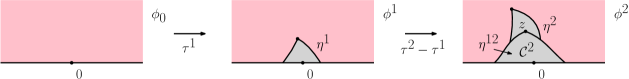
Figure 9: Figure for Proposition 5.9. The pair $(\phi^{j},\eta^{j})$ corresponds to $(\phi_{\tau_{j}},\eta_{\tau_{j}})$ translated so that the curve starts from $0$ rather than $W_{\tau_{j}}$. The curve $\eta^{12}$ is the initial segment of $\eta^{2}$.

Let $S=A_{1}+A_{2}$, then by a change of variables the law of $(\{(\phi_{t},\eta_{t})\}_{t\geq 0},A_{1},S)$ is $M\,1_{A_{1}\in[0,S]}dA_{1}\,1_{S>0}dS$. By Proposition 5.7 the law of $(A_{1},\phi^{2},\eta^{2},\tau^{2})$ is

$$C\cdot 1_{A_{1}\in[0,S]}dA_{1}\,{{\mathrm{LF}}}_{\mathbbm{H}}^{(\frac{3\gamma}{4},0),(Q-\frac{3\gamma}{4},\infty)}(d\phi^{2})\operatorname{SLE}_{\kappa}^{\tau^{2}}(d\eta^{2})1_{\tau^{2}>0}d\tau^{2},\quad S:=\mathcal{A}_{\phi^{2}}(\eta^{2}([0,\tau^{2}])).$$

Since $z$ is the point such that $\eta^{2}$ covers $S-A_{1}$ units of quantum area before hitting $z$, we conclude the law of $(z,\phi^{2},\eta^{2},\tau^{2})$ is

$$C\cdot 1_{z\in\eta^{2}([0,\tau^{2}])}\mathcal{A}_{\phi^{2}}(dz){{\mathrm{LF}}}_{\mathbbm{H}}^{(\frac{3\gamma}{4},0),(Q-\frac{3\gamma}{4},\infty)}(d\phi^{2})\operatorname{SLE}_{\kappa}^{\tau^{2}}(d\eta^{2})1_{\tau^{2}>0}d\tau^{2}.$$

By Lemma 5.10 stated below, the law of $(\phi^{2},\eta^{1},\eta^{12},z,\tau^{1})$ is

$$C\cdot\operatorname{SLE}_{\kappa}^{z}(d\eta^{12})\,\mathcal{A}_{\phi^{2}}(dz)\,{{\mathrm{LF}}}_{\mathbbm{H}}^{(\frac{3\gamma}{4},0),(Q-\frac{3\gamma}{4},\infty)}(d\phi^{2})\operatorname{SLE}_{\kappa}^{\tau^{1}}(d\eta^{1})\,1_{\tau^{1}>0}d\tau^{1}$$

where $\operatorname{SLE}_{\kappa}^{z}$ denotes forward $\operatorname{SLE}_{\kappa}$ run until the time it hits $z$. By Proposition 5.3, the law of $(\phi^{1},\eta^{1},\tau^{1},\mathcal{C}_{2},A_{2})$ is

$$C\cdot{{\mathrm{LF}}}_{\mathbbm{H}}^{(\frac{3\gamma}{4},0),(Q-\frac{3\gamma}{4},\infty)}(d\phi^{1})\operatorname{SLE}_{\kappa}^{\tau^{1}}(d\eta^{1})1_{\tau^{1}>0}d\tau^{1}P_{A_{2}}(d\mathcal{C}_{2})1_{A_{2}>0}dA_{2}.$$

By Proposition 5.7 applied to the measure $C\cdot{{\mathrm{LF}}}_{\mathbbm{H}}^{(\frac{3\gamma}{4},0),(Q-\frac{3\gamma}{4},\infty)}(d\phi^{1})\operatorname{SLE}_{\kappa}^{\tau^{1}}(d\eta^{1})1_{\tau^{1}>0}d\tau^{1}$, we conclude that the law of $(\phi_{0},\mathcal{C}_{2},A_{1},A_{2})$ is (5.7).

As a consequence of (5.7), if we sample $(\{(\phi_{t},\eta_{t})\}_{t\geq 0},A_{1},A_{2})$ from $M\times\mathrm{Unif}_{[0,\varepsilon]}(dA_{1})1_{A_{2}>0}dA_{2}$ where $\mathrm{Unif}_{[0,\varepsilon]}$ is the uniform probability measure on $[0,\varepsilon]$, then the law of $(\phi_{0},\mathcal{C}_{2},A_{1},A_{2})$ is ${{\mathrm{LF}}}_{\mathbbm{H}}^{(-\frac{\gamma}{4},0),(Q-\frac{3\gamma}{4},\infty)}(d\phi_{0})P_{A_{2}}(d\mathcal{C}_{2})\mathrm{Unif}_{[0,\varepsilon]}(dA_{1})1_{A_{2}>0}dA_{2}$. Sending $\varepsilon\to 0$ yields the desired result. ∎

Lemma 5.10.

Let $z\in\mathbbm{H}$ and consider a pair $(\eta,T)\sim 1_{E}\operatorname{SLE}_{\kappa}^{t}1_{t>0}dt$ where $E$ is the event that $z$ lies in the range of the curve. Let $\tau_{z}$ be the time $\eta$ hits $z$, let $\eta^{12}=\eta|_{[0,\tau_{z}]}$, let $T^{1}=T-\tau_{z}$ and let $\eta^{1}=f^{-1}\circ\eta(\cdot+\tau_{z})|_{[0,T^{1}]}$ where $f:\mathbbm{H}\to\mathbbm{H}\backslash\eta([0,\tau_{z}])$ is the conformal map with $f(0)=z$ and $f(w)=w+O(1)$ as $w\to\infty$. Then the law of $(\eta^{12},\eta^{1},T^{1})$ is $\operatorname{SLE}_{\kappa}^{z}\operatorname{SLE}_{\kappa}^{t^{1}}1_{t^{1}>0}dt^{1}$, where $\operatorname{SLE}_{\kappa}^{z}$ is the law of $\operatorname{SLE}_{\kappa}$ run until it hits $z$.

Proof.

From the change of variables $T^{1}=T-\tau_{z}$, the law of $T^{1}$ is $1_{t^{1}>0}dt^{1}$. Conditioned on $T^{1}$ the conditional law of $\eta^{12}$ is $\operatorname{SLE}_{\kappa}^{z}$, and by the domain Markov property, conditioned on $T^{1}$ and $\eta^{12}$ the conditional law of $\eta^{1}$ is $\operatorname{SLE}_{\kappa}^{T^{1}}$. ∎

Proof of Proposition 5.5.

By Proposition 1.6 and Definition 2.8, the area $a$ quantum cell is the quantum surface obtained by mating $(X_{t},Y_{t})_{t\geq 0}\sim\mathrm{CRT}_{\kappa}$ for quantum area $a$.

Recall $M$ from Lemma 5.6. Proposition 5.9 implies that the time-evolution of $M$ for quantum area $a$ arises from conformally welding an area $a$ quantum cell to $\phi_{0}$, and so corresponds to mating trees sampled from $\mathrm{CRT}_{\kappa}$ for quantum area $a$. Sending $a\to\infty$, we conclude that $M$ is the process of Theorem 1.7 when $n=0$ and $\delta=Q-\frac{3\gamma}{4}$. The first property of $M$ in Lemma 5.6 is the desired description of $(\phi_{\tau},\eta_{\tau})$, so we obtain Theorem 1.7 for $n=0,\delta=Q-\frac{3\gamma}{4}$. Finally, we extend to arbitrary $\delta\in\mathbbm{R}$ by Proposition 4.5. ∎

Remark 5.11.

The main difficulty in adapting our proof of Proposition 5.5 to the case $\gamma=\sqrt{2},\kappa=8$ is in proving the analog of Proposition 5.7, where ${{\mathrm{LF}}}_{\mathbbm{H}}^{(\frac{3\gamma}{4},0),(Q-\frac{3\gamma}{4},\infty)}={{\mathrm{LF}}}_{\mathbbm{H}}^{(\frac{Q}{2},0),(\frac{Q}{2},\infty)}$ has to be replaced by $\lim_{\beta\uparrow Q}\frac{1}{Q-\beta}{{\mathrm{LF}}}_{\mathbbm{H}}^{(\frac{\beta}{2},0),(\frac{Q}{2},\infty)}$. This limit is constructed in [ASY22, Section 2.5]. Our present argument does not apply since the $(M\times 1_{A>0}\,dA)$-measure of $E_{N}$ is infinite, that is, Lemma 5.8 fails for $\kappa=8$. One could try using a finite event such as $E_{N}\cap\{A<N\}$, or instead directly tackle the $\kappa=8$ variant of Proposition 5.5 by taking a $\kappa\to 8$ limit.

5.4 Proof of Theorem 1.7

In this section, we prove Theorem 1.7. The first step is to extend Proposition 5.5 to the setting where insertions are allowed but the process stops before any insertions hit the curve:

Proposition 5.12.

Theorem 1.7 holds for any stopping time $\tau$ such that a.s. $g_{\tau}(z_{j})\not\in\eta_{\tau}$ for all $j$.

Given this, we can complete the proof of Theorem 1.7.

Proof of Theorem 1.7.

Proposition 4.2 gives us a process $(\widetilde{\phi}_{t},\widetilde{\eta}_{t})_{0\leq t\leq\tau}$ such that $\widetilde{\phi}_{0}$ has law ${{\mathrm{LF}}}_{\mathbbm{H}}^{(-\frac{1}{\sqrt{\kappa}},0),(\alpha_{j},z_{j})_{j},(\delta,\infty)}$ and $(\widetilde{\phi}_{\tau},\widetilde{\eta}_{\tau})$ has law (1.2), where $\tau$ is a stopping time for $\mathcal{F}_{t}=\sigma(\widetilde{\eta}_{t})$. Let $S=\{t:g_{t}(z_{j})=W_{t}\text{ for some }j\}$. By Proposition 5.12, if $\sigma,\sigma^{\prime}$ are stopping times for $\mathcal{F}_{t}$ such that $[\sigma,\sigma^{\prime}]\cap S=\emptyset$, then on $[\sigma,\sigma^{\prime}]$ this process can alternatively be described by mating continuum random trees independent of $\mathcal{F}_{\sigma}$ until the stopping time $\sigma^{\prime}$. Since $S$ is at most finite, by continuity we conclude that the whole process $(\widetilde{\phi}_{t},\widetilde{\eta}_{t})_{0\leq t\leq\tau}$ arises from the mating-of-trees procedure described in Theorem 1.7. This completes the proof. ∎

The proof of Proposition 5.12 is identical to that of Proposition 4.5, but with different calculations which we detail below. We will show how to weight the Liouville field to introduce insertions in Lemma 5.14, then apply this to the special case of Theorem 1.7 to obtain the more general statement desired.

For Lemma 5.14 we need Lemma 4.3 and the following. Recall $G(z,w)=-\log|z-w|-\log|z-\overline{w}|$.

Lemma 5.13.

Suppose $K\subset\overline{\mathbbm{H}}$ is compact, $\mathbbm{H}\backslash K$ is simply connected and there is a conformal map $g:\mathbbm{H}\to\mathbbm{H}\backslash K$ such that $\lim_{|z|\to\infty}g(z)-z=0$. Let $\varepsilon>0$. Then for $z_{0}\in\mathbbm{H}$ such that $\operatorname{Im}z_{0}>\varepsilon$ and $u\not\in g(B_{\varepsilon}(z_{0}))$ we have $\int G(u,v)(g_{*}\theta_{\varepsilon,z_{0}})(dv)=G(u,g(z_{0}))$, where $\theta_{\varepsilon,z_{0}}$ is the uniform probability measure on $\partial B_{\varepsilon}(z_{0})$. For $x_{0}\in\partial\mathbbm{H}$ such that $g([x_{0}-\varepsilon,x_{0}+\varepsilon])\subset\mathbbm{R}$ and $u\not\in g(B_{\varepsilon}(x_{0})\cap\mathbbm{H})$ we have $\int G(u,v)(g_{*}\theta_{\varepsilon,x_{0}})(dv)=G(u,g(x_{0}))$, where $\theta_{\varepsilon,x_{0}}$ is the uniform probability measure on $\partial B_{\varepsilon}(x_{0})\cap\mathbbm{H}$.

Proof.

For the first assertion, the function $G(u,g(\cdot))$ is harmonic on $\overline{B_{\varepsilon}(z_{0})}$ because $G(u,\cdot)$ is harmonic and $g$ is conformal. Thus, by the mean value property of harmonic functions, $\int G(u,v)(g_{*}\theta_{\varepsilon,z_{0}})(dv)=\int G(u,g(v))\theta_{\varepsilon,z_{0}}(dv)=G(u,g(z_{0}))$. The second assertion is proved similarly. ∎

Now we add insertions to the Liouville field by weighting. We place constraints on the insertions so that they sum to $Q$; this allows us to work with $G(\cdot,\cdot)$ rather than the more complicated $G_{\mathbbm{H}}(\cdot,\cdot)$. Recall that $\theta_{\varepsilon,\infty}$ is the uniform probability measure on $\partial B_{1/\varepsilon}(0)\cap\mathbbm{H}$.

Lemma 5.14.

In the setting of Lemma 5.13, let $(\alpha_{j},z_{j})\in\mathbbm{R}\times\overline{\mathbbm{H}}$ and $\beta=-\sum_{j}\alpha_{j}$. Let $I=\{i:z_{i}\in\mathbbm{H}\}$ and $B=\{b:z_{b}\in\mathbbm{R}\}$. Suppose $\varepsilon>0$ satisfies $|z_{j}-z_{k}|>2\varepsilon$ for $j\neq k$, $\operatorname{Im}z_{i}>\varepsilon$ for $i\in I$, $g((z_{b}-\varepsilon,z_{b}+\varepsilon))\subset\mathbbm{R}$ for $b\in B$, and $g(-1/\varepsilon),g(1/\varepsilon)\in\mathbbm{R}$. Let $\mathbbm{H}_{\varepsilon}^{g}=\mathbbm{H}\backslash(g(\mathbbm{H}\backslash B_{1/\varepsilon}(0))\cup\bigcup_{j}g(B_{\varepsilon}(z_{j})))$ and $\theta_{\varepsilon}:=\sum_{j}\alpha_{j}\theta_{\varepsilon,z_{j}}+\beta\theta_{\varepsilon,\infty}$. For any $(\alpha,w)\in\mathbbm{R}\times\mathbbm{H}_{\varepsilon}^{g}$ and nonnegative function $F(\phi)$ depending only on $\phi|_{\mathbbm{H}_{\varepsilon}^{g}}$,

$${{\mathrm{LF}}}_{\mathbbm{H}}^{(\alpha,w),(Q-\alpha,\infty)}[\varepsilon^{-\beta^{2}+2\alpha\beta}\prod_{i\in I}\varepsilon^{\alpha_{i}^{2}/2}\prod_{b\in B}\varepsilon^{\alpha_{b}^{2}}\times e^{(g^{-1}\bullet_{\gamma}\phi,\theta_{\varepsilon})}F(\phi)]$$

$$=\prod_{i\in I}|g_{\tau}^{\prime}(z_{i})|^{2\Delta_{\alpha_{i}}}\prod_{b\in B}|g_{\tau}^{\prime}(z_{b})|^{\Delta_{2\alpha_{b}}}{{\mathrm{LF}}}_{\mathbbm{H}}^{(\alpha,w),(\alpha_{j},g(z_{j}))_{j},(\beta+Q-\alpha,\infty)}[F(\phi)].$$

Proof.

The proof of this is identical to that of Lemma 4.4; the only difference is in the computations of $Z_{\varepsilon}:=\mathbbm{E}[e^{(h,g_{*}\theta_{\varepsilon})}]$ and $e^{(g_{t}^{-1}\bullet_{\gamma}\phi,\theta_{\varepsilon})}$. To shorten notation write $\theta_{\varepsilon,j}=\theta_{\varepsilon,z_{j}}$.

To compute $Z_{\varepsilon}$ we first need $\operatorname{Var}((h,g_{*}\theta_{\varepsilon}))$. Since $\int 1\,g_{*}\theta_{\varepsilon}(dv)=0$, the law of $(h,g_{*}\theta_{\varepsilon})$ when $h\sim P_{\mathbbm{H}}$ agrees with that when $h$ is instead considered as a distribution modulo additive constant. Thus, $\operatorname{Var}((h,g_{*}\theta_{\varepsilon}))=\iint G(u,v)g_{*}\theta_{\varepsilon}(du)g_{*}\theta_{\varepsilon}(dv)$ where $G(u,v)=-\log|u-v|-\log|u-\overline{v}|$.

For $i\in I$ we have

$$\iint G(u,v)g_{*}\theta_{\varepsilon,i}(du)g_{*}\theta_{\varepsilon,i}(dv)=\int G(g(z_{i}),g(v))\theta_{\varepsilon,i}(dv)=-\log|g^{\prime}(z_{i})|+\log(2\operatorname{Im}(g(z_{i})))+\log\varepsilon,$$

where in the first equality we use Lemma 5.13 and in the second equality we use the fact that the function $f:B_{\varepsilon}(z_{i})\to\mathbbm{R}$ defined by $f(w)=-\log|g_{t}(w)-g_{t}(z_{i})|+\log|w-z_{i}|$ for $w\neq z_{i}$ and $f(z_{i})=-\log|g_{t}^{\prime}(z_{i})|$ is harmonic. Similarly, $\iint G(u,v)g_{*}\theta_{\varepsilon,b}(du)g_{*}\theta_{\varepsilon,b}(dv)=-2\log|g_{\tau}^{\prime}(z_{b})|+2\log\varepsilon$, and proceeding similarly we can compute all cross-terms. Summing gives the value of $\operatorname{Var}((h,g_{*}\theta_{\varepsilon}))$, and finally

$$Z_{\varepsilon}=e^{\frac{1}{2}{\operatorname{Var}}((h,g_{*}\theta_{\varepsilon}))}=\varepsilon^{-\beta^{2}+\sum_{i}\alpha_{i}^{2}/2+\sum_{b}\alpha_{b}^{2}}\prod_{i\in I}|g^{\prime}(z_{i})|^{-\alpha_{i}^{2}/2}\prod_{b\in B}|g^{\prime}(z_{b})|^{-\alpha_{b}^{2}}C_{\gamma}^{(\alpha_{j},g(z_{j}))_{j},(\beta,\infty)}.$$

Next, by Lemmas 4.3 and 5.13 we have $(G(\cdot,w),g_{*}\theta_{\varepsilon})=-2\beta\log\varepsilon+\sum_{j}\alpha_{j}G(z_{j},w)$, so with $\phi=h+\alpha G(\cdot,w)+c$, we have

$$e^{(g^{-1}\bullet_{\gamma}\phi,\theta_{\varepsilon})}=\varepsilon^{2\alpha\beta}\frac{C_{\gamma}^{(\alpha,w),(\alpha_{j},g(z_{j}))_{j},(\delta,\infty)}}{C_{\gamma}^{(\alpha_{j},g(z_{j}))_{j},(\beta,\infty)}}e^{(h,g_{*}\theta_{\varepsilon})}.$$

The rest of the argument is identical to that of Lemma 4.4. ∎

Proof of Proposition 5.12.

By Proposition 5.5, Theorem 1.7 holds for $n=0,\delta=Q+\frac{\gamma}{4}$. Applying the argument of Proposition 4.5 with Lemma 5.14 as input, we obtain the $n\geq 0$ case when the insertions $(\alpha_{j},z_{j})_{j}$ and $(\delta,\infty)$ satisfy $-\frac{1}{\sqrt{\kappa}}+\sum_{j}\alpha_{j}+\delta=Q$. We were able to use Lemma 5.14 because of the condition $g_{\tau}(z_{j})\not\in\eta_{\tau}$. A final application of Proposition 4.5 removes this constraint. ∎

6 The $\kappa\in(4,8)$ LCFT zipper

In this section we prove Theorem 1.5.

[DMS21, Theorem 6.9] says that when a particular GFF variant is cut by a forward $\operatorname{SLE}_{\kappa}$ with $\kappa\in(4,8)$, the connected components in the complement of the curve are a pair of independent forested lines. In fact, their argument (together with the addition of a constant $\mathbf{c}\sim dc$) proves the following stronger result.

Proposition 6.1.

Theorem 1.5 holds for $n=0$ and $\delta=Q+\frac{\gamma}{4}$.

Proof.

The setup of [DMS21, Theorem 6.9] starts with a field $h_{0}=h+\frac{\gamma}{2}\log|\cdot|$ where $h\sim P_{\mathbbm{H}}$, and uses Proposition 4.1 to get a field and curve $h_{t},\eta_{t}$ where the law of $\eta_{t}$ is reverse $\operatorname{SLE}_{\kappa}$ run for time $t$ and the conditional law of $h_{t}$ given $\eta_{t}$ is $\widetilde{h}+\frac{\gamma}{2}\log|\cdot-\eta_{t}(0)|$ where $\widetilde{h}$ is a Neumann GFF with a normalization that depends on $\eta_{t}$.

[DMS21, Theorem 6.9] states that the bounded connected components in $\mathbbm{H}\backslash\eta_{t}$ are a countable collection of quantum surfaces arising from a Poisson point process of LQG disks, and by the definition of forested line in [DMS21] these quantum surfaces come from a pair of independent forested lines. In fact, their argument not only proves independence of these quantum surfaces, but also implicitly proves their independence from $h_{0}$; this gives the independence of $h_{0}$ and the forested lines. The fact that $(h_{t},\eta_{t})$ is obtained by mating the forested lines as in Proposition 1.4 follows from local absolute continuity with respect to that setting.

Finally, if we add a constant $\mathbf{c}$ chosen from Lebesgue measure on $\mathbbm{R}$, both $h_{0}$ and $h_{t}(\cdot+\eta_{t}(0))$ have the marginal law of the Liouville field ${{\mathrm{LF}}}_{\mathbbm{H}}^{(-\frac{\gamma}{4},0),(Q+\frac{\gamma}{4},\infty)}$. Since forested lines are scale-invariant in law (i.e. are invariant in law under adding a constant to the field), this completes the proof of Theorem 1.5 when $n=0,\delta=Q+\frac{\gamma}{4}$ and $\tau=t$ is a deterministic time. The result where $\tau\in\{2^{-m}k:k,m\in\mathbbm{Z}\}$ a.s. is then immediate, and a limit gives the result for general $\tau$ (this is the same argument proving the strong Markov property of Brownian motion from the Markov property). ∎

Proof of Theorem 1.5.

Starting with Proposition 6.1, Proposition 4.5 gives Theorem 1.5 for $n=0$. Then the arguments of Sections 5.4 yield the full Theorem 1.5. ∎

7 The boundary BPZ equation for Liouville conformal field theory

In this section we use the LCFT quantum zipper to prove the boundary BPZ equations stated in Theorem 1.10. Let $m,n\geq 0$. Let $(\alpha_{j},z_{j})\in\mathbbm{R}\times\mathbbm{H}$ for $j\leq m$ and assume $z_{1},\dots,z_{m}$ are distinct. Let $-\infty=x_{0}<x_{1}<\dots<x_{n}<x_{n+1}=+\infty$, let $\beta_{1},\dots,\beta_{n}\in\mathbbm{R}$ and let $\delta\in\mathbbm{R}$. Let $\beta_{*}\in\{-\frac{\gamma}{2},-\frac{2}{\gamma}\}$ and recall the LCFT correlation function $F_{\beta_{*}}(w,(z_{j})_{j},(x_{k})_{k})$ defined in (1.5).

In Section 7.1 we prove the BPZ equation holds for $\beta_{*}=-\frac{2}{\gamma}$, in Section 7.2 we handle the case $\beta_{*}=-\frac{\gamma}{2}$ and $\gamma\in(0,\sqrt{2})$ and in Section 7.3 we settle the case $\beta_{*}=-\frac{\gamma}{2}$ and $\gamma\in(\sqrt{2},2)$ case. These sections use the coupling of LCFT with $\operatorname{SLE}_{\kappa}$ for $\kappa\in(0,4],(8,\infty),(4,8)$ respectively.

Proof of Theorem 1.10.

For $\gamma\in(0,2]$ the $\beta_{*}=-\frac{2}{\gamma}$ BPZ equation is shown in Lemma 7.2. For $\gamma\in(0,\sqrt{2})$ and $\beta_{*}=-\frac{\gamma}{2}$ it is shown in Lemma 7.5, and for $\gamma\in(\sqrt{2},2)$ and $\beta_{*}=-\frac{\gamma}{2}$ see Lemma 7.8. Finally, when $\gamma=2$ we have $-\frac{\gamma}{2}=-\frac{2}{\gamma}$ so the $\beta_{*}=-\frac{\gamma}{2}$ BPZ equation has already been settled by the first case. ∎

7.1 Case: $\beta_{*}=-\frac{2}{\gamma}$

Let $\kappa\leq 4$ and $\gamma=\sqrt{\kappa}$. Consider reverse $\operatorname{SLE}_{\kappa}$ where the driving function $W_{t}$ is given by $W_{0}=w$ and $dW_{t}=\sqrt{\kappa}dB_{t}$. Let $(\eta_{t})_{t\geq 0}$ be the family of curves and $g_{t}$ the corresponding Loewner maps, and let $T\leq\infty$ be the first time $t$ that $g_{t}(x_{k})\in\eta_{t}$ for some $k$. For $t<T$ define

$$M_{t}=\prod_{j}|g_{t}^{\prime}(z_{j})|^{2\Delta_{\alpha_{j}}}\prod_{k}|g_{t}^{\prime}(x_{k})|^{\Delta_{\beta_{k}}}F_{-\frac{2}{\gamma}}(W_{t},(g_{t}(z_{j}))_{j},(g_{t}(x_{k}))_{k}).$$ (7.1)

Lemma 7.1.

$M_{t}$ is a local martingale.

Proof.

Let $\overline{F}_{-\frac{2}{\gamma}}(w,(z_{j})_{j},(x_{k})_{k})<\infty$ be defined via (1.5) except with the integrand replaced by its absolute value, and let $\overline{M}_{t}=\prod_{j}|g_{t}^{\prime}(z_{j})|^{2\Delta_{\alpha_{j}}}\prod_{k}|g_{t}^{\prime}(x_{k})|^{\Delta_{\beta_{k}}}\overline{F}_{-\frac{2}{\gamma}}(w,(z_{j})_{j},(x_{k})_{k})$, so $\overline{M}_{t}\geq|M_{t}|$. For $N>0$ let $T_{N}=T\wedge\inf\{t:\overline{M}_{t}\geq N\}$. Since $t\mapsto\overline{M}_{t}$ is continuous on $[0,T)$ we have $\lim_{N\to\infty}T_{N}=T$ almost surely. Thus we are done once we show $M_{t}$ stopped at $T_{N}$ is a martingale.

It suffices to show that for stopping times $\tau_{1}\leq\tau_{2}\leq T_{N}$ we have $\mathbbm{E}[M_{\tau_{2}}\mid\eta_{\tau_{1}}]=M_{\tau_{1}}$. Instead, to simplify notation, we show that if $\tau\leq T_{N}$ is a stopping time then $\mathbbm{E}[M_{\tau}]=M_{0}$; the proof of the desired claim is identical.

Sample $\phi_{0}\sim{{\mathrm{LF}}}_{\mathbbm{H}}^{(\frac{\beta_{*}}{2},w),(\alpha_{j},z_{j})_{j},(\frac{\beta_{k}}{2},x_{k})_{k},(\frac{\delta}{2},\infty)}$, and define $(\phi_{t},\eta_{t})$ by conformally welding the boundary arcs to the left and right of $w$ as in Theorem 1.1. Let $A_{t}=\mathcal{A}_{\phi_{t}}(\mathbbm{H})$, let $L_{k,t}=\mathcal{L}_{\phi_{t}}(g_{t}(I_{k}))$ for $k\neq k_{*}$, and let $L_{t}=\mathcal{L}_{\phi_{t}}((g_{t}(x_{k_{*}}),W_{t}))$ and $R_{t}=\mathcal{L}_{\phi_{t}}((W_{t},g_{t}(x_{k_{*}+1}))$. Since the conformal welding does not affect the quantum area nor quantum lengths of boundary segments not adjacent to $w$, the processes $A_{t}$ and $L_{k,t}$ are constant. Moreover, the conformal welding identifies segments of equal quantum length, so $L_{t}-R_{t}=L_{0}-R_{0}$ for all $t$. Thus, $G_{t}=\exp(-A_{t}-\sum_{k\neq k_{*}}\mu_{k}L_{k,t}-\mu_{L}(L_{t}-R_{t}))$ is constant as $t$ varies. Consequently, writing $\mathbbm{E}$ to denote expectation with respect to $\operatorname{rSLE}_{\kappa}^{\tau}$ and using Theorem 1.1, we have

$$M_{0} ={{\mathrm{LF}}}_{\mathbbm{H}}^{(-\frac{1}{\sqrt{\kappa}},w),(\alpha_{j},z_{j})_{j},(\frac{\beta_{k}}{2},x_{k})_{k},(\frac{\delta}{2},\infty)}[G_{0}]$$ (7.2)

$$=\mathbbm{E}[\prod_{j}|g_{\tau}^{\prime}(z_{j})|^{2\Delta_{\alpha_{j}}}\prod_{k}|g_{\tau}^{\prime}(x_{k})|^{\Delta_{\beta_{k}}}{{\mathrm{LF}}}_{\mathbbm{H}}^{(-\frac{1}{\sqrt{\kappa}},W_{\tau}),(\alpha_{j},g_{\tau}(z_{j}))_{j},(\frac{\beta_{k}}{2},g_{\tau}(x_{k}))_{k},(\frac{\delta}{2},\infty)}[G_{\tau}]]=\mathbbm{E}[M_{\tau}].$$

Here, the integrals converge absolutely by the definition of $T_{N}$. This completes the proof. ∎

If we assume that $F_{-\frac{2}{\gamma}}$ is smooth, then setting the drift term of $dM_{t}$ to zero immediately gives Theorem 1.10 for $\beta_{*}=-\frac{2}{\gamma}$. Since we do not have smoothness a priori, we only know $F_{-\frac{2}{\gamma}}$ is a weak solution to the BPZ equation. A hypoellipticity argument originally due to [Dub15, Lemma 5] shows that weak solutions are also strong solutions; we instead follow [PW19, Lemma 4.4, Proposition 2.6] which is closer to our setting.

Lemma 7.2.

Theorem 1.10 holds for $\beta_{*}=-\frac{2}{\gamma}$.

Proof.

Consider the diffusion $X_{t}=(W_{t},(g_{t}(z_{j}))_{j},(g_{t}(x_{k}))_{k},(|g_{t}^{\prime}(z_{j})|)_{j},(|g_{t}^{\prime}(x_{k})|)_{k})$ where $W_{t}$ and $g_{t}$ are defined above (7.1). For each $t$ we have $X_{t}\in\mathbbm{R}\times\mathbbm{H}^{m}\times\mathbbm{R}^{n}\times\mathbbm{R}^{m}\times\mathbbm{R}^{n}$. We denote the coordinates of an element of $\mathbbm{R}\times\mathbbm{H}^{m}\times\mathbbm{R}^{n}\times\mathbbm{R}^{m}\times\mathbbm{R}^{n}$ by $(\mathbf{w},(\mathbf{z}_{j})_{j},(\mathbf{x}_{k})_{k},(\mathbf{a}_{j})_{j},(\mathbf{b}_{k})_{k})$; with this notation, since $dg_{t}(z)=-\frac{2}{g_{t}(z)-W_{t}}dt$ and $d|g_{t}^{\prime}(z)|=\operatorname{Re}\frac{2|g_{t}^{\prime}(z)|}{(g_{t}(z)-W_{t})^{2}}dt$, the infinitesimal generator $A$ of $X_{t}$ is

$$A=\frac{\kappa}{2}\partial_{\mathbf{w}}^{2}-\sum_{j}(\frac{2}{\mathbf{z}_{j}-\mathbf{w}}\partial_{\mathbf{z}_{j}}+\frac{2}{\overline{\mathbf{z}}_{j}-\mathbf{w}}\partial_{\overline{\mathbf{z}}_{j}})-\sum_{k}\frac{2}{\mathbf{x}_{k}-\mathbf{w}}\partial_{\mathbf{x}_{k}}+\sum_{j}\operatorname{Re}\frac{2\mathbf{a}_{j}}{(\mathbf{z}_{j}-\mathbf{w})^{2}}\partial_{\mathbf{a}_{j}}+\sum_{j}\frac{2\mathbf{b}_{k}}{(\mathbf{x}_{k}-\mathbf{w})^{2}}\partial_{\mathbf{b}_{k}}.$$

Let $F(\mathbf{w},(\mathbf{z}_{j})_{j},(\mathbf{x}_{k})_{k},(\mathbf{a}_{j})_{j},\mathbf{b}_{k})_{k})=\prod_{j}\mathbf{a}_{j}^{2\Delta_{\alpha_{j}}}\prod_{k}\mathbf{b}_{k}^{\Delta_{\beta_{k}}}F_{-\frac{2}{\gamma}}(\mathbf{w},(\mathbf{z}_{j})_{j},(\mathbf{x}_{k})_{k})$. Since $M_{t}$ is a local martingale (Lemma 7.1), $F$ is a weak solution to $AF=0$. The product rule then yields

$$0=A\Big{(}\prod_{j}\mathbf{a}_{j}^{2\Delta_{\alpha_{j}}}\prod_{k}\mathbf{b}_{k}^{\Delta_{\beta_{k}}}F_{-\frac{2}{\gamma}}(\mathbf{w},(\mathbf{z}_{j})_{j},(\mathbf{x}_{k})_{k})\Big{)}=\prod_{j}\mathbf{a}_{j}^{2\Delta_{\alpha_{j}}}\prod_{k}\mathbf{b}_{k}^{\Delta_{\beta_{k}}}\mathcal{D}F_{-\frac{2}{\gamma}}(\mathbf{w},(\mathbf{z}_{j})_{j},(\mathbf{x}_{k})_{k})$$

where $\mathcal{D}$ is the differential operator on $\mathbbm{R}\times\mathbbm{H}^{m}\times\mathbbm{R}^{n}$ given by

$$\mathcal{D}:=\frac{\kappa}{2}\partial_{\mathbf{w}}^{2}-\sum_{j}(\frac{2}{\mathbf{z}_{j}-\mathbf{w}}\partial_{\mathbf{z}_{j}}+\frac{2}{\overline{\mathbf{z}}_{j}-\mathbf{w}}\partial_{\overline{\mathbf{z}}_{j}})-\sum_{k}\frac{2}{\mathbf{x}_{k}-\mathbf{w}}\partial_{\mathbf{x}_{k}}+\sum_{j}\operatorname{Re}\frac{4\Delta_{\alpha_{j}}}{(\mathbf{z}_{j}-\mathbf{w})^{2}}+\sum_{j}\frac{2\Delta_{\beta_{k}}}{(\mathbf{x}_{k}-\mathbf{w})^{2}}.$$

We conclude that $\mathcal{D}F_{-\frac{2}{\gamma}}=0$ in the distributional sense.

The operator $\mathcal{D}$ is called hypoelliptic if the weak solutions of $\mathcal{D}F=0$ are smooth. Hörmander’s condition gives a criterion for hypoellipticity which is applicable to $\mathcal{D}$; this is explained in [PW19, Proposition 2.6] for a similar differential operator but the argument carries over directly. Since $\mathcal{D}$ is hypoelliptic, $F_{-\frac{2}{\gamma}}$ is smooth and $\mathcal{D}F_{-\frac{2}{\gamma}}=0$ is the desired BPZ equation. ∎

7.2 Case: $\gamma\in(0,\sqrt{2})$ and $\beta_{*}=-\frac{\gamma}{2}$

For $\kappa>4$, recall that $\mathrm{CRT}_{\kappa}$ is the joint law of the correlated Brownian motion $(X_{s},Y_{s})_{s\geq 0}$ defined by $\operatorname{Var}(X_{s})=\operatorname{Var}(Y_{s})=\mathbbm{a}^{2}s$ and $\operatorname{Cov}(X_{s},Y_{s})=-\mathbbm{a}^{2}\cos(\frac{4\pi}{\kappa})s$, where $\mathbbm{a}^{2}=2/\sin(\frac{4\pi}{\kappa})$. The key to the BPZ equation is the following martingale which explains the coupling (1.3) between $\mu_{L},\mu_{R}$.

Lemma 7.3.

For $\kappa>4$, let $\theta=\frac{4\pi}{\kappa}$ and $x\in\mathbbm{C}$. Set $\mu_{L}=\sqrt{1/\sin\theta}\cos x$ and $\mu_{R}=\sqrt{1/\sin\theta}\cos(x+\theta)$. Then the process $e^{-s-\mu_{L}X_{s}-\mu_{R}Y_{s}}$ is a martingale.

Proof.

We need the trigonometric identity

$$\cos^{2}x+\cos^{2}(x+\theta)-2\cos x\cos(x+\theta)\cos\theta=\sin^{2}\theta.$$ (7.3)

To see that this holds, we compute

$$2\cos x\cos(x+\theta)\cos\theta=(\cos(2x+\theta)+\cos(\theta))\cos\theta$$

$$=\frac{1}{2}\cos(2(x+\theta))+\frac{1}{2}\cos 2x+1-\sin^{2}\theta=\cos^{2}(x+\theta)+\cos^{2}x-\sin^{2}\theta,$$

where the first equality uses the product-to-sum formula, the second uses the product-to-sum formula and $\sin^{2}+\cos^{2}=1$, and the last uses the double-angle formula. Now, using (7.3) gives

$$\mathbbm{E}[e^{-s-\mu_{L}L_{s}-\mu_{R}R_{s}}]=\exp(-s+\frac{1}{2}(\mu_{L}^{2}+\mu_{R}^{2}-2\mu_{L}\mu_{R}\cos\theta)\mathbbm{a}^{2}s)=\exp(-s+\frac{1}{2\sin\theta}\cdot\sin^{2}\theta\cdot\mathbbm{a}^{2}s)=1.$$

This and the strong Markov property of Brownian motion imply that $e^{-s-\mu_{L}L_{s}-\mu_{R}R_{s}}$ is a martingale. ∎

Consider reverse $\operatorname{SLE}_{\kappa}$ where the driving function $W_{t}$ is given by $W_{0}=w$ and $dW_{t}=\sqrt{\kappa}dB_{t}$. Let $(\eta_{t})_{t\geq 0}$ be the family of curves, and let $T\leq\infty$ be the first time $t$ that $g_{t}(x_{k})\in\eta_{t}$ for some $k$. For $t<T$ define

$$M_{t}=\prod_{j}|g_{t}^{\prime}(z_{j})|^{2\Delta_{\alpha_{j}}}\prod_{k}|g_{t}^{\prime}(x_{k})|^{\Delta_{\beta_{k}}}F_{-\frac{\gamma}{2}}(W_{t},(g_{t}(z_{j}))_{j},(g_{t}(x_{k}))_{k}).$$

Lemma 7.4.

In the case $\kappa>8$, $M_{t}$ is a local martingale.

Proof.

For $N>0$ define the stopping time $T_{N}$ as in Lemma 7.1, then it suffices to show that $M_{t}$ stopped at $T_{N}$ is a martingale. As before, we need to show that for stopping times $\tau_{1}\leq\tau_{2}\leq T_{N}$ we have $\mathbbm{E}[M_{\tau_{2}}\mid\eta_{\tau_{1}}]=M_{\tau_{1}}$. We instead show that if $\tau\leq T_{N}$ is a stopping time then $\mathbbm{E}[M_{\tau}]=M_{0}$; the former is proved identically. Similarly, to lighten notation we assume that $\mu_{k}=0$ for all $k\neq k_{*}$.

Sample $(\phi_{0},(X_{\cdot},Y_{\cdot})_{[0,\infty)})\sim{{\mathrm{LF}}}_{\mathbbm{H}}^{(\frac{\beta_{*}}{2},w),(\alpha_{j},z_{j})_{j},(\frac{\beta_{k}}{2},x_{k}),(\frac{\delta}{2},\infty)}\times\mathrm{CRT}_{\kappa}$, attach the continuum random trees to $(-\infty,w)$ and $(w,\infty)$, and define $(\phi_{t},\eta_{t})$ as in Theorem 1.7. For each $t\leq\tau$ let $s(t):=\mathcal{A}_{\phi_{t}}(\eta_{t}((0,t)))$, i.e. $(\phi_{t},\eta_{t})$ arises from mating the trees $(X_{\cdot},Y_{\cdot})_{[0,\infty)}$ for time $s$. Let $\sigma=s(\tau)$. The time $\sigma$ is a stopping time for the filtration $\widetilde{\mathcal{F}}_{s}=\sigma(\phi_{0},(X_{\cdot},Y_{\cdot})_{[0,s]})$, since for $s=s(t)$ the pair $(\phi_{t},\eta_{t})$ is obtained from $(\phi_{0},(X_{\cdot},Y_{\cdot})_{[0,s]})$ by mating the trees for time $s$.

Let $A_{t}=\mathcal{A}_{\phi_{t}}(\mathbbm{H})$, $L_{t}=\mathcal{L}_{\phi_{t}}((g_{t}(x_{k_{*}}),W_{t}))$ and $R_{t}=\mathcal{L}_{\phi_{t}}((W_{t},g_{t}(x_{k_{*}+1})))$. Let $G_{t}=e^{-A_{t}-\mu_{L}L_{t}-\mu_{R}R_{t}}$. We claim that

$$\mathbbm{E}[G_{\tau}\mid\phi_{0}]=G_{0}.$$

Indeed, the mating-of-trees procedure gives $A_{\tau}-A_{0}=\sigma,L_{\tau}-L_{0}=X_{\sigma}$ and $R_{\tau}-R_{0}=Y_{\sigma}$ (see Figure 10), and $\sigma$ is a stopping time for $\widetilde{\mathcal{F}}_{s}$ given $\phi_{0}$. Then $\mathbbm{E}[G_{\tau}\mid\phi_{0}]=G_{0}$ follows from Lemma 7.3.

Consequently, by Theorem 1.7, Equation (7.2) holds in this setting, so $\mathbbm{E}[M_{\tau}]=M_{0}$ as desired. ∎

Figure 10: Let $\kappa>8$. If $s=s(t)$ is such that $(\phi_{t},\eta_{t})$ arises from mating the trees for time $s$, then the changes in boundary arc lengths are $(L_{t}-L_{0},R_{t}-R_{0})=(X_{s},Y_{s})$.

Lemma 7.5.

Theorem 1.10 holds for $\beta_{*}=-\frac{\gamma}{2}$ and $\gamma\in(0,\sqrt{2})$.

Proof.

Given Lemma 7.4 the argument of Lemma 7.2 implies the result. ∎

7.3 Case: $\gamma\in(\sqrt{2},2)$ and $\beta_{*}=-\frac{\gamma}{2}$

In this section we prove Theorem 1.10 for $\gamma\in(\sqrt{2},2)$ and $\beta_{*}=-\frac{\gamma}{2}$.

We set $\kappa=\frac{16}{\gamma^{2}}\in(4,8)$. In this regime, $\operatorname{SLE}_{\kappa}$ is self-hitting but not space-filling. There is a variant called space-filling $\operatorname{SLE}_{\kappa}$ [MS17] with the property that if $\eta^{\mathrm{SF}}$ is space-filling $\operatorname{SLE}_{\kappa}$ in $(\mathbbm{H},0,\infty)$, and $T$ is the set of times $t$ that $\eta^{\mathrm{SF}}(t)$ is on the boundary of the unbounded connected component of $\mathbbm{H}\backslash\eta^{\mathrm{SF}}([0,t])$, then the ordered collection of points $\{\eta^{\mathrm{SF}}(t):t\in T\}$ has the law of ordinary $\operatorname{SLE}_{\kappa}$ in $(\mathbbm{H},0,\infty)$. This gives a coupling of space-filling $\operatorname{SLE}_{\kappa}$ and ordinary $\operatorname{SLE}_{\kappa}$.

The weight $(2-\frac{\gamma^{2}}{2})$ quantum wedge is thin since $2-\frac{\gamma^{2}}{2}\in(0,\frac{\gamma^{2}}{2})$ for $\gamma\in(\sqrt{2},2)$. We define space-filling $\operatorname{SLE}_{\kappa}$ on the thin quantum wedge to be the concatenation of independent space-filling $\operatorname{SLE}_{\kappa}$ curves between the marked points in each connected component, and similarly define ordinary $\operatorname{SLE}_{\kappa}$ on the thin quantum wedge. We state the mating of trees theorem for this range of $\gamma$, see Figure 11.

Proposition 7.6 ([DMS21, Theorem 1.9]).

Let $\kappa\in(4,8)$ and $\gamma=\frac{4}{\sqrt{\kappa}}$. Sample a weight $(2-\frac{\gamma^{2}}{2})$ quantum wedge decorated by an independent space-filling $\operatorname{SLE}_{\kappa}$ $\eta^{\mathrm{SF}}$. Parametrize $\eta^{\mathrm{SF}}$ by quantum area. On the counterclockwise (resp. clockwise) boundary arc of $\eta^{\mathrm{SF}}([0,s])$ from $0$ to $\eta(s)$, let $X_{s}^{-}$ and $X_{s}^{+}$ (resp. $Y_{s}^{-}$ and $Y_{s}^{+}$) be the quantum lengths of the boundary segments lying in the quantum wedge’s boundary and bulk respectively. Then the law of $(X_{s},Y_{s}):=(X_{s}^{+}-X_{s}^{-},Y_{s}^{+}-Y_{s}^{-})$ is $\mathrm{CRT}_{\kappa}$. Moreover, the curve-decorated quantum wedge is measurable with respect to $(X_{s},Y_{s})_{s\geq 0}$.

Figure 11: Let $\kappa\in(4,8)$. Left: A pair of correlated continuum random trees described by $(X_{s},Y_{s})_{s\geq 0}$. Right: Mating the trees gives a weight $(2-\frac{\gamma^{2}}{2})$ quantum wedge decorated by an independent space-filling $\operatorname{SLE}_{\kappa}$ curve. Middle: The trees have been mated until the quantum area is $s$. We write $X_{s}^{-},X_{s}^{+},Y_{s}^{-},Y_{s}^{+}$ for the quantum lengths of the four labelled boundary arcs.

Figure 12: Let $\kappa\in(4,8)$. Left: A pair of independent forested lines. Middle: The forested lines have been mated for some amount of time. Right: The pair of forested lines can be coupled with a sample from $\mathrm{CRT}_{\kappa}$ such that the middle picture is obtained by mating continuum random trees, then replacing the space-filling $\operatorname{SLE}_{\kappa}$ with its coupled non-space-filling $\operatorname{SLE}_{\kappa}$.

As before, consider reverse $\operatorname{SLE}_{\kappa}$ where the driving function $W_{t}$ is given by $W_{0}=w$ and $dW_{t}=\sqrt{\kappa}dB_{t}$. Let $(\eta_{t})_{t\geq 0}$ be the family of curves, and let $T\leq\infty$ be the first time $t$ that $g_{t}(x_{k})\in\eta_{t}$ for some $k$. For $t<T$ define

$$M_{t}=\prod_{j}|g_{t}^{\prime}(z_{j})|^{2\Delta_{\alpha_{j}}}\prod_{k}|g_{t}^{\prime}(x_{k})|^{\Delta_{\beta_{k}}}F_{-\frac{\gamma}{2}}(W_{t},(g_{t}(z_{j}))_{j},(g_{t}(x_{k}))_{k}).$$

Lemma 7.7.

In the case $\kappa\in(4,8)$, $M_{t}$ is a local martingale.

Proof.

For $N>0$ we define the stopping time $T_{N}$ as in Lemma 7.1. As in Lemma 7.4 we assume that $\mu_{k}=0$ for all $k\neq k_{*}$, and we prove that for a stopping time $\tau\leq T_{N}$ we have $\mathbbm{E}[M_{\tau}]=M_{0}$; the full result follows from the same argument.

Sample $(\phi_{0},(X_{\cdot},Y_{\cdot})_{[0,\infty)})\sim{{\mathrm{LF}}}_{\mathbbm{H}}^{(-\frac{1}{\sqrt{\kappa}},w),(\alpha_{j},z_{j})_{j},(\frac{\beta_{k}}{2},x_{k}),(\frac{\delta}{2},\infty)}\times\mathrm{CRT}_{\kappa}$, consider the space-filling-$\operatorname{SLE}_{\kappa}$-decorated thin quantum wedge obtained by mating $(X_{\cdot},Y_{\cdot})_{[0,\infty)}$, and let $(F_{L},F_{R})$ be the pair of forested lines obtained by cutting this quantum wedge by the coupled ordinary $\operatorname{SLE}_{\kappa}$ curve. By definition the law of $(\phi_{0},(F_{L},F_{R}))$ is ${{\mathrm{LF}}}_{\mathbbm{H}}^{(-\frac{1}{\sqrt{\kappa}},w),(\alpha_{j},z_{j})_{j},(\frac{\beta_{k}}{2},x_{k}),(\frac{\delta}{2},\infty)}\times\mathrm{FL}_{\kappa}$, see Figure 12.

Let $(\phi_{t},\eta_{t})$ be the field and curve obtained from $(\phi_{0},(F_{L},F_{R}))$ by mating the forested lines as in Theorem 1.5. By our construction, $(\phi_{t},\eta_{t})$ arises from mating the trees $(X_{\cdot},Y_{\cdot})_{[0,\infty)}$ for some time $s=s(t)$ to get $(\phi_{t},\eta^{\mathrm{SF}}_{t})$ where $\eta^{\mathrm{SF}}_{t}$ is a space-filling curve, then replacing $\eta^{\mathrm{SF}}_{t}$ with its coupled non-space-filling curve $\eta_{t}$. Consequently, $\sigma=s(\tau)$ is a stopping time for $\widetilde{\mathcal{F}}_{s}=\sigma(\phi_{0},(X_{\cdot},Y_{\cdot})_{[0,s]})$.

Let $A_{t}=\mathcal{A}_{\phi_{t}}(\mathbbm{H})$, $L_{t}=\mathcal{L}_{\phi_{t}}((g_{t}(x_{k_{*}}),W_{t}))$ and $R_{t}=\mathcal{L}_{\phi_{t}}((W_{t},g_{t}(x_{k_{*}+1})))$. Let $G_{t}=e^{-A_{t}-\mu_{L}L_{t}-\mu_{R}R_{t}}$. As in the proof of Lemma 7.4, the martingale of Lemma 7.3 gives $\mathbbm{E}[G_{\tau}\mid\phi_{0}]=G_{0}$. Consequently, by Theorem 1.7, Equation (7.2) holds in this setting, so $\mathbbm{E}[M_{\tau}]=M_{0}$. We are done. ∎

Lemma 7.8.

Theorem 1.10 holds for $\beta_{*}=-\frac{\gamma}{2}$ and $\gamma\in(\sqrt{2},2)$.

Proof.

Given Lemma 7.7 the argument of Lemma 7.2 implies the result. ∎

References

- [AHS22] M. Ang, N. Holden, and X. Sun. Integrability of SLE via conformal welding of random surfaces. Communications on Pure and Applied Mathematics, to appear, 2022.
- [AHS23] M. Ang, N. Holden, and X. Sun. Conformal welding of quantum disks. Electronic Journal of Probability, 28:1–50, 2023.
- [Ale19] O. Alekseev. Stochastic interface dynamics in the Hele-Shaw cell. Physical Review E, 100(1):012130, 2019.
- [ARS22] M. Ang, G. Remy, and X. Sun. FZZ formula of boundary Liouville CFT via conformal welding. Journal of the European Mathematical Society, to appear, 2022.
- [ARSZ] M. Ang, G. Remy, X. Sun, and T. Zhu. Derivation of all structure constants for boundary Liouville CFT. Forthcoming.
- [AS21] M. Ang and X. Sun. Integrability of the conformal loop ensemble. ArXiv e-prints, 2021, 2107.01788.
- [ASY22] M. Ang, X. Sun, and P. Yu. Quantum triangles and imaginary geometry flow lines. ArXiv e-prints, 2022, 2211.04580.
- [BB03] M. Bauer and D. Bernard. Conformal field theories of stochastic Loewner evolutions. Communications in Mathematical Physics, 239(3):493–521, 2003.
- [BBK05] M. Bauer, D. Bernard, and K. Kytölä. Multiple Schramm-Loewner evolutions and statistical mechanics martingales. J. Stat. Phys., 120(5-6):1125–1163, 2005. MR2187598 (2007d:82032)
- [BPZ84] A. A. Belavin, A. M. Polyakov, and A. B. Zamolodchikov. Infinite Conformal Symmetry in Two-Dimensional Quantum Field Theory. Nucl. Phys., B241:333–380, 1984.
- [CDCH+14] D. Chelkak, H. Duminil-Copin, C. Hongler, A. Kemppainen, and S. Smirnov. Convergence of Ising interfaces to Schramm’s SLE curves. Comptes Rendus Mathematique, 352(2):157–161, 2014.
- [Cer22] B. Cerclé. Three-point correlation functions in the toda theory I: Reflection coefficients. ArXiv e-prints, 2022, 2206.06902.
- [DKRV16] F. David, A. Kupiainen, R. Rhodes, and V. Vargas. Liouville quantum gravity on the Riemann sphere. Comm. Math. Phys., 342(3):869–907, 2016, 1410.7318. MR3465434
- [DMS21] B. Duplantier, J. R. Miller, and S. Sheffield. Liouville quantum gravity as a mating of trees. Astérisque, 427, 2021.
- [DRSV14] B. Duplantier, R. Rhodes, S. Sheffield, and V. Vargas. Critical Gaussian multiplicative chaos: convergence of the derivative martingale. Ann. Probab., 42(5):1769–1808, 2014, 1206.1671. MR3262492
- [DRV16] F. David, R. Rhodes, and V. Vargas. Liouville quantum gravity on complex tori. J. Math. Phys., 57(2):022302, 25, 2016, 1504.00625. MR3450564
- [DS11] B. Duplantier and S. Sheffield. Liouville quantum gravity and KPZ. Invent. Math., 185(2):333–393, 2011, 1206.0212. MR2819163 (2012f:81251)
- [Dub15] J. Dubédat. SLE and Virasoro representations: localization. Communications in Mathematical Physics, 336(2):695–760, 2015.
- [Fuk17] Y. Fukusumi. Time reversing procedure of SLE and 2d gravity. arXiv preprint arXiv:1710.08670, 2017.
- [FZZ00] V. Fateev, A. B. Zamolodchikov, and A. B. Zamolodchikov. Boundary Liouville field theory. 1. Boundary state and boundary two point function. 1 2000, hep-th/0001012.
- [GHMS17] E. Gwynne, N. Holden, J. Miller, and X. Sun. Brownian motion correlation in the peanosphere for . Ann. Inst. Henri Poincaré Probab. Stat., 53(4):1866–1889, 2017, 1510.04687. MR3729638
- [GKRV21] C. Guillarmou, A. Kupiainen, R. Rhodes, and V. Vargas. Segal’s axioms and bootstrap for Liouville Theory. ArXiv e-prints, 2021, 2112.14859.
- [GKRV22] C. Guillarmou, A. Kupiainen, R. Rhodes, and V. Vargas. Conformal bootstrap in Liouville Theory. Acta Mathematica, to appear, 2022.
- [GMS21] E. Gwynne, J. Miller, and S. Sheffield. The Tutte embedding of the mated-CRT map converges to Liouville quantum gravity. The Annals of Probability, 49(4):1677–1717, 2021.
- [GRV19] C. Guillarmou, R. Rhodes, and V. Vargas. Polyakov’s formulation of bosonic string theory. Publ. Math. Inst. Hautes Études Sci., 130:111–185, 2019. MR4028515
- [Hos01] K. Hosomichi. Bulk-boundary propagator in Liouville theory on a disc. Journal of High Energy Physics, 2001(11):044, 2001.
- [HP21] N. Holden and E. Powell. Conformal welding for critical Liouville quantum gravity. Annales de l’Institut Henri Poincaré, Probabilités et Statistiques, 57(3):1229–1254, 2021.
- [HRV18] Y. Huang, R. Rhodes, and V. Vargas. Liouville quantum gravity on the unit disk. Ann. Inst. Henri Poincaré Probab. Stat., 54(3):1694–1730, 2018, 1502.04343. MR3825895
- [HS23] N. Holden and X. Sun. Convergence of uniform triangulations under the Cardy embedding. Acta Mathematica, 230, 2023.
- [Kem17] A. Kemppainen. Schramm-Loewner evolution, volume 24 of SpringerBriefs in Mathematical Physics. Springer, Cham, 2017. MR3751352
- [KK20] M. Katori and S. Koshida. Conformal welding problem, flow line problem, and multiple schramm–loewner evolution. Journal of Mathematical Physics, 61(8):083301, 2020.
- [KM21] N.-G. Kang and N. Makarov. Conformal field theory on the Riemann sphere and its boundary version for SLE. ArXiv e-prints, 2021, 2111.10057.
- [KMS22] K. Kavvadias, J. Miller, and L. Schoug. Conformal removability of SLE4. ArXiv e-prints, 2022, 2209.10532.
- [Kos21] S. Koshida. Multiple backward Schramm–Loewner evolution and coupling with Gaussian free field. Letters in Mathematical Physics, 111(2):1–41, 2021.
- [KRV19] A. Kupiainen, R. Rhodes, and V. Vargas. Local conformal structure of Liouville quantum gravity. Communications in Mathematical Physics, 371(3):1005–1069, 2019.
- [KRV20] A. Kupiainen, R. Rhodes, and V. Vargas. Integrability of Liouville theory: proof of the DOZZ formula. Annals of Mathematics, 191(1):81–166, 2020.
- [Kyt06] K. Kytölä. On conformal field theory of SLE. Journal of statistical physics, 123(6):1169–1181, 2006.
- [Lac22] H. Lacoin. Critical gaussian multiplicative chaos revisited. ArXiv e-prints, 2022, 2209.06683.
- [LSW04] G. F. Lawler, O. Schramm, and W. Werner. Conformal invariance of planar loop-erased random walks and uniform spanning trees. Ann. Probab., 32(1B):939–995, 2004, math/0112234. MR2044671 (2005f:82043)
- [MMQ21] O. McEnteggart, J. Miller, and W. Qian. Uniqueness of the welding problem for SLE and Liouville quantum gravity. Journal of the Institute of Mathematics of Jussieu, 20(3):757–783, 2021.
- [MS16] J. Miller and S. Sheffield. Imaginary geometry III: reversibility of for . Ann. of Math. (2), 184(2):455–486, 2016, 1201.1498. MR3548530
- [MS17] J. Miller and S. Sheffield. Imaginary geometry IV: interior rays, whole-plane reversibility, and space-filling trees. Probab. Theory Related Fields, 169(3-4):729–869, 2017, 1302.4738. MR3719057
- [MS20] J. Miller and S. Sheffield. Liouville quantum gravity and the Brownian map I: the QLE(8/3,0) metric. Inventiones mathematicae, 219(1):75–152, 2020.
- [MSW21] J. Miller, S. Sheffield, and W. Werner. Non-simple conformal loop ensembles on Liouville quantum gravity and the law of CLE percolation interfaces. Probability Theory and Related Fields, pages 1–42, 2021.
- [MSW22] J. Miller, S. Sheffield, and W. Werner. Simple conformal loop ensembles on Liouville quantum gravity. The Annals of Probability, 50(3):905–949, 2022.
- [Oik19] J. Oikarinen. Smoothness of correlation functions in liouville conformal field theory. Annales Henri Poincaré, 20(7):2377–2406, 2019.
- [Pol81] A. M. Polyakov. Quantum geometry of bosonic strings. Phys. Lett. B, 103(3):207–210, 1981. MR623209 (84h:81093a)
- [Pow20] E. Powell. Critical gaussian multiplicative chaos: a review. ArXiv e-prints, 2020, 2006.13767.
- [PT02] B. Ponsot and J. Teschner. Boundary Liouville field theory: boundary three-point function. Nuclear Physics B, 622(1-2):309–327, 2002.
- [PW19] E. Peltola and H. Wu. Global and Local Multiple SLEs for and Connection Probabilities for Level Lines of GFF. Communications in Mathematical Physics, 366(2):469–536, 2019.
- [Rem18] G. Remy. Liouville quantum gravity on the annulus. J. Math. Phys., 59(8):082303, 26, 2018, 1711.06547. MR3843631
- [Rem20] G. Remy. The Fyodorov-Bouchaud formula and Liouville conformal field theory. Duke Math. J., 169(1):177–211, 2020. MR4047550
- [RZ20] G. Remy and T. Zhu. The distribution of Gaussian multiplicative chaos on the unit interval. The Annals of Probability, 48(2):872–915, 2020.
- [RZ22] G. Remy and T. Zhu. Integrability of boundary Liouville conformal field theory. Communications in Mathematical Physics, 395(1):179–268, 2022.
- [Sch00] O. Schramm. Scaling limits of loop-erased random walks and uniform spanning trees. Israel J. Math., 118:221–288, 2000, math/9904022. MR1776084 (2001m:60227)
- [She07] S. Sheffield. Gaussian free fields for mathematicians. Probab. Theory Related Fields, 139(3-4):521–541, 2007, math/0312099. MR2322706 (2008d:60120)
- [She09] S. Sheffield. Exploration trees and conformal loop ensembles. Duke Math. J., 147(1):79–129, 2009, math/0609167. MR2494457 (2010g:60184)
- [She16] S. Sheffield. Conformal weldings of random surfaces: SLE and the quantum gravity zipper. Ann. Probab., 44(5):3474–3545, 2016, 1012.4797. MR3551203
- [Smi01] S. Smirnov. Critical percolation in the plane: conformal invariance, Cardy’s formula, scaling limits. C. R. Acad. Sci. Paris Sér. I Math., 333(3):239–244, 2001, 0909.4499. MR1851632 (2002f:60193)
- [SS09] O. Schramm and S. Sheffield. Contour lines of the two-dimensional discrete Gaussian free field. Acta Math., 202(1):21–137, 2009, math/0605337. MR2486487 (2010f:60238)
- [SW12] S. Sheffield and W. Werner. Conformal loop ensembles: the Markovian characterization and the loop-soup construction. Ann. of Math. (2), 176(3):1827–1917, 2012, 1006.2374. MR2979861
- [VW20] F. Viklund and Y. Wang. The Loewner-Kufarev Energy and Foliations by Weil-Petersson Quasicircles. ArXiv e-prints, 2020, 2012.05771.
- [Wu22] B. Wu. Conformal bootstrap on the annulus in Liouville CFT. ArXiv e-prints, 2022, 2203.11830.
- [Zha08] D. Zhan. Reversibility of chordal SLE. Ann. Probab., 36(4):1472–1494, 2008. MR2435856 (2010a:60284)
- [Zha15] D. Zhan. Reversibility of whole-plane SLE. Probability Theory and Related Fields, 161(3):561–618, 2015.