Label-free learning of elliptic partial differential equation solvers with generalizability across boundary value problems

Abstract

Traditional, numerical discretization-based solvers of partial differential equations (PDEs) are fundamentally agnostic to domains, boundary conditions and coefficients. In contrast, machine learnt solvers have a limited generalizability across these elements of boundary value problems. This is strongly true in the case of surrogate models that are typically trained on direct numerical simulations of PDEs applied to one specific boundary value problem. In a departure from this direct approach, the label-free machine learning of solvers is centered on a loss function that incorporates the PDE and boundary conditions in residual form. However, their generalization across boundary conditions is limited and they remain strongly domain-dependent. Here, we present a framework that generalizes across domains, boundary conditions and coefficients simultaneously with learning the PDE in weak form. Our work explores the ability of simple, convolutional neural network (CNN)-based encoder-decoder architectures to learn to solve a PDE in greater generality than its restriction to a particular boundary value problem. In this first communication, we consider the elliptic PDEs of Fickien diffusion, linear and nonlinear elasticity. Importantly, the learning happens independently of any labelled field data from either experiments or direct numreical solutions. We develop probabilistic CNNs in the Bayesian setting using variational inference. Extensive results for these problem classes demonstrate the framework’s ability to learn PDE solvers that generalize across hundreds of thousands of domains, boundary conditions and coefficients, including extrapolation beyond the learning regime. Once trained, the machine learning solvers are orders of magnitude faster than discretization-based solvers. They therefore could have relevance to high-throughput solutions of PDEs on varying domains, boundary conditions and coefficients, such as for inverse modelling, optimization, design and decision-making. We place our work in the context of recent continuous operator learning frameworks, and note extensions to transfer learning, active learning and reinforcement learning.

Introduction

Partial differential equation (PDE) solvers play a central role in computational science and engineering. They bridge between the mathematical physics of field theories to applications in engineering science. Popular, discretization-based numerical methods to solve PDEs include, but are not limited to, the finite element method (FEM), finite difference method, finite volume method and their variants, each with its own advantages and limitations. The FEM, in its many variant forms, is notable for the natural treatment of complex domain geometries and boundary conditions. However, when a large number of boundary value problems need to be solved, such as for inverse modelling, optimization, design and decision-making or these discretization-based numerical solvers can prove very expensive. Scientific machine learning (ML) techniques have proved to be natural candidates.

ML approaches to solving mathematical descriptions of physical systems can be categorized as surrogate models and PDE solvers. The first category typically requires a vast amount of training data, either from measurement or direct numerical simulations (DNSs), whose acquisition can pose challenges of availability and expense, (see [1, 2, 3, 4], and many others). For example, in Ref [1] a Bayesian uncertainty quantification (UQ) approach to convolutional neural networks (CNNs) was proposed for flows in heterogeneous media. CNNs are also used to predict the velocity and pressure fields in aerodynamics [3] and the concentration field for single-species reaction-diffusion systems [4]. The second category requires little or no pre-labeled data to solve PDEs [5, 6, 7, 8, 9, 10, 11, 12, 13, 14]. For example, high-dimensional, free-boundary PDEs have been solved by fully connected NNs [6], and by the Deep Galerkin Method [7] using NNs, which satisfy the differential operators, initial conditions (ICs), and boundary conditions (BCs). The Physics-informed Neural Networks (PINNs) approach has been proposed to solve steady and transient systems [8]. In PINNs, the strong form of PDEs, the ICs and BCs are incorporated in the loss [8]. PINNs have been extended to solve numerous systems [15, 16, 17, 10, 11, 18, 19, 20]. NN-based PDE solvers constructed from the weak/variational formulation also have been studied [21, 22, 23, 24, 25].

To become viable alternates to discretization-based PDE solvers, ML frameworks have to extend to solutions of the same PDE system, but with different ICs, BCs, and on different problem domains. However, this is difficult to achieve with NN-based approaches that typically enforce only one specific set of BCs [8], parameterized BCs and domains [26] via the loss function [8] or the NN architecture [13, 26]. Such NN-based solvers must be retrained for each new BC and domain. In one recent approach, the notion of a genome has been introduced to learn solutions on subdomains and use them to construct solutions on larger, and to some extent varying shape domains [27]. However, labelled training data are needed. A related domain-decomposition approach with NNs to impose desired regularity at subdomain boundaries has also been used [28].

In this work, we address these challenges by a new class of physics-constrained NN solvers where the BCs are specified as inputs. We draw from the FEM, where the weak formulation incorporates the governing PDE, the natural and essential BCs, and the solution corresponds to the vanishing the discretized residual. Central to our framework is transformation of the NN predicted solution to a discretized PDE residual that defines the loss function used to train the NNs, through efficient, convolutional operator-based, and vectorized calculations. We introduce weak PDE loss layers via kernels whose parameters are not trainable, and are independent of the NN that learns the PDE solver. Such features offer us great flexibility to choose the NN architecture.

In our framework, the trainable NN learns, from a number of boundary value problems, a representation that recognizes domains, boundary conditions and coefficients. To the extent that this learning is imperfect, there will be uncertainties in its predicted solutions. One common categorization of uncertainties in modelling frameworks is as epistemic and aleatoric. The former represents model-form error that can be reduced by learning from more data or using a better model–and is natural for any finite-capacity NN. The latter typically represents measurement errors, is less prone to reduction [29]–and is not applicable to the proposed framework, in which boundary value problems are exact statements. Probabilistic machine learning models have been developed for uncertainty quantification with NN-based PDE solvers [30, 31, 10, 11]. Techniques, such as dropout [32], adversarial inference [31], Bayesian methods [11], Stochastic Weight Averaging Gaussian [33] have been used, among many others. A recent work [34] uses conditional generative adversarial networks to map between images for forward and inverse solution of PDEs; the authors treatment of domains as images bears similarity to our approach. In this communication, we present both deterministic and probabilistic ML-PDE solvers, with Bayesian NNs (BNNs) for the latter. More specifically, we adopt variational inference in the Bayesian setting, motivated by its efficiency over Monte Carlo approaches. We focus on an encoder-decoder architecture, which has been investigated for other physical systems [1, 2, 3]. The encoder-decoder structure can be easily adapted to BNNs with the modularized probabilistic layers available in current ML platforms, of which we use the TensorFlow Probability (TFP) library. In our framework, deterministic/probabilistic convolutional NN layers learn representations for problem domains and the applied BCs (both Dirichlet and Neumann) through carefully designed input data structures. Thus, a single NN can be used to simultaneously solve different boundary value problems that are governed by the same PDEs but on different domains with different BCs. Having learnt the PDE, the ML solvers can make predictions for interpolated and, to a certain extent, extrapolated domains and BCs that they were not exposed to during training. Similar to other NN-based PDE solvers, our learning approach is free of labelled data on field solutions.

We note the recent development of operator learning approaches for nonlinear mappings between continuous functional spaces as inputs and solution fields as outputs. Of particular interest in this direction are DeepONets [35, 36] as well as graph kernel networks [37] and Fourier neural operators [38] as settings for PDE solvers. Our framework differs from these approaches in its focus upon learning solvers for specific PDEs, but with generalizability across boundary value problems spanning domains, BCs and coefficients with the added feature of UQ. Our proposed framework is generalizable and applicable to both steady-state and transient problems. Here, we present it in detail and focus on its application to elliptic PDEs of steady-state diffusion, linear and nonlinear elasticity. We defer the investigation of transient problems to a subsequent work. We demonstrate that, with the proposed framework, a single NN can learn a solver that can be applied to tens to hundreds of thousands of boundary value problems. For brevity we use NN-PDE-S for the deterministic neural network-based PDE solver, and BNN-PDE-S for the Bayesian version.

Results

(Bayesian) NN-based PDE solver

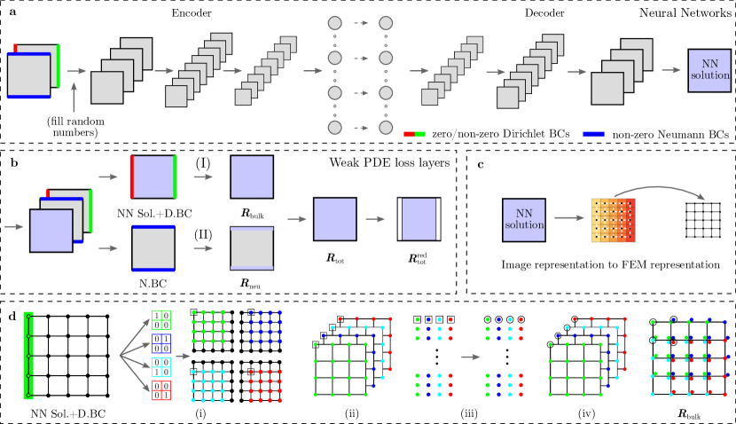
Figure 1: Architecture of the NN-PDE-S. (a) An encoder-decoder NN to store the nonlinear mapping between NN inputs, which consist of the geometry of problem domains and the applied BCs, and the solution of PDEs. Random numbers are given to the pixels in the interior domain of the channel with Dirichlet BCs when working with the augmented dataset with only a few unique boundary value problems. BCs are color coded with red for zero Dirichlet BCs; green for non-zero Dirichlet BCs; blue for non-zero Neumann BCs. (b) Both NN inputs and outputs are passed to the Weak PDE loss layers to calculate the discretized residual, where the bulk residual (I) is computed from NN solutions with imposed Dirichlet BCs and the residual contribution from the Neumann BCs (II) are computed based on NN inputs. The reduced discretized residual by excluding contributions from Dirichlet boundary locations is used to form the loss of both deterministic and probabilistic NNs. (c) Illustration of the construction of finite element meshes from pixelated image representations. (d) Details of the bulk residual calculation (I). Four filters are applied to the NN solutions with imposed Dirichlet BCs to select different nodes (i), resulting in a multi-channel data representation (ii), which has the structure of the local nodes of one finite element. The multi-channel data is reshaped into a two-dimensional matrix to perform residual calculation (iii). The two-dimensional residual matrix is reshaped to a multi-channel data structure (iv) and x reduced sum operations are performed to get the bulk residual, avoiding the time-consuming assembly process in the traditional FEM.

In the proposed PDE solver (Fig. 1), NNs are used to represent the nonlinear mapping between BCs and the resulting solutions of PDEs. The discretized residuals of PDEs are used to construct the losses and therefore regularize the NN’s solutions of PDEs. We studied both deterministic NNs and BNNs, where the uncertainty of the latter is represented by computing the statistical moments of their outputs via the predictive expectation and the predictive variance.

Deterministic NNs have fixed model parameter values, and their losses are mean squared Euclidean norms of the discretized reduced residual vectors. For BNNs, the model parameters are drawn from a posterior distribution that is computed from Bayes’ theorem. The loss of BNNs is formulated using variational inference [39], which consists of a data-independent contribution and a data-dependent contribution. The latter is the log likelihood function, which has the form of a joint distribution of the discretized residual with an added Gaussian noise. Both NNs are trained via a mini-batch optimization process with standard stochastic optimizers.

In the proposed framework, the PDE loss layers (Fig. 1b) are independent of the NNs, which offers flexibility in choosing the NN architecture. An encoder-decoder NN architecture is explored (Fig. 1a). The NNs, which store the nonlinear mappings between BCs and the PDE solutions, accept image-type inputs that contain physically meaningful boundary values and markers for different regions to allow the convolutional NN layers to learn the BCs and problem domain. This allows a well-trained NN to make predictions for new problem domains with new BCs when these are provided as inputs. As the image-type NN outputs can be treated as FEM meshes (Fig. 1c), we evaluate the discretized residuals of PDEs based on the imposed BCs and NN predictions by following the FEM and using standard numerical integration schemes. This is achieved through an efficient, discrete, convolution operator-based, and vectorized implementation. Calculation of the bulk residual is illustrated in Fig. 1d with detailed implementations and procedures provided in the SI.

In this work, we define one unique BVP as imposing a certain PDE on a specific domain with specific boundary values at specific boundary conditions. Changes in any of these elements defines a new boundary value problem. We found that training a single NN to solve multiple boudnary value prooblems with both Dirichlet and Neumann BCs can be very challenging. We introduced a zero-initialization step to address the slower convergence for problems under Neumann BCs (see SI for detailed discussions). When training BNNs to solve multiple boundary value problems simultaneously, their parameters can stagnate around some local minima, leading to poor performance. To address this issue, we use a warm start approach by initializing the mean of a BNN with the optimized parameters from a deterministic NN with the identical architecture. Our method works for both small and large datasets of boundary value problems. If the number of unique boundary value problems is small, we replicate them to obtain an augmented dataset for training.

Steady-state diffusion problem with small dataset

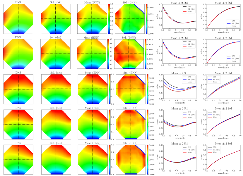
Figure 2: (B)NN-PDE-S for steady-state diffusion. Each row contains the FEM solution (labeled as DNS), solutions from NN-PDE-S, the mean and std of BNN-PDE-S solutions (warm started from the NN-PDE-S), and a quantitative comparison between the FEM solution, the NN-PDE-S solution, and the mean $\pm$ 2 std of BNN-PDE-S results along the two dashed lines. Rows 1 and 2: results for the same boundary value problem with mixed BCs at different mesh resolutions with 32 $\times$ 32 for Row 1 and 64 $\times$ 64 for Row 2. The problem setup for Rows 1 and 2 is shown in the SI. Rows 3-5 results for boundary value problems with identical BCs but different material parameters simultaneously solved by a single (B)NN-PDE-S at a mesh resolution of 32 $\times$ 32.

In this first example (Fig. 2a-b), we use the (B)NN-PDE-S on a single steady-state diffusion boundary value problem on an octagonal domain with imposed mixed BCs (zero/non-zero Dirichlet and non-zero Neumann BCs) at two different mesh resolutions. The DNS solution from FEM, NN solution from a deterministic NN, and the mean and std. of BNN results from 50 Monte Carlo samplings for a mesh resolution of 32 $\times$ 32 are shown in Fig. 2a. The optimized parameters from the deterministic NN are used for the warm start of the BNNs. The deterministic NN results, the mean $\pm$ 2 std of BNN results, and the FEM solution, which is considered the grand truth, are quantitatively commpared along the two dashed lines in Fig. 2a. These quantitative comparisons confirm the accuracy of the NN results. The results in Fig. 2b for a mesh resolution of 64 $\times$ 64 show the same accuracy of the NN results. In the second example (Fig. 2c-e), we use the NN-PDE-S to simultaneously solve three boundary value problems with identical BCs but different material parameters at a mesh resolution of 32 $\times$ 32. The quantitative comparisons in Fig. 2c-e demonstrate the ability of a single, trained NN to simultaneously solve multiple booundary value prooblems.

Linear elasticity problem with small dataset

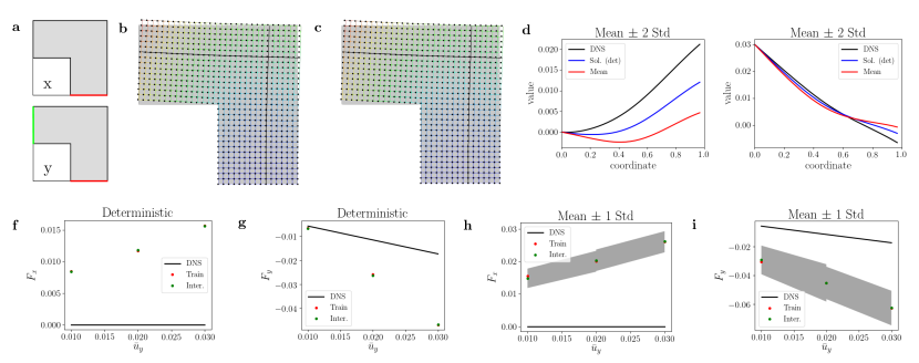
Figure 3: (B)NN-PDE-S for linear elasticity. (a) setup of BCs for the L-shape problem. (b) comparison of solutions between the FEM and the NN-PDE-S. Both solutions are plotted in the deformed configuration with the FEM solution being illustrated by the mesh grid and the deterministic NN solution being illustrated by the solid black dot. (c) similar solution comparison as in (b), but between the FEM solution and the mean of the BNN-PDE-S solutions among 50 Monte Carlo samplings. (d) comparison of displacements in the X-direction along the vertical line and in the Y-direction along the horizontal line among the FEM solution, the NN-PDE-S solution, whose parameters are used to warm start the BNN-PDE-S, and the mean and std of solutions from a BNN-PDE-S for a solution resolution of $32\times 32$. (f, g) comparison of reaction forces in both X- and Y-direction between the FEM and the NN-PDE-S. (h, i) comparison of reaction forces in both $X$ and $Y$-direction between the FEM and the BNN-PDE-S.

It is challenging to solve linear elasticity mainly because the governing PDE is written in terms of the infinitesimal strain, which is the gradient of the displacement field and has a very small magnitude $\sim 10^{-4}$. Here, we use the (B)NN-PDE-S for the displacement on an L-shape domain, which is fixed in both directions on the bottom edge and has a vertical displacement applied on the left edge. A mesh resolution of 32 $\times$ 32 is considered. The problem is defined in Fig. 3a. We consider three incremental loading levels and treat each loading level as a different boundary value problem. The BNN used to solve these boundary value problems is trained with a warm start. The deformed geometries from both the FEM results and the deterministic NN results are compared in Fig. 3b, where the FEM solution is illustrated by the mesh and the NN solution by the solid black dots. The corresponding comparison between the FEM and the mean of the BNN solution is shown in 3c. The quantitative comparisons for $\mbox{\boldmath$u$}_{x}$ along the vertical lines and $\mbox{\boldmath$u$}_{y}$ along the horizontal lines in Fig. 3(b,c) between the FEM results, the deterministic NN solution, and the mean $\pm$ 2 std of BNN results are shown in Fig. 3(d). Those results confirm the accuracy of the NN-based solver. Additionally, we also show the comparison of reaction forces for different loading levels in both the $x-$ and $y-$ directions between the FEM solution and the deterministic NNs (Fig. 3f,g) and between the FEM solution and the mean $\pm$ 2 std of BNN results (Fig. 3h,i). However, because the magnitude of the solution at the bottom of the L-shape is low, the NNs have difficulty computing the total reaction forces. Another example using a single deterministic NN and BNN to solve 30 linear elastic boundary value prooblems for five different domains with six sets of BCs applied to each appears in the SI.

Nonlinear elasticity problem with small dataset

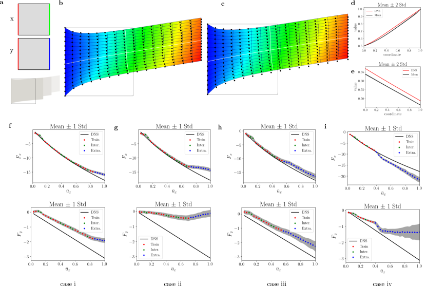
Figure 4: (B)NN-PDE-S for nonlinear elasticity. (a) definition of the boundary value problem for the interpolated and extrapolated loading example. Three loading levels and the deformed shapes are illustrated. (b) Comparison between the FEM solution and the NN-PDE-S solution with a resolution of $16\times 16$ for the last extrapolated BCs for case i. The deformed shapes are plotted with the FEM solution illustrated by the mesh and the NN solution by the solid black dot. (c) The corresponding comparison between the FEM solution and the mean of the BNN-PDE-S solution over 50 MC samplings. (d) Comparison of displacement in the $X$-direction along the horizontal white lines in (b, c) between the solutions of the FEM, the NN-PDE-S whose parameters are used to warm start the BNN-PDE-S, and the mean and std of solutions from the BNN-PDE-S. (e) Similar comparison as in (d), but for displacement in the $Y$-direction along the vertical white lines in (b, c). (f-i) reaction forces in both $X$- and $Y$-directions for four different cases with each containing a different number of training and testing data.

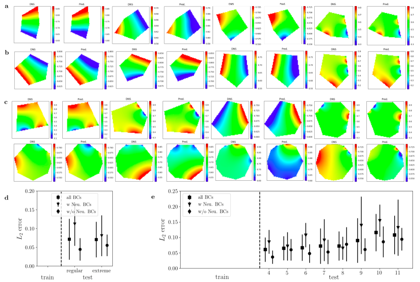
Figure 5: NN-PDE-S for steady-state diffusion with large dataset. (a) Selected good NN-PDE-S predictions for new, randomly generated extreme pentagons. (b) Selected good NN-PDE-S predictions for new, randomly generated regular pentagons. (c) Selected good NN-PDE-S predictions for new, randomly generated polygons with different total numbers of edges. (d) $L_{2}$ error of NN-PDE-S results for the pentagon example study. $L_{2}$ error from all boundary value problems, those with Neumann BCs, and others without Neumann BCs are plotted for both training and testing datasets. (e) $L_{2}$ error of NN-PDE-S results for the polygon example study. $L_{2}$ error from all boundary value problems, those with Neumann BCs, and others without Neumann BCs are plotted for both training and testing datasets.

We use the (B)NN-PDE-S solver framework on a nonlinear elasticity problem on a square domain fixed in both directions on the left edge, and with a horizontal displacement loading and vertical traction loading applied on the right edge. We considered 30 incremental loading levels and treated each as a different boundary value problem, as shown in Fig. 4c. The BNNs are trained with a warm start for four cases. The training dataset for each case has different distributions of loading levels. The testing dataset contains both interpolated and extrapolated loading levels, as indicated by different colors in Fig. 4f-i. The results, including the FEM solution, the deterministic NN, and the mean and std from the BNN, for the last extrapolated loading level for case (i) in both $X$- and $Y$-directions are shown in Fig. 4b and 4c. Additionally, we show the quantitative comparison between FEM results and the mean $\pm$ 2 std of BNN results along the dashed lines (Fig. 4d and 4e). These results confirm the accuracy of the NN-based solver and demonstrate its predictivity for unseen extrapolated BCs. The reaction forces computed from the NN full field solution are plotted in Fig. 4f-i, which shows improved accuracy compared to the results for linear elasticity (Fig. 3f-i). For each case, we observe that the results from interpolated BCs are generally accurate. For extrapolated BCs, NN predictions are accurate to a certain degree, particularly for the reaction force in the $X$-direction. Details of the treatment for computing the nonlinear kinematics, constitutive relations, and discretized residuals with NNs, NN architecture and training scheme, and an additional example on solving 30 boundary value problems with the proposed method are provided in the SI.

Steady-state diffusion problem with large dataset

Lastly, we use the BNN-PDE-S on the steady-state diffusion problem for two very large datasets with a $64\times 64$ resolution. In these datasets, the geometries of problem domains and the values of BCs are randomly generated. The locations of BCs are randomly selected from two non-adjacent edges. The boundary values along one edge could be constant, a linear distribution, quadratic distribution, or sinusoidal distribution. The details of the data generation scheme and the statistics of our datasets are discussed in the SI.

In the first case, the training dataset contains 168,000 unique boundary value problems with pentagons, where none of the inner angles exceed $160^{\circ}$. The testing dataset is newly generated with 80 boundary value problems on pentagons with all angles $<160^{\circ}$ and 80 on “extreme" pentagons (those with at least one angle $\geq 160^{\circ}$). Some of the selected results for different geometries are shown in Fig. 5a, which shows that the trained NNs could predict the solution for unseen geometries, including near-degenerate polygons, and unseen BCs. The accuracy of the NN results is evaluated by the volume averaged $L_{2}$ error across all boundary value problems in the corresponding (training/testing) dataset, which is calculated as

$$\|e\|_{2}=\frac{1}{N_{\mathrm{BVP}}}\sum_{l=1}^{N_{\mathrm{BVP}}}\left(\sqrt{\frac{1}{K_{\mathrm{px}}}\sum_{k=1}^{K_{\mathrm{px}}}\left(y_{l,k}^{\mathrm{DNS}}-y_{l,k}^{\mathrm{NN}}\right)^{2}}\right).$$ (1)

The $L_{2}$ errors of NN results for both training and testing datasets are plotted in Fig. 5(d). We observe that boundary value problems with only Dirichlet BCs generally perform better than those with Neumann BCs.

In the second case, the training dataset contains 192,000 unique boundary value problems with randomly generated geometries of quadrilaterals, pentagons, and hexagons, whereas the testing dataset is newly generated with the number of edges of spanning from four to eleven with 16 boundary value problems for each type of polygon. Some of the selected results for different polygons appear in Fig. 5c, again demonstrating that the trained NNs predict solutions on unseen geometries and unseen BCs. The $L_{2}$ errors of NN results for both training and testing datasets are plotted in Fig. 5(e). We observe some degradation of NN results as the number of polygon edges in the testing set significantly exceed those in the training dataset. However, for training up to hexagons, this degradation in accuracy sets in only for nonagons, decagons and hendecagons.

Table 1: Summary of the accuracy and speed of the (B)NN-PDE-S for the example presented in Fig. 4. Note: There may be speedup of the FEM simulation with further code optimization. The wall times of (B)NN-PDE-S results do not include the time to load the solver.

Solver	Hardware	Software	Wall-time	Averaged $L_{2}$ error
FEM	Intel i7-8750, 2.2GHz (use single core)	mechanoChemFEM	110ms	-
deterministic NN	GeForce GTX 1050 Ti, 4GB memory	Tensorflow	0.22ms	2.45e-3
BNN	GeForce GTX 1050 Ti, 4GB memory	Tensorflow	0.29ms	3.07e-3

Discussion

Our framework successfully learns PDE-specific solvers, whether restricted to a single or multiple boundary problems. It has been our focus to develop solvers that generalize across boundary value problems with different domains, boundary conditions and coefficients, and are orders of magnitude faster than the traditional FEM, as shown in Table 1. Such features distinguish our approach from certain other NN-based PDE solvers [8, 26].

We have used the framework to solve the diffusion problem over two fairly complex, and large datasets of boundary value problems to demonstrate its performance. From the corresponding examples, we observe that the (B)NN-PDE-S makes more accurate predictions for interpolated BCs. To improve its performance, one can manually introduce new BCs to the training dataset to improve the poorly trained region or targeted prediction region; for instance, expanding the dataset with many geometries if prediction across domains is the goal. If the same geometries are considered for training and testing, the dataset could be augmented by filling the interior domain with random numbers. Naturally, good sampling of BCs and boundary locations is important for learning. The performance could further be improved via careful hyper-parameter tuning. The learning or cross-validation error computed over this dataset of $\sim 10^{5}$ boundary value problems with randomly generated polygonal domains (order and shape), boundary conditions and coefficients can be used to drive an active learning workflow that detects regimes (domains, boundary conditions, boundary value functions and coefficients) in which additional boundary value problems are needed for improved learning.

For BNNs, we applied a constant additive noise to the NN solutions, which is propagated through the PDE residual calculation to compute the training loss function. While the additive noise often is used to account for aleatoric uncertainty in Bayesian inference, here it accounts for model form error of the BNN, and thus corresponds to epistemic uncertainty. The applied noise $\Sigma_{1}$ functions as the convergence threshold used in the traditional numerical methods for PDEs. The loss of BNNs consists of data-independent (K-L divergence) and data-dependent (negative log-likelihood) contributions (Methods, Eqs (17-23)). During training, the data-dependent log-likelihood contribution to the loss is, in general much larger than the data-independent K-L divergence, and decreases. As it does, the data-independent K-L divergence weighs more, leading the mean of the BNN solutions to drift away from the ground truth. With training, both contributions decrease and the mean of the BNN solutions gradually converges to the DNS solution. The K-L divergence term tends to introduce more uncertainty to the model parameters especially with poorly informed priors. The log-likelihood, which depends on $\Sigma_{2}$ tends to reduce the uncertainty. It controls convergence of the NN solution to the DNS solution as $\Sigma_{2}$ itself converges. We report the evolution of $\Sigma_{2}$ in Figs S21, S25 and SS29.

We use a “warm start” by initializing the means of the BNN parameters to the optimized parameters from deterministic NNs with an identical architecture. An alternative is to initialize the means of the prior to the optimized parameters from deterministic NNs.

BVPs with very small variations in the solutions, such as the L-shape linear elasticity example, pose challenges since the NNs have difficulty capturing small differences. Formally, of course, these problems have low information content. Additionally, the linear elasticity residual is determined by the displacement gradient (infinitesimal strain) field, which is invariant to data normalization. We found that though the residual is computed from the physical, un-normalized, solution, learning is more effective with data normalization. It ensures that the variations of NN outputs (scaled solution) is large $\in[-1,1]$ unlike the infinitesimal strain $\sim 10^{-4}$. Large variations in the NN outputs drive NN parameter variations and favor training. This also applies to diffusion when the solution range is very small. In the residual-based loss, however, the NN output is scaled back to the physical range, to prevent violation of physics.

Hyper-parameter searches are essential for optimal (B)NN-PDE-S. The PDEs differ in their optimal hyperparameters. NNs targeted at solving a wider range of steady state diffusion boundary value problems required wider layers. The vector elasticity problems, even with isotropic properties, have greater information content in their solution field and in general demanded wider layers. The numbers of layers were more closely aligned, and optimal kernel sizes were the same across the PDEs and targeted boundary value problem ranges. See Tables S1, S3, S6, S8, S10, S12.

The NN solvers presented here were trained on a single GeForce GTX 1050 Ti GPU with 4GB memory. Training could take hours for networks designed to solve $\sim 20$ boundary value problems, and days for those to solve $\sim 10^{5}$ of boundary value problems. In addition to more high-powered GPUs, as well as multi-GPU training, optimization of the training workflow remains unexplored. The training time would be further reduced if transfer learning or multi-fidelity learning is used by continued training of previously trained networks. Training the (B)NN-PDE-S takes more time than training regular NNs because of the PDE constrained loss layer. The prediction time, however, is unaffected by these loss layers, as they are not activated during prediction.

In this work, the problem domains are represented via pixels on a square background grid for simplicity. Thus, domain boundaries are not smooth curves, but have a pixel-level resolution. This treatment is of importance as it applies directly to solving PDEs on pixel-based, experimental images as domain data–a target future application for our work. For smooth boundary representations, one can leverage recent work for approaches to map complex and irregular domains onto a regular mesh [3, 4, 26]. Such geometric transformations can be taken into account in the proposed PDE loss layers, for instance via the mapping of the physical domain from parent hyper-cubes, as is commonly done in the FEM. While we have considered polygonal domains for their approximation of other geometries, the above mapping could be exploited to remove this restriction, also.

Our approach is formally different from recent operator networks which are focused on learning nonlinear mappings between input function spaces and output spaces, and therefore are mesh independent. In this regard we note that a NN solver that has learnt a PDE on a given discretization (pixel resolution) can serve as the source network for a target finer or coarser mesh within a transfer learning context. The most important difference between the presented (B)NN-PDE-S and DeepONets [35, 36], graph kernel networks [37] and Fourier operator networks [38] is that these operator network approaches need labelled field data for training–typically from DNS using the underlying PDE. By not presenting and labelled field solution, but only the domain, BCs and coefficients to the network, our approach in addition to being label free allows room for our claim that the network is forced to learn the PDE, which by definition holds across boundary value problems. We note that the recent TL-DeepONet [36] uses a source Banach space from a DeepONet trained on labelled data for specific boundary conditions. Further training the final layer of the TL-DeepONet allows transfer learning to some new boundary value problems. We are not aware of the extensiveness to which this transfer learning across boundary value problems has been studied by the authors. Our approach is very appealing for high-throughput solution of PDEs ranging from inverse and other optimization problems through design and decision-making. Its generalizability across domains and boundary conditions also presents opportunities in topology optimization problems. Ongoing developments will extend it beyond elliptic PDEs.

Methods

General elliptic PDEs In this work, we develop (B)NN-PDE-S for steady-state diffusion, linear elasticity, and nonlinear elasticity. These three physical systems are described by a general elliptic PDE on a continuum domain $\Omega\subset\mathbb{R}^{n}$ with Dirichlet BCs on $\Gamma^{\mbox{\boldmath$\varphi$}}$ and the Neumann BCs on $\Gamma^{{\bm{\mathnormal{k}}}}$:

$$\nabla\cdot{\bm{\mathnormal{A}}}(\mbox{\boldmath$\varphi$})={\bm{\mathit{0}}} \text{on}\quad\Omega,$$ (2)

$$\mbox{\boldmath$\varphi$}({\bm{\mathnormal{X}}})=\bar{\mbox{\boldmath$\varphi$}}({\bm{\mathnormal{X}}}) \text{on}\quad\Gamma^{\mbox{\boldmath$\varphi$}},$$

$${\bm{\mathnormal{k}}}({\bm{\mathnormal{X}}})=\bar{{\bm{\mathnormal{k}}}}({\bm{\mathnormal{X}}}) \text{on}\quad\Gamma^{\bm{\mathnormal{k}}},$$

where $\mbox{\boldmath$\varphi$}({\bm{\mathnormal{X}}})$ represents the spatially-dependent unknown field and ${\bm{\mathnormal{X}}}\in\mathbb{R}^{n}$ is the position vector. The boundary of the continuum domain satisfies $\overline{\Gamma}=\overline{\Gamma^{\mbox{\boldmath$\varphi$}}\bigcup\Gamma^{{\bm{\mathnormal{k}}}}}$ and $\Gamma^{\mbox{\boldmath$\varphi$}}\bigcap\Gamma^{{\bm{\mathnormal{k}}}}=\emptyset$. We use bold typeface for $\varphi$, ${\bm{\mathnormal{A}}}$, and ${\bm{\mathnormal{k}}}$ in (2), depending on the physical system, they could represent either scalar, vector, or tensor fields. For example, in the diffusion problem, $\varphi$, ${\bm{\mathnormal{A}}}$, and ${\bm{\mathnormal{k}}}$ represent the compositional order parameter (scalar), the diffusive flux (vector), and the outflux (scalar), respectively, whereas in elasticity problems, $\varphi$, ${\bm{\mathnormal{A}}}$, and ${\bm{\mathnormal{k}}}$ represent the deformation field (vector), the stress field (second-order tensor), and the surface traction (vector), respectively. The details of each system appear below.

The weak form of (2) states: For variations $\omega$ satisfying $\forall\mbox{\boldmath$\omega$}\in\mathscr{V}$ with $\mathscr{V}=\left\{\mbox{\boldmath$\omega$}|\mbox{\boldmath$\omega$}={\bm{\mathit{0}}}~{}\text{on}~{}\Gamma^{\mbox{\boldmath$\varphi$}}\right\}$, seek trial solutions $\mbox{\boldmath$\varphi$}\in\mathscr{S}$ with $\mathscr{S}=\left\{\mbox{\boldmath$\varphi$}|\mbox{\boldmath$\varphi$}=\bar{\mbox{\boldmath$\varphi$}}~{}\text{on}~{}\Gamma^{\mbox{\boldmath$\varphi$}}\right\}$ such that

$$\int_{\Omega}\nabla\mbox{\boldmath$\omega$}\cdot{\bm{\mathnormal{A}}}(\mbox{\boldmath$\varphi$})~{}dV-\int_{\Gamma^{\bm{\mathnormal{k}}}}\bar{{\bm{\mathnormal{k}}}}\cdot\mbox{\boldmath$\omega$}~{}dS=0.$$ (3)

Eq. (3) is obtained by multiplying (2₁) with $\omega$, integrating by parts, and then incorporating the Neumann BC in (2₃). For the diffusion problem, $\omega$ is a scalar field. For elasticity problems, $\omega$ is a vector field.

Approximate, numerical solutions of (3) can be obtained using its finite-dimensional form. Finite-dimensional approximations of $\omega$ and $\varphi$, denoted by $\mbox{\boldmath$\omega$}^{h}$ and $\mbox{\boldmath$\varphi$}^{h}$, are constructed with $\mbox{\boldmath$\omega$}^{h}\in\mathscr{V}^{h}=\left\{\mbox{\boldmath$\omega$}^{h}|\mbox{\boldmath$\omega$}^{h}={\bm{\mathit{0}}}~{}\text{on}~{}\Gamma^{\mbox{\boldmath$\varphi$}}\right\}$ and $\mbox{\boldmath$\varphi$}^{h}\in\mathscr{S}^{h}=\left\{\mbox{\boldmath$\varphi$}^{h}|\mbox{\boldmath$\varphi$}^{h}=\bar{\mbox{\boldmath$\varphi$}}~{}\text{on}~{}\Gamma^{\mbox{\boldmath$\varphi$}}\right\}$. The finite-dimensional fields $\mbox{\boldmath$\omega$}^{h}$, $\nabla\mbox{\boldmath$\omega$}^{h}$, and $\mbox{\boldmath$\varphi$}^{h}$ are computed as

$$\mbox{\boldmath$\omega$}^{h}={\bm{\mathnormal{N}}}{\bm{\mathnormal{d}}}_{\mbox{\boldmath$\omega$}},\quad\nabla\mbox{\boldmath$\omega$}^{h}={\bm{\mathnormal{B}}}{\bm{\mathnormal{d}}}_{\mbox{\boldmath$\omega$}},\quad\text{and}\quad\mbox{\boldmath$\varphi$}^{h}={\bm{\mathnormal{N}}}{\bm{\mathnormal{d}}}_{\mbox{\boldmath$\varphi$}}$$ (4)

in terms of the nodal solutions ${\bm{\mathnormal{d}}}_{\mbox{\boldmath$\omega$}}$ and ${\bm{\mathnormal{d}}}_{\mbox{\boldmath$\varphi$}}$, the basis functions ${\bm{\mathnormal{N}}}$, and the basis function gradient operator ${\bm{\mathnormal{B}}}=\nabla{\bm{\mathnormal{N}}}$. Inserting (4) into (3) we obtain the discretized residual as an assembly over subdomains $\Omega^{e}$ and their associated boundary $\Gamma^{e}$ as

$${\bm{\mathnormal{R}}}=\operatorname*{\scalerel*{A}{\sum}}_{e=1}^{n_{\text{elem}}}\left\{\int_{\Omega^{e}}{\bm{\mathnormal{B}}}^{T}{\bm{\mathnormal{A}}}(\mbox{\boldmath$\varphi$}^{h})dV-\int_{\Gamma^{e,{\bm{\mathnormal{k}}}}}{\bm{\mathnormal{N}}}^{T}\bar{{\bm{\mathnormal{k}}}}~{}dS\right\}$$ (5)

where $\operatorname*{\scalerel*{A}{\sum}}$ is the assembly operator and $n_{\text{elem}}$ represents the total number of subdomains. The volume and surface integrations in (5) are evaluated numerically via Gaussian quadrature rules. In this work, the problem domain $\Omega$ is treated as an image. Single component, connected graphs whose vertices are pixels form the subdomains $\Omega^{e}$. Pixel connectivity is preserved as graph edges in the image data. Field values at each pixel of the image are treated as nodal values. Additional discussion on constructing the subdomains based on image pixels is provided in the SI. Of interest, but tangential, in this context is a recent work in which NN layers map between FE meshes of different resolutions [40].

Steady-state diffusion This problem is described by a linear elliptic PDE in the scalar composition field following (2)

$$\nabla\cdot{\bm{\mathnormal{H}}}={\bm{\mathit{0}}} \text{on}\quad\Omega,$$ (6)

$$C({\bm{\mathnormal{X}}})=\bar{C}({\bm{\mathnormal{X}}}) \text{on}\quad\Gamma^{C},$$

$$H=\bar{H}({\bm{\mathnormal{X}}}) \text{on}\quad\Gamma^{H}.$$

In (6), $C$ represents the composition, ${\bm{\mathnormal{H}}}$ is the diffusive flux defined as

$${\bm{\mathnormal{H}}}=-D\nabla C,$$ (7)

with $D$ as the diffusivity, and $H$ is the outward surface flux in the normal direction. The discretized residual function (5) for steady-state diffusion is written as

$${\bm{\mathnormal{R}}} =\operatorname*{\scalerel*{A}{\sum}}_{e=1}^{n_{\text{elem}}}\left\{\int_{\Omega^{e}}{\bm{\mathnormal{B}}}^{T}{\bm{\mathnormal{H}}}dV-\int_{\Gamma^{e,H}}{\bm{\mathnormal{N}}}^{T}\bar{H}~{}dS\right\}.$$ (8)

Diffusivity $D\in[1.0,100.0]$ has been used.

Linear elasticity This problem also is posed as a linear elliptic PDE, but in terms of a vector field, ${\bm{\mathnormal{u}}}\in\mathbb{R}^{n}$. Following (2) we have:

$$\nabla\cdot\mbox{\boldmath$\sigma$}={\bm{\mathit{0}}} \text{on}\quad\Omega,$$ (9)

$${\bm{\mathnormal{u}}}({\bm{\mathnormal{X}}})=\bar{{\bm{\mathnormal{u}}}}({\bm{\mathnormal{X}}}) \text{on}\quad\Gamma^{{\bm{\mathnormal{u}}}},$$

$${\bm{\mathnormal{T}}}=\bar{{\bm{\mathnormal{T}}}}({\bm{\mathnormal{X}}}) \text{on}\quad\Gamma^{\bm{\mathnormal{T}}}.$$

In (9), ${\bm{\mathnormal{u}}}$ represents the displacement field, $\sigma$ is the stress tensor, and ${\bm{\mathnormal{T}}}$ is the surface traction. Here, $\sigma$ is related to the infinitesimal strain $\mbox{\boldmath$\varepsilon$}=\frac{1}{2}\left(\nabla{\bm{\mathnormal{u}}}+(\nabla{\bm{\mathnormal{u}}})^{T}\right)$ via the following constitutive relationship

$$\mbox{\boldmath$\sigma$}=\lambda\text{tr}(\mbox{\boldmath$\varepsilon$}){\bm{\mathit{1}}}+2\mu\mbox{\boldmath$\varepsilon$}$$ (10)

where $\lambda$ and $\mu$ are the Lamé constants, and ${\bm{\mathit{1}}}$ is the second-order identity tensor. The discretized residual function (5) for the linear elasticity problem is written as

$${\bm{\mathnormal{R}}}=\operatorname*{\scalerel*{A}{\sum}}_{e=1}^{n_{\text{elem}}}\left\{\int_{\Omega^{e}}{\bm{\mathnormal{B}}}^{T}\mbox{\boldmath$\sigma$}dV-\int_{\Gamma^{e,T}}{\bm{\mathnormal{N}}}^{T}\bar{{\bm{\mathnormal{T}}}}~{}dS\right\}.$$ (11)

We used $\lambda=14.4231$ and $\mu=9.61538$ in both DNSs with FEM for comparison with the (B)NN-PDE-S and in the PDE loss layers.

Nonlinear elasticity With the displacement ${\bm{\mathnormal{u}}}\in\mathbb{R}^{n}$ as the vector field unknown, we write following (2):

$$\nabla\cdot{\bm{\mathnormal{P}}}={\bm{\mathit{0}}} \text{on}\quad\Omega_{0},$$ (12)

$${\bm{\mathnormal{u}}}({\bm{\mathnormal{X}}})=\bar{{\bm{\mathnormal{u}}}}({\bm{\mathnormal{X}}}) \text{on}\quad\Gamma^{{\bm{\mathnormal{u}}}}_{0},$$

$${\bm{\mathnormal{T}}}=\bar{{\bm{\mathnormal{T}}}}({\bm{\mathnormal{X}}}) \text{on}\quad\Gamma^{\bm{\mathnormal{T}}}_{0},$$

for the nonlinear elasticity problem, with the subscript $0$ indicating the reference configuration. In (12), ${\bm{\mathnormal{P}}}$ is the first Piola-Kirchhoff stress tensor, and ${\bm{\mathnormal{T}}}$ is the surface traction. In the nonlinear elasticity problem, the deformation gradient is defined as ${\bm{\mathnormal{F}}}={\bm{\mathit{1}}}+\partial{\bm{\mathnormal{u}}}/\partial{\bm{\mathnormal{X}}}$ with ${\bm{\mathit{1}}}$ being the second-order identity tensor. The right Cauchy-Green deformation tensor is written as ${\bm{\mathnormal{C}}}={\bm{\mathnormal{F}}}^{T}{\bm{\mathnormal{F}}}$. The following compressible Neo-hookean hyperelastic free energy function is considered

$$W=\frac{1}{2}\mu(\text{tr}({\bm{\mathnormal{C}}})3-3-2\ln(J))+\lambda\frac{1}{2}(J-1)^{2},$$ (13)

with $\mu$ and $\lambda$ as the Lamé constants and $J=\det(F)$. The Piola stress tensor ${\bm{\mathnormal{P}}}$ is computed as

$${\bm{\mathnormal{P}}}=\frac{\partial W}{\partial{\bm{\mathnormal{F}}}}=\lambda(J^{2}-J){\bm{\mathnormal{F}}}^{-T}+\mu({\bm{\mathnormal{F}}}-{\bm{\mathnormal{F}}}^{-T}).$$ (14)

The discretized residual function (5) for the nonlinear elasticity problem is written as

$${\bm{\mathnormal{R}}}=\operatorname*{\scalerel*{A}{\sum}}_{e=1}^{n_{\text{elem}}}\left\{\int_{\Omega^{e}}{\bm{\mathnormal{B}}}^{T}{\bm{\mathnormal{P}}}dV-\int_{\Gamma^{e,T}}{\bm{\mathnormal{N}}}^{T}\bar{{\bm{\mathnormal{T}}}}~{}dS\right\}.$$ (15)

The same Lamé constants were used as in linear elasticity.

Deterministic loss When using mini-batch optimization to train the NN-PDE-S over a dataset ${\mathcal{D}}$, where each data point is a boundary value problem with information on problem domain and BCs, the batch loss ${\mathcal{L}}_{i}$ is written in terms of the reduced total residual ${\bm{\mathnormal{R}}}_{\text{tot}}^{\text{red}}$, as illustrated in Fig. 1, as

$${\mathcal{L}}_{i}=\frac{1}{N}\sum_{n=1}^{N}\left({\bm{\mathnormal{R}}}_{\text{tot}}^{\text{red}}({\mathcal{D}}_{i},\mbox{\boldmath$\Theta$})\right)^{2},$$ (16)

for each mini-batch $i=1,2,\cdots,M$ with $N$ indicating the number of data points (boundary value problems) in each mini-batch. The detailed training of NN-PDE-S is discussed in the SI.

Probabilistic loss In BNN-PDE-S, each model parameter is sampled from a posterior distribution. We solve for the posterior distribution of model parameters with variational inference instead of Markov Chain Monte Carlo (MCMC) sampling, as the latter involves expensive iterative inference steps and is not suitable for systems with a large number of parameters [39, 41]. In our work, the likelihood function is constructed based on the discretized PDE residuals. An additive noise is often applied to the NN predicted solution to represent the aleatoric uncertainty [42, 43, 10, 1, 9]. Here, we also applied an additive noise to the solution to represent epistemic uncertainty stemming from model form error between BNN-PDE-S, whose perturbed solutions are still constrained by the PDEs, and the FEM solver that yields the DNS solution.

The BNN model parameters $\Theta$ are stochastic and sampled from a posterior distribution $P(\mbox{\boldmath$\Theta$}|{\mathcal{D}})$ instead of being represented by single values as in deterministic NNs. The posterior distribution $P(\mbox{\boldmath$\Theta$}|{\mathcal{D}})$ is computed based on Bayes’ theorem

$$P(\mbox{\boldmath$\Theta$}|{\mathcal{D}})=\frac{P({\mathcal{D}}|\mbox{\boldmath$\Theta$})P(\mbox{\boldmath$\Theta$})}{P({\mathcal{D}})},$$ (17)

where ${\mathcal{D}}$ denotes the i.i.d. observations (training data) and $P$ represents the probability density function. In (17), $P({\mathcal{D}}|\mbox{\boldmath$\Theta$})$ is the likelihood, $P(\mbox{\boldmath$\Theta$})$ is the prior probability, and $P({\mathcal{D}})$ is the evidence, respectively. The likelihood is the probability of ${\mathcal{D}}$ given $\Theta$, which describes the probability of the observed data for given parameters $\Theta$. A larger value of $P({\mathcal{D}}|\mbox{\boldmath$\Theta$})$ implies that $\Theta$ is more likely to yield ${\mathcal{D}}$. The prior must be specified to begin Bayesian inference [44].

To compute the posterior distributions of $\Theta$, one can use popular sampling-based methods, such as MCMC. However, MCMC involves expensive iterative inference steps and would be difficult to use when datasets are large or models are very complex [41, 45, 39]. An alternative is variational inference, which approximates the exact posterior distribution $P(\mbox{\boldmath$\Theta$}|{\mathcal{D}})$ with a more tractable surrogate distribution $Q(\mbox{\boldmath$\Theta$})$ by minimizing the Kullback-Leibler (KL) divergence [45, 39, 46]

$$Q^{*}=\text{arg~{}min}~{}D_{\text{KL}}(Q(\mbox{\boldmath$\Theta$})||P(\mbox{\boldmath$\Theta$}|{\mathcal{D}})).$$ (18)

Variational inference is faster than MCMC and easier to scale to large datasets. We therefore explore it in this work, even though it is less rigorously studied than MCMC [39]. The KL divergence is computed as

$$D_{\text{KL}}(Q(\mbox{\boldmath$\Theta$})||P(\mbox{\boldmath$\Theta$}|{\mathcal{D}}))=\mathbb{E}_{Q}[\log Q(\mbox{\boldmath$\Theta$})]-\mathbb{E}_{Q}[\log P(\mbox{\boldmath$\Theta$},{\mathcal{D}})]+\log P({\mathcal{D}}),$$ (19)

which requires computing the logarithm of the evidence, $\text{log}P({\mathcal{D}})$ in (17) [39]. However, computation of $P({\mathcal{D}})$ would require marginalization over all realizations of $\Theta$–an intractable task. It is also difficult to estimate $P({\mathcal{D}})$. Consequently, it is challenging to directly evaluate the objective function in (18). Alternatively, we can optimize the so-called evidence lower bound (ELBO) which is equivalent to the KL-divergence up to an added constant. Therefore, an optimal distribution determined using the ELBO is also optimal for the KL-divergence.

$$\text{ELBO}(Q) =-D_{\text{KL}}(Q(\mbox{\boldmath$\Theta$})||P(\mbox{\boldmath$\Theta$}|{\mathcal{D}}))+\log P({\mathcal{D}})$$ (20)

$$\text{ELBO}(Q) =\mathbb{E}_{Q}[\log P(\mbox{\boldmath$\Theta$},{\mathcal{D}})]-\mathbb{E}_{Q}[\log Q(\mbox{\boldmath$\Theta$})]$$

$$=\mathbb{E}_{Q}[\log P({\mathcal{D}}|\mbox{\boldmath$\Theta$})]-\left(\mathbb{E}_{Q}[\log Q(\mbox{\boldmath$\Theta$})]-\mathbb{E}_{Q}[\log P(\mbox{\boldmath$\Theta$})]\right)$$

$$=\mathbb{E}_{Q}[\log P({\mathcal{D}}|\mbox{\boldmath$\Theta$})]-D_{\text{KL}}\left(Q(\mbox{\boldmath$\Theta$})||P(\mbox{\boldmath$\Theta$})\right).$$

So, the loss function for the BNN is written as

$${\mathcal{L}}=D_{\text{KL}}\left(Q(\mbox{\boldmath$\Theta$})||P(\mbox{\boldmath$\Theta$})\right)-\mathbb{E}_{Q}[\log P({\mathcal{D}}|\mbox{\boldmath$\Theta$})],$$ (21)

which consists of a prior-dependent but data-independent part and a data-dependent part. The former is the KL-divergence of the surrogate posterior distribution $Q(\mbox{\boldmath$\Theta$})$ and the prior $P(\mbox{\boldmath$\Theta$})$, and the latter is the negative log-likelihood. For mini-batch optimization, the batch loss is written as

$${\mathcal{L}}_{i}=\frac{1}{M}D_{\text{KL}}\left(Q(\mbox{\boldmath$\Theta$})||P(\mbox{\boldmath$\Theta$})\right)-\mathbb{E}_{Q}[\log P({\mathcal{D}}_{i}|\mbox{\boldmath$\Theta$}^{(i)})],$$ (22)

for each mini-batch $i=1,2,\cdots,M$ [47]. With (22), we have ${\mathcal{L}}=\sum_{i}{\mathcal{L}}_{i}$. Following Ref [47], Monte Carlo (MC) sampling is used to approximate the expectation in (22) as

$${\mathcal{L}}_{i}\approx\frac{1}{M}D_{\text{KL}}\left(Q(\mbox{\boldmath$\Theta$})||P(\mbox{\boldmath$\Theta$})\right)-\frac{1}{N}\sum_{n=1}^{N}\log P({\mathcal{D}}_{i}^{n}|\mbox{\boldmath$\Theta$}^{(i)}),$$ (23)

where $N$ is the size of each mini-batch dataset, and $\mbox{\boldmath$\Theta$}^{(i)}$ denotes the $i$th batch sample drawn from the posterior distribution $Q(\mbox{\boldmath$\Theta$})$. Even though only one set of parameters $\mbox{\boldmath$\Theta$}^{(i)}$ is drawn from $Q(\mbox{\boldmath$\Theta$})$ for each mini-batch, the perturbation approach proposed by Flipout (see SI) ensures that parameters are de-correlated for each individual example ${\mathcal{D}}_{i}^{n}$ in calculating the log-likelihood. Probabilistic dense layers and convolutional layers with the Flipout weight perturbation technique have been implemented in the TFP Library and are used to construct the BNNs in this work.

Neural network structure and loss function Using modularized implementation of probabilistic layers in the TFP library it is easy to construct the BNN-PDE-S to have the encoder-decoder architecture shown in Fig. 1, which is similar to the NN-PDE-S but with all weights being drawn from probability distributions. The loss of the BNNs is given in (21). The probabilistic layers in the TFP library automatically calculate the prior-dependent KL-divergence and add it to the total loss.

The data-dependent loss is accounted for by the likelihood. Assuming Gaussian noise $\mbox{\boldmath$\epsilon$}\sim{\mathcal{N}}({\bm{\mathit{0}}},\Sigma_{1}{\bm{\mathnormal{I}}})$ with a zero-mean and a pre-specified constant covariance $\Sigma_{1}$, the NN representation ${\bm{\mathnormal{f}}}({\bm{\mathnormal{x}}},\mbox{\boldmath$\Theta$})$ is augmented by noise to yield the output ${\bm{\mathnormal{y}}}$:

$${\bm{\mathnormal{y}}}={\bm{\mathnormal{f}}}({\bm{\mathnormal{x}}},\mbox{\boldmath$\Theta$})+\mbox{\boldmath$\epsilon$}.$$ (24)

Forward solutions are obtained by seeking to drive the residual to zero, and correspond to satisfaction of the weak form. For BNN-PDE-S, the likelihood function is constructed from the residual value, rather than the NN predicted solutions, thus ensuring that the framework remains label free. With the noise $\epsilon$ in (24) propagating through the residual calculation, the likelihood function is written as

$$P({\bm{\mathnormal{R}}}_{\text{tot}}^{\text{red}}({\mathcal{D}}_{i},\mbox{\boldmath$\Theta$}^{(i)})|{\bm{\mathit{0}}},\Sigma{\bm{\mathnormal{I}}})=\prod_{k=1}^{K}{\mathcal{N}}\left(R_{\text{tot}}^{\text{red,$k$}}|0,\Sigma_{2}\right)$$ (25)

where index $k$ indicates the pixel number with $K$ total pixels and ${\bm{\mathnormal{R}}}_{\text{tot}}^{\text{red},k}$ is the component of ${\bm{\mathnormal{R}}}_{\text{tot}}^{\text{red}}$ at pixel $k$. For systems where nonlinear operations are involved in the residual calculation, the residual noise distribution is in general non Gaussian even if the noise in the BNN outputs is assumed to be Gaussian. Under the conditions that $\Sigma_{1}$ is small and the nonlinear operations are smooth, there exists a neighborhood of any point in which the linear approximation is valid (higher-order terms being negligible), we assume that $\Sigma_{2}$, the noise distribution of the residual, is approximately Gaussian. As it is challenging to directly calculate $\Sigma_{2}$ via error propagation based on $\Sigma_{1}$, we treat $\Sigma_{2}$ as a learnable parameter to be optimized based on the NN loss. In (25), $\Sigma_{2}$ essentially serves as a convergence threshold for the residual. The batch-wise loss of the residual constrained BNNs has the following form

$${\mathcal{L}}_{i}\approx\frac{1}{M}D_{\text{KL}}\left(Q(\mbox{\boldmath$\Theta$})||P(\mbox{\boldmath$\Theta$})\right)-\frac{1}{N}\sum_{n=1}^{N}\sum_{k=1}^{K}\log\left({\mathcal{N}}\left(R_{\text{tot}}^{\text{red,$k$}}({\mathcal{D}}_{i}^{n},\mbox{\boldmath$\Theta$}^{(i)})|0,\Sigma_{2}\right)\right).$$ (26)

The detailed training scheme for BNN-PDE-S is discussed in the SI.

Uncertainty quantification The BNNs allow us to quantify the epistemic uncertainty from model parameters. With the discretized residual constrained BNNs, the posterior predictive distribution $P({\bm{\mathnormal{y}}}^{*}|{\bm{\mathnormal{x}}}^{*},{\mathcal{D}})$ of the BNN-predicted full field solution ${\bm{\mathnormal{y}}}^{*}$ for a specific testing data point ${\bm{\mathnormal{x}}}^{*}$, i.e. one boundary value problem with information on problem domain and BCs is [1, 42]

$$P({\bm{\mathnormal{y}}}^{*}|{\bm{\mathnormal{x}}}^{*},{\mathcal{D}}) =\int P({\bm{\mathnormal{y}}}^{*}|{\bm{\mathnormal{x}}}^{*},\mbox{\boldmath$\Theta$})P(\mbox{\boldmath$\Theta$}|{\mathcal{D}})d\mbox{\boldmath$\Theta$}$$ (27)

$$\approx\int P({\bm{\mathnormal{y}}}^{*}|{\bm{\mathnormal{x}}}^{*},\mbox{\boldmath$\Theta$})Q(\mbox{\boldmath$\Theta$})d\mbox{\boldmath$\Theta$},$$

which can be numerically evaluated via MC sampling as

$$P({\bm{\mathnormal{y}}}^{*}|{\bm{\mathnormal{x}}}^{*},{\mathcal{D}}) \approx\frac{1}{S}\sum_{s=1}^{S}P({\bm{\mathnormal{y}}}^{*}|{\bm{\mathnormal{x}}}^{*},\mbox{\boldmath$\Theta$}^{s})\quad\text{where}\quad\mbox{\boldmath$\Theta$}^{s}\sim Q(\mbox{\boldmath$\Theta$}),$$ (28)

with $s$ indicating each sampling. To represent the uncertainty, we compute the statistical moments of ${\bm{\mathnormal{y}}}^{*}$ via the predictive expectation

$$\mathbb{E}[{\bm{\mathnormal{y}}}^{*}|{\bm{\mathnormal{x}}}^{*},{\mathcal{D}}]\approx\frac{1}{S}\sum_{s=1}^{S}{\bm{\mathnormal{f}}}({\bm{\mathnormal{x}}}^{*},\mbox{\boldmath$\Theta$}^{s})$$ (29)

and the predictive variance

$$\text{Var}[{\bm{\mathnormal{y}}}^{*}|{\bm{\mathnormal{x}}}^{*},{\mathcal{D}}] =\mathbb{E}[({\bm{\mathnormal{y}}}^{*}+\mbox{\boldmath$\epsilon$})^{2}]-(\mathbb{E}[{\bm{\mathnormal{y}}}^{*}+\mbox{\boldmath$\epsilon$}])^{2}$$ (30)

$$\approx\frac{1}{S}\sum_{s=1}^{S}\left({\bm{\mathnormal{f}}}({\bm{\mathnormal{x}}}^{*},\mbox{\boldmath$\Theta$}^{s}){\bm{\mathnormal{f}}}^{T}({\bm{\mathnormal{x}}}^{*},\mbox{\boldmath$\Theta$}^{s})+\Sigma_{1}{\bm{\mathnormal{I}}}\right)-\left(\frac{1}{S}\sum_{s=1}^{S}{\bm{\mathnormal{f}}}({\bm{\mathnormal{x}}}^{*},\mbox{\boldmath$\Theta$}^{s})\right)\left(\frac{1}{S}\sum_{s=1}^{S}{\bm{\mathnormal{f}}}({\bm{\mathnormal{x}}}^{*},\mbox{\boldmath$\Theta$}^{s})\right)^{T}.$$

Code Availability

Our modularized code implementation is publicly available, which will assist the extension to other PDE systems.

Author Contributions

Competing Interests statement

References

- [1] Yinhao Zhu and Nicholas Zabaras. Bayesian deep convolutional encoder-decoder networks for surrogate modeling and uncertainty quantification. J. Comput. Phys., 366:415–447, 2018.
- [2] Nick Winovich, Karthik Ramani, and Guang Lin. ConvPDE-UQ: Convolutional neural networks with quantified uncertainty for heterogeneous elliptic partial differential equations on varied domains. J. Comput. Phys., 394:263–279, 2019.
- [3] Saakaar Bhatnagar, Yaser Afshar, Shaowu Pan, and Karthik Duraisamy. Prediciton of Aerodynamic Flow Fields Using Convolutional Neural Networks. Comput. Mech., 5:1–30, 2019.
- [4] Angran Li, Ruijia Chen, Amir Barati Farimani, and Yongjie Jessica Zhang. Reaction diffusion system prediction based on convolutional neural network. Sci. Rep., 10:1–9, 2020.
- [5] Isaac Lagaris, Aristidis Likas, and Dimitrios I. Fotiadis. Artificial neural networks for solving ordinary and partial differential equations. IEEE Transactions on Neural Networks, 9:987–1000, 1998.
- [6] Jiequn Han, Arnulf Jentzen, Weinan E, and E. Weinan. Solving high-dimensional partial differential equations using deep learning. Proceedings of the National Academy of Sciences, 115:8505–8510, 2018.
- [7] Justin Sirignano and Konstantinos Spiliopoulos. DGM: A deep learning algorithm for solving partial differential equations. J. Comput. Phys., 375:1339–1364, 2018.
- [8] Maziar Raissi, Paris Perdikaris, and George E. Karniadakis. Physics-informed neural networks: A deep learning framework for solving forward and inverse problems involving nonlinear partial differential equations. J. Comput. Phys., 378:686–707, 2019.
- [9] Yinhao Zhu, Nicholas Zabaras, Phaedon Stelios Koutsourelakis, and Paris Perdikaris. Physics-constrained deep learning for high-dimensional surrogate modeling and uncertainty quantification without labeled data. J. Comput. Phys., 394:56–81, 2019.
- [10] Nicholas Geneva and Nicholas Zabaras. Modeling the dynamics of PDE systems with physics-constrained deep auto-regressive networks. J. Comput. Phys., 403:109056, 2020.
- [11] Liu Yang, Xuhui Meng, and George Em Karniadakis. B-PINNs: Bayesian physics-informed neural networks for forward and inverse PDE problems with noisy data. J. Comput. Phys., 425:109913, 2021.
- [12] Jens Berg and Kaj Nystroem. A unified deep artificial neural network approach to partial differential equations in complex geometries. Neurocomputing, 317:28–41, 2018.
- [13] Luning Sun, Han Gao, Shaowu Pan, and Jian Xun Wang. Surrogate modeling for fluid flows based on physics-constrained deep learning without simulation data. Comput. Methods Appl. Mech. Engrg., 361:112732, 2020.
- [14] E. Samaniego, C. Anitescu, S. Goswami, V. M. Nguyen-Thanh, H. Guo, K. Hamdia, X. Zhuang, and T. Rabczuk. An energy approach to the solution of partial differential equations in computational mechanics via machine learning: Concepts, implementation and applications. Comput. Methods Appl. Mech. Engrg., 362:112790, 2020.
- [15] Xiaowei Jin, Shengze Cai, Hui Li, and George Em Karniadakis. NSFnets (Navier-Stokes flow nets): Physics-informed neural networks for the incompressible Navier-Stokes equations. J. Comput. Phys., 1:109951, 2020.
- [16] Guofei Pang, L U Lu, and George E. Karniadakis. fpinns: Fractional physics-informed neural networks. SIAM Journal on Scientific Computing, 41:A2603–A2626, 2019.
- [17] Xuhui Meng, Zhen Li, Dongkun Zhang, and George E. Karniadakis. PPINN: Parareal physics-informed neural network for time-dependent PDEs. Comput. Methods Appl. Mech. Engrg., 370:113250, 2020.
- [18] Sifan Wang and Paris Perdikaris. Deep Learning of Free Boundary and Stefan Problems. arXiv, page 109914, 2020.
- [19] Ameya D. Jagtap, Ehsan Kharazmi, and George Em Karniadakis. Conservative physics-informed neural networks on discrete domains for conservation laws: Applications to forward and inverse problems. Comput. Methods Appl. Mech. Engrg., 365:113028, 2020.
- [20] Xuhui Meng, Liu Yang, Zhiping Mao, José del Águila Ferrandis, and George Em Karniadakis. Learning functional priors and posteriors from data and physics. Journal of Computational Physics, 457:111073, 2022.
- [21] Yaohua Zang, Gang Bao, Xiaojing Ye, and Haomin Zhou. Weak adversarial networks for high-dimensional partial differential equations. J. Comput. Phys., 411:109409, 2020.
- [22] Fan Chen, Jianguo Huang, Chunmei Wang, and Haizhao Yang. Friedrichs Learning: Weak Solutions of Partial Differential Equations via Deep Learning. 1:1–24, 2020.
- [23] Reza Khodayi-mehr and Michael M. Zavlanos. VarNet: Variational Neural Networks for the Solution of Partial Differential Equations. arXiv, 2019.
- [24] Ke Li, Kejun Tang, Tianfan Wu, and Qifeng Liao. D3M: A Deep Domain Decomposition Method for Partial Differential Equations. IEEE Access, 8:5283–5294, 2020.
- [25] Ehsan Kharazmi, Zhongqiang Zhang, and George E.M. Karniadakis. hp-VPINNs: Variational physics-informed neural networks with domain decomposition. Comput. Methods Appl. Mech. Engrg., 374:113547, 2021.
- [26] Han Gao, Luning Sun, and Jian Xun Wang. PhyGeoNet: Physics-Informed Geometry-Adaptive Convolutional Neural Networks for Solving Parametric PDEs on Irregular Domain. arXiv, pages 1–45, 2020.
- [27] Hengjie Wang, Robert Planas, Aparna Chandramowlishwaran, and Ramin Bostanabad. Mosaic flows: A transferable deep learning framework for solving pdes on unseen domains. Computer Methods in Applied Mechanics and Engineering, 389:114424, 2022.
- [28] Suchuan Dong and Zongwei Li. Local extreme learning machines and domain decomposition for solving linear and nonlinear partial differential equations. Computer Methods in Applied Mechanics and Engineering, 387:114129, 2021.
- [29] Armen Der Kiureghian and Ove Ditlevsen. Aleatory or epistemic? Does it matter? Structural Safety, 31:105–112, 2009.
- [30] Dongkun Zhang, Lu Lu, Ling Guo, George E. Karniadakis, and George Em. Quantifying total uncertainty in physics-informed neural networks for solving forward and inverse stochastic problems. J. Comput. Phys., 397:1–19, 2019.
- [31] Yibo Yang and Paris Perdikaris. Adversarial uncertainty quantification in physics-informed neural networks. J. Comput. Phys., 394:136–152, 2019.
- [32] Yarin Gal and Zoubin Ghahramani. Dropout as a Bayesian Approximation: Representing Model Uncertainty in Deep Learning. In Proceedings of the 33rd International Conference on Machine Learning, volume 48, pages 1050–1059, 2016.
- [33] Wesley J. Maddox, Timur Garipov, Izmailov, Dmitry Vetrov, and Andrew Gordon Wilson. A simple baseline for Bayesian uncertainty in deep learning. Advances in Neural Information Processing Systems, 32:1–25, 2019.
- [34] Teeratorn Kadeethum, Daniel O’Malley, Jan Niklas Fuhg, Youngsoo Choi, Jonghyun Lee, Hari S Viswanathan, and Nikolaos Bouklas. A framework for data-driven solution and parameter estimation of pdes using conditional generative adversarial networks. Nature Computational Science, 1(12):819–829, 2021.
- [35] Lu Lu, Pengzhan Jin, Guofei Pang, Zhongqiang Zhang, and George Em Karniadakis. Learning nonlinear operators via deeponet based on the universal approximation theorem of operators. Nature Machine Intelligence, 3(3):218–229, 2021.
- [36] Somdatta Goswami, Katiana Kontolati, Michael D Shields, and George Em Karniadakis. Deep transfer operator learning for partial differential equations under conditional shift. Nature Machine Intelligence, pages 1–10, 2022.
- [37] Zongyi Li, Nikola Kovachki, Kamyar Azizzadenesheli, Burigede Liu, Kaushik Bhattacharya, Andrew Stuart, and Anima Anandkumar. Neural operator: Graph kernel network for partial differential equations. arXiv preprint arXiv:2003.03485, 2020.
- [38] Zongyi Li, Nikola Kovachki, Kamyar Azizzadenesheli, Burigede Liu, Kaushik Bhattacharya, Andrew Stuart, and Anima Anandkumar. Fourier neural operator for parametric partial differential equations. arXiv preprint arXiv:2010.08895, 2020.
- [39] David M. Blei, Alp Kucukelbir, and Jon D. McAuliffe. Variational Inference: A Review for Statisticians. Journal of the American Statistical Association, 112:859–877, 2017.
- [40] Carlos Uriarte, David Pardo, and Ángel Javier Omella. A finite element based deep learning solver for parametric pdes. Computer Methods in Applied Mechanics and Engineering, 391:114562, 2022.
- [41] Diederik P. Kingma and Max Welling. Auto-encoding variational bayes. 2nd International Conference on Learning Representations, ICLR 2014 - Conference Track Proceedings, pages 1–14, 2014.
- [42] Xihaier Luo and Ahsan Kareem. Bayesian deep learning with hierarchical prior: Predictions from limited and noisy data. Structural Safety, 84:101918, 2020.
- [43] Zhenlin Wang, Bowei Wu, Krishna Garikipati, and Xun Huan. A Perspective on Regression and Bayesian Approaches for System Identification of Pattern Formation Dynamics. Theoretical & Applied Mechanics Letters, 10:188–194, 2020.
- [44] Andrew Gelman, John B Carlin, Hal S Stern, David B Dunson, Aki Vehtari, and Donald B Rubin. Bayesian data analysis. CRC press, 2013.
- [45] Qiang Liu and Dilin Wang. Stein variational gradient descent: A general purpose Bayesian inference algorithm. Advances in Neural Information Processing Systems, pages 2378–2386, 2016.
- [46] Alex Graves. Practical variational inference for neural networks. Advances in Neural Information Processing Systems 24: 25th Annual Conference on Neural Information Processing Systems 2011, NIPS 2011, pages 1–9, 2011.
- [47] Charles Blundell, Julien Cornebise, Koray Kavukcuoglu, and Daan Wierstra. Weight uncertainty in neural networks. 32nd International Conference on Machine Learning, ICML 2015, 2:1613–1622, 2015.