Randomized GCUR decompositions

Abstract

By exploiting the random sampling techniques, this paper derives an efficient randomized algorithm for computing a generalized CUR decomposition, which provides low-rank approximations of both matrices simultaneously in terms of some of their rows and columns. For large-scale data sets that are expensive to store and manipulate, a new variant of the discrete empirical interpolation method known as L-DEIM, which needs much lower cost and provides a significant acceleration in practice, is also combined with the random sampling approach to further improve the efficiency of our algorithm. Moreover, adopting the randomized algorithm to implement the truncation process of restricted singular value decomposition (RSVD), combined with the L-DEIM procedure, we propose a fast algorithm for computing an RSVD based CUR decomposition, which provides a coordinated low-rank approximation of the three matrices in a CUR-type format simultaneously and provides advantages over the standard CUR approximation for some applications. We establish detailed probabilistic error analysis for the algorithms and provide numerical results that show the promise of our approaches.

Keywords: generalized CUR decomposition; generalized SVD; restricted SVD; L-DEIM; randomized algorithm

Mathematics Subject Classification: 65F55, 15A23

1 Introduction

The ability to extract meaningful insights from large and complex datasets is a key challenge in data analysis, and most efforts have been focused on manipulating, understanding and interpreting large-scale data matrices. In many cases, matrix factorization methods are employed for constructing parsimonious and informative representations to facilitate computation and interpretation. A principal approach is the CUR decomposition [15, 34, 28, 43], which is a low-rank approximation of a matrix $A\in\mathbb{R}^{m\times n}$ of the form

$$A\approx CUR,$$ (1.1)

where matrices $C\in\mathbb{R}^{m\times k_{1}}$ and $R\in\mathbb{R}^{k_{2}\times n}$ are subsets of the columns and rows, respectively, of the original matrix $A$. The $k_{1}\times k_{2}$ matrix $U$ is constructed to guarantee that CUR is a well-approximated decomposition. As described in [34], the CUR decomposition is a powerful technique for handling large-scale data sets, providing two key advantages over the singular value decomposition (SVD) $A\approx VSW^{\mathrm{T}}$ : first, when $A$ is sparse, so too are $C$ and $R$, unlike the dense matrices $V$ and $W$ of singular vectors; second, the matrices $C$ and $R$ contains actual columns and rows of the original matrix, preserving certain features such as sparse, nonnegative, integer-valued and so on.

These novel properties of CUR are desirable for feature selection and data interpretation, leading to extensive research and also making CUR attractive in a wide range of applications [7, 43, 20, 9, 8, 10].

Recently, in [16], Gidisu and Hochstenbach developed a generalized CUR decomposition (GCUR) for matrix pair $A$ and $B$ with the same number of columns: $A$ is $m\times n$, $B$ is $d\times n$ and both are of full column rank, which can be viewed as a CUR decomposition of $A$ relative to $B$. This novel decomposition is suitable for applications where the goal is to extract the most distinctive information from a particular data set compared to another. Furthermore, it is well known that canonical correlation analysis (CCA) [49] is an extremely useful statistical method to analyze the correlation between two sets of variables, which has been applied in a variety of fields, including economics, psychology, and biology, among others. Motivated by CCA, in [18], Gidisu and Hochstenbach developed a new coordinated CUR factorization of a matrix triplet $(A,B,G)$ of compatible dimensions, based on the restricted singular value decomposition (RSVD) [50]. This factorization was called an RSVD based CUR (RSVD-CUR) factorization. The RSVD-CUR factorization serves as a valuable instrument for facilitating multi-view/label dimensionality reduction, as well as addressing a specific class of perturbation problems. Typically, the identification of the optimal subset of rows and columns to generate a CUR-type factorization involves several methods. Two sampling techniques employed in [18, 16] are named DEIM [4, 11] and L-DEIM [17]. Specifically, as the inputs, the DEIM and L-DEIM require the generalized SVD (GSVD) of the matrix pair $(A,B)$ and the RSVD of the matrix triplet $(A,B,G)$ for sampling when constructing the GCUR and RSVD-CUR decomposition, respectively. The overall computational complexity of the algorithms discussed in [18, 16] is dominated by the construction of the GSVD and the RSVD. However, in practice, this cost can be prohibitively expensive, making it unsuitable for large-scale applications.

The utility of randomized algorithms in facilitating the process of matrix decomposition has been well-established. Such algorithms serve to reduce both the computational complexity of deterministic methods and the communication among different levels of memories that can severely impede the performance of contemporary computing architectures. Based on the framework in [19], many computationally efficient methods for implementing large-scale matrix factorizations have been proposed, analyzed, and implemented, such as [46, 44, 32, 33]. Meanwhile, these well-established randomized algorithms have been widely used for many practical applications, such as the least squares problems [48, 6, 52] and Tikhonov regularization [47, 31]. Motivated by this success, in this work we introduce the randomized schemes for efficiently computing the GCUR and the RSVD-CUR decomposition. To be specific, there are two main computational stages involved in our randomized algorithms. In the first stage, we use random projections to identify a subspace that captures most of the action of the input matrix. Then we project the input matrix onto this subspace and get a reduced matrix which is then manipulated deterministically to obtain the desired low-rank approximation of the GSVD and RSVD. The second stage can be accomplished with well-established deterministic methods DEIM and L-DEIM, operating on the approximation obtained in the first stage to sample the columns and rows of the original matrices. Compared with non-random approaches, our algorithms allow for comparable accuracy with much lower cost and will be more computationally efficient on large-scale data. Details of the algorithm, theoretical analysis and numerical results are provided to show the effectiveness of our approaches.

The rest of this paper is organized as follows. In Section 2, we first give a concise overview of the GSVD and the RSVD, then we introduce some basic notation and describe several sampling techniques including the DEIM and L-DEIM. Next, in Section 3, we present our randomized algorithms for computing the GCUR factorization using the DEIM and L-DEIM procedures, where the probabilistic error bound is also presented in detail. In Section 4, we first briefly review the literature on existing algorithms for the computation of the RSVD, and develop an efficient method for computing this decomposition. Then we develop randomized algorithms for computing the RSVD-CUR decomposition based on the sampling procedure L-DEIM, along with detailed probabilistic error analysis. In Section 5, we test the performance of the proposed algorithms on several synthetic matrices and real-world datasets. Finally, in Section 6, we end this paper with concluding remarks.

2 Preliminaries

In this paper, we adopt the MATLAB notation for indexing matrices and vectors.Specifically, we use $X(\mathbf{q},:)$ to represent the $k$ rows of $X$, which are determined by the values of the vector $\mathbf{q}\in\mathbb{N}^{k}_{+}$, and $X(:,\mathbf{p})$ to denote the $k$ columns of $X$ that correspond to the indices in $\mathbf{p}$. Additionally, we denote the 2-norm of matrices and vectors by $\|\cdot\|$, and utilize $A^{\dagger}$ to represent the Moore-Penrose pseudoinverse [45] of $A$.

2.1 GSVD and RSVD

We provide a concise review of the GSVD and RSVD which constitute the fundamental components of the proposed algorithms. To be consistent with [16], this paper employs the formulation of GSVD proposed by Van Loan in [41], while additional formulations and contributions to the GSVD can be found in [40, 29, 24, 35, 38, 2, 51]. Let $A\in\mathbb{R}^{m\times n}$ and $B\in\mathbb{R}^{d\times n}$ with both $m\geq n$ and $d\geq n$, then there exist orthogonal matrices $U\in\mathbb{R}^{m\times m}$, $V\in\mathbb{R}^{d\times d}$ and a nonsingular $Y\in\mathbb{R}^{n\times n}$ such that

$$B=V\Sigma Y^{\mathrm{T}},\ \Sigma=\operatorname{diag}(\beta_{1},\ldots,\beta_{n}),\ \beta_{i}\in\left[0,1\right],$$ (2.1)

$$A=U\Gamma Y^{\mathrm{T}},\ \Gamma=\operatorname{diag}(\gamma_{1},\ldots,\gamma_{n}),\ \gamma_{i}\in\left[0,1\right],$$ (2.2)

where $\gamma_{i}^{2}+\beta_{i}^{2}=1$ and the ratios $\gamma_{i}/\beta_{i}$ are in a non-increasing order for $i=1,\ldots,n.$ Further, nonnegative number pairs $\{\gamma_{i},\beta_{i}\}_{i=1}^{n}$ are actually the generalized singular values of the matrix pair $(A,B)$ as defined in [38], and the sensitivity of the generalized singular values of a matrix pair to perturbations in the matrix elements was analyzed in [37, 27, 38].

The RSVD [14, 50] is the factorization of a given matrix, relative to two other given matrices, which can be interpreted as the ordinary singular value decomposition with different inner products in the row and column spaces. Consider the matrix triplet $A\in\mathbb{R}^{m\times n}$, $B\in\mathbb{R}^{m\times l}$ and $G\in\mathbb{R}^{d\times n}$, where $\ell\geq d\geq m\geq n$. We assume that $B$ and $G$ are of full rank. Following the formulation of the RSVD proposed by Zha [50], there exist orthogonal matrices $U\in\mathbb{R}^{l\times l}$, $V\in\mathbb{R}^{d\times d}$ and nonsingular matrices $Z\in\mathbb{R}^{m\times m}$ and $W\in\mathbb{R}^{n\times n}$ such that

$$A=ZD_{A}W^{\mathrm{T}},\ B=ZD_{B}U^{\mathrm{T}},\ G=VD_{G}W^{\mathrm{T}},$$ (2.3)

or alternatively it can be expressed conveniently as

$$\left[\begin{array}[]{ll}A&B\\ G&\end{array}\right]=\left[\begin{array}[]{ll}Z&\\ &V\end{array}\right]\left[\begin{array}[]{ll}D_{A}&D_{B}\\ D_{G}&\end{array}\right]\left[\begin{array}[]{ll}W&\\ &U\end{array}\right]^{\mathrm{T}},$$

where $D_{A}\in\mathbb{R}^{m\times n}$, $D_{B}\in\mathbb{R}^{m\times l}$, and $D_{G}\in\mathbb{R}^{d\times n}$ are nonnegative diagonal matrices.

2.2 Subset Selection Procedure

In this section, we describe three different techniques for extracting appropriate subsets of columns or rows from matrices, that are the deterministic leverage score sampling procedure, the DEIM algorithm and the L-DEIM algorithm.

Given $A\in\mathbb{R}^{m\times n}$ with $\mathrm{rank}(A)\geq k$. Let $V_{k}$ contain its $k$ leading right singular vectors, and we denote the $i$th row of $V_{k}$ by $\left[V_{k}\right]_{i,:}$. Then the rank-$k$ leverage score of the $i$th column of $A$ is defined as

$$\ell_{i}^{k}=\left\|\left[V_{k}\right]_{i,:}\right\|^{2},\quad i=1,\ldots,n.$$

The deterministic leverage score sampling procedure [26, 30] selects the columns of $A$ that correspond to the largest leverage scores $\ell_{i}^{k}$, for a given $k\leq\mathrm{rank}(A)$. From a practical perspective, this deterministic procedure is notably straightforward to implement and computationally efficient, but it lacks the capability to provide rigorous performance guarantees.

The DEIM selection algorithm was initially introduced in [11] as a technique for model order reduction in nonlinear dynamical systems, and was employed to produce a two-side interpolatory decomposition in [42]. In order to better understand the DEIM algorithm, it is necessary to first introduce the interpolatory projectors. Given a full column rank basis matrix $V\in\mathbb{R}^{m\times k}$ with $k\leq m$ and a set of distinct indices $\mathbf{p}$, the interpolatory projector for $\mathbf{p}$ onto the range of $V$ $\mathrm{Ran}(V)$ is

$$\mathbb{P}=V(P^{\mathrm{T}}V)^{-1}P^{\mathrm{T}},$$

where $P=I(:,\mathbf{p})\in\mathbb{R}^{m\times k}$, provided $P^{\mathrm{T}}V$ is invertible. The oblique projector $\mathbb{P}$ has an important property: for any vector $x\in\mathbb{R}^{m}$,

$$(\mathbb{P}x)(\mathbf{p})=P^{\mathrm{T}}\mathbb{P}x=P^{\mathrm{T}}V\left(P^{\mathrm{T}}V\right)^{-1}P^{\mathrm{T}}x=P^{\mathrm{T}}x=x(\mathbf{p}),$$ (2.4)

hence the projected vector $Px$ matches $x$ in the entries corresponding to the indices in $\mathbf{p}$. The DEIM procedure processes the columns of $V$ sequentially, starting from the most significant singular vector to the least significant one. The first index corresponds to the largest magnitude entry in the first dominant singular vector. The next index corresponds to the largest entry in the subsequent singular vectors, after the interpolatory projection in the previous direction has been removed. See Algorithm 1 for details.

Algorithm 1 DEIM index selection [11]

Input: $V\in\mathbb{R}^{m\times k}$ with $k\leq\mathrm{min}(m,n)$.
  Output: column index $\mathbf{p}\in\mathbb{N}^{k}_{+}$, with non-repeating entries, $V\in\mathbb{R}^{m\times k}$ with $k\leq\mathrm{min}(m,n)$.

1:$v=V(:,1)$.

2:$p_{1}=\operatorname{argmax}_{1\leq i\leq m}\left|v_{i}\right|$.

3:$\mathbf{p}=[\begin{array}[]{l}p_{1}\end{array}]$.

4:for $j=2,\ldots,k$ do

5:     $v=V(:,j)$.

6:     $r=v-V(:,1:j-1)(V(\mathbf{p},1:j-1)\backslash v(\mathbf{p}))$.

7:     $p_{j}=\operatorname{argmax}_{1\leq i\leq m}\left|{r}_{i}\right|$.

8:     $\mathbf{p}=\left[\begin{array}[]{ll}\mathbf{p}&p_{j}\end{array}\right]$.

9:end for

In [34], Sorensen and Embree adapted the DEIM in the context of subset selection to matrix CUR factorization, illustrating its favorable performance outperforms the leverage scores method. However, when used for index selection, the DEIM algorithm has an evident drawback: the quantity of singular vectors available sets a limit on the number of indices that can be selected.

This problem can be effectively resolved by employing the L-DEIM algorithm (Algorithm 2), which was proposed by Gidisu and Hochstenbach [17]. This novel variation of the DEIM algorithm is a fusion of DEIM and the leverage score sampling method, resulting in an approach that offers enhanced efficiency and comparable accuracy. Specifically, while constructing a rank-${k}$ CUR decomposition, the first $\widehat{k}$ indices are obtained from the standard DEIM procedure, where $\widehat{k}<k$. Then we calculate the leverage scores of the residual singular vector, sorted in descending order, and output the additional $k-\widehat{k}$ indices that correspond to the largest $k-\widehat{k}$ leverage scores. According to the conclusion summarized in [17], the accuracy of the L-DEIM procedure can be comparable with the DEIM when the target rank $k$ is at most twice the available $\widehat{k}$ singular vectors, and empirically, we can set $\widehat{k}=k/2$.

Algorithm 2 L-DEIM index selection [17]

Input: $V\in\mathbb{R}^{m\times\widehat{k}}$, target rank $k$ with $\widehat{k}\leq k\leq\min(m,n)$.
  Output: column indices $\mathbf{p}\in\mathbb{N}^{k}_{+}$ with non-repeating entries.

1:for $j=1,\ldots,\widehat{k}$ do

2:     $\mathbf{p}(j)=\operatorname{argmax}_{1\leq i\leq m}\left|(V(:,j))_{i}\right|$.

3:     $V(:,j+1)=V(:,j+1)-V(:,1:j)\cdot(V(\mathbf{p},1:j)\backslash V(\mathbf{p},j+1))$.

4:end for

5:Compute $\ell_{i}=\left\|V_{i:}\right\|^{2}\quad$ for $i=1,\ldots,m$.

6:Sort $\ell$ in non-increasing order.

7:Remove entries in $\ell$ corresponding to the indices in $\mathbf{p}$.

8:$\mathbf{p}^{\prime}=k-\widehat{k}$ indices corresponding to $k-\widehat{k}$ largest entries of $\ell$.

9:$\mathbf{p}=\left[\mathbf{p};\mathbf{p}^{\prime}\right]$.

3 Randomization for GCUR

In this section, we first give a brief introduction to the GCUR factorization. Moreover, by combining the random sampling techniques with the DEIM and L-DEIM procedures, we establish two versions of efficient randomized algorithms for computing this factorization, along with the detailed probabilistic error analysis for our approaches.

3.1 GCUR

In [16], Gidisu and Hochstenbach developed a novel matrix factorization called GCUR decomposition, which applies to a pair of matrices $A$ and $B$ with the equal number of columns. The authors explain that this factorization can be regarded as a CUR decomposition of $A$ relative to $B$. Given a matrix pair $(A,B)$, where $A$ is $m\times n$ and $B$ is $d\times n$ and both are of full column ranks with $m\geq n$ and $d\geq n$, then the rank-$k$ GCUR decomposition of $(A,B)$ is a matrix approximation of $A$ and $B$ expressed as

$$A\approx C_{A}M_{A}R_{A}=A(:,\mathbf{p})\ M_{A}\ A(\mathbf{s}_{A},:),$$ (3.1)

$$B\approx C_{B}M_{B}R_{B}=B(:,\mathbf{p})\ M_{B}\ B(\mathbf{s}_{B},:).$$ (3.2)

Here matrices $C_{A}$ and $C_{B}$ indexed by the vector $\mathbf{p}$ are the subsets of the columns of $A$ and $B$, capturing the most relevant information of the original matrix. Meanwhile, $R_{A}$ and $R_{B}$ are formed by extracting $k$ rows from $A$ and $B$, where the selected row indices are stored in the vectors $\mathbf{s}_{A}$ and $\mathbf{s}_{B}$, respectively. Once the row/column indices have been specified, one can choose different ways to construct the middle matrices $M_{A}$ and $M_{B}$. Following the work in [34, 28, 36], the authors in [16] construct $M_{A}$ and $M_{B}$ as

$$M_{A}=C_{A}^{\dagger}AR_{A}^{\dagger}=(C_{A}^{\mathrm{T}}C_{A})^{-1}C^{\mathrm{T}}_{A}AR_{A}^{\mathrm{T}}(R_{A}R_{A}^{\mathrm{T}})^{-1},$$

$$M_{B}=C_{B}^{\dagger}BR_{B}^{\dagger}=(C_{B}^{\mathrm{T}}C_{B})^{-1}C^{\mathrm{T}}_{B}BR_{B}^{\mathrm{T}}(R_{B}R_{B}^{\mathrm{T}})^{-1},$$

yielding the GCUR decomposition that can be realized by the following steps: first, the columns of $A$ are projected onto the range of $C_{A}$; then projecting it onto the row space of $R_{A}$.

In essence, this factorization is a generalization of the CUR decomposition, and it has a close connection with the CUR decomposition of $AB^{\dagger}$. A detailed discussion of the properties can be found in [16, Proposition 4.2]. In [16], the choice for the sampling indices is guided by knowledge of the GSVD. Specifically, given the GSVD for matrix pair of the form (2.2) and (2.1), the DEIM procedure uses $U$, $V$ and $Y$ to select the indices $\mathbf{s}_{A}$, $\mathbf{s}_{B}$ and $\mathbf{p}$ respectively. [16, Algorithm 4.1] is a summary of this procedure.

As summarized in [16], the overall complexity of the algorithm is chiefly governed by the construction of the GSVD, which costs $\mathcal{O}((m+n+d)n^{2})$. Nevertheless, this computational cost can be prohibitively expensive when the dimensions are very large, making it difficult for large-scale applications. To tackle the large-scale problems where a full GSVD may not be affordable, we turn to the randomized algorithms [44, 19], which are typically computationally efficient and easy to implement. Moreover, they have favorable numerical properties such as stability, and allow for restructuring computations in ways that make them amenable to implementation in a variety of settings including parallel computations. Following this success, and building on the random sampling techniques [19], we develop randomized algorithms for efficiently computing the GCUR, and a more exhaustive treatment for our randomized approaches-including pseudocode, and the detailed error analysis will be discussed in the following work.

3.2 Randomization for DEIM Based GCUR

As concluded in [19], there are two main steps involved in the calculation of a low-rank approximation to a given matrix $A$. The first stage involves constructing a low-dimensional subspace that captures the principal action of the input matrix, which can be executed very efficiently with random sampling methods. In other words, we need a matrix $Q$ for which

$$Q\ \mathrm{has}\ \mathrm{orthonormal}\ \mathrm{columns}\ \mathrm{and}\ A\approx QQ^{\mathrm{T}}A.$$

The second is to restrict the matrix to the subspace and subsequently perform a standard factorization (QR, SVD, etc.) on the reduced matrix, and it can be reliably executed using established deterministic techniques. Here we wish to compute the approximate GSVD of the input pair $(A,B)$, where $A\in\mathbb{R}^{m\times n}$, $B\in\mathbb{R}^{d\times n}$ with $m\geq n$, such that

$$\left[\begin{array}[]{l}B\\ A\end{array}\right]\approx\left[\begin{array}[]{c}B\\ QQ^{\mathrm{T}}A\end{array}\right]=\left[\begin{array}[]{ll}V&\\ &U\end{array}\right]\left[\begin{array}[]{l}\Sigma\\ \Gamma\end{array}\right]Y^{\mathrm{T}}.$$ (3.3)

This goal can be achieved after five simple steps [46]:

1. Generate an $n\times(k+p)$ Gaussian random matrix $\Omega$;

2. Form the $m\times(k+p)$ matrix $K=A\Omega$;

3. Compute the $m\times(k+p)$ orthonormal matrix $Q$ via the QR factorization $K=QR$;

4. Compute the GSVD of $(Q^{\mathrm{T}}A,B)$: $\left[\begin{array}[]{c}B\\ Q^{\mathrm{T}}A\end{array}\right]=\left[\begin{array}[]{ll}V&\\ &W\end{array}\right]\left[\begin{array}[]{l}\Sigma\\ \Gamma\end{array}\right]Y^{\mathrm{T}}$;

5. Form the $m\times(r+p)$ matrix $U=QW$.

By [19], the above operations generates (3.3) with the error $E=A-QQ^{\mathrm{T}}A$ saitisfying

$$\left\|E\right\|\leq\left(1+6\sqrt{(k+p)p\log p}\right){\sigma}_{k+1}(A)+3\sqrt{k+p}\sqrt{\sum_{j>k}{\sigma}_{j}^{2}(A)}$$ (3.4)

with probability not less than $1-3p^{-p}$, where $\sigma_{j}(A)$ is the $j$th largest singular value of $A$. Here $p$ is the oversampling parameter, which usually determines that a small number of columns are added to provide flexibility [19], and the proper selection of $p$ is imperative for optimal algorithm performance. The primary computational expense of the randomized approach stems from the computation of the GSVD for the significantly smaller matrix pair $(Q^{\mathrm{T}}A,B)$.

Combining the randomized GSVD algorithm with the DEIM technique, we present our randomized algorithm for computing the GCUR decomposition in Algorithm 3.

Algorithm 3 DEIM based GCUR randomized algorithm

Input: $A\in\mathbb{R}^{m\times n}$ and $B\in\mathbb{R}^{m\times n}$ with $m\geq n$ and $d\geq n$, desired rank $k$, and the oversampling   parameter $p$.
  Output: A rank-$k$ GCUR decomposition
  $\hat{A}=A(:,\mathbf{p})\cdot M_{A}\cdot A(\mathbf{s}_{A},:)$, $\hat{B}=B(:,\mathbf{p})\cdot M_{B}\cdot B(\mathbf{s}_{B},:)$.

1:Generate an $n\times(k+p)$ Gaussian random matrix $\Omega$.

2:Form the $m\times(k+p)$ matrix $K=A\Omega$.

3:Compute the $m\times(k+p)$ orthonormal matrix $Q$ via the QR factorization $K=QR$.

4:Compute the GSVD of $(B,Q^{\mathrm{T}}A)$: $\left[\begin{array}[]{c}B\\ Q^{\mathrm{T}}A\end{array}\right]=\left[\begin{array}[]{ll}V&\\ &W\end{array}\right]\left[\begin{array}[]{l}\Sigma\\ \Gamma\end{array}\right]Y^{\mathrm{T}}$.

5:Form the $m\times(r+p)$ matrix $U=QW$.

6:$y=Y(:,1)$.

7:$p_{1}=\operatorname{argmax}_{1\leq i\leq n}\left|y_{i}\right|$.

8:$\mathbf{p}=[\begin{array}[]{l}p_{1}\end{array}]$.

9:$\mathbf{p}=\mathrm{deim}(Y)$.

10:$\mathbf{s}_{A}=\mathrm{deim}(U)$.

11:$\mathbf{s}_{B}=\mathrm{deim}(V)$.

12:Compute $M_{A}=A(:,\mathbf{p})\backslash\left(A/A\left(\mathbf{s}_{A},:\right)\right)$, $M_{B}=B(:,\mathbf{p})\backslash\left(B/B\left(\mathbf{s}_{B},:\right)\right)$.

The proposed Algorithm 3 takes advantage of randomization techniques [46] to accelerate the GSVD process and obtain the generalized singular vectors efficiently. Then we use the DEIM index selection procedure, operating on the approximate generalized singular vector matrices to determine the selected columns and rows. We note that we can parallelize the work in lines 7 to 15 since it consists of three independent runs of DEIM. Additionally, if the objective is to approximate the matrix $A$ from the pair $(A,B)$, the manipulation on $V$ can be omitted as noted in [16]. It is worth mentioning that the dominant cost of the randomized algorithm lies in computing the GSVD of the matrix pair $(Q^{\mathrm{T}}A,B)$, which is significantly lower than its counterpart in the non-random algorithm. Consequently, from a practical perspective, Algorithm 3 is extremely simple to implement and can greatly reduce the computational time. The following work will give performance guarantees by quantifying the error of the rank-$k$ GCUR decomposition $\hat{A}=C_{A}M_{A}R_{A}=A(:,\mathbf{p})\cdot M_{A}\cdot A\left(\mathbf{s}_{A},:\right)$ and $\hat{B}=C_{B}M_{B}R_{B}=B(:,\mathbf{p})\cdot M_{B}\cdot B\left(\mathbf{s}_{B},:\right)$.

Consistent with (2.2) and (2.1), let the ordered number pairs $\{(\gamma_{i},\beta_{i})\}_{i=1}^{n}$ be the generalized singular values of the matrix pair $(A,B)$, where we arrange the ratios $\gamma_{i}/\beta_{i}$ in a non-increasing order. As outlined in Algorithm 3, the matrix pair $(A,B)$ owns an approximate GSVD

$$QQ^{\mathrm{T}}A=U\Gamma Y^{\mathrm{T}}\qquad\mathrm{and}\qquad B=V\Sigma Y^{\mathrm{T}},$$

where $\Gamma=\operatorname{diag}(\tilde{\gamma}_{1},\ldots,\tilde{\gamma}_{n})$, $\Sigma=\operatorname{diag}(\tilde{\beta}_{1},\ldots,\tilde{\beta}_{n})$, and the ratios $\tilde{\gamma}_{i}/\tilde{\beta}_{i}$ are in non-increasing order, and the approximation error satisfies (3.4) with failure probability not exceeding $3p^{-p}$. Partition the matrices:

$$U=\left[\begin{array}[]{ll}U_{k}&\widehat{U}\end{array}\right],~{}~{}~{}V=\left[\begin{array}[]{ll}V_{k}&\widehat{V}\end{array}\right],~{}~{}~{}Y=\left[\begin{array}[]{ll}Y_{k}&\widehat{Y}\end{array}\right],$$ (3.5)

$$\Gamma=\operatorname{diag}\left(\Gamma_{k},~{}\widehat{\Gamma}\right),~{}~{}~{}\Sigma=\operatorname{diag}\left(\Sigma_{k},~{}\widehat{\Sigma}\right),$$ (3.6)

where matrices $U_{k}$, $V_{k}$, and $Y_{k}$ contain the first $k$ columns of $U$, $V$, and $Y$ respectively. For our analysis, instead of $Y$, we use its orthonormal QR factor $H$ from the QR decomposition of $Y$:

$$\left[\begin{array}[]{ll}Y_{k}&\widehat{Y}\end{array}\right]=Y=HT=\left[\begin{array}[]{ll}H_{k}&\widehat{H}\end{array}\right]\left[\begin{array}[]{cc}T_{k}&T_{12}\\ 0&T_{22}\end{array}\right]=\left[\begin{array}[]{ll}H_{k}T_{k}&H\widehat{T}\end{array}\right],$$ (3.7)

with $\widehat{T}=\left[\begin{array}[]{l}T_{12}\\ T_{22}\end{array}\right].$ This implies that $QQ^{\mathrm{T}}A=U_{k}\Gamma_{k}Y_{k}^{\mathrm{T}}+\widehat{U}\widehat{\Gamma}\widehat{Y}^{\mathrm{T}}=U_{k}\Gamma_{k}T_{k}^{\mathrm{T}}H_{k}^{\mathrm{T}}+\widehat{U}\widehat{\Gamma}\widehat{T}^{\mathrm{T}}H^{\mathrm{T}}.$ With the above preparation, the following theorem derives the error bound for $\|A-\hat{A}\|$.

Theorem 3.1.

Suppose $A\in\mathbb{R}^{m\times n},~{}B\in\mathbb{R}^{d\times n}$ and both are of full column rank, and let matrix pair $(\hat{A},\hat{B})$ be a rank-$k$ GCUR decomposition for matrix pair $(A,B)$ computed by Algorithm 3. Let $\Theta_{k}=(1+6\sqrt{(k+p)p\log p})\sigma_{k+1}(A)+3\sqrt{k+p}\sqrt{\sum_{j>k}\sigma_{j}^{2}(A)}$, and $\eta_{k}=\sqrt{\frac{nk}{3}}2^{k}+\sqrt{\frac{mk}{3}}2^{k}$. Then

$$\|\hat{A}-A\|\leq\eta_{k}\left[\Theta_{k}+\left(\left\|A\right\|+\left\|B\right\|\right)\left(\frac{\gamma_{k+1}}{\beta_{k+1}}+\frac{\Theta_{k}}{\beta_{k+1}}\left\|\left(\begin{array}[]{l}A\\ B\end{array}\right)^{\dagger}\right\|\right)\right]$$ (3.8)

holds with probability not less than $1-3p^{-p}$, where the number pair $(\gamma_{k+1},\beta_{k+1})$ is defined in (2.1) and (2.2), and both ${\gamma}_{i}/{\beta}_{i}$ and $1/\beta_{i}$ are in a non-increasing order.

Proof.

By the definition of $M_{A}$, we have

$$A-C_{A}M_{A}R_{A}=A-C_{A}C_{A}^{\dagger}AR_{A}^{\dagger}R_{A}=(I-C_{A}C_{A}^{\dagger})A+C_{A}C_{A}^{\dagger}A(I-R_{A}^{\dagger}R_{A}).$$

Since $C_{A}C_{A}^{\dagger}$ is an orthogonal projection, it directly follows that

$$\|A-C_{A}M_{A}R_{A}\|\leq \|(I-C_{A}C_{A}^{\dagger})A\|+\|A(I-R_{A}^{\dagger}R_{A})\|.$$ (3.9)

According to [34, Lemma 3.2], the column and row indices $\mathbf{s}_{A}$ and $\mathbf{p}$ give the full rank matrices $C_{A}=AS_{A}$ and $R_{A}=P^{\mathrm{T}}A$ where $S_{A}=I(:,\mathbf{s}_{A})$ and $P=I(:,\mathbf{p})$. Let $\mathbb{P}=P(H_{k}^{\mathrm{T}}P)^{-1}H_{k}^{\mathrm{T}}$ and $\mathbb{S}=U_{k}(S_{A}^{\mathrm{T}}U_{k})^{-1}S_{A}^{\mathrm{T}}.$ Then using the result in [16, Proposition 4.7], we get

$$\|(I-C_{A}C_{A}^{\dagger})A\|\leq\|A(I-\mathbb{P})\|,~{}~{}~{}\|A(I-R_{A}^{\dagger}R_{A})\|\leq\|(I-\mathbb{S})A\|.$$

Note that $U_{k}^{\mathrm{T}}U_{k}=I$ and $H_{k}^{\mathrm{T}}H_{k}=I$. Then according to [34, Lemma 4.1], we obtain that

$$\|(I-C_{A}C_{A}^{\dagger})A\|\leq \|(H_{k}^{\mathrm{T}}P)^{-1}\|\|A(I-H_{k}H_{k}^{\mathrm{T}})\|$$ (3.10)

$$\leq \|(H_{k}^{\mathrm{T}}P)^{-1}\|\left(\|E\|+\|QQ^{\mathrm{T}}A\left(I-H_{k}H_{k}^{\mathrm{T}}\right)\|\right),$$

where we use $\left\|I-H_{k}H_{k}^{\mathrm{T}}\right\|=1.$ Analogous operation gives that

$$\|A(I-R_{A}^{\dagger}R_{A})\|\leq\|(S_{A}^{\mathrm{T}}U_{k})^{-1}\|\left(\|E\|+\|(I-U_{k}U_{k}^{\mathrm{T}})QQ^{\mathrm{T}}A\|\right).$$ (3.11)

Note that

$$QQ^{\mathrm{T}}AH_{k}H_{k}^{\mathrm{T}} =\left[\begin{array}[]{ll}U_{k}&\widehat{U}\end{array}\right]\left[\begin{array}[]{cc}\Gamma_{k}&0\\ 0&\widehat{\Gamma}\end{array}\right]\left[\begin{array}[]{cc}T_{k}^{\mathrm{T}}&0\\ T_{12}^{\mathrm{T}}&T_{22}^{\mathrm{T}}\end{array}\right]\left[\begin{array}[]{c}I_{k}\\ 0\end{array}\right]H_{k}^{\mathrm{T}}$$

$$=U_{k}\Gamma_{k}T_{k}^{\mathrm{T}}H_{k}^{\mathrm{T}}+\widehat{U}\widehat{\Gamma}T_{12}^{\mathrm{T}}H_{k}^{\mathrm{T}},$$

and hence,

$$QQ^{\mathrm{T}}A\left(I-H_{k}H_{k}^{\mathrm{T}}\right)=\widehat{U}\widehat{\Gamma}\widehat{T}^{\mathrm{T}}H^{\mathrm{T}}-\widehat{U}\widehat{\Gamma}T_{12}^{\mathrm{T}}H_{k}^{\mathrm{T}}=\widehat{U}\widehat{\Gamma}T_{22}^{\mathrm{T}}\widehat{H}^{\mathrm{T}}.$$

Similarly, it holds that

$$\left(I-U_{k}U_{k}^{T}\right)QQ^{\mathrm{T}}A=QQ^{\mathrm{T}}A-U_{k}\Gamma_{k}Y_{k}^{\mathrm{T}}=\widehat{U}\widehat{\Gamma}\widehat{Y}^{\mathrm{T}}=\widehat{U}\widehat{\Gamma}\widehat{T}^{T}H^{\mathrm{T}}.$$

Therefore,

$$\|QQ^{\mathrm{T}}A(I-HH_{k}^{\mathrm{T}})\|=\|\widehat{U}\widehat{\Gamma}T_{22}^{\mathrm{T}}\widehat{H}^{\mathrm{T}}\|\leq\tilde{\gamma}_{k+1}\|T_{22}\|\leq\tilde{\gamma}_{k+1}\|\widehat{T}\|,$$ (3.12)

$$\|(I-U_{k}U_{k}^{\mathrm{T}})QQ^{\mathrm{T}}A\|\leq\tilde{\gamma}_{k+1}\|\widehat{T}\|.$$ (3.13)

To bound $\|\widehat{T}\|$, recall the result in [21, Theorem 2.3] that $\|Y\|\leq\|QQ^{\mathrm{T}}A\|+\|B\|$. Given the partitioning and QR factorization of $Y$, we have

$$\|\widehat{T}\|=\|H\widehat{T}\|=\|\widehat{Y}\|\leq\|Y\|\leq\|QQ^{\mathrm{T}}A\|+\|B\|\leq\|A\|+\|B\|.$$ (3.14)

For the DEIM selection scheme, [34, Lemma 4.4] derives the bound

$$\left\|\left(H_{k}^{\mathrm{T}}P\right)^{-1}\right\|<\sqrt{\frac{nk}{3}}2^{k},\quad\text{ and }\left\|\left(S_{A}^{\mathrm{T}}U_{k}\right)^{-1}\right\|<\sqrt{\frac{mk}{3}}2^{k}.$$ (3.15)

Inserting (3.10)-(3.15) and into (3.9), we obtain

$$\|\hat{A}-A\|\leq\eta_{k}\left(\|E\|+\tilde{\gamma}_{k+1}\left(\left\|A\right\|+\left\|B\right\|\right)\right),$$ (3.16)

where $\tilde{\gamma}_{k+1}$ is the $(k+1)$th diagonal entry of $\Gamma$ with a non-increasing order.

Recall the perturbation results for the generalized singular values in [37, Theorem 3]

$$\left|\tilde{\gamma}_{i}\beta_{i}-\tilde{\beta}_{i}\gamma_{i}\right|\leq\left\|\left(\begin{array}[]{l}E\\ F\end{array}\right)\right\|\cdot\left\|\left(\begin{array}[]{l}A\\ B\end{array}\right)^{\dagger}\right\|,\quad 1\leqslant i\leqslant n,$$

where matrices $E$ and $F$ are the perturbations to $A$ and $B$, respectively. Clearly, we have $F=0$ for our randomized algorithm. As a result, we have

$$\tilde{\gamma}_{k+1}\leq\frac{1}{\beta_{k+1}}\left(\gamma_{k+1}+\|E\|\cdot\left\|\left(\begin{array}[]{l}A\\ B\end{array}\right)^{\dagger}\right\|\right).$$ (3.17)

We finish the proof by combining (3.16), (3.17) and the probabilistic error bound (3.4). ∎

Because the ratios ${\gamma}_{i}/{\beta}_{i}$ and $1/\beta_{i}$ are maintained in a non-increasing order, the right-hand side of (3.8) decreases as the target rank $k$ increases. Note that the randomized GSVD algorithm provides an exact decomposition of $B$, the error bound for $\|B-\hat{B}\|$ in [16] still holds that

$$\left\|B-C_{B}M_{B}R_{B}\right\| \leq\|\left(H_{k}^{\mathrm{T}}P\right)^{-1}\|\cdot\left\|T_{22}\right\|+\|\left(S_{B}^{\mathrm{T}}V_{k}\right)^{-1}\|\cdot\|\widehat{T}\|$$

$$\leq\left(\|\left(H_{k}^{\mathrm{T}}P\right)^{-1}\|+\|\left(S_{B}^{\mathrm{T}}V_{k}\right)^{-1}\|\right)\cdot\|\widehat{T}\|$$

$$\leq\left(\sqrt{\frac{nk}{3}}2^{k}+\sqrt{\frac{dk}{3}}2^{k}\right)\left(\|A\|+\|B\|\right).$$

Compared with the error bound of $\|A-C_{A}M_{A}R_{A}\|$ under the non-random scheme in [16] that

$$\|A-C_{A}M_{A}R_{A}\|\leq{\gamma}_{k+1}(\|A\|+\|B\|)\cdot\eta_{k},$$

(3.8) involves a truncation term $\Theta_{k}$ due to the randomization of the GSVD, and consequently, our randomized approach works well for matrices whose singular values exhibit some decay.

3.3 Randomization for L-DEIM Based GCUR

To enhance the efficiency of our randomized algorithm, we now turn our gaze to combining the random sampling methods with the L-DEIM algorithm. The resulting technique, described in Algorithm 4, delivers acceptable error bounds with a high degree of probability, while also reducing computational costs. The associated probabilistic error estimate is presented in Theorem 3.2.

Algorithm 4 L-DEIM based GCUR randomized algorithm

Input: $A\in\mathbb{R}^{m\times n}$ and $B\in\mathbb{R}^{m\times n}$ with $m\geq n$ and $d\geq n$, desired rank $k$, the oversampling   parameter $p$ and the specified parameter $\widehat{k}$.
  Output: A rank-$k$ GCUR decomposition
  $\hat{A}=A(:,\mathbf{p})\cdot M_{A}\cdot A(\mathbf{s}_{A},:)$, $\hat{B}=B(:,\mathbf{p})\cdot M_{B}\cdot B(\mathbf{s}_{B},:)$.

1:Generate an $n\times(\widehat{k}+p)$ Gaussian random matrix $\Omega$.

2:Form the $m\times(\widehat{k}+p)$ matrix $K=A\Omega$.

3:Compute the $m\times(\widehat{k}+p)$ orthonormal matrix $Q$ via the QR factorization $K=QR$.

4:Compute the GSVD of $(Q^{\mathrm{T}}A,B)$: $\left[\begin{array}[]{c}B\\ Q^{\mathrm{T}}A\end{array}\right]=\left[\begin{array}[]{ll}V&\\ &W\end{array}\right]\left[\begin{array}[]{l}\Sigma\\ \Gamma\end{array}\right]Y^{\mathrm{T}}$.

5:Form the $m\times(\widehat{k}+p)$ matrix $U=QW$.

6:$\mathbf{p}=\mathrm{l\mbox{-}deim}(Y)$.

7:$\mathbf{s}_{A}=\mathrm{l\mbox{-}deim}(U)$.

8:$\mathbf{s}_{B}=\mathrm{l\mbox{-}deim}(V)$.

9:Compute $M_{A}=A(:,\mathbf{p})\backslash\left(A/A\left(\mathbf{s}_{A},:\right)\right)$, $M_{B}=B(:,\mathbf{p})\backslash\left(B/B\left(\mathbf{s}_{B},:\right)\right)$.

Theorem 3.2.

Let the matrix pair $(\hat{A},\hat{B})$ be a rank-$\widehat{k}$ GCUR approximation for pair $(A,B)$ computed by Algorithm 4. Suppose that $\Theta_{\widehat{k}}=\left(1+6\sqrt{({\widehat{k}}+p)p\log p}\right)\sigma_{{\widehat{k}}+1}(A)+3\sqrt{{\widehat{k}}+p}\sqrt{\sum_{j>{\widehat{k}}}\sigma_{j}^{2}(A)}$, and $\eta_{\widehat{k}}=\sqrt{\frac{n{\widehat{k}}}{3}}2^{\widehat{k}}+\sqrt{\frac{m{\widehat{k}}}{3}}2^{\widehat{k}}$, and then the following error bound

$$\|\hat{A}-A\|\leq\eta_{\widehat{k}}\left[\Theta_{\widehat{k}}+\left(\left\|A\right\|+\left\|B\right\|\right)\left(\frac{\gamma_{\widehat{k}+1}}{\beta_{{\widehat{k}}+1}}+\frac{\Theta_{\widehat{k}}}{\beta_{{\widehat{k}}+1}}\left\|\left(\begin{array}[]{l}A\\ B\end{array}\right)^{\dagger}\right\|\right)\right],$$

fails with probability not exceeding than $3p^{-p}$ and ${\gamma_{i}}/{\beta_{i}}$ and ${1}/{\beta_{i}}$ are in a non-increasing order.

4 Randomization for RSVD-CUR

In [18], Gidisu and Hochstenbach generalized the DEIM-type CUR to a new coordinated CUR decomposition based on the RSVD, which was called the RSVD-CUR decomposition. This novel factorization presents a viable technique for reducing the dimensionality of multi-view datasets in the context of a two-view scenario, and can be also applied to the multi-label classification problems and specific types of perturbation recovery problems. In this section, we introduce new randomized algorithms for computing the RSVD-CUR decomposition where we apply the L-DEIM scheme and the random sampling techniques. Detailed error analysis which provides insight into the accuracy of the algorithms and the choice of the algorithmic parameters is given.

4.1 RSVD-CUR

Given a matrix triplet $(A,B,G)$ with $A\in\mathbb{R}^{m\times n}$ $B\in\mathbb{R}^{m\times\ell}$, and $G\in\mathbb{R}^{d\times n}$ ($\ell\geq d\geq m\geq n$), where $B$ and $G$ both have full rank. Then a rank-$k$ RSVD-GCUR approximation of $(A,B,G)$ provides the CUR-type low-rank approximations such that

$$A \approx C_{A}M_{A}R_{A}=AP\ M_{A}\ S^{\mathrm{T}}A,$$ (4.1)

$$B \approx C_{B}M_{B}R_{B}=BP_{B}\ M_{B}\ S^{\mathrm{T}}B,$$

$$G \approx C_{G}M_{G}R_{G}=GP\ M_{G}\ S_{G}^{\mathrm{T}}G,$$

where the index selection matrices $S\in\mathbb{R}^{m\times k}$, $S_{G}\in\mathbb{R}^{d\times k},$ $P\in\mathbb{R}^{n\times k}$, and $P_{B}\in\mathbb{R}^{\ell\times k}$ are submatrices of the identity.

The matrices $C_{A}\in\mathbb{R}^{m\times k}$, $C_{B}\in\mathbb{R}^{m\times k}$, $C_{G}\in\mathbb{R}^{d\times k}$ and $R_{A}\in\mathbb{R}^{k\times n}$, $R_{B}\in\mathbb{R}^{k\times\ell}$, $R_{G}\in\mathbb{R}^{k\times n}$ are formed from the rows or columns of the given matrices. Suppose that the sampling indices are stored in the vectors $\mathbf{s}$, $\mathbf{s}_{G}$, $\mathbf{p}$ and $\mathbf{p}_{B}$ such that $S=I(:,\mathbf{s})$, $S_{G}=I(:,\mathbf{s}_{G})$, $P=I(:,\mathbf{p})$, and $P_{B}=I(:,\mathbf{p}_{B})$. In [18], the indices are selected according to the information contained in the orthogonal and nonsingular matrices from the rank-$k$ RSVD, where the DEIM and L-DEIM algorithms are employed as the index selection strategies for finding the optimal indices. Specifically, suppose that the RSVD of $(A,B,G)$ are available, as shown in (2.3). To construct a DEIM-type RSVD-CUR decomposition of a matrix pair $(A,B,G)$, given the target rank $k$, the DEIM operates on the first $k$ columns on matrices $W$, $Z$, $U$ and $V$ to obtain the corresponding indices $\mathbf{p}$, $\mathbf{s}$, $\mathbf{p}_{B}$ and $\mathbf{s}_{G}$. Moreover, by utilizing the L-DEIM, one can use at least the first $k/2$ vectors of $W$, $Z$, $U$, and $V$ to obtain the indices, with the approximation quality as good as that of the DEIM-type RSVD-CUR, which is demonstrated numerically in [18].

It is clear that both the DEIM and the L-DEIM type RSVD-CUR decompositions require the inputs of the RSVD. Nevertheless, computing this factorization can be a significant computational bottleneck in the large-scale applications. How to reduce this computational cost and still ensure the accuracy of the approximation is our main concern. Next, we introduce the randomized schemes for computing the RSVD-CUR decomposition, together with detailed error analysis.

4.2 Randomization for Restricted SVD

The RSVD [13, 53, 54] is a generalization of the ordinary singular value decomposition (OSVD) to matrix triplets, with the applications including rank minimization of structured perturbations, Gauss–Markov model and restricted total least squares, etc. The calculation of RSVD can be accomplished by two GSVDs. We first compute the GSVD of $(A,G)$,

$$A=U_{1}\Gamma_{1}Y_{1}^{\mathrm{T}},\quad G=V_{1}\left[\begin{array}[]{l}\Sigma_{1}\\ 0_{d-n,n}\end{array}\right]Y_{1}^{\mathrm{T}},$$ (4.2)

and then we compute the GSVD of $(B^{\mathrm{T}}U_{1},\Sigma_{1}^{-1}\Gamma_{1}^{\mathrm{T}})$, so that

$$B^{\mathrm{T}}U_{1}=U_{2}\Gamma_{2}Y_{2}^{\mathrm{T}},\quad\Sigma_{1}^{-1}\Gamma_{1}^{\mathrm{T}}=V_{2}\Sigma_{2}Y_{2}^{\mathrm{T}}.$$

Critically, we keep the diagonal entries of $\Gamma_{1}$ and $\Gamma_{2}$ in non-decreasing order while those of $\Sigma_{1}$ and $\Sigma_{2}$ are non-increasing. In accordance with (2.3), one can define

$$Z\triangleq U_{1}Y_{2},\ W\triangleq Y_{1}\Sigma_{1}V_{2}\Gamma_{G}^{-1},\ V\triangleq V_{1}\widehat{V}_{2},\ U\triangleq U_{2},\$$ (4.3)

$$\left\{\begin{aligned} D_{A}&\triangleq\Sigma_{2}^{\mathrm{T}}\Gamma_{G}=\left[\begin{array}[]{ccc}\alpha_{1}&&\\ &\ddots&\\ &&\alpha_{n}\\ \hdashline&0_{m-n,n}&\end{array}\right]\in\mathbb{R}^{m\times n},\quad D_{G}\triangleq\left[\begin{array}[]{c}\Gamma_{G}\\ 0_{d-n,n}\end{array}\right]=\left[\begin{array}[]{ccc}\gamma_{1}&&\\ &\ddots&\\ &&\gamma_{n}\\ \hdashline&0_{d-n,n}&\end{array}\right]\in\mathbb{R}^{d\times n},\\ D_{B}&\triangleq\Gamma_{2}^{\mathrm{T}}=\left[\begin{array}[]{lll:l:l}\beta_{1}&&&&\\ &\ddots&&0_{n,m-n}&0_{n,l-m}\\ &&\beta_{n}&&\\ \hdashline&0_{m-n,n}&&I_{m-n}&0_{m-n,l-m}\end{array}\right]\in\mathbb{R}^{m\times l},\end{aligned}\right.$$

where $\Gamma_{G}=\operatorname{diag}\left(\gamma_{1},\ldots,\gamma_{n}\right)\in\mathbb{R}^{n\times n}$ is a scaling matrix one can freely choose, as shown in [54]. Denote $\Sigma_{2}=\operatorname{diag}\left(\sigma_{1},\ldots,\sigma_{n}\right)\in\mathbb{R}^{n\times m}$. Here we set $\gamma_{i}=\frac{\sigma_{i}}{\sqrt{\sigma_{i}^{2}+1}}$ for $i=1,\ldots,n,$ which are ordered non-increasingly then it follows that $\alpha_{i}=\frac{\sigma_{i}^{2}}{\sqrt{\sigma_{i}^{2}+1}}$. From the second GSVD, we have $\beta_{i}^{2}+\sigma_{i}^{2}=1$, then it leads that $\alpha_{i}^{2}+\beta_{i}^{2}+\gamma_{i}^{2}=1$ for $i=1,\ldots,n$. Note that the matrices $B$ and $G$ are of full rank, then we have $1>\alpha_{i}\geq\alpha_{i+1}>0$, $1>\gamma_{i}\geq\gamma_{i+1}>0$ and $0<\beta_{i}\leq\beta_{i+1}<1$.

We now proceed to propose a fast randomized algorithm for computing the RSVD. The main idea of our approach is to accelerate this computational process by exploiting the randomized GSVD algorithm and its analysis relies heavily on the results introduced in Subsection 3.2. Firstly, an orthonormal matrix $H_{1}\in\mathbb{R}^{d\times(k+p_{1})}$ is generated to satisfy $\left\|G-H_{1}H_{1}^{\mathrm{T}}G\right\|\leq c{\sigma}_{k+1}$ with high probability, where $\sigma_{k+1}$ is the $(k+1)$th largest singular value of $G$ and $c$ is a constant depending on $k$ and $p_{1}$. Here $p_{1}$ is the oversampling parameter used to provide flexibility [19]. According to (4.2),$\Sigma_{1}$ is required to be square, hence, here we fix that $p_{1}=n-k$. By performing the GSVD of $[(H_{1}^{\mathrm{T}}G)^{\mathrm{T}},A^{\mathrm{T}}]^{\mathrm{T}}$, we get the approximate GSVD of $[G^{\mathrm{T}},A^{\mathrm{T}}]^{\mathrm{T}}$,

$$\left[\begin{array}[]{l}A\\ G\end{array}\right]\approx\left[\begin{array}[]{c}A\\ H_{1}H_{1}^{\mathrm{T}}G\end{array}\right]=\left[\begin{array}[]{ll}U_{1}&\\ &V_{1}\end{array}\right]\left[\begin{array}[]{l}\Gamma_{1}\\ \Sigma_{1}\end{array}\right]Y_{1}^{\mathrm{T}}.$$ (4.4)

When $m\gg n$, the computational advantage of (4.4) becomes much more obvious. Furthermore, we can formulate the approximate GSVD for the pair $(B^{\mathrm{T}}U_{1},\Sigma_{1}^{-1}\Gamma_{1}^{\mathrm{T}})$ by performing the GSVD of the small-scale matrix $[(H_{2}^{\mathrm{T}}B^{\mathrm{T}}U_{1})^{\mathrm{T}},(\Sigma_{1}^{-1}\Gamma_{1}^{\mathrm{T}})^{\mathrm{T}}]^{\mathrm{T}}$, where $H_{2}$ is a ${(k+p_{2})\times n}$ orthonormal matrix, and $p_{2}$ is also an oversampling parameter. Then we obtain

$$\left[\begin{array}[]{c}B^{\mathrm{T}}U_{1}\\ \Sigma_{1}^{-1}\Gamma_{1}^{\mathrm{T}}\end{array}\right]\approx\left[\begin{array}[]{c}H_{2}H_{2}^{\mathrm{T}}(B^{\mathrm{T}}U_{1})\\ \Sigma_{1}^{-1}\Gamma_{1}^{\mathrm{T}}\end{array}\right]=\left[\begin{array}[]{ll}U_{2}&\\ &V_{2}\end{array}\right]\left[\begin{array}[]{c}\Gamma_{2}\\ \Sigma_{2}\end{array}\right]Y_{2}^{\mathrm{T}}.$$ (4.5)

Finally, we can formulate the corresponding approximate RSVD of $(A,B,G)$,

$$A=ZD_{A}W^{\mathrm{T}},\qquad B\approx\tilde{B}=ZD_{B}U^{\mathrm{T}},\qquad G\approx\tilde{G}=VD_{G}W^{\mathrm{T}}.$$ (4.6)

To be more clear in presentation, the above process can be expressed as follows:

$${\left[\begin{array}[]{ll}A&B\\ G&\end{array}\right]} \approx{\left[\begin{array}[]{ll}A&B\\ H_{1}H_{1}^{\mathrm{T}}G&\end{array}\right]}=\left[\begin{array}[]{ll}U_{1}&\\ &V_{1}\end{array}\right]\left[\begin{array}[]{ll}\Gamma_{1}&U_{1}^{\mathrm{T}}B\\ \Sigma_{1}&\end{array}\right]\left[\begin{array}[]{cc}Y_{1}^{\mathrm{T}}&\\ &I\end{array}\right]$$

$$=\left[\begin{array}[]{ll}U_{1}&\\ &V_{1}\end{array}\right]\left[\begin{array}[]{cc}\Gamma_{1}\Sigma_{1}^{-1}&U_{1}^{\mathrm{T}}B\\ I&\end{array}\right]\left[\begin{array}[]{cc}\Sigma_{1}Y_{1}^{\mathrm{T}}&\\ &I\end{array}\right]$$

$$\approx\left[\begin{array}[]{ll}U_{1}&\\ &V_{1}\end{array}\right]\left[\begin{array}[]{cc}\Gamma_{1}\Sigma_{1}^{-1}&\left(U_{1}^{\mathrm{T}}B\right)H_{2}H_{2}^{\mathrm{T}}\\ I&\end{array}\right]\left[\begin{array}[]{cc}\Sigma_{1}Y_{1}^{\mathrm{T}}&\\ &I\end{array}\right]$$

$$=\left[\begin{array}[]{ll}U_{1}Y_{2}&\\ &V_{1}\end{array}\right]\left[\begin{array}[]{cc}\Sigma_{2}^{\mathrm{T}}&\Gamma_{2}^{\mathrm{T}}\\ V_{2}&\end{array}\right]\left[\begin{array}[]{ll}V_{2}^{\mathrm{T}}\Sigma_{1}Y_{1}^{\mathrm{T}}&\\ &U_{2}^{\mathrm{T}}\end{array}\right]$$

$$=\left[\begin{array}[]{ll}U_{1}Y_{2}&\\ &V_{1}V_{2}\end{array}\right]\left[\begin{array}[]{cc}\Sigma_{2}^{\mathrm{T}}\Gamma_{G}&\Gamma_{2}^{\mathrm{T}}\\ \Gamma_{G}&\end{array}\right]\left[\begin{array}[]{cc}Y_{1}\Sigma_{1}V_{2}\Gamma_{G}^{-1}&\\ &U_{2}\end{array}\right]^{\mathrm{T}}$$

$$\triangleq\left[\begin{array}[]{ll}Z&\\ &V\end{array}\right]\left[\begin{array}[]{ll}D_{A}&D_{B}\\ D_{G}&\end{array}\right]\left[\begin{array}[]{ll}W&\\ &U\end{array}\right]^{\mathrm{T}}.$$

We summarize the details in Algorithm 5. Notice that (4.6) indicates that our randomized approach provides an exact factorization for $A$, as a direct consequence of (4.4), while it does not hold for matrices $B$ and $G$. We present a detailed analysis of the approximation error in the following theorem.

Theorem 4.1.

Suppose that $B\in\mathbb{R}^{m\times l}$ and $G\in\mathbb{R}^{d\times n}$ with $l\geq d\geq m\geq n$ and $p$ is an oversampling parameter. Let $\tilde{B}$ and $\tilde{G}$ be the approximation of $B$ and $G$ computed by Algorithm 5, then

$$\|B-\tilde{B}\|\leq\left(1+6\sqrt{(k+p)p\log p}\right)\sigma_{k+1}(B)+3\sqrt{k+p}\sqrt{\sum_{j>k}\sigma_{j}^{2}(B)},$$ (4.7)

$$\|G-\tilde{G}\|\leq\left(1+6\sqrt{n(n-k)\log(n-k)}\right)\sigma_{k+1}(G)+3\sqrt{n\sum_{j>k}\sigma_{j}^{2}(G)}$$ (4.8)

hold with probability not less than $1-3p^{-p}$ and $1-(n-k)^{-(n-k)}$ respectively.

Proof.

Let $E_{G}$ and $E_{B}$ be the error matrices such that

$$G=V_{1}\Sigma_{1}Y_{1}^{\mathrm{T}}+E_{G},\qquad B^{\mathrm{T}}U_{1}=U_{2}\Gamma_{2}Y_{2}^{\mathrm{T}}+E_{B},\qquad\Sigma_{1}^{-1}\Gamma_{1}^{\mathrm{T}}=V_{2}\Sigma_{2}Y_{2}^{\mathrm{T}}.$$ (4.9)

Inserting (4.3) and (4.9) into $\tilde{B}$ and $\tilde{G}$, we have

$$B-\tilde{B}=B-ZD_{B}U^{\mathrm{T}}=B-(U_{1}Y_{2})\Gamma_{2}^{\mathrm{T}}U_{2}^{\mathrm{T}}=B-U_{1}(U_{1}^{\mathrm{T}}B-E_{B}^{\mathrm{T}})=U_{1}E_{B}^{\mathrm{T}},$$

$$G-\tilde{G}=G-VD_{G}W^{\mathrm{T}}=G-(V_{1}V_{2})\Gamma_{G}(Y_{1}\Sigma_{1}V_{2}\Gamma_{G}^{-1})^{\mathrm{T}}=G-V_{1}\Sigma_{1}Y_{1}^{\mathrm{T}}=E_{G}.$$

During randomization for the GSVD of $(A,G)$, we set the oversampling parameter $p^{\prime}=n-k$. By the probabilistic error bound (3.4), we have

$$\|G-\tilde{G}\|\leq\|E_{G}\|\leq\left(1+6\sqrt{n(n-k)\log(n-k)}\right)\sigma_{k+1}(G)+3\sqrt{n\sum_{j>k}\sigma_{j}^{2}(G)},$$

which holds with probability not less than $1-3(n-k)^{-(n-k)}$, and similarly

$$\|B-\tilde{B}\|\leq\|E_{B}\| \leq\left(1+6\sqrt{(k+p)p\log p}\right)\sigma_{k+1}(U_{1}^{\mathrm{T}}B)+3\sqrt{k+p}\sqrt{\sum_{j>k}\sigma_{j}^{2}(U_{1}^{\mathrm{T}}B)}$$

$$\leq\left(1+6\sqrt{(k+p)p\log p}\right)\sigma_{k+1}(B)+3\sqrt{k+p}\sqrt{\sum_{j>k}\sigma_{j}^{2}(B)},$$

with probability not less than $1-p^{-p}$, where we apply the result in [23, Lemma 3.3.1] that $\sigma_{j}(U_{1}^{\mathrm{T}}B)\leq\sigma_{j}(B)$ when $U_{1}$ is orthonormal. ∎

Algorithm 5 Randomized RSVD algorithm

Input: $A\in\mathbb{R}^{m\times n}$, $B\in\mathbb{R}^{m\times\ell}$, and $G\in\mathbb{R}^{d\times n}$, with with $\ell\geq d\geq m\geq n$, desired rank $k$, and the oversampling parameter $p$.
  Output: an RSVD of matrix triplet $(A,B,G)$, $A=ZD_{A}W^{\mathrm{T}}$, $B\approx ZD_{B}U^{\mathrm{T}}$, $G\approx VD_{G}W^{\mathrm{T}}$.

1:Generate an $n\times n$ Gaussian random matrix $\Omega_{1}$.

2:Form the $d\times n$ matrix $G\Omega_{1}$.

3:Compute the $d\times n$ orthonormal matrix $H_{1}$ via the QR factorization $G\Omega_{1}=H_{1}R$.

4:Compute the GSVD of $(A,H_{1}^{\mathrm{T}}G)$: $\left[\begin{array}[]{c}A\\ H_{1}^{\mathrm{T}}G\end{array}\right]=\left[\begin{array}[]{ll}U_{1}&\\ &\tilde{V}_{1}\end{array}\right]\left[\begin{array}[]{l}\Gamma_{1}\\ \Sigma_{1}\end{array}\right]Y_{1}^{\mathrm{T}}$.

5:Form the $d\times n$ orthonormal matrix $V_{1}=H_{1}\tilde{V}_{1}$.

6:Form the $m\times k_{2}$ matrix $G\Omega_{2}$.

7:Compute the $(k_{2}+p)\times n$ orthonormal matrix $H_{2}$ via the QR factorization $(B^{\mathrm{T}}U_{1})\Omega_{2}=H_{2}R$.

8:Compute the GSVD of $\left[H_{2}^{\mathrm{T}}\left(B^{\mathrm{T}}U_{1}\right),\Sigma_{1}^{-1}\Gamma_{1}^{\mathrm{T}}\right]$: $\left[\begin{array}[]{c}H_{2}^{\mathrm{T}}\left(B^{\mathrm{T}}U_{1}\right)\\ \Sigma_{1}^{-1}\Gamma_{1}^{\mathrm{T}}\end{array}\right]=\left[\begin{array}[]{ll}\tilde{U}_{2}&\\ &V_{2}\end{array}\right]\left[\begin{array}[]{l}\Gamma_{2}\\ \Sigma_{2}\end{array}\right]Y_{2}^{\mathrm{T}}$, where $\Sigma_{2}=\operatorname{diag}\left(\sigma_{1},\ldots,\sigma_{n}\right)$.

9:Form the $(k_{2}+p)\times k_{2}$ orthonormal matrix $U_{2}=H_{2}\tilde{U}_{2}$.

10:Form the diagonal matrix $\Gamma_{G}=\mathrm{diag}(\gamma_{1},\ldots,\gamma_{n})$, $\gamma_{i}=\frac{\sigma_{i}}{\sqrt{\sigma_{i}^{2}+1}}$.

11:Form the orthonormal matrices $U=U_{2}\in\mathbb{R}^{(k_{2}+p)\times k_{2}}$, $V=V_{1}V_{2}\in\mathbb{R}^{d\times k_{1}}$, diagonal matrices $D_{A}=\Sigma_{2}^{\mathrm{T}}\Gamma_{G}$, $D_{B}=\Gamma_{2}^{\mathrm{T}}$, $D_{G}=\Gamma_{G}$, and the nonsingular matrices $Z=U_{1}Y_{2}\in\mathbb{R}^{m\times m}$, $W=Y_{1}\Sigma_{1}V_{2}\Gamma_{G}^{-1}\in\mathbb{R}^{n\times n}$.

4.3 Randomization for L-DEIM Based RSVD-CUR

Now we are ready to establish an efficient procedure for computing an approximate RSVD-CUR decomposition, along with a theoretical analysis of its error bound. Given a matrix triplet $(A,B,G)$, with $A\in\mathbb{R}^{m\times n}$ , $B\in\mathbb{R}^{m\times l}$, and $G\in\mathbb{R}^{d\times n}$ ($\ell\geq d\geq m\geq n$) where $B$ and $G$ are of full rank. Our approach provides a rank-$k$ RSVD-CUR decomposition of the form (2.3), and the choice of indices $\mathbf{s}$, $\mathbf{s}_{G}$, $\mathbf{p}$, and $\mathbf{p}_{B}$ is guided by the orthonormal matrices and nonsingular matrices from the approximation of the rank-$\widehat{k}$ RSVD, where $\widehat{k}\leq k$. The details are summarized in Algorithm 6.

The innovation of our approach has two aspects. First, we leverage the randomized algorithms (Algorithm 5) to accomplish the truncation procedure of the RSVD, where the random sampling technique can be used to identify a subspace that captures most of the action of a matrix, projecting a large-scale problem randomly to a smaller subspace that contains the main information. We then apply the deterministic algorithm to the associated small-scale problem, obtaining an approximate rank-$\widehat{k}$ RSVD of the form (4.6). Second, to further strengthen the efficiency of our algorithm scheme, we adopt the L-DEIM method for sampling instead of the DEIM. As described in Subsection 2.2, compared to the DEIM scheme, the L-DEIM procedure is computationally more efficient and requires less than $k$ input vectors to select the indices.

Algorithm 6 L-DEIM based RSVD-CUR randomized algorithm

Input: $A\in\mathbb{R}^{m\times n}$, $B\in\mathbb{R}^{m\times l}$, and $G\in\mathbb{R}^{d\times n}$ with $l=d\geq m\geq n$, desired rank $k$, the   oversampling parameter $p$ and the specified parameter $\widehat{k}$.
  Output: A rank-$k$ RSVD-CUR decomposition
  $A\approx A(:,\mathbf{p})\cdot M_{A}\cdot A(\mathbf{s},:)$, $B\approx B(:,\mathbf{p}_{B})\cdot M_{B}\cdot B(\mathbf{s},:)$, $G\approx G(:,\mathbf{p})\cdot M_{G}\cdot G(\mathbf{s}_{G},:)$.

1:Generate an $n\times n$ Gaussian random matrix $\Omega_{1}$.

2:Form the $d\times n$ matrix $G\Omega_{1}$.

3:Compute the $d\times n$ orthonormal matrix $H_{1}$ via the QR factorization $G\Omega_{1}=H_{1}R_{1}$.

4:Compute the GSVD of $(H_{1}^{\mathrm{T}}G,A)$: $\left[\begin{array}[]{c}H_{1}^{\mathrm{T}}G\\ A\end{array}\right]=\left[\begin{array}[]{ll}\tilde{V}_{1}&\\ &U_{1}\end{array}\right]\left[\begin{array}[]{l}\Sigma_{1}\\ \Gamma_{1}\end{array}\right]Y_{1}^{\mathrm{T}}$.

5:Form the $n\times n$ orthogonal matrix $V_{1}=H_{1}\tilde{V}_{1}$.

6:Generate an $m\times(\widehat{k}+p)$ Gaussian random matrix $\Omega_{2}$.

7:Form the $l\times(\widehat{k}+p)$ matrix $(B^{\mathrm{T}}U_{1})\Omega_{2}$.

8:Compute the $l\times(\widehat{k}+p)$ orthonormal matrix $H_{2}$ via the QR factorization $(B^{\mathrm{T}}U_{1})\Omega_{2}=H_{2}R_{2}$.

9:Compute the GSVD of $(H_{2}^{\mathrm{T}}(B^{\mathrm{T}}U_{1}),\Sigma_{1}^{-1}\Gamma_{1}^{\mathrm{T}})$: $\left[\begin{array}[]{c}H_{2}^{\mathrm{T}}(B^{\mathrm{T}}U_{1})\\ \Sigma_{1}^{-1}\Gamma_{1}^{\mathrm{T}}\end{array}\right]=\left[\begin{array}[]{ll}\tilde{U}_{2}&\\ &V_{2}\end{array}\right]\left[\begin{array}[]{l}\Gamma_{2}\\ \Sigma_{2}\end{array}\right]Y_{2}^{\mathrm{T}}$, where $\Sigma_{2}=\operatorname{diag}\left(\sigma_{1},\ldots,\sigma_{n}\right)$.

10:Form the $l\times(\widehat{k}+p)$ orthonormal matrix $U_{2}=H_{2}\tilde{U}_{2}$.

11:Form the $n\times n$ diagonal matrix $\Gamma_{G}=\mathrm{diag}(\gamma_{1},\ldots,\gamma_{n})$, $\gamma_{i}=\frac{\sigma_{i}}{\sqrt{\sigma_{i}^{2}+1}}$.

12:Form the orthonormal matrices $V=V_{1}V_{2}$, $U=U_{2}$ and nonsingular matrices $Z=U_{1}Y_{2}$ and $W=Y_{1}\Sigma_{1}V_{2}\Gamma_{G}^{-1}$.

13:$\mathbf{p}_{B}=\mathrm{l\mbox{-}deim}(U)$.

14:$\mathbf{p}=\mathrm{l\mbox{-}deim}(W)$.

15:$\mathbf{s}=\mathrm{l\mbox{-}deim}(Z)$.

16:$\mathbf{s}_{G}=\mathrm{l\mbox{-}deim}(V)$.

17:Compute $M_{A}=A(:,\mathbf{p})\backslash\left(A/A\left(\mathbf{s}_{A},:\right)\right)$, $M_{B}=B(:,\mathbf{p})\backslash\left(B/B\left(\mathbf{s}_{B},:\right)\right)$.

We provide a rough error analysis that shows that the accuracy of the proposed algorithm is closely associated with the error of the approximation RSVD. The analysis follows the results in [34, 16, 18] with some necessary modifications. We begin by partitioning the matrices in (4.6)

$$U =\left[\begin{array}[]{ll}U_{\widehat{k}}&\widehat{U}\end{array}\right],\quad V=\left[\begin{array}[]{ll}V_{\widehat{k}}&\widehat{V}\end{array}\right],\quad W=\left[\begin{array}[]{ll}W_{\widehat{k}}&\widehat{W}\end{array}\right],\quad Z=\left[\begin{array}[]{ll}Z_{\widehat{k}}&\widehat{Z}\end{array}\right],$$

$$D_{A} =\operatorname{diag}\left(D_{A_{\widehat{k}}},\widehat{D}_{A}\right),\quad D_{B}=\operatorname{diag}\left(D_{B_{\widehat{k}}},\widehat{D}_{B}\right),\quad D_{G}=\operatorname{diag}\left(D_{G_{\widehat{k}}},\widehat{D}_{G}\right),$$

where $\widehat{D}_{A}\in\mathbb{R}^{(m-\widehat{k})\times(n-\widehat{k})}$, $\widehat{D}_{B}\in\mathbb{R}^{(m-\widehat{k})\times(l-\widehat{k})}$, and $\widehat{D}_{G}\in\mathbb{R}^{(d-\widehat{k})\times(n-\widehat{k})}$. As with the DEIM-type GCUR method in [16], the lack of orthogonality of the basis vectors in $W$ and $Z$ from the RSVD necessitates some additional work. Mimicking the techniques in [18], here we take a QR factorization of $W$ and $Z$ to obtain an orthonormal basis to facilitate the analysis,

$${\left[\begin{array}[]{ll}Z_{\widehat{k}}&\widehat{Z}\end{array}\right]=Z=Q_{Z}T_{Z}=\left[\begin{array}[]{ll}Q_{Z_{\widehat{k}}}&\widehat{Q}_{Z}\end{array}\right]\left[\begin{array}[]{cc}T_{Z_{\widehat{k}}}&T_{Z_{12}}\\ 0&T_{Z_{22}}\end{array}\right]=\left[\begin{array}[]{ll}Q_{Z_{\widehat{k}}}T_{Z_{\widehat{k}}}&Q_{Z}\widehat{T}_{Z}\end{array}\right],}$$

$${\left[\begin{array}[]{ll}W_{\widehat{k}}&\widehat{W}\end{array}\right]=W=Q_{W}T_{W}=\left[\begin{array}[]{ll}Q_{W_{\widehat{k}}}&\widehat{Q}_{W}\end{array}\right]\left[\begin{array}[]{cc}T_{W_{\widehat{k}}}&T_{W_{12}}\\ 0&T_{W_{22}}\end{array}\right]=\left[\begin{array}[]{ll}Q_{W_{\widehat{k}}}T_{W_{\widehat{k}}}&Q_{W}\widehat{T}_{W}\end{array}\right],}$$

where we have denoted

$$\widehat{T}_{Z}:=\left[\begin{array}[]{c}T_{Z_{12}}\\ T_{Z_{22}}\end{array}\right],\quad\widehat{T}_{W}:=\left[\begin{array}[]{l}T_{W_{12}}\\ T_{W_{22}}\end{array}\right].$$

It is straightforward to check that

$$B =Z_{\widehat{k}}D_{B_{k}}U_{\widehat{k}}^{\mathrm{T}}+\widehat{Z}\widehat{D}_{B}\widehat{U}^{\mathrm{T}}+E_{B}=Q_{Z_{\widehat{k}}}T_{Z_{\widehat{k}}}D_{B_{\widehat{k}}}U_{\widehat{k}}^{\mathrm{T}}+Q_{Z}\widehat{T}_{Z}\widehat{D}_{B}\widehat{U}^{\mathrm{T}}+E_{B},$$

$$G =V_{\widehat{k}}D_{G_{\widehat{k}}}W_{\widehat{k}}^{\mathrm{T}}+\widehat{V}\widehat{D}_{G}\widehat{W}^{\mathrm{T}}+E_{G}=V_{\widehat{k}}D_{G_{\widehat{k}}}T_{W_{\widehat{k}}}^{\mathrm{T}}Q_{W_{\widehat{k}}}^{\mathrm{T}}+V_{\widehat{k}}\widehat{D}_{G}\widehat{T}_{W}^{\mathrm{T}}Q_{W}^{\mathrm{T}}+E_{G},$$

where $E_{B}$ and $E_{G}$ satisfy the probabilistic error bounds (4.7) and (4.8). Since Algorithm 5 provides an exact decomposition of $A,$ the error bound for $A$ in [18, Proposition 2]

$$\|A-C_{A}M_{A}R_{A}\|\leq\alpha_{k+1}\cdot\left(\sqrt{\frac{n{\widehat{k}}}{3}}2^{\widehat{k}}+\sqrt{\frac{m{\widehat{k}}}{3}}2^{\widehat{k}}\right)\cdot\left\|\widehat{T}_{W}\right\|\left\|\widehat{T}_{Z}\right\|,$$ (4.10)

still holds. Here $\alpha_{k+1}$ is the $(k+1)$th diagonal entry of $D_{A}$, which is ordered non-increasingly. The following theorem roughly quantifies the error bounds for $\|B-C_{B}M_{B}R_{B}\|$ and $\|G-C_{G}M_{G}R_{G}\|.$

Theorem 4.2.

Suppose that a rank-$k$ RSVD-CUR decomposition for $(A,B,G)$ of the form (4.1) is produced by Algorithm 6, where $S=I(:,\mathbf{s})$, $S_{G}=I(:,\mathbf{s}_{G})$, $P=I(:,\mathbf{p})$ and $P_{B}=I(:,\mathbf{p}_{B})$ are the index selection matrices, and $p$ is the oversampling parameter. Let $\eta_{G}=\sqrt{\frac{n{\widehat{k}}}{3}}2^{\widehat{k}}+\sqrt{\frac{d{\widehat{k}}}{3}}2^{\widehat{k}}$, and $\eta_{B}=\sqrt{\frac{l{\widehat{k}}}{3}}2^{\widehat{k}}+\sqrt{\frac{m{\widehat{k}}}{3}}2^{\widehat{k}}$. Then

$$\|G-C_{G}M_{G}R_{G}\|\leq\eta_{G}\cdot\left(\|E_{G}\|+\left\|\widehat{T}_{W}\right\|\right),~{}~{}~{}\|B-C_{B}M_{B}R_{B}\|\leq\eta_{B}\cdot\left(\|E_{B}\|+\left\|\widehat{T}_{Z}\right\|\right),$$

where

$$\|E_{G}\|\leq\left(1+6\sqrt{n(n-{\widehat{k}})\log(n-\widehat{k})}\right)\sigma_{\widehat{k}+1}(G)+3\sqrt{n\sum_{j>\widehat{k}}\sigma_{j}^{2}(G)},$$

$$\|E_{B}\|\leq\left(1+6\sqrt{(\widehat{k}+p)p\log p}\right)\sigma_{\widehat{k}+1}(B)+3\sqrt{(\widehat{k}+p)\sum_{j>\widehat{k}}\sigma_{j}^{2}(B)}$$

which hold with probability not less than $1-(n-\widehat{k})^{-(n-\widehat{k})}$ and $1-3p^{-p},$ respectively.

Proof.

It suffices to prove the bound for $\|G-C_{G}M_{G}R_{G}\|.$ From the definition of $M_{G}$, using the result in [28], we have

$$G-C_{G}M_{G}R_{G}=G-C_{G}C_{G}^{+}GR_{G}^{\dagger}R_{G}=(I-C_{G}C_{G}^{\dagger})G+C_{G}C_{G}^{\dagger}G(I-R_{G}^{\dagger}R_{G}).$$ (4.11)

Then

$$\left\|G-C_{G}M_{G}R_{G}\right\|\leq\|(I-C_{G}C_{G}^{\dagger})G\|+\|G(I-R_{G}^{\dagger}R_{G})\|.$$

Given index selection matrix $P$ from the L-DEIM scheme on matrix $W_{\widehat{k}}$, and suppose that $Q_{W_{\widehat{k}}}$ is an orthonormal basis for $\mathrm{Ran}(W_{\widehat{k}})$. We form $\mathbb{P}=P(Q_{W_{\widehat{k}}}^{\mathrm{T}}P)^{\dagger}Q_{W_{\widehat{k}}}^{\mathrm{T}}$: an oblique projector with $P(W_{\widehat{k}}^{\mathrm{T}}P)^{\dagger}W_{\widehat{k}}^{\mathrm{T}}=P(Q_{W_{\widehat{k}}}^{\mathrm{T}}P)^{\dagger}Q_{W_{\widehat{k}}}^{\mathrm{T}}$ ([11, Equation 3.6]) and we also have $Q_{W_{\widehat{k}}}^{\mathrm{T}}\mathbb{P}=Q_{W_{\widehat{k}}}^{\mathrm{T}}P(Q_{W_{\widehat{k}}}^{\mathrm{T}}P)^{\dagger}Q_{W_{\widehat{k}}}^{\mathrm{T}}=Q_{W_{\widehat{k}}}^{\mathrm{T}}$, which implies $Q_{W_{\widehat{k}}}^{\mathrm{T}}(I-\mathbb{P})=0$. From [22, Lemmas 2 and 3], we obtain that

$$\|(I-C_{G}C_{G}^{\dagger})G\|\leq\|G(I-{\mathbb{P}})\|=\|G(I-Q_{W_{\widehat{k}}}Q_{W_{\widehat{k}}}^{\mathrm{T}})(I-\mathbb{P})\|\leq\|G(I-Q_{W_{\widehat{k}}}Q_{W_{\widehat{k}}}^{\mathrm{T}})\|\|I-{\mathbb{P}}\|,$$

$$\|G(I-R_{G}^{\dagger}R_{G})\|\leq\|(I-{\mathbb{S}})G\|=\|(I-{\mathbb{S}})(I-V_{\widehat{k}}V_{\widehat{k}}^{\mathrm{T}})G\|\leq\|(I-{\mathbb{S}})\|\|(I-V_{\widehat{k}}V_{\widehat{k}}^{\mathrm{T}})G\|.$$

Since $\widehat{k}<r$, ${\mathbb{P}}\neq 0,{\mathbb{P}}\neq I$ and $\mathbb{S}\neq 0,\mathbb{S}\neq I.$ By [39, Lemma 4.1], we have

$$\|I-\mathbb{P}\|=\|\mathbb{P}\|=\|(Q_{W_{\widehat{k}}}^{\mathrm{T}}P)^{\dagger}\|,~{}~{}~{}\|I-\mathbb{S}\|=\|\mathbb{S}\|=\|(S^{\mathrm{T}}V_{\widehat{k}})^{\dagger}\|.$$

Using the partitioning of $G$, we have

$$GQ_{W_{\widehat{k}}}Q_{W_{\widehat{k}}}^{\mathrm{T}} =\left[\begin{array}[]{ll}V_{\widehat{k}}&\widehat{V}\end{array}\right]\left[\begin{array}[]{cc}D_{G_{\widehat{k}}}&0\\ 0&\widehat{D}_{G}\end{array}\right]\left[\begin{array}[]{cc}T_{W_{\widehat{k}}}^{\mathrm{T}}&0\\ T_{W_{12}}^{\mathrm{T}}&T_{W_{22}}^{\mathrm{T}}\end{array}\right]\left[\begin{array}[]{c}I_{\widehat{k}}\\ 0\end{array}\right]Q_{W_{\widehat{k}}}^{\mathrm{T}}+E_{G}Q_{W_{\widehat{k}}}Q_{W_{\widehat{k}}}^{\mathrm{T}}$$

$$=V_{\widehat{k}}D_{G_{\widehat{k}}}T_{W_{\widehat{k}}}^{\mathrm{T}}Q_{W_{\widehat{k}}}^{\mathrm{T}}+\widehat{V}\widehat{D}_{G}T_{W_{12}}^{\mathrm{T}}Q_{W_{\widehat{k}}}^{\mathrm{T}}+E_{G}Q_{W_{\widehat{k}}}Q_{W_{\widehat{k}}}^{\mathrm{T}},$$

and hence

$$G(I-Q_{W_{\widehat{k}}}Q_{W_{k}}^{\mathrm{T}}) =\widehat{V}\widehat{D}_{G}\widehat{T}^{\mathrm{T}}Q^{\mathrm{T}}-\widehat{V}\widehat{D}_{G}T_{W_{12}}^{\mathrm{T}}Q_{W_{\widehat{k}}}^{\mathrm{T}}-E_{G}Q_{W_{\widehat{k}}}Q_{W_{\widehat{k}}}^{\mathrm{T}}=\widehat{V}\widehat{D}_{G}T_{W_{22}}^{\mathrm{T}}\widehat{Q}_{W}^{\mathrm{T}}-E_{G}Q_{W_{\widehat{k}}}Q_{W_{\widehat{k}}}^{\mathrm{T}}.$$

This implies

$$\|G(I-Q_{W_{\widehat{k}}}Q_{W_{\widehat{k}}}^{\mathrm{T}})\|\leq\gamma_{\widehat{k}+1}\left\|T_{W_{22}}\right\|+\|E_{G}\|\leq\left\|T_{W_{22}}\right\|+\|E_{G}\|$$

and then

$$\|(I-C_{G}C_{G}^{\dagger})G\|\leq\|G(I-Q_{W_{\widehat{k}}}Q_{W_{\widehat{k}}}^{\mathrm{T}})\|\|I-{\mathbb{P}}\|\leq\|(Q_{W_{\widehat{k}}}^{\mathrm{T}}P)^{\dagger}\|\cdot(\left\|T_{W_{22}}\right\|+\|E_{G}\|),$$

Similarly, we have

$$\|G(I-R_{G}^{\dagger}R_{G})\leq\|(S^{\mathrm{T}}V_{\widehat{k}})^{\dagger}\|\cdot(\|\widehat{T}_{W}\|+\|E_{G}\|)\leq\|(S^{\mathrm{T}}V_{\widehat{k}})^{\dagger}\|\cdot(\|\widehat{T}_{W}\|+\|E_{G}\|).$$

Then it follows that

$$\|G-C_{G}M_{G}R_{G}\|\leq \left(\|(Q_{W_{\widehat{k}}}^{\mathrm{T}}P)^{\dagger}\|+\|(S^{\mathrm{T}}V_{\widehat{k}})^{\dagger}\|\right)\cdot(\|\widehat{T}_{W}\|+\|E_{G}\|).$$

Using the upper bounds [18]

$$\|(Q^{\mathrm{T}}_{W_{\widehat{k}}}P)^{\dagger}\|<\sqrt{\frac{n\widehat{k}}{3}}2^{\widehat{k}},\quad \|(S_{G}^{\mathrm{T}}V_{\widehat{k}})^{\dagger}\|<\sqrt{\frac{d{\widehat{k}}}{3}}2^{\widehat{k}}.$$

and applying the probabilistic error bound (3.4), we obtain the desired result. ∎

Comparing the results of the error bounds in Theorem 4.2 to [18, Theorem 4.3] that

$$\|G-C_{G}M_{G}R_{G}\|\leq\gamma_{k+1}\cdot\eta_{G}\cdot\left\|\widehat{T}_{W}\right\|,\|B-C_{B}M_{B}R_{B}\|\leq\eta_{B}\cdot\left\|\widehat{T}_{Z}\right\|,$$

our results involve the item $(1+6\sqrt{n(n-\widehat{k})\log(n-\widehat{k})})\sigma_{\widehat{k}+1}(G)+3\sqrt{n\sum_{j>\widehat{k}}\sigma_{j}^{2}(G)}$ in the error bound of $\|G-C_{G}M_{G}R_{G}\|$ and the item $(1+6\sqrt{(\widehat{k}+p)p\log p})\sigma_{\widehat{k}+1}(B)+3\sqrt{\widehat{k}+p}\sqrt{\sum_{j>\widehat{k}}\sigma_{j}^{2}(B)}$ in the error bound of $\|B-C_{B}M_{B}R_{B}\|$, respectively. Therefore, our randomized algorithm works well for the matrices whose singular values exhibit some decay.

5 Numerical Examples

In this section, we check the accuracy and the computational cost of our algorithms on several synthetic and real-world datasets. All computations are carried out in MATLAB R2020a on a computer with an AMD Ryzen 5 processor and 16 GB RAM. To facilitate the comparison between different algorithms, we define the following acronyms.

1. DEIM-GCUR$-$ implements the GCUR algorithm with column subset selection implemented using the DEIM algorithm (Algorithm 1) labeled “DEIM-GCUR”, as summarized in [16, Algorithm 4.1]).

2. R-GCUR $-$ applies the randomized GCUR algorithm with column subset selection implemented using either the DEIM algorithm labeled “R-DEIM-GCUR”, summarized in Algorithm 3, or the L-DEIM algorithm (Algorithm 2) labeled “R-LDEIM-GCUR” as summarized in Algorithm 4.

3. RSVD-CUR $-$ implements the RSVD-CUR decomposition algorithm by using the DEIM labeled “DEIM-RSVD-CUR”, as summarized in [18, Algorithm 3], or the L-DEIM algorithm, labeled “LDEIM-RSVD-CUR”, as summarized in [18, Algorithm 4].

4. R-LDEIM-RSVD-CUR $-$ implements the randomized RSVD-CUR algorithm based on the L-DEIM procedure labeled “R-LDEIM-RSVD-CUR” (Algorithm 6) to produce the RSVD-CUR decomposition.

$\mathbf{Example}$ $\mathbf{5.1}$ This experiment is a variation of prior experiments in [21, Section 3.4.4], [16, Experiment 5.1] and [34, Example 6.1]. In this experiment, we examine the performance of the GCUR, R-GCUR algorithms, and the CUR decomposition in the context of matrix recovery of the original matrix $A$ from $A_{E}=A+E$, where $E$ is a noise matrix. First, we construct a matrix $A\in\mathbb{R}^{m\times n}$ of the form

$$A=\sum_{j=1}^{10}\frac{2}{j}\mathbf{x}_{j}\mathbf{y}_{j}^{\mathrm{T}}+\sum_{j=11}^{50}\frac{1}{j}\mathbf{x}_{j}\mathbf{y}_{j}^{\mathrm{T}},$$

where $\mathbf{x}_{j}\in\mathbb{R}^{m}$ and $\mathbf{y}_{j}\in\mathbb{R}^{n}$ are sparse vectors with random nonnegative entries, and alternatively, in MATLAB, $\mathbf{x}_{j}=\mathtt{sprand}(m,1,0.025)$ and $\mathbf{y}_{j}=\mathtt{sprand}(n,1,0.025)$. Just as in [16], we construct a correlated Gaussian noise $E$ whose entries have zero mean and a Toeplitz covariance structure, i.e., in MATLAB $E=\varepsilon\frac{\|F\|}{\|A\|}F$, desired-cov($F$)=$\mathtt{toeplitz}$ $(0.99^{0},\ldots,0.99^{n-1})$, $B=\mathtt{chol}$(desired-cov$(F)$), and $F=\mathtt{randn}(m,n)\cdot B$. $\varepsilon$ represents the noise level and $\varepsilon\in\{0.05,0.1,0.15,0.2\}$. The performance is assessed based on the 2-norm of the relative matrix approximation error, i.e., $\mathrm{Err}={\|A-\widetilde{A}\|}/{\|A\|},$ where $\widetilde{A}$ is the approximated low-rank matrix.

We first compare the accuracy of the GCUR algorithms with their randomized counterparts R-GCUR and the standard DEIM-CUR decomposition for reconstructing the low-rank matrix $A$ for different noise levels. As inputs, we fix $m=10000$, $n=300$ and using the target rank $k$ varies from $1$ to $50$, and the parameter contained in the L-DEIM procedure is $\widehat{k}=k/2$. The relative errors are plotted in Figure 1. We observe that the GCUR and R-GCUR techniques achieve a comparable relative error. Consistent with the results in [16], the R-GCUR algorithm performs significantly well under high noise. Besides, we observe that, as $k$ approaches $\mathrm{rank}(A)$, however, the relative errors of both the GCUR and the R-GCUR do not decrease any more. [16] attributes this phenomenon to the fact that the relative error is saturated by the noise, considering we pick the columns and rows of the noisy data.

The analysis of the proposed algorithms implies that our randomized algorithms are less expensive compared to their deterministic counterparts. To illustrate this, we record the running time in seconds (denoted as CPU) and the approximation quality Err of the GCUR and R-GCUR for reconstructing matrix $A$ for different noise levels $\varepsilon=0.2,0.1,0.05$ as the dimension and the target rank $k$ increase. According to the conclusions summarized in [17], the L-DEIM procedure may be comparable to the original DEIM method when the target rank $k$ is at most twice the available $\widehat{k}$ singular vectors. Therefore, here we set the parameter $\widehat{k}$ contained in the L-DEIM to be $\widehat{k}=k/2$, and the oversampling parameter $p=5$. We record the results in Tables 1-3. It is clear from the running time that the algorithms R-DEIM-GCUR and R-LDEIM-GCUR have a huge advantage in computing speed over the non-random GCUR method, and the R-LDEIM-GCUR achieves the smallest running time among the three sets of experiments.

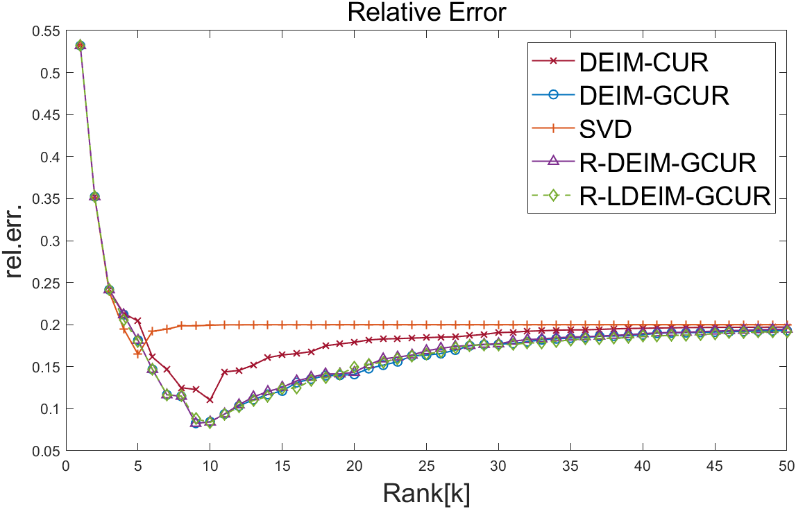
(a) $\varepsilon=0.2$

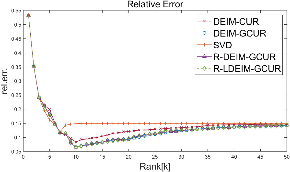
(b) $\varepsilon=0.15$

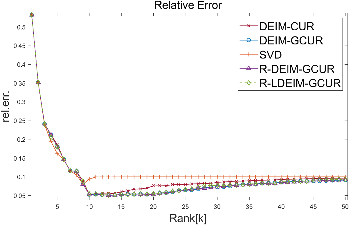
(c) $\varepsilon=0.1$

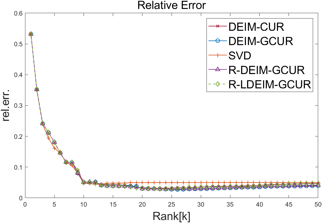
(d) $\varepsilon=0.05$

Figure 1: This figure depicts the accuracy comparison of R-GCUR approximations against the DEIM-CUR approximation and the GCUR decomposition in the recovery matrix $A$. The relative errors are shown as a function of rank $k$ for varying values of $\varepsilon$: $0.2$, $0.15$, 0.1, and $0.05$.

Table 1: Comparison of GCUR and randomized algorithms (R-DEIM-GCUR and R-LDEIM-GCUR) in CPU and relative error as the dimension and the target rank $k$ increase, with noise level $\varepsilon=0.2$.

$(m,n,k)$ $(10000,200,20)$ $(50000,200,20)$ $(100000,500,30)$ $(200000,1000,40)$ GCUR Err $0.15725$ $0.14842$ $0.18058$ $0.17292$ CPU $0.10197$ $0.54697$ $5.4971$ $40.001$ R-DEIM-GCUR Err $0.14524$ $0.16584$ $0.18260$ $0.17772$ CPU $0.027867$ $0.11137$ $0.49037$ $2.4217$ R-LDEIM-GCUR Err $0.16173$ $0.14640$ $0.16955$ $0.16758$ CPU $0.018809$ $0.056930$ $0.28019$ $1.5563$

Table 2: Comparison of GCUR and randomized algorithms (R-DEIM-GCUR and R-LDEIM-GCUR) in CPU and relative error as the dimension and the target rank $k$ increase, with noise level $\varepsilon=0.1$.

$(m,n,k)$ $(10000,1000,30)$ $(100000,500,30)$ $(200000,1000,40)$ $(200000,1000,50)$ GCUR Err $0.16493$ $0.18058$ $0.17292$ $0.18699$ CPU $2.1302$ $4.5977$ $33.783$ $51.365$ R-DEIM-GCUR Err $0.16524$ $0.18260$ $0.17772$ $0.18614$ CPU $0.56099$ $0.47876$ $2.0406$ $3.7259$ R-LDEIM-GCUR Err $0.16906$ $0.16955$ $0.16758$ $0.172631$ CPU $0.50487$ $0.27769$ $1.2856$ $1.5229$

Table 3: Comparison of GCUR and randomized algorithms (R-DEIM-GCUR and R-LDEIM-GCUR) in CPU and relative error as the dimension and the target rank $k$ increase, with noise level $\varepsilon=0.05$.

$(m,n,k)$ $(10000,500,20)$ $(100000,500,30)$ $(150000,1000,40)$ $(200000,1000,50)$ GCUR Err $0.13828$ $0.18058$ $0.18230$ $0.18699$ CPU $0.56859$ $4.5496$ $25.523$ $32.360$ R-DEIM-GCUR Err $0.13089$ $0.18260$ $0.17513$ $0.18614$ CPU $0.10336$ $0.48947$ $1.8595$ $2.6152$ R-LDEIM-GCUR Err $0.13807$ $0.16955$ $0.17975$ $0.17263$ CPU $0.079551$ $0.28887$ $1.0581$ $1.4994$

$\mathbf{Example}$ $\mathbf{5.2}$ This experiment evaluates the performance of our randomized algorithms using synthetic data sets. These data sets are generated based on the procedures described in [16, Example 5.3] and [1], which provide valuable insights into scenarios where the CUR and GCUR techniques effectively address the issue of subgroups. Our task is to reduce the dimension of target data set $A$, which contains $4m$ data points in a $3d$-dimensional feature space with four different subgroups. Each of these subgroups has distinct variances and means, and their detailed characteristics are summarized in Figure 2.

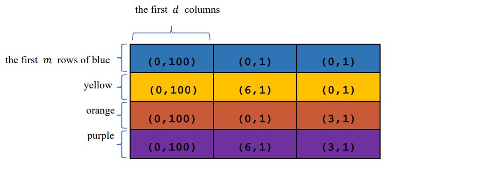
Figure 2: The $4m\times 3d$ data set $A$ contains four subgroups, and each group has $m$ data points with different mean and variance. The blocks labeled $(a,b)$ denote that it is sampled from a normal distribution with a mean of $a$ and a variance of $b$.

Usually, this task can be accomplished by the principal component analysis based on SVD, but this method fails due to the variation along the first $d$ columns of the target data set is significantly larger than in any other direction. [16, Example 5.3] demonstrates that contrastive principal component analysis (cPCA)[1] can effectively solve this problem, which identifies low-dimensional space that is enriched in a dataset relative to comparison data. Specifically, following the operations in [16], we construct the background data set $B$, which is drawn from a normal distribution, and the variance and mean of the first $d$ columns, columns $d+1$ to $2d$, and the last $d$ columns of $B$ are $100,9,1$ and $0,0,0$, respectively. Then we can extract characteristics for clustering the subgroups in $A$ by optimizing the variance of $A$ while minimizing that of $B$, which leads to a trace ratio maximization problem [12]

$$\widehat{U}=\underset{U\in\mathbb{R}^{3d\times k},U^{\mathrm{T}}U=I_{k}}{\operatorname{argmax}}\operatorname{Tr}\left[\left(U^{T}B^{T}BU\right)^{-1}\left(U^{T}A^{T}AU\right)\right].$$

In this experiment, we set $m=2500$, $d=200$.

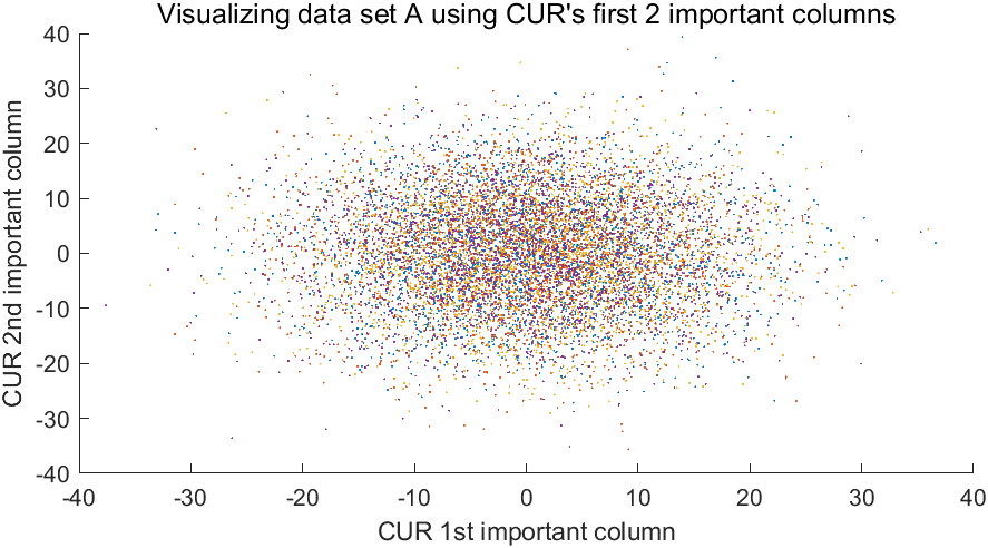
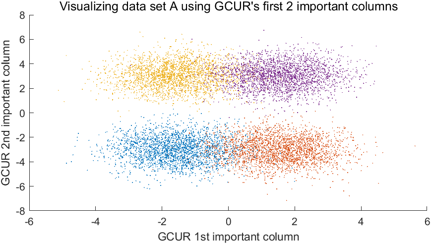
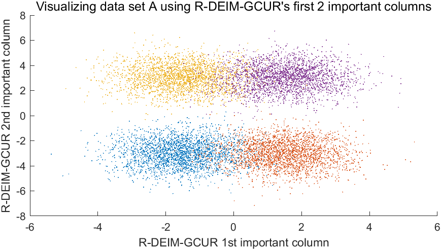
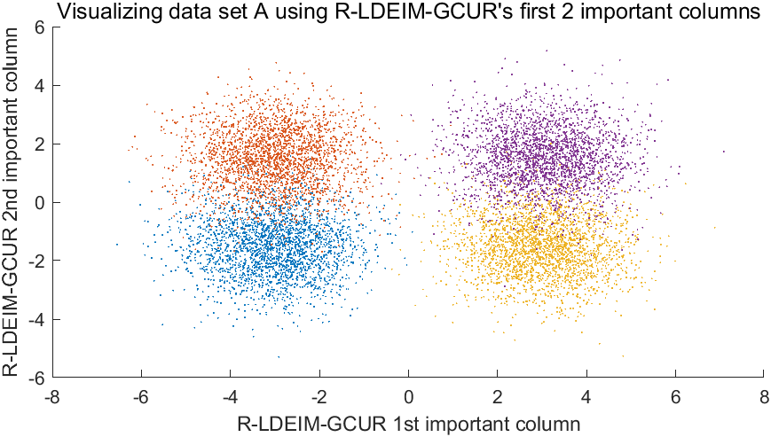
Figure 3: In the top figure, we visualize the data using the first two columns selected by CUR (left) and GCUR (right), respectively. In the bottom figure, we visualize the data using the first two columns selected by the R-DEIM-GCUR (left) and R-LDEIM-GCUR (right). In this experiment, we set $m=2500$, $d=200$ and $k=30$. The input oversampling parameters for the R-DEIM-GCUR and R-LDEIM-GCUR are set to be $70$ and $100$, respectively, and $\widehat{k}=k/2$.

Figure 3 is a visualization of the data using the first two important columns selected using the algorithms DEIM-CUR, GCUR, R-DEIM-GCUR and R-LDEM-GCUR for two of input matrix dimensions, respectively. It can be seen that the GCUR and R-GCUR methods produce a much clearer subgroup separation than the CUR. To a large extent, the GCUR and R-GCUR are able to differentiate the subgroups, while the CUR fails to do so. In terms of the running time, the nonrandom GCUR costs $1.4250$ seconds while the R-DEIM-GCUR and R-LDEIM-GCUR spend $0.83059$ seconds and $0.82679$ seconds.

For further investigation, we emulate the manipulations in [16] by comparing the performance of three subset selection methods: DEIM-CUR on $A$, GCUR, and R-GCUR on the matrix pair $(A,B)$, in identifying the subgroups of $A$. We accomplish this by selecting a subset of the columns of $A$ and comparing the classification results of each method. To evaluate the effectiveness of each method, we perform a 10-fold cross-validation [25, p. 181] and apply the ECOC (Error-Correcting Output Codes) [13] and classification tree [3] as the classifiers on the reduced data set, using the functions $\mathtt{fitcecoc}$ and $\mathtt{fitctree}$ with default parameters in MATLAB. Our results, presented in Table 4, demonstrate that the R-LDEIM-GCUR method achieves the lowest classification error rate using both the ECOC and tree classifiers, while the standard DEIM-CUR method performs the worst.

Table 4: k-Fold loss is the average classification loss overall 10-fold using CUR, GCUR, and R-GCUR as dimension reduction. The second and third columns give dimension information $m_{1}=2500$, $d_{1}=200$, $m_{2}=3000$, $d_{2}=200$, and the information on the number of columns $k=30$, selected from the data set using GCUR and R-GCUR for the ECOC classifier, likewise for the fifth and sixth columns for the tree classifier.

Method	$k$-Fold Loss		Method	$k$-Fold Loss
	($m_{1},d_{1}$)	($m_{2},d_{2}$)		($m_{1},d_{1}$)	($m_{2},d_{2}$)
CUR+ECOC	$0.7512$	$0.7521$	CUR+Tree	$0.7488$	$0.7465$
GCUR+ECOC	$0.0669$	$0.0666$	GCUR+Tree	$0.0986$	$0.09758$
R-DEIM-GCUR+ECOC	$0.06930$	$0.06700$	R-DEIM-GCUR+Tree	$0.1000$	$0.09558$
R-LDEIM-GCUR+ECOC	$0.06680$	$0.06358$	R-LDEIM-GCUR+Tree	$0.0980$	$0.09691$

$\mathbf{Example}$ $\mathbf{5.3}$ This experiment is adapted from [16, Experiment 5.4]. In this study, we evaluate the performance of R-GCUR, GCUR, and CUR on public data sets. Specifically, we analyze single-cell RNA expression levels of bone marrow mononuclear cells (BMMCs) obtained from an acute myeloid leukemia (AML) patient and two healthy individuals. The data sets are processed as in [5], retaining the 1000 most variable genes across all 16856 cells, which includes 4501 cells of the patient-035, 1985 cells, and the other of 2472 cells of the two healthy individuals. By the operation in [16], we construct the $4457\times 1000$ sparse background data matrix from the two healthy patients, containing $1,496,229$ non-zeros entries, and the target data matrix from patient-035, which has $1,628,174$ non-zeros entries. Our objective is to investigate the ability of CUR, GCUR, and R-GCUR to capture the biologically meaningful information related to the AML patient’s BMMC cells pre- and post-transplant. As depicted in Figure 4, the GCUR and R-GCUR produce nearly linearly separable clusters that correspond to pre- and post-treatment cells. The R-DEIM-GCUR and R-LDEIM-GCUR outperform GCUR in terms of running time due to their significantly lower computational cost. Notably, the running time of the nonrandom GCUR algorithm is roughly twice that of our randomized algorithms. Importantly, all methods successfully capture biologically meaningful information, effectively separating the pre- and post-transplant cell samples.

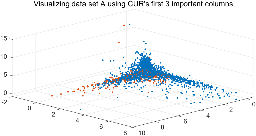
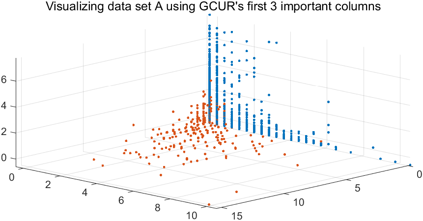
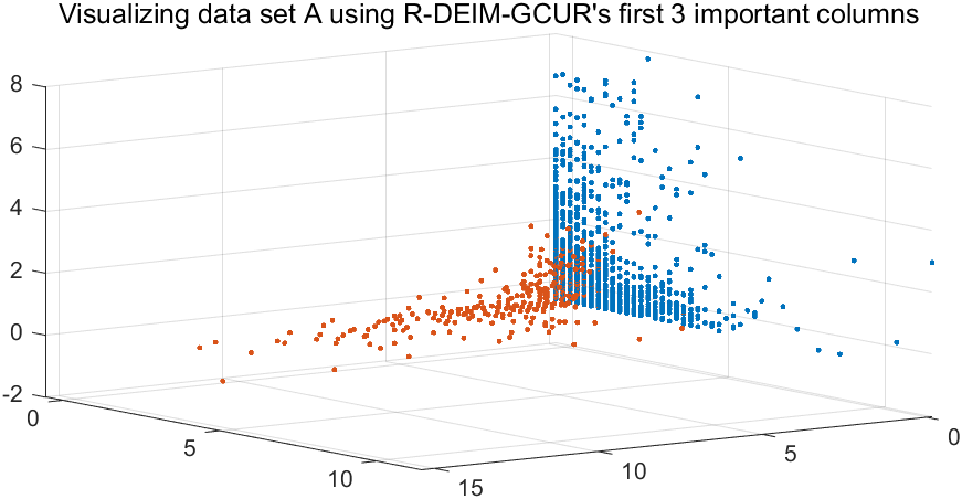
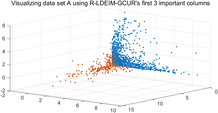
Figure 4: Acute myeloid leukemia patient-035 scRNA-seq data. In the top figure, we visualize the data using the first three genes selected by DEIM-CUR (top-left) and GCUR (top-right), and the CUR does not effectively give a discernible cluster of the pre- and post transplant cells. In the bottom figure, we visualize the data using the first three genes selected by R-DEIM-GCUR (bottom-left) and R-LDEIM-GCUR (bottom-right), which both produce almost linearly separable clusters which correspond to pre- and posttreatment cells.

$\mathbf{Example}$ $\mathbf{5.4}$ This experiment demonstrates the performance of our randomized algorithm for producing the RSVD-CUR decomposition. This test is an adaptation of [18, Experiment 1], which considers a matrix perturbation problem of the form $A_{E}=A+BFG$, where $A\in\mathbb{R}^{m\times n}$, matrices $B\in\mathbb{R}^{m\times l}$, $G\in\mathbb{R}^{d\times n}$ are noises distributed normally with mean $0$ and unit variance, and our goal is to reconstruct a low-rank matrix $A$ from $A_{E}$. We evaluate and compare a rank-$k$ RSVD-CUR decomposition of $A_{E}$, obtained by the nonrandom RSVD-CUR algorithm and its counterpart randomized algorithm, in terms of reconstructing matrix $A$ and the running time. The approximation quality of the decomposition is assessed by the relative matrix approximation error, i.e., $\mathrm{Err}=\|A-\widetilde{A}\|/\|A\|$, where $\widetilde{A}$ is the reconstructed low-rank matrix. As an adaptation of the experiment in [34, Example 1] and [18, Experiment 1], we generate a rank-$100$ sparse nonnegative matrix $A\in\mathbb{R}^{m\times n}$ of the form

$$A=\sum_{j=1}^{10}\frac{2}{j}\mathbf{x}_{j}\mathbf{y}_{j}^{\mathrm{T}}+\sum_{j=11}^{100}\frac{1}{j}\mathbf{x}_{j}\mathbf{y}_{j}^{\mathrm{T}}$$

where $\mathbf{x}_{j}\in\mathbb{R}^{m}$ and $\mathbf{x}_{j}\in\mathbb{R}^{n}$ are random sparse vectors with nonnegative entries. We then perturb $A$ with a nonwhite noise matrix $BFG$ [21]. The resulting perturbed matrix we use is of the form

$$A_{E}=A+\varepsilon\frac{\|A\|}{\|BFG\|}BFG,$$

where $\varepsilon$ is the noise level. Given each noise level $\varepsilon\in\{0.1,0.15,0.2\}$, we generate the RSVD-CUR decomposition computed by the RSVD-CUR algorithms and the randomized algorithm for varying dimensions and the target rank $k$ values. Here we set the parameter $\widehat{k}$, contained in the L-DEIM to be $\widehat{k}=k/2$ and $\widehat{k}=k$, respectively. The corresponding results are displayed in Tables 5, 6 and 7, where we can see that the randomized algorithms give comparable relative errors at substantially less cost. It indicates that using the random sampling techniques and L-DEIM method leads to a dramatic speed-up over classical approaches.

Table 5: Comparison of RSVD-CUR and randomized algorithms in CPU and relative error as the dimension $l$, $d$, $m$, $n$ ( we set $m=n$) and the target rank $k$ increase, with noise level $\varepsilon=0.1$.

$(l,d,m,k)$			$(1000,500,100,10)$	$(5000,1000,100,20)$	$(7000,2000,200,30)$
DEIM-RSVD-CUR		Err	$0.095573$	$0.085198$	$0.084425$
		CPU	$0.099726$	$8.1768$	$15.251$
LDEIM-RSVD-CUR		Err	$0.11652$	$0.094442$	$0.083729$
		CPU	$0.098987$	$8.5575$	$15.886$
oversampling parameter			$80$	$500$	$500$
R-LDEIM-RSVD-CUR	$k=\widehat{k}$	Err	$0.095573$	$0.085198$	$0.084425$
		CPU	$0.028330$	$0.057914$	$0.39295$
	$\widehat{k}=k/2$	Err	$0.095573$	$0.085198$	$0.084425$
		CPU	$0.024517$	$0.056423$	$0.50397$

Table 6: Comparison of RSVD-CUR and randomized algorithms in CPU and relative error as the dimension $l$, $d$, $m$, $n$ ( we set $m=n$) and the target rank $k$ increase, with noise level $\varepsilon=0.15$.

$(l,d,m,k)$			$(5000,1000,200,20)$	$(10000,2000,500,30)$	$(20000,2000,500,40)$
DEIM-RSVD-CUR		Err	$0.13123$	$0.15709$	$0.14705$
		CPU	$7.5313$	$62.594$	$328.99$
LDEIM-RSVD-CUR		Err	$0.13103$	$0.16492$	$0.15604$
		CPU	$7.3077$	$61.396$	$330.20$
oversampling parameter			$500$	$500$	$500$
R-LDEIM-RSVD-CUR	$k=\widehat{k}$	Err	$0.13123$	$0.15709$	$0.14705$
		CPU	$0.33164$	$3.0591$	$2.7742$
	$\widehat{k}=k/2$	Err	$0.13123$	$0.15709$	$0.14705$
		CPU	$0.34972$	$2.5485$	$2.9289$

Table 7: Comparison of RSVD-CUR and randomized algorithms in CPU and relative error as the dimension $l$, $d$, $m$, $n$ ( we set $m=n$) and the target rank $k$ increase, with noise level $\varepsilon=0.2$.

$(l,d,m,k)$			$(5000,1000,100,10)$	$(10000,1000,500,30)$	$(7000,2000,200,30)$
DEIM-RSVD-CUR		Err	$0.15325$	$0.18345$	$0.18429$
		CPU	$7.9139$	$56.001$	$384.17$
LDEIM-RSVD-CUR		Err	$0.14943$	$0.21517$	$0.19300$
		CPU	$7.9627$	$51.571$	$357.91$
oversampling parameter			$100$	$500$	$500$
R-LDEIM-RSVD-CUR	$k=\widehat{k}$	Err	$0.15325$	$0.18345$	$0.18429$
		CPU	$0.079395$	$2.1681$	$3.9116$
	$\widehat{k}=k/2$	Err	$0.15325$	$0.18345$	$0.18429$
		CPU	$0.06830$	$2.0079$	$3.8923$

6 Conclusion

In this paper, by combining the random sampling techniques with the L-DEIM method, we develop new efficient randomized algorithms for computing the GCUR decomposition for matrix pairs and the RSVD-CUR decomposition for matrix triplets with a given target rank. We also provided the detailed probabilistic analysis for the proposed randomized algorithms. Theoretical analyses and numerical examples illustrate that exploiting the randomized techniques results in a significant improvement in terms of the CPU time while keeping a high degree of accuracy. Finally, it is natural to consider applying the L-DEIM for developing randomized algorithms that adaptively find a low-rank representation satisfying a given tolerance, which is beneficial when the target rank is not known in advance, and it will be discussed in our future work.

Funding

Z. Cao is supported by the National Natural Science Foundation of China under Grant 11801534. Y. Wei is supported by the National Natural Science Foundation of China under Grant 12271108 and the Innovation Program of Shanghai Municipal Education Committee. P. Xie is supported by the National Natural Science Foundation of China under Grants 12271108, 11801534 and the Fundamental Research Funds for the Central Universities under Grant 202264006.

Declarations

The authors have not disclosed any competing interests.

Data Availability Statements

All datasets are publicly available.

References

• [1] A. Abid, M. J. Zhang, V. K. Bagaria, and J. Zou, Exploring patterns enriched in a dataset with contrastive principal component analysis, Nature Communications, 9 (2018), pp. 1–7.
• [2] Z. Bai and J. W. Demmel, Computing the generalized singular value decomposition, SIAM Journal on Scientific Computing, 14 (1993), pp. 1464–1486.
• [3] R. E. Banfield, L. O. Hall, K. W. Bowyer, and W. P. Kegelmeyer, A comparison of decision tree ensemble creation techniques, IEEE Transactions on Pattern Analysis and Machine Intelligence, 29 (2006), pp. 173–180.
• [4] M. Barrault, Y. Maday, N. C. Nguyen, and A. T. Patera, An ‘empirical interpolation’ method: application to efficient reduced-basis discretization of partial differential equations, Comptes Rendus Mathematique, 339 (2004), pp. 667–672.
• [5] P. Boileau, N. S. Hejazi, and S. Dudoit, Exploring high-dimensional biological data with sparse contrastive principal component analysis, Bioinformatics, 36 (2020), pp. 3422–3430.
• [6] C. Boutsidis and P. Drineas, Random projections for the nonnegative least-squares problem, Linear Algebra and Its Applications, 431 (2009), pp. 760–771.
• [7] C. Boutsidis and D. P. Woodruff, Optimal CUR matrix decompositions, in Proceedings of the forty-sixth annual ACM symposium on Theory of computing, 2014, pp. 353–362.
• [8] H. Cai, K. Hamm, L. Huang, J. Li, and T. Wang, Rapid robust principal component analysis: CUR accelerated inexact low rank estimation, IEEE Signal Processing Letters, 28 (2020), pp. 116–120.
• [9] H. Cai, K. Hamm, L. Huang, and D. Needell, Robust CUR decomposition: Theory and imaging applications, SIAM Journal on Imaging Sciences, 14 (2021), pp. 1472–1503.
• [10] H. Cai, L. Huang, P. Li, and D. Needell, Matrix completion with cross-concentrated sampling: Bridging uniform sampling and CUR sampling, arXiv:2208.09723, (2022).
• [11] S. Chaturantabut and D. C. Sorensen, Nonlinear model reduction via discrete empirical interpolation, SIAM Journal on Scientific Computing, 32 (2010), pp. 2737–2764.
• [12] J. Chen, G. Wang, and G. B. Giannakis, Nonlinear dimensionality reduction for discriminative analytics of multiple datasets, IEEE Transactions on Signal Processing, 67 (2018), pp. 740–752.
• [13] D. Chu, L. De Lathauwer, and B. De Moor, On the computation of the restricted singular value decomposition via the cosine-sine decomposition, SIAM Journal on Matrix Analysis and Applications, 22 (2000), pp. 580–601.
• [14] B. L. De Moor and G. H. Golub, The restricted singular value decomposition: properties and applications, SIAM Journal on Matrix Analysis and Applications, 12 (1991), pp. 401–425.
• [15] P. Drineas, M. W. Mahoney, and S. Muthukrishnan, Relative-error CUR matrix decompositions, SIAM Journal on Matrix Analysis and Applications, 30 (2008), pp. 844–881.
• [16] P. Y. Gidisu and M. E. Hochstenbach, A generalized CUR decomposition for matrix pairs, SIAM Journal on Mathematics of Data Science, 4 (2022), pp. 386–409.
• [17] P. Y. Gidisu and M. E. Hochstenbach, A hybrid DEIM and leverage scores based method for CUR index selection, Progress in Industrial Mathematics at ECMI 2021, (2022), pp. 147–153.
• [18]  , A Restricted SVD type CUR decomposition for matrix triplets, arXiv:2204.02113, (2022).
• [19] N. Halko, P.-G. Martinsson, and J. A. Tropp, Finding structure with randomness: Probabilistic algorithms for constructing approximate matrix decompositions, SIAM Review, 53 (2011), pp. 217–288.
• [20] K. Hamm and L. Huang, Perturbations of CUR decompositions, SIAM Journal on Matrix Analysis and Applications, 42 (2021), pp. 351–375.
• [21] P. C. Hansen, Rank-Deficient and Discrete Ill-Posed Problems, Society for Industrial and Applied Mathematics, Philadelphia, PA, 1998.
• [22] E. P. Hendryx, B. M. Rivière, and C. G. Rusin, An extended DEIM algorithm for subset selection and class identification, Machine Learning, 110 (2021), pp. 621–650.
• [23] R. A. Horn and C. R. Johnson, Topics in Matrix Analysis, Cambridge University Press, Cambridge, 1991.
• [24] J. Huang and Z. Jia, Two harmonic Jacobi-Davidson methods for computing a partial generalized singular value decomposition of a large matrix pair, Journal of Scientific Computing, 93 (2022). Article number: 41.
• [25] G. James, D. Witten, T. Hastie, and R. Tibshirani, An introduction to statistical learning, vol. 112, Springer, 2013.
• [26] I. T. Jolliffe, Discarding variables in a principal component analysis. i: Artificial data, Journal of the Royal Statistical Society: Series C (Applied Statistics), 21 (1972), pp. 160–173.
• [27] R.-C. Li, Bounds on perturbations of generalized singular values and of associated subspaces, SIAM Journal on Matrix Analysis and Applications, 14 (1993), pp. 195–234.
• [28] M. W. Mahoney and P. Drineas, CUR matrix decompositions for improved data analysis, Proceedings of the National Academy of Sciences, 106 (2009), pp. 697–702.
• [29] C. C. Paige and M. A. Saunders, Towards a generalized singular value decomposition, SIAM Journal on Numerical Analysis, 18 (1981), pp. 398–405.
• [30] D. Papailiopoulos, A. Kyrillidis, and C. Boutsidis, Provable deterministic leverage score sampling, in Proceedings of the 20th ACM SIGKDD International Conference on Knowledge Discovery and Data Mining, 2014, pp. 997–1006.
• [31] D. Rachkovskij and E. Revunova, A randomized method for solving discrete ill-posed problems, Cybernetics and Systems Analysis, 48 (2012), pp. 621–635.
• [32] A. K. Saibaba, J. Hart, and B. van Bloemen Waanders, Randomized algorithms for generalized singular value decomposition with application to sensitivity analysis, Numerical Linear Algebra with Applications, 28 (2021). pp. e2364.
• [33] A. K. Saibaba, J. Lee, and P. K. Kitanidis, Randomized algorithms for generalized hermitian eigenvalue problems with application to computing Karhunen–Loève expansion, Numerical Linear Algebra with Applications, 23 (2016), pp. 314–339.
• [34] D. C. Sorensen and M. Embree, A DEIM induced CUR factorization, SIAM Journal on Scientific Computing, 38 (2016), pp. A1454–A1482.
• [35] G. Stewart, Computing the CS decomposition of a partitioned orthonormal matrix, Numerische Mathematik, 40 (1982), pp. 297–306.
• [36] G. W. Stewart, Four algorithms for the the efficient computation of truncated pivoted QR approximations to a sparse matrix, Numerische Mathematik, 83 (1999), pp. 313–323.
• [37] J. G. Sun, On the perturbation of generalized singular values, Math. Numer. Sinica, 4 (1982), pp. 229–233.
• [38] J.-G. Sun, Perturbation analysis for the generalized singular value problem, SIAM Journal on Numerical Analysis, 20 (1983), pp. 611–625.
• [39] D. B. Szyld, The many proofs of an identity on the norm of oblique projections, Numerical Algorithms, 42 (2006), pp. 309–323.
• [40] C. F. Van Loan, Generalizing the singular value decomposition, SIAM Journal on Numerical Analysis, 13 (1976), pp. 76–83.
• [41] C. F. Van Loan, Computing the CS and the generalized singular value decompositions, Numerische Mathematik, 46 (1985), pp. 479–491.
• [42] S. Voronin and P.-G. Martinsson, A CUR factorization algorithm based on the interpolative decomposition, arXiv:1412.8447, (2014).
• [43] S. Wang and Z. Zhang, Improving CUR matrix decomposition and the Nyström approximation via adaptive sampling, The Journal of Machine Learning Research, 14 (2013), pp. 2729–2769.
• [44] W. Wei, H. Zhang, X. Yang, and X. Chen, Randomized generalized singular value decomposition, Communications on Applied Mathematics and Computation, 3 (2021), pp. 137–156.
• [45] Y. Wei, P. Stanimirović, and M. Petković, Numerical and Symbolic Computations of Ggeneralized Inverses, Hackensack, NJ: World Scientific, 2018.
• [46] Y. Wei, P. Xie, and L. Zhang, Tikhonov regularization and randomized GSVD, SIAM Journal on Matrix Analysis and Applications, 37 (2016), pp. 649–675.
• [47] H. Xiang and J. Zou, Regularization with randomized SVD for large-scale discrete inverse problems, Inverse Problems, 29 (2013). Paper No. 085008.
• [48] P. Xie, H. Xiang, and Y. Wei, Randomized algorithms for total least squares problems, Numerical Linear Algebra with Applications, 26 (2019). e2219.
• [49] C. Xu, D. Tao, and C. Xu, A survey on multi-view learning, arXiv:1304.5634, (2013).
• [50] H. Zha, The restricted singular value decomposition of matrix triplets, SIAM Journal on Matrix Analysis and Applications, 12 (1991), pp. 172–194.
• [51]  , Computing the generalized singular values/vectors of large sparse or structured matrix pairs, Numerische Mathematik, 72 (1996), pp. 391–417.
• [52] L. Zhang and Y. Wei, Randomized core reduction for discrete ill-posed problem, Journal of Computational and Applied Mathematics, 375 (2020). Paper No. 112797.
• [53] L. Zhang, Y. Wei, and E. K.-w. Chu, Neural network for computing GSVD and RSVD, Neurocomputing, 444 (2021), pp. 59–66.
• [54] I. N. Zwaan, Towards a more robust algorithm for computing the restricted singular value decomposition, arXiv:2002.04828, (2020).