Spectral properties of the Laplacian of temporal networks following a constant block Jacobi model

Abstract

We study the behavior of the eigenvectors associated with the smallest eigenvalues of the Laplacian matrix of temporal networks. We consider the multilayer representation of temporal networks, i.e. a set of networks linked through ordinal interconnected layers. We analyze the Laplacian matrix, known as supra-Laplacian, constructed through the supra-adjacency matrix associated with the multilayer formulation of temporal networks, using a constant block Jacobi model which has closed-form solution. To do this, we assume that the inter-layer weights are perturbations of the Kronecker sum of the separate adjacency matrices forming the temporal network. Thus we investigate the properties of the eigenvectors associated with the smallest eigenvalues (close to zero) of the supra-Laplacian matrix. Using arguments of perturbation theory, we show that these eigenvectors can be approximated by linear combinations of the zero eigenvectors of the individual time layers. This finding is crucial in reconsidering and generalizing the role of the Fielder vector in supra-Laplacian matrices.

1 Introduction

In recent years, one of the major lines of research in complex network analysis is the topological changes that occur in a network over time. A sequence of networks with such a time-varying nature can be formalized as a temporal network Holme and Saramäki (2012). The multilayer formulation of temporal networks Kivelä et al. (2014) is one way to consider the interconnected topological structure changing over time: ordinal interconnections between layers determine how a given node in one layer and its given counterparts in the previous and next time point layers are linked and influence each other. The network analysis community has strong traditions in using the spectral properties Moreno and Arenas (2013); Sol et al. (2013) of multilayer networks for various purposes such as centrality measures De Domenico et al. (2016) or investigating diffusion processes Sol et al. (2013).

One challenge associated with understanding the spectral properties of the temporal networks is the lack of available tools that respect the fundamental distinction between within-layer and inter-layer edges Kivelä et al. (2014); Taylor et al. (2015); De Domenico et al. (2013) when studying the spectral properties of the Laplacian matrix $\mathcal{L}$ of temporal networks, known as supra-Laplacian. A number of investigations were undertaken to show that the inter-layer couplings in multilayer networks distort those spectral properties and to explain the effect of different inter-layer weights over the eigenvalues of the supra-Laplacian Moreno and Arenas (2013); Sol et al. (2013). Up to our knowledge, there is no work related to the understanding of the information carried by the eigenvectors corresponding to the smallest eignevalues of the supra-Laplacian.

The spectral analysis on a network is nowadays understood as studying the spectral properties of the various Laplacian matrices defined on the network. In particular, for the so-called normalized Laplacian the most interesting are usually the smallest eigenvalues and their eigenvectors.

For a Laplacian matrix, the eigenvector corresponding to the smallest eigenvalue, $\lambda_{1}=0$, is constant or weighted by the node degrees if the Laplacian is normalized Chung (1996). The eigenvector corresponding to the smallest non-zero eigenvalue, known as the algebraic connectivity, is in practice used for partitioning purposes Luo et al. (2002); Luxburg (2007) and is known as the Fiedler vector. In this article, we consider slowly-changing temporal networks which means that the adjacency matrices forming the different time layers change relatively slowly Enright and Kao (2018). The main objective of the present paper is to draw a maximal profit of this important property for the majority of temporal networks. In particular, for every temporal network, for a sufficiently small interval, we have this effect.

Further, we add inter-layer weights to the temporal network which may be considered as perturbations of the Kronecker sum of the separate adjacency matrices forming the different time layers, and we consider the Laplacian of the resulting matrix which is usually called supra-Laplacian Kivelä et al. (2014). This point of view on the temporal networks, allows us to find an approximate closed form solution of the eigenvectors corresponding to the smallest eigenvalues of the supra-Laplacian. In particular, by applying arguments from perturbation theory, we are able to show that the eigenvectors corresponding to the smallest eigenvalues (of the supra-Laplacian) are well approximated by the space of the perturbed eigenvectors corresponding to all zero eigenvalues of the Laplacian matrices corresponding to the networks of the separate time layers.

The paper is organised as follows: in Sec. 2, we present the construction of the temporal network following a constant block Jacobi model. This model appears in a natural way as a first order approximation to the slowly-changing temporal network, and enjoys a closed-form solution of the eigenvectors of the supra-Laplacian matrix; in Sec. 3 we investigate the spectral properties of the supra-Laplacian and obtain an eigenvector solution of the reduced system; Sec. 4 is devoted to identifying the smallest eigenvectors, which are obtained by perturbation of the zero eigenvectors of the separate time layers, and discussing the influence of density and number of layers on these eigenvectors; finally we state the conclusions.

2 Temporal network following constant block Jacobi model: notations and definitions

A temporal network is a set of networks in which edges and nodes vary in time. In this work, we make the assumption that each node $i$ is present in all layers. We use the notation $G^{t}$ for a layer in an ordered sequence of $T$ networks $\mathcal{T}=\left\{G^{1},G^{2},...,G^{T}\right\}$ with $G^{t}=\left(V,A^{t}\right)$ where $t\in\left\{1,2,...,T\right\}$ and the number of nodes is $N,$ i.e. $N=\left|V\right|.$ Here $A^{t}$ is a binary undirected and connected adjacency matrix. In order to use the multilayer framework for representing a temporal network, we consider the diagonal ordinal coupling of layers Kivelä et al. (2014); Bassett et al. (2011); Mucha et al. (2010), to define a new supra-network $\widetilde{\mathcal{T}}$ . We define the coupling edges: we denote by $\omega_{i}^{t,p}\in\mathbb{R}$ the value of the inter-layer edge weight between node $i$ in different time layers $t$ and $p$. Our main assumption is that only neighbouring layers may be connected, i.e. $\omega_{i}^{t,p}=0$ for all layers $G^{t}$ and $G^{p}$, with $p\neq t-1$ and $p\neq t+1$. No other edges between $G^{t}$ and $G^{p}$ exist for indices $t\neq p.$

As a result, the multilayer framework of the temporal network is expressed in an $NT$-node single adjacency matrix $\mathcal{A}$ of size $NT\times NT$ which is simply the adjacency matrix of the network $\widetilde{\mathcal{T}}$ , referred to as supra-adjacency matrix. Clearly, the diagonal blocks of $\mathcal{A}$ are the adjacency matrices $A^{t}$, and the off-diagonal blocks are the inter-layer weight matrices $W^{t,p}=diag(\omega_{1}^{t,p},\omega_{2}^{t,p},...,\omega_{N}^{t,p})$ if $p=t-1$ or $p=t+1.$

The usual within-layer degree of node $i$ in layer $G^{t}$ is defined as $d_{i}^{t}:={\sum_{j=1}^{N}}A_{ij}^{t}$ while the multilayer node degree of node $i$ in layer $G^{t}$ is $\mathfrak{d}_{i}^{t}:=d_{i}^{t}+\omega_{i}^{t,t-1}+\omega_{i}^{t,t+1}$. Define the degree matrix $\mathcal{D}$ as $\mathcal{D}:=\text{diag}\left(\mathfrak{d}_{1}^{1},\mathfrak{d}_{2}^{1},...,\mathfrak{d}_{N}^{1},\mathfrak{d}_{1}^{2},...,\mathfrak{d}_{N}^{2},...,\mathfrak{d}_{N}^{T}\right)$. The normalized supra-Laplacian $\mathcal{L}$ is defined as $\mathcal{L}:\mathfrak{=}\mathcal{D}^{-\frac{1}{2}}\left(\mathcal{D-A}\right)\mathcal{D}^{-\frac{1}{2}}$ Chung (1996).

The supra-adjacency matrix $\mathcal{A}^{0}$ with $0$ inter-layer weights and its corresponding Laplacian matrix $\mathcal{L}^{0}$ are directly expressed as a Kronecker sum:

$$\mathcal{A}^{0}:=\oplus_{t=1}^{T}A^{t}\longrightarrow\mathcal{L}^{0}=\oplus_{t=1}^{T}L^{t}$$ (1)

where $L^{t}$ is the normalized Laplacian of network $G^{t}.$

From spectral graph theory Chung (1996), we know that due to the connectedness of $A^{t},$ for every time point $t$ the solution to $L^{t}v_{1}^{t}=0$ corresponds to the first eigenvalue $\lambda_{1}^{t}=0$ which has multiplicity one and the corresponding eigenvector $v_{1}$ is the eigenvector $(D^{t})^{\frac{1}{2}}\boldsymbol{1}$, where $\boldsymbol{1}$ is the constant one vector and $D^{t}$ is the degree matrix for the adjacency matrix $A^{t}$.

Hence, the equation $\mathcal{L}^{0}v=0$ has a $T-$dimensional subspace of solutions and we find its basis explicitly: namely, for every $t$ we define the column vector $V^{t}\in\mathbb{R}^{NT},$ as a zero-padded vector with $v_{1}^{t}$ at the position of the $t^{th}$ block. Thus, all solutions to $\mathcal{L}^{0}v=0$ are given by $v=\sum_{t=1}^{T}\alpha_{t}V^{t}$ for arbitrary constants $\alpha_{t}$.

The main objective of the present paper is to consider an ideal case of a temporal network which is slowly-changing in time, hence, is well approximated by a temporal network following a constant block Jacobi model: Let us consider the case where $A^{t}=A$ for all $t$ and $W^{t,p}=W$ for all $t,p$. An important step in our construction is to ”periodize” the temporal network, which will provide the existence of a nice closed-form solution of the resulting network. This is not a very artificial approach since the ”slowly-changing” of the network assumes that the network does not vary too much from the initial to the final layer: Namely, we construct a ”periodic” supra-adjacency matrix $\mathcal{A}$ and its corresponding supra-Laplacian matrix $\mathcal{L}$ for temporal networks, by including non-zero diagonal blocks on the upper-right and lower-left corner blocks. In other words, we include inter-layer weights between the first time layer $A^{1}$ and the last time layer $A^{T}$. The resulting matrix $\mathcal{A}$ is a periodic constant block Jacobi matrix which gives the name of the model. In view of the slowly-changing nature of the temporal network $G^{t},$ the matrix $\mathcal{A}$ is a perturbation of the matrix $\mathcal{A}^{0}$ and $\mathcal{L}$ is a perturbation of the matrix $\mathcal{L}^{0}.$

Furtheron, the resulting supra-Laplacian matrix $\mathcal{L}$ is given by the following $T\times T$ block matrix, which may be easily proved to be an infinite periodic block Jacobi matrix Sahbani (2015):

$$\mathcal{L}:=\underset{T}{\underbrace{\left(\begin{array}[c]{ccccc}\widetilde{L}&\widetilde{L}_{W}&&&\widetilde{L}_{W}\\ \widetilde{L}_{W}&\widetilde{L}&\widetilde{L}_{W}&&\\ &\widetilde{L}_{W}&\widetilde{L}&&\\ &&&\cdot\cdot\cdot&\widetilde{L}_{W}\\ \widetilde{L}_{W}&&&\widetilde{L}_{W}&\widetilde{L}\end{array}\right)}}$$ (2)

We have to note that if we have the same $\omega$ for all matrices $W,$ then the blocks of the block-diagonal matrix $\mathcal{D}$ contain the matrices $D^{t}+2\omega I$. Since for every $t$ holds equation $L^{t}=I-D^{-1/2}AD^{-1/2},$ and since the matrix $D^{-1/2}AD^{-1/2}$ has entries $d_{i}^{-1/2}d_{j}^{-1/2}a_{ij}$, we see that $\widetilde{L}$ is a perturbation of $L$ which has just the elements $-\left(d_{i}+2\omega\right)^{-1/2}\left(d_{j}+2\omega\right)^{-1/2}a_{ij}$ and not $-d_{i}^{-1/2}d_{j}^{-1/2}a_{ij}$. Hence, written formally, we have the equality

$$\widetilde{L}=I-\left(D+2\omega I\right)^{-1/2}A\left(D+2\omega I\right)^{-1/2}$$

On the other hand, the matrix $\widetilde{L}_{W}$ is equal to $-\omega\left(D+2\omega I\right)^{-1}$ , in equation (2).

The big advantage of the constant block Jacobi model is that we can find ”explicitly” its spectrum which we discuss in the next sections.

3 Smallest eigenvalues and paired eigenvectors of the supra-Laplacian $\mathcal{L}$ of temporal networks following constant block Jacobi model

As we know from spectral graph theory Chung (1996), the eigenvalues of the Laplacian $L^{t}$ and of the supra-Laplacian $\mathcal{L}$ are non-negative, and the minimal eigenvalue is $0$, as mentioned above. As usual, in the applications the small eigenvalues and the corresponding eigenvectors are of particular importance. By perturbation theory, some of those eigenvalues which are very close to $0$ are obtained as a direct perturbation of the $0$ eigenvalues of all separate time layer Laplacian matrices $L^{t},$ and the same holds about their paired eigenvectors. On the other hand, the eigenvectors paired to the bigger eigenvalues are obtained as perturbations not only of the $0$ eigenvectors of the separate matrices $L^{t}$ but also of the Fielder (and the higher) eigenvectors of the separate matrices $L^{t}$.

The solution for the Laplacian $\mathcal{L}$ in equation (2) is defined by:

$$\mathcal{L}\psi=\lambda\psi$$ (3)

and for finding it we apply a classical technique based on discrete Fourier transforms (DFTs), see e.g. Sahbani (2015). To do this we represent each vector $\psi\in\mathbb{R}^{NT}$ as the sequence of vectors $\left[\psi_{1},\psi_{2},...,\psi_{T}\right]$ where each vector $\psi_{j}$ is the portion of eigenvector $\psi$ corresponding to the $j^{th}$ time block. Then equation (3) splits into the equations

$$\widetilde{L}_{W}\psi_{j-1}+\widetilde{L}\psi_{j}+\widetilde{L}_{W}\psi_{j+1}=\lambda\psi_{j}\qquad\text{for }j=1,2,...,T$$ (4)

where for the sake of notation simplicity we have put

$$\psi_{0}=\psi_{T},\qquad\psi_{T+1}=\psi_{1}.$$

For $k=0,1,2,...,T-1,$ we denote the DFT of vector $\psi$ at value $k$ by $\widehat{\psi}(k)\in\mathbb{R}^{N},$ and put

$$\widehat{\psi}(k):=\sum_{j=0}^{T-1}e^{-ijk\frac{2\pi}{T}}\psi_{j+1}.$$ (5)

It is important that from the set of DFT vectors $\{\widehat{\psi}\left(k\right)\}_{k=0}^{T-1}$ we may recover the whole vector $\psi\in\mathbb{R}^{NT}$ using the Fourier inversion formula:

$$\psi_{j}=\frac{1}{T}\sum_{k=0}^{T-1}\widehat{\psi}(k)e^{ijk\frac{2\pi}{T}}.$$ (6)

Now by applying the DFT (5) to equations (4) (i.e. by multiplying by exponents and summing up the equations), we obtain the fundamental equations satisfied by the DFT of the vector $\psi$ defined in formula (5):

$$\left[\widetilde{L}+2\cos\left(k\frac{2\pi}{T}\right)\widetilde{L}_{W}\right]\widehat{\psi}\left(k\right)=\lambda\widehat{\psi}\left(k\right)\hskip 2.5pt$$ (7)

for $$k=0,1,...,T-1.$$

The following theorem justifies the application of the DFTs for solving the system (3):

Theorem 1

The spectrum (with multiplicities) of the supra-Laplacian $\mathcal{L}$ in equation (2) of a temporal network following a periodic constant block Jacobi model coincides with the union of the spectra of the matrices $\widetilde{L}+2\cos\left(k\frac{2\pi}{T}\right)\widetilde{L}_{W},$ i.e.

$$spec\left(\mathcal{L}\right)=\cup_{k=0}^{T-1}spec\left(\widetilde{L}+2\cos\left(k\frac{2\pi}{T}\right)\widetilde{L}_{W}\right)$$ (8)

Proof 2

First, we prove the inclusion

$$spec\left(\mathcal{L}\right)\subseteq\cup_{k=0}^{T-1}spec\left(\widetilde{L}+2\cos\left(k\frac{2\pi}{T}\right)\widetilde{L}_{W}\right).$$

Indeed, by the above arguments, if we have an eigenvalue $\lambda$ with eigenvector $\psi$ solving system (4), then for every $k$ with $0\leq k\leq T-1$ we have equation (7), i.e.

$$\left[\widetilde{L}+2\cos\left(k\frac{2\pi}{T}\right)\widetilde{L}_{W}\right]\widehat{\psi}\left(k\right)=\lambda\widehat{\psi}\left(k\right).$$

Hence, $\lambda$ is an eigenvalue for all matrices $\widetilde{L}+2\cos\left(k\frac{2\pi}{T}\right)\widetilde{L}_{W}$ with eigenvector $\widehat{\psi}\left(k\right).$ Now, we prove the opposite inclusion:

$$\cup_{k=0}^{T-1}spec\left(\widetilde{L}+2\cos\left(k\frac{2\pi}{T}\right)\widetilde{L}_{W}\right)\subseteq spec\left(\mathcal{L}\right).$$

Assume that $\lambda^{\ast}$ is an eigenvalue with eigenvector $v^{\ast}$ for the matrix $\widetilde{L}+2\cos\left(k\frac{2\pi}{T}\right)\widetilde{L}_{W}$, i.e.

$$\left[\widetilde{L}+2\cos\left(k\frac{2\pi}{T}\right)\widetilde{L}_{W}\right]v^{\ast}=\lambda^{\ast}v^{\ast}.$$

We define the vector $\varphi\in\mathbb{R}^{NT}$ by putting

$$\varphi_{k+1} =v^{\ast}$$

$$\varphi_{m} =0\qquad\text{for }m\neq k+1,m=1,2,...,T.$$

By the inversion formula (6) we define the vector

$$\psi_{j}:=\varphi_{k+1}e^{ijk\frac{2\pi}{T}}\qquad\text{for }j=1,2,...,T.$$

We show that it satisfies the eigenvalue equation (4) since

$$\widetilde{L}_{W}\psi_{j-1}+\widetilde{L}\psi_{j}+\widetilde{L}_{W}\psi_{j+1}=\lambda^{\ast}\psi_{j}$$

i.e.

$$e^{i\left(j-1\right)k\frac{2\pi}{T}}\widetilde{L}_{W}v^{\ast}+e^{ijk\frac{2\pi}{T}}\widetilde{L}v^{\ast}+e^{i\left(j+1\right)k\frac{2\pi}{T}}\widetilde{L}_{W}v^{\ast}=\lambda^{\ast}e^{ijk\frac{2\pi}{T}}v^{\ast}$$

But the last is equivalent to equation

$$e^{-ik\frac{2\pi}{T}}\widetilde{L}_{W}v^{\ast}+\widetilde{L}v^{\ast}+e^{ik\frac{2\pi}{T}}\widetilde{L}_{W}v^{\ast}=\lambda^{\ast}v^{\ast}$$

hence, to equation $\widetilde{L}v^{\ast}+2\cos\left(k\frac{2\pi}{T}\right)\widetilde{L}_{W}v^{\ast}=\lambda^{\ast}v^{\ast};$ which was our assumption. This completes the proof.

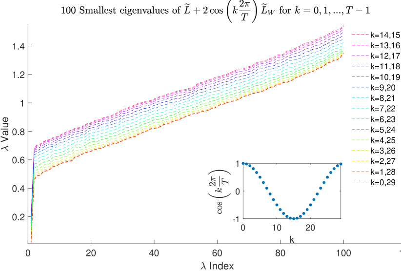
Figure 1: The $100$ smallest eigenvalues of matrices $\tilde{L}+2\cos\left(k\frac{2\pi}{T}\right)\tilde{L}_{W}$ for each $k=0,1,2,...,29$. The matrices $\tilde{L}$ and $\tilde{L}_{W}$ are obtained from a temporal benchmark network composed of $T=30$ Erdos-Renyi random graphs each with $N=100$ nodes and edge probability $p=0.3$ (such dense consecutive ER networks are slowly-changing). The inter-layer weights $\omega$ are fixed at $1$. We include the additional plot of $\cos\left(k\frac{2\pi}{T}\right)$ which determines the monotonically increasing behavior of eigenvalues corresponding to $0\leq k\leq 14$ and monotonically decreasing behaviour of eigenvalues corresponding to $15\leq k\leq 29$.

In Figure 1 we have displayed the first $100$ eigenvalues of the matrix $L=\widetilde{L}+2\cos\left(k\frac{2\pi}{T}\right)\widetilde{L}_{W}$ from equation (7), where we see that for every $j\geq 1,$ the $j^{th}$ eigenvalue $\lambda_{j}^{\left(k\right)}$ of all matrices $\widetilde{L}+2\cos\left(k\frac{2\pi}{T}\right)\widetilde{L}_{W}$ is monotonically increasing with $k$ for

$$0 \leq k\leq\frac{T-1}{2}-1\text{ if }T\text{ is odd}$$

and

$$0 \leq k\leq\frac{T}{2}-1\text{ if }T\text{ is even}.$$

The following proposition explains the behavior of the eigenvalues.

Proposition 3

Without loss of generality assume that $T$ is odd. Then the $j^{th}$ eigenvalues of the matrices $\widetilde{L}+2\cos\left(k\frac{2\pi}{T}\right)\widetilde{L}_{W}$ satisfy

$$\lambda_{j}^{\left(0\right)}\leq\lambda_{j}^{\left(1\right)}\leq\cdot\cdot\cdot\leq\lambda_{j}^{\left(\frac{T-1}{2}-1\right)}.$$

Proof 4

The proof of this proposition is direct consequence of Theorem 8.1.5. in Golub and Van Loan (1996) which states that for symmetric matrices $V$ and $E$ of size $N\times N,$ and for all eigenvalues $\lambda_{j}$, for $j=1,2,...,N,$ hold the inequalities:

$$\lambda_{j}\left(V\right)+\lambda_{\min}\left(E\right)\leq\lambda_{j}\left(V+E\right)\leq\lambda_{j}\left(V\right)+\lambda_{\max}\left(E\right).$$ (9)

We take into account the fact that the eigenvalues of the diagonal matrix $\widetilde{L}_{W}$ are non-negative since they coincide with all non-negative weights $\omega_{j}^{t,p}$. In particular, if all they are equal to a constant $\omega$, then we see that

$$\lambda_{j}^{k}=\lambda_{j}(\widetilde{L})+2\cos\left(k\frac{2\pi}{T}\right)\omega.$$

This completes the proof.

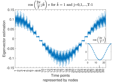
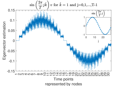
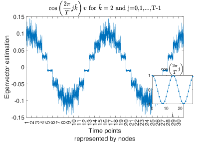
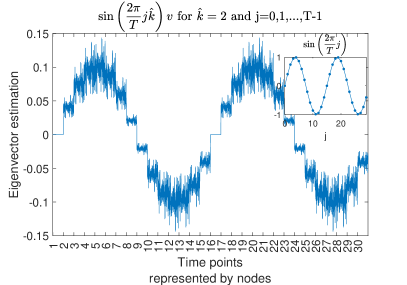
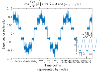
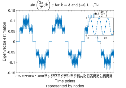
Figure 2: Eigenvector estimations for supra-Laplacian matrix $\mathcal{L}$. This figure visualizes eigenvectors from equation (11) for $\hat{k}=1,2,3,$ each accompanied by the corresponding graph of the $\cos$ and $\sin$ functions. The eigenvector $v$ corresponds to the eigenvalue $\lambda=0$ which is a solution to the eigenvalue problem (7). The matrices $\tilde{L}$ and $\tilde{L}_{W}$ are obtained from a temporal network following the constant block Jacobi model composed of $T=30$ Erdos-Renyi random graphs each with $N=100$ nodes and edge probability $p=0.3$. The inter-layer weights $\omega$ are fixed at $1$.

Figure 3: Eigenvalues and eigenvectors for an Erdos-Renyi benchmark temporal network. The Erdos-Renyi temporal benchmark network is composed of $T=30$ random Erdos-Renyi graphs with $N=100$ nodes and $p=0.1$ edge probability. The inter-layer weights are set to $\omega=0.01$. We plot the $100$ smallest eigenvalues of the corresponding supra-Laplacian matrix, the $6$ eigenvectors corresponding to the $6$ smallest eigenvalues and the $35^{th}$ eigenvector. The jump of the eigenvalue graph indicates precisely the position of $\lambda^{*}$ for index 31 and all following eigenvectors look as the $35^{th}$ eigenvector plotted which captures local variability. Colouring of each eigenvector is consistent with the components that belong to different time points.

Now, by means of Theorem 1, we show how to construct a solution to eigenvalue equation (3) by using equality (7): Fix a $k=\hat{k}$ and consider an eigenvector $v$ with eigenvalue $\hat{\lambda}$ solving the eigenvalue problem (7) for $k=\hat{k}.$ We assume that $\hat{\lambda}$ is among the smallest eigenvalues, close to $0.$ We are seeking for a block-vector $\Psi=\left(\psi_{1},\psi_{2},...,\psi_{T}\right)\in\mathbb{R}^{NT}$ for which $\widehat{\Psi}\left(k\right)=\varphi_{k},$ where the block-vector $\Phi=\left(\varphi_{1},...,\varphi_{T}\right)\in\mathbb{R}^{NT}$ is defined as

$$\varphi_{k}:=\left\{\begin{array}[c]{cc}v&\quad\text{for }k=\hat{k}\\ 0&\quad\text{for }k\neq\hat{k}\end{array}\right.$$

Now we apply the inversion formula (6) to the vector $\Phi,$ and obtain the block-vector $\Psi\in\mathbb{C}^{NT}$ with components

$$\psi_{j}=e^{\frac{2\pi}{T}ij\hat{k}}v\qquad\text{for }j=0,1,...,T-1.$$ (10)

Thus we have $\varphi_{k}=0$ for $k\neq\hat{k},$ and $\Psi$ is a solution to the eigenvalue equation (3) with the same $\hat{\lambda}.$ Since the vector $\Psi$ is complex valued, we obtain two real-valued vectors ($\in\mathbb{R}^{NT}$), by taking the real and imaginary parts of $e^{\frac{2\pi}{T}ij\hat{k}},$ namely:

$$\psi_{j}^{R} :=\cos\left(\frac{2\pi}{T}j\hat{k}\right)\times v\qquad\text{for }j=0,1,...,T-1$$ (11)

$$\psi_{j}^{I} :=\sin\left(\frac{2\pi}{T}j\hat{k}\right)\times v\qquad\text{for }j=0,1,...,T-1$$

In Figure 2 we visualise solutions (11) for $\hat{k}=1,2,3,$ accompanied by the corresponding plots of $\cos(\frac{2\pi}{T}j\hat{k})$ and $\sin(\frac{2\pi}{T}j\hat{k})$ for $j=0,1,...,T-1$.

Every eigenvalue in equation (7) has even multiplicity due to the equality of the two matrices as indicated below:

$$\widetilde{L}+2\cos\left(k\frac{2\pi}{T}\right)\widetilde{L}_{W}= \widetilde{L}+2\cos\left(\left(T-k\right)\frac{2\pi}{T}\right)\widetilde{L}_{W}$$

$$\text{for }0\leq k\leq\frac{T-1}{2}-1;$$

the double multiplicity of the eigenvalues is clearly observed in Figure 1. In the case of odd $T$ there are unique eigenvalues just for $k=\frac{T-1}{2}-1$; for even $T$ all eigenvalues have even multiplicity. For $\hat{k}=0$ we have one solution $\Psi$ with $\psi_{j}=v$ corresponding to the zero eigenvalue, $\hat{\lambda}=0.$

By using the results of perturbation theory for invariant subspaces Golub and Van Loan (1996); Luxburg (2007) we see that for every eigenvalue with even multiplicity, we may estimate the perturbation of its eigenspace, i.e. the space of its eigenvectors. Thus we obtain the solutions which look like “block sinusoids” of $\cos$ and $\sin$ type, Figure 2. The perturbation of the two-dimensional space spanned by $\cos$ and $\sin$ type solutions, results in a two-dimensional space corresponding to the perturbed eigenvalue of the matrix $\mathcal{L}$. These eigenvectors may differ from $\cos$ or $\sin$ type solutions.

The above theoretical results have a direct impact on the eigenvectors of the supra-Laplacian $\mathcal{L}$, Figure 3. We show that the eigenvectors corresponding to the eigenvalues of the supra-Laplacian $\mathcal{L}$, which are close to $0,$ are obtained by perturbation of the eigenvectors corresponding to the $0$ eigenvalues of the separate layers $L^{t}$, derived as $\left(D^{t}\right)^{\frac{1}{2}}\boldsymbol{1}$. Thus they do not carry any information about the finer description of that layer as does the Fiedler vector. These eigenvectors of $\mathcal{L}$ give us only information about all $T$ time layers being separate from each other. The bigger eigenvalues of $\mathcal{L}$ have eigenvectors which are perturbations of mixtures of higher eigenvectors for networks $L^{t}$, i.e. they contain information from the Fiedler eigenvectors for the separate networks $L^{t}$. We can conclude that only after the block nature of the constant block Jacobi model in the temporal network is captured the eigenvectors start capturing variability introduced by some certain within-layer patterns, which is clearly seen from Figure 3.

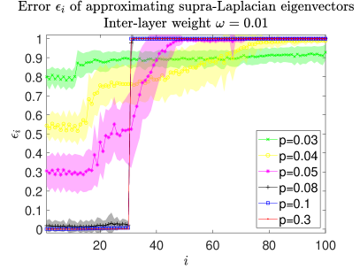
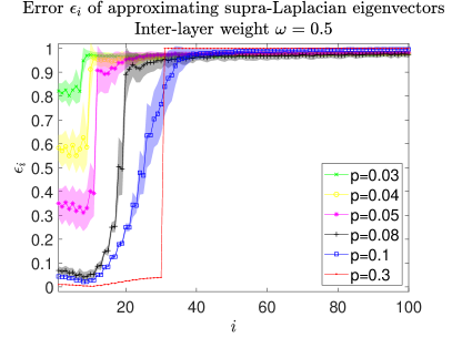
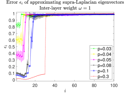
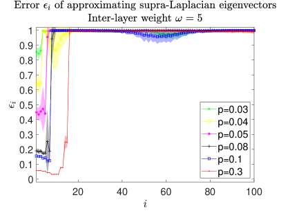
Figure 4: Error $\epsilon_{i}$ of approximating supra-Laplacian eigenvectors (corresponding to eigenvalue $\lambda_{i}$ for $i=1,2,3,....,TN$) by their separate time layers eigenvectors for the benchmark temporal network. All of the benchmark temporal networks were simulated using $T=30$ random Erdos-Renyi graphs with $N=100$ nodes and varying edge probabilities $p=0.03,0.04,0.05,0.08,0.1,0.3$ edge probabilities. Each of the four plots captures the results for different inter-layer weights set to $\omega=0.01,0.05,1,5$. For each parameter combination $(p,\omega)$ we simulate $100$ networks and show their average error $\epsilon_{i}$ with $1$ st.dev. intervals. The obtained approximation average errors and st.dev. intervals are visualized for the first $100$ eigenvectors although at most $T+1$ regressions are needed to capture all $T$ layers as separate layers.

4 Properties of the eigenvectors corresponding to small eigenvalues of the supra-Laplacian $\mathcal{L}$

In this section we empirically showcase the theoretical results that eigenvectors corresponding to the small eigenvalues of $\mathcal{L}$ are well-approximated by linear combinations of the eigenvectors (paired to the zero eigenvalue) of the separate layers. We investigate their behavior with respect to the edge density of the layers and the inter-layer weights.

4.1 Evaluating the approximation of the eigenvectors of $\mathcal{L}$ using the eigenvectors of the separate time layers

Let $\overline{\Lambda}$ be the set of smallest eigenvalues with paired eigenvectors well-approximated by the subspace of eigenvectors corresponding to the $0$ eigenvalues for the separate layers. The theoretical results from Sec. 3 guarantee that the eigenvectors $v$ corresponding to $\lambda\in\overline{\Lambda}$ satisfy (see Sec. 2 for $V^{t}$ def.)

$$\min_{\left\{\alpha_{t}\right\}}\left\|v-\sum_{t=1}^{T}\alpha_{t}V^{t}\right\|\leq\varepsilon$$ (12)

for a small $\varepsilon>0,$ not true for the rest of the eigenvalues.

We evaluate the approximation of each $\mathcal{L}$’s eigenvector $v$ using the eigenvectors of each time layer corresponding to the zero eigenvalue, $V^{t}$, by solving a regression problem where $\varepsilon_{i}$ is the $NT\times 1$ vector of residuals, and we denote the error at $i$ to be $\epsilon_{i}:=\left\|\varepsilon_{i}\right\|$. Denote by $\lambda^{\ast}$ the first eigenvalue $\lambda_{i}$ for which $\epsilon_{i}>>\epsilon_{i-1}$.

4.2 Discussion on the relation between edge density, inter-layer weights and eigenvectors corresponding to the smallest eigenvalues

The present experimental results, in accordance with the developed theory, show that for a small eigenvalue of the supra-Laplacian $\mathcal{L}$, the eigenvectors $\psi^{R}$ and $\psi^{I}$ are approximations to the corresponding eigenvectors of the supra-Laplacian $\mathcal{L}.$ In Figure 3 we observe the eigenvectors of the supra-Laplacian of a temporal network composed of random Erdos-Renyi graphs, Erdos and Renyi (1959). The first few eigenvectors follow the same $\sin$ and $\cos$ functions as seen in Figure 2, and thus can be used to identify the first order approximation by the constant block Jacobi model structure of the temporal network.

We investigate how the approximation of these eigenvectors is affected by the inter-layer weights and the density of the edge weights within each time layer. To showcase this, we simulate various benchmark temporal networks composed of random Erdos-Renyi networks with a varying degree of edge probability ${p=0.03,0.04,0.05,0.08,0.1,0.3}$ and inter-layer weights ${\omega=0.01,0.05,1,5}$, which are two factors that affect the approximation of the eigenvectors of the investigated supra-Laplacians $\mathcal{L}$, Figure 4.

Recall that we have denoted by $\lambda^{\ast}$ the smallest non-zero eigenvalue sensitive to within-layer connectivity patterns, i.e. breaking (12). Then for all benchmark networks types it is true that the value $\lambda^{\ast}$ is increasing with a decreasing $\omega$ value: Smaller inter-layer weights $\omega$ lead to greater separation between time layers, thus more eigenvectors behave as predicted by perturbation theory. More eigenvectors are needed to explain each layer as separate. Higher inter-layer weights influence more the resulting eigenvectors and fewer behave in a way as predicted by perturbation theory. Lower inter-layer weights interfere less and the behaviour of the eigenvectors resembles closely the behaviour of eigenvectors as predicted by perturbation theory.

When the probability $p$ increases, the density within layers $A^{t}$ increases. Since $\omega$ is fixed it cannot reflect on the increasing density of $A^{t}$ and the perturbation effect resulting from inter-layer matrices $W^{t,t+1}$ is smaller. Thus for increasing $p$, i.e. for increasing density, the behaviour of more eigenvectors resembles closely the behaviour of the eigenvectors as predicted by perturbation theory.

When $p$ is decreasing, the eigenvalue $\lambda^{\ast}$ indicates that more eigenvectors resemble closely the behaviour of eigenvectors as predicted by perturbation theory. This is a result of the sparseness of the time layers and the corresponding lower inter-layer weights $\omega_{i}^{t,t+1}$. The above observations need further rigorous theoretical justification.

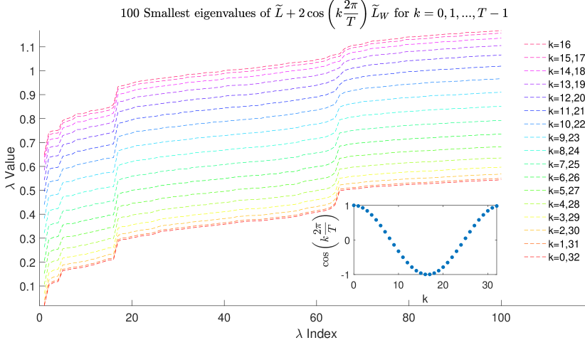
Figure 5: The $100$ smallest eigenvalues of matrices $\tilde{L}+2\cos\left(k\frac{2\pi}{T}\right)\tilde{L}_{W}$ for each $k=0,1,2,...,32$. The matrices $\tilde{L}$ and $\tilde{L}_{W}$ are obtained from a temporal network composed of $T=33$ Sales-Pardo graphs each with $N=640$ nodes. The inter-layer weights $\omega$ are fixed at $1$. We include the additional plot of $\cos\left(k\frac{2\pi}{T}\right)$ which determines the monotonically increasing behaviour for eigenvalues for $0\leq k\leq 15$ and monotonically decreasing behaviour for eigenvalues for $17\leq k\leq 32$.

4.3 Relation between the multi-scale community structure of the layers of a supra-Laplacian network and its eigenvalues.

It is important to note that in Figure 1 the first few eigenvalues capture the block structure of the temporal network following the constant block Jacobi model, thus close to $0$, however after they start monotonically increasing without any clear cuts. From spectral graph partitioning Ding et al. (2001) we know that this is indicative of the lack of structure within the networks, which is the case in here where each layer is a densely connected Erdos-Renyi random graphs with no community structure. In Figure 5, we demonstrate the behavior of the supra-Laplacian eigenvalues when each of the layers has multi-scale community structure simulated using the Sales-Pardo model, Sales-Pardo et al. (2007). Again the smallest eigenvalues capture the block structure of the temporal network, however, there are clear eigenvalue cuts where a new multi-scale community structure within the layers is captured.

5 Conclusions

The above results are crucial in interpreting spectral clustering properties of the supra-Laplacian matrix of all slowly-changing temporal networks that can be represented using a constant block Jacobi model. We have provided experimental results with Erdos-Renyi (unstructured) networks and Sales-Pardo hierarchical networks. Further investigation in these theoretical results will lead into more insights of the spectral properties of supra-Laplacian matrices for more general temporal networks. As presented in the paper, the above findings provide a fundamental understanding of the spectral properties of temporal networks on time periods where they are slowly changing which can significantly improve all spectral-based methods applied on temporal networks such as partitioning, node ranking, community detection, clustering, etc. The above results were successfully used to extend a multiscale community detection method, Tremblay and Borgnat (2014), based on a spectral graph wavelets approach, Hammond et al. (2011), to temporal networks. The extended method, Kuncheva and Montana (2017), takes advantage of the developed theory to automatically detect the different scales at which communities exist across layers, which is an advantage over the multilayer modularity maximization approach, Mucha et al. (2010), used for similar purposes. The above experimental results have been also replicated on temporal Sales-Pardo hierarchical benchmark networks, which are suitable for multi-scale community detection. There is also a detailed investigation of using inter-layer weights that account for the sparsity and similarity across layers, Kuncheva (2017), including a real life application example to social networks data.

6 Acknowledgements

The author OK acknowledges the project KP-06-N52-1 with Bulgarian NSF. The author ZK acknowledges the project KP-06-N32-8 with Bulgarian NSF and EPSRC scholarship (2012-2016) at Imperial College London.

References

- Holme and Saramäki [2012] Petter Holme and Jari Saramäki. Temporal Networks. Phys. Rep., 519(3):97–125, oct 2012. ISSN 03701573. doi:10.1016/j.physrep.2012.03.001.
- Kivelä et al. [2014] Mikko Kivelä, Alexandre Arenas, Marc Barthelemy, James P. Gleeson, Yamir Moreno, and Mason A. Porter. Multilayer Networks. Multilayer Networks, 2(3):203–271, 2014. URL http://arxiv.org/pdf/1309.7233v4.pdf.
- Moreno and Arenas [2013] Y Moreno and A Arenas. Diffusion Dynamics on Multiplex Networks. Phys. Rev. Lett., pages 1–6, 2013.
- Sol et al. [2013] A Sol, M De Domenico, and N E Kouvaris. Spectral Properties of the Laplacian of Multiplex Networks. Phys. Rev. E, 88(3), 2013.
- De Domenico et al. [2016] Manlio De Domenico, Albert Solé-Ribalta, Elisa Omodei, Sergio Gómez, and Alex Arenas. Random Walk Centrality in Interconnected Multilayer Networks. Phys. D Nonlinear Phenom., 323:73–79, nov 2016. URL http://arxiv.org/abs/1311.2906.
- Taylor et al. [2015] Dane Taylor, Sean A. Myers, Aaron Clauset, Mason A. Porter, and Peter J. Mucha. Eigenvector-Based Centrality Measures for Temporal Networks. arxiv Prepr., page 34, jul 2015. URL http://arxiv.org/abs/1507.01266.
- De Domenico et al. [2013] Manlio De Domenico, Albert Solé-Ribalta, Emanuele Cozzo, Mikko Kivelä, Yamir Moreno, Mason A. Porter, Sergio Gómez, and Alex Arenas. Mathematical Formulation of Multilayer Networks. Phys. Rev. X, 3(4):041022, dec 2013. ISSN 2160-3308. doi:10.1103/PhysRevX.3.041022. URL http://link.aps.org/doi/10.1103/PhysRevX.3.041022.
- Chung [1996] Fan Chung. Spectral Graph Theory. CBMS, 1996.
- Luo et al. [2002] Bin Luo, Richard C. Wilson, and Edwin R. Hancock. Spectral Feature Vectors for Graph Clustering. In Terry Caelli, editor, Struct. syntactic, Stat. pattern Recognit., chapter Spectral F, pages 83–93. Springer Berlin Heidelberg, aug 2002. ISBN 3-540-44011-9. URL http://dl.acm.org/citation.cfm?id=645890.758316.
- Luxburg [2007] Ulrike Von Luxburg. A Tutorial on Spectral Clustering. Technical report, Max Planck Institute, 2007. URL http://citeseerx.ist.psu.edu/viewdoc/summary?doi=10.1.1.165.9323.
- Enright and Kao [2018] Jessica Enright and Rowland Raymond Kao. Epidemics on dynamic networks. Epidemics, 24:88 – 97, 2018. ISSN 1755-4365. doi:https://doi.org/10.1016/j.epidem.2018.04.003. URL http://www.sciencedirect.com/science/article/pii/S1755436518300173.
- Bassett et al. [2011] Danielle S Bassett, Nicholas F Wymbs, Mason A Porter, Peter J Mucha, Jean M Carlson, and Scott T Grafton. Dynamic Reconfiguration of Human Brain Networks During Learning. Proc. Natl. Acad. Sci. U. S. A., 108(18):7641–6, may 2011. ISSN 1091-6490. doi:10.1073/pnas.1018985108. URL http://www.pnas.org/cgi/content/long/108/18/7641.
- Mucha et al. [2010] Peter J Mucha, Thomas Richardson, Kevin Macon, Mason A. Porter, and Jukka-Pekka Onnela. Community Structure in Time-Dependent, Multiscale, and Multiplex Networks. Science (80-. )., 328, 2010. URL http://www.sciencemag.org/content/328/5980/876.full.pdf.
- Sahbani [2015] Jaouad Sahbani. Spectral Theory of a Class of Block Jacobi Matrices and Applications. J. Math. Anal. Appl., 438(1):93–118, apr 2015. URL http://arxiv.org/abs/1504.05822.
- Golub and Van Loan [1996] Gene H. Golub and Charles F. Van Loan. Matrix computations. Johns Hopkins University Press, 1996. ISBN 0801854148.
- Erdos and Renyi [1959] Paul Erdos and Alfred Renyi. On Random Graphs, I. Publ. Math., 6:290–297, 1959.
- Ding et al. [2001] Chris Ding, Xiaofeng He, Hongyuan Zha, Ming Gu, and Horst Simon. Spectral min-max cut for graph partitioning and data clustering. Berkley Lab, 2001.
- Sales-Pardo et al. [2007] Marta Sales-Pardo, Roger Guimerà, André A Moreira, and Luís A Nunes Amaral. Extracting the Hierarchical Organization of Complex Systems. Proc. Natl. Acad. Sci. U. S. A., 104(39):15224–9, sep 2007. ISSN 0027-8424. doi:10.1073/pnas.0703740104. URL http://www.pnas.org/content/104/39/15224.abstract.
- Tremblay and Borgnat [2014] Nicolas Tremblay and Pierre Borgnat. Graph Wavelets for Multiscale Community Mining. IEEE Trans. Signal Process., 62(20):5227–5239, oct 2014. ISSN 1053-587X. doi:10.1109/TSP.2014.2345355. URL http://ieeexplore.ieee.org/lpdocs/epic03/wrapper.htm?arnumber=6870496.
- Hammond et al. [2011] David K. Hammond, Pierre Vandergheynst, and Rémi Gribonval. Wavelets on Graphs via Spectral Graph Theory. Appl. Comput. Harmon. Anal., 30(2):129–150, mar 2011. ISSN 10635203. doi:10.1016/j.acha.2010.04.005. URL http://www.sciencedirect.com/science/article/pii/S1063520310000552.
- Kuncheva and Montana [2017] Zhana Kuncheva and Giovanni Montana. Multi-scale community detection in temporal networks using spectral graph wavelets. International Workshop on Personal Analytics and Privacy, 10708:139–154, 2017.
- Kuncheva [2017] Zhana Kuncheva. Modelling Populations of Complex Networks. PhD thesis, Department of Mathematics, Imperial College London, 2017.