Nonthermal radiation of evaporating black holes

Abstract

Black hole (BH) evaporation is caused by creation of entangled particle-antiparticle pairs near the event horizon, with one carrying positive energy to infinity and the other carrying negative energy into the BH. Since under the event horizon, particles always move toward the BH center, they can only be absorbed but not emitted at the center. This breaks absorption-emission symmetry and, as a result, annihilation of the particle at the BH center is described by a non-Hermitian Hamiltonian. We show that due to entanglement between photons moving inside and outside the event horizon, non-unitary absorption of the negative energy photons near the BH center, alters the outgoing radiation. As a result, radiation of the evaporating BH is not thermal, it carries information about BH interior and entropy is preserved during evaporation.

I Introduction

According to principles of quantum mechanics, state of an isolated system remains pure during evolution. This is the case for both types of quantum mechanical evolution - a unitary evolution governed by the Schrödinger equation and a non-unitary state vector collapse brought about by a measurement. If the system remains in a pure state the von Neumann entropy is preserved.

Computations of Hawking radiation, which is believed to be produced by an evaporating black hole (BH), indicated that it is completely thermal [1, 2, 3, 4]. Therefore, an evaporating BH would eventually leave behind a cloud of thermal radiation, independently of the initial state from which it was formed. However, one could imagine forming a BH from a pure state that seems to evolve to a mixed thermal state which amounts to a loss of information and thus is incompatible with quantum mechanical evolution. This is known as the BH information paradox [5]. For proposals to resolve the BH information problem see, e.g., [6, 7] and references therein.

According to the holographic principle, the bulk information in models of gravity in $d$-dimensions might be available on the $d-1$ dimensional boundary of spacetime [8, 9]. Holography of information implies that the internal quantum state of a BH must be encoded in the asymptotic quantum state of its graviton field, since otherwise the information would not be recoverable at the boundary [10, 11]. In [12, 13] it has been shown explicitly that information about the BH internal state is available in the quantum state of its gravity field (quantum hair). Moreover, it has been argued that long wavelength gravitons can give rise to an infinite number of conserved charges which preserve an infinite amount of information outside BHs [14] which could give a new perspective on the information problem [15, 16].

Holography was given an explicit realization in the AdS/CFT correspondence of Maldacena [17], which suggests that BH evaporation can be unitary. Recently there has been considerable progress in directly computing the entanglement entropy of evaporation using AdS methods, and these results suggest that the process is unitary [18]. While both holography of information and AdS/CFT duality suggest that the BH information paradox is somehow resolved in favor of unitarity, neither yield a specific description of the physical process by which BH information is encoded in Hawking radiation.

Here we show that entanglement of particle pairs generated during BH evaporation, combined with non-unitary absorption of particles near the BH center, leads to nonthermal outgoing radiation that carries information about the BH interior.

BHs possess an event horizon - the boundary under which no particles, at least if they are treated classically and moving forward in time, can escape. This leads to a believe that an observer outside the BH has no access to the interior part of the total quantum system, and information about the internal degrees of freedom is lost during BH evaporation leaving the system in a mixed state.

However, BH spacetime has another inherent feature, namely, under the event horizon, particles always move toward the BH center. The latter probably has a Planck scale and is described by yet not well-understood physics. What matters for the present discussion is that, since particles can move only towards the center, photons with a wavelength much greater than the Plank length can only be absorbed, but not emitted at the BH center.

Emitted particles move away from the source and, since particles cannot move away from the BH center, they cannot be emitted in this region. This breaks the symmetry between absorption and emission. As a result, annihilation of the particle at the BH center is described by a non-Hermitian Hamiltonian.

Here we show that if the emission-absorption symmetry is broken, quantum mechanics predicts that radiation of an evaporating BH is nonthermal and it carries information about the state of matter in the BH interior. Next we briefly discuss the physics of Hawking radiation from a negative frequency perspective [19].

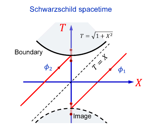
Figure 1: Schwarzschild spacetime in the Kruskal-Szekeres coordinates. A space-like line $T=\sqrt{1+X^{2}}$ sets the spacetime boundary. Unruh vacuum is filled with entangled right-moving Rindler photons $\phi_{1}$ and $\phi_{2}$ which are localized outside and inside the BH event horizon (line $T=X$) respectively. Absorption of Rindler photons $\phi_{2}$ at the boundary reduces BH mass and leads to BH evaporation. We model the boundary as a set of harmonic oscillators that absorb all ingoing photons, but do not emit. Due to vacuum entanglement, the process looks like as if there is a mirror “image” of the oscillators located along the line $T=-\sqrt{1+X^{2}}$ which emit (but do not absorb) light outside the BH event horizon.

II Hawking radiation from a negative frequency perspective

According to general relativity, a static BH of mass $M$ in 3+1 dimension in Schwarzschild coordinates is described by a metric

$$ds^{2}=\left(1-\frac{r_{g}}{r}\right)c^{2}dt^{2}-\frac{1}{1-\frac{r_{g}}{r}}dr^{2}-r^{2}\left(d\theta^{2}+\sin^{2}\theta d\varphi^{2}\right),$$ (1)

where $r_{g}=2GM/c^{2}$ is the gravitational radius. For simplicity, we truncate the spacetime to 1+1 dimension ($t$ and $r$, where $r\geq 0$) and use Kruskal-Szekeres coordinates $T$ and $X$ that are defined in terms of the Schwarzschild coordinates $t$ and $r$ as

$$T=\sqrt{r/r_{g}-1}e^{\frac{r}{2r_{g}}}\sinh\left(\frac{ct}{2r_{g}}\right),$$ (2)

$$X=\sqrt{r/r_{g}-1}e^{\frac{r}{2r_{g}}}\cosh\left(\frac{ct}{2r_{g}}\right),$$ (3)

for $r>r_{g}$, and

$$T=\sqrt{1-r/r_{g}}e^{\frac{r}{2r_{g}}}\cosh\left(\frac{ct}{2r_{g}}\right),$$ (4)

$$X=\sqrt{1-r/r_{g}}e^{\frac{r}{2r_{g}}}\sinh\left(\frac{ct}{2r_{g}}\right),$$ (5)

for $0<r<r_{g}$. In these coordinates, the BH center ($r=0$) is a space-like line $T=\sqrt{1+X^{2}}$. This line sets a boundary of the Schwarzschild spacetime in the Kruskal-Szekeres coordinates (see Fig. 1). The boundary appears because coordinate transformation (2)-(5) maps the region $-\infty<t<\infty$, $r\geq 0$ into $T\leq\sqrt{1+X^{2}}$, $T\geq-X$. In the Kruskal-Szekeres coordinates, in 1+1 dimension, the Schwarzschild metric

$$ds^{2}=\frac{4r_{g}^{3}}{r}e^{-r/r_{g}}\left(dT^{2}-dX^{2}\right)$$ (6)

is conformally invariant to the Minkowski metric and, thus, a massless scalar field $\phi$ obeys the same wave equation as in the Minkowski spacetime

$$\left(\frac{\partial^{2}}{\partial T^{2}}-\frac{\partial^{2}}{\partial X^{2}}\right)\phi=0.$$ (7)

For the present problem only the right-moving field in Fig. 1 is important. It is convenient to describe such a field using Rindler modes [20]

$$\phi_{1\Omega}(T,X)=(X-T)^{i\Omega}\theta(X-T),$$ (8)

$$\phi_{2\Omega}(T,X)=(T-X)^{-i\Omega}\theta(T-X),$$ (9)

where $\Omega>0$ is a parameter, and $\theta$ is the Heaviside step function. Rindler modes $\phi_{1\Omega}$ and $\phi_{2\Omega}$ are solutions of the wave equation (7), and for $\Omega>0$ have positive norm (defined as the Klein–Gordon inner product). The mode functions (8) and (9) are non-zero outside and inside the BH event horizon (line $T=X$) respectively (see Fig. 1). These two regions are causally disconnected for the right-moving field. Annihilation operators of the Rindler photons we denote as $\hat{b}_{1\Omega}$ and $\hat{b}_{2\Omega}$.

It is believed that, to a good approximation, Unruh vacuum $|0_{U}\rangle$ describes state of the field produced by a gravitational collapse of a star into a BH. In this state, there are no left-moving Rindler photons and no right-moving Minkowski photons [3]. That is, Unruh vacuum is Rindler vacuum for the left-moving photons and Minkowski vacuum for the right-moving photons. In terms of the right-moving Rindler photons, which are relevant for the present discussion, the Unruh vacuum is a squeezed state [21]

$$\left|0_{U}\right\rangle=\prod\limits_{\Omega>0}\sqrt{1-\gamma^{2}}e^{\gamma\hat{b}_{1\Omega}^{\dagger}\hat{b}_{2\Omega}^{\dagger}}\left|0_{R}\right\rangle,$$ (10)

where

$$\gamma=e^{-\pi\Omega},$$ (11)

$\left|0_{R}\right\rangle$ refers to the Rindler vacuum, $\hat{b}_{1\Omega}^{\dagger}$ and $\hat{b}_{2\Omega}^{\dagger}$ are creation operators of the right-moving Rindler photons. That is, Unruh vacuum is filled with the right-moving Rindler photons, but it looks empty if the right-moving field is described by means of the Minkowski photons.

If a hypothetical observer is located at the BH center ($r=0$), then Schwarzschild coordinate $t$ is the proper time for such observer. Recall that proper time of an object is the coordinate which changes in the object’s frame. If the object is held fixed at $r=const$ then $t$ is the proper time. In the region $0<r<r_{g}$, it is physically impossible to hold particles fixed at $r=const$, that’s why we use the word “hypothetical”. Eqs. (4), (5) and (9) yield that at the BH center the non-zero Rindler mode $\phi_{2\Omega}$ oscillates as a function of $t$ as $\phi_{2\Omega}\propto e^{i\Omega ct/2r_{g}}$. That is, from the observer’s perspective the Rindler photons behave as if they have negative frequency $-\Omega c/2r_{g}$ [19]. Hence, in the Unruh vacuum, there is a flux of the negative frequency (energy) Rindler photons into the BH center. Absorption of such photons near the BH center decreases energy (mass) of the BH, leading to BH evaporation.

If an observer is held fixed outside the event horizon at a constant Schwarzschild coordinate $r$, then at the observer’s location the non-zero Rindler modes $\phi_{1\Omega}$ oscillate as $\phi_{1\Omega}\propto e^{-i\Omega ct/2r_{g}}$, where $t$ is the observer’s proper time. That is, from the external observer perspective the Rindler photons behave as if they have positive frequency

$$\nu=\frac{\Omega c}{2r_{g}}$$ (12)

and, thus, they can excite a detector. Photons $\phi_{1\Omega}$ propagate away from the BH.

For simplicity, we will assume that the field has only modes with one “frequency” $\Omega$. We denote such Rindler modes as $\phi_{1}$ and $\phi_{2}$. Then Unruh vacuum can be written as

$$\left|0_{U}\right\rangle=\sqrt{1-\gamma^{2}}e^{\gamma\hat{b}_{1}^{\dagger}\hat{b}_{2}^{\dagger}}\left|0_{R}\right\rangle=\sqrt{1-\gamma^{2}}\sum_{n=0}^{\infty}\gamma^{n}\left|nn\right\rangle,$$ (13)

where $\left|nn\right\rangle$ is a state with $n$ Rindler photons in the modes $\phi_{1}$ and $\phi_{2}$.

If modes $\phi_{1}$ and $\phi_{2}$ are considered separately, then tracing over or absorbing one of the modes leaves the remaining mode in a thermal state. Namely, if we trace over the Rindler modes under the event horizon $\phi_{2}$, which are not accessible to the external observer, the reduced density operator for the field $\phi_{1}$ is thermal

$$\hat{\rho}_{1}=\text{Tr}_{2}\left(\left|0_{U}\right\rangle\left\langle 0_{U}\right|\right)=\left(1-\gamma^{2}\right)\sum_{n=0}^{\infty}\gamma^{2n}\left|n\right\rangle\left\langle n\right|$$ (14)

with the average number of photons

$$\bar{n}_{1}=\frac{\gamma^{2}}{1-\gamma^{2}}.$$ (15)

Thus, an observer held fixed outside the BH horizon feels thermal radiation coming out from the BH, which is known as Hawking radiation. Using Eqs. (11), (12) and (15), one can write $\bar{n}_{1}$ as a Planck factor

$$\bar{n}_{1}=\frac{1}{e^{\frac{4\pi r_{g}\nu}{c}}-1}=\frac{1}{e^{\frac{\hbar\nu}{k_{B}T_{H}}}-1}$$ (16)

with the Hawking temperature $T_{H}=\hbar c/4\pi k_{B}r_{g}$.

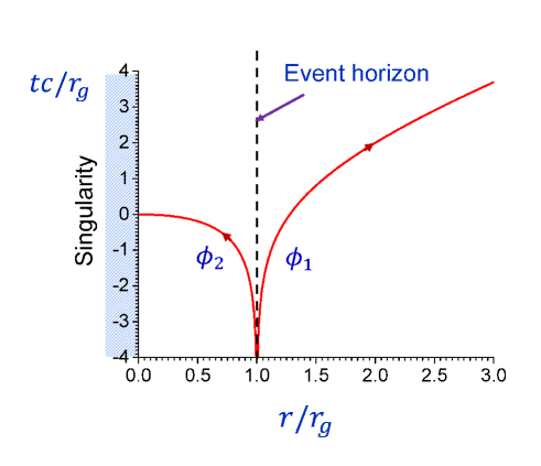
Figure 2: Light rays of Rindler photons $\phi_{1}$ and $\phi_{2}$ in Schwarzschild coordinates.

Figure 2 shows light rays of Rindler photons (8) and (9) in the Schwarzschild coordinates. It looks like the negative ($\phi_{2}$) and positive ($\phi_{1}$) frequency Rindler photons are generated at the event horizon. This is consistent with the interpretation of the Hawking radiation as a continuous creation of particle-antiparticle pairs near the event horizon, with one carrying positive energy to infinity and the other carrying negative energy into the BH [22]. Calculations of the energy-momentum tensor for the field near an evaporating BH directly show that there is a negative-energy flux into the BH center and a positive-energy flux far away from the BH [23].

III Model of an evaporating black hole taking into account non-unitary photon absorption at the center

According to Eq. (7), in the Kruskal-Szekeres coordinates the field evolves following the same wave equation as in Minkowski spacetime. For the latter, absorption or emission of photons in the region $T>X$ cannot affect the state of the field in the region $T<X$. However, the BH spacetime has a space-like boundary at $T=\sqrt{1+X^{2}}$. We will show below that absorption of photons at the boundary changes the state of the field outside the event horizon and radiation of the evaporating BH is not thermal. We will assume that Unruh vacuum is the state of the field only at the onset of evaporation and calculate how the field evolves.

According to general relativity, spacetime disappears at the BH center (spacetime boundary). It is assumed that matter disappears together with the spacetime, but state of matter (mass, angular momentum, etc.) is recorded in the gravitational field near the BH center. This process transfers characteristics of the accreting matter into the BH internal gravitational field.

The worldlines of the Rindler photons $\hat{b}_{2}$ terminate at the spacetime boundary (see Fig. 1). But we can’t just say that photons disappear. One should describe this process quantum mechanically using a Hamiltonian. Space-like boundary breaks the symmetry between emission and absorption of Rindler photons $\hat{b}_{2}$. Namely, if backward in time propagation is not allowed, Rindler photons $\hat{b}_{2}$ cannot be emitted at the boundary because such a process means emission of particles outside the spacetime.

Next we consider a simple toy model of BH evaporation modeling the boundary as a set of harmonic oscillators that totally absorb the ingoing field. The oscillators follow the worldline of the boundary which is not geodesic. We do not associate the oscillators with ordinary particles. Rather, the oscillators provide a physical model of the gravitational field near the BH center that carries information about the state of the BH interior. In our model, the oscillator’s energy is the origin of the BH mass. As we showed above, from the oscillator’s perspective, Rindler photons have negative energy. Thus, absorption of Rindler photons reduces the energy of the oscillators (BH mass decreases).

Since oscillators are under the BH horizon, they can interact only with photons $\hat{b}_{2}$. In the toy model, the interaction Hamiltonian describing BH evaporation reads

$$\hat{V}_{2}(t)=g\hat{\sigma}e^{-i\omega t}\phi_{2}(t)\hat{b}_{2},$$ (17)

where $\hat{\sigma}$ is the lowering operator for the oscillator of frequency $\omega$, $g$ is the coupling constant and the field mode function $\phi_{2}(T,X)$ is taken at the location of the oscillator $\phi_{2}(t)=\phi_{2}(T(t,0),X(t,0))=e^{i\frac{c\Omega t}{2r_{g}}}$. In Eq. (17), $t$ is the proper time of the oscillator which coincides with the Schwarzschild coordinate $t$ because oscillators are located at fix $r=0$. Since oscillators cannot emit Rindler photons, the Hamiltonian (17) is not Hermitian.

We will consider evolution of the system as a function of the oscillator proper time $t$. Schrödinger equation for the system’s state vector

$$i\hslash\frac{\partial}{\partial t}\left|\psi(t)\right\rangle=\hat{V}_{2}(t)\left|\psi(t)\right\rangle$$

yields

$$\left|\psi(t)\right\rangle=e^{\beta(t)\hat{\sigma}\hat{b}_{2}}\left|0_{U}\right\rangle\left|A\right\rangle,$$ (18)

where $\left|0_{U}\right\rangle$ and $\left|A\right\rangle$ are the initial state vectors of the field and the oscillator, and

$$\beta(t)=-\frac{ig}{\hslash}\int_{0}^{t}dt^{\prime}e^{-i\omega t^{\prime}}\phi_{2}(t^{\prime})=-\frac{ig}{\hslash}\int_{0}^{t}dt^{\prime}e^{i\left(\frac{c\Omega}{2r_{g}}-\omega\right)t^{\prime}}.$$

Plug $\left|0_{U}\right\rangle$ in Eq. (18) gives

$$\left|\psi(t)\right\rangle=\sqrt{1-\gamma^{2}}e^{\beta(t)\hat{\sigma}\hat{b}_{2}}e^{\gamma\hat{b}_{1}^{\dagger}\hat{b}_{2}^{\dagger}}\left|0_{R}\right\rangle\left|A\right\rangle.$$ (19)

Using the Baker–Hausdorff formula $e^{\hat{A}}e^{\hat{B}}=e^{[\hat{A},\hat{B}]}e^{\hat{B}}e^{\hat{A}}$, we obtain

$$\left|\psi(t)\right\rangle=\sqrt{1-\gamma^{2}}e^{\gamma\beta(t)\hat{\sigma}\hat{b}_{1}^{\dagger}}e^{\gamma\hat{b}_{1}^{\dagger}\hat{b}_{2}^{\dagger}}e^{\beta(t)\hat{\sigma}\hat{b}_{2}}\left|0_{R}\right\rangle\left|A\right\rangle,$$

or

$$\left|\psi(t)\right\rangle=e^{\gamma\beta(t)\hat{\sigma}\hat{b}_{1}^{\dagger}}\left|0_{U}\right\rangle\left|A\right\rangle.$$ (20)

Equation (20) shows that non-unitary field absorption at the spacetime boundary yields generation of photons outside the BH event horizon (into the Rindler mode $1$). Taking time derivative of Eq. (20) leads to the Schrödinger equation with the interaction Hamiltonian

$$\hat{V}_{1}(t)=\gamma g\hat{\sigma}e^{-i\omega t}\phi_{1}^{\ast}(t)\hat{b}_{1}^{\dagger},$$

where we used $\phi_{2}(t)=\phi_{1}^{\ast}(t)=\phi_{1}^{\ast}(-T(t,0),X(t,0))$.

That is, the process looks like as if there is a mirror “image” of the oscillator located along the line $T=-\sqrt{1+X^{2}}$ (see Fig. 1) which is coupled with the external mode $\phi_{1}$ with a reduced coupling constant $\gamma g$. The oscillator’s image produces field outside the event horizon which propagates away from the BH. Such field is not thermal. E.g., if the oscillator is in a coherent state, the generated field is coherent. The information stored in the oscillators is recorded in the outgoing field.

BH radiation is not thermal because evolution of the field under the horizon is described by the non-Hermitian Hamiltonian (17). Indeed, if the Hamiltonian would be Hermitian and depends only on $\hat{b}_{2}$ and $\hat{b}_{2}^{\dagger}$, the Heisenberg equation of motion for the operator $\hat{b}_{1}(t)$

$$\frac{d\hat{b}_{1}(t)}{dt}=\frac{i}{\hslash}\left(\hat{H}^{\dagger}\hat{b}_{1}(t)-\hat{b}_{1}(t)\hat{H}\right)=\frac{i}{\hslash}\left(\hat{H}^{\dagger}(t)-\hat{H}(t)\right)\hat{b}_{1}$$ (21)

would yield $\hat{b}_{1}(t)=const$. That is field outside the BH event horizon would not change. However, if $\hat{H}^{\dagger}\neq\hat{H}$, the right-hand-side of Eq. (21) is no longer zero and the external field can be altered.

In the present model of BH evaporation the von Neumann entropy is preserved. Namely, since evolution of the system is described by a Hamiltonian, the system remains in a pure state and, thus, the net entropy remains equal to zero. This is true even if the Hamiltonian is not Hermitian. For the latter, the system’s state vector should be normalized such that $\left\langle\psi\right.\left|\psi\right\rangle=1$.

The toy model Hamiltonian (17) explains why non-unitary absorption of photons at the BH center alters radiation outside the BH. However, it does not describe the system’s dynamics correctly. The point is that, non-Hermitian Hamiltonians don’t preserve the expectation value of an operator $\hat{Q}$ with which they commute. This is the reason why the norm of the state vector is not conserved (in this case $\hat{Q}=1$). To incorporate a conservation law $\left\langle\hat{Q}\right\rangle=const$ into the model, we must replace the non-Hermitian Hamiltonian $\hat{H}$ with a constrained Hamiltonian [24, 25]

$$\hat{H}-\lambda(t)\hat{Q},$$ (22)

where $\lambda(t)$ is a Lagrange multiplier whose value is to be chosen so as to honor the constraint condition $\left\langle\hat{Q}\right\rangle=const$.

We will impose a constraint that during BH evaporation the average energy is conserved. Operators describing conserved quantities must commute with the Hamiltonian. Such “energy” operators commuting with the Hamiltonian (17) are

$$\hat{\sigma}^{\dagger}\hat{\sigma}-\hat{b}_{2}^{\dagger}\hat{b}_{2},\text{\ and }\hat{b}_{1}^{\dagger}\hat{b}_{1},$$

and the constraints read

$$\left\langle\hat{\sigma}^{\dagger}\hat{\sigma}-\hat{b}_{2}^{\dagger}\hat{b}_{2}\right\rangle=const\text{ \ and \ }\left\langle\hat{b}_{1}^{\dagger}\hat{b}_{1}\right\rangle=const.$$ (23)

The constrained interaction Hamiltonian is

$$\hat{V}(t)=g\hat{\sigma}e^{-i\omega t}\phi_{2}(t)\hat{b}_{2}+i\hslash\hat{C}(t),$$ (24)

where

$$\hat{C}(t)=\dot{\mu}_{1}(t)\hat{b}_{1}^{\dagger}\hat{b}_{1}+\dot{\mu}_{2}(t)\left(\hat{\sigma}^{\dagger}\hat{\sigma}-\hat{b}_{2}^{\dagger}\hat{b}_{2}\right)+\dot{\mu}_{3}(t)$$

and the dot denotes derivative over $t$. The latter is introduced for convenience. We assume that the resonance condition $\omega=c\Omega/2r_{g}$ is satisfied, which yields

$$\hat{V}(t)=g\hat{\sigma}\hat{b}_{2}+i\hslash\hat{C}(t).$$ (25)

The Lagrange multiplier $\dot{\mu}_{3}(t)$ takes into account the normalization condition $\left\langle\psi\right.\left|\psi\right\rangle=1$. For the present problem, Lagrange multipliers $\dot{\mu}_{1,2,3}(t)$ are real functions.

We assume that initially the oscillator is in a coherent state $\left|A\right\rangle$ and the field is in the Unruh vacuum $\left|0_{U}\right\rangle$. Schrödinger equation with the constrained Hamiltonian (25) yields (see Appendix A and B)

$$\left|\psi(t)\right\rangle=N(t)e^{-\frac{i}{\hslash}\gamma gAe^{\mu_{1}(t)}t\hat{b}_{1}^{\dagger}}e^{e^{\mu_{1}(t)-\mu_{2}(t)}\gamma\hat{b}_{1}^{\dagger}\hat{b}_{2}^{\dagger}}\left|0_{R}\right\rangle\left|e^{\mu_{2}(t)}A\right\rangle,$$ (26)

where $N(t)$ is a normalization factor and the Lagrange multipliers are obtained from the constraint equations

$$e^{2\mu_{2}}A^{2}-\frac{\tilde{\gamma}^{2}}{1-\tilde{\gamma}^{2}}-\frac{e^{2\mu_{1}}\tilde{\gamma}^{2}\left(\gamma\Lambda t\right)^{2}}{\left(1-\tilde{\gamma}^{2}\right)^{2}}=A^{2}-\frac{\gamma^{2}}{1-\gamma^{2}},$$ (27)

$$\frac{\tilde{\gamma}^{2}}{1-\tilde{\gamma}^{2}}+\frac{e^{2\mu_{1}}\left(\gamma\Lambda t\right)^{2}}{\left(1-\tilde{\gamma}^{2}\right)^{2}}=\frac{\gamma^{2}}{1-\gamma^{2}},$$ (28)

where $\tilde{\gamma}=e^{\mu_{1}-\mu_{2}}\gamma$ and $\Lambda=gA/\hslash$ is the Rabi frequency. For $t\rightarrow\infty$, Eqs. (26)-(28) give

$$\left|\psi(\infty)\right\rangle=Ne^{-\frac{i\gamma}{\sqrt{1-\gamma^{2}}}\hat{b}_{1}^{\dagger}}\left|0_{R}\right\rangle\left|A_{\infty}\right\rangle,$$ (29)

where

$$A_{\infty}^{2}=A^{2}-\frac{\gamma^{2}}{1-\gamma^{2}}$$ (30)

is the mean number of oscillator excitations in the final state. The present model of the spacetime boundary is self-consistent if the oscillators absorb all ingoing photons, which implies $A_{\infty}^{2}>0$. Otherwise, photon flux through the boundary would be nonzero.

Eq. (29) shows that the final state of the field is the Rindler vacuum for photons $\hat{b}_{2}$ and a coherent state for photons $\hat{b}_{1}$ with the average photon number $\gamma^{2}/(1-\gamma^{2})$. The oscillator remains in the coherent state, but the oscillator’s mean excitation number is reduced by an amount $\gamma^{2}/(1-\gamma^{2})$ due to absorption of all $\hat{b}_{2}$ photons.

For in our model $\left\langle\hat{b}_{1}^{\dagger}\hat{b}_{1}\right\rangle=const$, the radiation power of an evaporating BH is given by the Hawking’s formula, but photon statistics is not thermal and the outgoing radiation carries information about the BH interior. In particular, coherent oscillations of the BH interior lead to a coherent outgoing radiation.

In the limit $\gamma\ll 1$, Eqs. (27) and (28) can be solved analytically yielding the following expression for the system’s state vector as a function of $t$

$$\left|\psi(t)\right\rangle=N(t)e^{-\frac{i\gamma\Lambda t\hat{b}_{1}^{\dagger}}{\sqrt{1+\Lambda^{2}t^{2}}}}e^{\frac{\gamma\hat{b}_{1}^{\dagger}\hat{b}_{2}^{\dagger}}{\sqrt{1+\Lambda^{2}t^{2}}}}\left|0_{R}\right\rangle\left|A(t)\right\rangle,$$ (31)

where

$$A^{2}(t)=A^{2}-\frac{\Lambda^{2}t^{2}}{1+\Lambda^{2}t^{2}}\gamma^{2}.$$

According to Eq. (31), initial thermal Hawking radiation evolves into the coherent state $e^{-i\gamma\hat{b}_{1}^{\dagger}}\left|0_{R}\right\rangle$ on a time scale $1/\Lambda$, while the oscillator’s energy (BH mass) decreases as $\hslash\omega A^{2}(t)$.

IV Insights from quantum gravity models

Here we show that present mechanism of nonthermal emission of evaporating BHs holds for an effective metric obtained in quantum gravity models. Most of such models suggest that the classical singularity at $r=0$ should be replaced by a regular timelike boundary. To be specific, we consider an effective BH metric obtained from scale-dependent effective average action which takes into account the effect of all loops [26, 27, 28]. As a function of this scale, the effective average action satisfies a renormalization group equation yielding the effective metric [29]

$$ds^{2}=f(r)c^{2}dt^{2}-\frac{1}{f(r)}dr^{2}-r^{2}\left(d\theta^{2}+\sin^{2}\theta d\varphi^{2}\right),$$ (32)

where

$$f(r)=1-\frac{r_{g}}{r}\frac{1}{1+\frac{\bar{\omega}r_{g}^{2}}{r^{2}}},$$ (33)

and $\bar{\omega}>0$ is a constant that involves the quantum gravity correction to the BH geometry coming from the renormalization group approach.

The metric (32) is regular at $r=0$ and has two horizons which can be found by setting $f(r)=0$ in Eq. (33). The position of the outer and inner horizons is

$$r_{\pm}=\frac{r_{g}}{2}\left(1\pm\sqrt{1-4\bar{\omega}}\right).$$

In terms of $r_{\pm}$, one can write

$$\frac{1}{f(r)}=1+\frac{r_{g}r}{(r-r_{-})(r-r_{+})}.$$

A massless scalar field $\phi$ obeys the covariant wave equation

$$\frac{1}{\sqrt{-g}}\frac{\partial}{\partial x^{\mu}}\left(\sqrt{-g}g^{\mu\nu}\frac{\partial\phi}{\partial x^{\nu}}\right)=0,$$ (34)

where $g^{\mu\nu}$ is the spacetime metric given by the interval (32), namely

$$g^{tt}=\frac{1}{f(r)},\quad g^{rr}=-f(r).$$

For the truncated 1+1 dimensional spacetime $\sqrt{-g}=1$, and the wave equation (34) reduces to

$$\frac{1}{c^{2}}\frac{\partial^{2}\phi}{\partial t^{2}}-f(r)\frac{\partial}{\partial r}\left(f(r)\frac{\partial\phi}{\partial r}\right)=0.$$ (35)

Solutions of Eq. (35) read

$$\phi_{\nu}(t,r)=e^{-i\nu\left[t\pm\frac{r}{c}\mp\chi(r)\right]},$$ (36)

where

$$\chi(r)=\frac{r_{-}\ln|r-r_{-}|-r_{+}\ln|r-r_{+}|}{c\sqrt{1-4\bar{\omega}}}.$$

Using Eq. (36), one can construct mode functions analogous to the Rindler modes (8) and (9) in the Schwarzschild coordinates, namely,

$$\phi_{1\nu}(t,r)=e^{-i\nu\left[t-\frac{r}{c}+\chi(r)\right]}\theta(r-r_{+}),$$ (37)

$$\phi_{2\nu}(t,r)=e^{i\nu\left[t-\frac{r}{c}+\chi(r)\right]}\theta(r_{+}-r)\theta(r-r_{-}),$$ (38)

where $\nu>0$. For $r_{-}=0$, the mode functions (37) and (38) reduce to Eqs. (8) and (9) with $\Omega=2r_{g}\nu/c$.

Eqs. (37) and (38) show that if an observer is held fixed outside the outer event horizon at a constant $r>r_{+}$, then at the observer’s location the non-zero Rindler modes $\phi_{1\nu}$ oscillate as $\phi_{1\nu}\propto e^{-i\nu t}$, where $t$ is the observer’s proper time. That is, from the observer’s perspective, the Rindler photons $\phi_{1\nu}$ behave as if they have positive frequency $\nu$. However, if a hypothetical observer is located at fixed $r_{-}<r<r_{+}$, the non-zero Rindler mode $\phi_{2\nu}$ oscillates as a function of the proper time $t$ as $\phi_{2\nu}\propto e^{i\nu t}$. That is, from the observer’s perspective, the Rindler photons $\phi_{2\nu}$ behave as if they have negative frequency $-\nu$. Absorption of photons $\phi_{2\nu}$ decreases energy (mass) of the BH, leading to BH evaporation.

Photons falling into the BH from BH exterior are described by the mode functions

$$\phi_{3\nu}(t,r)=e^{-i\nu\left[t+\frac{r}{c}-\chi(r)\right]}-e^{i\varphi_{0}}e^{-i\nu\left[t-\frac{r}{c}+\chi(r)\right]}\theta(r_{-}-r),$$ (39)

where the last term describes a wave reflected from the timelike spacetime boundary $r=0$, and $\varphi_{0}$ is a phase shift introduced to satisfy the reflective boundary condition, e.g., $\left.\partial\phi_{3\nu}/\partial r\right|_{r=0}=0$. From the perspective of an observer held fixed at $r=const$ the mode functions $\phi_{3\nu}$ have positive frequency. Thus, absorption of such photons increases the BH mass.

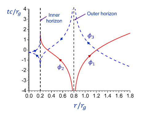
Figure 3: Light rays of photons $\phi_{1\nu}$, $\phi_{2\nu}$ (solid line) and $\phi_{3\nu}$ (dash line) in the metric (32) for $r_{-}=0.2r_{g}$ and $r_{+}=0.8r_{g}$.

In Fig. 3 we plot light rays of photons (37), (38) and (39) in the Schwarzschild coordinates. The figure shows that the negative ($\phi_{2\nu}$) and positive ($\phi_{1\nu}$) frequency Rindler photons are generated at the outer horizon. These photons are produced in pairs and are entangled. Photons $\phi_{1\nu}$ carry energy away from BH, while the negative energy photons $\phi_{2\nu}$ propagate toward the BH center and are absorbed at the inner horizon. The positive energy photons $\phi_{3\nu}$ carry energy into the BH from the BH exterior. They cross both outer and inner horizons, and after reflection from the BH center are absorbed at the inner horizon. In the region $r_{-}<r<r_{+}$, the coordinate $r$ plays the role of time for particles which move unidirectionally along the $r$ coordinate in this region. For $r<r_{-}$ and $r>r_{+}$ the particles move unidirectionally along the $t$ coordinate.

Spacetime described by the metric (32) is non-singular and matter does not disappear. Figure 3 shows that matter and energy (infalling photons $\phi_{3\nu}$) are concentrated in the vicinity of the inner horizon. Since Rindler photons $\phi_{2\nu}$ can only be annihilated and not created at the inner horizon, the non-unitary absorption of the Rindler photons $\phi_{2\nu}$ at the inner horizon, combined with the entanglement of photon pairs $\phi_{1\nu}$ and $\phi_{2\nu}$ generated at the outer horizon, leads to nonthermal outgoing radiation that carries information about the BH interior. One can model this process by the same Hamiltonian (24) of the previous section, but now the oscillators absorbing the ingoing photons $\phi_{2\nu}$ follow the worldline of the inner horizon and can be a model of matter rather than gravitational field.

The picture becomes more intuitive if we describe BH evaporation in terms of particles and antiparticles that can annihilate with each other. In this picture, particle ($\phi_{1\nu}$) and antiparticle ($\phi_{2\nu}$) are generated as entangled pairs at the outer horizon. The particles $\phi_{1\nu}$ carry energy away from BH. The antiparticles move towards BH center and at the inner horizon annihilate with particles $\phi_{3\nu}$ which have been accumulated at the inner horizon during BH formation. Due to entanglement between $\phi_{1\nu}$ and $\phi_{2\nu}$, the information about state of particles $\phi_{3\nu}$ is recorded into the outgoing flux of particles $\phi_{1\nu}$.

V Summary and Discussion

Evaporation of a classical Schwarzschild BH is caused by creation of entangled particle-antiparticle pairs (Rindler photons in the present discussion) near the event horizon, with one carrying positive energy to infinity and the other carrying negative energy into the BH. This is the mechanism of Hawking radiation. Absorption of the negative energy photons at the center of the classical BH reduces the BH mass.

Here we argue that previous models of Hawking radiation are lacking an important ingredient. Namely, the process of photon absorption at the BH center must be properly described quantum mechanically by constructing a Hamiltonian. Since under the BH event horizon, light can propagate only towards the BH center, the symmetry between absorption and emission is broken. Namely, BH center can only absorb photons, but do not emit. As a result, the Hamiltonian describing BH evaporation is not Hermitian.

To describe absorption of photons at the BH center, we assume that the latter consists of harmonic oscillators which absorb the ingoing radiation, but do not emit. In our model, the oscillators follow the worldline of the BH center, rather than geodesics, and carry information about the BH interior.

We show that due to entanglement between photons moving inside and outside the BH event horizon, the non-unitary absorption of the radiation under the horizon alters the state of the field outside the BH. As a consequence, radiation produced by the evaporating BH is not thermal and carries information about the BH interior. After the BH has evaporated, the information is recorded in the remaining non-thermal field. Since evolution is governed by a Hamiltonian, the state of the system remains pure and during BH evaporation the von Neumann entropy is preserved. In our model we impose a constraint that energy is conserved during BH evaporation. As a consequence, our model yields that luminosity of an evaporating BH coincides with that for Hawking radiation.

Erasing information at the BH center produced by photon absorption is a non-unitary process which leads to a change of the field outside the horizon. This is somewhat analogous to the quantum eraser experiments in which the interference pattern can be destroyed or restored by manipulating entangled photon partners [30, 31, 32]. In these experiments, after two entangled photons are created, each is directed into different section of the apparatus and an interference pattern for one of them is examined. A measurement done on the entangled partner to learn about the photon path influences the interference pattern.

Similarly to BH evaporation, non-unitarity of the measurement process alters the state of the entangled partner. However, the state vector collapse brought about by a measurement is a probabilistic and discontinuous change, while BH evaporation is a deterministic, continuous time evolution of an isolated system that obeys the Schrödinger equation.

Our findings show that quantum mechanical evolution, governed by the Schrödinger equation, allows information to leak out from the BH. This is the case because BH center breaks the emission-absorption symmetry and photons external to the horizon are entangled with those inside it. Such entanglement is an inherent property of the field for evaporating BHs.

We also show that present mechanism of nonthermal emission of evaporating BHs holds for spacetimes obtained in quantum gravity models in which the classical singularity at $r=0$ is replaced by a regular timelike boundary. For such spacetimes the metric has an inner and outer horizons, and matter does not disappear. Instead, particles are accumulated in the vicinity of the inner horizon. For this spacetime, the entangled particle-antiparticle pairs are generated at the outer horizon. The generated particles carry energy away from BH, while antiparticles move towards the BH center and annihilate at the inner horizon with particles that form the BH interior. Due to entanglement of the particle-antiparticle pairs produced at the outer horizon, the information about the BH interior is recorded in the outgoing particle flux.

One should mention that if our findings are correct, and radiation of evaporating BHs is nonthermal, the Bekenstein-Hawking formula [33, 34] does not describe the BH entropy. Recall that the latter formula assumes thermal BH emission with the Hawking temperature.

Our results demonstrate that quantum mechanics works in an exotic spacetime geometry of a BH. However, BHs might have only a mathematical significance. The point is that there is an evidence that general relativity is ruled out by gravitational waves detection experiments in favor of the vector theory of gravity [35]. The latter theory [36, 37] agrees with all available tests of gravity, including detection of gravitational waves and observations of supermassive objects at galactic centers [38, 35]. In addition, vector gravity predicts no BHs and yields the measured value of the cosmological constant [39] with no free parameters [36, 37].

Appendix A Operator identities and expectation values

Operators of Rindler photons $\hat{b}_{1}$ and $\hat{b}_{2}$ obey bosonic commutation relations

$$[\hat{b}_{1},\hat{b}_{1}^{\dagger}]=1,\quad[\hat{b}_{2},\hat{b}_{2}^{\dagger}]=1,$$

and all other commutators are equal to zero. First we prove an operator identity

$$\hat{b}_{2}e^{\gamma\hat{b}_{1}^{\dagger}\hat{b}_{2}^{\dagger}}=e^{\gamma\hat{b}_{1}^{\dagger}\hat{b}_{2}^{\dagger}}\hat{b}_{2}+\gamma\hat{b}_{1}^{\dagger}e^{\gamma\hat{b}_{1}^{\dagger}\hat{b}_{2}^{\dagger}},$$ (40)

where $\gamma$ is a complex number. Introducing operator

$$\hat{F}(\gamma)=\hat{b}_{2}e^{\gamma\hat{b}_{1}^{\dagger}\hat{b}_{2}^{\dagger}}-e^{\gamma\hat{b}_{1}^{\dagger}\hat{b}_{2}^{\dagger}}\hat{b}_{2},$$

we have

$$\frac{d\hat{F}(\gamma)}{d\gamma}=\hat{b}_{2}\hat{b}_{1}^{\dagger}\hat{b}_{2}^{\dagger}e^{\gamma\hat{b}_{1}^{\dagger}\hat{b}_{2}^{\dagger}}-\hat{b}_{1}^{\dagger}\hat{b}_{2}^{\dagger}e^{\gamma\hat{b}_{1}^{\dagger}\hat{b}_{2}^{\dagger}}\hat{b}_{2}=\hat{b}_{1}^{\dagger}\hat{b}_{2}^{\dagger}\hat{F}(\gamma)+\hat{b}_{1}^{\dagger}e^{\gamma\hat{b}_{1}^{\dagger}\hat{b}_{2}^{\dagger}}.$$

Solution of this differential equation, subject to the condition $\hat{F}(0)=0,$ is

$$\hat{F}(\gamma)=\gamma\hat{b}_{1}^{\dagger}e^{\gamma\hat{b}_{1}^{\dagger}\hat{b}_{2}^{\dagger}},$$

which proves the identity (40).

Next we prove an identity

$$e^{\lambda\hat{b}_{2}^{\dagger}\hat{b}_{2}}\hat{b}_{2}^{\dagger}=e^{\lambda}\hat{b}_{2}^{\dagger}e^{\lambda\hat{b}_{2}^{\dagger}\hat{b}_{2}},$$ (41)

where $\lambda$ is a complex number. Introducing operator

$$\hat{F}(\lambda)=e^{\lambda\hat{b}_{2}^{\dagger}\hat{b}_{2}}\hat{b}_{2}^{\dagger}-\hat{b}_{2}^{\dagger}e^{\lambda\hat{b}_{2}^{\dagger}\hat{b}_{2}},$$

we have

$$\frac{d\hat{F}(\lambda)}{d\lambda}=\hat{b}_{2}^{\dagger}\hat{b}_{2}e^{\lambda\hat{b}_{2}^{\dagger}\hat{b}_{2}}\hat{b}_{2}^{\dagger}-\hat{b}_{2}^{\dagger}\hat{b}_{2}^{\dagger}\hat{b}_{2}e^{\lambda\hat{b}_{2}^{\dagger}\hat{b}_{2}}=\hat{b}_{2}^{\dagger}\hat{b}_{2}\hat{F}(\lambda)+\hat{b}_{2}^{\dagger}e^{\lambda\hat{b}_{2}^{\dagger}\hat{b}_{2}}.$$

Solution of this differential equation, subject to the condition $\hat{F}(0)=0,$ is

$$\hat{F}(\lambda)=\left(e^{\lambda}-1\right)\hat{b}_{2}^{\dagger}e^{\lambda\hat{b}_{2}^{\dagger}\hat{b}_{2}},$$

which proves the identity (41).

Next we prove an identity

$$e^{\lambda\hat{b}_{2}^{\dagger}\hat{b}_{2}}e^{\gamma\hat{b}_{1}^{\dagger}\hat{b}_{2}^{\dagger}}=e^{e^{\lambda}\gamma\hat{b}_{1}^{\dagger}\hat{b}_{2}^{\dagger}}e^{\lambda\hat{b}_{2}^{\dagger}\hat{b}_{2}}.$$ (42)

Introducing operator

$$\hat{F}(\lambda)=e^{\lambda\hat{b}_{2}^{\dagger}\hat{b}_{2}}e^{\gamma\hat{b}_{1}^{\dagger}\hat{b}_{2}^{\dagger}}e^{-\lambda\hat{b}_{2}^{\dagger}\hat{b}_{2}},$$

and taking derivative over $\lambda$, we have

$$\frac{d\hat{F}(\lambda)}{d\lambda}=e^{\lambda\hat{b}_{2}^{\dagger}\hat{b}_{2}}\hat{b}_{2}^{\dagger}\hat{b}_{2}e^{\gamma\hat{b}_{1}^{\dagger}\hat{b}_{2}^{\dagger}}e^{-\lambda\hat{b}_{2}^{\dagger}\hat{b}_{2}}-e^{\lambda\hat{b}_{2}^{\dagger}\hat{b}_{2}}e^{\gamma\hat{b}_{1}^{\dagger}\hat{b}_{2}^{\dagger}}\hat{b}_{2}^{\dagger}\hat{b}_{2}e^{-\lambda\hat{b}_{2}^{\dagger}\hat{b}_{2}}.$$

Taking into account identities (40) and (41), we obtain

$$\frac{d\hat{F}(\lambda)}{d\lambda}=\gamma\hat{b}_{1}^{\dagger}e^{\lambda\hat{b}_{2}^{\dagger}\hat{b}_{2}}\hat{b}_{2}^{\dagger}e^{\gamma\hat{b}_{1}^{\dagger}\hat{b}_{2}^{\dagger}}e^{-\lambda\hat{b}_{2}^{\dagger}\hat{b}_{2}}=\gamma e^{\lambda}\hat{b}_{1}^{\dagger}\hat{b}_{2}^{\dagger}\hat{F}(\lambda).$$

Solution of this differential equation, subject to the condition $\hat{F}(0)=e^{\gamma\hat{b}_{1}^{\dagger}\hat{b}_{2}^{\dagger}},$ is

$$\hat{F}(\lambda)=e^{e^{\lambda}\gamma\hat{b}_{1}^{\dagger}\hat{b}_{2}^{\dagger}},$$

which proves the identity (42).

Next we calculate a matrix element $\left\langle\psi|\psi\right\rangle$, where state vector $\left|\psi\right\rangle$ is

$$\left|\psi\right\rangle=\sqrt{1-\gamma^{2}}e^{\beta\hat{b}_{1}^{\dagger}}e^{\gamma\hat{b}_{1}^{\dagger}\hat{b}_{2}^{\dagger}}\left|0_{R}\right\rangle,$$ (43)

$\left|0_{R}\right\rangle$ stands for the Rindler vacuum, $\beta$ is a complex number and $\gamma$ is a real number. The state vector (43) can be written as

$$\left|\psi\right\rangle=e^{\beta\hat{b}_{1}^{\dagger}}\left|0_{M}\right\rangle,$$

where

$$\left|0_{M}\right\rangle=\sqrt{1-\gamma^{2}}e^{\gamma\hat{b}_{1}^{\dagger}\hat{b}_{2}^{\dagger}}\left|0_{R}\right\rangle$$ (44)

is the Minkowski vacuum. Using a relation between operators of the Rindler photons $\hat{b}_{1,2}$ and the Unruh-Minkowski photons $\hat{a}_{1,2}$ [40]

$$\hat{b}_{1}^{\dagger}=\frac{\hat{a}_{1}^{\dagger}+\gamma\hat{a}_{2}}{\sqrt{1-\gamma^{2}}},$$

and the property $\hat{a}_{1,2}\left|0_{M}\right\rangle=0$, we obtain

$$\left|\psi\right\rangle=e^{\frac{\beta\hat{a}_{1}^{\dagger}}{\sqrt{1-\gamma^{2}}}}\left|0_{M}\right\rangle.$$

Taking into account that

$$e^{\alpha\hat{a}_{1}^{\dagger}}\left|0_{M}\right\rangle=e^{\frac{|\alpha|^{2}}{2}}\left|\alpha 0\right\rangle,$$

where $\left|\alpha 0\right\rangle$ stands for a coherent state $\left|\alpha\right\rangle$ for the Unruh-Minkowski photons $\hat{a}_{1}$ and the vacuum state for the Unruh-Minkowski photons $\hat{a}_{2}$, we find

$$\left|\psi\right\rangle=e^{\frac{|\beta|^{2}}{2\left(1-\gamma^{2}\right)}}\left|\alpha 0\right\rangle,$$ (45)

where $\alpha=\beta/\sqrt{1-\gamma^{2}}$. Therefore

$$\left\langle\psi|\psi\right\rangle=e^{\frac{|\beta|^{2}}{1-\gamma^{2}}}.$$ (46)

Next we calculate the average number of Rindler photons $\hat{b}_{1}$ in the state $\left|\psi\right\rangle$, that is $\left\langle\hat{b}_{1}^{\dagger}\hat{b}_{1}\right\rangle\equiv\left\langle\psi\right|\hat{b}_{1}^{\dagger}\hat{b}_{1}\left|\psi\right\rangle/\left\langle\psi|\psi\right\rangle$. Taking derivative of Eq. (46) with respect to $\beta$ and $\beta^{\ast}$, and using Eq. (43), we have

$$\left\langle\psi\right|\hat{b}_{1}\hat{b}_{1}^{\dagger}\left|\psi\right\rangle=\frac{\partial^{2}}{\partial\beta\partial\beta^{\ast}}e^{\frac{|\beta|^{2}}{1-\gamma^{2}}}=\frac{1-\gamma^{2}+\left|\beta\right|^{2}}{\left(1-\gamma^{2}\right)^{2}}e^{\frac{|\beta|^{2}}{1-\gamma^{2}}}.$$

Therefore

$$\left\langle\hat{b}_{1}^{\dagger}\hat{b}_{1}\right\rangle=\frac{\left\langle\psi\right|\hat{b}_{1}\hat{b}_{1}^{\dagger}\left|\psi\right\rangle}{\left\langle\psi|\psi\right\rangle}-1=\frac{\gamma^{2}}{1-\gamma^{2}}+\frac{\left|\beta\right|^{2}}{\left(1-\gamma^{2}\right)^{2}}.$$ (47)

To find $\left\langle\hat{b}_{2}^{\dagger}\hat{b}_{2}\right\rangle$ we use the relations between operators of the Rindler photons $\hat{b}_{1,2}$ and the Unruh-Minkowski photons $\hat{a}_{1,2}$ [40]

$$\hat{b}_{2}=\frac{\hat{a}_{2}+\gamma\hat{a}_{1}^{\dagger}}{\sqrt{1-\gamma^{2}}},\quad\hat{b}_{2}^{\dagger}=\frac{\hat{a}_{2}^{\dagger}+\gamma\hat{a}_{1}}{\sqrt{1-\gamma^{2}}},$$

which yield

$$\hat{b}_{2}^{\dagger}\hat{b}_{2}=\frac{1}{1-\gamma^{2}}\left(\hat{a}_{2}^{\dagger}\hat{a}_{2}+\gamma^{2}\hat{a}_{1}\hat{a}_{1}^{\dagger}+\gamma\hat{a}_{1}\hat{a}_{2}+\gamma\hat{a}_{2}^{\dagger}\hat{a}_{1}^{\dagger}\right).$$

Using Eq. (45), we obtain

$$\left\langle\psi\right|\hat{b}_{2}^{\dagger}\hat{b}_{2}\left|\psi\right\rangle=\frac{\gamma^{2}\left(1+|\alpha|^{2}\right)}{1-\gamma^{2}}e^{\frac{|\beta|^{2}}{1-\gamma^{2}}},$$

where we took into account that $\left\langle\alpha 0\right|\hat{a}_{1}\hat{a}_{1}^{\dagger}\left|\alpha 0\right\rangle=1+|\alpha|^{2}$. As a result,

$$\left\langle\hat{b}_{2}^{\dagger}\hat{b}_{2}\right\rangle=\frac{\left\langle\psi\right|\hat{b}_{2}^{\dagger}\hat{b}_{2}\left|\psi\right\rangle}{\left\langle\psi|\psi\right\rangle}=\frac{\gamma^{2}}{1-\gamma^{2}}+\frac{\gamma^{2}|\beta|^{2}}{\left(1-\gamma^{2}\right)^{2}}.$$ (48)

Appendix B State vector evolution during black hole evaporation

For our model of black hole evaporation, the constrained interaction Hamiltonian is

$$\hat{V}(t)=g\hat{\sigma}\hat{b}_{2}+i\hslash\dot{\mu}_{1}(t)\hat{b}_{1}^{\dagger}\hat{b}_{1}+i\hslash\dot{\mu}_{2}(t)\left(\hat{\sigma}^{\dagger}\hat{\sigma}-\hat{b}_{2}^{\dagger}\hat{b}_{2}\right)+i\hslash\dot{\mu}_{3}(t),$$

where functions $\mu_{1,2,3}(t)$ are real, and the oscillator’s lowering and raising operators $\hat{\sigma}$ and $\hat{\sigma}^{\dagger}$ obey the same bosonic commutation relations as the operators of Rindler photons. Schrodinger equation for the evolution of the field state vector

$$i\hslash\frac{\partial}{\partial t}\left|\psi(t)\right\rangle=\hat{V}(t)\left|\psi(t)\right\rangle$$

yields

$$\left|\psi(t)\right\rangle=e^{\mu_{3}}e^{\mu_{1}\hat{b}_{1}^{\dagger}\hat{b}_{1}+\mu_{2}\left(\hat{\sigma}^{\dagger}\hat{\sigma}-\hat{b}_{2}^{\dagger}\hat{b}_{2}\right)-\frac{i}{\hslash}gt\hat{\sigma}\hat{b}_{2}}\left|0_{M}\right\rangle\left|A\right\rangle,$$ (49)

where $\left|0_{M}\right\rangle$ and $\left|A\right\rangle$ are the initial state vectors of the field and the oscillator respectively. We assume that the latter is a coherent state $\left|A\right\rangle$, where $A$ is real, and the former is the Minkowski vacuum $\left|0_{M}\right\rangle$. Recall that Unruh vacuum coincides with the Minkowski vacuum for the right-moving photons.

Taking into account that $\hat{\sigma}\hat{b}_{2}$ commutes with $\hat{b}_{1}^{\dagger}\hat{b}_{1}$ and $\hat{\sigma}^{\dagger}\hat{\sigma}-\hat{b}_{2}^{\dagger}\hat{b}_{2}$, and plugging $\left|0_{M}\right\rangle$ from Eq. (44) in Eq. (49), we obtain

$$\left|\psi(t)\right\rangle=$$

$$\sqrt{1-\gamma^{2}}e^{\mu_{3}}e^{-\frac{i}{\hslash}gt\hat{\sigma}\hat{b}_{2}}e^{\mu_{1}\hat{b}_{1}^{\dagger}\hat{b}_{1}+\mu_{2}\left(\hat{\sigma}^{\dagger}\hat{\sigma}-\hat{b}_{2}^{\dagger}\hat{b}_{2}\right)}e^{\gamma\hat{b}_{1}^{\dagger}\hat{b}_{2}^{\dagger}}\left|0_{R}\right\rangle\left|A\right\rangle.$$

Using identity (42), we have

$$\left|\psi(t)\right\rangle=\sqrt{1-\gamma^{2}}e^{\mu_{3}}e^{-\frac{i}{\hslash}gt\hat{\sigma}\hat{b}_{2}}e^{e^{\mu_{1}-\mu_{2}}\gamma\hat{b}_{1}^{\dagger}\hat{b}_{2}^{\dagger}}e^{\mu_{2}\hat{\sigma}^{\dagger}\hat{\sigma}}\left|0_{R}\right\rangle\left|A\right\rangle.$$

Taking into account that

$$e^{\mu_{2}\hat{\sigma}^{\dagger}\hat{\sigma}}\left|A\right\rangle=e^{\frac{|A|^{2}}{2}\left(e^{2\mu_{2}}-1\right)}\left|e^{\mu_{2}}A\right\rangle,$$

we find

$$\left|\psi(t)\right\rangle=$$

$$\sqrt{1-\gamma^{2}}e^{\mu_{3}+\frac{|A|^{2}}{2}\left(e^{2\mu_{2}}-1\right)}e^{-\frac{i}{\hslash}gt\hat{\sigma}\hat{b}_{2}}e^{e^{\mu_{1}-\mu_{2}}\gamma\hat{b}_{1}^{\dagger}\hat{b}_{2}^{\dagger}}\left|0_{R}\right\rangle\left|e^{\mu_{2}}A\right\rangle.$$

Since the initial state of the oscillator is the coherent state $\left|A\right\rangle$, and $\hat{\sigma}\left|A\right\rangle=A\left|A\right\rangle$, one can write

$$\left|\psi(t)\right\rangle=$$

$$\sqrt{1-\gamma^{2}}e^{\mu_{3}+\frac{|A|^{2}}{2}\left(e^{2\mu_{2}}-1\right)}e^{-\frac{i}{\hslash}ge^{\mu_{2}}At\hat{b}_{2}}e^{e^{\mu_{1}-\mu_{2}}\gamma\hat{b}_{1}^{\dagger}\hat{b}_{2}^{\dagger}}\left|0_{R}\right\rangle\left|e^{\mu_{2}}A\right\rangle.$$

Using the Baker–Hausdorff formula $e^{\hat{A}}e^{\hat{B}}=e^{[\hat{A},\hat{B}]}e^{\hat{B}}e^{\hat{A}}$, we finally obtain

$$\left|\psi(t)\right\rangle=$$

$$\sqrt{1-\gamma^{2}}e^{\mu_{3}+\frac{|A|^{2}}{2}\left(e^{2\mu_{2}}-1\right)}e^{-\frac{i}{\hslash}\gamma gAe^{\mu_{1}}t\hat{b}_{1}^{\dagger}}e^{e^{\mu_{1}-\mu_{2}}\gamma\hat{b}_{1}^{\dagger}\hat{b}_{2}^{\dagger}}\left|0_{R}\right\rangle\left|e^{\mu_{2}}A\right\rangle.$$ (50)

Using Eqs. (47) and (48), we find that the average number of Rindler photons in the state (50) is

$$\left\langle\hat{b}_{1}^{\dagger}\hat{b}_{1}\right\rangle=\frac{\tilde{\gamma}^{2}}{1-\tilde{\gamma}^{2}}+\frac{\left(\gamma gAt\right)^{2}}{\hslash^{2}}\frac{e^{2\mu_{1}}}{\left(1-\tilde{\gamma}^{2}\right)^{2}},$$

$$\left\langle\hat{b}_{2}^{\dagger}\hat{b}_{2}\right\rangle=\frac{\tilde{\gamma}^{2}}{1-\tilde{\gamma}^{2}}+\frac{\left(\gamma gAt\right)^{2}}{\hslash^{2}}\frac{e^{2\mu_{1}}\tilde{\gamma}^{2}}{\left(1-\tilde{\gamma}^{2}\right)^{2}},$$

where

$$\tilde{\gamma}=e^{\mu_{1}-\mu_{2}}\gamma.$$

The average number of oscillator excitations in the state (50) is

$$\left\langle\hat{\sigma}^{\dagger}\hat{\sigma}\right\rangle=e^{2\mu_{2}}A^{2}.$$

Constraints $\left\langle\hat{\sigma}^{\dagger}\hat{\sigma}-\hat{b}_{2}^{\dagger}\hat{b}_{2}\right\rangle=const$ and $\left\langle\hat{b}_{1}^{\dagger}\hat{b}_{1}\right\rangle=const$ give equations

$$e^{2\mu_{2}}A^{2}-\frac{\tilde{\gamma}^{2}}{1-\tilde{\gamma}^{2}}-\frac{\left(\gamma gAt\right)^{2}}{\hslash^{2}}\frac{e^{2\mu_{1}}\tilde{\gamma}^{2}}{\left(1-\tilde{\gamma}^{2}\right)^{2}}=A^{2}-\frac{\gamma^{2}}{1-\gamma^{2}},$$

$$\frac{\tilde{\gamma}^{2}}{1-\tilde{\gamma}^{2}}+\frac{\left(\gamma gAt\right)^{2}}{\hslash^{2}}\frac{e^{2\mu_{1}}}{\left(1-\tilde{\gamma}^{2}\right)^{2}}=\frac{\gamma^{2}}{1-\gamma^{2}},$$

which for $t\rightarrow\infty$ yield

$$\tilde{\gamma}\rightarrow 0,\quad\frac{1}{\hslash}\gamma gAe^{\mu_{1}}\approx\frac{\gamma}{\sqrt{1-\gamma^{2}}t},\quad e^{2\mu_{2}}A^{2}\rightarrow A^{2}-\frac{\gamma^{2}}{1-\gamma^{2}}.$$

Therefore, for $t\rightarrow\infty$

$$\left\langle\hat{b}_{1}^{\dagger}\hat{b}_{1}\right\rangle=\frac{\gamma^{2}}{1-\gamma^{2}},$$

$$\left\langle\hat{b}_{2}^{\dagger}\hat{b}_{2}\right\rangle=0,$$

$$\left\langle\hat{\sigma}^{\dagger}\hat{\sigma}\right\rangle=A^{2}-\frac{\gamma^{2}}{1-\gamma^{2}},$$

and the normalized state vector of the system is

$$\left|\psi(\infty)\right\rangle=e^{-\frac{\gamma^{2}}{2\left(1-\gamma^{2}\right)}}e^{-i\frac{\gamma}{\sqrt{1-\gamma^{2}}}\hat{b}_{1}^{\dagger}}\left|0_{R}\right\rangle\left|\sqrt{A^{2}-\frac{\gamma^{2}}{1-\gamma^{2}}}\right\rangle.$$

The final state is the Rindler vacuum for photons $\hat{b}_{2}$, a coherent state for photons $\hat{b}_{1}$ with the average photon number $\gamma^{2}/(1-\gamma^{2})$, and the oscillator remains in the coherent state with a reduced average excitation number $A^{2}-\gamma^{2}/(1-\gamma^{2})$.

References

• [1] S.W. Hawking, BH explosions?, Nature (London) 248, 30 (1974).
• [2] S.W. Hawking, Particle creation by black holes, Communications in Mathematical Physics 43, 199 (1975).
• [3] V. Mukhanov, and S. Winizki, Introduction to Quantum Effects in Gravity (Cambridge University Press, Cambridge, England, 2007).
• [4] V.P. Frolov, and I.D. Novikov, Black hole physics (Kluwer Academic Publishers, The Netherlands, 1998).
• [5] S.W. Hawking, Breakdown of predictability in gravitational collapse, Phys. Rev. D 14, 2460 (1976).
• [6] D. Marolf, The black hole information problem: past, present, and future, Rep. Prog. Phys. 80, 092001 (2017).
• [7] X. Calmet, and S.D.H. Hsu, A brief history of Hawking’s information paradox, EPL 139, 49001 (2022).
• [8] G. ’t Hooft, Dimensional reduction in quantum gravity, Conf. Proc. C 930308, 284 (1993).
• [9] L. Susskind, The World as a hologram, J. Math. Phys. 36, 6377 (1995).
• [10] A. Laddha, S. G. Prabhu, S. Raju and P. Shrivastava, The holographic nature of null infinity, SciPost Phys. 10, 041 (2021).
• [11] C. Chowdhury, O. Papadoulaki and S. Raju, A physical protocol for observers near the boundary to obtain bulk information in quantum gravity, SciPost Phys. 10, 106 (2021).
• [12] X. Calmet and S. D. H. Hsu, Quantum hair and black hole information, Phys. Lett. B 827, 136995 (2022).
• [13] X. Calmet, R. Casadio, S.D.H. Hsu, and F. Kuipers, Quantum hair from gravity, Phys. Rev. Lett. 128, 111301 (2022).
• [14] A. Strominger, On BMS invariance of gravitational scattering, J. High Energy Phys. 2014, 152 (2014).
• [15] S.W. Hawking, M.J. Perry, and A. Strominger, Soft hair on black holes, Phys. Rev. Lett. 116, 231301 (2016).
• [16] S.W. Hawking, M.J. Perry, and A. Strominger, Superrotation charge and supertranslation hair on black holes, J. High Energ. Phys. 2017, 161 (2017).
• [17] J.M. Maldacena, The Large N Limit of Superconformal field theories and supergravity, Adv. Theor. Math. Phys. 2, 231 (1998).
• [18] A. Almheiri, T. Hartman, J. Maldacena, E. Shaghoulian, and A. Tajdini, The entropy of Hawking radiation, Rev. Mod. Phys. 93, 035002 (2021).
• [19] A.A. Svidzinsky, A. Azizi, J.S. Ben-Benjamin, M.O. Scully, and W. Unruh, Unruh and Cherenkov radiation from a negative frequency perspective, Phys. Rev. Lett. 126, 063603 (2021).
• [20] W. Rindler, Kruskal space and the uniformly accelerated frame, Am. J. Phys. 34, 1174 (1966).
• [21] W.G. Unruh and R.M. Wald, What happens when an accelerating observer detects a Rindler particle, Phys. Rev. D 29, 1047 (1984).
• [22] S.W. Hawking, The quantum mechanics of black holes, Scientific American 236, 34 (1977).
• [23] P.C.W. Davies, S.A. Fulling, and W.G. Unruh, Energy-momentum tensor near an evaporating black hole, Phys. Rev. D 13, 2720 (1976).
• [24] E.P. Gross, Collective rotations of nuclei, Nucl. Phys. 14, 389 (1959).
• [25] P. Amiot, and J.J. Griffin, Constraints in Quantum Mechanics via Lagrangians, Hamiltonians, and Canonical Equations of Motion, Annals of Phys. 95, 295 (1975).
• [26] C. Wetterich, Exact evolution equation for the effective potential, Phys. Lett. B 301, 90 (1993).
• [27] M. Reuter and C. Wetterich, Effective average action for gauge theories and exact evolution equations, Nucl. Phys. B417, 181 (1994).
• [28] M. Reuter, Nonperturbative evolution equation for quantum gravity, Phys. Rev. D 57, 971 (1998).
• [29] A. Bonanno and M. Reuter, Renormalization group improved black hole spacetimes, Phys. Rev. D 62, 043008 (2000).
• [30] M.O. Scully and K. DrΓΌhl, Quantum eraser: A proposed photon correlation experiment concerning observation and ”delayed choice” in quantum mechanics, Phys. Rev. A 25, 2208 (1982).
• [31] Y.-H. Kim, R. Yu, S.P. Kulik, Y.H. Shih, M.O. Scully, A Delayed Choice Quantum Eraser, Phys. Rev. Lett. 84, 1 (2000).
• [32] S.P. Walborn, M.O. Terra Cunha, S. Padua, and C.H. Monken, Double-slit quantum eraser, Phys. Rev. A 65, 033818 (2002).
• [33] J.D. Bekenstein, Black holes and the second law, Lett. Nuovo Cimento 4, 737 (1972).
• [34] S.W. Hawking, Black holes and thermodynamics, Phys. Rev. D 13, 191 (1976).
• [35] A.A. Svidzinsky, and R.C. Hilborn, GW170817 event rules out general relativity in favor of vector gravity, Eur. Phys. J. Spec. Top. 230, 1149 (2021).
• [36] A.A. Svidzinsky, Vector theory of gravity: universe without black holes and solution of dark energy problem, Phys. Scr. 92, 125001 (2017).
• [37] A.A. Svidzinsky, Simplified equations for gravitational field in the vector theory of gravity and new insights into dark energy, Phys. Dark Universe 25, 100321 (2019).
• [38] A.A. Svidzinsky, Oscillating axion bubbles as an alternative to supermassive black holes at galactic centers, JCAP 10, 018 (2007).
• [39] Planck Collaboration, P.A.R. Ade, N. Aghanim, C. Armitage-Caplan et al., Planck 2013 results. XVI. Cosmological parameters, A&A 571, A16 (2014).
• [40] A.A. Svidzinsky, A. Azizi, J.S. Ben-Benjamin, M.O. Scully, and W. Unruh, Causality in quantum optics and entanglement of Minkowski vacuum, Phys. Rev. Research 3, 013202 (2021).