A First Rigorous Attempt to Explain Charge Transport in a Protein-Ligand complex
Roisin Braddell1†, Jone Uria-Albizuri2†, Jean-Bernard Bru1,2,3∗, Serafim Rodrigues1,3∗,
1 Basque Center for Applied Mathematics, Mazarredo, 14 48009, Bilbao, Basque Country, Spain
2 Departamento de Matemáticas y EHU Quantum Center, Facultad de Ciencia y Tecnología, Universidad del País Vasco, Apartado 644, 48080 Bilbao, Spain
3 IKERBASQUE, Basque Foundation for Science, Plaza Euskadi 5 48009 Bilbao, Spain.
These authors contributed equally to this work.
* jb.bru@ikerbasque.org * srodrigues@bcamath.org
1 Abstract
Recent experimental evidence shows that when a protein (or peptide) binds to its ligand pair, the protein effectively “switches on” enabling long-range charge transport within the protein. Astonishingly, the protein-ligand complex exhibits conductances in the order of nanosiemens over distances of many nanometers and macroscopic Ohm’s law emerges. Here, we investigate this emergent phenomenon via the framework of many-body (fermionic) quantum statistical principles. We propose a simple model which gives rise to an Ohm’s law with vanishing quantum effects in its thermodynamic limit (with respect to length scales). Specifically, we consider protein-ligand complexes as a two-band 1D lattice Hamiltonian system in which charge carriers (electrons or holes) are assumed to be quasi-free. We investigate theoretically and numerically the behavior of the microscopic current densities with respect to varying voltage, temperature and length within reasonable physiological parameter ranges. We compute the current observable at each site of the protein-ligand lattice and demonstrate how the local microscopic charge transport behavior generates the macroscopic current. The overall framework contributes to the search for unifying principles for long-range charge transport and associated emergent laws in protein complexes, which is crucial for bioelectronics.
Keywords: charge transport, protein-ligand conductivity, many-body quantum statistical principles, emergence of Ohm’s law
2 Introduction
Charge transport at atomic scales constitutes one of the most fundamental processes for sustaining life on earth. It mediates the exchange of energy and matter between a living system and its environment. Within a living system, proteins mediate charge transport and there are about 42 million proteins in a single cell. These form a complex network of circuits capable of a plethora of functions: precise catalytic actions, highly specific substrate recognition, analyte binding, directional electron tunneling and energy conversion to name but a few. This has fuelled an ambitious quest in both academia and industry to achieve a theoretical understanding and technological control of the flow of charges, with the ultimate aim of developing advanced technologies. Indeed, in recent times we have witnessed the development of radical electronic chips and photonic integrated circuits where charge transport makes possible information exchange, information processing and data storage [12, 20]. However, current technologies are approaching their physical limits of miniaturization. This, in turn, imposes limits on computational speed, energy efficiency, storage because of the emergence of noise and quantum effects. Polymers and bio-polymers (i.e. proteins and peptides) have emerged as potential candidates for nano-scale bio-electronics, which could circumvent the shortcomings of previous technologies and would additionally enable bio-compatibility (i.e. nano circuits that interface with cells or entire organs to monitor or treat disease). Indeed, the discovery of electrically conductive polymers, which led to the award of Nobel Prize in chemistry in the year 2000, has revolutionized several technologies: corrosion inhibitors, compact capacitors, antistatic coating and smart windows that control the amount of light that flows through [8, 19, 11, 21, 28]. In parallel, research on the conductivity of peptides and proteins is radically transforming our understanding of bio-polymer charge transport and is inspiring novel bio-electronics (e.g. molecular switches, bio-rectifiers and bio-transistors [29, 9]). Moreover, these new findings are revealing that protein function is probably not just associated with protein shape and their conformations, but also their conductivity. Indeed, a series of astonishing recent experiments have found that when a protein (e.g. streptavidin, which in its natural state lacks known electrochemical activity) binds to its ligand pair (e.g. streptavidin-biotin complex) then the protein effectively “switches on” enabling charge transport within the protein. Surprisingly, the protein-ligand complex exhibits conductances in the order of nanosiemens over distances of many nanometers, orders of magnitude more than could be accounted for by electron tunneling. Additionally, it displays a linear voltage-current relationship (Ohm’s law) super-imposed by telegraph noise [32]. These findings warrant a theoretical underpinning since the current models in the literature for protein conductivity are unable to explain this phenomenon.
Indeed, over the years, several theoretical and computational models have been developed to explain biological charge transfer (exchange of electrons occurring between an ionically conductive electrolyte and a protein in contact with the electrolyte) and charge transport (electrons flowing through a protein in the absence of electrolyte or electrolyte participation) [5]. The majority of these models are underpinned by the Marcus Theory of Electron Transfer [22, 23] and extensions of it, know as Marcus-Hush theory [13]. This unifying theory expresses how electrons transition from an electron donor (D) to an acceptor (A) or sequences of D-A, mediated by oxidation-reduction (redox) centers (e.g. metal atoms, cofactors, amino acids/aromatic side chains, electrodes, etc) or electron sinks/sources (e.g. electrolytes). The primary goal of models built upon the Marcus-Hush theories have been to explain short-range electron transitions either via quantum-tunneling or hopping.
Examples of such models are, superexchange (SE), flickering resonance (FR), thermally-activated hopping (TH), diffusion-assisted hopping (DH) [14]. Other computational methods, include density functional theory calculations [31] or detailed molecular dynamics simulations [26, 27]. n contrast, presently there is no unifying theory for long-range biological charge transport akin to the Marcus-Hush theory of electron transfer. Present approaches use sequential SE, FR, TH, DH steps, if for each step, the distance between redox centers are sufficiently short for effective tunneling ( ), the energy levels of the redox centers are similar and there is strong coupling between electronic states [4]. Long-range charge transport is hypothesized to occur through the formation of bands (e.g. mediated via formation of new bonds or crystalline structures) thus giving rise to electronic states that are delocalized within the entire peptide. In this case, it’s conceivable to model free (conducting) electrons (or holes) as classical particles moving in continuous bands of delocalized electronic states, possibly leading to Ohm-like characteristics or nonlinear current-voltage as in semi-conductors. Thus, it is fundamental to develop unifying theories from first principles of quantum mechanics, which can under appropriate thermodynamical limits give rise to Ohm-like laws and as a by-product provide insights about possible mechanisms for long-range biological charge transport.
Fortunately, in a parallel literature, a community of Mathematical-Physicists (including one of the authors) have been developing novel mathematically rigorous charge transport theories based on many-body (fermionic) quantum statistical principles [6, 25, 15, 7, 6, 16, 17, 25]. These developments aimed to explain experiments showing that quantum effects vanish rapidly and macroscopic laws for charge transport emerge at length scales larger than a few nanometers. Specifically, Ohm’s law survives for nanowires (silicon - Si doped with phosphorous - P) at 20 nm and even at low temperatures 4.2K) [1, 10]. The present manuscript attempts to exploit these novel theoretical frameworks but now focused towards explaining long-range charge transport in protein-ligand complexes that exhibit Ohmic characteristics superimposed with telegraph noise [32]. As a first attempt, we provide the simplest possible model of a finite length protein-ligand, where we assume the protein-ligand complex as a single molecule and we do not consider telegraph noise. Since we build upon these novel theoretical developments we will treat the underlying many-body system within the algebraic formulation for lattice fermion systems. Such systems can easily become computationally expensive or completely intractable and thus to make mathematical calculations amenable, we assume that the model is quasi-free; meaning the inter-particle interaction is sufficiently weak. Then by invoking the rigorous mathematical results on our proposed lattice model we determine from the expectation values of microscopic current densities the classical Ohmic currents as well as possible semiconducting behaviors. This leads us with a preliminary insight into potential quantum effects. Moreover, by looking at the occupation numbers of the lattice of the “protein-ligand” we observe directly the mechanism of charge transport.
3 Description of the Many-Fermion Model
The aim of the present manuscript is to provide a first modelling attempt to explain protein-ligand charge-transport that exhibits conductances in the order of nanosiemens over distances of many nanometers [32]. Therein, protein-ligand complexes are placed within their natural aqueous environment and conductances are measured with a Pd substrate (i.e. a working electrode) and in tandem with a scanning tunneling microscope (STM). Surprisingly, the protein-ligand complexes within their natural electrolyte environment do not exhibit charge transfer (between the protein-ligand and electrolyte) but rather display long-range charge-transport with Ohmic characteristics superimposed with telegraph noise. Effectively, the protein seems to “switch on” when coming in contact with binding agents (i.e. ligands) that appear to inject charge carriers into their interiors. Inspired by these experimental observations, we propose a simplified model where we consider the protein-ligand as a single one dimensional lattice where fermions (electrons) may hop from a conducting band to a second non-conducting band . The non-conducting band attempts to model the possibility that fermions may become trapped (via a hopping term, similar to a classic semi-conductor). The measuring apparatus, that is, the Pd substrate and STM electrode tip are modelled as two standard conductors via two half-lines of arbitrarily large length, respectively on the right and left sides of the lattice (i.e. the protein-ligand complex), serving only as large fermionic reservoirs. The model does not consider the aqueous environment since the experimental measurements are undertaken in an electrical potential region that does not induce ion current flows [32]. Although charge carriers like electrons (or holes) have spin 1/2, we do not consider spin effects and thus the magnetic properties of the systems are not studied. This leads us to a two band lattice model described via the second quantization formalism as discussed in subsequent sections.
3.1 The Model at Equilibrium
We first consider the Hamiltonian at equilibrium associated with our proposed two-band 1D lattice model. Omitting the spin of charge carriers, we thus use the one-particle Hilbert space defined by:
| (1) |
while the fermionic Fock space is denoted by
| (2) |
with being the projection to anti-symmetric functions of . Denote by (resp. ) the creation (resp. annihilation) operator of a spinless fermion at in the band acting on the fermionic Fock space. We will now describe a general Hamiltonian for this particular system with parameters which give the strength of the relevant terms for fermions in the protein (p) and reservoirs (r) respectively. How the strength of these terms is chosen is discussed in section 3.3.
3.1.1 Conducting Band
Let , and . We define the conducting band a 1D quantum system of length , being the number of lattice sites and (in ) being the lattice spacing, by the following Hamiltonian:
| (3) |
where
| (4) |
is the so-called particle number operator in band . The above Hamiltonian has two well-identified parts: The first term in the RHS of (3) gives the kinetic energy of fermions, this being the (second quantization of the) usual discrete Laplacian with hopping strengths (in ). The remaining part in the RHS of (3) gives the basic energy level of the band inside the 1D quantum system, (in ) being the so-called chemical potential associated with the conducting band.
3.1.2 Insulating Band and Band Hopping
Given and a chemical potential (or Fermi energy), the Hamiltonian in the insulating band of the quantum system (of length ) is given as a basic energy level , where
| (5) |
is the particle number operator in the band . In particular, no hopping between lattice sites of the band is allowed. However, we add a band-hopping term, allowing electrons to hop from one band to another via the hopping strength (in ). Thus, we have the following Hamiltonian:
| (6) |
3.1.3 The Fermion Reservoirs
Given with , and , the system is assumed to be between two fermion reservoirs, the Hamiltonian of which is given by
| (7) |
where
| (8) |
is the particle number operator in the reservoirs. We assume the reservoirs have a single band. Similar to the 1D quantum system, and (in ) give the hopping strength and chemical potential inside the reservoirs, respectively. Note that the chemical potentials in the left and right reservoirs (resp. in and ) are the same in this case. Different chemical potentials for each reservoir are possible, leading to similar, albeit slightly more complex, behaviors. Thus, we refrain from considering this case in our model to keep scientific discussions as simple as possible.
3.1.4 The Full Hamiltonian
Keeping in mind the electric connection between the 1D quantum system, the substrate and the tip in [32], the full Hamiltonian is equal to
| (9) |
where the Hamiltonian
allows fermions to hop between the reservoirs and the band of the 1D quantum system via the hopping strength (in ).
For any with , all Hamiltonians can be seen as linear operators acting only on the restricted (fermionic) Fock space
| (10) |
constructed from the one-particle Hilbert space
| (11) |
The dimension of the Fock space grows exponentially with respect to , rapidly making a priori numerical computations expensive for . However, a key assumption of our proposed quantum model is its quasi-free nature. This means that the many-fermion system can be entirely described within the one-particle Hilbert space, which is in this case equal to . In particular, the numerical computations are therefore done on a space of dimension , instead of as for general (possibly interacting) fermion systems. For more details, see Supplementary Material, section 8.
3.1.5 The Gibbs State
In the algebraic formulation of quantum mechanics, a state is a continuous linear functional on , the Banach space of bounded linear operators on , that is positive ( if ) and normalized (). If the system is at equilibrium at initial time , the equilibrium state is given by the Gibbs state associated with the full Hamiltonian , defined at temperature (in ) and sufficiently large by
| (12) |
where is the Boltzmann constant (in ). As usual, it is convenient to use the parameter , which is interpreted as the inverse temperature of the system (in ). This state can be studied in the one-particle Hilbert space (11) because it is a (gauge-invariant) quasi-free state, allowing us to greatly simplify the complexity of the equations. See Section 8.3 for more details.
3.2 The model driven by an electric potential
3.2.1 Dynamics induced by electric potentials
Application of a voltage across the system results in a perturbed Hamiltonian
| (13) |
with
(in ) being a parameter controlling the size of the voltage. Note that the electric potential difference is increases linearly across the protein. Note also that we take symmetric potential, meaning that the left reservoir (in ) has its chemical potential (or Fermi energy) shifted by , while the chemical potential of the right reservoir (in ) is shifted by . The applied voltage on the quantum system is therefore . A non-symmetric choice is of course possible, leading to similar, albeit slightly more complex, dynamical behaviors. The symmetric choice is taken for the sake of simplicity.
In the algebraic formulation of quantum mechanics (cf. the Heisenberg picture), the dynamics of the system is a continuous group defined on the finite-dimensional algebra by
| (14) |
at any time (in ). In particular, a physical quantity represented by an observable becomes time-dependent. The expectation value of this physical quantity value is given by the real number , its variance by , and so on, since the initial state of the system () is given by the Gibbs state defined by (12).
3.2.2 Current Observables
The definition of current observables is model dependent in general. To compute them, it suffices to consider the discrete continuity equation (in terms of observables) for the fermion-density observable
| (15) |
at lattice site and time in the band :
| (16) |
where is the usual commutator. For any fixed and , one straightforwardly computes from the Canonical Anticommutation Relations (27) that
() where, for any and ,
| (18) |
Observe that the positive signs in the right-hand side of (3.2.2) come from the fact that the particles are positively charged, being the observable related to the flow of positively charged, zero-spin, particles from the lattice site to the lattice site . Negatively charged particles can of course be treated in the same way. In fact, there is no experimental data on the sign of the charge carriers in [32], even if it is believed that the proximity of bands associated with oxidizable amino acid residues to the metal Fermi energy suggests that hole transport is more likely.
We calculate the current inside the system, that is, we calculate the second term in the RHS of equation (18). Therefore, the current density observable in produced by the electric potential difference at any time is thus equal to
| (19) |
with being the charge (in ) of the fermionic charge carrier (electron or hole). Note that we remove the possible free current on the systems when there is no electric potential, even if one can verify in this specific case that it is always zero at equilibrium. Observe also that we do not consider (i) currents in the left and right fermion reservoirs, (ii) contact currents from the reservoirs to the 1D quantum system (in ) and (iii) currents from the conducting band to the trapping band . These currents can easily be deduced from Equation (3.2.2): for (i)-(iii), see the terms in (3.2.2) with , and respectively.
3.2.3 Current Expectations and Fluctuations
Expectation values of all currents are obtained by applying the state of the system. For instance, if the initial state of the system is the Gibbs state defined by (12), the expectation of the current density (in ) produced by the electric potential difference (in ) in at any time (in ) and temperature (in ) equals
| (20) |
Quantum fluctuations of an observable are naturally given by the variance
| (21) |
Applied to the current observables, this leads to the current variance. More generally, all moments associated with current observables can be defined in a similar way, according to usual probability theory. We refrain from considering higher moments than the variance in the sequel in order to keep things as simple as possible. This is however an important question to be studied in future research works in the context of the telegraph noise. Indeed, as shown in [32, Fig. S7], the telegraph noise is characterized by a bimodal distribution of currents, which could be investigated by some statistical methods involving 3rd and 4th order moments (such as the kurtosis and skewness).
Note finally that the current density is an average of currents over the line and it should converge rapidly to a deterministic value, as . Similar to the central limit theorem in standard probability theory, one could study the rescaled variance
which should converge to a fixed value. As shown in [17] for a one-band model, this quantity should be directly related with the rate of convergence of the current density, as . This is however not studied in detail here.
3.3 Choosing the Parameters of the System
We subsequently fine tune the proposed model by appropriately choosing a physiologically suitable parameter set. However, because of the novelty of the protein-ligand complexes experiment outlined in [32], the associated microscopic parameters and data are still scant. Nevertheless, our aim is to provide a general theoretical framework, where particular model instances can first lead to qualitative agreement and future improvements to quantitative and complete explanation of this phenomenon. Consequently, we choose parameters that are physically plausible and with the correct order of magnitude.
In general, we will assume “room temperature”, i.e., and this determines the value of . The lattice length, , will be set in accordance to the peptides/proteins considered in [32]. However, we first need to fix the lattice spacing of our model. In crystals, the lattice spacing is of the order of a few angstroms, and it is natural to assume roughly the same order of magnitude inside molecules. In our prototypical example, we set111E.g., in pure silicone (Si), it is about [3]. In the 2D lattice formed by in the cuprate superconductor , the lattice spacing of the oxygen ions is [30, Sect. 6.3.1], corresponding to a lattice spacing of the copper ions equal to . . Following [32], we consider a 1D quantum system of several nanometers, more precisely of a size between and or even a little more. This corresponds to a 1D quantum system of length between about and , i.e., . For typical experiments we choose (i.e., ) and explore the effect of varying the length of the 1D quantum system. Concerning the length of the reservoirs, they have to be as large as possible in the sense that and our choices are constrained by the computational tractability. Moreover, we choose in such a way as to eliminate artificial “finite size” effects, as discussed in Section 5.1.
Appropriate ranges of and , that is the hopping strength of a fermion in the 1D quantum system (in , band ) and fermion reservoirs respectively, can be derived from the lattice spacing and the effective mass of charge carriers , where is the electron mass. If , then a general hopping strength equals
We set inside the reservoirs and take epsilon slightly smaller inside the protein, (). In real systems, the effective mass of an electron is usually larger than the electron mass, but since we have no concrete information at our disposal we only make the reservoir more conducting than the conducting band of the 1D quantum system. We note that changes to epsilon on the magnitude of do not have a significant effect on the behavior of the system, unlike changes to the parameter.
Similarly, the hopping strength controlling the hopping strength between the 1D quantum system and fermionic reservoirs should be of the same order. For simplicity, we choose , meaning a very good hopping contact between the 1D quantum system and the two reservoirs. In real systems, this variable could be modified to encode bad connections between reservoirs and the 1D quantum system.
The choice of fundamentally alters the nature of the model, with the 1D quantum system acting as a conductor or exhibiting semi-conductor like behaviors depending on the choice of . We explore both situations.
Finally, note that the voltage applied in the experiments described in [32] is of the order of one tenth of volts. For instance, for applied on the 1D quantum system, we are still in the linear response regime without any telegraph noise, see [32, Fig. 1]. Naively, this looks coherent with the energy scale used here, which is of the order of tenth of electronvolts.
4 Methods
Using the quasi-free property of the model one can calculate the evolution of the expectation value of the current density. For quasi-free equilibrium states and dynamics, the phase space can be reduced from the Fock space, which is of dimension , to a one-particle phase space of dimension . This is achieved by replacing the Hamiltonian with an equivalent one-particle Hamiltonian which defines dynamics on the one-particle Hilbert space (11). This allows for an efficient computation of quantities (20) and (21). See Supplementary Material, section 8, for more details.
The model was written in Python and is largely built with the NumPy package. The code is well-suited for calculating higher-order powers of observables (in this case, the current observable) which are needed to investigate the statistical properties of these observables. The limitation here is increasing computational complexity (see for instance Supplementary material section 8.6) which could rapidly become a problem with the extension of this method to higher dimensions. However, this approach is well-adapted to nanometric quantum systems as found, for example, in biological systems. The calculations of charge transport were performed on a MacBook Pro with a 2,4 GHz Quad-Core Intel Core i5-processor.
5 Results
The nature of the model is altered by hopping terms in (6) between both bands, the strength of which is the parameter . For , or close to the system behaves as a 1D-conductor. The expectation value (20) of the current is directly proportional to the applied voltage until it saturates, by reaching a maximum value. As increases the model starts to exhibit semi-conductor like behavior, with low current until a threshold value of voltage at which the conducting band begins to exhibit partially filled charge-carrier states. After the threshold voltage, the current (20) increases in an approximately linear manner until it saturates.
5.1 Reservoirs and Finite Size Effects
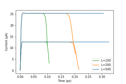
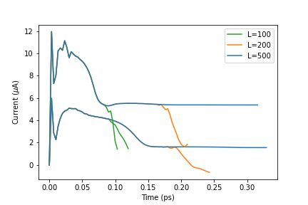
Numerical simulations were performed for numerous different parameters. For a given set of parameters, we calculate the mean current by disregarding transients and specifically averaging the current over the course of in the steady regime, i.e., in the time interval in which the current change is negligible. For practical purposes, we say the current change is negligible when it deviates by less than over . See Fig. 1(b). In practice, the steady regime exists for a finite interval of times depending on the sizes of the reservoirs, which are directly tuned by the parameter . This can be seen in Fig. 2, where the length of the steady regime always increases with respect to and would be stationary for all sufficiently large times in the limit . We do not provide here a mathematical proof of this conjecture, but this feature was present in all our numerical computations.
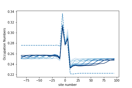
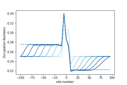
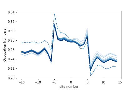
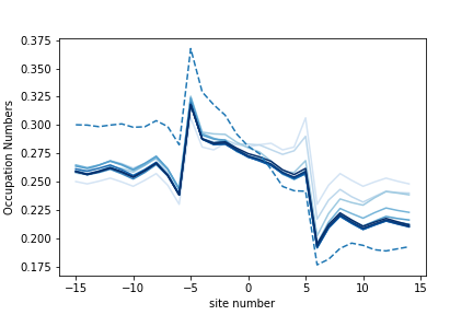
In fact, our numerical computations inevitably induce finite size effects. This can be well understood via the depletion of charge carriers in the finite reservoirs, which yield a current collapsing as seen in Fig. 2 for finite and sufficiently large times. This depletion is explicitly demonstrated in Fig 3 which gives the fermionic occupation number
| (22) |
at time in each lattice site in the band . One can observe that the depletion of the occupation number is directly correlated to the collapsing of the current, as expected with a naive classical viewpoint.
5.2 Emergence of Semi-Conductors
Although the experiments performed in [32] show that a set of protein-ligand complexes display Ohm-like conductivity (i.e. possibly via the formation of new molecular bonds that give rise to delocalized electronic states akin to conductors) we also predict formation of semi-conductor type characteristics. Although this has not been experimentally observed so far, our model predicts the existence of protein-ligand complexes with such a behavior, as anticipated for this kind of model. This is achieved by first noticing that the two bands in the model are linked with each other via the terms
for all lattice sites inside the system of lattice number (corresponding to a 1D quantum system of length , being the lattice spacing in ), see (6). The parameter allows us to control the nature of the conductor.
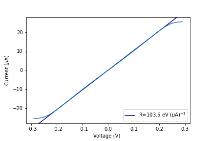
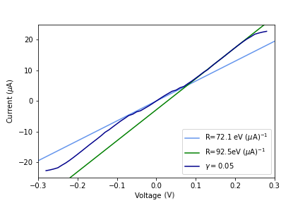
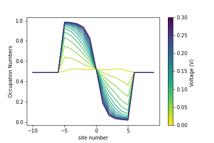
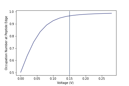
For , the two bands are disconnected and the system behaves as a regular conductor. In particular, the current increases linearly with voltage for sufficiently small electric potentials. This behavior is seen for and the same behavior holds true for small , see, e.g., Fig. 4(a). All these phenomena are of course expected and can in fact be mathematically showed in great generality, see, e.g., [7, 6], even in the limit of infinitely large .
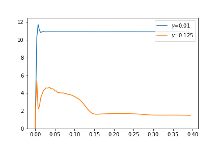
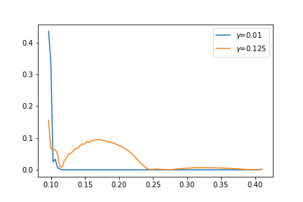
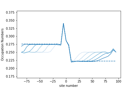
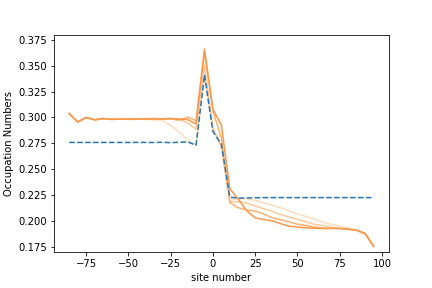
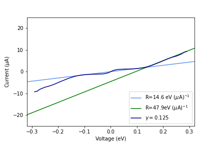
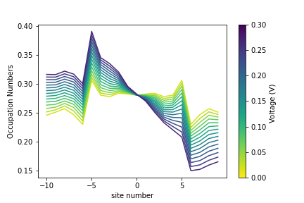
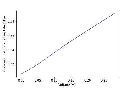
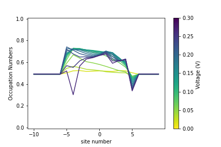
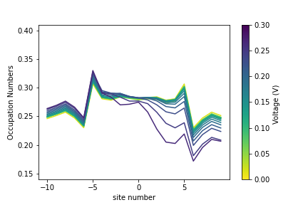
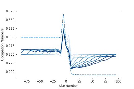
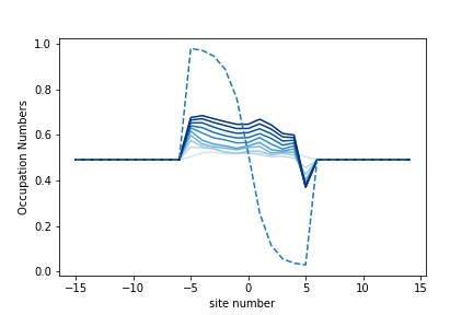
For the linear relationship between current and voltage progressively disappears as the average resistivity increases at lower voltages. The origin of this behavior can be studied by looking at the occupation numbers of the different lattice sites for the limit Gibbs state at different values of , see Figure 5. For non-zero gamma as increases the occupation numbers for the limit Gibbs state in the non-conducting band also increase. As this insulating band becomes saturated at the lattice-sites, the 1D quantum system once again starts to act as a conductor. For sufficiently strong , this phenomenon starts to be visible in terms of the charge transport within the (conducting) band 1:
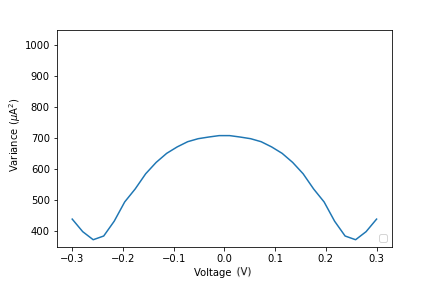
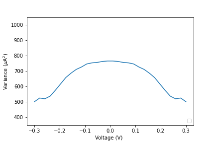
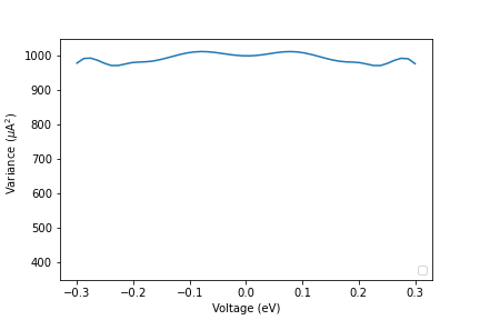
In Figure 5(b), we anticipate a change of current response at a saturation voltage of approximately , which is precisely the case, as shown in 4. In fact, at the system starts to exhibit this semi conductor-like behavior, see Figures 4(c) and 4(e). This behavior is concomitant with the current fluctuations given in Figs. 4(b)–4(f): The high electric resistance for small voltages is associated with an increase of the current fluctuations until some saturation regime (corresponding to the voltage threshold) from which the fluctuations decrease again, as in the conductor case. Note that the current fluctuations once again increase in any case for sufficiently large voltage beyond the linear (resp. piece wise linear) regime in the conductor (resp. semi-conductor) case.
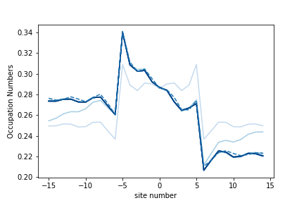
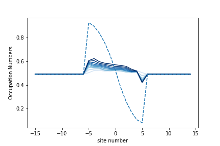
To complement this discussion, Figs. 6 shows the difference between the semiconductor () and conducting cases () in terms of time-dependent occupation numbers, at a fixed . In this last case, the second band inside the 1D-quantum system is slightly time dependent, in contrast with the trivial case . But, the effects of the band 0 on currents are negligible while they significantly alter the transport properties at , as explained above. The saturation phenomenon leading to the semi-conductor like behavior can also be seen by comparing Figs. 6(a), 6(c), 6(e) for and with Fig. 7(c) for the same but at , keeping in mind Fig 4(e).

5.3 Dependence on the Length of the System
In 2012, the accuracy of the macroscopic laws of charge transport have been shown for nanowires (of a few nanometers scale) of Si doped with phosphorus atoms, even at very low temperature (4.2 K) [1]. This implies that quantum effects can vanish extremely rapidly with respect to growing space scales.
From a mathematical perspective, the expectation of microscopic current densities with respect to growing space scales converges, as proven in [16, 6]. Furthermore, quantum uncertainty of microscopic electric current densities around their (classical) macroscopic value decays exponentially fast with respect to the volume of the region of the lattice where an external electric field is applied. This was specifically shown for non-interacting lattice fermions with disorder (one-band, any dimension) [25, 17].
Our model does not have any random external potential, but two bands inside the system of length , which corresponds in our unit to
see Section 3.3. Therefore, we analyze how fast the convergence of the current density converges to a fixed value.
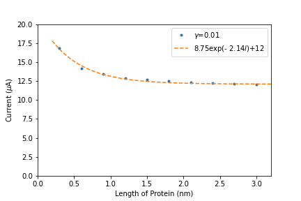
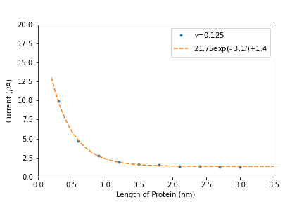
In Fig. 8, we confirm the exponential convergence of the current density to a fixed value as conjectured from [25, 17]. In particular, in these numerical experiments, is already a large quantum object in the sense that the limit point is already reached. Note, finally, that the semiconductor and conductor cases have the same behavior with respect to such convergences.
5.4 Dependence on Temperature
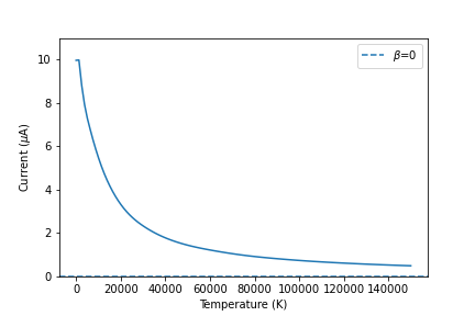
The energy scale used here are of the order of tenth of volts electronvolts. This is coherent with the voltage applied in the experiments described in [32]. In this energy scale, a room temperature, i.e., , corresponding to an inverse temperature , already refers to a very low temperature regime. Consequently, the transport properties of the system are basically independent of temperatures below room temperatures.
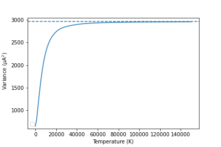
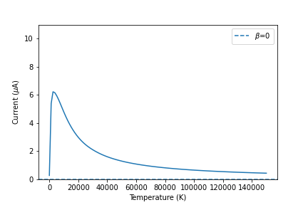
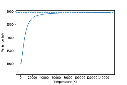
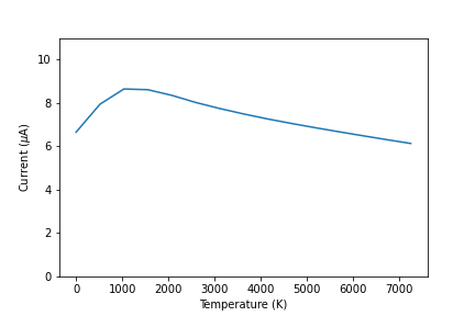
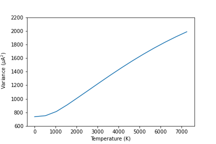
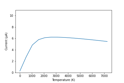
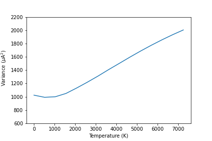
On the one hand, this is coherent with observations done in [18] on charge transport in some 1D quantum system. On the other hand, the energy scale used here may be inaccurate in many situations. We therefore explain the behavior of the model in the high temperature regime, which basically refers to , even if it corresponds to nonphysical temperatures () in our energy scale. This is performed in Fig. 9, showing an expected decrease of currents (equivalently an increase of the electric resistance) as the temperature increases. This is true for all regimes (conductor and semi-conductor). In the same way, the variance increases with the temperature, since thermal fluctuations are of course added to the purely quantum ones. See Fig. 9.
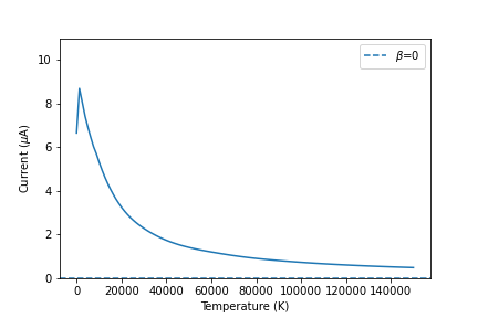
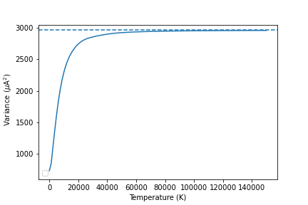
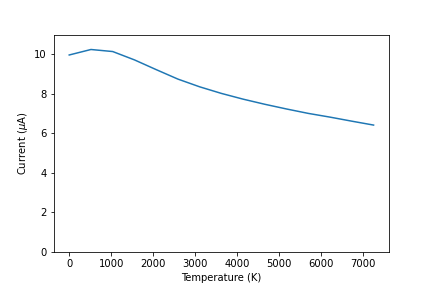
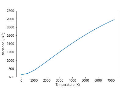
In contrast with the case with no insulating band 0, the two-band system has very interesting behavior for small temperatures: The current fluctuations are basically increasing, as naively anticipated, except in the semi-conductor regime for small temperatures. See Fig. 10. Remarkably, the current reaches a maximum value for some non-zero temperature before decreasing to zero in the limit . See again Figs. 9 and 10. It means in this case that the first excited state of the model interestingly favors the existence of currents, as compared with the ground states. It seems that this occurs for all and this effect increases with to the point that even the current variance starts to become non-monotone. This is a non-trivial information on the spectral properties of the model.
6 Conclusion
A first modelling attempt, based on many-body (fermionic) quantum statistical principles, is given to explain how Ohm’s law emerges in long-range charge transport within protein-ligand complexes, the conductances of which have been measured in aqueous solutions and via STM and Pd substrate [32]. To this end, we build upon the mathematically rigorous framework (explored by one of the authors and collaborators), which provides proof for the convergence of the expectations of microscopic current densities and also crucially explains how the microscopic (quantum) effects on charge transport vanishes with respect to growing space scales [6, 16]. This is coherent with [17, 25] showing the exponentially fast (with respect to growing scales) disappearance of quantum effects on electric currents for non-interacting lattice fermions with disorder (one-band, any dimension) [17, 25].
This leads us to propose for the protein-ligand complexes a simple quasi-free two band lattice model described via the second quantization formalism, where the non-conducting band attempts to capture the possibility that fermions may become trapped (via a hopping term, similar to a classic semi-conductor). Noteworthy, the model does not consider aqueous environment (natural to proteins) since the experiments we seek to explain were undertaken in an electrical potential region where ion current flows are not expected (i.e. no charge transfer is anticipated) [32]. By fixing physiological parameter sets (although not all microscopic parameters are available due to the novelty of these experiments) we then study the charge transport of our nanometric quantum protein-ligand system in a mathematically rigorous way, without approximations (up to numerical precision) or a priori assumptions. The behavior of charge transport given here is therefore perfectly reliable, without any possible discussion up to the original definition of the model. Ultimately, we show how charge transport in a protein-ligand complex (modelled as a two-band lattice quantum system) leads to the emergence of Ohm-like law, therefore providing a tentative explanation for the experiments in [32]. We also show that there is exponentially fast convergence of the expectations of microscopic current densities. This should be related to the existence of non-vanishing current variance of linear response currents, consistent with previous studies under natural conditions on the (random) disorder [17, 25]). We expect that this is also true also for several-band models.
Admittedly however, the model’s voltage-current curve exhibits a discrepancy of several orders of magnitude when compared to that of the experiment. Specifically, the voltage applied in the experiments described in [32] is of the order of tenth of volts and the systems remains in the linear response regime. If this is correct, then the energy scales of the model should be of the same order. This yields a quantitative discrepancy since the rigorously computed currents are of the order of (see Figs. 4(a)–4(f)), whereas the measured currents in [32] are of the order of , times smaller. This issue cannot be a priori solved by reducing the hopping strength between the reservoirs and the band of the 1D quantum object (1D quantum system). Preliminary numerical computations show that the value of has to be extremely small to reduced the current by orders of magnitude, at the cost of almost isolating the 1D quantum system from the reservoirs and destroying the main transport properties described here.
Since there is no approximations or a priori assumptions on the model, there is probably an issue related to all the energy scales, meaning that the voltage seen by the protein/peptide is far less than tenth of volts. On the other hand, lower energy scales change the meaning of the low temperature regime, which may be in contradiction with previous results [18]. See discussions in Section 5.4.
Several reasons could be behind this discrepancy, to list a few:
-
1.
This may indicate that there is underlying biophysical phenomenon that the present model does not capture, which we will investigate in future works;
-
2.
This could be related to the aqueous environment surrounding the peptide/protein-ligand complexes enabling charge transfer, although the original experiments claim otherwise [32];
-
3.
While we did investigate a range of parameter regions, there is still the possibility that some parameters could be far off.
Nevertheless, our framework provides a novel approach to study rigorously charge transport (under quantum and thermal fluctuations) and to understand the breakdown of the classical (macroscopic) conductivity theory at microscopic scales. The theory can be applied to both biological transport and other physical systems and in this sense it is a unifying approach. In particular, the theory allows us to explain the emergence of electronic states that are delocalized within a protein/peptide or physical systems. Hence we provide predictions for both conducting and semi-conducting like properties, although semi-conductor type characteristics has not yet been observed since only six protein-ligand complexes have been tested so far [32]. Nevertheless, these predictions could be tested in future experiments. The basic nature of the model allows it to be readily adjusted to explore a variety of different phenomena. For instance, an external potential such as
with being some (i.i.d.) random variables (cf. the Anderson model), could have been considered without breaking the quasi-free property of the model. This term can be used to verify and study the linear dependence of the resistivity with respect to the length of the 1D quantum system (another version of Ohm’s law). Note indeed that this property on the resistivity does not hold true for our two-band model (like for the one-band one, i.e., for ), since the current does not seem to vanish in the limit of infinite (Fig. 8) while it is expected [25, 17] to be equal to the macroscopic one at relatively small lengths .
In the immediate future we will investigate the discrepancy of the model (as explained above) and we will study the emergence of the telegraph noise as observed in the protein-ligand complex experiments (see [32, Fig. S7]). Presently, as far as we know, there is no theory based from first principles of Quantum mechanics to explain telegraph noise. Current theories are mainly phenomenological, modelled via a (Markovian continuous-time) stochastic process that jumps discontinuously between two distinct values, as it is shown for currents in [32, Fig. S7]. The telegraph noise is in particular characterised by a bimodal distribution of currents. Since this can be characterised via some statistical methods involving higher moments (like the kurtosis and skewness) besides the variance, our approach can be used to understand the appearance of the telegraph noise via a purely quantum microscopic theory.
In the future, it will be interesting to develop theories to explain long-range (micrometer-scale) conduction through peptides/proteins and through supramolecular structures, such as coiled-coils, -sheets, -helices, collagen, or elastin mimics etc. This is important because the molecular and organic electronics community are currently developing systems that merge conjugated molecules with amino acids, which form electronically delocalized supramolecular structures that facilitate long-range charge transport. Thus a theory that supports this will be fundamentally interesting and potentially significant for the development of bioelectronic materials. The limiting factor of our proposed framework is the rapid increase in computational complexity for systems with higher dimensions.
Finally, our code is freely accessible at:
https://github.com/RoisinMary/quasifree_chargetransport.git and can readily run in a standard computer (e.g. we run it on a MacBook Pro with a 2,4 GHz Quad-Core Intel Core i5-processor).
7 Acknowledgment
J.-B. Bru is supported by the Basque Government through the grant SR, JBB and RB acknowledge support from Ikerbasque (The Basque Foundation for Science), and the Basque Government through the BERC 2022-2025 program and by the Ministry of Science and Innovation: BCAM Severo Ochoa accreditation CEX2021-001142-S / MICIN / AEI / 10.13039/501100011033. SR further acknowledges of the RTI2018-093860-B-C21 funded by (AEI/FEDER, UE) and acronym “MathNEURO”. JBB meanwhile acknowledges of the grant PID2020-112948GB-I00 funded by MCIN/AEI/10.13039/501100011033 and by ”ERDF A way of making Europe”, as well as the COST Action CA18232 financed by the European Cooperation in Science and Technology (COST). JUA aknowledges support from the Spanish Government, grants PID2020-117281GB-I00 and PID2019-107444GA-I00, partly from European Regional Development Fund (ERDF), and the Basque Government, grant IT1483-22.
8 Appendix
The quasi-free nature of the model allows a significant reduction of the dimension for the numerical calculation. In this appendix we shortly recall the necessary theory for the convenience of the reader.
8.1 The One-particle Picture
We use the algebraic formulation of quantum many-body problems, which is, from a conceptual point of view, the natural one, as the underlying physical system is many-body. Moreover, it has some advantageous technical aspects, both specific (like the possibility of using Bogoliubov-type inequalities in important estimates) and general ones (like the very powerful theory of KMS states). However, in the present paper we only deal with non-interacting fermions and in this specific example, one can equivalently use the one-particle picture, as explained in detail in [25, Section C.3].
For instance, the Hamiltonian defined on the fermionic Fock space (2) is the second quantization of the following one-particle Hamiltonian acting on the one-particle Hilbert space (1): Let be the usual 1D-discrete Laplacian defined on by
| (23) |
We consider a conducting band and an insulating band as well as spinless fermions. Thus, the one-particle Hilbert space (1) is in this case equal to
In particular, if then corresponds to the insulating band , while refers to the conducting band . For any set , we define the orthogonal projection from to . For any , let and fix with .
Then, the Hamiltonians
are the second quantization of the one-particle Hamiltonians
respectively. All other quantities defined in Section 3, including current observables (see [25, Section C.3]), can be written as the “second quantized” version of one-particle objects, like the velocity operator in the case of currents. This is possible because all our quantities are related to operators that are quadratic in the fields.
8.2 CAR –Algebras
In the algebraic formulation of fermion systems, the CAR –algebra associated with a Hilbert space , denoted by , is the –algebra
generated by a unit and a family of elements satisfying Conditions (a)–(b):
(a) The map is (complex) linear.
(b) The family satisfies the
Canonical Anticommutation Relations (CAR): For all ,
| (27) |
If is finite dimensional then it is well-known that is –isomorphic to the –algebra of all bounded linear operators acting on the fermionic Fock space constructed from . In particular,
| (28) |
see (10)–(11). Note that for infinite-dimension Hilbert spaces , making the algebraic approach more general. In particular, . See, e.g., [15] for more details.
Note that the creation and annihilation operators in the definitions of Hamiltonians in Section 3 correspond to
| (29) |
for each lattice site and band , where is the canonical orthonormal basis of defined by for all and .
8.3 Quasi-Free States
Gauge-invariant quasi-free states on a CAR –algebra are positive and normalized linear functionals such that, for all and ,
| (30) |
if , while in the case ,
| (31) |
See, e.g., [2, Definition 3.1], which refers to a more general notion of quasi-free states. The gauge-invariant property corresponds to (30), whereas [2, Definition 3.1, Condition (3.1)] only imposes the quasi-free state to be even, which is a strictly weaker property than being gauge-invariant.
Quasi-free states are therefore particular states that are uniquely fixed by two-point correlation functions. In fact, a quasi-free state is uniquely defined by its so-called one-particle density matrix of the state , which is defined through the conditions
| (32) |
Note that satisfies .
Since the full Hamiltonian (see (9) and (28)) is the second quantization of an explicit one-particle Hamiltonian
acting on the one-particle Hilbert space (11), one proves that the Gibbs state (12) is a quasi-free state with one-particle density matrix equal to
| (33) |
at fixed inverse temperature . See, e.g., [24, Section 2.3]. In particular, all correlation functions of the many-fermion system can be numerically computed within the one-particle Hilbert space , thanks to (30)–(31) and (33).
8.4 Quasi-Free Dynamics
In the algebraic formulation of quantum mechanics (cf. the Heisenberg picture), dynamics occur in a CAR –algebra, via a strongly continuous group of –automorphisms of . A quasi-free dynamical system associated with a one-particle Hamiltonian acting on is a strongly continuous group of –automorphisms of uniquely defined by the conditions
The time evolution of a state is given by in the Schrödinger picture of quantum mechanics. If the dynamics and the state are both quasi-free then, for all times , is a quasi-free state with one-particle density matrix equal to
In other words, is the solution to the Liouville equation in the one-particle Hilbert space .
Define now the Hamiltonian by
for and natural numbers , where is the operator defined, for any and , by
being the characteristic function of a set . The Hamiltonian can again be seen as an operator acting on the one-particle Hilbert space (11). In the present paper, the dynamics is defined by (14) on either or for natural numbers . Since the full Hamiltonian (see (13)) with electric potentials is the second quantization of , one proves that the dynamics (14) is quasi-free:
| (34) |
See, e.g., [24, Section 2.3]. In particular, the Gibbs state (12) evolves in the Schrödinger picture within the set of quasi-free states and all physical quantities can be deduced from one-particle considerations. In this paper, we take advantage of this fact to significantly reduce the complexity of the calculations.
8.5 Example of Current Densities
Recall that elementary current observables are defined by (18), that is,
| (35) |
for natural numbers , and . Therefore, by using (29) and (32)–(34), we can compute its expectation in the Gibbs state at time as follows:
| (36) |
for natural numbers , , and . Using this formula and an explicit formulation of the one-particle Hamiltonian , we compute the expectation (20) of the current density observable defined by (19).
In order to calculate the variance
| (37) |
of this current, we additionally use Equation (31) in the following case:
| (38) |
for any , because the Gibbs state is quasi-free.
8.6 Discussion of the Implementation
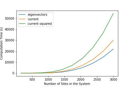
Here computations were performed to find the variance but the code can easily be extended to compute higher moments which could be instrumental in identifying, for example, a bi-modal distribution which is characteristic of telegraph noise. Code automatically implementing the simplifying CAR relations significantly reduces the difficulty of computing higher-order moments. However, because of the increasing number of linear operations needed such calculations can become expensive for large (see Fig. 11).
References
- [1] B. al. “Ohm’s Law Survives to the Atomic Scale” In Science 335.6064, 2012, pp. 64–67
- [2] H. Araki “On Quasifree States of CAR and Bogoliubov Automorphisms” In Publ. RIMS, Kyoto Univ. 13, 1971, pp. 385–442
- [3] P Becker and G Mana “The Lattice Parameter of Silicon: A Survey” In Metrologia 31 IOP Publishing, 1994, pp. 203–209
- [4] David N. Beratan et al. “Charge Transfer in Dynamical Biosystems, or The Treachery of (Static) Images” In Accounts of Chemical Research 48.2, 2015, pp. 474–481
- [5] Jochen Blumberger “Recent Advances in the Theory and Molecular Simulation of Biological Electron Transfer Reactions” In Chemical Reviews 115.20, 2015, pp. 11191–11238
- [6] J.-B. Bru and W. Siqueira Pedra “From the 2nd Law of Thermodynamics to the AC-Conductivity Measure of Interacting Fermions in Disordered Media” In Math. Models Methods Appl. Sci. 24.14, 2015, pp. 2587–2632
- [7] J.-B. Bru and W. Siqueira Pedra “Microscopic Conductivity of Lattice Fermions at Equilibrium – Part II: Interacting Particles” In Lett. Math. Phys. 106.1, 2016, pp. 81–107
- [8] J.. Burroughes et al. “Light-emitting diodes based on conjugated polymers” In Nature 347.6293, 1990, pp. 539–541
- [9] Mark Elbing et al. “A single-molecule diode” In Proceedings of the National Academy of Sciences 102.25, 2005, pp. 8815–8820
- [10] D.. Ferry “Ohm’s Law in a Quantum World” In Science 335.6064, 2012, pp. 45–46
- [11] R.E. Gleason “How far will circuits shrink?” In Science Spectra 20, 2000, pp. 32
- [12] C Groves “Simulating charge transport in organic semiconductors and devices: a review” In Reports on Progress in Physics 80.2 IOP Publishing, 2016, pp. 026502 DOI: 10.1088/1361-6633/80/2/026502
- [13] N. Hush “Adiabatic Rate Processes at Electrodes. I. Energy‐Charge Relationships” In J. Chem. Phys. 28, 1958, pp. 962–972
- [14] Nicole L. Ing, Mohamed Y. El-Naggar and Allon I. Hochbaum “Going the Distance: Long-Range Conductivity in Protein and Peptide Bioelectronic Materials” In The Journal of Physical Chemistry B 122.46, 2018, pp. 10403–10423
- [15] W. Siqueira Pedra J.-B. “Lieb-Robinson Bounds for Multi-Commutators and Applications to Response Theory” In SpringerBriefs in Mathematical Physics 13 Springer, 2017
- [16] W. Siqueira Pedra J.-B. and C. Hertling “AC-Conductivity Measure from Heat Production of Free Fermions in Disordered Media” In Arch. Ration. Mech. Anal. 220.2, 2016, pp. 445–504
- [17] W. Siqueira Pedra J.-B. and A. Ratsimanetrimanana “Quantum Fluctuations and Large Deviation Principle for Microscopic Currents of Free Fermions in Disordered Media” In Pure and Applied Analysis 2.4, 2020, pp. 943–971
- [18] W. Siqueira Pedra J.-B. and A. Ratsimanetrimanana “Solid-State Electron Transport via the Protein Azurin is Temperature-Independent Down to 4 K” In J. Phys. Chem. Lett. 11, 2020, pp. 144–151
- [19] D. Leeuw “Plastic Electronics” In Physics World, 1999, pp. 31
- [20] Dalton LR, Sullivan PA, Bale DH and Bricht BC “Theory-inspired nano-engineering of photonic and electronic materials: Noncentro symmetric charge-transfer electro-optic materials” In Solid-State Electronics 51.10, 2007, pp. 1263–1277 DOI: 10.1016/j.sse.2007.06.022
- [21] M.G.Kanatzidis “Conductive Polymers” In Chem. Eng. News 3, 1990, pp. 36
- [22] R.. Marcus “Electrostatic Free Energy and Other Properties of States Having Nonequilibrium Polarization. I” In J. Chem. Phys. 24.5, 1956, pp. 979–989
- [23] R.. Marcus “On the Theory of Oxidation-Reduction Reactions Involving Electron Transfer. I” In Journal of Chemical Physics, 24.5, 1956, pp. 966–978
- [24] W. Siqueira Pedra N… and L….. Müssnich “Large Deviations in Weakly Interacting Fermions - Generating Functions as Gaussian Berezin Integrals and Bounds on Large Pfaffians” In Rev. Math. Phys. 34.1 World Scientific, 2022, pp. 2150034
- [25] W. Siqueira Pedra N… and A. Ratsimanetrimanana “Accuracy of Classical Conductivity Theory at Atomic Scales for Free Fermions in Disordered Media” In J. Math. Pures Appl. 125 Elsevier Masson SAS, 2019, pp. 209–246
- [26] S-Y Sheu, D-Y Yang, HL Selzle and EW Schlag “Charge transport in a polypeptide chain” In The European Physical Journal D-Atomic, Molecular, Optical and Plasma Physics 20.3 Springer, 2002, pp. 557–563
- [27] Sheh-Yi Sheu, Edward W Schlag and Dah-Yen Yang “A model for ultra-fast charge transport in membrane proteins” In Physical Chemistry Chemical Physics 17.35 Royal Society of Chemistry, 2015, pp. 23088–23094
- [28] Hideki Shirakawa et al. “Synthesis of electrically conducting organic polymers: halogen derivatives of polyacetylene, (CH)” In J. Chem. Soc., Chem. Commun. 16, 1977, pp. 578–580
- [29] Miriam Valle, Rafael Gutiérrez, Carlos Tejedor and Gianaurelio Cuniberti “Tuning the conductance of a molecular switch” In Nature Nanotechnology 2.3, 2007, pp. 176–179
- [30] R. Wesche “Physical Properties of High-Temperature Superconductors” In Wiley series in materials for electronic and optoelectronic applications Wiley, 2015
- [31] Shihai Yan et al. “Computational studies on electron and proton transfer in phenol-imidazole-base triads” In Journal of computational chemistry 31.2 Wiley Online Library, 2010, pp. 393–402
- [32] Bintian Zhang et al. “Role of contacts in long-range protein conductance” In Proceedings of the National Academy of Sciences 116.13 National Acad Sciences, 2019, pp. 5886–5891