Key Feature Replacement of In-Distribution Samples for Out-of-Distribution Detection

Abstract

Out-of-distribution (OOD) detection can be used in deep learning-based applications to reject outlier samples from being unreliably classified by deep neural networks. Learning to classify between OOD and in-distribution samples is difficult because data comprising the former is extremely diverse. It has been observed that an auxiliary OOD dataset is most effective in training a “rejection” network when its samples are semantically similar to in-distribution images. We first deduce that OOD images are perceived by a deep neural network to be semantically similar to in-distribution samples when they share a common background, as deep networks are observed to incorrectly classify such images with high confidence. We then propose a simple yet effective Key In-distribution feature Replacement BY inpainting (KIRBY) procedure that constructs a surrogate OOD dataset by replacing class-discriminative features of in-distribution samples with marginal background features. The procedure can be implemented using off-the-shelf vision algorithms, where each step within the algorithm is shown to make the surrogate data increasingly similar to in-distribution data. Design choices in each step are studied extensively, and an exhaustive comparison with state-of-the-art algorithms demonstrates KIRBY’s competitiveness on various benchmarks.

Introduction

Out-of-distribution (OOD) detection is important in safety-critical applications where predictions should not only be accurate on average, but also reliable. Deep neural networks (DNNs) excel at classifying samples drawn from a distribution matching the training set’s, but they also tend to inaccurately classify out-of-distribution (OOD) data with high confidence even when the samples deviate significantly from the training distribution (Hendrycks and Gimpel 2017; Liu et al. 2020a). In order to prevent classifiers from producing such predictions, safety-critical applications use OOD detection to alert the user when it is likely that the DNN cannot reliably classify a given input (Cao et al. 2020; Feng, Rosenbaum, and Dietmayer 2018; Filos et al. 2020).

Denote $\mathcal{X}$ to be the set of all possible, including undesirable, input images to a classifier. An in-distribution (ID) is the distribution from which a training set is sampled. Its support is described as an ID set $\mathcal{X}_{\text{ID}}\subset\mathcal{X}$, and OOD data $\mathcal{X}_{\text{OOD}}$ is any data that is unlikely to be drawn from this ID. The task of detecting OOD samples is a binary hypothesis test

$$\Psi\left(x\right)=\begin{cases}0&\text{if }x\in\mathcal{X}_{\text{ID}}\\ 1&\text{if }x\in\mathcal{X}_{\text{OOD}}\end{cases}$$ (1)

where the main difficulty lies in $\mathcal{X}_{\text{OOD}}$ being too large to be represented by any reasonable dataset size.

Figure 1: Examples of our auxiliary OOD dataset constructed from STL-10 (Coates, Ng, and Lee 2011). Each column represents raw images, activation maps, and OOD constructions, respectively.

In this paper, we primarily focus on methods to detect OOD samples without having to modify a classifier trained on ID data $\mathcal{X}_{\text{ID}}$. Having to (re-)train a model specifically for OOD detection on a large training set is computationally demanding, and classification performance may be adversely affected (Van Amersfoort et al. 2020). Instead, we describe a method to construct an auxiliary dataset of surrogate OOD data from any training (ID) set.

Our work builds upon the observation that OOD samples used to learn a decision rule $\Psi$ are most effective when they are semantically similar to ID samples (Lee et al. 2018a). First, we establish that OOD samples are perceived by a DNN to be semantically similar to ID samples when they share a common background. Then we propose a procedure to construct an auxiliary OOD ‘rejection” set by replacing class-discriminative features of a training set with marginal background features (see Figure 1). A shallow rejection network $\hat{\Psi}$ operating on a pre-trained classifier’s latent space can then be trained on the training (ID) and auxiliary OOD datasets to detect OOD data.

Numerical experiments confirm that our procedure indeed generates surrogate OOD data close to ID examples. Accordingly, a rejection network trained on this construction outperforms state-of-the-art OOD detection algorithms on most benchmarks. The benefits of our method are that (1) the OOD dataset is constructed offline while being adaptive to any ID training data; (2) its resultant dataset is “close” to ID data which is observed to impact OOD detection performance; (3) a classification network need not be re-trained. Furthermore, our method does not rely on an “oracle” access to a subset of OOD samples. This contrasts other OOD detection algorithms whose performance degrades when a subset of real OOD data is unavailable (Hsu et al. 2020; Shafaei, Schmidt, and Little 2019).

Figure 2: Average top-10 confidences of a CIFAR-10 classifier tested on CIFAR-100 data whose classes are listed in rows. For example, a “sea” image from CIFAR-100 is classified as “ship” with $\approx 0.6$ confidence. Each star ($\star$) indicates an OOD class (CIFAR-100) that has a similar ID background and more results with other ID classes are in Appendix A.

Figure 3: OOD samples drawn from right OOD classes are classified as left ID classes with high confidence (MSP) when backgrounds overlap substantially, demonstrating the inadequacy of MSP for OOD detection.

Related Work

Post-hoc algorithms are those that do not require modifying a pre-trained classifier to detect OOD samples. The simplest post-hoc algorithm thresholds the classifier’s maximum softmax probability (MSP) to detect OOD samples (Hendrycks and Gimpel 2017). A substantial improvement was achieved by ODIN (Liang, Li, and Srikant 2018), where controlled noise is added to test samples and temperature scaling is applied to better separate predictions on ID and OOD samples. Treating the latent space of pre-trained models as class-conditional Gaussian variables, Lee et al. (2018b) uses the Mahalanobis distance with sample mean and covariances as a rejection rule. Used either as a post-hoc or fine-tuning method, Energy (Liu et al. 2020b) maximizes the log-sum-exp potential to calibrate classifiers (Grathwohl et al. 2020) whose confidence can then be used to detect OOD cases. ReAct (Sun, Guo, and Li 2021) suggests truncating the high activations to address distinctive patterns arising when processing OOD data. DICE (Sun and Li 2022) is a sparsification technique which ranks weights by contribution, and then uses the most significant weights to reduce noisy signals in OOD data.

Post-hoc methods usually require tuning a parameter on a small subset of OOD data. Depending on the application, using a subset of true OOD data may be impractical. Except for MSP and Energy described above, other methods specify parameter(s) that must be tuned on a reserved OOD subset.

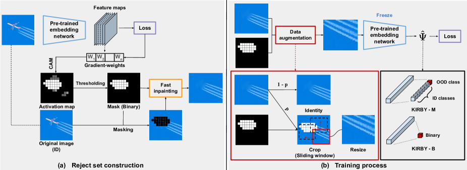
Figure 4: Diagram of KIRBY. (a) Training images are fed into a pre-trained model to locate and erase key ID class-discriminative features. A rejection set is then constructed by inpainting the erased images with marginal features. (b) A rejection network $\hat{\Psi}$ is trained to classify ID and OOD samples, implemented as either KIRBY-M where a multi-class classifier is trained to classify all $K$ classes in the ID set in addition to the OOD class, or KIRBY-B where a binary classifier differentiates ID vs. OOD.

Closest to our work are algorithms that train a rejection network on surrogate OOD data. Outlier Exposure (OE) (Hendrycks, Mazeika, and Dietterich 2019) uses a static dataset independent of ID samples by distilling the “80 Million Tiny Images” dataset (Torralba, Fergus, and Freeman 2008) and excluding ID samples. CEDA and ACET (Hein, Andriushchenko, and Bitterwolf 2019) both use random noise and pixel shuffling of ID samples, the latter including an adversarial enhancement procedure. An analysis in (Lee et al. 2018a) reveals that synthetic examples are most useful as OOD surrogates when they lie near ID examples, and the authors train a classifier with an additional Kullback-Leibler (KL) penalty enforcing uniform predictions on OOD images generated by a generative adversarial network (GAN; Goodfellow et al. 2014).

Excessively distant synthetic examples from ID samples may not help with OOD detection because easy-to-learn outlier features can be discriminated rather trivially. As described earlier, OOD detection is difficult because the set of OOD samples cannot be covered entirely. A desirable trait in constructing reject sets is to carefully generate images that do not contain ID classes but are sufficiently close to effectively train a rejection network. This concept will be revisited later, where the proposed algorithm is shown to satisfy the above trait.

Method

Motivation and Empirical Evidence

It has been repeatedly observed that surrogate OOD data is most effective when nearby ID data (Hein, Andriushchenko, and Bitterwolf 2019; Hendrycks, Mazeika, and Dietterich 2019; Lee et al. 2018a; Ren et al. 2019). Conversely, surrogate data far from ID examples hardly affect OOD detection performance (Hendrycks, Mazeika, and Dietterich 2019). This limitation of distant rejection classes is especially evident when OOD detection is evaluated on a set close to ID examples (Hein, Andriushchenko, and Bitterwolf 2019).

Ren et al. (2019); Ming, Yin, and Li (2022) suggest that neural networks incorrectly classify OOD samples with high confidence when their background overlaps with ID examples. To complement their observation, we trained a WideResNet (Zagoruyko and Komodakis 2016) on CIFAR-10 (Krizhevsky 2009) and plot the average confidence (bars) of predictions on OOD samples (row) that are classified as respective classes in Figure 2. For example, “Mountain” images are on average classified as “Airplane” with confidence $\approx 0.4$ whereas $0.1$ is ideal. Here we observe that softmax confidence scores on OOD classes marked with stars are high when ID classes contain similar background images (see Figure 3).

Based on these observations, we propose a Key In-distribution feature Replacement BY inpainting (KIRBY) procedure to construct surrogate OOD data $\tilde{\mathcal{X}}_{\text{OOD}}$ from ID samples by marginalizing their key representative features with their marginal background features. A shallow rejection network $\hat{\Psi}$ attached to the pre-trained classifier’s layer preceding global average pooling (GAP) is then trained to classify ID samples and the auxiliary OOD dataset.

Out-of-Distribution Set Construction

Let $x\in\mathcal{X}_{\text{ID}}$ be a classifier’s input of training samples and $y\in\mathcal{Y}=\{1,...,K\}$ be a label. To generate surrogate OOD samples, we first erase key features from ID training images:

$$\tilde{x}_{\text{OOD}}=x\odot\mathbf{M},$$ (2)

where $\odot$ is element-wise multiplication, and $\mathbf{M}\in\{0,1\}^{W\times H}$ is a binary mask indicating class-specific key regions. This mask is computed by thresholding the output $\mathbf{A}\in[0,1]^{W\times H}$ of any class activation map (CAM) algorithm (Zhou et al. 2016; Selvaraju et al. 2017):

$$\mathbf{M}_{ij}=\begin{cases}0&\text{if }\mathbf{A}_{ij}\geq\lambda,\\ 1&\text{otherwise,}\end{cases}$$ (3)

where $\lambda$ is the threshold that determines how many key features are erased.

Masked regions are then replaced by marginal features using the fast marching inpainting method (Telea 2004) to produce perceptually plausible OOD images. The overall pipeline of KIRBY is illustrated in Figure 4a. In the experimental results section, we will explore how choices of CAM and inpainting algorithms affect OOD detection performance.

WSOL CIFAR-10 CIFAR-100 STL-10 Average Method Block # Accuracy FPR $\downarrow$ AUROC $\uparrow$ FPR $\downarrow$ AUROC $\uparrow$ FPR $\downarrow$ AUROC $\uparrow$ FPR $\downarrow$ AUROC $\uparrow$ Smooth-Grad (Smilkov et al. 2017) Input - 15.32 96.81 33.92 91.87 71.97 79.25 40.40 89.31 Grad-CAM (Selvaraju et al. 2017) 1 53.99 17.67 96.33 37.38 90.90 52.30 87.45 35.78 91.56 2 18.36 95.96 37.91 91.09 49.37 88.34 35.21 91.79 3 14.27 96.96 33.39 92.41 44.92 89.10 30.86 92.82 Grad-CAM++ (Chattopadhay et al. 2018) 1 .56.42 22.98 94.79 38.92 90.72 53.84 87.10 38.58 90.87 2 20.59 95.65 42.13 89.92 50.68 87.77 37.80 91.11 3 14.02 97.04 34.15 92.18 44.95 89.47 31.04 92.89 Layer-CAM (Jiang et al. 2021) 1 57.83 20.72 95.47 40.65 90.08 53.23 87.37 38.20 90.97 2 19.72 95.75 40.34 90.34 50.34 88.02 36.80 91.37 3 14.01 97.03 33.64 92.31 44.85 89.50 30.83 92.86

Table 1: Influence of CAM variants and where features are activated on downstream OOD detection performance for KIRBY-M. Block # describes the block in WideResNet-40-2 at which CAM is applied. Listed WSOL accuracies are those reported in (Jiang et al. 2021) for ILSVRC (Russakovsky et al. 2015).

Training a Rejection Network

A rejection network $\hat{\Psi}$ is trained to classify between ID and (surrogate) OOD samples. This network can be either a binary classifier (KIRBY-B) or a multi-class classifier (KIRBY-M) that learns an OOD class in addition to the $K$ ID classes. For KIRBY-M, OOD predictions are obtained by thresholding the reject class at inference time.

When training this network, we augment the surrogate OOD set by randomly choosing to select the patch most distant from the inpainted area, in place of the original surrogate image. This patch is found with a sliding window that is $1/4$ the size of the original image. This procedure compensates for artifacts that may be introduced by inpainting, and is illustrated in Figure 4.

There are several benefits that come from our method. Instead of fine-tuning a pre-trained classifier, we attach the rejection network to the penultimate layer of the pre-trained classifier and train the rejection network to leave classification performance unaffected for samples that pass the OOD detection test. Compared to most post-hoc algorithms, our method does not require a small subset of the OOD set to tune hyper-parameters. This is critical in many practical applications where the source of OOD samples is unknown and cannot be sampled prior to deployment.

Experiments

Setup

Datasets

Following (Liang, Li, and Srikant 2018; Liu et al. 2020b), we test OOD detection performance using CIFAR-10 and CIFAR-100 as ID sets and the following OOD sets:

• SVHN (Netzer et al. 2011). This dataset consists of $32\times 32$ RGB images associated with digit ($0$–$9$) classes. We use 26,032 test images.

• Textures (Cimpoi et al. 2014) was designed as a basis for describable texture attributes, and contains 47 classes spanned across 5,640 images.

• LSUN-crop & LSUN-resize are released by authors from (Liang, Li, and Srikant 2018), where the Large-scale Scene UNderstanding dataset (LSUN, (Yu et al. 2015)) is processed with random crop and downsampling.

• Place-365 (Zhou et al. 2017) test set contains 900 photographs per (scene) class.

• iSUN (Xu et al. 2015) used for OOD detection contains 8,925 images constructed for eye tracking.

Additionally we test on STL-10 as ID with a larger resolution of $96\times 96$ where all OOD examples are re-sized accordingly. Specifically for both LSUN variants, we follow the procedure in (Liang, Li, and Srikant 2018) to obtain $96\times 96$ from the SUN test set instead of re-sizing from their cropped and downsampled versions.

Evaluation Metrics

Performance is measured with respect to the following standard criteria.

• FPR measures the false positive rate (FPR) at the operating point when a negative OOD example is mis-classified as a positive in-distribution sample with true positive rate (TPR) 95%. Lower is better.

• AUROC is the area under the receiver operating characteristic curve obtained by varying the operating point. Higher is better.

Training Details

A wide variety of modern network architectures were used to compare algorithms: WideResNet-40-2 (Zagoruyko and Komodakis 2016), DenseNet-BC (depth $L=100$, growth rate $k=12$) (Huang et al. 2017), and ResNet-34 (He et al. 2016). The rejection network is implemented as two fully-connected layers with its hidden layer’s width being $2048$. Training converges in 5 epochs using SGD-momentum with the initial learning rate of 0.01 and weight decay $5\times 10^{-4}$. The rejection network is optimized with cross-entropy loss. The threshold parameter $\lambda$ is set as $0.3$, and the augmentation that replaces an image with a patch is applied to each sample with probability $0.5$. 

Baselines

We compare our method with post-hoc methods: MSP (Hendrycks and Gimpel 2017), ODIN (Liang, Li, and Srikant 2018), Energy (Liu et al. 2020b), Mahalanobis (Lee et al. 2018b), ReAct (Sun, Guo, and Li 2021), and DICE (Sun and Li 2022) with their hyper-parameters found searching over grids suggested in respective references when necessary; MSP and Energy do not have parameters to tune. Likelihood-based methods (JEM; Grathwohl et al. 2020 and LR; Xiao, Yan, and Amit 2020) are also compared, where the input density $p\left(x\right)$ of a sample $x$ is modeled and used to derive the decision rule $\Psi$. JEM suffers from training instability, so we follow their experiments and use WideResNet-28-10 without BatchNorm (Ioffe and Szegedy 2015) and additionally report performance using WideResNet-40-2 (without BatchNorm). Lastly, we compare KIRBY with ACET (Hein, Andriushchenko, and Bitterwolf 2019) and GAN (Lee et al. 2018a) which directly learn a rejection rule from surrogate OOD samples as described earlier. Excluding post-hoc methods, we report averaged AUROC and FPR over five runs.

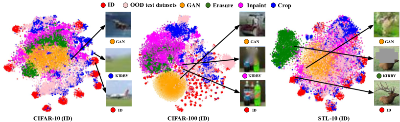
Figure 5: Visualization of proximity between auxiliary dataset constructions and ID samples using t-SNE (Van der Maaten and Hinton 2008). For each ID sub-figures, all six OOD test sets are used in the above illustration.

AUROC / FPR CIFAR-10 CIFAR-100 STL-10 w/o inpainting 95.30 / 23.03 88.81 / 41.22 84.28 / 55.10 Mean 96.59 / 15.82 92.07 / 34.05 87.34 / 50.58 CS 97.40 / 11.42 92.28 / 29.56 84.59 / 51.42 FM 97.03 / 14.01 92.31 / 33.64 89.50 / 44.85

Table 2: Effect of different inpainting methods on KIRBY-M’s OOD detection performance. We report AUROC and FPR averaged over OOD test sets.

Latency CIFAR-10 CIFAR-100 STL-10 CS 124.65 $\pm$ 1.32 134.65 $\pm$ 1.08 1566.87 $\pm$ 10.15 FM 2.11 $\pm$ 0.51 1.84 $\pm$ 0.23 8.85 $\pm$ 3.14

Table 3: Computation time (ms / example) comparison between inpainting methods, measured on an Intel(R) Xeon(R) Gold 5220 CPU.

Design Choices of KIRBY

We assess in Table 1 how the choice of saliency and inpainting methods affect OOD detection performance by experimenting with several CAM and inpainting algorithms. Additionally, we also show how the choice of layer (residual block) at which features are activated affects performance. Because saliency maps are often designed for weakly-supervised object localization (WSOL), the WSOL performance is also shown for reference.

We observe that WSOL accuracy is not a good indicator of how the saliency method used in KIRBY would affect OOD detection performance. Instead, the layer at which CAM is applied is much more important.

CAM Erasure Inpaint Crop CIFAR-10 CIFAR-100 STL-10 AUROC $\uparrow$ AUROC $\uparrow$ AUROC $\uparrow$ ✔ 95.16 88.10 83.35 ✔ ✔ 95.30 88.81 84.28 ✔ ✔ ✔ 96.33 90.07 87.76 ✔ ✔ ✔ ✔ 97.03 92.31 89.50

Table 4: Ablation study assessing each component in KIRBY-M. First row assesses the importance of CAM, where instead of identifying key features, it applies a randomly positioned mask covering 25–50% of input images.

Distance $\downarrow$ CIFAR-10 CIFAR-100 STL-10 GAN 86.46 203.39 408.77 Erasure (CAM) 74.48 182.30 395.24 Erasure+FM 64.15 179.50 345.10 Erasure+FM+Crop 55.00 175.88 282.16

Table 5: Hausdorff distance between ID and surrogate OOD data. Each component in KIRBY reduces the distance between ID and auxiliary datasets.

A surrogate OOD set generated from a shallow layer may not be sufficient to remove entire key features of ID classes since the feature maps from an earlier layer tend to be activated in local features (e.g., edge, and texture). Consequently, marginalizing distinctive features at these layers is not as effective as marginalizing higher-level key features. In the remaining experiments, we use Layer-CAM at the layer preceding GAP.

Table 2 compares OOD detection performance when using different inpainting: mean pixel value, conditional sampling (CS; Galerne and Leclaire 2017), and fast marching (FM) (Telea 2004). Overall, inpainting methods that fill the masked area by the boundary pixel values around the key feature regions show the best performances. Unless otherwise specified, we use FM method because FM is 60 - 180$\times$ faster than CS per example (Table 3).

ID Method OOD Datasets SVHN Textures LSUN-crop LSUN-resize Place-365 iSUN FPR AUROC FPR AUROC FPR AUROC FPR AUROC FPR AUROC FPR AUROC $\downarrow$ $\uparrow$ $\downarrow$ $\uparrow$ $\downarrow$ $\uparrow$ $\downarrow$ $\uparrow$ $\downarrow$ $\uparrow$ $\downarrow$ $\uparrow$ CIFAR-10 MSP 48.43 91.91 59.11 88.51 25.52 96.48 53.39 91.07 57.04 89.52 50.11 91.18 ODIN 20.10 94.70 59.11 88.51 4.37 99.04 22.50 95.13 36.63 91.78 28.29 93.97 Energy 35.35 91.07 52.51 85.34 4.41 99.05 28.91 93.82 34.63 91.85 31.74 92.24 ReAct 36.81 90.83 51.43 87.44 5.24 98.91 31.39 93.54 35.93 90.77 37.34 92.19 Mahalanobis 6.71 98.58 17.76 96.53 22.06 96.47 31.05 94.98 74.05 82.11 30.68 94.67 DICE 36.09 89.55 52.35 83.35 1.81 99.59 27.74 93.87 36.65 90.59 33.22 92.43 GAN 86.63 77.15 84.87 72.95 88.44 71.56 76.77 80.92 75.68 80.16 80.35 78.43 ACET 56.21 91.20 51.98 89.41 50.64 91.55 49.54 91.22 55.80 88.07 48.85 91.30 KIRBY-M 6.31 98.51 21.72 94.87 2.63 99.39 13.13 97.54 26.02 94.34 14.23 97.55 KIRBY-B 4.66 98.99 15.84 95.86 2.05 99.53 5.69 98.66 23.05 95.06 4.96 98.85 CIFAR-100 MSP 84.35 71.37 82.65 73.54 60.33 85.58 83.27 74.11 85.17 70.46 83.24 74.95 ODIN 68.12 81.34 79.53 76.68 16.98 96.95 60.59 84.96 81.74 72.57 59.47 85.56 Energy 85.61 73.87 79.85 76.29 23.07 95.88 80.94 77.67 82.33 72.32 72.43 77.93 ReAct 78.05 87.45 68.36 83.46 24.41 95.06 80.76 72.75 78.78 75.12 81.59 73.41 Mahalanobis 28.42 94.66 40.05 90.28 76.49 73.97 20.61 96.08 85.83 66.91 25.09 94.69 DICE 86.68 74.14 76.64 76.65 11.70 97.84 77.78 78.84 80.60 73.34 79.11 78.89 GAN 85.75 76.07 91.50 66.23 92.25 63.99 90.08 64.62 91.16 62.84 91.09 62.06 ACET 73.93 81.40 80.39 76.19 79.68 77.28 78.98 72.49 82.33 72.53 78.45 73.79 KIRBY-M 26.71 95.21 38.31 90.91 11.16 97.80 29.02 94.40 70.03 80.70 26.63 94.85 KIRBY-B 14.96 96.26 32.43 91.30 12.50 97.46 14.58 97.24 72.72 78.94 13.03 97.48 STL-10 MSP 95.98 57.56 89.23 64.53 75.59 81.64 77.07 80.91 77.84 80.15 76.57 81.60 ODIN 5.20 98.78 83.00 65.41 54.79 89.17 60.27 87.52 62.79 86.38 64.89 85.70 Energy 89.60 64.03 87.71 64.44 54.90 89.05 59.47 87.71 60.57 86.66 63.98 85.78 ReAct 90.06 66.48 86.73 71.21 56.09 88.14 60.24 86.99 61.55 86.09 63.40 87.56 Mahalanobis 5.13 98.52 32.25 90.38 88.90 70.08 87.56 70.36 89.03 67.88 70.19 84.05 DICE 83.91 70.99 82.96 66.32 44.20 91.40 50.68 89.82 53.72 88.53 59.94 86.30 GAN 97.16 53.46 95.08 56.52 91.98 60.10 90.46 62.64 89.37 63.08 86.95 62.13 ACET 95.50 54.15 89.14 65.13 79.59 77.25 76.57 79.35 76.38 79.11 90.65 63.23 KIRBY-M 2.41 99.23 65.58 79.22 53.46 89.54 50.49 89.97 53.93 88.47 43.22 90.59 KIRBY-B 1.01 98.90 76.29 69.64 47.16 90.58 43.59 91.30 44.31 90.31 36.36 92.01

Table 6: Comparison with state-of-the-art methods using WideResNet-40-2. All experiments are re-run using procedures suggested in respective papers. Due to space constraints, we present results for Likelihood-based methods in Appendix C.

Effect of the Surrogate OOD Set

An ablation study in Table 4 assesses each component of KIRBY by removing or replacing parts as appropriate. CAM is assessed by replacing it with a random feature mask, i.e., a randomly drawn mask covering 25–50% of the image is erased. Other components are incrementally applied, where performance is enhanced consistently with the addition of each step. Note that procedures up to Inpaint comprise auxiliary dataset construction, and Crop is a method used to augment training of the rejection network $\hat{\Psi}$.

Figure 6: KIRBY-M’s performances with varying levels of key feature replacement: Increasing $\lambda$ (x-axis) retains more features and affects AUROC and FPR (y-axis).

Table 5 shows that each step indeed contributes to reducing the distance between $\tilde{\mathcal{X}}$ and $\hat{\mathcal{X}}_{\text{ID}}$ as measured by their Hausdorff-Euclidean distance

$$d_{H}\left(\hat{\mathcal{X}},\tilde{\mathcal{X}}\right)=\sup_{x\in\mathcal{X}}\lvert\inf_{\hat{x}\in\hat{\mathcal{X}}}d_{2}\left(x,\hat{x}\right)-\inf_{\tilde{x}\in\tilde{\mathcal{X}}}d_{2}\left(x,\tilde{x}\right)\rvert.$$ (4)

The Euclidean distance $d_{2}$ is computed at the classifier’s penultimate layer, and a visualization is presented in Figure 5. This is in comparison with the dataset generating using GAN in (Lee et al. 2018a), where erasure of key features of ID samples is already shown to be closer to the ID set. Each step enhances OOD detection performance, similar to the earlier observation that surrogate OOD data close to the ID set is beneficial.

The only key parameter that needs to be tuned for KIRBY is the CAM threshold value used to mask key features. With access to an oracle validation set as assumed by many baselines considered in this work, one could potentially tune this parameter to best suit the downstream OOD set. Figure 6 plots the sensitivity of both evaluation criteria with respect to this threshold parameter, where a larger value implies fewer features being replaced with their background via inpainting. We identify that both metrics’ behavior largely depends on the ID set rather than the OOD set. This is desirable, as ID examples are necessarily present, whereas OOD samples may not be known a-priori. Nonetheless, we observe that $\lambda=0.3$ performs well in general, which we used for the above experiments. A visualization of inpainting outputs at various thresholds is shown in Appendix B.

WideResNet ResNet DenseNet ID CIFAR-10 CIFAR-100 STL-10 CIFAR-10 CIFAR-100 STL-10 CIFAR-10 CIFAR-100 STL-10 MSP 91.18 75.00 74.40 85.62 82.77 74.40 86.48 77.97 50.39 ODIN 93.86 83.01 85.49 86.67 85.14 83.14 87.32 81.83 52.36 Energy 92.24 78.99 79.61 85.63 85.23 79.19 85.75 80.97 50.42 ReAct 92.27 81.19 81.08 85.63 85.42 80.20 86.64 82.39 50.07 Mahalanobis 93.89 86.10 80.21 95.11 82.97 66.98 90.65 84.21 74.14 DICE 91.56 79.95 82.23 90.68 72.91 83.65 93.53 86.09 84.83 KIRBY-M 97.03 92.31 89.50 96.94 88.32 84.74 97.03 93.57 91.25 KIRBY-B 97.82 93.11 88.79 97.51 90.44 82.30 96.54 92.99 88.59

Table 7: OOD detection AUROC using different classifier architectures averaged over the six OOD benchmark datasets. Additional results are reported in the supplementary material.

ID Method OOD Datasets SVHN Textures LSUN-crop LSUN-resize Place-365 iSUN Average FPR AUROC FPR AUROC FPR AUROC FPR AUROC FPR AUROC FPR AUROC FPR AUROC $\downarrow$ $\uparrow$ $\downarrow$ $\uparrow$ $\downarrow$ $\uparrow$ $\downarrow$ $\uparrow$ $\downarrow$ $\uparrow$ $\downarrow$ $\uparrow$ $\downarrow$ $\uparrow$ CIFAR-10 OE 5.23 98.36 12.58 97.77 1.21 99.68 5.57 98.88 19.00 96.58 6.39 98.79 8.33 98.34 KIRBY-M 6.31 98.51 21.72 94.87 2.63 99.39 13.13 97.54 26.02 94.34 14.23 97.55 14.01 97.03 KIRBY-B 4.66 98.99 15.84 95.86 2.05 99.53 5.69 98.66 23.05 95.06 4.96 98.85 9.37 97.82 CIFAR-100 OE 61.79 87.66 61.96 84.39 14.55 97.38 72.24 78.53 67.96 81.93 73.65 77.74 58.69 84.60 KIRBY-M 26.71 95.21 38.31 90.91 11.16 97.80 29.02 94.40 70.03 80.70 26.63 94.85 33.64 92.31 KIRBY-B 14.96 96.26 32.43 91.30 12.50 97.46 14.58 97.24 72.72 78.94 13.03 97.48 26.71 93.11

Table 8: Comparison between KIRBY and OE when using a WideResNet-40-2 classifier.

Comparison with Baselines

Table 6 presents the performance of OOD detection algorithms. KIRBY outperforms all considered baselines on most in-out distribution pairs, even though it never accesses true OOD data unlike other algorithms (Hsu et al. 2020; Shafaei, Schmidt, and Little 2019). On at least one ID-OOD pair (italicized entries), MSP outperforms all algorithms except ODIN and KIRBY despite its simplicity.

Post-hoc algorithms generally perform much better than likelihood methods, especially on the harder STL-10 set. This is accredited to the dataset’s small size (5,000 samples) and its higher resolution where density-based methods are fundamentally limited (Nalisnick et al. 2019, 2020). In contrast, KIRBY differs in how it does not rely on learning a high-dimensional representation of the latent space. Instead, KIRBY erases the low-dimensional structure dictating ID classes, and its performance demonstrates its scalability to higher dimensional structured data. This is again confirmed in Table 7 where algorithms that achieve high performance in the above experiments are further compared when using different classification (backbone) architectures.

Outlier exposure (OE; Hendrycks, Mazeika, and Dietterich 2019) relies on a much larger-scale auxiliary dataset for its reject class than all auxiliary dataset construction algorithms considered in this work. Its construction is static, whereas all others including ours adapt with ID sets and keeps the auxiliary set’s size to be the same as ID samples for scalability. Yet we observe in Table 8 that KIRBY outperforms OE by a large margin on CIFAR-100 while it under-performs OE on CIFAR-10 by a small gap. Recall that the auxiliary dataset drawn by OE is limited to $32\times 32$ resolution images, and its method does not naturally scale to larger images without additional synthetic constructions (e.g. re-sizing). Lastly, we do not modify the classification network’s parameters, whereas OE requires fine-tuning, and its test accuracy slightly decreases from $94.84\to 94.80$ and $75.96\to 75.62$ for CIFAR-10 and CIFAR-100, respectively (Hendrycks, Mazeika, and Dietterich 2019).

KIRBY removes key features from ID examples to construct an auxiliary dataset, and it may appear to be limited to datasets whose samples contain non-trivial background features. To disprove this presumption, we complement our experiments by reporting OOD detection performance in Appendix D on gray-scale pairs with Fashion-MNIST (Xiao, Rasul, and Vollgraf 2017) as ID data, and KIRBY outperforms the compared methods.

Conclusion

We proposed a simple and intuitive key feature replacement procedure using CAM and inpainting techniques. Motivated by the observation that OOD surrogates are most effective when semantically similar to ID samples, each step contributes to modifying constructed samples to be more similar to ID samples. KIRBY is unique in the sense that it does not learn to generate samples but rather detects and erases low-dimensional features most relevant to classification. Even though KIRBY constructs an OOD dataset whose size is identical to the training samples for scalability and simplicity, it is shown to outperform OE which distills a much larger set of natural images on CIFAR-100.

Appendix A Supplementary Material

A. Additional Results for CIFAR-10

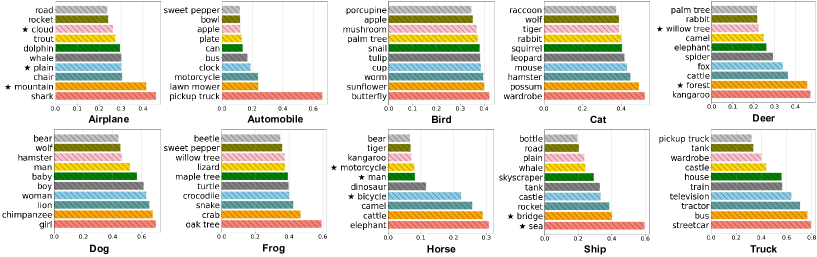
Figure 7: Average top-10 confidences of a CIFAR-10 classifier (WideResNet-40-2) tested on CIFAR-100 (OOD).

In Figure 7, we show additional average softmax probabilities (bars) on OOD samples (row) that are classified as respective CIFAR-10 classes.

B. Visualization of the Surrogate OOD Samples

Figure 8: Qualitative results for inpainting.

We visualize inpainting results at different CAM thresholds $\lambda$ in Figure 8. Key features are incrementally retained with larger thresholds, and we showed that using the threshold of 0.3 generally achieves high OOD detection performance. Additionally, the surrogate OOD images produced by the threshold of 0.3 are qualitatively reasonable.

C. Comparison with Likelihood-based Methods

We also compare with state-of-the-art likelihood-based methods that incorporated generative modeling (Grathwohl et al. 2020; Xiao, Yan, and Amit 2020) (Table 9).

IND Method OOD Datasets SVHN Textures LSUN-crop LSUN-resize Place-365 iSUN FPR AUROC FPR AUROC FPR AUROC FPR AUROC FPR AUROC FPR AUROC $\downarrow$ $\uparrow$ $\downarrow$ $\uparrow$ $\downarrow$ $\uparrow$ $\downarrow$ $\uparrow$ $\downarrow$ $\uparrow$ $\downarrow$ $\uparrow$ CIFAR-10 MSP 48.43 91.91 59.11 88.51 25.52 96.48 53.39 91.07 57.04 89.52 50.11 91.18 $\text{JEM}^{\dagger}$-softmax 80.58 85.25 69.68 87.17 75.05 84.64 62.18 88.42 68.72 85.15 64.69 87.31 JEM-softmax 82.03 83.81 68.88 87.15 81.50 80.67 72.27 85.41 73.91 83.63 72.78 85.05 JEM-likelihood 99.28 52.81 81.70 65.58 99.99 46.75 78.67 66.47 95.38 48.00 74.54 69.52 LR 0.00 97.25 49.99 94.22 66.66 93.32 49.99 94.39 59.99 93.38 66.66 93.01 KIRBY-M 6.31 98.51 21.72 94.87 2.63 99.39 13.13 97.54 26.02 94.34 14.23 97.55 KIRBY-B 4.66 98.99 15.84 95.86 2.05 99.53 5.69 98.66 23.05 95.06 4.96 98.85 CIFAR-100 MSP 84.35 71.37 82.65 73.54 60.33 85.58 83.27 74.11 85.17 70.46 83.24 74.95 $\text{JEM}^{\dagger}$-softmax 73.46 81.55 85.41 70.52 77.84 75.78 86.33 70.61 85.56 67.86 88.64 66.81 JEM-softmax 78.67 78.12 89.61 62.84 90.68 60.32 86.89 67.94 89.29 63.20 88.72 64.64 JEM-likelihood 98.54 51.80 79.06 63.70 99.96 35.70 69.88 76.31 95.57 46.90 66.10 77.11 LR 99.99 91.14 99.99 90.99 66.66 93.06 74.99 93.08 79.99 92.19 83.33 92.49 KIRBY-M 26.71 95.21 38.31 90.91 11.16 97.80 29.02 94.40 70.03 80.70 26.63 94.85 KIRBY-B 14.96 96.26 32.43 91.30 12.50 97.46 14.58 97.24 72.72 78.94 13.03 97.48 STL-10 MSP 95.98 57.56 89.23 64.53 75.59 81.64 77.07 80.91 77.84 80.15 76.57 81.60 $\text{JEM}^{\dagger}$-softmax 87.32 72.96 87.84 68.37 92.38 61.85 90.82 63.80 91.67 62.73 88.27 70.19 JEM-softmax 92.67 69.83 91.90 62.73 92.39 58.62 90.73 64.56 89.19 64.94 83.22 73.38 JEM-likelihood 99.94 57.85 82.89 67.03 95.50 50.55 95.75 57.57 96.56 55.26 98.71 62.23 LR 99.99 27.40 99.99 54.69 99.99 66.13 99.99 72.32 99.99 69.18 99.99 64.81 KIRBY-M 2.41 99.23 65.58 79.22 53.46 89.54 50.49 89.97 53.93 88.47 43.22 90.59 KIRBY-B 1.01 98.90 76.29 69.64 47.16 90.58 43.59 91.30 44.31 90.31 36.36 92.01

Table 9: Comparison with Likelihood-based methods using WideResNet-40-2. $\text{JEM}^{\dagger}$ is trained with WideResNet-28-10.

D. Additional Result

D.1. Comparison with representative methods

WideResNet DenseNet AUROC FPR AUROC FPR CSI (Tack et al. 2020) 92.45 35.66 85.31 47.83 VOS (Du et al. 2022) 94.06 24.87 95.33 22.47 KIRBY-M 97.03 14.01 97.03 14.63 KIRBY-B 97.82 9.37 96.54 15.40

Table 10: OOD detection results with respect to AUROC and FPR, comparing KIRBY with representative methods. All models are trained with CIFAR-10, and we report average AUROC for the six OOD benchmark datasets.

We provide comparison results with KIRBY and additional related works on feature representation learning (Table 10).

D.2. KIRBY Works on Gray-scale Images

In Table 11, we complement our experiments by reporting OOD detection performance on gray-scale pairs with Fashion-MNIST as ID data. We set MNIST (Deng 2012), KMNIST (Clanuwat et al. 2018), and Omniglot (Lake, Salakhutdinov, and Tenenbaum 2015) as OOD, respectively.

Method OOD Datasets MNIST KMNIST Omniglot Average FPR AUROC FPR AUROC FPR AUROC FPR AUROC $\downarrow$ $\uparrow$ $\downarrow$ $\uparrow$ $\downarrow$ $\uparrow$ $\downarrow$ $\uparrow$ MSP 79.00 82.53 69.45 86.61 68.82 89.36 72.43 86.17 ODIN 48.05 91.14 41.44 91.80 43.47 94.06 44.32 92.33 Energy 6.31 98.85 5.89 98.80 2.96 99.32 5.06 98.99 ReAct 4.10 99.22 3.26 99.25 2.03 99.44 3.13 99.30 Mahalanobis 1.71 99.20 0.46 99.64 0.00 99.84 0.72 99.61 DICE 0.63 99.31 0.37 99.68 0.12 99.63 0.37 99.54 LR 98.99 89.26 49.99 94.31 33.33 96.00 61.11 93.19 GAN 53.20 89.57 52.67 89.05 97.95 51.72 67.94 76.78 ACET 3.70 98.65 9.38 98.29 8.72 97.82 7.27 98.25 KIRBY-M 0.13 99.79 0.22 99.88 0.00 99.96 0.12 99.88 KIRBY-B 5.99 98.56 1.91 99.47 0.01 99.99 2.63 99.34

Table 11: Performance on gray-scale data with WideResNet-40-2. JEM suffers from training instability, hence we exclude JEM in this report.

E. Details of Experiments

Training details. We use pre-trained WideResNet-40-2 , ResNet-34 , and DenseNet-BC  for CIFAR-10 and CIFAR-100 experiments. For STL-10, we train classifiers from scratch, and each model is train by minimizing the cross-entropy using SGD with momentum of 0.9. We use the initial learning rate of 0.1 and the learning rate is dropped by a factor of 10 at 50% and 75% of the training progress. Specifically, we train DenseNet-BC for 300 epochs with batch size of 32. ResNet-34 and WideResNet-40-2 are trained for 200 epochs with batch size of 128, respectively.

Software and Hardware. We run all experiments with PyTorch (Paszke et al. 2019) on a single NVIDIA Tesla V100 GPU. In particular, we use Fast Marching inpainting method implemented by OpenCV (Bradski 2000).

References

- Bradski (2000) Bradski, G. 2000. The OpenCV Library. Dr. Dobb’s Journal of Software Tools.
- Cao et al. (2020) Cao, T.; Huang, C.-W.; Hui, D. Y.-T.; and Cohen, J. P. 2020. A benchmark of medical out of distribution detection. arXiv preprint arXiv:2007.04250.
- Chattopadhay et al. (2018) Chattopadhay, A.; Sarkar, A.; Howlader, P.; and Balasubramanian, V. N. 2018. Grad-cam++: Generalized gradient-based visual explanations for deep convolutional networks. In 2018 IEEE winter conference on applications of computer vision (WACV), 839–847. IEEE.
- Cimpoi et al. (2014) Cimpoi, M.; Maji, S.; Kokkinos, I.; Mohamed, S.; and Vedaldi, A. 2014. Describing textures in the wild. In Proceedings of the IEEE conference on computer vision and pattern recognition, 3606–3613.
- Clanuwat et al. (2018) Clanuwat, T.; Bober-Irizar, M.; Kitamoto, A.; Lamb, A.; Yamamoto, K.; and Ha, D. 2018. Deep learning for classical japanese literature. arXiv preprint arXiv:1812.01718.
- Coates, Ng, and Lee (2011) Coates, A.; Ng, A.; and Lee, H. 2011. An analysis of single-layer networks in unsupervised feature learning. In Proceedings of the fourteenth international conference on artificial intelligence and statistics, 215–223. JMLR Workshop and Conference Proceedings.
- Deng (2012) Deng, L. 2012. The mnist database of handwritten digit images for machine learning research. IEEE Signal Processing Magazine, 29(6): 141–142.
- Du et al. (2022) Du, X.; Wang, Z.; Cai, M.; and Li, Y. 2022. VOS: Learning What You Don’t Know by Virtual Outlier Synthesis. Proceedings of the International Conference on Learning Representations.
- Feng, Rosenbaum, and Dietmayer (2018) Feng, D.; Rosenbaum, L.; and Dietmayer, K. 2018. Towards safe autonomous driving: Capture uncertainty in the deep neural network for lidar 3d vehicle detection. In 2018 21st International Conference on Intelligent Transportation Systems (ITSC), 3266–3273. IEEE.
- Filos et al. (2020) Filos, A.; Tigkas, P.; McAllister, R.; Rhinehart, N.; Levine, S.; and Gal, Y. 2020. Can autonomous vehicles identify, recover from, and adapt to distribution shifts? In International Conference on Machine Learning, 3145–3153. PMLR.
- Galerne and Leclaire (2017) Galerne, B.; and Leclaire, A. 2017. Texture inpainting using efficient Gaussian conditional simulation. SIAM Journal on Imaging Sciences, 10(3): 1446–1474.
- Goodfellow et al. (2014) Goodfellow, I.; Pouget-Abadie, J.; Mirza, M.; Xu, B.; Warde-Farley, D.; Ozair, S.; Courville, A.; and Bengio, Y. 2014. Generative adversarial nets. Advances in neural information processing systems, 27.
- Grathwohl et al. (2020) Grathwohl, W.; Wang, K.-C.; Jacobsen, J.-H.; Duvenaud, D.; Norouzi, M.; and Swersky, K. 2020. Your classifier is secretly an energy based model and you should treat it like one. International Conference on Learning Representations.
- He et al. (2016) He, K.; Zhang, X.; Ren, S.; and Sun, J. 2016. Deep residual learning for image recognition. In Proceedings of the IEEE conference on computer vision and pattern recognition, 770–778.
- Hein, Andriushchenko, and Bitterwolf (2019) Hein, M.; Andriushchenko, M.; and Bitterwolf, J. 2019. Why relu networks yield high-confidence predictions far away from the training data and how to mitigate the problem. In Proceedings of the IEEE/CVF Conference on Computer Vision and Pattern Recognition, 41–50.
- Hendrycks and Gimpel (2017) Hendrycks, D.; and Gimpel, K. 2017. A Baseline for Detecting Misclassified and Out-of-Distribution Examples in Neural Networks. Proceedings of International Conference on Learning Representations.
- Hendrycks, Mazeika, and Dietterich (2019) Hendrycks, D.; Mazeika, M.; and Dietterich, T. 2019. Deep Anomaly Detection with Outlier Exposure. Proceedings of the International Conference on Learning Representations.
- Hsu et al. (2020) Hsu, Y. C.; Shen, Y.; Jin, H.; and Kira, Z. 2020. Generalized ODIN: Detecting Out-of-Distribution Image Without Learning From Out-of-Distribution Data. In 2020 IEEE/CVF Conference on Computer Vision and Pattern Recognition (CVPR), 10948–10957.
- Huang et al. (2017) Huang, G.; Liu, Z.; Van Der Maaten, L.; and Weinberger, K. Q. 2017. Densely connected convolutional networks. In Proceedings of the IEEE conference on computer vision and pattern recognition, 4700–4708.
- Ioffe and Szegedy (2015) Ioffe, S.; and Szegedy, C. 2015. Batch normalization: Accelerating deep network training by reducing internal covariate shift. In International conference on machine learning, 448–456. PMLR.
- Jiang et al. (2021) Jiang, P.-T.; Zhang, C.-B.; Hou, Q.; Cheng, M.-M.; and Wei, Y. 2021. LayerCAM: Exploring Hierarchical Class Activation Maps. IEEE Transactions on Image Processing.
- Krizhevsky (2009) Krizhevsky, A. 2009. Learning multiple layers of features from tiny images. Technical report.
- Lake, Salakhutdinov, and Tenenbaum (2015) Lake, B. M.; Salakhutdinov, R.; and Tenenbaum, J. B. 2015. Human-level concept learning through probabilistic program induction. Science, 350(6266): 1332–1338.
- Lee et al. (2018a) Lee, K.; Lee, H.; Lee, K.; and Shin, J. 2018a. Training confidence-calibrated classifiers for detecting out-of-distribution samples. International Conference on Learning Representations.
- Lee et al. (2018b) Lee, K.; Lee, K.; Lee, H.; and Shin, J. 2018b. A simple unified framework for detecting out-of-distribution samples and adversarial attacks. Advances in neural information processing systems, 31.
- Liang, Li, and Srikant (2018) Liang, S.; Li, Y.; and Srikant, R. 2018. Enhancing the reliability of out-of-distribution image detection in neural networks. International Conference on Learning Representations.
- Liu et al. (2020a) Liu, J.; Lin, Z.; Padhy, S.; Tran, D.; Bedrax Weiss, T.; and Lakshminarayanan, B. 2020a. Simple and principled uncertainty estimation with deterministic deep learning via distance awareness. Advances in Neural Information Processing Systems, 33: 7498–7512.
- Liu et al. (2020b) Liu, W.; Wang, X.; Owens, J.; and Li, Y. 2020b. Energy-based out-of-distribution detection. Advances in Neural Information Processing Systems, 33: 21464–21475.
- Ming, Yin, and Li (2022) Ming, Y.; Yin, H.; and Li, Y. 2022. On the impact of spurious correlation for out-of-distribution detection. In Proceedings of the AAAI Conference on Artificial Intelligence, volume 36, 10051–10059.
- Nalisnick et al. (2019) Nalisnick, E.; Matsukawa, A.; Teh, Y. W.; Gorur, D.; and Lakshminarayanan, B. 2019. Do Deep Generative Models Know What They Don’t Know? In International Conference on Learning Representations.
- Nalisnick et al. (2020) Nalisnick, E.; Matsukawa, A.; Teh, Y. W.; and Lakshminarayanan, B. 2020. Detecting Out-of-Distribution Inputs to Deep Generative Models Using Typicality.
- Netzer et al. (2011) Netzer, Y.; Wang, T.; Coates, A.; Bissacco, A.; Wu, B.; and Ng, A. Y. 2011. Reading digits in natural images with unsupervised feature learning.
- Paszke et al. (2019) Paszke, A.; Gross, S.; Massa, F.; Lerer, A.; Bradbury, J.; Chanan, G.; Killeen, T.; Lin, Z.; Gimelshein, N.; Antiga, L.; et al. 2019. Pytorch: An imperative style, high-performance deep learning library. Advances in neural information processing systems, 32: 8026–8037.
- Ren et al. (2019) Ren, J.; Liu, P. J.; Fertig, E.; Snoek, J.; Poplin, R.; Depristo, M.; Dillon, J.; and Lakshminarayanan, B. 2019. Likelihood ratios for out-of-distribution detection. Advances in neural information processing systems, 32.
- Russakovsky et al. (2015) Russakovsky, O.; Deng, J.; Su, H.; Krause, J.; Satheesh, S.; Ma, S.; Huang, Z.; Karpathy, A.; Khosla, A.; Bernstein, M.; et al. 2015. Imagenet large scale visual recognition challenge. International journal of computer vision, 115(3): 211–252.
- Selvaraju et al. (2017) Selvaraju, R. R.; Cogswell, M.; Das, A.; Vedantam, R.; Parikh, D.; and Batra, D. 2017. Grad-cam: Visual explanations from deep networks via gradient-based localization. In Proceedings of the IEEE international conference on computer vision, 618–626.
- Shafaei, Schmidt, and Little (2019) Shafaei, A.; Schmidt, M. W.; and Little, J. 2019. A Less Biased Evaluation of Out-of-distribution Sample Detectors. In BMVC.
- Smilkov et al. (2017) Smilkov, D.; Thorat, N.; Kim, B.; Viégas, F. B.; and Wattenberg, M. 2017. SmoothGrad: removing noise by adding noise. CoRR, abs/1706.03825.
- Sun, Guo, and Li (2021) Sun, Y.; Guo, C.; and Li, Y. 2021. React: Out-of-distribution detection with rectified activations. Advances in Neural Information Processing Systems, 34.
- Sun and Li (2022) Sun, Y.; and Li, Y. 2022. DICE: Leveraging Sparsification for Out-of-Distribution Detection. In European Conference on Computer Vision.
- Tack et al. (2020) Tack, J.; Mo, S.; Jeong, J.; and Shin, J. 2020. CSI: Novelty Detection via Contrastive Learning on Distributionally Shifted Instances. In Advances in Neural Information Processing Systems.
- Telea (2004) Telea, A. 2004. An image inpainting technique based on the fast marching method. Journal of graphics tools, 9(1): 23–34.
- Torralba, Fergus, and Freeman (2008) Torralba, A.; Fergus, R.; and Freeman, W. T. 2008. 80 million tiny images: A large data set for nonparametric object and scene recognition. IEEE transactions on pattern analysis and machine intelligence, 30(11): 1958–1970.
- Van Amersfoort et al. (2020) Van Amersfoort, J.; Smith, L.; Teh, Y. W.; and Gal, Y. 2020. Uncertainty estimation using a single deep deterministic neural network. In International Conference on Machine Learning, 9690–9700. PMLR.
- Van der Maaten and Hinton (2008) Van der Maaten, L.; and Hinton, G. 2008. Visualizing data using t-SNE. Journal of machine learning research, 9(11).
- Xiao, Rasul, and Vollgraf (2017) Xiao, H.; Rasul, K.; and Vollgraf, R. 2017. Fashion-MNIST: a Novel Image Dataset for Benchmarking Machine Learning Algorithms. Cite arxiv:1708.07747Comment: Dataset is freely available at https://github.com/zalandoresearch/fashion-mnist Benchmark is available at http://fashion-mnist.s3-website.eu-central-1.amazonaws.com/.
- Xiao, Yan, and Amit (2020) Xiao, Z.; Yan, Q.; and Amit, Y. 2020. Likelihood regret: An out-of-distribution detection score for variational auto-encoder. Advances in neural information processing systems, 33: 20685–20696.
- Xu et al. (2015) Xu, P.; Ehinger, K. A.; Zhang, Y.; Finkelstein, A.; Kulkarni, S. R.; and Xiao, J. 2015. Turkergaze: Crowdsourcing saliency with webcam based eye tracking. arXiv preprint arXiv:1504.06755.
- Yu et al. (2015) Yu, F.; Seff, A.; Zhang, Y.; Song, S.; Funkhouser, T.; and Xiao, J. 2015. Lsun: Construction of a large-scale image dataset using deep learning with humans in the loop. arXiv preprint arXiv:1506.03365.
- Zagoruyko and Komodakis (2016) Zagoruyko, S.; and Komodakis, N. 2016. Wide Residual Networks. In Richard C. Wilson, E. R. H.; and Smith, W. A. P., eds., Proceedings of the British Machine Vision Conference (BMVC), 87.1–87.12. BMVA Press. ISBN 1-901725-59-6.
- Zhou et al. (2016) Zhou, B.; Khosla, A.; Lapedriza, A.; Oliva, A.; and Torralba, A. 2016. Learning deep features for discriminative localization. In Proceedings of the IEEE conference on computer vision and pattern recognition, 2921–2929.
- Zhou et al. (2017) Zhou, B.; Lapedriza, A.; Khosla, A.; Oliva, A.; and Torralba, A. 2017. Places: A 10 million image database for scene recognition. IEEE transactions on pattern analysis and machine intelligence, 40(6): 1452–1464.