Fast Computation of Optimal Transport via
Entropy-Regularized Extragradient Methods

Abstract

Efficient computation of the optimal transport distance between two distributions serves as an algorithm subroutine that empowers various applications. This paper develops a scalable first-order optimization-based method that computes optimal transport to within $\varepsilon$ additive accuracy with runtime $\widetilde{O}(n^{2}/\varepsilon)$, where $n$ denotes the dimension of the probability distributions of interest. Our algorithm achieves the state-of-the-art computational guarantees among all first-order methods, while exhibiting favorable numerical performance compared to classical algorithms like Sinkhorn and Greenkhorn. Underlying our algorithm designs are two key elements: (a) converting the original problem into a bilinear minimax problem over probability distributions; (b) exploiting the extragradient idea — in conjunction with entropy regularization and adaptive learning rates — to accelerate convergence.

Keywords: optimal transport, extragradient methods, entropy regularization, first-order methods, adaptive learning rates

1 Introduction

Quantifying the distance between two probability distributions is an algorithm subroutine that permeates and empowers a wealth of modern data science applications. For instance, how to measure the difference between the model distribution and the real distribution in generative adversarial networks (Arjovsky et al.,, 2017), how to evaluate the intrinsic dissimilarity between two point clouds in computer graphics (Solomon et al.,, 2015; Kim et al.,, 2013), and how to assess the distribution shift in transfer learning (Gayraud et al.,, 2017), are all representative examples built upon probability distances.

This paper focuses attention on computing an elementary instance within this arena that gains increasing popularity, that is, the optimal transport distance between two distributions (Peyré et al.,, 2019). It also sometimes goes by the name of the earth mover’s distance (Werman et al.,, 1985; Rubner et al.,, 2000; Pele and Werman,, 2009) or the Wasserstein distance (Villani,, 2009). In light of the celebrated Kantorovich relaxation (Kantorovich,, 1942; Peyré et al.,, 2019), computing the optimal transport between two $n$-dimensional probability distributions can be cast as solving a linear program over probability matrices with fixed marginals:

$$\begin{array}[]{cl}\mathop{\text{minimize}}\limits_{\bm{P}\in\mathbb{R}^{n\times n}}&\langle\bm{W},\bm{P}\rangle\\ \text{subject to}&\bm{P}\geq\bm{0},\,\bm{P}\bm{1}=\bm{r},\,\bm{P}^{\top}\bm{1}=\bm{c}.\end{array}$$ (3)

Here, $\bm{r}=[r_{i}]_{1\leq i\leq n}$ and $\bm{c}=[c_{i}]_{1\leq i\leq n}$ are $n$-dimensional probability vectors representing the prescribed row and column marginals, respectively, and $\bm{W}=[w_{i,j}]_{1\leq i,j\leq n}\in\mathbb{R}_{+}^{n\times n}$ stands for a given non-negative cost matrix (so that the objective function $\langle\bm{W},\bm{P}\rangle$ measures the total transportation cost). In a nutshell, the optimal transport problem amounts to finding the most cost-efficient reshaping of one distribution into another, or equivalently, the most economical coupling of the two distributions.

At first glance, the optimal transport problem (3) seems to be readily solvable via relatively mature toolboxes in linear programming. Nevertheless, the unprecedentedly large problem dimensionality in contemporary applications calls for a thorough (re)-examination of existing algorithms, so as to ensure feasibility of computing optimal transport at scale. For example, the linear-programming-based algorithm (Lee and Sidford,, 2014) requires a runtime $\widetilde{O}(n^{2.5})$, which takes much longer than the time needed to read the cost matrix $\bm{W}$. In comparison, another alternative tailored to this problem, called Sinkhorn iteration (Sinkhorn,, 1967; Cuturi,, 2013), exploits the special structure underlying the solution to an entropy-regularized variant of (3). This classical approach and its variants have been shown to be near linear-time (Altschuler et al.,, 2017; Dvurechensky et al.,, 2018; Lin et al.,, 2022), attaining $\varepsilon$ additive accuracy with a computational complexity of $\widetilde{O}(n^{2}/\varepsilon^{2})$. Despite their favorable scaling in $n$, however, the Sinkhorn-type algorithms fall short of achieving optimal scaling in $\varepsilon$, thereby stimulating further pursuit for theoretical improvement. Blanchet et al., (2018); Quanrud, (2018) led this line of studies by developing the first algorithms with theoretical runtime $\widetilde{O}(n^{2}/\varepsilon)$, although practical implementation of these algorithms remain unavailable. Jambulapati et al., (2019) went on to propose an implementable first-order method — i.e., dual extrapolation — that enjoys matching complexity $\widetilde{O}(n^{2}/\varepsilon)$; however, this method is numerically outperformed by Sinkhorn iteration as reported in their experiments. Another recent breakthrough in theoretical computer science van den Brand et al., (2020) solved a more general class of problems called maximum cardinality bipartite matching and showed that even logarithmic $\varepsilon$-dependency is feasible; the lack of practical implementation, once again, inhibits real-world adoption.

In sum, despite an exciting line of theoretical advances towards solving optimal transport, there is significant mismatch between the state-of-the-art theoretical results and the practical runtime. This motivates one to pursue other algorithmic alternatives that could be appealing in both theory and practice.

reference	runtime	algorithm	first-order	implementable?
			method?
Altschuler et al., (2017)	$n^{2}/\varepsilon^{3}$	Sinkhorn	yes	yes
Dvurechensky et al., (2018)	$n^{2}/\varepsilon^{2}$	Sinkhorn	yes	yes
Lin et al., (2022)	$n^{2}/\varepsilon^{2}$	Greenkhorn	yes	yes
Dvurechensky et al., (2018)	$n^{2.5}/\varepsilon$	APDAGD	yes	yes
Lin et al., (2022)
Guminov et al., (2021)	$n^{2.5}/\varepsilon$	AAM	yes	yes
Lin et al., (2022)	$n^{2.5}/\varepsilon$	APDAMD	yes	yes
Chambolle and Contreras, (2022)	$n^{2.5}/\varepsilon$	HPD	yes	yes
Xie et al., 2022a	$n^{2.5}/\varepsilon$	PDASGD	yes	yes
Blanchet et al., (2018)	$n^{2}/\varepsilon$	packing linear program	yes	—
Quanrud, (2018)	$n^{2}/\varepsilon$	packing linear program	yes	—
Blanchet et al., (2018)	$n^{2}/\varepsilon$	matrix scaling	no	—
Lahn et al., (2019)	$n^{2}/\varepsilon+n/\varepsilon^{2}$	combinatorial	no	yes
van den Brand et al., (2020)	$n^{2}\log^{2}(1/\varepsilon)$	max-cardinality	no	—
		bipartite matching
Jambulapati et al., (2019)	$n^{2}/\varepsilon$	dual extrapolation	yes	yes
This work	$n^{2}/\varepsilon$	extragradient	yes	yes

Table 1: Comparisons with prior works. Here, we assume $\|\bm{W}\|_{\infty}=1$ without loss of generality, and we omit all logarithmic factors except for van den Brand et al., (2020) (as its $\varepsilon$-dependency is only logarithmic). In the last column, “—” means that no practical implementation has been available so far.

Main contributions.

In this paper, we contribute to the abovementioned growing literature by proposing a scalable algorithm tailored to the optimal transport problem. Our focal point is first-order optimization-based methods — a family of practically appealing algorithms for large-scale optimization. Our algorithm is built around the following key ideas.

• We start with an $\ell_{1}$-penalized variant of the original problem, and reformulate it into a bilinear minimax problem over two sets of probability distributions.

• In an attempt to solve this minimax problem, we design a variant of entropy-regularized extragradient methods. On a high level, the algorithm performs two mirror-descent-type updates per iteration, with learning rates chosen adaptively in accordance with the corresponding row or column marginals.

Encouragingly, the proposed entropy-regularized extragradient method is capable of achieving $\varepsilon$ additive accuracy with

$$\widetilde{O}\bigg{(}\frac{1}{\varepsilon}\bigg{)}\text{ iterations}\qquad\text{or}\qquad\widetilde{O}\bigg{(}\frac{n^{2}}{\varepsilon}\bigg{)}\text{ runtime},$$ (4)

thus constituting a nearly linear-time algorithm with desired iteration complexity; see Theorem 1. Table 1 provides more detailed comparisons with previous results. In short, our algorithm enjoys computational guarantees that match the best-known theory (i.e., Jambulapati et al., (2019)) among all first-order methods for computing optimal transport, while at the same time compare favorably to the Sinkhorn and Greenkhorn algorithms in numerical experiments.

Notation.

Let $\Delta_{n}\coloneqq\{\bm{x}\in\mathbb{R}^{n}\mid\bm{x}\geq\bm{0},\bm{1}^{\top}\bm{x}=1\}$ and $\Delta_{n\times n}\coloneqq\{\bm{X}\in\mathbb{R}^{n\times n}\mid\bm{1}^{\top}\bm{X}\bm{1}=1,X_{i,j}\geq 0,\forall i,j\}$ denote the $n$-dimensional and $n\times n$-dimensional probability simplices, respectively. For any probability vector $\bm{p}\in\Delta_{d}$, its entropy is defined and denoted by $\mathcal{H}(\bm{p})\coloneqq-\sum_{i=1}^{d}p_{i}\log p_{i}$. For any probability vectors $\bm{p},\bm{q}\in\Delta_{d}$, the Kullback-Leibler (KL) divergence of between $\bm{p}$ and $\bm{q}$ is defined by $\mathsf{KL}(\bm{p}\parallel\bm{q})\coloneqq\sum_{i}p_{i}\log\frac{p_{i}}{q_{i}}$. For any matrix $\bm{W}=[W_{i,j}]_{1\leq i,j\leq n}\in\mathbb{R}^{n\times n}$, we denote by $\|\bm{W}\|_{\infty}\coloneqq\max_{1\leq i,j\leq n}|W_{i,j}|$ its entrywise infinity norm, and $\|\bm{W}\|_{1}\coloneqq\sum_{1\leq i,j\leq n}|W_{i,j}|$ its entrywise $\ell_{1}$ norm. Let $\mathbb{R}^{n\times n}_{+}$ denote the set of all $n\times n$ matrices with non-negative entries. For any matrix $\bm{F}\in\mathbb{R}^{n\times n}_{+}$, let $\mathsf{row}(\bm{F})\coloneqq\bm{F}\bm{1}$ (resp. $\mathsf{col}(\bm{F})\coloneqq\bm{F}^{\top}\bm{1}$) represent an $n$-dimensional vector consisting of all row sums (resp. column sums) of $\bm{F}$, and let $\mathsf{row}_{i}(\bm{F})$ (resp. $\mathsf{col}_{i}(\bm{F})$) denote the sum of the $i$-th row (resp. column) of $\bm{F}$. For any vector $\bm{x}=[x_{i}]_{1\leq i\leq n}\in\mathbb{R}^{n}$, we denote by $\mathsf{diag}(\bm{x})\in\mathbb{R}^{n\times n}$ a diagonal matrix whose diagonals consist of the entries of $\bm{x}$.

2 Algorithm and main results

In this section, we present our algorithm design, followed by its convergence guarantees. Before continuing, let us introduce several more notation that facilitates our discussion. Let $\bm{w}_{i}\in\mathbb{R}^{n}$ represent the $i$-th row of $\bm{W}$; for any $\bm{P}\in\mathbb{R}^{n\times n}_{+}$ obeying $\bm{P}\bm{1}=\bm{r}$, introduce a collection of probability vectors $\{\bm{p}_{i}\in\Delta_{n}\}$ such that $r_{i}\bm{p}_{i}$ represents the $i$-th row of $\bm{P}$; similarly, we denote by $\bm{P}^{\star}$ a solution to the problem (3), and employ $r_{i}\bm{p}_{i}^{\star}$ to represent the $i$-th row of $\bm{P}^{\star}$ (so that $\bm{p}_{i}^{\star}$ is a probability vector). In other words, we can write

$$\bm{W}=\left[\begin{array}[]{c}\bm{w}_{1}^{\top}\\ \bm{w}_{2}^{\top}\\ \vdots\\ \bm{w}_{n}^{\top}\end{array}\right],\qquad\bm{P}=\left[\begin{array}[]{c}r_{1}\bm{p}_{1}^{\top}\\ r_{2}\bm{p}_{2}^{\top}\\ \vdots\\ r_{n}\bm{p}_{n}^{\top}\end{array}\right],\qquad\text{and}\qquad\bm{P}^{\star}=\left[\begin{array}[]{c}r_{1}\bm{p}_{1}^{{}^{\star}\top}\\ r_{2}\bm{p}_{2}^{{}^{\star}\top}\\ \vdots\\ r_{n}\bm{p}_{n}^{{}^{\star}\top}\end{array}\right].$$ (5)

Armed with the above notation, we can readily reformulate (3) as follows

$$\begin{array}[]{cl}\mathop{\text{minimize}}\limits_{\{\bm{p}_{i}\}_{i=1}^{n}}&\sum_{i=1}^{n}r_{i}\langle\bm{w}_{i},\bm{p}_{i}\rangle\\ \text{subject to}&\bm{p}_{i}\in\Delta_{n}~{}(1\leq i\leq n),~{}\sum_{i=1}^{n}r_{i}\bm{p}_{i}=\bm{c},\end{array}$$ (8)

for which $\{\bm{p}_{i}^{\star}\}_{i=1}^{n}$ stands for an optimal solution.

2.1 Approximate transportation solution of a penalized variant

Naturally, the equivalent formulation (8) motivates one to look at a related $\ell_{1}$-penalized problem as follows

$$\mathop{\text{minimize}}\limits_{\{\bm{p}_{i}\in\Delta_{n}\}_{i=1}^{n}}\qquad\frac{1}{2}\sum_{i=1}^{n}r_{i}\langle\bm{w}_{i},\bm{p}_{i}\rangle+\|\bm{W}\|_{\infty}\bigg{\|}\sum_{i=1}^{n}r_{i}\bm{p}_{i}-\bm{c}\bigg{\|}_{1},$$ (9)

a trick that has been adopted in prior optimization literature; see, e.g., Jambulapati et al., (2019). Evidently, if we are able to compute an $\varepsilon$-optimal solution $\{\widehat{\bm{p}}_{i}\}_{i=1}^{n}$ to (9), then one necessarily has

$$\frac{1}{2}\sum_{i=1}^{n}r_{i}\langle\bm{w}_{i},\widehat{\bm{p}}_{i}\rangle \leq\frac{1}{2}\sum_{i=1}^{n}r_{i}\langle\bm{w}_{i},\widehat{\bm{p}}_{i}\rangle+\|\bm{W}\|_{\infty}\bigg{\|}r_{i}\sum_{i=1}^{n}\widehat{\bm{p}}_{i}-\bm{c}\bigg{\|}_{1}\leq\frac{1}{2}\sum_{i=1}^{n}r_{i}\langle\bm{w}_{i},\bm{p}_{i}^{\star}\rangle+\|\bm{W}\|_{\infty}\bigg{\|}r_{i}\sum_{i=1}^{n}\bm{p}^{\star}_{i}-\bm{c}\bigg{\|}_{1}+\varepsilon$$

$$=\frac{1}{2}\sum_{i=1}^{n}r_{i}\langle\bm{w}_{i},\bm{p}_{i}^{\star}\rangle+\varepsilon.$$ (10)

In general, however, the solution to (9) does not satisfy the feasibility constraints of the optimal transport problem, and one still needs to convert it into a feasible transportation plan. This can be accomplished by resorting to the following result derived in Altschuler et al., (2017, Lemma 7).

Lemma 1.

For any non-negative matrix $\widehat{\bm{P}}\in\mathbb{R}^{n\times n}_{+}$, Algorithm 3 (see Appendix A) is able to find a probability matrix $\widetilde{\bm{P}}\in\Delta_{n\times n}$ with $O(n^{2})$ computation complexity such that

$$\widetilde{\bm{P}}\bm{1}=\bm{r},\qquad\widetilde{\bm{P}}^{\top}\bm{1}=\bm{c},\qquad\text{and}\qquad\|\widehat{\bm{P}}-\widetilde{\bm{P}}\|_{1}\leq 2\big{(}\|\widehat{\bm{P}}\bm{1}-\bm{r}\|_{1}+\|\widehat{\bm{P}}^{\top}\bm{1}-\bm{c}\|_{1}\big{)}.$$ (11)

As a consequence, it boils down to finding a near-optimal solution $\{\widehat{\bm{p}}_{i}\}_{1\leq i\leq n}$ to (9) in a computationally efficient manner, while ensuring sufficiently small $\|\sum_{i=1}^{n}r_{i}\widehat{\bm{p}}_{i}-\bm{c}\|_{1}$ (a quantity that is equivalent to $\|\sum_{i=1}^{n}r_{i}\widehat{\bm{p}}_{i}-\bm{c}\|_{1}+\sum_{i=1}^{n}\big{|}r_{i}\widehat{\bm{p}}_{i}^{\top}\bm{1}-r_{i}\big{|}=\|\widehat{\bm{P}}^{\top}\bm{1}-\bm{c}\|_{1}+\|\widehat{\bm{P}}\bm{1}-\bm{r}\|_{1}$ in this case given that $\widehat{\bm{p}}_{i}^{\top}\bm{1}=1$).

2.2 Entropy-regularized extragradient methods

In this subsection, we propose a method for solving the $\ell_{1}$-penalized problem (9). To streamline the presentation, we assume without loss of generality that $\|\bm{W}\|_{\infty}=1$; this can be implemented by running $\bm{W}\leftarrow\bm{W}/\|\bm{W}\|_{\infty}$ at the very beginning of the algorithm.

An equivalent minimax problem and entropy regularization.

The first step of the proposed algorithm lies in converting the objective function of (9) into a bilinear function, for which the key lies in handling the $\ell_{1}$ penalty term. Towards this end, we introduce a set of auxiliary 2-dimensional probability vectors $\bm{\mu}_{j}=[\mu_{j,+},\mu_{j,-}]\in\Delta_{2}$ $(1\leq j\leq n)$. As can be easily verified, this allows us to recast the objective of (9) as follows:

$$\frac{1}{2}\sum_{i=1}^{n}r_{i}\langle\bm{w}_{i},\bm{p}_{i}\rangle+\bigg{\|}\sum_{i=1}^{n}r_{i}\bm{p}_{i}-\bm{c}\bigg{\|}_{1}=\max_{\bm{\mu}_{j}\in\Delta_{2},\forall j}f\big{(}\{\bm{p}_{i}\}_{i=1}^{n},\{\bm{\mu}_{j}\}_{j=1}^{n}\big{)},$$ (12)

where we define

$$f\big{(}\{\bm{p}_{i}\}_{i=1}^{n},\{\bm{\mu}_{j}\}_{j=1}^{n}\big{)} \coloneqq\frac{1}{2}\sum_{i=1}^{n}r_{i}\langle\bm{w}_{i},\bm{p}_{i}\rangle+\sum_{j=1}^{n}\big{(}\mu_{j,+}-\mu_{j,-}\big{)}\bigg{(}\sum_{i=1}^{n}r_{i}p_{i,j}-c_{j}\bigg{)}$$

$$=\frac{1}{2}\sum_{i=1}^{n}r_{i}\langle\bm{w}_{i},\bm{p}_{i}\rangle-\sum_{j=1}^{n}(\mu_{j,+}-\mu_{j,-})c_{j}+\sum_{i=1}^{n}\sum_{j=1}^{n}r_{i}(\mu_{j,+}-\mu_{j,-})p_{i,j}.$$ (13)

Armed with this function, one can readily recast (9) as the following minimax problem:

$$\mathop{\text{minimize}}_{\bm{p}_{i}\in\Delta_{n},\forall i}~{}\max_{\bm{\mu}_{j}\in\Delta_{2},\forall j}f\big{(}\{\bm{p}_{i}\}_{i=1}^{n},\{\bm{\mu}_{j}\}_{j=1}^{n}\big{)},$$ (14)

or equivalently (by virtue of von Neumann’s minimax theorem (von Neumann,, 1928)),

$$\mathop{\text{maximize}}_{\bm{\mu}_{j}\in\Delta_{2},\forall j}\min_{\bm{p}_{i}\in\Delta_{n},\forall i}f\big{(}\{\bm{p}_{i}\}_{i=1}^{n},\{\bm{\mu}_{j}\}_{j=1}^{n}\big{)}.$$ (15)

Given that the bilinear objective function is convex-concave but not strongly-convex-strongly-concave, one strategy for accelerating the optimization procedure is to augment the objective function with entropy regularization terms. This leads to the following entropy-regularized minimax problem:

$$\mathop{\text{maximize}}_{\bm{\mu}_{j}\in\Delta_{2},\forall j}\min_{\bm{p}_{i}\in\Delta_{n},\forall i}F\big{(}\{\bm{p}_{i}\}_{i=1}^{n},\{\bm{\mu}_{j}\}_{j=1}^{n}\big{)}\coloneqq f\big{(}\{\bm{p}_{i}\}_{i=1}^{n},\{\bm{\mu}_{j}\}_{j=1}^{n}\big{)}+\sum_{j=1}^{n}\tau_{\mu,j}\mathcal{H}(\bm{\mu}_{j})-\sum_{i=1}^{n}\tau_{p,i}\mathcal{H}(\bm{p}_{i}),$$ (16)

where $\mathcal{H}(\cdot)$ denotes the entropy (which is a strongly concave and non-negative function), and $\{\tau_{\mu,j}\}_{1\leq j\leq n}$ and $\{\tau_{p,i}\}_{1\leq i\leq n}$ are a set of positive regularization parameters that we shall specify momentarily. The remainder of this subsection is dedicated to solving (16) in an efficient fashion.

An extragradient method for solving (16).

The family of extragradient methods has proven effective for solving convex-concave minimax problems (Korpelevich,, 1976; Tseng,, 1995; Harker and Pang,, 1990; Mokhtari et al., 2020a, ). Inspired by a recent development Cen et al., (2021), we propose to solve (16) by means of a variant of extragradient methods.

Let us begin by introducing a basic operation. Suppose the current iterate is $\big{(}\{\bm{p}_{i}^{\mathsf{current}}\}_{i=1}^{n},\{\bm{\mu}_{j}^{\mathsf{current}}\}_{j=1}^{n}\big{)}$. One step of mirror descent (with the KL divergence chosen to monitor the displacement) takes the following form:

$$\bm{\mu}_{j}^{\mathsf{next}} =\arg\max_{\bm{\mu}_{j}\in\Delta_{2}}\left\{\Big{\langle}\nabla_{\bm{\mu}_{j}}F\big{(}\{\bm{p}_{i}^{\mathsf{grad}}\}_{i=1}^{n},\{\bm{\mu}_{j}^{\mathsf{grad}}\}_{j=1}^{n}\big{)},\,\bm{\mu}_{j}\Big{\rangle}-\frac{1}{\eta_{\mu,j}}\mathsf{KL}\big{(}\bm{\mu}_{j}\parallel\bm{\mu}_{j}^{\mathsf{current}}\big{)}\right\}, 1\leq j\leq n$$ (17a)

$$\bm{p}_{i}^{\mathsf{next}} =\arg\min_{\bm{p}_{i}\in\Delta_{n}}\left\{\Big{\langle}\nabla_{\bm{p}_{i}}F\big{(}\{\bm{p}_{i}^{\mathsf{grad}}\}_{i=1}^{n},\{\bm{\mu}_{j}^{\mathsf{grad}}\}_{j=1}^{n}\big{)},\,\bm{p}_{i}\Big{\rangle}+\frac{1}{\eta_{p,i}}\mathsf{KL}\big{(}\bm{p}_{i}\parallel\bm{p}_{i}^{\mathsf{current}}\big{)}\right\}, 1\leq i\leq n$$ (17b)

or equivalently,

$$\mu_{j,s}^{\mathsf{next}} \propto\big{(}\mu_{j,s}^{\mathsf{current}}\big{)}^{1-\eta}\exp\bigg{(}\eta_{\mu,j}s\Big{(}\sum_{i=1}^{n}r_{i}p_{i,j}^{\mathsf{grad}}-c_{j}\Big{)}\bigg{)},\qquad s\in\{+,-\}$$ (18a)

$$p_{i,l}^{\mathsf{next}} \propto\big{(}p_{i,l}^{\mathsf{current}}\big{)}^{1-\eta}\exp\Big{(}-\eta_{p,i}r_{i}\big{(}0.5w_{i,l}+\mu_{l,+}^{\mathsf{grad}}-\mu_{l,-}^{\mathsf{grad}}\big{)}\Big{)},\qquad l=1,\cdots,n$$ (18b)

for all $1\leq i,j\leq n$, where $\{\eta_{\mu,j}\}$ and $\{\eta_{p,i}\}$ are two collections of positive learning rates. Here, we allow the gradient $\nabla F$ to be evaluated at a point $\big{(}\{\bm{p}_{i}^{\mathsf{grad}}\}_{i=1}^{n},\{\bm{\mu}_{j}^{\mathsf{grad}}\}_{j=1}^{n}\big{)}$ deviating from the current iterate $\big{(}\{\bm{p}_{i}^{\mathsf{current}}\}_{i=1}^{n},\{\bm{\mu}_{j}^{\mathsf{current}}\}_{j=1}^{n}\big{)}$, which plays a crucial role in describing the extragradient update rule.

We are now ready to present the proposed method, which maintains several sequences of the iterates; for each iteration $t$, we maintain and update the following iterates:

• Updates w.r.t. the variables $\{\bm{p}_{i}\}_{i=1}^{n}$: main sequence $\{\bm{p}_{i}^{t}\in\Delta_{n}\}_{i=1}^{n}$; midpoints $\{\overline{\bm{p}}_{i}^{t}\in\Delta_{n}\}_{i=1}^{n}$.

• Updates w.r.t. the variables $\{\bm{\mu}_{j}\}_{j=1}^{n}$: main sequence $\{\bm{\mu}_{j}^{t}=[\mu_{j,+}^{t},\mu_{j,-}^{t}]\in\Delta_{2}\}_{j=1}^{n}$; midpoints $\{\overline{\bm{\mu}}_{j}^{t}=[\overline{\mu}_{j,+}^{t},\overline{\mu}_{j,-}^{t}]\in\Delta_{2}\}_{j=1}^{n}$; adjusted main sequence $\{\bm{\mu}_{j}^{t,\mathsf{adjust}}=[\mu_{j,+}^{t,\mathsf{adjust}},\mu_{j,-}^{t,\mathsf{adjust}}]\in\Delta_{2}\}_{j=1}^{n}$.

In the $t$-th iteration, the proposed algorithm performs the following three sets of updates, with the first two embodying the extragradient idea.

• Computing the midpoints: for each $1\leq j\leq n$,

  $$\overline{\mu}_{j,s}^{t+1}\propto\big{(}\mu_{j,s}^{t,\mathsf{adjust}}\big{)}^{1-\eta}\exp\bigg{(}\eta_{\mu,j}s\Big{(}\sum_{i=1}^{n}r_{i}p_{i,j}^{t}-c_{j}\Big{)}\bigg{)},\qquad s\in\{+,-\},$$ (19a)

  and for each $$1\leq i\leq n$$,

  $$\overline{p}_{i,j}^{t+1}\propto\big{(}p_{i,j}^{t}\big{)}^{1-\eta}\exp\Big{(}-\eta_{p,i}r_{i}\big{(}0.5w_{i,j}+\mu_{j,+}^{t,\mathsf{adjust}}-\mu_{j,-}^{t,\mathsf{adjust}}\big{)}\Big{)},\qquad j=1,\cdots,n,$$ (19b)

  with the learning rates $$\{\eta_{\mu,j}\} \{\eta_{p,i}\} \big{(}\{\bm{p}_{i}^{t}\}_{i=1}^{n},\{\bm{\mu}_{j}^{t,\mathsf{adjust}}\}_{j=1}^{n}\big{)}$$ and to be specified shortly. In words, this constitutes one step of mirror descent (cf. (18)) from the point , with the gradient evaluated at the same point.

• Updating the main sequence: for each $1\leq j\leq n$,

  $$\mu_{j,s}^{t+1}\propto\big{(}\mu_{j,s}^{t,\mathsf{adjust}}\big{)}^{1-\eta}\exp\bigg{(}\eta_{\mu,j}s\Big{(}\sum_{i=1}^{n}r_{i}\overline{p}_{i,j}^{t+1}-c_{j}\Big{)}\bigg{)},\qquad s\in\{+,-\};$$ (20a)

  and for each $$1\leq i\leq n$$,

  $$p_{i,j}^{t+1}\propto\big{(}p_{i,j}^{t}\big{)}^{1-\eta}\exp\Big{(}-\eta_{p,i}r_{i}\big{(}0.5w_{i,j}+\overline{\mu}_{j,+}^{t+1}-\overline{\mu}_{j,-}^{t+1}\big{)}\Big{)},\qquad j=1,\cdots,n.$$ (20b)

  This implements another step of mirror descent (cf. (18)) from the same point $$\big{(}\{\bm{p}_{i}^{t}\}_{i=1}^{n},\{\bm{\mu}_{j}^{t,\mathsf{adjust}}\}_{j=1}^{n}\big{)} \big{(}\{\overline{\bm{p}}_{i}^{t+1}\}_{i=1}^{n},\{\overline{\bm{\mu}}_{j}^{t+1}\}_{j=1}^{n}\big{)}$$ as above, albeit using a gradient evaluated at the midpoint . In a nutshell, the midpoint computed in the previous step assists in predicting a better search direction.

• Adjusting the current iterates: for each $1\leq j\leq n$,

  $$\mu_{j,s}^{t+1,\mathsf{adjust}}\propto\max\Big{\{}\mu_{j,s}^{t+1},\,e^{-B}\max\big{\{}\mu_{j,+}^{t+1},\mu_{j,-}^{t+1}\big{\}}\Big{\}},\qquad s\in\{+,-\},$$ (20c)

  where $B>0$ is some parameter to be specified momentarily. This operation prevents the ratio $\frac{\max\{\mu_{j,+}^{t+1},\mu_{j,-}^{t+1}\}}{\min\{\mu_{j,+}^{t+1},\mu_{j,-}^{t+1}\}}$ from being exponentially large (i.e., it is no larger than $e^{B}$), a condition that helps facilitate analysis.

After running the above updates for $t_{\max}$ iterations, we reach a probability matrix taking the following form:

$$\widehat{\bm{P}}=\big{[}r_{1}\bm{p}_{1}^{t_{\max}},\ldots,r_{n}\bm{p}_{n}^{t_{\max}}\big{]}^{\top},$$ (21)

which can be converted into a feasible transportation plan $\widetilde{\bm{P}}$ by invoking Algorithm 3. The whole procedure is summarized in Algorithm 1.

1 Input: cost matrix $\bm{W}\in\mathbb{R}_{+}^{n\times n}$, probability vectors $\bm{r}=[r_{i}]_{1\leq i\leq n},\bm{c}=[c_{i}]_{1\leq i\leq n}\in\Delta_{n}$, target accuracy level $\varepsilon$, number of iterations $t_{\max}$.

2

// Initialization

3 $\mu_{j,+}^{0}=\mu_{j,-}^{0}=\mu_{j,+}^{0,\mathsf{adjust}}=\mu_{j,-}^{0,\mathsf{adjust}}=1/2$ for all $1\leq j\leq n$; $\bm{p}_{i}^{0}=[1/n,\ldots,1/n]$ for all $1\leq i\leq n$.

$\bm{W}\leftarrow\bm{W}/\|\bm{W}\|_{\infty}$; $\varepsilon\leftarrow\varepsilon/\|\bm{W}\|_{\infty}$. /* normalization */

4

// Main loop

5 for $t=0$ to $t_{\max}-1$ do

       // Compute the midpoints

6       for $j=1$ to $n$ do

7             $\overline{\mu}_{j,s}^{t+1}\leftarrow\big{(}\mu_{j,s}^{t,\mathsf{adjust}}\big{)}^{1-\eta}\exp\Big{(}\eta_{\mu,j}s\big{(}\sum_{i=1}^{n}r_{i}p_{i,j}^{t}-c_{j}\big{)}\Big{)},\qquad\hfill s\in\{+,-\};$

             $\overline{\bm{\mu}}_{j}^{t+1}\leftarrow\mathtt{Normalize}(\overline{\bm{\mu}}_{j}^{t+1})$. /* Call Algorithm 2 */

8            

9      for $i=1$ to $n$ do

10             $\overline{p}_{i,j}^{t+1}\leftarrow\big{(}p_{i,j}^{t}\big{)}^{1-\eta}\exp\Big{(}-\eta_{p,i}r_{i}\big{(}0.5w_{i,j}+\mu_{j,+}^{t,\mathsf{adjust}}-\mu_{j,-}^{t,\mathsf{adjust}}\big{)}\Big{)},\qquad\hfill j=1,\cdots,n$;

             $\overline{\bm{p}}_{i}^{t+1}\leftarrow\mathtt{Normalize}(\overline{\bm{p}}_{i}^{t+1})$. /* Call Algorithm 2 */

11            

12      

      // Update the main sequence

13       for $j=1$ to $n$ do

14             $\mu_{j,s}^{t+1}\leftarrow\big{(}\mu_{j,s}^{t,\mathsf{adjust}}\big{)}^{1-\eta}\exp\bigg{(}\eta_{\mu,j}s\Big{(}\sum_{i=1}^{n}r_{i}\overline{p}_{i,j}^{t+1}-c_{j}\Big{)}\bigg{)},\qquad\hfill s\in\{+,-\}$;

             $\bm{\mu}_{j}^{t+1}\leftarrow\mathtt{Normalize}(\bm{\mu}_{j}^{t+1})$. /* Call Algorithm 2 */

15            

16      for $i=1$ to $n$ do

17             $p_{i,j}^{t+1}\leftarrow\big{(}p_{i,j}^{t}\big{)}^{1-\eta}\exp\Big{(}-\eta_{p,i}r_{i}\big{(}0.5w_{i,j}+\overline{\mu}_{j,+}^{t+1}-\overline{\mu}_{j,-}^{t+1}\big{)}\Big{)},\qquad\hfill j=1,\cdots,n$;

             $\bm{p}_{i}^{t+1}\leftarrow\mathtt{Normalize}(\bm{p}_{i}^{t+1})$. /* Call Algorithm 2 */

18            

19      

      // Adjust the main sequence

20       for $j=1$ to $n$ do

21             $\mu_{j,s}^{t+1,\mathsf{adjust}}\leftarrow\max\big{\{}\mu_{j,s}^{t+1},\,e^{-B}\max\big{\{}\mu_{j,+}^{t+1},\mu_{j,-}^{t+1}\big{\}}\big{\}},\qquad\hfill s\in\{+,-\}$;

             $\bm{\mu}_{j}^{t+1,\mathsf{adjust}}\leftarrow\mathtt{Normalize}(\bm{\mu}_{j}^{t+1,\mathsf{adjust}})$. /* Call Algorithm 2 */

22            

23      

24

Set $\widehat{\bm{P}}=[r_{1}\bm{p}_{1}^{t_{\max}},\ldots,r_{n}\bm{p}_{n}^{t_{\max}}]^{\top}$. /* Solution of regularized problem (9) */

// Convert an almost-transportation plan $\widehat{\bm{P}}$ to a feasible transportation plan $\widetilde{\bm{P}}$

25

26Output $\widetilde{\bm{P}}$, obtained by invoking Algorithm 3 with input $\widehat{\bm{P}}$.

Algorithm 1 The proposed entropy-regularized extragradient method for optimal transport.

1

2Input: $\bm{x}=[x_{i}]_{1\leq i\leq d}$

3Output $\bm{y}=[y_{i}]_{1\leq i\leq d}$, where $y_{i}=\frac{x_{i}}{\sum_{j}x_{j}}$.

Algorithm 2 $\mathtt{Normalize}(\bm{x})$.

Choice of algorithmic parameters.

Thus far, we have not yet discussed the choices of multiple parameters required to run Algorithm 1. Let us begin by looking at the regularization parameters $\{\tau_{\mu,j}\}$ and $\{\tau_{p,j}\}$, which cannot be taken to be too large. Evidently, if the regularization parameters are chosen such that

$$\sum_{j=1}^{n}\tau_{\mu,j}\log 2+\sum_{i=1}^{n}\tau_{p,i}\log n\leq\varepsilon,$$ (22)

then it follows from elementary properties of the entropy that: for any $\{\bm{p}_{i}\in\Delta_{n}\}_{i=1}^{n}$ and $\{\bm{\mu}_{j}\in\Delta_{2}\}_{i=1}^{n}$,

$$\Big{|}F\big{(}\{\bm{p}_{i}\}_{i=1}^{n},\{\bm{\mu}_{j}\}_{i=1}^{n}\big{)}-f\big{(}\{\bm{p}_{i}\}_{i=1}^{n},\{\bm{\mu}_{j}\}_{i=1}^{n}\big{)}\Big{|}\leq\sum_{j=1}^{n}\tau_{\mu,j}\log 2+\sum_{i=1}^{n}\tau_{p,i}\log n\leq\varepsilon.$$ (23)

Consequently, any $\varepsilon$-optimal solution to (16) is an $2\varepsilon$-optimal solution to (9). Moverover, the theory developed in Cen et al., (2021) for matrix games suggests that a feasible learning rate can be chosen to be inversely proportional to the regularization parameter. As a result, we take

$$\eta_{\mu,j}=\frac{\eta}{\tau_{\mu,j}}\qquad\text{and}\qquad\eta_{p,i}=\frac{\eta}{\tau_{p,i}},\qquad\forall 1\leq i,j\leq n$$ (24)

for some quantity $\eta>0$.

With the above considerations in mind, we recommend the following choices of parameters:

$$B=C_{1}\log\frac{n}{\varepsilon},\qquad\eta=\frac{C_{2}^{2}\varepsilon}{\sqrt{B}\log n},\qquad\eta_{\mu,j}=\frac{15C_{2}\sqrt{B}}{c_{j}+C_{3}/n},\qquad\eta_{p,i}=\frac{C_{2}}{\sqrt{B}r_{i}},\qquad\forall 1\leq i,j\leq n$$ (25)

with $C_{1}>0,C_{2}>0,0<C_{3}\leq 1$ some suitable universal constants, which correspond to

$$\tau_{\mu,j}=\frac{\eta}{\eta_{\mu,j}}=\frac{C_{2}(c_{j}+C_{3}/n)\varepsilon}{15C_{1}(\log n)\big{(}\log\frac{n}{\varepsilon}\big{)}}\qquad\text{and}\qquad\tau_{p,i}=\frac{\eta}{\eta_{p,i}}=\frac{C_{2}r_{i}\varepsilon}{\log n},\qquad\forall 1\leq i,j\leq n.$$ (26)

Three remarks are in order. Firstly, the learning rate $\eta_{p,i}$ (resp. $\eta_{\mu,j}$) is chosen adaptively to be inversely proportional to the row sum $r_{i}$ (resp. column sum $c_{j}$), which is crucial in achieving our advertised convergence rate; in contrast, fixing the learing rates across all $i$ (resp. $j$) as in prior works results in slow convergence particularly when the $r_{i}$’s (resp. $c_{j}$’s) are far from uniform. Secondly, $\eta_{\mu,j}(c_{j}+O(1/n))$ is chosen to be larger than $\eta_{p,i}r_{i}$, in the hope that $\{\bm{\mu}_{j}^{t}\}$ converges more rapidly than $\{\bm{p}_{i}^{t}\}$. Furthermore, if $C_{1}$ is large enough and $C_{2}$ small enough, the above regularization parameters obey

$$\sum_{j=1}^{n}\tau_{\mu,j}\log 2+\sum_{i=1}^{n}\tau_{p,i}\log n=\frac{C_{2}(1+C_{3})\varepsilon\log 2}{15C_{1}\log n\log\frac{n}{\varepsilon}}+C_{2}\varepsilon\leq\varepsilon$$ (27)

given that $\sum_{j}c_{j}=\sum_{i}r_{i}=1$, thus satisfying (23).

2.3 Theoretical guarantees

Our theoretical analysis delivers intriguing news about the convergence properties of the proposed algorithm, as asserted by the following theorem.

Theorem 1.

Consider any $0<\varepsilon<\|\bm{W}\|_{\infty}$. Algorithm 1 with the parameters (25) returns a probability matrix $\widetilde{\bm{P}}\in\Delta_{n\times n}$ obeying

$$\widetilde{\bm{P}}\bm{1}=\bm{r},\qquad\widetilde{\bm{P}}^{\top}\bm{1}=\bm{c},\qquad\text{and}\qquad\langle\bm{W},\widetilde{\bm{P}}\rangle\leq\langle\bm{W},\bm{P}^{\star}\rangle+\varepsilon,$$ (28)

provided that $C_{1}>0$ is large enough, $C_{2}>0$ is small enough, $C_{2}\sqrt{C_{1}}$ is large enough, $0<C_{3}\leq 1$, $C_{2}^{2}/C_{3}$ is small enough, and

$$t_{\max}\geq C_{4}\frac{\|\bm{W}\|_{\infty}}{\eta}\log\Big{(}\frac{n\|\bm{W}\|_{\infty}}{\varepsilon}\Big{)}$$ (29)

for some large enough constant $C_{4}>0$, with $\eta$ defined in (25).

Assuming without loss of generality that $\|\bm{W}\|_{\infty}=1$, Theorem 1 in conjunction with the choice of $\eta$ in (25) asserts that the iteration complexity of our algorithm is

$$\text{(iteration complexity)}\qquad O\bigg{(}\frac{1}{\varepsilon}\log^{2.5}\frac{n}{\varepsilon}\bigg{)}.$$ (30)

Given that each iteration can be implemented in $O(n^{2})$ time, the total computational complexity of Algorithm 1 is no larger than

$$\text{(computation complexity)}\qquad O\bigg{(}\frac{n^{2}}{\varepsilon}\log^{2.5}\frac{n}{\varepsilon}\bigg{)}.$$ (31)

This matches the state-of-the-art theory Jambulapati et al., (2019) among all first-order methods tailored to the optimal transport problem; we shall demonstrate the practical efficacy of our algorithm momentarily. In comparison to Blanchet et al., (2018); Quanrud, (2018); van den Brand et al., (2020), our algorithm is easy-to-implement and amenable to parallelism, without the need of calling any unimplementable blackbox subroutine that is still only of theoretical interest.

Finally, we note that while our analysis is inspired by the prior work Cen et al., (2021), a direct application of their analysis framework can only lead to highly suboptimal iteration complexity. Particularly, they focus on the $\ell_{\infty}$ type bound, which can ensure $\|\widehat{\bm{P}}^{\top}\bm{1}-\bm{c}\|_{\infty}\leq\varepsilon$ within $\widetilde{O}\big{(}\frac{1}{\varepsilon}\big{)}$ iterations. However, we need $\|\widehat{\bm{P}}^{\top}\bm{1}-\bm{c}\|_{1}\leq\varepsilon$ when paired with Lemma 1 to get our desired result, which in turn requires $\widetilde{O}\big{(}\frac{n^{3}}{\varepsilon}\big{)}$ computation complexity if naively adopting the $\ell_{\infty}$ type bound in Cen et al., (2021). Novel algorithmic and analysis ideas (e.g., how to exploit the use of adaptive learning rates) tailored to the optimal transport problem play a central role in establishing the desired performance guarantees.

3 Related works

In this section, we discuss a broader set of past works that are related to this paper.

Entropy regularization.

The advantages of entropy regularization have been exploited in a diverse array of optimization problems over probability distributions, with prominent examples including equilibrium computation in game theory (Ao et al.,, 2023; McKelvey and Palfrey,, 1995; Savas et al.,, 2019; Mertikopoulos and Sandholm,, 2016; Cen et al.,, 2021; Cen et al., 2022a, ) and policy optimization in reinforcement learning (Geist et al.,, 2019; Neu et al.,, 2017; Mei et al.,, 2020; Cen et al.,, 2023; Cen et al., 2022b, ; Lan,, 2022; Zhan et al.,, 2023). The idea of employing entropy regularization to speed up convergence in optimal transport has been studied for multiple decades (e.g., Knight, (2008); Kalantari et al., (2008); Chakrabarty and Khanna, (2021); Altschuler, (2022)) and recently popularized by Cuturi, (2013). By adding a reasonably small entropy penalty term (so that it does not bias the objective function by much), the optimal solution to the entropy-regularized problem exhibits a special form $\bm{D}_{r}\exp(-\eta\bm{W})\bm{D}_{c}$, where $\bm{D}_{r}$ and $\bm{D}_{c}$ are certain diagonal matrices and the $\exp(\cdot)$ operator is applied in an entrywise manner (Sinkhorn,, 1967). This special structure motivates one to alternate between row and column rescaling until convergence, the key idea behind the Sinkhorn algorithm.

Extragradient methods.

Dating back to Korpelevich, (1976); Tseng, (1995), extensive research efforts have been put forth towards understanding extragradient methods for saddle-point optimization, where a clever step of extrapolation is leveraged to accelerate convergence; partial examples include the optimistic gradient descent ascent (OGDA) method (Mertikopoulos et al., 2018b, ; Mertikopoulos et al., 2018a, ; Rakhlin and Sridharan,, 2013; Wei et al.,, 2021), the implicit update method (Liang and Stokes,, 2019), and their stochastic variants (Hsieh et al.,, 2019). Mokhtari et al., 2020b analyzed the convergence of extragradient methods for unconstrained smooth convex-concave saddle-point problems under the Euclidean metric, with Wei et al., (2021) focusing on constrained saddle-point problems. While earlier works analyzed primarily average-iterate or ergodic convergence (Nemirovski,, 2004), significant emphasis was put on achieving last-iterate convergence motivated by machine learning applications (Mertikopoulos et al., 2018b, ; Wei et al.,, 2021). By using entropy regularization, Cen et al., (2021) demonstrated fast last-iterate convergence of extragradient methods for matrix games, under weaker assumptions than those needed for solving the unregularized games directly (Daskalakis and Panageas,, 2018).

Prior algorithms for the optimal transport problem.

Earlier effort towards computing the optimal transport include the development of the Hungarian algorithm, which is not a linear-time algorithm due to its complexity $\widetilde{O}(n^{3})$ (Kuhn,, 1956; Munkres,, 1957); this algorithm has recently been revisited by Xie et al., 2022b , which further came up with a variant that runs faster in a special class of problem instances. In comparison, Sinkhorn iteration and its variants have achieved widespread adoption in practice since Cuturi, (2013). Altschuler et al., (2017) developed the first theory uncovering the linear-time feature of Sinkhorn iteration with computational complexity $\widetilde{O}(n^{2}/\varepsilon^{3})$, and inspired a recent strand of works (e.g., Dvurechensky et al., (2018); Feydy et al., (2019)) that strengthened the runtime for Sinkhorn-type algorithms to $\widetilde{O}(n^{2}/\varepsilon^{2})$ (including a fast greedy variant called the Greenkhorn algorithm (Altschuler et al.,, 2017; Lin et al.,, 2022)). First-order methods algorithms and their stochastic variants have received much recent attention, including but not limited to accelerated gradient descent (Dvurechensky et al.,, 2018), stochastic gradient descent (SGD) (Genevay et al.,, 2016), and accelerated primal-dual methods (Lin et al.,, 2022; Xie et al., 2022a, ; Chambolle and Contreras,, 2022). The convergence guarantees of these algorithms remain suboptimal in terms of the dependency on either $n$ or $\varepsilon$.

As mentioned previously, the algorithms designed by Blanchet et al., (2018); Quanrud, (2018), while achieving an appealing $\widetilde{O}(n^{2}/\varepsilon)$ runtime, rely heavily on reduction to blackbox methods developed in theoretical computer science (e.g., positive linear programming (Allen-Zhu and Orecchia,, 2015)), which hinder practical realization and do not yet admit fast parallelization. Inspired by Nesterov, (2007); Sherman, (2017), Jambulapati et al., (2019) leveraged the concept of area convexity when designing and analyzing the dual extrapolation algorithm, which has become the best-performing (in theory) first-order method in the previous literature. It is also worth noting that Jambulapati et al., (2019) also reformulated the problem into a minimax form, albeit using different constraint sets (for instance, the decision variables therein are not all probability vectors). Finally, another recent work Lahn et al., (2019) tackled this problem via combinatorial algorithms, yielding a runtime as fast as $\widetilde{O}(n^{2}/\varepsilon+n/\varepsilon^{2})$.

4 Numerical experiments

To demonstrate the practical applicability of the proposed algorithm, we compare its empirical performance with that of the Sinkhorn algorithm and its greedy variant called Greenkhorn, which are still among the most widely used baselines for solving optimal transport.

Setup.

Our experimental setup is similar to the ones adopted in Altschuler et al., (2017); Jambulapati et al., (2019); Lin et al., (2022). To generate an optimal transport problem instance, we first produce two $m\times m$ images in one of the following ways.

• “Synthetic”: each image has a randomly placed square foreground that accounts for $50\%$ of the pixels; the foreground and background have pixel values uniformly sampled from $[0,10]$ and $[0,1]$, respectively.

• “MNIST”: a pair of images are randomly selected from the MNIST dataset, and downsampled to size $m\times m$; then, a value of $0.01$ is added to all pixels.

With two $m\times m$ images in place, we flatten and normalize them to obtain $\bm{r},\bm{c}\in^{n}$, where $n=m^{2}$. In addition, we let each entry of the cost matrix $\bm{W}\in^{n\times n}$ be the $\ell_{1}$ distance between each pair of pixels in an $m\times m$ image. For each optimal transport instance, we also assign a target accuracy level $\varepsilon$, which will be employed to set parameters of the algorithms.

Each algorithm is implemented with varying parameters. For the Sinkhorn and Greenkhorn algorithms, recall from Altschuler et al., (2017) that $\eta^{-1}$ is the strength of entropic regularization; in our experiments, we consider the theoretical choice $\eta=4\varepsilon^{-1}\log n$, as well as less conservative options $\eta\in\{10,100,500\}$. Regarding the proposed extragradient method, recall that Algorithm 1 requires parameters $B,\eta,\{\eta_{p,i}\},\{\eta_{\mu,j}\}$. We let $\eta_{p,i}=C/(\sqrt{B}r_{i}),\eta_{\mu,j}=C\sqrt{B}/(c_{j}+C_{3}/n)$, and consider two options: (1) the theoretical choice according to (25), with $B=\log(n/\varepsilon),\eta=\varepsilon/(\sqrt{B}\log n)$ and $C=1,C_{3}=1$; (2) a fine-tuned option, with $B=1,\eta=0,C=1,C_{3}=10^{-2}$.

Numerical comparisons.

The numerical results for various settings are illustrated in Figure 1. Each subfigure represents one randomly generated problem instance. The $X$-axis reflects the computation cost, measured by the total number of matrix-vector products (akin to Jambulapati et al., (2019)); the $Y$-axis reports the gap between the cost of the current iterate (rounded to the probability simplex with marginals $\bm{r}$ and $\bm{c}$) and the true optimal transport value (computed via standard linear programming). The curves w.r.t. Sinkhorn, Greenkhorn and the extragradient method are plotted in blue, green and red, respectively. The dashed lines stand for the theoretical choices of parameters, while solid lines correspond to the practical/fine-tuned choices.

As illustrated in Figure 1 for multiple settings, the proposed extragradient method (with fine-tuned parameters) compares favorably to both Sinkhorn and Greenkhorn, especially when the target accuracy level $\varepsilon$ is small. The numerical results also hint at practical choices of algorithmic parameters. For example, in the presence of a small $\varepsilon$, the theoretical choice of $\eta=4\varepsilon^{-1}\log n$ for Sinkhorn and Greenkhorn barely works in practice, since it causes numerical instability in computing $\exp(-\eta\bm{W})$ (also reported in previous works); in addition, the solid lines show that within a reasonable range, reducing regularization tends to result in slower convergence but also a smaller error floor after convergence. With regards to our extragradient method, the theoretical choices of parameters also tend to be too conservative, while the fine-tuned parameters work substantially better, with the aggressive choices of $\eta=0$ (i.e., no entropic regularization), large $C$ and small $C_{3}$ for the stepsizes $\{\eta_{p,i},\eta_{\mu,j}\}$, and $B=1$ for strong adjustment of the $\bm{\mu}$ sequences. The superior performance under such choices might merit further theoretical studies. Moreover, the careful reader might remark that the numerical curves of the proposed extragradient methods exhibit non-monotonicity; such an oscillation behavior is common in extragradient-type methods, as they are, in general, not descent methods.

Another interesting observation is that the adjustment step (cf. (20c)) in Algorithm 1 turns out to have a significant impact on the practical performance. This can be seen from Figure 2, where the solid lines stand for the extragradient method with fine-tuned parameters (as in Figure 1), and the dashed lines correspond to the same except that the adjustment step in Algorithm 1 is skipped. These results showcase that the adjustment step helps avoid getting stuck at undesirable points, thus accelerating convergence.

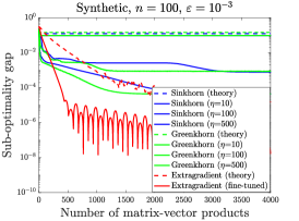
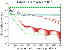
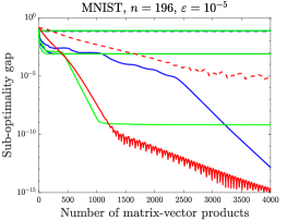
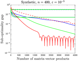
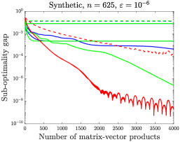
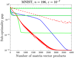
Figure 1: Numerical comparisons of the proposed algorithm, Sinkhorn an Greenkhorn under multiple settings. Each subfigure represents one randomly generated optimal transport problem instance. The legends in the second-to-sixth subfigures are identical to that of the first subfigure, and hence are omitted.

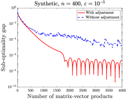
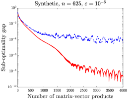
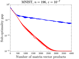
Figure 2: The proposed extragradient method (Algorithm 1) with adjustment step vs. the version without adjustment. The problem instances are the same as those in the second row of Figure 1.

5 Analysis

In this section, we present the proof for our main result: Theorem 1.

5.1 Preliminary facts and additional notation

Before proceeding to the main proof, let us collect several elementary facts concerning the “adjusting” step in our algorithm. Consider any probability vector $\bm{q}=[q_{i}]_{1\leq i\leq d}\in\Delta_{d}$, and transform it into another probability vector $\bm{q}^{\mathsf{adjust}}=[q_{i}^{\mathsf{adjust}}]_{1\leq i\leq d}\in\Delta_{d}$ via the following two steps:

$$q_{i}^{\mathsf{adjust}} =\frac{\max\big{\{}q_{i},\,e^{-B}\|\bm{q}\|_{\infty}\big{\}}}{\sum_{j=1}^{d}\max\big{\{}q_{j},\,e^{-B}\|\bm{q}\|_{\infty}\big{\}}},\qquad i=1,\cdots,d.$$ (32)

We first make note of the following basic property of this transformation:

$$\max_{1\leq i\leq d}\frac{q_{i}}{q_{i}^{\mathsf{adjust}}}\leq 1+de^{-B}.$$ (33)

Proof.

For each $1\leq i\leq d$, it is seen that

$$\frac{q_{i}}{q_{i}^{\mathsf{adjust}}} =\frac{q_{i}}{\max\{q_{i},\,e^{-B}\|\bm{q}\|_{\infty}\}}\cdot\frac{\sum_{j}\max\{q_{j},\,e^{-B}\|\bm{q}\|_{\infty}\}}{\sum_{j}q_{j}}\leq\frac{\sum_{j}\max\{q_{j},\,e^{-B}\|\bm{q}\|_{\infty}\}}{\sum_{j}q_{j}}$$

$$\leq\frac{\sum_{j}q_{j}}{\sum_{j}q_{j}}+\frac{\sum_{j}e^{-B}\|\bm{q}\|_{\infty}}{\sum_{j}q_{j}}\leq 1+de^{-B}\|\bm{q}\|_{\infty}$$

as claimed. ∎

In addition, consider the special two-dimensional case where $\bm{q}=[q_{+},q_{-}]^{\top}\in\Delta_{2}$ and let $\bm{q}^{\mathsf{adjust}}=[q_{+}^{\mathsf{adjust}},q_{-}^{\mathsf{adjust}}]^{\top}\in\Delta_{2}$. If $B>0$, then it holds that

$$\frac{q_{+}^{\mathsf{adjust}}}{q_{-}^{\mathsf{adjust}}}=\begin{cases}\min\big{\{}\frac{q_{+}}{q_{-}},e^{B}\big{\}}\leq e^{B},&\text{if }q_{+}\geq q_{-},\\ \max\big{\{}\frac{q_{+}}{q_{-}},e^{-B}\big{\}}\geq e^{-B},&\text{if }q_{+}<q_{-}.\end{cases}$$ (34)

Proof.

If $q_{+}\geq q_{-}$, then it is readily seen that

$$\frac{q_{+}^{\mathsf{adjust}}}{q_{-}^{\mathsf{adjust}}} =\frac{\max\big{\{}q_{+},e^{-B}q_{+}\big{\}}}{\max\big{\{}q_{-},e^{-B}q_{+}\big{\}}}=\frac{q_{+}}{\max\big{\{}q_{-},e^{-B}q_{+}\big{\}}}=\min\bigg{\{}\frac{q_{+}}{q_{-}},e^{B}\bigg{\}}\leq e^{B}.$$

Similarly, if $q_{+}<q_{-}$, then one can also derive

$$\frac{q_{+}^{\mathsf{adjust}}}{q_{-}^{\mathsf{adjust}}} =\frac{\max\big{\{}q_{+},e^{-B}q_{-}\big{\}}}{\max\big{\{}q_{-},e^{-B}q_{-}\big{\}}}=\frac{\max\big{\{}q_{+},e^{-B}q_{-}\big{\}}}{q_{-}}=\max\bigg{\{}\frac{q_{+}}{q_{-}},e^{-B}\bigg{\}}\geq e^{-B}.$$

∎

Moreover, we would also like to introduce several additional convenient notation that is useful for presenting the proof. Define

$$\bm{\zeta}^{t} \coloneqq\bigg{(}\Big{\{}\frac{1}{\eta_{p,i}}\bm{p}_{i}^{t}\Big{\}}_{i=1}^{n},\Big{\{}\frac{1}{\eta_{\mu,j}}\bm{\mu}_{j}^{t}\Big{\}}_{j=1}^{n}\bigg{)},$$ (35a)

$$\overline{\bm{\zeta}}^{t} \coloneqq\bigg{(}\Big{\{}\frac{1}{\eta_{p,i}}\overline{\bm{p}}_{i}^{t}\Big{\}}_{i=1}^{n},\Big{\{}\frac{1}{\eta_{\mu,j}}\overline{\bm{\mu}}_{j}^{t}\Big{\}}_{j=1}^{n}\bigg{)},$$ (35b)

$$\bm{\zeta}^{t,\mathsf{adjust}} \coloneqq\bigg{(}\Big{\{}\frac{1}{\eta_{p,i}}\bm{p}_{i}^{t}\Big{\}}_{i=1}^{n},\Big{\{}\frac{1}{\eta_{\mu,j}}\bm{\mu}_{j}^{t,\mathsf{adjust}}\Big{\}}_{j=1}^{n}\bigg{)},$$ (35c)

$$\bm{\zeta}^{\star} \coloneqq\bigg{(}\Big{\{}\frac{1}{\eta_{p,i}}\bm{p}_{i}^{\star,\mathsf{reg}}\Big{\}}_{i=1}^{n},\Big{\{}\frac{1}{\eta_{\mu,j}}\bm{\mu}_{j}^{\star,\mathsf{reg}}\Big{\}}_{j=1}^{n}\bigg{)},$$ (35d)

where $\big{\{}\bm{p}_{i}^{\star,\mathsf{reg}}\big{\}}_{i=1}^{n},\big{\{}\bm{\mu}_{j}^{\star,\mathsf{reg}}\big{\}}_{j=1}^{n}$ denotes the optimizer of the entropy-regularized minimax problem (16). Additionally, for any $\bm{\zeta}^{(1)}=\big{(}\{\frac{1}{\eta_{p,i}}\bm{p}_{i}^{(1)}\}_{i=1}^{n},\{\frac{1}{\eta_{\mu,j}}\bm{\mu}_{j}^{(1)}\}_{j=1}^{n}\big{)}$ and $\bm{\zeta}^{(2)}=\big{(}\{\frac{1}{\eta_{p,i}}\bm{p}_{i}^{(2)}\}_{i=1}^{n},\{\frac{1}{\eta_{\mu,j}}\bm{\mu}_{j}^{(2)}\}_{j=1}^{n}\big{)}$ (with the $\bm{p}_{i}^{(1)}$’s, $\bm{p}_{i}^{(2)}$’s, $\bm{\mu}_{i}^{(1)}$’s and $\bm{\mu}_{i}^{(2)}$’s being probability vectors), we introduce a weighted KL divergence metric:

$$\mathsf{KL}_{\mathsf{gen}}\big{(}\bm{\zeta}^{(1)}\parallel\bm{\zeta}^{(2)}\big{)}\coloneqq\sum_{i=1}^{n}\frac{1}{\eta_{p,i}}\mathsf{KL}\big{(}\bm{p}^{(1)}_{i}\parallel\bm{p}^{(2)}_{i}\big{)}+\sum_{j=1}^{n}\frac{1}{\eta_{\mu,j}}\mathsf{KL}\big{(}\bm{\mu}^{(1)}_{j}\parallel\bm{\mu}^{(2)}_{j}\big{)}.$$ (36)

5.2 Proof of Theorem 1

We are now positioned to prove Theorem 1. To begin with, we make the observation that

$$\mathsf{KL}(\bm{\mu}_{j}^{\star,\mathsf{reg}}\parallel\bm{\mu}_{j}^{t,\mathsf{adjust}}) =\sum_{s\in\{+,-\}}\mu_{j,s}^{\star,\mathsf{reg}}\log\frac{\mu_{j,s}^{\star,\mathsf{reg}}}{\mu_{j,s}^{t,\mathsf{adjust}}}=\sum_{s\in\{+,-\}}\mu_{j,s}^{\star,\mathsf{reg}}\log\frac{\mu_{j,s}^{\star,\mathsf{reg}}}{\mu_{j,s}^{t}}+\sum_{s\in\{+,-\}}\mu_{j,s}^{\star,\mathsf{reg}}\log\frac{\mu_{j,s}^{t}}{\mu_{j,s}^{t,\mathsf{adjust}}}$$

$$\leq\mathsf{KL}(\bm{\mu}_{j}^{\star,\mathsf{reg}}\parallel\bm{\mu}_{j}^{t})+\sum_{s\in\{+,-\}}\mu_{j,s}^{\star,\mathsf{reg}}\log\max\left\{\frac{\mu_{j,+}^{t}}{\mu_{j,+}^{t,\mathsf{adjust}}},\frac{\mu_{j,-}^{t}}{\mu_{j,-}^{t,\mathsf{adjust}}}\right\}$$

$$\leq\mathsf{KL}(\bm{\mu}_{j}^{\star,\mathsf{reg}}\parallel\bm{\mu}_{j}^{t})+\log\big{(}1+2e^{-B}\big{)},$$

where the last inequality arises from the relation (33) and the fact that $\sum_{s\in\{+,-\}}\mu_{j,s}^{\star,\mathsf{reg}}=1$. As a result, combine the above inequality with the definitions (35c) and (35a) to arrive at

$$\mathsf{KL}_{\mathsf{gen}}\big{(}\bm{\zeta}^{\star}\parallel\bm{\zeta}^{t,\mathsf{adjust}}\big{)} =\sum_{i=1}^{n}\frac{1}{\eta_{p,i}}\mathsf{KL}\big{(}\bm{p}_{i}^{\star,\mathsf{reg}}\parallel\bm{p}_{i}^{t}\big{)}+\sum_{j=1}^{n}\frac{1}{\eta_{\mu,j}}\mathsf{KL}\big{(}\bm{\mu}_{j}^{\star,\mathsf{reg}}\parallel\bm{\mu}_{j}^{t,\mathsf{adjust}}\big{)}$$

$$\leq\sum_{i=1}^{n}\frac{1}{\eta_{p,i}}\mathsf{KL}\big{(}\bm{p}_{i}^{\star,\mathsf{reg}}\parallel\bm{p}_{i}^{t}\big{)}+\sum_{j=1}^{n}\frac{1}{\eta_{\mu,j}}\mathsf{KL}\big{(}\bm{\mu}_{j}^{\star,\mathsf{reg}}\parallel\bm{\mu}_{j}^{t}\big{)}+\log\big{(}1+2e^{-B}\big{)}\sum_{j=1}^{n}\frac{1}{\eta_{\mu,j}}$$

$$=\mathsf{KL}_{\mathsf{gen}}\big{(}\bm{\zeta}^{\star}\parallel\bm{\zeta}^{t}\big{)}+\log\big{(}1+2e^{-B}\big{)}\cdot\sum_{j=1}^{n}\frac{c_{j}+C_{3}/n}{15C_{2}\sqrt{B}}$$

$$=\mathsf{KL}_{\mathsf{gen}}\big{(}\bm{\zeta}^{\star}\parallel\bm{\zeta}^{t}\big{)}+\frac{1+C_{3}}{15C_{2}\sqrt{C_{1}\log\frac{n}{\varepsilon}}}\log\big{(}1+2e^{-B}\big{)}$$

$$\leq\mathsf{KL}_{\mathsf{gen}}\big{(}\bm{\zeta}^{\star}\parallel\bm{\zeta}^{t}\big{)}+e^{-B},$$ (37)

where the third line results from the choice (25), the penultimate line relies on $\sum_{j}c_{j}=1$, and the last line makes use of $\log(1+x)\leq x$ for all $x\geq 0$ and holds if $C_{2}\sqrt{C_{1}}$ is sufficiently large (recall that $C_{3}\leq 1$). In a nutshell, (37) indicates that the KL divergence between the optimal point and the $t$-th iterate is not increased by much when $\bm{\zeta}^{t}$ is replaced with $\bm{\zeta}^{t,\mathsf{adjust}}$.

The next step consists of establishing the following result that monitors the change of KL divergence when $\bm{\zeta}^{t,\mathsf{adjust}}$ is further replaced with $\bm{\zeta}^{t+1}$:

$$\mathsf{KL}_{\mathsf{gen}}\big{(}\bm{\zeta}^{\star}\parallel\bm{\zeta}^{t+1}\big{)}\leq(1-\eta)\mathsf{KL}_{\mathsf{gen}}\big{(}\bm{\zeta}^{\star}\parallel\bm{\zeta}^{t,\mathsf{adjust}}\big{)}+8ne^{-B},\qquad\forall t\geq 0.$$ (38)

Crucially, a contraction factor of $1-\eta$ appears in the above claim, revealing the progress made per iteration. Suppose for the moment that this claim (38) is valid. Then taking it together with (37) gives

$$\mathsf{KL}_{\mathsf{gen}}\big{(}\bm{\zeta}^{\star}\parallel\bm{\zeta}^{t+1}\big{)}\leq(1-\eta)\mathsf{KL}_{\mathsf{gen}}\big{(}\bm{\zeta}^{\star}\parallel\bm{\zeta}^{t}\big{)}+(8n+1)e^{-B},\qquad\forall t\geq 0.$$ (39)

Applying this relation recursively further implies that

$$\mathsf{KL}_{\mathsf{gen}}\big{(}\bm{\zeta}^{\star}\parallel\bm{\zeta}^{t_{\max}}\big{)} \leq(1-\eta)^{t_{\max}}\mathsf{KL}_{\mathsf{gen}}\big{(}\bm{\zeta}^{\star}\parallel\bm{\zeta}^{0}\big{)}+(8n+1)e^{-B}\sum_{t=0}^{t_{\max}-1}(1-\eta)^{t}$$

$$\leq(1-\eta)^{t_{\max}}\mathsf{KL}_{\mathsf{gen}}\big{(}\bm{\zeta}^{\star}\parallel\bm{\zeta}^{0}\big{)}+\frac{(8n+1)e^{-B}}{\eta}.$$ (40)

Regarding the first term in (40), it is observed from our initialization (cf. line 1 of Algorithm 1) that

$$\begin{cases}\mathsf{KL}\big{(}\bm{p}_{i}^{\star,\mathsf{reg}}\parallel\bm{p}_{i}^{0}\big{)}&=-\mathcal{H}\big{(}\bm{p}_{i}^{\star,\mathsf{reg}}\big{)}+\sum_{j=1}^{n}p_{i,j}^{\star,\mathsf{reg}}\log\frac{1}{p_{i,j}^{0}}\leq\sum_{j=1}^{n}p_{i,j}^{\star,\mathsf{reg}}\log n=\log n,\\ \mathsf{KL}\big{(}\bm{\mu}_{j}^{\star,\mathsf{reg}}\parallel\bm{\mu}_{j}^{0}\big{)}&=-\mathcal{H}\big{(}\bm{\mu}_{j}^{\star,\mathsf{reg}}\big{)}+\sum_{s\in\{+,-\}}\mu_{j,s}^{\star,\mathsf{reg}}\log\frac{1}{\mu_{j,s}^{0}}\leq\sum_{s\in\{+,-\}}\mu_{j,s}^{\star,\mathsf{reg}}\log 2=\log 2,\end{cases}$$

and consequently,

$$\mathsf{KL}_{\mathsf{gen}}\big{(}\bm{\zeta}^{\star}\parallel\bm{\zeta}^{0}\big{)}\leq\sum_{i=1}^{n}\frac{\log n}{\eta_{p,i}}+\sum_{j=1}^{n}\frac{\log 2}{\eta_{\mu,j}}=\frac{\sqrt{B}\log n}{C_{2}}\sum_{i=1}^{n}r_{i}+\frac{\log 2}{15C_{2}\sqrt{B}}\sum_{j=1}^{n}\Big{(}c_{j}+\frac{C_{3}}{n}\Big{)}\leq\frac{2\sqrt{B}\log n}{C_{2}},$$

where we recall that $0<C_{3}\leq 1$. This in turn leads to $(1-\eta)^{t_{\max}}\mathsf{KL}_{\mathsf{gen}}\big{(}\bm{\zeta}^{\star}\parallel\bm{\zeta}^{0}\big{)}\leq\varepsilon^{2}$, provided that $t_{\max}\geq C_{4}\frac{1}{\eta}\log\frac{n}{\varepsilon}$ for some large enough constant $C_{4}>0$. Turning to the second term in (40), one utilizes $B=C_{1}\log\frac{n}{\varepsilon}$ to obtain

$$\frac{(8n+1)e^{-B}}{\eta}=\frac{(8n+1)e^{-B}\sqrt{B}\log n}{C_{2}^{2}\varepsilon}\leq\frac{(8n+1)e^{-\frac{1}{2}B}\log n}{C_{2}^{2}\varepsilon}=\frac{(8n+1)e^{-\frac{1}{2}C_{1}\log\frac{n}{\varepsilon}}\log n}{C_{2}^{2}\varepsilon}\leq\varepsilon^{2},$$

with the proviso that $C_{1}>0$ is sufficiently large. Substitution into (40) thus yields

$$\mathsf{KL}_{\mathsf{gen}}\big{(}\bm{\zeta}^{\star}\parallel\bm{\zeta}^{t_{\max}}\big{)} \leq\varepsilon^{2}+\varepsilon^{2}=2\varepsilon^{2}.$$ (41)

As it turns out, it is more convenient to work with the $\ell_{1}$-based error. To convert the above bound on KL divergence into $\ell_{1}$-based distance, one invokes Pinsker’s inequality (Tsybakov,, 2009, Lemma 2.5) to reach

$$\big{\|}\widehat{\bm{P}}-\bm{P}^{\star,\mathsf{reg}}\big{\|}_{1} =\sum_{i=1}^{n}r_{i}\big{\|}\bm{p}_{i}^{\star,\mathsf{reg}}-\bm{p}_{i}^{\star,t_{\max}}\big{\|}_{1}\leq\sum_{i=1}^{n}r_{i}\sqrt{2\mathsf{KL}\big{(}\bm{p}_{i}^{\star,\mathsf{reg}}\parallel\bm{p}_{i}^{t_{\max}}\big{)}}$$

$$\leq\left\{\sum_{i=1}^{n}r_{i}\right\}^{\frac{1}{2}}\left\{2\sum_{i=1}^{n}r_{i}\mathsf{KL}\big{(}\bm{p}_{i}^{\star,\mathsf{reg}}\parallel\bm{p}_{i}^{t_{\max}}\big{)}\right\}^{\frac{1}{2}}$$

$$=\left\{2\sum_{i=1}^{n}r_{i}\mathsf{KL}\big{(}\bm{p}_{i}^{\star,\mathsf{reg}}\parallel\bm{p}_{i}^{t_{\max}}\big{)}\right\}^{\frac{1}{2}}$$

$$=\left\{\frac{2C_{2}}{\sqrt{B}}\sum_{i=1}^{n}\frac{1}{\eta_{p,i}}\mathsf{KL}\big{(}\bm{p}_{i}^{\star,\mathsf{reg}}\parallel\bm{p}_{i}^{t_{\max}}\big{)}\right\}^{\frac{1}{2}}$$

$$\leq\left\{\frac{2C_{2}}{\sqrt{C_{1}\log\frac{n}{\varepsilon}}}\mathsf{KL}_{\mathsf{gen}}\big{(}\bm{\zeta}^{\star}\parallel\bm{\zeta}^{t_{\max}}\big{)}\right\}^{\frac{1}{2}}\leq\frac{\varepsilon}{6}.$$ (42)

Here, the first inequality invokes Pinsker’s inequality, the second inequality results from Cauchy-Schwarz, the third line holds since $\sum_{i}r_{i}=1$, the fourth line uses the choice (24) of $\eta_{p,i}$, whereas the last line results from the definition (36) and the bound (41) and is valid as long as $C_{2}$ (resp. $C_{1}$) is sufficiently small (resp. large).

Thus far, we have demonstrated fast convergence of our algorithm to the solution to the entropy-regularized problem (16). To finish up, we still need to show the proximity of the objective values under the regularized solution $\bm{P}^{\star,\mathsf{reg}}$ and under the true optimizer $\bm{P}^{\star}$. For notational convenience, define

$$\overline{\bm{\mu}}_{j}^{\star}\coloneqq\arg\max_{\bm{\mu}_{j}\in\Delta_{2}}f\big{(}\{\bm{p}_{i}^{\star,\mathsf{reg}}\}_{i=1}^{n},\{\bm{\mu}_{j}\}_{i=1}^{n}\big{)},\qquad 1\leq j\leq n.$$ (43)

Given that $\sum_{j=1}^{n}\tau_{\mu,j}\log 2+\sum_{i=1}^{n}\tau_{p,i}\log n\leq\varepsilon/4$ under our choice (26) (see (27) as long as $C_{2}/C_{1}$ is sufficiently small), we obtain

$$\frac{1}{2}\langle\bm{W},\bm{P}^{\star,\mathsf{reg}}\rangle+\big{\|}\bm{P}^{\star,\mathsf{reg}}\bm{1}-\bm{c}\big{\|}_{1} =f\big{(}\{\bm{p}_{i}^{\star,\mathsf{reg}}\}_{i=1}^{n},\{\overline{\bm{\mu}}_{j}^{\star}\}_{i=1}^{n}\big{)}$$

$$\leq F\big{(}\{\bm{p}_{i}^{\star,\mathsf{reg}}\}_{i=1}^{n},\{\overline{\bm{\mu}}_{j}^{\star}\}_{i=1}^{n}\big{)}+\sum_{i=1}^{n}\tau_{p,i}\log n$$

$$\leq F\big{(}\{\bm{p}_{i}^{\star,\mathsf{reg}}\}_{i=1}^{n},\{\bm{\mu}_{j}^{\star,\mathsf{reg}}\}_{i=1}^{n}\big{)}+\sum_{i=1}^{n}\tau_{p,i}\log n$$

$$\leq F\big{(}\{\bm{p}_{i}^{\star}\}_{i=1}^{n},\{\bm{\mu}_{j}^{\star,\mathsf{reg}}\}_{i=1}^{n}\big{)}+\sum_{i=1}^{n}\tau_{p,i}\log n$$

$$\leq f\big{(}\{\bm{p}_{i}^{\star}\}_{i=1}^{n},\{\bm{\mu}_{j}^{\star,\mathsf{reg}}\}_{i=1}^{n}\big{)}+\sum_{i=1}^{n}\tau_{p,i}\log n+\sum_{j=1}^{n}\tau_{\mu,j}\log 2$$

$$\leq\max_{\bm{\mu}_{j}\in\Delta_{2},\forall j}f\big{(}\{\bm{p}_{i}^{\star}\}_{i=1}^{n},\{\bm{\mu}_{j}\}_{i=1}^{n}\big{)}+\sum_{i=1}^{n}\tau_{p,i}\log n+\sum_{j=1}^{n}\tau_{\mu,j}\log 2$$

$$=\frac{1}{2}\langle\bm{W},\bm{P}^{\star}\rangle+\bigg{\|}\sum_{i=1}^{n}r_{i}\bm{p}_{i}^{\star}-\bm{c}\bigg{\|}_{1}+\sum_{i=1}^{n}\tau_{p,i}\log n+\sum_{j=1}^{n}\tau_{\mu,j}\log 2$$

$$\leq\frac{1}{2}\langle\bm{W},\bm{P}^{\star}\rangle+\frac{\varepsilon}{4}.$$ (44)

Here, the first identity comes from (12) and the definition of $\overline{\bm{\mu}}_{j}^{\star}$, the second line is valid since $\mathcal{H}(\bm{p}_{i}^{\star,\mathsf{adjust}})\leq\log n$ for all $1\leq i\leq n$, the third and the fourth lines hold since $\big{(}\{\bm{p}_{i}^{\star,\mathsf{reg}}\}_{i=1}^{n},\{\bm{\mu}_{j}^{\star,\mathsf{reg}}\}_{i=1}^{n}\big{)}$ corresponds to the minimax solution of $F(\cdot,\cdot)$, the fifth line relies on $\mathcal{H}(\bm{\mu}_{j}^{\star,\mathsf{adjust}})\leq\log 2$ for all $1\leq j\leq n$, the penultimate line arises from (12), while the last line results from the fact $\sum_{i}r_{i}\bm{p}_{i}^{\star}=\bm{c}$ and the assumption $\sum_{j=1}^{n}\tau_{\mu,j}\log 2+\sum_{i=1}^{n}\tau_{p,i}\log n\leq\varepsilon/4$. As a consequence, we are ready to conclude that

$$\langle\bm{W},\widetilde{\bm{P}}\rangle \leq\langle\bm{W},\widehat{\bm{P}}\rangle+\|\bm{W}\|_{\infty}\|\widehat{\bm{P}}-\widetilde{\bm{P}}\|_{1}$$

$$\leq\langle\bm{W},\widehat{\bm{P}}\rangle+2\big{\|}\widehat{\bm{P}}\bm{1}-\bm{c}\big{\|}_{1}$$

$$\leq\langle\bm{W},\bm{P}^{\star,\mathsf{reg}}\rangle+\|\bm{W}\|_{\infty}\big{\|}\widehat{\bm{P}}-\bm{P}^{\star,\mathsf{reg}}\big{\|}_{1}+2\big{\|}\bm{P}^{\star,\mathsf{reg}}\bm{1}-\bm{c}\big{\|}_{1}+2\big{\|}\widehat{\bm{P}}-\bm{P}^{\star,\mathsf{reg}}\big{\|}_{1}\|\bm{1}\|_{\infty}$$

$$=\langle\bm{W},\bm{P}^{\star,\mathsf{reg}}\rangle+2\big{\|}\bm{P}^{\star,\mathsf{reg}}\bm{1}-\bm{c}\big{\|}_{1}+3\big{\|}\widehat{\bm{P}}-\bm{P}^{\star,\mathsf{reg}}\big{\|}_{1}$$

$$\leq\langle\bm{W},\bm{P}^{\star}\rangle+\varepsilon/2+\varepsilon/2=\langle\bm{W},\bm{P}^{\star}\rangle+\varepsilon,$$

where the second inequality invokes Lemma 1, the assumption $\|\bm{W}\|_{\infty}=1$, and the fact $\widehat{\bm{P}}\bm{1}=\bm{r}$, and the last inequality arises from (42) and (44). This establishes the advertised result in Theorem 1.

The remainder of the proof is thus dedicated to establishing the claim (38), detailed in the next subsection.

5.3 Proof of Claim (38)

5.3.1 Step 1: decomposing the KL divergence of interest

Elementary calculation together with the definition (36) of $\mathsf{KL}_{\mathsf{gen}}(\cdot\parallel\cdot)$ reveals that

$$(1-\eta)\mathsf{KL}_{\mathsf{gen}}\big{(}\bm{\zeta}^{\star}\parallel\bm{\zeta}^{t,\mathsf{adjust}}\big{)}-(1-\eta)\mathsf{KL}_{\mathsf{gen}}\big{(}\overline{\bm{\zeta}}^{t+1}\parallel\bm{\zeta}^{t,\mathsf{adjust}}\big{)}-\eta\mathsf{KL}_{\mathsf{gen}}\big{(}\overline{\bm{\zeta}}^{t+1}\parallel\bm{\zeta}^{\star}\big{)}-\mathsf{KL}_{\mathsf{gen}}\big{(}\bm{\zeta}^{t+1}\parallel\overline{\bm{\zeta}}^{t+1}\big{)}$$

$$\qquad+\big{\langle}\overline{\bm{\zeta}}^{t+1}-\bm{\zeta}^{t+1},\,\log\overline{\bm{\zeta}}^{t+1}-\log\bm{\zeta}^{t+1}\big{\rangle}+\big{\langle}\overline{\bm{\zeta}}^{t+1}-\bm{\zeta}^{\star},\,\log\bm{\zeta}^{t+1}-(1-\eta)\log\bm{\zeta}^{t,\mathsf{adjust}}-\eta\log\bm{\zeta}^{\star}\big{\rangle}$$

$$=(1-\eta)\big{\langle}\bm{\zeta}^{\star},\,\log\bm{\zeta}^{\star}-\log\bm{\zeta}^{t,\mathsf{adjust}}\big{\rangle}-(1-\eta)\big{\langle}\overline{\bm{\zeta}}^{t+1},\,\log\overline{\bm{\zeta}}^{t+1}-\log\bm{\zeta}^{t,\mathsf{adjust}}\big{\rangle}$$

$$\qquad-\eta\big{\langle}\overline{\bm{\zeta}}^{t+1},\,\log\overline{\bm{\zeta}}^{t+1}-\log\bm{\zeta}^{\star}\big{\rangle}-\big{\langle}\bm{\zeta}^{t+1},\,\log\bm{\zeta}^{t+1}-\log\overline{\bm{\zeta}}^{t+1}\big{\rangle}$$

$$\qquad+\big{\langle}\overline{\bm{\zeta}}^{t+1}-\bm{\zeta}^{t+1},\,\log\overline{\bm{\zeta}}^{t+1}-\log\bm{\zeta}^{t+1}\big{\rangle}+\big{\langle}\overline{\bm{\zeta}}^{t+1}-\bm{\zeta}^{\star},\,\log\bm{\zeta}^{t+1}-(1-\eta)\log\bm{\zeta}^{t,\mathsf{adjust}}-\eta\log\bm{\zeta}^{\star}\big{\rangle}$$

$$=\big{\langle}\bm{\zeta}^{\star},\,\log\bm{\zeta}^{\star}\big{\rangle}-\big{\langle}\bm{\zeta}^{\star},\,\log\bm{\zeta}^{t+1}\big{\rangle}=\mathsf{KL}_{\mathsf{gen}}\big{(}\bm{\zeta}^{\star}\parallel\bm{\zeta}^{t+1}\big{)};$$ (45)

here and throughout, the logarithmic operator in $\log\bm{\zeta}$ is applied in an entrywise manner. In addition, inspired by Cen et al., (2021, Lemma 1), we observe that

$$\big{\langle}\overline{\bm{\zeta}}^{t+1}-\bm{\zeta}^{\star},\,\log\bm{\zeta}^{t+1}-(1-\eta)\log\bm{\zeta}^{t,\mathsf{adjust}}-\eta\log\bm{\zeta}^{\star}\big{\rangle}=0;$$ (46)

see Appendix B for the proof of this relation. Substitution into (45) leads to

$$\mathsf{KL}_{\mathsf{gen}}\big{(}\bm{\zeta}^{\star}\parallel\bm{\zeta}^{t+1}\big{)} =(1-\eta)\mathsf{KL}_{\mathsf{gen}}\big{(}\bm{\zeta}^{\star}\parallel\bm{\zeta}^{t,\mathsf{adjust}}\big{)}-(1-\eta)\mathsf{KL}_{\mathsf{gen}}\big{(}\overline{\bm{\zeta}}^{t+1}\parallel\bm{\zeta}^{t,\mathsf{adjust}}\big{)}-\eta\mathsf{KL}_{\mathsf{gen}}\big{(}\overline{\bm{\zeta}}^{t+1}\parallel\bm{\zeta}^{\star}\big{)}$$

$$\qquad\qquad-\mathsf{KL}_{\mathsf{gen}}\big{(}\bm{\zeta}^{t+1}\parallel\overline{\bm{\zeta}}^{t+1}\big{)}+\big{\langle}\overline{\bm{\zeta}}^{t+1}-\bm{\zeta}^{t+1},\,\log\overline{\bm{\zeta}}^{t+1}-\log\bm{\zeta}^{t+1}\big{\rangle}.$$ (47)

Everything then boils down to controlling the inner product term $\big{\langle}\overline{\bm{\zeta}}^{t+1}-\bm{\zeta}^{t+1},\,\log\overline{\bm{\zeta}}^{t+1}-\log\bm{\zeta}^{t+1}\big{\rangle}$.

Towards this end, we first invoke the update rules (19) and (20) to yield

$$\big{\langle}\overline{\bm{\zeta}}^{t+1}-\bm{\zeta}^{t+1},\,\log\overline{\bm{\zeta}}^{t+1}-\log\bm{\zeta}^{t+1}\big{\rangle} =\sum_{j=1}^{n}\big{(}\overline{\mu}_{j,+}^{t+1}-\overline{\mu}_{j,-}^{t+1}-\mu_{j,+}^{t+1}+\mu_{j,-}^{t+1}\big{)}\bigg{\{}\sum_{i=1}^{n}r_{i}\big{(}p_{i,j}^{t}-\overline{p}_{i,j}^{t+1}\big{)}\bigg{\}}$$

$$\quad+\sum_{j=1}^{n}\big{(}\overline{\mu}_{j,+}^{t+1}-\overline{\mu}_{j,-}^{t+1}-\mu_{j,+}^{t,\mathsf{adjust}}+\mu_{j,-}^{t,\mathsf{adjust}}\big{)}\bigg{\{}\sum_{i=1}^{n}r_{i}\big{(}\overline{p}_{i,j}^{t+1}-p_{i,j}^{t+1}\big{)}\bigg{\}},$$ (48)

whose proof is also deferred to Appendix B. In order to bound the two sums on the right-hand side of (48), we find it convenient to first introduce the following index subset:

$$\mathcal{J}_{t}\coloneqq\bigg{\{}j:\sum_{i=1}^{n}r_{i}p_{i,j}^{t}<2e\Big{(}c_{j}+\frac{1}{n}\Big{)}\bigg{\}}.$$ (49)

We then divide each sum into two parts — $\big{\{}j:j\in\mathcal{J}_{t}\big{\}}$ and $\big{\{}j:j\notin\mathcal{J}_{t}\big{\}}$ — and look at them separately.

5.3.2 Step 2: controlling terms with $j\in\mathcal{J}_{t}$

We start by looking at those terms with $j\in\mathcal{J}_{t}$. With regards to the first sum on the right-hand side of (48), we have

$$\sum_{j\in\mathcal{J}_{t}}\big{(}\overline{\mu}_{j,+}^{t+1}-\overline{\mu}_{j,-}^{t+1}-\mu_{j,+}^{t+1}+\mu_{j,-}^{t+1}\big{)}\bigg{\{}\sum_{i=1}^{n}r_{i}\big{(}p_{i,j}^{t}-\overline{p}_{i,j}^{t+1}\big{)}\bigg{\}}$$

$$\qquad\leq\sum_{j\in\mathcal{J}_{t}}\frac{1}{2\eta_{\mu,j}}\big{(}\overline{\mu}_{j,+}^{t+1}-\overline{\mu}_{j,-}^{t+1}-\mu_{j,+}^{t+1}+\mu_{j,-}^{t+1}\big{)}^{2}+\sum_{j\in\mathcal{J}_{t}}\frac{\eta_{\mu,j}}{2}\bigg{\{}\sum_{i=1}^{n}r_{i}\big{(}p_{i,j}^{t}-\overline{p}_{i,j}^{t+1}\big{)}\bigg{\}}^{2}.$$ (50)

Recognizing that $\overline{\bm{\mu}}_{j}^{t+1},\bm{\mu}_{j}^{t+1}\in\Delta_{2}$, one can invoke Pinsker’s inequality (Tsybakov,, 2009, Lemma 2.5) to bound the first term on the right-hand side of (50) as follows:

$$\big{(}\overline{\mu}_{j,+}^{t+1}-\overline{\mu}_{j,-}^{t+1}-\mu_{j,+}^{t+1}+\mu_{j,-}^{t+1}\big{)}^{2} =\big{\|}\overline{\bm{\mu}}_{j}^{t+1}-\bm{\mu}_{j}^{t+1}\big{\|}_{1}^{2}\leq 2\mathsf{KL}\big{(}\bm{\mu}_{j}^{t+1}\parallel\overline{\bm{\mu}}_{j}^{t+1}\big{)}.$$ (51)

Regarding the second term on the right-hand side of (50), we see that, for $\eta<1/2$,

$$\sum_{i}(1-\eta)\frac{1}{\eta_{p,i}}\mathsf{KL}\big{(}\overline{\bm{p}}_{i}^{t+1}\parallel\bm{p}_{i}^{t}\big{)}\geq\frac{1}{2}\sum_{i=1}^{n}\sum_{j=1}^{n}\frac{\overline{p}_{i,j}^{t+1}}{\eta_{p,i}}\log\frac{\overline{p}_{i,j}^{t+1}}{p_{i,j}^{t}}$$ (52)

$$\qquad\geq\frac{1}{2\max_{i}\eta_{p,i}r_{i}}\sum_{i=1}^{n}\sum_{j=1}^{n}r_{i}p_{i,j}^{t}\big{(}(1+x_{ij})\log(1+x_{i,j})\big{)}$$

$$\qquad\overset{\mathrm{(i)}}{=}\frac{1}{2\max_{i}\eta_{p,i}r_{i}}\sum_{j=1}^{n}\sum_{i=1}^{n}r_{i}p_{i,j}^{t}\big{(}(1+x_{ij})\log(1+x_{i,j})-x_{i,j}\big{)}$$

$$\qquad\overset{\mathrm{(ii)}}{\geq}\frac{3}{4\max_{i}\eta_{p,i}r_{i}}\sum_{j=1}^{n}\frac{1}{2\sum_{i=1}^{n}r_{i}p_{i,j}^{t}+\sum_{i=1}^{n}r_{i}\overline{p}_{i,j}^{t+1}}\bigg{\{}\sum_{i=1}^{n}r_{i}\big{(}p_{i,j}^{t}-\overline{p}_{i,j}^{t+1}\big{)}\bigg{\}}^{2}$$

$$\qquad\overset{\mathrm{(iii)}}{\geq}\frac{1}{20e\big{(}\max_{i}\eta_{p,i}r_{i}\big{)}\big{(}\max_{j}\eta_{\mu,j}(c_{j}+1/n)\big{)}}\sum_{j\in\mathcal{J}_{t}}\eta_{\mu,j}\bigg{\{}\sum_{i=1}^{n}r_{i}\big{(}p_{i,j}^{t}-\overline{p}_{i,j}^{t+1}\big{)}\bigg{\}}^{2},$$ (53)

where we define $x_{i,j}\coloneqq\frac{\overline{p}_{i,j}^{t+1}}{p_{i,j}^{t}}-1$. Here, (i) is valid due to $\sum_{j}p_{i,j}^{t}x_{i,j}=\sum_{j}(\overline{p}_{i,j}^{t}-p_{i,j}^{t})=0$; (ii) arises since

$$\sum_{i=1}^{n}r_{i}p_{i,j}^{t}\big{(}(1+x_{i,j})\log(1+x_{i,j})-x_{i,j}\big{)}\geq\frac{1}{2}\sum_{i=1}^{n}r_{i}p_{i,j}^{t}\frac{x_{i,j}^{2}}{1+x_{i,j}/3}=\frac{1}{2}\sum_{i=1}^{n}\frac{(r_{i}p_{i,j}^{t})^{2}x_{i,j}^{2}}{r_{i}p_{i,j}^{t}(1+x_{i,j}/3)}$$

$$\quad\geq\frac{1}{2}\frac{1}{\sum_{i=1}^{n}r_{i}p_{i,j}^{t}(1+x_{i,j}/3)}\Big{(}\sum_{i=1}^{n}r_{i}p_{i,j}^{t}x_{i,j}\Big{)}^{2}=\frac{3}{4\sum_{i=1}^{n}r_{i}p_{i,j}^{t}+2\sum_{i=1}^{n}r_{i}\overline{p}_{i,j}^{t+1}}\Big{(}\sum_{i=1}^{n}r_{i}\big{(}\overline{p}_{i,j}^{t+1}-p_{i,j}^{t}\big{)}\Big{)}^{2},$$

where the first inequality holds since $(1+z)\log(1+z)-z\geq\frac{z^{2}}{2(1+z/3)}$ for all $z\geq-1$, and the second line follows from Sedrakyan’s inequality (Sedrakyan and Sedrakyan,, 2018, Chapter 8, Lemma 1); (iii) comes from the definition (49) of $\mathcal{J}_{t}$, as well as the following claim (which will be proved momentarily):

$$\sum_{i=1}^{n}r_{i}\overline{p}_{i,j}^{t+1}<5e\Big{(}c_{j}+\frac{1}{n}\Big{)}\qquad\text{and}\qquad\sum_{i=1}^{n}r_{i}p_{i,j}^{t+1}<5e\Big{(}c_{j}+\frac{1}{n}\Big{)},\qquad\forall j\in\mathcal{J}_{t}.$$ (54)

Substituting (51) and (53) into (50) yields

$$\sum_{j\in\mathcal{J}_{t}}\big{(}\overline{\mu}_{j,+}^{t+1}-\overline{\mu}_{j,-}^{t+1}-\mu_{j,+}^{t+1}+\mu_{j,-}^{t+1}\big{)}\bigg{\{}\sum_{i=1}^{n}r_{i}\big{(}p_{i,j}^{t}-\overline{p}_{i,j}^{t+1}\big{)}\bigg{\}}$$

$$\leq\sum_{j\in\mathcal{J}_{t}}\frac{1}{\eta_{\mu,j}}\mathsf{KL}\big{(}\bm{\mu}_{j}^{t+1}\parallel\overline{\bm{\mu}}_{j}^{t+1}\big{)}+(1-\eta)40e\Big{(}\max_{i}\eta_{p,i}r_{i}\Big{)}\Big{(}\max_{j}\eta_{\mu,j}(c_{j}+1/n)\Big{)}\sum_{i}\frac{1}{\eta_{p,i}}\mathsf{KL}\big{(}\overline{\bm{p}}_{i}^{t+1}\parallel\bm{p}_{i}^{t}\big{)}$$

$$\leq\sum_{j\in\mathcal{J}_{t}}\frac{1}{\eta_{\mu,j}}\mathsf{KL}\big{(}\bm{\mu}_{j}^{t+1}\parallel\overline{\bm{\mu}}_{j}^{t+1}\big{)}+(1-\eta)\sum_{i}\frac{1}{\eta_{p,i}}\mathsf{KL}\big{(}\overline{\bm{p}}_{i}^{t+1}\parallel\bm{p}_{i}^{t}\big{)},$$ (55)

provided that (using the choice (25) and the assumption $0<C_{3}\leq 1$)

$$\Big{(}\max_{i}\eta_{p,i}r_{i}\Big{)}\Big{(}\max_{j}\eta_{\mu,j}(c_{j}+1/n)\Big{)}\leq\frac{1}{C_{3}}\Big{(}\max_{i}\eta_{p,i}r_{i}\Big{)}\Big{(}\max_{j}\eta_{\mu,j}(c_{j}+C_{3}/n)\Big{)}=\frac{15C_{2}^{2}}{C_{3}}\leq\frac{1}{40e}.$$ (56)

We then move on to the second sum on the right-hand side of (48) when restricted to $\mathcal{J}_{t}$. Repeating the arguments as above, we can guarantee that

$$\sum_{j\in\mathcal{J}_{t}}\big{(}\overline{\mu}_{j,+}^{t+1}-\overline{\mu}_{j,-}^{t+1}-\mu_{j,+}^{t,\mathsf{adjust}}+\mu_{j,-}^{t,\mathsf{adjust}}\big{)}\sum_{i=1}^{n}r_{i}\big{(}\overline{p}_{i,j}^{t+1}-p_{i,j}^{t+1}\big{)}$$

$$\qquad\leq\sum_{j\in\mathcal{J}_{t}}\frac{1-\eta}{2\eta_{\mu,j}}\big{(}\overline{\mu}_{j,+}^{t+1}-\overline{\mu}_{j,-}^{t+1}-\mu_{j,+}^{t,\mathsf{adjust}}+\mu_{j,-}^{t,\mathsf{adjust}}\big{)}^{2}+\frac{1}{2(1-\eta)}\sum_{j\in\mathcal{J}_{t}}\eta_{\mu,j}\bigg{\{}\sum_{i=1}^{n}r_{i}\big{(}\overline{p}_{i,j}^{t+1}-p_{i,j}^{t+1}\big{)}\bigg{\}}^{2}$$

$$\qquad\leq\sum_{j}\frac{1-\eta}{\eta_{\mu,j}}\mathsf{KL}\big{(}\overline{\bm{\mu}}_{j}^{t+1}\parallel\bm{\mu}_{j}^{t,\mathsf{adjust}}\big{)}+\sum_{i}\frac{1}{\eta_{p,i}}\mathsf{KL}\big{(}\bm{p}_{i}^{t+1}\parallel\overline{\bm{p}}_{i}^{t+1}\big{)},$$

as long as $0<\eta<1/2$ (so that $\frac{1}{1-\eta}\leq 2$) and Condition (56) is met; the details are omitted here for brevity. Combining this result with (55), we reach

$$\sum_{j\in\mathcal{J}_{t}}\big{(}\overline{\mu}_{j,+}^{t+1}-\overline{\mu}_{j,-}^{t+1}-\mu_{j,+}^{t+1}+\mu_{j,-}^{t+1}\big{)}\sum_{i=1}^{n}r_{i}\big{(}p_{i,j}^{t}-\overline{p}_{i,j}^{t+1}\big{)}$$

$$\qquad\qquad+\sum_{j\in\mathcal{J}_{t}}\big{(}\overline{\mu}_{j,+}^{t+1}-\overline{\mu}_{j,-}^{t+1}-\mu_{j,+}^{t,\mathsf{adjust}}+\mu_{j,-}^{t,\mathsf{adjust}}\big{)}\sum_{i=1}^{n}r_{i}\big{(}\overline{p}_{i,j}^{t+1}-p_{i,j}^{t+1}\big{)}$$

$$\qquad\leq(1-\eta)\mathsf{KL}_{\mathsf{gen}}\big{(}\overline{\bm{\zeta}}^{t+1}\parallel\bm{\zeta}^{t,\mathsf{adjust}}\big{)}+\mathsf{KL}_{\mathsf{gen}}\big{(}\bm{\zeta}^{t+1}\parallel\overline{\bm{\zeta}}^{t+1}\big{)}.$$ (57)

Proof of Claim (54).

The analyses for $\overline{p}_{i,j}^{t+1}$ and for $p_{i,j}^{t+1}$ are essentially the same; we shall thus only present how to establish the first inequality in (54) for the sake of brevity. According to the update rule (19),

$$\overline{p}_{i,j}^{t+1} =\frac{\big{(}p_{i,j}^{t}\big{)}^{1-\eta}\exp\Big{(}-\eta_{p,i}r_{i}\big{(}0.5w_{i,j}+\mu_{j,+}^{t,\mathsf{adjust}}-\mu_{j,-}^{t,\mathsf{adjust}}\big{)}\Big{)}}{\sum_{k=1}^{n}\big{(}p_{i,k}^{t}\big{)}^{1-\eta}\exp\Big{(}-\eta_{p,i}r_{i}\big{(}0.5w_{i,k}+\mu_{k,+}^{t,\mathsf{adjust}}-\mu_{k,-}^{t,\mathsf{adjust}}\big{)}\Big{)}}.$$ (58)

Given that $\|\bm{W}\|_{\infty}=1$, $|\mu_{j,+}^{t,\mathsf{adjust}}-\mu_{j,-}^{t,\mathsf{adjust}}|\leq 1$ and $0<\eta<1$, we can bound

$$\big{(}p_{i,j}^{t}\big{)}^{1-\eta}\exp\Big{(}-\eta_{p,i}r_{i}\big{(}0.5w_{i,j}+\mu_{j,+}^{t,\mathsf{adjust}}-\mu_{j,-}^{t,\mathsf{adjust}}\big{)}\Big{)} \geq p_{i,j}^{t}\exp\big{(}-1.5\eta_{p,i}r_{i}\big{)}$$ (59a)

and

$$\big{(}p_{i,j}^{t}\big{)}^{1-\eta}\exp\Big{(}-\eta_{p,i}r_{i}\big{(}0.5w_{i,j}+\mu_{j,+}^{t,\mathsf{adjust}}-\mu_{j,-}^{t,\mathsf{adjust}}\big{)}\Big{)}\leq\big{(}p_{i,j}^{t}\big{)}^{1-\eta}\exp\big{(}1.5\eta_{p,i}r_{i})$$

$$\qquad\leq\left\{p_{i,j}^{t}e^{\eta B}\operatorname{\mathds{1}}\{p_{i,j}^{t}>e^{-B}\}+e^{-(1-\eta)B}\operatorname{\mathds{1}}\{p_{i,j}^{t}\leq e^{-B}\}\right\}\exp\big{(}1.5\eta_{p,i}r_{i})$$

$$\qquad\leq p_{i,j}^{t}\exp\big{(}1.5\eta_{p,i}r_{i}+\eta B\big{)}+\exp\big{(}1.5\eta_{p,i}r_{i}-(1-\eta)B\big{)}$$ (59b)

for every $1\leq i,j\leq n$. Substituting these two bounds into (58) leads to

$$\overline{p}_{i,j}^{t+1} \leq\frac{p_{i,j}^{t}\exp\big{(}1.5\eta_{p,i}r_{i}+\eta B\big{)}+\exp\big{(}-(1-\eta)B+1.5\eta_{p,i}r_{i}\big{)}}{\sum_{k=1}^{n}p_{i,k}^{t}\exp\big{(}-1.5\eta_{p,i}r_{i}\big{)}}$$

$$=\big{(}p_{i,j}^{t}+e^{-B}\big{)}\exp\big{(}3\eta_{p,i}r_{i}+\eta B\big{)}\leq 2\big{(}p_{i,j}^{t}+e^{-B}\big{)}$$ (60)

for every $1\leq i,j\leq n$, with the proviso that $3\eta_{p,i}r_{i}+\eta B\leq\log 2$ (which is satisfied under the choice (25) if $C_{2}$ is small enough). Therefore, we conclude that for any $j\in\mathcal{J}_{t}$,

$$\sum_{i=1}^{n}r_{i}\overline{p}_{i,j}^{t+1}\leq 2\sum_{i=1}^{n}r_{i}p_{i,j}^{t}+2\sum_{i=1}^{n}r_{i}e^{-B}<4e\Big{(}c_{j}+\frac{1}{n}\Big{)}+2e^{-B}<5e\Big{(}c_{j}+\frac{1}{n}\Big{)},$$ (61)

where we make use of the definition (49) of $\mathcal{J}_{t}$ as well as the fact $\sum_{i}r_{i}=1$, provided that $C_{1}$ is large enough.

5.3.3 Step 3: controlling terms with $j\notin\mathcal{J}_{t}$

We now move on to the terms with $j\notin\mathcal{J}_{t}$. Employing similar analysis as for (60), we derive

$$p_{i,j}^{t+1} =\frac{\big{(}p_{i,j}^{t}\big{)}^{1-\eta}\exp\big{(}-\eta_{p,i}r_{i}(0.5w_{i,j}+\overline{\mu}_{j,+}^{t+1}-\overline{\mu}_{j,-}^{t+1})\big{)}}{\sum_{k=1}^{n}\big{(}p_{i,k}^{t}\big{)}^{1-\eta}\exp\big{(}-\eta_{p,i}r_{i}(0.5w_{i,k}+\overline{\mu}_{k,+}^{t+1}-\overline{\mu}_{k,-}^{t+1})\big{)}}$$

$$\leq\big{(}p_{i,j}^{t}+e^{-B}\big{)}\exp\big{(}3\eta_{p,i}r_{i}+\eta B\big{)}$$ (62)

for any $1\leq i,j\leq n$, which in turn implies that

$$\sum_{i=1}^{n}r_{i}p_{i,j}^{t} \geq\sum_{i=1}^{n}r_{i}\left\{\big{[}\exp\big{(}3\eta_{p,i}r_{i}+\eta B\big{)}\big{]}^{-1}p_{i,j}^{t+1}-e^{-B}\right\}$$

$$\geq\sum_{i=1}^{n}r_{i}\Big{[}\exp\Big{(}\max_{i}3\eta_{p,i}r_{i}+\eta B\Big{)}\Big{]}^{-1}p_{i,j}^{t+1}-\sum_{i=1}^{n}r_{i}e^{-B}$$

$$=\Big{[}\exp\Big{(}\max_{i}3\eta_{p,i}r_{i}+\eta B\Big{)}\Big{]}^{-1}\sum_{i=1}^{n}r_{i}p_{i,j}^{t+1}-e^{-B}.$$

Hence, for any $j\notin\mathcal{J}_{t}$ and any integer $0<\tau<\frac{1}{3\max_{i}\eta_{p,i}r_{i}+\eta B}$, applying the above relation recursively yields

$$\sum_{i=1}^{n}r_{i}p_{i,j}^{t-\tau} \geq\Big{[}\exp\Big{(}\max_{i}3\eta_{p,i}r_{i}+\eta B\Big{)}\Big{]}^{-\tau}\sum_{i=1}^{n}r_{i}p_{i,j}^{t}-e^{-B}\sum_{k=0}^{\tau-1}\Big{[}\exp\Big{(}\max_{i}3\eta_{p,i}r_{i}+\eta B\Big{)}\Big{]}^{-k}$$

$$>\Big{[}\exp\Big{(}\max_{i}3\eta_{p,i}r_{i}+\eta B\Big{)}\Big{]}^{-\tau}\sum_{i=1}^{n}r_{i}p_{i,j}^{t}-\frac{e^{-B}}{1-\big{[}\exp\big{(}\max_{i}3\eta_{p,i}r_{i}+\eta B\big{)}\big{]}^{-1}}$$ (63)

$$>e^{-1}\sum_{i=1}^{n}r_{i}p_{i,j}^{t}-\frac{e^{-B}}{1-e^{-\eta B}}=e^{-1}\sum_{i=1}^{n}r_{i}p_{i,j}^{t}-\frac{e^{-C_{1}\log\frac{n}{\varepsilon}}}{1-e^{-\frac{C_{2}^{2}\varepsilon\sqrt{C_{1}\log\frac{n}{\varepsilon}}}{\log n}}}$$

$$>e^{-1}\sum_{i=1}^{n}r_{i}p_{i,j}^{t}-\frac{0.5}{n}\geq 2c_{j}+\frac{1.5}{n},$$ (64)

where the penultimate line relies on the condition $\tau<\frac{1}{3\max_{i}\eta_{p,i}r_{i}+\eta B}$, and the last line uses the definition of $\mathcal{J}_{t}$ in (49) and holds as long as $C_{1}$ is large enough.

This lower bound (64) already leads to one important observation. For any $0\leq t<\frac{1}{3\max_{i}\eta_{p,i}r_{i}+\eta B}$, taking $\tau=t$ leads to

$$\sum_{i=1}^{n}r_{i}p_{i,j}^{0}=\sum_{i=1}^{n}r_{i}p_{i,j}^{t-\tau}>2c_{j}+\frac{1.5}{n},$$ (65)

which contracdicts our initialization $\sum_{i=1}^{n}r_{i}p_{i,j}^{0}=\frac{1}{n}\sum_{i=1}^{n}r_{i}=\frac{1}{n}<2c_{j}+\frac{1.5}{n}.$ This essentially implies that

$$\big{\{}j:j\notin\mathcal{J}_{t}\big{\}}=\emptyset,\qquad\text{for all }0\leq t<\frac{1}{3\max_{i}\eta_{p,i}r_{i}+\eta B}.$$ (66)

Therefore, it suffices to focus on all $t\geq\frac{1}{3\max_{i}\eta_{p,i}r_{i}+\eta B}$ when analyzing the sum over $j\notin\mathcal{J}_{t}$.

Next, recalling the bounds (59), one can derive, for every $1\leq i,j\leq n$,

$$\overline{p}_{i,j}^{t+1-\tau} \geq\frac{p_{i,j}^{t-\tau}\exp\big{(}-1.5\eta_{p,i}r_{i}\big{)}}{\sum_{k=1}^{n}p_{i,k}^{t-\tau}\exp\big{(}1.5\eta_{p,i}r_{i}+\eta B\big{)}+\exp\big{(}-(1-\eta)B+1.5\eta_{p,i}r_{i}\big{)}}$$

$$=\frac{p_{i,j}^{t-\tau}\exp\big{(}-1.5\eta_{p,i}r_{i}\big{)}}{\exp\big{(}1.5\eta_{p,i}r_{i}+\eta B\big{)}+\exp\big{(}-(1-\eta)B+1.5\eta_{p,i}r_{i}\big{)}}$$

$$\geq\frac{\big{[}\exp\big{(}3\max_{i}\eta_{p,i}r_{i}+\eta B\big{)}\big{]}^{-1}}{1+e^{-B}}p_{i,j}^{t-\tau}.$$

This allows us to further derive that: for any $j\notin\mathcal{J}_{t}$ and any integer $0<\tau<\frac{1}{6\max_{i}\eta_{p,i}r_{i}+2\eta B}$,

$$\sum_{i=1}^{n}r_{i}\overline{p}_{i,j}^{t+1-\tau} \geq\frac{\big{[}\exp\big{(}3\max_{i}\eta_{p,i}r_{i}+\eta B\big{)}\big{]}^{-1}}{1+e^{-B}}\sum_{i=1}^{n}r_{i}p_{i,j}^{t-\tau}$$

$$>\frac{\big{[}\exp\big{(}3\max_{i}\eta_{p,i}r_{i}+\eta B\big{)}\big{]}^{-\tau-1}}{1+e^{-B}}\sum_{i=1}^{n}r_{i}p_{i,j}^{t}$$

$$\qquad\qquad-\frac{\big{[}\exp\big{(}3\max_{i}\eta_{p,i}r_{i}+\eta B\big{)}\big{]}^{-1}}{1+e^{-B}}\cdot\frac{e^{-B}}{1-\big{[}\exp\big{(}3\max_{i}\eta_{p,i}r_{i}+\eta B\big{)}\big{]}^{-1}}$$

$$>e^{-1}\sum_{i=1}^{n}r_{i}p_{i,j}^{t}-\frac{1}{1+e^{-B}}\cdot\frac{e^{-B}}{\exp\big{(}\frac{3C_{2}}{\sqrt{B}}+\frac{C_{2}^{2}\sqrt{B}\varepsilon}{\log n}\big{)}-1}$$

$$>e^{-1}\sum_{i=1}^{n}r_{i}p_{i,j}^{t}-\frac{0.5}{n}>2c_{j}+\frac{1.5}{n},$$ (67)

where the second inequality invokes (63), the third inequality follows as long as $\tau<\frac{1}{6\max_{i}\eta_{p,i}r_{i}+2\eta B}$ and $C_{1}$ is sufficiently large, and the last line holds as long as $C_{1}$ is sufficiently large (since $B=C_{1}\log\frac{n}{\varepsilon}$) and makes use of the assumption that $j\notin\mathcal{J}_{t}$.

The above two bounds (64) and (67) play a useful role for bounding the changes of $\bm{\mu}_{j}^{t,\mathsf{adjust}}$ and $\overline{\bm{\mu}}_{j}^{t}$. Consider any $t\geq\frac{1}{3\max_{i}\eta_{p,i}r_{i}+\eta B}$ and an integer $\tau_{0}=\frac{1}{12\max_{i}\eta_{p,i}r_{i}+4\eta B}$.

• Suppose for the moment that $\mu_{j,+}^{t+1-\tau_{0}}\geq\mu_{j,-}^{t+1-\tau_{0}}$. Then in view of the elementary fact (34), we have

  $$\frac{\mu_{j,+}^{t+1-\tau_{0},\mathsf{adjust}}}{\mu_{j,-}^{t+1-\tau_{0},\mathsf{adjust}}}=\min\bigg{\{}\frac{\mu_{j,+}^{t+1-\tau_{0}}}{\mu_{j,-}^{t+1-\tau_{0}}},e^{B}\bigg{\}}.$$

  Taking this together with the update rule (20) reveals that: for every $j\in\mathcal{J}_{t}$,

  $$\frac{\mu_{j,+}^{t+1-\tau_{0},\mathsf{adjust}}}{\mu_{j,-}^{t+1-\tau_{0},\mathsf{adjust}}} =\min\Bigg{\{}\bigg{(}\frac{\mu_{j,+}^{t-\tau_{0},\mathsf{adjust}}}{\mu_{j,-}^{t-\tau_{0},\mathsf{adjust}}}\bigg{)}^{1-\eta}\exp\bigg{(}2\eta_{\mu,j}\Big{(}\sum_{i=1}^{n}r_{i}\overline{p}_{i,j}^{t+1-\tau_{0}}-c_{j}\Big{)}\bigg{)},\ e^{B}\Bigg{\}}$$

  $$\geq\min\Bigg{\{}\frac{\mu_{j,+}^{t-\tau_{0},\mathsf{adjust}}}{\mu_{j,-}^{t-\tau_{0},\mathsf{adjust}}}\cdot\bigg{(}\frac{\mu_{j,+}^{t-\tau_{0},\mathsf{adjust}}}{\mu_{j,-}^{t-\tau_{0},\mathsf{adjust}}}\bigg{)}^{-\eta}\exp\bigg{(}2\eta_{\mu,j}\Big{(}c_{j}+\frac{1.5}{n}\Big{)}\bigg{)},\ e^{B}\Bigg{\}}$$

  $$\geq\min\Bigg{\{}\frac{\mu_{j,+}^{t-\tau_{0},\mathsf{adjust}}}{\mu_{j,-}^{t-\tau_{0},\mathsf{adjust}}}\exp\bigg{(}2\eta_{\mu,j}\Big{(}c_{j}+\frac{C_{3}}{n}\Big{)}-\eta B\bigg{)},\ e^{B}\Bigg{\}}$$ (68)

  $$=\min\Bigg{\{}\frac{\mu_{j,+}^{t-\tau_{0},\mathsf{adjust}}}{\mu_{j,-}^{t-\tau_{0},\mathsf{adjust}}}\exp\bigg{(}16C_{2}\sqrt{B}-\frac{C_{2}^{2}\varepsilon}{\log n}\sqrt{B}\bigg{)},\ e^{B}\Bigg{\}}$$

  $$\geq\min\Bigg{\{}\frac{\mu_{j,+}^{t-\tau_{0},\mathsf{adjust}}}{\mu_{j,-}^{t-\tau_{0},\mathsf{adjust}}},\ e^{B}\Bigg{\}}=\frac{\mu_{j,+}^{t-\tau_{0},\mathsf{adjust}}}{\mu_{j,-}^{t-\tau_{0},\mathsf{adjust}}},$$ (69)

  where the third line relies on (67), the assumption $C_{3}\leq 1$, and the elementary fact $\frac{\mu_{j,+}^{t-\tau_{0},\mathsf{adjust}}}{\mu_{j,-}^{t-\tau_{0},\mathsf{adjust}}}\leq e^{B}$ (see (34)), the fourth line results from the choice (25), and the last identity holds since $\frac{\mu_{j,+}^{t-\tau_{0},\mathsf{adjust}}}{\mu_{j,-}^{t-\tau_{0},\mathsf{adjust}}}\leq e^{B}$ (see (34)). Clearly, repeating the above argument recursively yields

  $$\frac{\mu_{j,+}^{t,\mathsf{adjust}}}{\mu_{j,-}^{t,\mathsf{adjust}}}\geq\frac{\mu_{j,+}^{t-1,\mathsf{adjust}}}{\mu_{j,-}^{t-1,\mathsf{adjust}}}\geq\cdots\geq\frac{\mu_{j,+}^{t-\tau_{0},\mathsf{adjust}}}{\mu_{j,-}^{t-\tau_{0},\mathsf{adjust}}}.$$ (70)

  Furthermore, if $\frac{\mu_{j,+}^{t,\mathsf{adjust}}}{\mu_{j,-}^{t,\mathsf{adjust}}}<\exp(B)$, then we have also seen from (68) that

  $$\frac{\mu_{j,+}^{t+1-\tau_{0},\mathsf{adjust}}}{\mu_{j,-}^{t+1-\tau_{0},\mathsf{adjust}}}\geq\frac{\mu_{j,+}^{t-\tau_{0},\mathsf{adjust}}}{\mu_{j,-}^{t-\tau_{0},\mathsf{adjust}}}\exp\bigg{(}2\eta_{\mu,j}\Big{(}c_{j}+\frac{C_{3}}{n}\Big{)}-\eta B\bigg{)},$$

  and similarly,

  $$\frac{\mu_{j,+}^{t,\mathsf{adjust}}}{\mu_{j,-}^{t,\mathsf{adjust}}} \geq\frac{\mu_{j,+}^{t-\tau_{0},\mathsf{adjust}}}{\mu_{j,-}^{t-\tau_{0},\mathsf{adjust}}}\exp\bigg{\{}\tau_{0}\Big{(}2\eta_{\mu,j}\Big{(}c_{j}+\frac{C_{3}}{n}\Big{)}-\eta B\Big{)}\bigg{\}}$$

  $$\geq\exp\bigg{\{}\tau_{0}\Big{(}2\eta_{\mu,j}\Big{(}c_{j}+\frac{C_{3}}{n}\Big{)}-\eta B\Big{)}\bigg{\}}\geq e^{B}$$

  as long as $\frac{2\eta_{\mu,j}(c_{j}+C_{3}/n)-\eta B}{12\max_{i}\eta_{p,i}r_{i}+4\eta B}>2B$ (a condition that is satisfied under our choice of parameters). This, however, leads to contradiction. Thus, we necessarily have

  $$\frac{\mu_{j,+}^{t,\mathsf{adjust}}}{\mu_{j,-}^{t,\mathsf{adjust}}}=e^{B},\qquad\text{if }\frac{\mu_{j,+}^{t+1-\tau_{0}}}{\mu_{j,-}^{t+1-\tau_{0}}}\geq 1.$$ (71)

• On the other hand, consider the case where $\mu_{j,+}^{t+1-\tau_{0}}<\mu_{j,-}^{t+1-\tau_{0}}$. Then the basic fact (34) gives

  $$\frac{\mu_{j,+}^{t+1-\tau_{0},\mathsf{adjust}}}{\mu_{j,-}^{t+1-\tau_{0},\mathsf{adjust}}}=\max\bigg{\{}\frac{\mu_{j,+}^{t+1-\tau_{0}}}{\mu_{j,-}^{t+1-\tau_{0}}},e^{-B}\bigg{\}}.$$

  Repeating the analysis for (69) tells us that: for every $j\in\mathcal{J}_{t}$,

  $$\frac{\mu_{j,+}^{t+1-\tau_{0},\mathsf{adjust}}}{\mu_{j,-}^{t+1-\tau_{0},\mathsf{adjust}}} \geq\max\Bigg{\{}\frac{\mu_{j,+}^{t-\tau_{0},\mathsf{adjust}}}{\mu_{j,-}^{t-\tau_{0},\mathsf{adjust}}}\exp\bigg{(}2\eta_{\mu,j}\Big{(}c_{j}+\frac{C_{3}}{n}\Big{)}-\eta B\bigg{)},\ e^{-B}\Bigg{\}}$$

  $$\geq\max\Bigg{\{}\frac{\mu_{j,+}^{t-\tau_{0},\mathsf{adjust}}}{\mu_{j,-}^{t-\tau_{0},\mathsf{adjust}}},\ e^{-B}\Bigg{\}}=\frac{\mu_{j,+}^{t-\tau_{0},\mathsf{adjust}}}{\mu_{j,-}^{t-\tau_{0},\mathsf{adjust}}}.$$ (72)

  With such monotonicity in place, repeat the argument for (71) to show that (which we omit for brevity)

  $$\frac{\mu_{j,+}^{t,\mathsf{adjust}}}{\mu_{j,-}^{t,\mathsf{adjust}}}=e^{B},\qquad\text{if }\frac{\mu_{j,+}^{t+1-\tau_{0}}}{\mu_{j,-}^{t+1-\tau_{0}}}<1,$$ (73)

  provided that $\frac{2\eta_{\mu,j}(c_{j}+C_{3}/n)-\eta B}{12\max_{i}\eta_{p,i}r_{i}+4\eta B}>2B$ (again, this is satisfied under our choice of parameters).

Combining (71) and (73) and reusing the argument in (69) further show that

$$\frac{\overline{\mu}_{j,+}^{t+1}}{\overline{\mu}_{j,-}^{t+1}} =\min\Bigg{\{}\bigg{(}\frac{\mu_{j,+}^{t,\mathsf{adjust}}}{\mu_{j,-}^{t,\mathsf{adjust}}}\bigg{)}^{1-\eta}\exp\bigg{(}2\eta_{\mu,j}\Big{(}\sum_{i=1}^{n}r_{i}p_{i,j}^{t}-c_{j}\Big{)}\bigg{)},\ e^{B}\Bigg{\}}$$

$$\geq\min\Bigg{\{}\frac{\mu_{j,+}^{t,\mathsf{adjust}}}{\mu_{j,-}^{t,\mathsf{adjust}}}\exp\bigg{(}2\eta_{\mu,j}\Big{(}c_{j}+\frac{C_{3}}{n}\Big{)}-\eta B\bigg{)},\ e^{B}\Bigg{\}}\geq e^{B}$$

and

$$\frac{\mu_{j,+}^{t+1}}{\mu_{j,-}^{t+1}} =\min\Bigg{\{}\bigg{(}\frac{\mu_{j,+}^{t,\mathsf{adjust}}}{\mu_{j,-}^{t,\mathsf{adjust}}}\bigg{)}^{1-\eta}\exp\bigg{(}2\eta_{\mu,j}\Big{(}\sum_{i=1}^{n}r_{i}\overline{p}_{i,j}^{t+1}-c_{j}\Big{)}\bigg{)},\ e^{B}\Bigg{\}}$$

$$\geq\min\Bigg{\{}\frac{\mu_{j,+}^{t,\mathsf{adjust}}}{\mu_{j,-}^{t,\mathsf{adjust}}}\exp\bigg{(}2\eta_{\mu,j}\Big{(}c_{j}+\frac{C_{3}}{n}\Big{)}-\eta B\bigg{)},\ e^{B}\Bigg{\}}\geq e^{B},$$

provided that $\frac{2\eta_{\mu,j}(c_{j}+C_{3}/n)-\eta B}{12\max_{i}\eta_{p,i}r_{i}+4\eta B}>2B$. In turn, these two bounds tell us that

$$\overline{\mu}_{j,-}^{t+1}\leq\frac{1}{1+e^{B}}\leq e^{-B}\qquad\text{and}\qquad{\mu}_{j,-}^{t+1}\leq\frac{1}{1+e^{B}}\leq e^{-B}.$$

Armed with these results as well as (66), we can conclude that for all $t\geq 0$,

$$\sum_{j\notin\mathcal{J}_{t}}\big{(}\overline{\mu}_{j,+}^{t+1}-\overline{\mu}_{j,-}^{t+1}-\mu_{j,+}^{t+1}+\mu_{j,-}^{t+1}\big{)}\sum_{i=1}^{n}r_{i}\big{(}p_{i,j}^{t}-\overline{p}_{i,j}^{t+1}\big{)}$$

$$\qquad\qquad+\sum_{j\notin\mathcal{J}_{t}}\big{(}\overline{\mu}_{j,+}^{t+1}-\overline{\mu}_{j,-}^{t+1}-\mu_{j,+}^{t,\mathsf{adjust}}+\mu_{j,-}^{t,\mathsf{adjust}}\big{)}\sum_{i=1}^{n}r_{i}\big{(}\overline{p}_{i,j}^{t+1}-p_{i,j}^{t+1}\big{)}$$

$$\qquad\leq\sum_{j\notin\mathcal{J}_{t}}2\big{|}\overline{\mu}_{j,-}^{t+1}-\mu_{j,-}^{t+1}\big{|}\left|\sum_{i=1}^{n}r_{i}\big{(}p_{i,j}^{t}-\overline{p}_{i,j}^{t+1}\big{)}\right|+\sum_{j\notin\mathcal{J}_{t}}2\big{|}\overline{\mu}_{j,-}^{t+1}-\mu_{j,-}^{t,\mathsf{adjust}}\big{|}\left|\sum_{i=1}^{n}r_{i}\big{(}\overline{p}_{i,j}^{t+1}-p_{i,j}^{t+1}\big{)}\right|$$

$$\qquad\leq 4\sum_{j\notin\mathcal{J}_{t}}\left(\big{|}\overline{\mu}_{j,-}^{t+1}-\mu_{j,-}^{t+1}\big{|}+\big{|}\overline{\mu}_{j,-}^{t+1}-\mu_{j,-}^{t,\mathsf{adjust}}\big{|}\right)\leq 8ne^{-B}.$$ (74)

5.3.4 Step 4: putting all this together

Putting (57) and (74) together with (48), we arrive at

$$\big{\langle}\overline{\bm{\zeta}}^{t+1}-\bm{\zeta}^{t+1},\,\log\overline{\bm{\zeta}}^{t+1}-\log\bm{\zeta}^{t+1}\big{\rangle}\leq(1-\eta)\mathsf{KL}_{\mathsf{gen}}\big{(}\overline{\bm{\zeta}}^{t+1}\parallel\bm{\zeta}^{t,\mathsf{adjust}}\big{)}+\mathsf{KL}_{\mathsf{gen}}\big{(}\bm{\zeta}^{t+1}\parallel\overline{\bm{\zeta}}^{t+1}\big{)}+8ne^{-B}.$$

Substituting it back into (47), we reach

$$\mathsf{KL}_{\mathsf{gen}}\big{(}\bm{\zeta}^{\star}\parallel\bm{\zeta}^{t+1}\big{)} \leq(1-\eta)\mathsf{KL}_{\mathsf{gen}}\big{(}\bm{\zeta}^{\star}\parallel\bm{\zeta}^{t,\mathsf{adjust}}\big{)}+8ne^{-B},$$

thereby concluding the proof of Claim (38).

6 Discussion

In this paper, we have put forward a first-order method for computing the optimal transport at scale, which has been shown to enjoy both intriguing convergence guarantees and favorable numerical performance. This is a step we have taken towards closing the theory-practice gap for solving this problem. Moving forwawrd, there are several natural research directions to explore. To begin with, while the state-of-the-art theory van den Brand et al., (2020) demonstrated the feasibility of a runtime $O(n^{2}\log^{2}(1/\varepsilon))$, the practical value of the algorithm proposed therein remains unrealized; it would be of great importance to design algorithms that are optimal in theory and practice at once. Next, there is no shortage of applications where the problems exhibit certain low-dimensional structure (e.g., Altschuler et al., (2019)), which could be potentially leveraged to achieve further computational savings. Another natural problem to explore is whether we can solve a more general family of linear programs — e.g., the ones taking the form $\text{minimize}_{\bm{x}\in\Delta_{n}}f(\bm{x})+\|\bm{A}\bm{x}-\bm{b}\|_{1}$ — using the entropy-regularized extragradient method developere herein. We leave these for future investigation.

Appendix A Converting a non-negative matrix to a transportation plan

Given a general non-negative matrix $\widehat{\bm{P}}\in\mathbb{R}_{+}^{n\times n}$, Altschuler et al., (2017) put forward a simple algorithm that returns a probability matrix $\widetilde{\bm{P}}\in\Delta_{n\times n}$ satisfying $\widetilde{\bm{P}}\bm{1}=\bm{r}$ and $\widetilde{\bm{P}}^{\top}\bm{1}=\bm{c}$ while simultaneously obeying the condition in Lemma 1. We include this algorithm here in order to be self-contained; here, we recall that $\mathsf{row}_{i}(\bm{F})$ (resp. $\mathsf{col}_{i}(\bm{F})$) denotes the sum of the $i$-th row (resp. column) of a matrix $\bm{F}$.

1 Input: $\widehat{\bm{P}}\in\mathbb{R}_{+}^{n\times n}$, and two probability vectors $\bm{r}=[r_{i}]_{1\leq i\leq n},\bm{c}=[c_{i}]_{1\leq i\leq n}\in\Delta_{n}$.

2 for $i=1$ to $n$ do

3       $x_{i}=\min\big{\{}\frac{r_{i}}{\mathsf{row}_{i}(\widehat{\bm{P}})},\,1\big{\}}$.

4

5$\bm{F}^{\prime}=\mathsf{diag}([x_{i}]_{1\leq i\leq n})\widehat{\bm{P}}$.

6 for $i=1$ to $n$ do

7       $y_{i}=\min\big{\{}\frac{c_{i}}{\mathsf{col}_{i}(\bm{F}^{\prime})},\,1\big{\}}$.

8$\bm{F}^{\prime\prime}=\bm{F}^{\prime}\mathsf{diag}([y_{i}]_{1\leq i\leq n}).$

9 $\bm{e}_{\mathrm{r}}=\bm{r}-\mathsf{row}(\bm{F}^{\prime\prime})$; $\bm{e}_{\mathrm{c}}=\bm{c}-\mathsf{col}(\bm{F}^{\prime\prime})$.

Output: $\widetilde{\bm{P}}=\bm{F}^{\prime\prime}+\bm{e}_{\mathrm{r}}\bm{e}_{\mathrm{c}}^{\top}/\|\bm{e}_{\mathrm{r}}\|_{1}$.

Algorithm 3 Converting a matrix $\widehat{\bm{P}}$ to a feasible transportation plan (Altschuler et al.,, 2017).

Appendix B Proof of Equations (46) and (48)

Proof of the identity (46).

The optimizer of the regularized minimax problem (16) necessarily satisfies the following optimality condition: for each $1\leq j\leq n$,

$$\log\mu_{j,s}^{\star,\mathsf{reg}}=\alpha_{\mu,j}+\frac{\eta_{\mu,j}}{\eta}s\bigg{(}\sum_{i=1}^{n}r_{i}p_{i,j}^{\star,\mathsf{reg}}-c_{j}\bigg{)}\qquad s\in\{+,-\}$$ (75)

for some normalization factor $\alpha_{\mu,j}$; this can be easily seen by setting the gradient of the objective function to zero and utilizing the constraint $\bm{\mu}_{j}^{\star,\mathsf{reg}}\in\Delta_{2}$ as well as $\tau_{\mu,j}=\frac{\eta}{\eta_{\mu,j}}$. Additionally, the update rule (20) implies that

$$\log\mu_{j,s}^{t+1}=\beta_{\mu,j}+(1-\eta)\log\mu_{j,s}^{t,\mathsf{adjust}}+\eta\cdot\frac{\eta_{\mu,j}}{\eta}s\bigg{(}\sum_{i=1}^{n}r_{i}\overline{p}_{i,j}^{t+1}-c_{j}\bigg{)},\qquad s\in\{+,-\},$$ (76)

where $\beta_{\mu,j}$ is some normalization constant. Taking the preceding two identities together and using the basic facts $\big{\langle}\overline{\bm{\mu}}_{j}^{t+1}-\bm{\mu}_{j}^{\star,\mathsf{reg}},\bm{1}\big{\rangle}=0$ give

$$\big{\langle}\overline{\bm{\mu}}_{j}^{t+1}-\bm{\mu}_{j}^{\star,\mathsf{reg}},\,\log\bm{\mu}_{j}^{t+1}-(1-\eta)\log\bm{\mu}_{j}^{t,\mathsf{adjust}}-\eta\log\bm{\mu}_{j}^{\star,\mathsf{reg}}\big{\rangle}$$

$$\qquad=\eta_{\mu,j}\big{(}\overline{\mu}_{j,+}^{t+1}-\overline{\mu}_{j,-}^{t+1}-\mu_{j,+}^{\star,\mathsf{reg}}+\mu_{j,-}^{\star,\mathsf{reg}}\big{)}\cdot\sum_{i=1}^{n}r_{i}\big{(}\overline{p}_{i,j}^{t+1}-p_{i,j}^{\star,\mathsf{reg}}\big{)}$$

for any $1\leq j\leq n$. A similar argument also leads to

$$\big{\langle}\overline{\bm{p}}_{i}^{t+1}-\bm{p}_{i}^{\star,\mathsf{reg}},\,\log\bm{p}_{i}^{t+1}-(1-\eta)\log\bm{p}_{i}^{t}-\eta\log\bm{p}_{i}^{\star,\mathsf{reg}}\big{\rangle}$$

$$\qquad=\eta_{p,i}\sum_{j=1}^{n}\big{(}\overline{p}_{i,j}^{t+1}-p_{i,j}^{\star,\mathsf{reg}}\big{)}\cdot r_{i}\big{(}\mu_{j,+}^{\star,\mathsf{reg}}-\mu_{j,-}^{\star,\mathsf{reg}}-\overline{\mu}_{j,+}^{t+1}+\overline{\mu}_{j,-}^{t+1}\big{)}$$

for any $1\leq i\leq n$. Putting the above two identities together allows us to conclude that

$$\big{\langle}\overline{\bm{\zeta}}^{t+1}-\bm{\zeta}^{\star},\,\log\bm{\zeta}^{t+1}-(1-\eta)\log\bm{\zeta}^{t,\mathsf{adjust}}-\eta\log\bm{\zeta}^{\star}\big{\rangle}$$

$$\qquad=\sum_{j=1}^{n}\frac{1}{\eta_{\mu,j}}\big{\langle}\overline{\bm{\mu}}_{j}^{t+1}-\bm{\mu}_{j}^{\star,\mathsf{reg}},\,\log\bm{\mu}_{j}^{t+1}-(1-\eta)\log\bm{\mu}_{j}^{t,\mathsf{adjust}}-\eta\log\bm{\mu}_{j}^{\star,\mathsf{reg}}\big{\rangle}$$

$$\qquad\qquad+\sum_{i=1}^{n}\frac{1}{\eta_{p,i}}\big{\langle}\overline{\bm{p}}_{i}^{t+1}-\bm{p}_{i}^{\star,\mathsf{reg}},\,\log\bm{p}_{i}^{t+1}-(1-\eta)\log\bm{p}_{i}^{t}-\eta\log\bm{p}_{i}^{\star,\mathsf{reg}}\big{\rangle}$$

$$\qquad=\sum_{j=1}^{n}\big{(}\overline{\mu}_{j,+}^{t+1}-\overline{\mu}_{j,-}^{t+1}-\mu_{j,+}^{\star,\mathsf{reg}}+\mu_{j,-}^{\star,\mathsf{reg}}\big{)}\cdot\sum_{i=1}^{n}r_{i}\big{(}\overline{p}_{i,j}^{t+1}-p_{i,j}^{\star,\mathsf{reg}}\big{)}$$

$$\qquad\qquad+\sum_{i=1}^{n}\sum_{j=1}^{n}\big{(}\overline{p}_{i,j}^{t+1}-p_{i,j}^{\star,\mathsf{reg}}\big{)}\cdot r_{i}\big{(}\mu_{j,+}^{\star,\mathsf{reg}}-\mu_{j,-}^{\star,\mathsf{reg}}-\overline{\mu}_{j,+}^{t+1}+\overline{\mu}_{j,-}^{t+1}\big{)}\ =0.$$ (77)

Proof of the identity (48).

Repeating similar arguments as in the proof of (46) and using the update rules (19) and (20), we can also deduce that: for any $1\leq j\leq n$,

$$\big{\langle}\log\overline{\bm{\mu}}_{j}^{t+1},\overline{\bm{\mu}}_{j}^{t+1}-\bm{\mu}_{j}^{t+1}\big{\rangle} =\bigg{\langle}(1-\eta)\log\bm{\mu}_{j}^{t,\mathsf{adjust}}+\eta_{\mu,j}\Big{(}\sum_{i=1}^{n}r_{i}p_{i,j}^{t}-c_{j}\Big{)}\left[\begin{array}[]{c}1\\ -1\end{array}\right],\,\overline{\bm{\mu}}_{j}^{t+1}-\bm{\mu}_{j}^{t+1}\bigg{\rangle},$$

$$\big{\langle}\log\bm{\mu}_{j}^{t+1},\overline{\bm{\mu}}_{j}^{t+1}-\bm{\mu}_{j}^{t+1}\big{\rangle} =\bigg{\langle}(1-\eta)\log\bm{\mu}_{j}^{t,\mathsf{adjust}}+\eta_{\mu,j}\Big{(}\sum_{i=1}^{n}r_{i}\overline{p}_{i,j}^{t+1}-c_{j}\Big{)}\left[\begin{array}[]{c}1\\ -1\end{array}\right],\,\overline{\bm{\mu}}_{j}^{t+1}-\bm{\mu}_{j}^{t+1}\bigg{\rangle},$$

and as a result,

$$\frac{1}{\eta_{\mu,j}}\big{\langle}\log\overline{\bm{\mu}}_{j}^{t+1}-\log\bm{\mu}_{j}^{t+1},\overline{\bm{\mu}}_{j}^{t+1}-\bm{\mu}_{j}^{t+1}\big{\rangle} =\bigg{\langle}\sum_{i=1}^{n}r_{i}\big{(}p_{i,j}^{t}-\overline{p}_{i,j}^{t+1}\big{)}\left[\begin{array}[]{c}1\\ -1\end{array}\right],\,\overline{\bm{\mu}}_{j}^{t+1}-\bm{\mu}_{j}^{t+1}\bigg{\rangle}$$

$$=\big{(}\overline{\mu}_{j,+}^{t+1}-\overline{\mu}_{j,-}^{t+1}-\mu_{j,+}^{t+1}+\mu_{j,-}^{t+1}\big{)}\sum_{i=1}^{n}r_{i}\big{(}p_{i,j}^{t}-\overline{p}_{i,j}^{t+1}\big{)}.$$

Similarly, the update rules (19) and (20) also indicate that

$$\big{\langle}\log\overline{\bm{p}}_{i}^{t+1},\,\overline{\bm{p}}_{i}^{t+1}-\bm{p}_{i}^{t+1}\big{\rangle} =\Big{\langle}(1-\eta)\log\bm{p}_{i}^{t}-\eta_{p,i}r_{i}\big{(}0.5\bm{w}_{i}+\bm{\mu}_{+}^{t,\mathsf{adjust}}-\bm{\mu}_{-}^{t,\mathsf{adjust}}\big{)},\,\overline{\bm{p}}_{i}^{t+1}-\bm{p}_{i}^{t+1}\Big{\rangle}$$

$$\big{\langle}\log\bm{p}_{i}^{t+1},\,\overline{\bm{p}}_{i}^{t+1}-\bm{p}_{i}^{t+1}\big{\rangle} =\Big{\langle}(1-\eta)\log\bm{p}_{i}^{t}-\eta_{p,i}r_{i}\big{(}0.5\bm{w}_{i}+\overline{\bm{\mu}}_{+}^{t+1}-\overline{\bm{\mu}}_{-}^{t+1}\big{)},\,\overline{\bm{p}}_{i}^{t+1}-\bm{p}_{i}^{t+1}\Big{\rangle}$$

with $\bm{\mu}_{s}^{t,\mathsf{adjust}}\coloneqq[\mu_{j,s}^{t,\mathsf{adjust}}]_{1\leq j\leq n}$ and $\bm{\mu}_{s}^{t}\coloneqq[\mu_{j,s}^{t}]_{1\leq j\leq n}$ for all $s\in\{+,-\}$, which in turn yield

$$\frac{1}{\eta_{p,i}}\big{\langle}\log\overline{\bm{p}}_{i}^{t+1}-\log\bm{p}_{i}^{t+1},\overline{\bm{p}}_{i}^{t+1}-\bm{p}_{i}^{t+1}\big{\rangle} =-r_{i}\Big{\langle}\bm{\mu}_{+}^{t,\mathsf{adjust}}-\bm{\mu}_{-}^{t,\mathsf{adjust}}-\overline{\bm{\mu}}_{+}^{t+1}+\overline{\bm{\mu}}_{-}^{t+1},\,\overline{\bm{p}}_{i}^{t+1}-\bm{p}_{i}^{t+1}\Big{\rangle}$$

$$=-\sum_{j=1}^{n}r_{i}\big{(}\mu_{j,+}^{t,\mathsf{adjust}}-\mu_{j,-}^{t,\mathsf{adjust}}-\overline{\mu}_{j,+}^{t+1}+\overline{\mu}_{j,-}^{t+1}\big{)}\big{(}\overline{p}_{i,j}^{t+1}-p_{i,j}^{t+1}\big{)}.$$

Taking the above results together, we arrive at the advertised relation:

$$\big{\langle}\log\overline{\bm{\zeta}}^{t+1}-\log\bm{\zeta}^{t+1},\overline{\bm{\zeta}}^{t+1}-\bm{\zeta}^{t+1}\big{\rangle} =\sum_{j=1}^{n}\frac{1}{\eta_{\mu,j}}\big{\langle}\log\overline{\bm{\mu}}_{j}^{t+1}-\log\bm{\mu}_{j}^{t+1},\,\overline{\bm{\mu}}_{j}^{t+1}-\bm{\mu}_{j}^{t+1}\big{\rangle}$$

$$\qquad+\sum_{i=1}^{n}\frac{1}{\eta_{p,i}}\big{\langle}\log\overline{\bm{p}}_{i}^{t+1}-\log\bm{p}_{i}^{t+1},\,\overline{\bm{p}}_{i}^{t+1}-\bm{p}_{i}^{t+1}\big{\rangle}$$

$$=\sum_{j=1}^{n}\sum_{i=1}^{n}\big{(}\overline{\mu}_{j,+}^{t+1}-\overline{\mu}_{j,-}^{t+1}-\mu_{j,+}^{t+1}+\mu_{j,-}^{t+1}\big{)}r_{i}\big{(}p_{i,j}^{t}-\overline{p}_{i,j}^{t+1}\big{)}$$

$$\qquad+\sum_{j=1}^{n}\sum_{i=1}^{n}\big{(}\overline{\mu}_{j,+}^{t+1}-\overline{\mu}_{j,-}^{t+1}-\mu_{j,+}^{t,\mathsf{adjust}}+\mu_{j,-}^{t,\mathsf{adjust}}\big{)}r_{i}\big{(}\overline{p}_{i,j}^{t+1}-p_{i,j}^{t+1}\big{)}.$$

References

- Allen-Zhu and Orecchia, (2015) Allen-Zhu, Z. and Orecchia, L. (2015). Nearly-linear time positive LP solver with faster convergence rate. In Annual ACM symposium on Theory of Computing, pages 229–236.
- Altschuler et al., (2019) Altschuler, J., Bach, F., Rudi, A., and Niles-Weed, J. (2019). Massively scalable Sinkhorn distances via the Nyström method. Advances in neural information processing systems, 32.
- Altschuler et al., (2017) Altschuler, J., Niles-Weed, J., and Rigollet, P. (2017). Near-linear time approximation algorithms for optimal transport via sinkhorn iteration. Advances in neural information processing systems, 30.
- Altschuler, (2022) Altschuler, J. M. (2022). Flows, scaling, and entropy revisited: a unified perspective via optimizing joint distributions. arXiv preprint arXiv:2210.16456.
- Ao et al., (2023) Ao, R., Cen, S., and Chi, Y. (2023). Asynchronous gradient play in zero-sum multi-agent games. In International Conference on Learning Representations (ICLR).
- Arjovsky et al., (2017) Arjovsky, M., Chintala, S., and Bottou, L. (2017). Wasserstein generative adversarial networks. In International conference on machine learning, pages 214–223. PMLR.
- Blanchet et al., (2018) Blanchet, J., Jambulapati, A., Kent, C., and Sidford, A. (2018). Towards optimal running times for optimal transport. arXiv preprint arXiv:1810.07717.
- (8) Cen, S., Chen, F., and Chi, Y. (2022a). Independent natural policy gradient methods for potential games: Finite-time global convergence with entropy regularization. In IEEE Conference on Decision and Control (CDC).
- (9) Cen, S., Cheng, C., Chen, Y., Wei, Y., and Chi, Y. (2022b). Fast global convergence of natural policy gradient methods with entropy regularization. Operations Research, 70(4):2563–2578.
- Cen et al., (2023) Cen, S., Chi, Y., Du, S. S., and Xiao, L. (2023). Faster last-iterate convergence of policy optimization in zero-sum Markov games. In International Conference on Learning Representations (ICLR).
- Cen et al., (2021) Cen, S., Wei, Y., and Chi, Y. (2021). Fast policy extragradient methods for competitive games with entropy regularization. Advances in Neural Information Processing Systems, 34:27952–27964.
- Chakrabarty and Khanna, (2021) Chakrabarty, D. and Khanna, S. (2021). Better and simpler error analysis of the Sinkhorn–Knopp algorithm for matrix scaling. Mathematical Programming, 188(1):395–407.