Theoretical Aspect of Nonunitarity in Neutrino Oscillation

Abstract

Nonunitarity can arise in neutrino oscillation when the matrix with elements $\mathbf{U}_{\alpha i}$ which relate the neutrino flavor $\alpha$ and mass $i$ eigenstates is not unitary when sum over the kinematically accessible mass eigenstates or over the three Standard Model flavors. We review how high scale nonunitarity arises after integrating out new physics which is not accessible in neutrino oscillation experiments. In particular, we stress that high scale unitarity violation is only apparent and what happens is that the neutrino flavor states become nonorthogonal due to new physics. Since the flavor space is complete, unitarity has to be preserved in time evolution and that the probabilities of a flavor state oscillates to all possible flavor states always sum up to unity. We highlight the need to modify the expression of probability to preserve unitarity when the flavor states are nonorthogonal. We will continue to call this high scale unitarity violation in reference to a nonunitary $\mathbf{U}$. We contrast this to the low scale nonunitarity scenario in which there are new states accessible in neutrino oscillation experiments but the oscillations involving these states are fast enough such that they are averaged out. We further derive analytical formula for the neutrino oscillation amplitude involving $N$ neutrino flavors without assuming a unitarity $\mathbf{U}$ which allows us to prove a theorem that if $\left(\mathbf{U}\mathbf{U}^{\dagger}\right)_{\alpha\beta}=0$ for all $\alpha\neq\beta$, then the neutrino oscillation probability in an arbitrary matter potential is indistinguishable from the unitarity scenario. Independently of matter potential, while nonunitarity effects for high scale nonunitarity scenario disappear as $\left(\mathbf{U}\mathbf{U}^{\dagger}\right)_{\alpha\beta}\to 0$ for all $\alpha\neq\beta$, low scale nonunitarity effects can remain.

I Introduction

In the Standard Model (SM), there are three neutrinos which participate in the weak interactions and we have detected all of them. Despite they should be massless in the SM, experimentally, we have determined two nonzero mass-squared differences among them, showing that at least two of them are massive. Great experimental progress has been made in pinning down the neutrino parameters in the three-flavor paradigm with the current global best fit values given by  Esteban et al. (2020); NuF : two mass splitting $\Delta m_{\textrm{sol}}^{2}\equiv m_{2}^{2}-m_{1}^{2}=7.4\times 10^{-5}\,\textrm{eV}^{2}$, $\Delta m_{\textrm{atm}}^{2}\equiv\left|m_{3}^{2}-m_{1}^{2}\right|=2.5\times 10^{-3}\,\textrm{eV}^{2}$, and three mixing angles $\theta_{12}=33^{\circ}$, $\theta_{23}=49^{\circ}$, and $\theta_{13}=8.5^{\circ}$ determined to precision of a few percents with a preference of Normal mass Ordering (NO) $m_{3}^{2}-m_{1}^{2}>0$. The absolute mass scale and the Dirac CP phase have not been determined while $\theta_{23}$ can still be in the first or second quadrant. From the theoretical side, the mechanism behind neutrino mass together with the nature of the mass, Dirac or Majorana (including quasi-Dirac or pseudo-Dirac), remains an open question.

Treating the SM as an effective field theory, Majorana mass for neutrinos arise from the unique dimension-5 Weinberg operator Weinberg (1979, 1980). This is the minimal scenario without additional light degrees of freedom. In order to have Dirac mass, additional light degrees of freedom are needed to be the Dirac partners of the SM neutrinos. In either cases, it is not necessary that there is unitarity violation or nonunitarity in the sense that the matrix $\mathbf{U}_{\alpha i}$ which relates the flavor (with index $\alpha$) and mass (with index $i$) eigenstates of neutrinos when sum over the kinematically accessible mass eigenstates or over the three SM flavors are not unitary

$$\sum_{i}^{\textrm{accessible}}\mathbf{U}_{\alpha i}\mathbf{U}_{\beta i}^{*} \neq \delta_{\alpha\beta},\qquad\sum_{\alpha=e,\mu,\tau}\mathbf{U}_{\alpha i}\mathbf{U}_{\alpha j}^{*}\neq\delta_{ij}.$$ (1)

In this work, we will focus on nonunitarity scenario when the relations above hold true and contrast it to the three-flavor paradigm when unitarity is preserved.

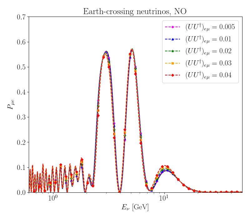
Figure 1: The probability of $\nu_{\mu}\to\nu_{e}$ for neutrino crossing the entire Earth as a function of neutrino energy $E_{\nu}$. We fix $\left(UU^{\dagger}\right)_{ee}=\left(UU^{\dagger}\right)_{\mu\mu}=0.96$, $\left(UU^{\dagger}\right)_{\tau\tau}=1$ while allow $(UU^{\dagger})_{e\mu}$ to vary. As the modulus of $(UU^{\dagger})_{e\mu}$ decreases, the probability approaches that of the standard three-flavor unitarity scenario shown as the solid black line.

We aim to give a more complete theoretical discussion of nonunitarity in neutrino oscillation Antusch et al. (2006); Fernandez-Martinez et al. (2007); Xing (2008); Goswami and Ota (2008); Antusch et al. (2009); Xing (2012); Escrihuela et al. (2015); Parke and Ross-Lonergan (2016); Dutta and Ghoshal (2016); Dutta et al. (2017); Fong et al. (2017); Ge et al. (2017); Blennow et al. (2017); Fong et al. (2019); Martinez-Soler and Minakata (2020a, b); Dutta and Roy (2021); Ellis et al. (2020); Wang and Zhou (2022); Forero et al. (2021); Denton and Gehrlein (2022); Agarwalla et al. (2022); Majumdar et al. (2022); Acero et al. (2022); Argüelles et al. (2023). We start by discussing how apparent nonunitarity can arise in Section II, highlighting two distinct scenarios: high scale nonunitarity scenario where new physics resides beyond the energy scale of neutrino oscillation experiments and low scale nonunitarity scenario where new fermionic states (sterile neutrinos) mix with the SM neutrinos and are accessible in neutrino oscillation experiments. In Section III, we derive analytical solution for neutrino oscillation without assuming unitarity and in Section V, we discuss how the high scale and low scale nonunitarity effects can show up and be distinguished in experiments. Finally we present some concluding remarks in Section VI. While many excellent discussions are there in previous work for e.g. Antusch et al. (2006), we will present some new results. In particular, we will prove a theorem in Section III that if nonunitarity is only diagonal

$$\sum_{i}^{\textrm{accessible}}\mathbf{U}_{\alpha i}\mathbf{U}_{\beta i}^{*} = c_{\alpha}\delta_{\alpha\beta},$$ (2)

with $c_{\alpha}>0$, then neutrino oscillation probability in an arbitrary matter potential is indistinguishable from the unitarity scenario. An important implication is that high scale nonunitarity effects are proportional to the off-diagonal elements of $\mathbf{U}\mathbf{U}^{\dagger}$, in contrast to low scale nonunitarity scenario where the effects can remain. To illustrate this point, in Figure 1, we show the probability of $\nu_{\mu}\to\nu_{e}$ as a function of neutrino energy $E_{\nu}$ in high scale nonunitarity scenario for neutrino passing through the Earth using the public code NuProbe Fong (2022); NuP with a simplified (Preliminary Reference Earth Model) PREM model Dziewonski and Anderson (1981). Denoting $U$ as a $3\times 3$ mixing matrix, we have fixed $(UU^{\dagger})_{ee}=(UU^{\dagger})_{\mu\mu}=0.96$, $(UU^{\dagger})_{\mu\mu}=1$, $(UU^{\dagger})_{e\tau}=(UU^{\dagger})_{\mu\tau}=0$ while varying $(UU^{\dagger})_{e\mu}$ from 0.005 to 0.04 (dashed lines) and the rest of the standard parameters have been fixed to the NO global best fit values from Esteban et al. (2020); NuF . As the modulus of $(UU^{\dagger})_{e\mu}$ decreases, the probability approaches that of the standard three-flavor unitarity scenario (solid black line). For reader interested in experimental probe of nonunitarity scenarios, he or she can jump straight to Section V.

II Models

Here we will focus on models for neutrino oscillation assuming that the center-of-mass energy involved is below the electroweak symmetry breaking $E<v_{\textrm{EW}}\equiv 174$ GeV. We will consider only Majorana mass term for neutrinos though the discussions below are independent of whether we have a Majorana or Dirac mass term. While neutrino oscillation cannot distinguish between strictly Majorana and Dirac mass, it is possible to distinguish them from quasi-Dirac scenario in which both types of mass terms exist while the Majorana mass term is much smaller than the Dirac one Cirelli et al. (2005); de Gouvea et al. (2009); Anamiati et al. (2018, 2019); Fong et al. (2021). We will consider this interesting scenario in a future publication.

II.1 High scale nonunitarity

Assuming that for $E<v_{\textrm{EW}}$, we only have three SM neutrinos ($\nu_{e}$, $\nu_{\mu}$ and $\nu_{\tau}$ are the SM left-handed neutrino flavor states), the general neutrino Lagrangian allowed by the SM electromagnetic gauge symmetry $U(1)_{\textrm{EM}}$ in the charged lepton mass or flavor basis is given by

$${\cal L}_{\nu} = \frac{1}{2}\left(i\overline{\nu_{\alpha}}\not{\partial}D_{\alpha\beta}\nu_{\beta}-\overline{\nu_{\alpha}^{c}}m_{\alpha\beta}\nu_{\beta}+{\rm h.c.}\right)$$ (3)

$$-\left(\frac{g}{2}W_{\mu}^{-}\overline{\ell_{\alpha}}\gamma^{\mu}P_{L}\nu_{\alpha}+\frac{g}{\sqrt{2}\cos\theta_{W}}Z_{\mu}\overline{\nu_{\alpha}}\gamma^{\mu}P_{L}\nu_{\alpha}+{\rm h.c.}\right),$$

where $\alpha,\beta=e,\mu,\tau$ are flavor indices, $D$ is a dimensionless Hermitian matrix while $m$ is a symmetric matrix with mass dimension. In the second line, $g$ is the $SU(2)_{L}$ gauge coupling, $\theta_{W}$ is the Weinberg or weak angle, $P_{L}=\frac{1}{\sqrt{2}}\left(1-\gamma^{5}\right)$ is the left-handed projector, $\left\{\ell_{e},\ell_{\mu},\ell_{\tau}\right\}\equiv\left\{e^{-},\mu^{-},\tau^{-}\right\}$ are the charged leptons and $W^{\mp}$ and $Z$ are the charged and neutral weak bosons, respectively. Without additional light degrees of freedom, only Majorana mass term is possible. Treating the Standard Model as an effective field theory, the neutrino mass and the modified kinetic terms come respectively from dimension-5 Weinberg (1979, 1980) and dimension-6 operators Antusch et al. (2006); Broncano et al. (2003); Antusch and Fischer (2014); Fernandez-Martinez et al. (2016)

$${\cal O}_{5} = \frac{\lambda_{\alpha\beta}}{\Lambda_{5}}\left(\overline{L_{\alpha}^{c}}\epsilon H\right)\left(L_{\beta}^{T}\epsilon H\right),$$ (4)

$${\cal O}_{6} = \frac{\eta_{\alpha\beta}}{\Lambda_{6}^{2}}\left(\overline{L_{\alpha}}\epsilon H^{*}\right)i\not{\partial}\left(L_{\beta}^{T}\epsilon H\right),$$ (5)

where $L_{\alpha}$ and $H$ are the $SU(2)_{L}$ lepton and Higgs doublets, respectively, $\lambda$ and $\eta$ are dimensionless symmetric and Hermitian matrices, respectively, and $\Lambda_{5}$ and $\Lambda_{6}$ are effective scales below which the operators ${\cal O}_{5}$ and ${\cal O}_{6}$ are valid. Implicitly, we have assumed $E\ll\Lambda_{5},\Lambda_{6}$. Not all ultraviolet models which generate ${\cal O}_{5}$ also generate ${\cal O}_{6}$. For instance, type-I and type-III seesaw models generate both ${\cal O}_{5}$ and ${\cal O}_{6}$ while type-II seesaw model only generates ${\cal O}_{5}$.

In order to obtain canonical normalized kinetic term, we can first diagonalize the kinetic term as $D=Y^{\dagger}\hat{D}Y$ where $Y$ is unitary and $\hat{D}$ is real and diagonal. Defining the normalized neutrino fields as $\widetilde{\nu}\equiv\sqrt{\hat{D}}Y\nu$, eq. (3) becomes

$${\cal L}_{\nu} = \frac{1}{2}\left(i\overline{\widetilde{\nu}_{\alpha}}\not{\partial}\widetilde{\nu}_{\alpha}-\overline{\widetilde{\nu}_{\alpha}^{c}}\widetilde{m}_{\alpha\beta}\widetilde{\nu}_{\beta}+{\rm h.c.}\right)$$ (6)

$$-\left[\frac{g}{2}W_{\mu}^{-}\overline{\ell_{\alpha}}\gamma^{\mu}P_{L}\left(Y^{\dagger}\sqrt{\hat{D}}^{-1}\right)_{\alpha\beta}\widetilde{\nu}_{\beta}+\frac{g}{\sqrt{2}\cos\theta_{W}}Z_{\mu}\left(\hat{D}^{-1}\right)_{\alpha\alpha}\overline{\widetilde{\nu}_{\alpha}}\gamma^{\mu}P_{L}\widetilde{\nu}_{\alpha}+{\rm h.c.}\right],$$

where we have defined

$$\widetilde{m} \equiv \sqrt{\hat{D}}^{-1}Y^{*}mY^{\dagger}\sqrt{\hat{D}}^{-1}.$$ (7)

The symmetric mass matrix above can be diagonalized by a unitary matrix $V$ as $\widetilde{m}=V^{*}\hat{m}V^{\dagger}$ where $\hat{m}$ is real and diagonal. Defining the neutrino fields in the mass basis as $\hat{\nu}=V^{\dagger}\widetilde{\nu}$, we have Antusch et al. (2006)

$${\cal L}_{\nu} = \frac{1}{2}\left(i\overline{\hat{\nu}_{i}}\not{\partial}\hat{\nu}_{i}-\overline{\hat{\nu}_{i}^{c}}\hat{m}_{ii}\hat{\nu}_{i}+{\rm h.c.}\right)$$ (8)

$$-\left[\frac{g}{2}W_{\mu}\overline{\ell_{\alpha}}\gamma^{\mu}P_{L}U_{\alpha i}\hat{\nu}_{i}+\frac{g}{\sqrt{2}\cos\theta_{W}}Z_{\mu}\overline{\hat{\nu}_{i}}\left(U^{\dagger}U\right)_{ij}\gamma^{\mu}P_{L}\hat{\nu}_{j}+{\rm h.c.}\right],$$

where we denote $i,j=1,2,3$ to be the indices in mass basis and we have defined

$$U_{\alpha i} \equiv \left(Y^{\dagger}\sqrt{\hat{D}}^{-1}V\right)_{\alpha i}.$$ (9)

Notice that

$$UU^{\dagger} = Y^{\dagger}\hat{D}^{-1}Y,\qquad U^{\dagger}U=V^{\dagger}\hat{D}^{-1}V.$$ (10)

Only if $\hat{D}=I$ is the $3\times 3$ identity matrix, unitarity is restored in which $U^{\dagger}U=UU^{\dagger}=I$. We denote the general case with $UU^{\dagger}\neq I$ and $U^{\dagger}U\neq I$, high scale nonunitarity scenario. Later, we will prove that scenario with $(UU^{\dagger})_{\alpha\beta}=0$ for all $\beta\neq\alpha$ is indistinguishable from unitarity scenario even if $(UU^{\dagger})_{\alpha\alpha}\neq 1$.

II.2 Low scale nonunitarity

Assuming that for $E<v_{\textrm{EW}}$, besides the three SM neutrinos ($\nu_{e}$, $\nu_{\mu}$ and $\nu_{\tau}$), we also have additional neutral fermions fields ($\nu_{s_{1}}$, $\nu_{s_{2}}$,…, $\nu_{s_{N}}$) which do not participate in weak interactions but mix with the SM neutrinos through the mass term. The mixing between the SM and the additional fermions are the Dirac mass term. Here we will focus on mostly Majorana scenario where the Majorana mass term for new fermions is somewhat larger than the Majorana mass for the SM neutrinos as well as the Dirac mass term.

In order to highlight the distinction from the high scale unitarity violation scenario, we further assume that the kinetic terms for all the fermions are canonical. In this case, the $U(1)_{\textrm{EM}}$-invariant neutrino Lagrangian in the charged lepton flavor basis is given by

$${\cal L}_{\nu} = \frac{1}{2}\left(i\overline{\nu_{\tilde{\alpha}}}\not{\partial}\nu_{\tilde{\alpha}}-\overline{\nu_{\tilde{\alpha}}^{c}}m_{\tilde{\alpha}\tilde{\beta}}\nu_{\tilde{\beta}}+{\rm h.c.}\right)$$ (11)

$$-\left(\frac{g}{2}W_{\mu}^{-}\overline{\ell_{\alpha}}\gamma^{\mu}P_{L}\nu_{\alpha}+\frac{g}{\sqrt{2}\cos\theta_{W}}Z_{\mu}\overline{\nu_{\alpha}}\gamma^{\mu}P_{L}\nu_{\alpha}+{\rm h.c.}\right),$$

where $\alpha,\beta,...=e,\mu,\tau$ while $\tilde{\alpha},\tilde{\beta},...=e,\mu,\tau,s_{1},s_{2},...,s_{N}$. The symmetric mass matrix $m$ can be diagonalized by a unitary matrix $\mathbf{U}$ as $m=\mathbf{U}^{*}\hat{m}\mathbf{U}^{\dagger}$ where $\hat{m}$ is real and diagonal. Here and in the following, we use a boldface $\mathbf{U}$ to denote a $\left(3+N\right)\times\left(3+N\right)$ matrix while $U$ is reserved for a $3\times 3$ matrix. Defining the neutrino field in the mass basis as $\hat{\nu}=\mathbf{U}^{\dagger}\nu$, we have

$${\cal L}_{\nu} = \frac{1}{2}\left(i\overline{\hat{\nu}_{i}}\not{\partial}\hat{\nu}_{i}-\overline{\hat{\nu}_{i}^{c}}\hat{m}_{ii}\hat{\nu}_{i}+{\rm h.c.}\right)$$ (12)

$$-\left[\frac{g}{2}W_{\mu}\overline{\ell_{\alpha}}\gamma^{\mu}P_{L}\mathbf{U}_{\alpha i}\hat{\nu}_{i}+\frac{g}{\sqrt{2}\cos\theta_{W}}Z_{\mu}\overline{\hat{\nu}_{i}}\mathbf{U}_{\alpha i}^{*}\gamma^{\mu}P_{L}\mathbf{U}_{\alpha j}\hat{\nu}_{j}+{\rm h.c.}\right],$$

where $i,j,...=1,2,...,3+N$. What distinguish this from the high scale nonunitarity scenario is that the flavor states remain orthogonal since $\mathbf{U}$ is unitary $\mathbf{U}^{\dagger}\mathbf{U}=\mathbf{U}\mathbf{U}^{\dagger}=\mathbf{I}$ where $\mathbf{I}$ is the $\left(3+N\right)\times\left(3+N\right)$ identity matrix.

Strictly speaking, there is no unitarity violation in this case. However, since only the mixing involving the SM neutrinos can be measured, one have

$$\sum_{\alpha=e,\mu,\tau}\mathbf{U}_{\alpha i}\mathbf{U}_{\alpha j}^{*} \neq \delta_{ij}.$$ (13)

Furthermore, if $m_{i>3}\gg\sqrt{\Delta m_{\textrm{atm}}^{2}}$ such that oscillations involving $\nu_{i>3}$ can be averaged out, at leading order in small unitarity violating parameter, the mixing elements involved are those of $i=1,2,3$ which sum to Fong et al. (2017, 2019)

$$\sum_{i=1}^{3}\mathbf{U}_{\alpha i}\mathbf{U}_{\beta i}^{*} \neq \delta_{\alpha\beta}.$$ (14)

We denote this as low scale nonunitarity scenario. If some additional states are not kinematically allowed in the process, one should describe it as in the high scale nonunitarity scenario discussed previously, with possible enlargement of flavor space beyond three dimensions to accommodate additional kinematically accessible states.

III Generic $3+N$ neutrino oscillations

Here we will develop a generic $3+N$ neutrino oscillation framework which can be applied to neutrino oscillation with either unitary or nonunitarity $\mathbf{U}$. In general, the neutrino flavor states $\left|\nu_{\alpha}\right\rangle$ are related to the mass eigenstates $\left|\nu_{i}\right\rangle$ through a matrix $\mathbf{U}$

$$\left|\nu_{\alpha}\right\rangle = \frac{1}{\sqrt{\left(\mathbf{U}\mathbf{U}^{\dagger}\right)_{\alpha\alpha}}}\sum_{i}\mathbf{U}_{\alpha i}^{*}\left|\nu_{i}\right\rangle,$$ (15)

where $\alpha,\beta,...=e,\mu,\tau,s_{1},s_{2},...,s_{N}$ ($\nu_{e}$, $\nu_{\mu}$ and $\nu_{\tau}$ are the SM left-handed neutrino flavor states) and $i,j,...=1,2,...,3+N$. In general, $\mathbf{U}$ does not have to be unitary $\mathbf{U}\mathbf{U}^{\dagger}\neq\mathbf{I}$ and $\mathbf{U}^{\dagger}\mathbf{U}\neq\mathbf{I}$. Since the mass eigenstates are orthogonal $\left\langle\nu_{j}|\nu_{i}\right\rangle=\delta_{ji}$, the flavor states are properly normalized $\left\langle\nu_{\alpha}|\nu_{\alpha}\right\rangle=1$ though they are not necessarily orthogonal but equal to

$$\left\langle\nu_{\beta}|\nu_{\alpha}\right\rangle = \frac{\left(\mathbf{U}\mathbf{U}^{\dagger}\right)_{\beta\alpha}}{\sqrt{\left(\mathbf{U}\mathbf{U}^{\dagger}\right)_{\alpha\alpha}\left(\mathbf{U}\mathbf{U}^{\dagger}\right)_{\beta\beta}}}.$$ (16)

In other words, if there is nonzero overlap between different flavor states and there is a probability of “flavor changing” even at zero distance. In the rest of the article, to avoid expressions crowded with normalization factors, we will define

$$\overline{\mathbf{U}}_{\alpha i} \equiv \frac{\mathbf{U}_{\alpha i}}{\sqrt{\left(\mathbf{U}\mathbf{U}^{\dagger}\right)_{\alpha\alpha}}}.$$ (17)

From eq. (15), we can write the inverse relation

$$\left|\nu_{i}\right\rangle = \sum_{\alpha}\left(\overline{\mathbf{U}}^{*,-1}\right)_{i\alpha}\left|\nu_{\alpha}\right\rangle,$$ (18)

which as a check, verifies the orthogonality of mass eigenstates

$$\left\langle\nu_{j}|\nu_{i}\right\rangle = \sum_{\alpha,\beta}\left(\overline{\mathbf{U}}^{-1}\right)_{j\beta}\left(\overline{\mathbf{U}}^{*,-1}\right)_{i\alpha}\left\langle\nu_{\beta}|\nu_{\alpha}\right\rangle=\left(\overline{\mathbf{U}}^{-1}\overline{\mathbf{U}}\,\overline{\mathbf{U}}^{\dagger}\overline{\mathbf{U}}^{\dagger,-1}\right)_{ji}=\delta_{ji},$$ (19)

where in the second equality, we have used eq. (16).

III.1 Completeness and unitarity

The set of all $\left\{\left|\nu_{i}\right\rangle\right\}$ is complete and from the orthogonality condition, it further satisfies the completeness relation

$$\sum_{i}\left|\nu_{i}\right\rangle\left\langle\nu_{i}\right| = \mathbf{I}.$$ (20)

Inserting the completeness relation above in between $\langle\nu_{\alpha}|\nu_{\alpha}\rangle=1$ implies that the probabilities of a flavor state $\left|\nu_{\alpha}\right\rangle$ being detected as all possible mass eigenstates sum up to unity $\displaystyle\sum_{i}\left|\left\langle\nu_{i}|\nu_{\alpha}\right\rangle\right|^{2}=1$ as required.

For general flavor basis set $\left\{\left|\nu_{\alpha}\right\rangle\right\}$ which is complete but not necessarily orthogonal, it satisfies a modified completeness relation

$$\sum_{\alpha,\beta}\left|\nu_{\alpha}\right\rangle\left[\big{(}\overline{\mathbf{U}}\,\overline{\mathbf{U}}^{\dagger}\big{)}^{-1}\right]_{\alpha\beta}\left\langle\nu_{\beta}\right| = \mathbf{I},$$ (21)

taking into account the possible overlaps between the flavor states. Inserting the relation above into $\langle\nu_{i}|\nu_{i}\rangle=1$, we obtain

$$\sum_{\alpha}\left|\left\langle\nu_{\alpha}|\nu_{i}\right\rangle\right|^{2}+\sum_{\alpha}\sum_{\beta\neq\alpha}\left\langle\nu_{i}|\nu_{\alpha}\right\rangle\left[\big{(}\overline{\mathbf{U}}\,\overline{\mathbf{U}}^{\dagger}\big{)}^{-1}\right]_{\alpha\beta}\left\langle\nu_{\beta}|\nu_{i}\right\rangle = 1.$$ (22)

For nonorthogonal flavor states, we can no longer interpret the first term as the sum of the probabilities of a mass eigenstate $\nu_{i}$ to be measured in all possible flavor eigenstates $\nu_{\alpha}$. In this case, the correct probability of detecting a flavor state $\nu_{\alpha}$ from $\nu_{i}$ has to include the contributions from other flavor states as follows

$$P_{\alpha i}=\left|\left\langle\nu_{\alpha}|\nu_{i}\right\rangle\right|^{2}+\sum_{\beta\neq\alpha}\left\langle\nu_{i}|\nu_{\alpha}\right\rangle\left[\big{(}\overline{\mathbf{U}}\,\overline{\mathbf{U}}^{\dagger}\big{)}^{-1}\right]_{\alpha\beta}\left\langle\nu_{\beta}|\nu_{i}\right\rangle,$$ (23)

and from eq. (22), summing over $\alpha$ gives unity as required. With orthogonal flavor states $\left[\big{(}\overline{\mathbf{U}}\,\overline{\mathbf{U}}^{\dagger}\big{)}^{-1}\right]_{\alpha\beta}=\delta_{\alpha\beta}$, one recover the standard result.

Since the flavor state space is complete, one also expect the oscillation probability of $\nu_{\alpha}$ to all possible final flavor states to sum up to one

$$\sum_{\beta}P_{\beta\alpha}=1.$$ (24)

However, considering possible nonorthogonal flavor states, the probability will be modified from the usual expression $P_{\beta\alpha}=|\left\langle\nu_{\beta}|\nu_{\alpha}\right\rangle|^{2}$. In Section IV, we will discuss the probability operator which gives rise to probability that preserves unitarity as in eq. (24).

III.2 Evolution of a flavor state

Starting from an initial state $\left|\nu_{\alpha}\left(0\right)\right\rangle=\left|\nu_{\alpha}\right\rangle$, the time-evolved state $\left|\nu_{\alpha}\left(t\right)\right\rangle$ is described by the Schrödinger equation

$$i\frac{d}{dt}\left|\nu_{\alpha}\left(t\right)\right\rangle = {\cal H}\left|\nu_{\alpha}\left(t\right)\right\rangle,$$ (25)

where the Hamiltonian is ${\cal H}={\cal H}_{0}+{\cal H}_{I}$ with ${\cal H}_{0}$ the free Hamiltonian

$${\cal H}_{0}\left|\nu_{i}\right\rangle = E_{i}\left|\nu_{i}\right\rangle,\;\;\;\;\;E_{i}=\sqrt{\vec{p}_{i}^{\;\leavevmode\nobreak\ 2}+m_{i}^{2}},$$ (26)

and ${\cal H}_{I}$ the interaction Hamiltonian with matrix elements

$$\left\langle\nu_{\beta}\right|{\cal H}_{I}\left|\nu_{\alpha}\right\rangle = V_{\beta\alpha}.$$ (27)

Since ${\cal H}_{I}^{\dagger}={\cal H}_{I}$, we have $V_{\beta\alpha}^{*}=V_{\alpha\beta}$.

Assuming relativistic neutrinos, we trade $t=x$ and the amplitude of the transition $\nu_{\alpha}\to\nu_{\beta}$ at distance $x$ is then given by $S_{\beta\alpha}\left(x\right)\equiv\left\langle\nu_{\beta}|\nu_{\alpha}\left(x\right)\right\rangle$. From eq. (25), we can write the evolution equation of $S_{\beta\alpha}\left(x\right)$ as

$$i\frac{d}{dx}S_{\beta\alpha}\left(x\right) = \left\langle\nu_{\beta}\right|{\cal H}_{0}+{\cal H}_{I}\left|\nu_{\alpha}\left(t\right)\right\rangle$$ (28)

$$= \sum_{i}\left\langle\nu_{\beta}\right|{\cal H}_{0}+{\cal H}_{I}\left|\nu_{i}\right\rangle\left\langle\nu_{i}|\nu_{\alpha}\left(t\right)\right\rangle$$

$$= \sum_{\eta}\left\{\sum_{i}\overline{\mathbf{U}}_{\beta i}E_{i}\big{(}\overline{\mathbf{U}}^{-1}\big{)}_{i\eta}+\sum_{\gamma}V_{\beta\gamma}\left[\big{(}\overline{\mathbf{U}}\,\overline{\mathbf{U}}^{\dagger}\big{)}^{-1}\right]_{\gamma\eta}\right\}S_{\eta\alpha}\left(x\right),$$

where in the second equality, we have inserted the completeness relation eq. (20) and in the last equality, we have used eqs. (26), (27), (18) and (16). Considering relativistic neutrinos $E\gg m_{i}$ and expanding $E_{i}\simeq E+\frac{m_{i}^{2}}{2E}$, we obtain, in matrix notation

$$i\frac{dS\left(x\right)}{dx} = \left[\overline{\mathbf{U}}\Delta\overline{\mathbf{U}}^{-1}+V\big{(}\overline{\mathbf{U}}\,\overline{\mathbf{U}}^{\dagger}\big{)}^{-1}\right]S\left(x\right),$$ (29)

where

$$\Delta \equiv \frac{1}{2E}\textrm{diag}\left(m_{1}^{2},m_{2}^{2},...,m_{3+N}^{2}\right)=\textrm{diag}\left(\Delta_{1},\Delta_{2},...,\Delta_{3+N}\right).$$ (30)

We have dropped the constant $E$ which is an overall phase in $S(x)$ and not observable.

III.3 Vacuum mass basis

From eq. (29), the Hamiltonian in the flavor basis given by

$$H \equiv \overline{\mathbf{U}}\Delta\overline{\mathbf{U}}^{-1}+V\big{(}\overline{\mathbf{U}}\,\overline{\mathbf{U}}^{\dagger}\big{)}^{-1},$$ (31)

is not Hermitian $H^{\dagger}\neq H$ nor normal $H^{\dagger}H\neq HH^{\dagger}$. In the following, we will prove that they can be diagonalized with real eigenvalues. Furthermore, we will argue that despite the apparent non-Hermitian Hamiltonian, unitarity is actually preserved.

Let us change the Hamiltonian to the vacuum mass basis in which the free Hamiltonian is diagonal

$$\widetilde{H} \equiv \overline{\mathbf{U}}^{-1}H\overline{\mathbf{U}}=\Delta+\overline{\mathbf{U}}^{-1}V\overline{\mathbf{U}}^{\dagger,-1}.$$ (32)

Notice that eq. (32) is Hermitian $\widetilde{H}^{\dagger}=\widetilde{H}$. Assuming $V=V^{\dagger}$ is constant in the interval of interest $0\leq x<x_{1}$, we can diagonalize the $\widetilde{H}$ with a unitary matrix $X$

$$\widetilde{H} = X\hat{H}X^{\dagger},$$ (33)

where $X$ is unitary and $\hat{H}=\textrm{diag}\left(\lambda_{1},\lambda_{2},...,\lambda_{3+N}\right)$ is diagonal and real. Since eqs. (31) and (32) are related by similar transformation, they have the same eigenvalues $\widetilde{H}X=X\hat{H}\implies H\overline{\mathbf{U}}X=\overline{\mathbf{U}}X\hat{H}$ and hence we can also write

$$H = \overline{\mathbf{U}}X\hat{H}\left(\overline{\mathbf{U}}X\right)^{-1},$$ (34)

where the nonnormal $H$ is diagonalized by a nonunitary $\overline{\mathbf{U}}X$. We see explicitly that despite the Hamiltonian in flavor basis $H$ appears to be non-Hermitian, the eigenvalues remain real while the source of non Hermicity comes from nonunitary transformation matrix $\mathbf{U}$. Although $\overline{\mathbf{U}}X$ is nonunitary, one can formally solve for $\left(\overline{\mathbf{U}}X\right)_{\alpha i}\left(\overline{\mathbf{U}}X\right)_{i\beta}^{-1}$ in terms of eigenvalues and Hamiltonian elements using the same method as in refs. Yasuda (2007); Fong (2022). Nevertheless, as we will see in the next subsection, the combination which appears in neutrino oscillation probability is not $\left(\overline{\mathbf{U}}X\right)_{\alpha i}\left(\overline{\mathbf{U}}X\right)_{i\beta}^{-1}$ but $\left(\overline{\mathbf{U}}X\right)_{\alpha i}\left(\overline{\mathbf{U}}X\right)_{i\beta}^{\dagger}$ and hence we will solve for $X_{ik}X_{jk}^{*}$ instead.

Now let us pause to ask a valid question: do we expect unitarity to be violated? In the vacuum mass basis, since the Hamiltonian (32) is Hermitian, unitarity should be preserved under time evolution. By doing a similarity transformation with non-Hermitian $\overline{\mathbf{U}}$ back to the flavor basis Hamitonian (31) appears to be non-Hermitian but this is just an apparent feature. As long as a non-Hermitian Hamiltonian can be transformed to a Hermitian Hamiltonian by similarity transformation, unitarity is preserved. This is also expected from the outset since the flavor space is complete.

As shown in refs. Yasuda (2007); Fong (2022), by raising eq. (33) to the power of $1,2,...,2+N$ and taking into account the unitarity relation $XX^{\dagger}=\mathbf{I}$, one can form a set of $3+N$ linearly independent equations for $X_{ik}X_{jk}^{*}$ where the coefficients form a Vandermonde matrix which can be inverted to give Fong (2022) (see also the pioneering work of Kimura, Takamura and Yokomakura who applied similar method for 3-flavor scenario Kimura et al. (2002a, b))

$$X_{ik}X_{jk}^{*} = \frac{{\displaystyle\sum_{p=0}^{2+N}}\left(-1\right)^{p}(\widetilde{H}^{p})_{ij}c_{2+N-p,k}}{Z_{k}},$$ (35)

where we have defined

$$Z_{k} \equiv \prod_{p\neq k}\left(\lambda_{p}-\lambda_{k}\right),$$ (36)

$$c_{p,k} \equiv \sum_{\left\{q\neq r\neq...\right\}\neq k}\underbrace{\lambda_{q}\lambda_{r}...}_{p},$$ (37)

with $[\tilde{H}^{0}]_{ij}=\delta_{ij}$ and $c_{0,k}=1$. The sum in $c_{p,k}$ is over all possible unordered combinations of $p$ distinct eigenvalues $\lambda_{q}\lambda_{r}...$ where none of them is equal to $\lambda_{k}$ and hence with $3+N$ neutrino flavors, $c_{p,k}$ has $\left(\begin{smallmatrix}2+N\\ p\end{smallmatrix}\right)=\frac{\left(2+N\right)!}{p!\left(2+N-p\right)!}$ terms in the sum. As shown in ref. Abdullahi and Parke (2022), the numerator of eq. (35) can be written in mathematically equivalent form in terms of elements of the adjugate of $\lambda_{k}I-\widetilde{H}$ i.e. $[\textrm{Adj}(\lambda_{k}I-\widetilde{H})]_{ij}$ and can be equally fast in numerical evaluation using the Le Verrier-Faddeev algorithm.

III.4 Oscillation probability

There is one subtle but crucial point regarding $\widetilde{S}$ in the vacuum mass basis which satisfies

$$i\frac{d\widetilde{S}\left(x\right)}{dx} = \widetilde{H}\widetilde{S}\left(x\right),$$ (38)

and the solution is given by

$$\widetilde{S}\left(x\right) = Xe^{-i\hat{H}x}X^{\dagger}.$$ (39)

How do we relate $\widetilde{S}\left(x\right)$ of the vacuum mass basis and $S\left(x\right)$ in the flavor basis? Fixing the initial conditions $\widetilde{S}\left(0\right)=\mathbf{I}$ and $S\left(0\right)=\overline{\mathbf{U}}\,\overline{\mathbf{U}}^{\dagger}$ which follow from the orthogonality of mass eigenstates and the nonorthogonality of flavor eigenstates eq. (16), respectively, we have

$$\widetilde{S}\left(x\right) \equiv \overline{\mathbf{U}}^{-1}S\left(x\right)\overline{\mathbf{U}}^{\dagger,-1}.$$ (40)

Hence we can write

$$S_{\beta\alpha}\left(x\right) = \left[\overline{\mathbf{U}}Xe^{-i\hat{H}x}\left(\overline{\mathbf{U}}X\right)^{\dagger}\right]_{\beta\alpha}=\sum_{i,j,k}\overline{\mathbf{U}}_{\beta i}\overline{\mathbf{U}}_{\alpha j}^{*}X_{ik}X_{jk}^{*}e^{-i\lambda_{k}x},$$ (41)

which has exactly the same form as the unitarity case despite that $\overline{\mathbf{U}}$ does not have to be unitary.

The probability of an initial state $\left|\nu_{\alpha}\right\rangle$ being detected as $\left|\nu_{\beta}\right\rangle$ at distance $0<x<x_{1}$ (where $V(x)$ is constant) is

$$P_{\beta\alpha}\left(x\right) = \sum_{\xi,\lambda}S_{\alpha\xi}(x)(\hat{P}_{\beta})_{\xi\lambda}S_{\lambda\alpha}(x).$$ (42)

The appearance of $(\hat{P}_{\beta})_{\xi\lambda}$ takes into account possible nonorthogonality of flavor states. Since this is a nontrivial result with subtleties, the discussion of $(\hat{P}_{\beta})_{\xi\lambda}$ will be deferred to Section IV. For the moment, note that summing over $\beta$, we have

$$\sum_{\beta}(\hat{P}_{\beta})_{\xi\lambda}=\left[\big{(}\overline{\mathbf{U}}\,\overline{\mathbf{U}}^{\dagger}\big{)}^{-1}\right]_{\xi\lambda}.$$ (43)

Together with eq. (21), this guarantees that $\sum_{\beta}P_{\beta\alpha}(x)=1$. For orthogonal flavor states, we have

$$(\hat{P}_{\beta})_{\xi\lambda}=\delta_{\xi\beta}\delta_{\lambda\beta},$$ (44)

which gives the standard expression $P_{\beta\alpha}\left(x\right)=\left|S_{\beta\alpha}\left(x\right)\right|^{2}$. Using eq. (44) for nonorthogonal flavor states will lead inconsistent result which violates unitarity $\sum_{\beta}P_{\alpha\beta}\neq 1$. By substituting eq. (44) into eq. (42), it is sufficient to show this violation at zero distance $x=0$ with $X_{ij}=\delta_{ij}$ in which we obtain

$$P_{\beta\alpha}\left(0\right) = (\overline{\mathbf{U}}\,\overline{\mathbf{U}}^{\dagger})_{\alpha\beta}(\overline{\mathbf{U}}\,\overline{\mathbf{U}}^{\dagger})_{\beta\alpha}=|(\overline{\mathbf{U}}\,\overline{\mathbf{U}}^{\dagger})_{\beta\alpha}|^{2},$$ (45)

which implies $\sum_{\beta}P_{\beta\alpha}(0)>1$ if the flavor states are nonorthogonal since $(\overline{\mathbf{U}}\,\overline{\mathbf{U}}^{\dagger})_{\alpha\alpha}=1$.

One can generalize the solution in eq. (41) to the case when $V$ is $x$-dependent by splitting $x$ into intervals small enough that $V\left(x\right)$ is approximately constant. Considering $0=x_{0}<x_{1}<x_{2}<...$ where $V\left(x\right)$ is equal to constant $V_{a}$ for each interval $x_{a-1}<x<x_{a}$, we obtain

$$S\left(x\right) = T\prod_{a=1}\big{(}\overline{\mathbf{U}}\,\overline{\mathbf{U}}^{\dagger}\big{)}^{-1}S^{\left(a\right)}\left(x\right),$$ (46)

where we have defined

$$S^{\left(a\right)}\left(x\right) \equiv \left(\overline{\mathbf{U}}X^{\left(a\right)}\right)e^{-i\hat{H}^{\left(a\right)}x^{\left(a\right)}}\left(\overline{\mathbf{U}}X^{\left(a\right)}\right)^{\dagger},$$ (47)

$$x^{\left(a\right)} \equiv \left[\left(x-x_{a-1}\right)\theta\left(x_{a}-x\right)+\left(x_{a}-x_{a-1}\right)\theta\left(x-x_{a}\right)\right]\theta\left(x-x_{a-1}\right),$$ (48)

with $\theta\left(x\geq 0\right)=1$, $\theta\left(x<0\right)=0$ and $T$ denotes the space ordering of the matrix multiplication such that the $a$ term is always to the left of $a-1$ term. The factor $\big{(}\overline{\mathbf{U}}\,\overline{\mathbf{U}}^{\dagger}\big{)}^{-1}$ appears due to eq. (21) in order to take into account possible nonorthogonality of flavor states. Furthermore, $\hat{H}^{\left(a\right)}=\textrm{diag}\left(\lambda_{1}^{\left(a\right)},\lambda_{2}^{\left(a\right)},...,\lambda_{3+N}^{\left(a\right)}\right)$ and $X^{\left(a\right)}$ denote respectively the matrix of eigenvalues and unitary matrix which diagonalizes $\widetilde{H}$ as $\widetilde{H}^{\left(a\right)}=X^{\left(a\right)\dagger}\hat{H}^{\left(a\right)}X^{\left(a\right)}$ in the interval $x_{a-1}<x<x_{a}$. The neutrino oscillation probability can be calculated by substituting eq. (46) into eq. (42).

We will end this section by proving the following theorem.

Theorem.

If $\left(\mathbf{U}\mathbf{U}^{\dagger}\right)_{\alpha\alpha}\neq 1$ and $\left(\mathbf{U}\mathbf{U}^{\dagger}\right)_{\alpha\beta}=0$ for all $\alpha\neq\beta$, then the neutrino oscillation probability in an arbitrary matter potential is indistinguishable from the unitarity scenario.

The proof is as follows

$$\sum_{i}\overline{\mathbf{U}}_{\beta i}\overline{\mathbf{U}}_{\alpha i}^{*} = \frac{1}{\sqrt{\left(\mathbf{U}\mathbf{U}^{\dagger}\right)_{\alpha\alpha}\left(\mathbf{U}\mathbf{U}^{\dagger}\right)_{\beta\beta}}}\sum_{i}\mathbf{U}_{\beta i}\mathbf{U}_{\alpha i}^{*}=\frac{\left(\mathbf{U}\mathbf{U}^{\dagger}\right)_{\alpha\alpha}\delta_{\alpha\beta}}{\sqrt{\left(\mathbf{U}\mathbf{U}^{\dagger}\right)_{\alpha\alpha}\left(\mathbf{U}\mathbf{U}^{\dagger}\right)_{\beta\beta}}}=\delta_{\alpha\beta}.$$ (49)

From the above, it follows that $\left(\overline{\mathbf{U}}\,\overline{\mathbf{U}}^{\dagger}\right)^{-1}=\mathbf{I}\implies\overline{\mathbf{U}}^{\dagger,-1}\overline{\mathbf{U}}^{-1}=\mathbf{I}\implies\overline{\mathbf{U}}^{\dagger}\overline{\mathbf{U}}=\mathbf{I}$ and hence $\overline{\mathbf{U}}$ is unitary. With unitary $\overline{\mathbf{U}}$, the Hamiltonians in the vacuum mass basis in eq. (32) reduces and coincides with the unitarity one and hence the solution in eq. (47) will coincide with the unitarity scenario as well. This result holds for an arbitrary matter potential $V\left(x\right)$ since one can always construct the full solution as in (46). Finally, we will also recover eq. (44) as will be discussed in Section IV. Let us denote this scenario as the hidden nonunitarity scenario.

III.5 Identities

The combination that appears in the oscillation amplitude in the flavor basis (41) is

$$\mathbf{\widetilde{U}}_{\beta k}\mathbf{\widetilde{U}}_{\alpha k}^{*} \equiv \sum_{i,j}\overline{\mathbf{U}}_{\beta i}\overline{\mathbf{U}}_{\alpha j}^{*}X_{ik}X_{jk}^{*}.$$ (50)

Substituting eq. (35) into the equation above, we obtain

$$\mathbf{\widetilde{U}}_{\beta k}\mathbf{\widetilde{U}}_{\alpha k}^{*} = \frac{{\displaystyle\sum_{p=0}^{2+N}}\left(-1\right)^{p}\left(\overline{H}^{p}\right)_{\beta\alpha}c_{2+N-p,k}}{Z_{k}},$$ (51)

where we have defined

$$\overline{H} \equiv \overline{\mathbf{U}}\widetilde{H}\overline{\mathbf{U}}^{\dagger}=H\overline{\mathbf{U}}\,\overline{\mathbf{U}}^{\dagger}=\overline{\mathbf{U}}\Delta\overline{\mathbf{U}}^{\dagger}+V,$$ (52)

and we have used eq. (32) and eq. (31) to arrive at the last equality. It is important to note that $\overline{H}$ is not equal to the Hamiltonian in the flavor basis $H$ but they only coincide with each other if $\overline{\mathbf{U}}$ is unitary. Furthermore, $\overline{H}$, not being related to $\widetilde{H}$ and $H$ by similarity transformation, does not have to have the same eigenvalues as $\widetilde{H}$ and $H$.

Under trace transformation $H\to H+c\,\mathbf{I}$ with $c$ any real constant or phase transformation $H\to\Phi H\Phi^{\dagger}$ with $\Phi=\textrm{diag}\left(e^{i\phi_{1}},e^{i\phi_{2}},...\right)$, the probabilities (measureables) (42) remain invariant. By observing that the following trace and phase transformation invariant combinations Harrison and Scott (2002)

$$I_{\alpha\beta} = \textrm{Im}\left[\left(H^{2}\right)_{\alpha\beta}H_{\alpha\beta}^{*}\right],$$ (53)

$$R_{\alpha\beta} = \left|H_{\alpha\beta}\right|^{2},\quad\alpha\neq\beta,$$ (54)

should be independent of matter potential if the matter potential is diagonal in the flavor basis, several matter invariant identities can be derived. With unitary $\overline{\mathbf{U}}$, the first one results in the Naumov-Harrison-Scott (NHS) identity Naumov (1992); Harrison and Scott (2002) or their generalized versions Abdullahi and Parke (2022) while the second one results in further matter-invariant identities Harrison and Scott (2002); Abdullahi and Parke (2022). In the nonunitarity scenario, this is no longer true since the matter potential in the flavor basis (31) is no longer diagonal but given by $V\left(\overline{\mathbf{U}}\,\overline{\mathbf{U}}^{\dagger}\right)^{-1}$. Incidentally, this also shows that once we have nondiagonal NonStandard neutrino Interaction (NSI), eqs. (53) and (54) are no longer invariant under matter potential Fong (2022); Abdullahi and Parke (2022). As shown in ref. Fong (2022), NSI is still distinct from nonunitarity scenario since the latter further breaks the unitarity relations that we will discuss next.

Let us define the Jarlskog combinations by taking the imaginary part of the combination above Jarlskog (1985)

$$J_{\beta\alpha}^{jk} \equiv \textrm{Im}\left(\mathbf{\widetilde{U}}_{\beta j}\mathbf{\widetilde{U}}_{\alpha j}^{*}\mathbf{\widetilde{U}}_{\beta k}^{*}\mathbf{\widetilde{U}}_{\alpha k}\right).$$ (55)

If $\widetilde{\mathbf{U}}$ is unitary, one must have

$$\sum_{k}J_{\beta\alpha}^{jk} = \sum_{k}\textrm{Im}\left(\mathbf{\widetilde{U}}_{\beta j}\mathbf{\widetilde{U}}_{\alpha j}^{*}\mathbf{\widetilde{U}}_{\beta k}^{*}\mathbf{\widetilde{U}}_{\alpha k}\right)=\textrm{Im}\left(\mathbf{\widetilde{U}}_{\beta j}\mathbf{\widetilde{U}}_{\beta j}^{*}\right)=0.$$ (56)

Let us look at the modification due to nonunitarity. Since all the terms with $p=q$ are real and we are only left with terms of $p\neq q$

$$J_{\beta\alpha}^{jk} = {\displaystyle\sum_{p\neq q;0\leq p<q}^{2+N}}\left(-1\right)^{p+q}\frac{c_{2+N-p,j}c_{2+N-q,k}-c_{2+N-q,j}c_{2+N-p,k}}{Z_{j}Z_{k}}\textrm{Im}\left[\left(\overline{H}^{p}\right)_{\beta\alpha}\left(\overline{H}^{q}\right)_{\beta\alpha}^{*}\right],$$ (57)

where there is no sum over $j$ and $k$ on the right and we have used $\textrm{Im}z=-\textrm{Im}z^{*}$. Summing over $k$ and making use of

$$\sum_{k=1}^{3+N}\frac{c_{2+N-p,k}}{Z_{k}} = \begin{cases}0&p>0\\ 1&p=0\end{cases},$$ (58)

we arrive at

$$\sum_{k}J_{\beta\alpha}^{jk} = {\displaystyle\sum_{q=1}^{2+N}}\left(-1\right)^{q+1}\frac{c_{2+N-q,j}}{Z_{j}}\textrm{Im}\left[\big{(}\overline{\mathbf{U}}\,\overline{\mathbf{U}}^{\dagger}\big{)}_{\beta\alpha}\left(\overline{H}^{q}\right)_{\beta\alpha}^{*}\right],$$ (59)

where we have used $\overline{H}^{0}=\overline{\mathbf{U}}\,\overline{\mathbf{U}}^{\dagger}$. For unitary $\overline{\mathbf{U}}\implies\big{(}\overline{\mathbf{U}}\,\overline{\mathbf{U}}^{\dagger}\big{)}_{\beta\alpha}=\delta_{\beta\alpha}$ and since $\overline{H}^{q}$ is Hermitian, the diagonal elements are real and we recover eq. (56). This is consistent with the theorem we have proven and indeed, if $\left(\mathbf{U}\mathbf{U}^{\dagger}\right)_{\alpha\beta}=0$ for all $\alpha\neq\beta$, the right hand side of eq. (59) vanishes. In the vacuum, $\overline{H}^{q}=\big{(}\overline{\mathbf{U}}\Delta\overline{\mathbf{U}}^{\dagger}\big{)}^{q}$ and one recover

$$\sum_{k}J_{\beta\alpha}^{jk} = -\textrm{Im}\left[\big{(}\overline{\mathbf{U}}\,\overline{\mathbf{U}}^{\dagger}\big{)}_{\beta\alpha}\overline{\mathbf{U}}_{\alpha j}\overline{\mathbf{U}}_{\beta j}^{*}\right],$$ (60)

as can also be derived directly from eq. (55). So by measuring these relations above, we can uncover unitarity violation in the matter (59) or in the vacuum (60).

IV Oscillation probability for nonorthogonal flavor states

Probability is not an observable in quantum mechanics and there is no associated Hermitian operator. Typically, to calculate probability of a state $\left|\nu_{\alpha}\right\rangle$ being found in $\left|\nu_{\beta}\right\rangle$, one insert the projection operator $\left|\nu_{\beta}\right\rangle\left\langle\nu_{\beta}\right|$ in between $\left\langle\nu_{\alpha}|\nu_{\alpha}\right\rangle$ and obtain the probability $P_{\beta\alpha}=|\left\langle\nu_{\beta}|\nu_{\alpha}\right\rangle|^{2}$ which is the Born rule.

When the complete set of states $\left\{\left|\nu_{\alpha}\right\rangle\right\}$ are not orthogonal, from eq. (21), the projection operator becomes

$$P_{\alpha} \equiv \sum_{\beta}\left|\nu_{\alpha}\right\rangle\left[\big{(}\overline{\mathbf{U}}\,\overline{\mathbf{U}}^{\dagger}\big{)}^{-1}\right]_{\alpha\beta}\left\langle\nu_{\beta}\right|,$$ (61)

which satisfies $P_{\alpha}^{2}=P_{\alpha}$ and $\sum_{\alpha}P_{\alpha}=\mathbf{I}$. Inserting this projection operator in between $\left\langle\nu_{\alpha}|\nu_{\alpha}\right\rangle$, we obtain

$$\left\langle\nu_{\alpha}|P_{\beta}|\nu_{\alpha}\right\rangle = \left|\left\langle\nu_{\beta}|\nu_{\alpha}\right\rangle\right|^{2}+\sum_{\gamma\neq\beta}\left\langle\nu_{\alpha}|\nu_{\beta}\right\rangle\left[\big{(}\overline{\mathbf{U}}\,\overline{\mathbf{U}}^{\dagger}\big{)}^{-1}\right]_{\beta\gamma}\left\langle\nu_{\gamma}|\nu_{\alpha}\right\rangle.$$ (62)

Notice that the second term is in general complex and hence the quantity above cannot be interpreted as a probability. Besides being real and positive, one has to make sure that the probabilities of finding $\left|\nu_{\alpha}\right\rangle$ in all possible $\left|\nu_{\beta}\right\rangle$ sum up to unity. According to the theorem in the last section, if $\left(\mathbf{U}\mathbf{U}^{\dagger}\right)_{\alpha\beta}=0$ for all $\alpha\neq\beta$, eq. (61) becomes the standard projector and we recover eq. (44).

Nonorthogonal basis states are commonplace in quantum chemistry Mulliken (1955); Roby (1974); Leon and Neshyba (1988); Manning and De Leon (1990); Artacho and Miláns del Bosch (1991); Soriano and Palacios (2014); Artacho and O'Regan (2017), for example, to express molecular orbitals as linear combinations of atomic orbitals which are in general not orthogonal. In particle physics, nonorthogonal basis states can arise due to new physics as in our consideration of high scale nonunitarity scenario. In ref. Leon and Neshyba (1988); Manning and De Leon (1990), the theory of projected probabilities on nonorthogonal states are developed and for two and three states system, the probability operators have closed form. We will write down the results here and defer the details to Appendix B.

Before moving to the realistic three-flavor scenario, we will first show the two-flavor result since they are simpler and illustrative. Denoting ${\cal N}_{\alpha\beta}\equiv(\overline{U}\,\overline{U}^{\dagger})_{\alpha\beta}$ and let us choose the two flavors as $e,\mu$ (it can also be $e,\tau$ or $\mu,\tau$), $(\hat{P}_{\alpha})_{\xi\lambda}$ in eq. (42) is given by

$$(\hat{P}_{\alpha})_{\xi\lambda} = \begin{cases}\displaystyle{1+\frac{\left|{\cal N}_{e\mu}\right|^{4}}{1-\left|{\cal N}_{e\mu}\right|^{4}}},&\xi=\lambda=\alpha\\ {\displaystyle\frac{\left|{\cal N}_{e\mu}\right|^{2}}{1-\left|{\cal N}_{e\mu}\right|^{4}}},&\xi=\lambda\neq\alpha\\ \displaystyle{-\frac{1}{2}\frac{{\cal N}_{\xi\lambda}}{1-\left|{\cal N}_{e\mu}\right|^{2}}},&\xi\neq\lambda\;\textrm{and}\;\xi=\alpha\;\textrm{or}\;\lambda=\alpha\end{cases}.$$ (63)

In the case where off-diagonal elements of ${\cal N}$ are zero, we recover eq. (44). It is clear that the deviation from the standard unitarity scenario depends on the off-diagonal elements. From eq. (42), let us write down the oscillation probabilities explicitly

$$P_{ee} = \left|S_{ee}\right|^{2}+\frac{\left|{\cal N}_{e\mu}\right|^{4}\left|S_{ee}\right|^{2}+\left|{\cal N}_{e\mu}\right|^{2}\left|S_{e\mu}\right|^{2}}{1-\left|{\cal N}_{e\mu}\right|^{4}}-\frac{\textrm{Re}\left(S_{ee}{\cal N}_{e\mu}S_{\mu e}\right)}{1-\left|{\cal N}_{e\mu}\right|^{2}},$$ (64)

$$P_{\mu e} = \left|S_{e\mu}\right|^{2}+\frac{\left|{\cal N}_{e\mu}\right|^{4}\left|S_{e\mu}\right|^{2}+\left|{\cal N}_{e\mu}\right|^{2}\left|S_{ee}\right|^{2}}{1-\left|{\cal N}_{e\mu}\right|^{4}}-\frac{\textrm{Re}\left(S_{ee}{\cal N}_{e\mu}S_{\mu e}\right)}{1-\left|{\cal N}_{e\mu}\right|^{2}},$$ (65)

$$P_{e\mu} = \left|S_{e\mu}\right|^{2}+\frac{\left|{\cal N}_{e\mu}\right|^{4}\left|S_{e\mu}\right|^{2}+\left|{\cal N}_{e\mu}\right|^{2}\left|S_{\mu\mu}\right|^{2}}{1-\left|{\cal N}_{e\mu}\right|^{4}}-\frac{\textrm{Re}\left(S_{\mu\mu}{\cal N}_{\mu e}S_{e\mu}\right)}{1-\left|{\cal N}_{e\mu}\right|^{2}},$$ (66)

$$P_{\mu\mu} = \left|S_{\mu\mu}\right|^{2}+\frac{\left|{\cal N}_{e\mu}\right|^{4}\left|S_{\mu\mu}\right|^{2}+\left|{\cal N}_{e\mu}\right|^{2}\left|S_{e\mu}\right|^{2}}{1-\left|{\cal N}_{e\mu}\right|^{4}}-\frac{\textrm{Re}\left(S_{\mu\mu}{\cal N}_{\mu e}S_{e\mu}\right)}{1-\left|{\cal N}_{e\mu}\right|^{2}}.$$ (67)

The first terms have the standard form, while the additional terms are required to ensure unitarity. Notice that the expressions above hold for any matter potential (including vacuum) since the dynamics is contained in the amplitude $S$ obtained by solving the Schrödinger equation in Section III.2. We can verify explicitly that unitarity is preserved

$$P_{ee}+P_{\mu e} = \frac{\left|S_{ee}\right|^{2}+\left|S_{e\mu}\right|^{2}-2\textrm{Re}\left(S_{ee}{\cal N}_{e\mu}S_{\mu e}\right)}{1-\left|{\cal N}_{e\mu}\right|^{2}}=\sum_{\alpha,\beta}\left\langle\nu_{e}|\nu_{\alpha}\right\rangle\left({\cal N}^{-1}\right)_{\alpha\beta}\left\langle\nu_{\beta}|\nu_{e}\right\rangle=1,$$ (68)

$$P_{e\mu}+P_{\mu\mu} = \frac{\left|S_{\mu\mu}\right|^{2}+\left|S_{e\mu}\right|^{2}-2\textrm{Re}\left(S_{\mu\mu}{\cal N}_{\mu e}S_{e\mu}\right)}{1-\left|{\cal N}_{e\mu}\right|^{2}}=\sum_{\alpha,\beta}\left\langle\nu_{\mu}|\nu_{\alpha}\right\rangle\left({\cal N}^{-1}\right)_{\alpha\beta}\left\langle\nu_{\beta}|\nu_{\mu}\right\rangle=1,$$ (69)

where we have used eq. (21) in the third equalities.

For three flavors scenario $\alpha,\beta,...=\{e,\mu,\tau\}$, ${\cal N}$ is a $3\times 3$ matrix with diagonal elements all equal to one. We will next define ${\cal N}_{\alpha}$ as a $2\times 2$ submatrix formed from the matrix ${\cal N}$ excluding the row and column involving $\nu_{\alpha}$ state. The result is

$$(\hat{P}_{\alpha})_{\xi\lambda} = \frac{1}{3}\left[(E_{\alpha})_{\xi\lambda}+\sum_{\beta\neq\alpha}(F_{\alpha\beta})_{\xi\lambda}\right],$$ (70)

with

$$\left(E_{\alpha}\right)_{\xi\lambda} = \begin{cases}{\displaystyle 1+\frac{X_{\alpha}^{2}}{1-X_{\alpha}^{2}}},&\xi=\lambda=\alpha\\ {\displaystyle\frac{\left|{\cal N}_{\alpha\xi}-{\cal N}_{\alpha\gamma\xi}\right|^{2}}{\left(\det{\cal N}_{\alpha}\right)^{2}\left(1-X_{\alpha}^{2}\right)},\;\gamma\neq\left\{\alpha,\xi\right\}},&\xi=\lambda\neq\alpha\\ {\displaystyle-\frac{1}{2}\frac{{\cal N}_{\xi\lambda}-{\cal N}_{\xi\gamma\lambda}}{\det{\cal N}}},\;\gamma\neq\left\{\alpha,\xi\right\},&\xi\neq\lambda\;\textrm{and}\;(\xi=\alpha\;\textrm{or}\;\lambda=\alpha)\\ {\displaystyle\frac{\left({\cal N}_{\alpha\lambda}-{\cal N}_{\alpha\xi\lambda}\right)\left({\cal N}_{\xi\alpha}-{\cal N}_{\xi\lambda\alpha}\right)}{\left(\det{\cal N}_{\alpha}\right)^{2}\left(1-X_{\alpha}^{2}\right)}},&\xi\neq\lambda\;\textrm{and}\;\left\{\xi,\lambda\right\}\neq\alpha\end{cases},$$ (71)

and for $\beta\neq\alpha$ and $\gamma\neq\left\{\alpha,\beta\right\}$

$$\left(F_{\alpha\beta}\right)_{\xi\lambda} = \begin{cases}{\displaystyle 1+\frac{\left|{\cal N}_{\alpha\gamma}\right|^{4}}{1-\left|{\cal N}_{\alpha\gamma}\right|^{4}}+\frac{\langle\left(p_{\alpha}\right)_{\left\{\alpha,\gamma\right\}}\rangle_{\beta\beta}\left|{\cal N}_{\alpha\beta}-{\cal N}_{\alpha\gamma\beta}\right|^{2}}{\left(\det{\cal N}_{\beta}\right)^{2}\left(1-X_{\beta}^{2}\right)}},&\xi=\lambda=\alpha\\ {\displaystyle\begin{split}-\frac{1}{2}\frac{1}{1-\left|{\cal N}_{\alpha\gamma}\right|^{4}}\left({\cal N}_{\xi\lambda}-\frac{1+\left|{\cal N}_{\alpha\gamma}\right|^{2}}{2}{\cal N}_{\xi\gamma\lambda}\right)\\ -\frac{1}{2}\frac{\langle\left(p_{\alpha}\right)_{\left\{\alpha,\gamma\right\}}\rangle_{\beta\beta}}{1-X_{\beta}^{2}}\frac{{\cal N}_{\xi\lambda}-{\cal N}_{\xi\gamma\lambda}}{\det{\cal N}_{\beta}}\left(1+\left\langle p_{\alpha\gamma}\right\rangle_{\beta\beta}\right)\end{split}},&\xi\lambda=\alpha\beta\;\textrm{or}\;\xi\lambda=\beta\alpha\\ {\displaystyle-\frac{1}{2}\frac{{\cal N}_{\xi\lambda}}{\det{\cal N}_{\beta}}+\frac{\langle\left(p_{\alpha}\right)_{\left\{\alpha,\gamma\right\}}\rangle_{\beta\beta}\left({\cal N}_{\xi\beta}-{\cal N}_{\xi\lambda\beta}\right)\left({\cal N}_{\beta\lambda}-{\cal N}_{\beta\xi\lambda}\right)}{\left(\det{\cal N}_{\beta}\right)^{2}\left(1-X_{\beta}^{2}\right)}},&\xi\lambda=\alpha\gamma\;\textrm{or}\;\xi\lambda=\gamma\alpha\\ {\displaystyle\frac{1}{2}\left(1+\frac{1+\left\langle p_{\alpha\gamma}\right\rangle_{\beta\beta}^{2}}{1-X_{\beta}^{2}}\right)\langle\left(p_{\alpha}\right)_{\left\{\alpha,\gamma\right\}}\rangle_{\beta\beta}},&\xi=\lambda=\beta\\ {\displaystyle\begin{split}-\frac{1}{2}\frac{1}{1-\left|{\cal N}_{\alpha\gamma}\right|^{4}}\left(\left|{\cal N}_{\alpha\gamma}\right|^{2}{\cal N}_{\xi\lambda}-\frac{1+\left|{\cal N}_{\alpha\gamma}\right|^{2}}{2}{\cal N}_{\xi\alpha\lambda}\right)\\ -\frac{1}{2}\frac{\langle\left(p_{\alpha}\right)_{\left\{\alpha,\gamma\right\}}\rangle_{\beta\beta}}{1-X_{\beta}^{2}}\frac{{\cal N}_{\xi\lambda}-{\cal N}_{\xi\alpha\lambda}}{\det{\cal N}_{\beta}}\left(1+\left\langle p_{\alpha\gamma}\right\rangle_{\beta\beta}\right)\end{split},}&\xi\lambda=\beta\gamma\;\textrm{or}\;\xi\lambda=\gamma\beta\\ {\displaystyle\frac{\left|{\cal N}_{\alpha\gamma}\right|^{2}}{1-\left|{\cal N}_{\alpha\gamma}\right|^{4}}+\frac{\langle\left(p_{\alpha}\right)_{\left\{\alpha,\gamma\right\}}\rangle_{\beta\beta}\left|{\cal N}_{\gamma\beta}-{\cal N}_{\gamma\alpha\beta}\right|^{2}}{\left(\det{\cal N}_{\beta}\right)^{2}\left(1-X_{\beta}^{2}\right)}},&\xi=\lambda=\gamma\end{cases},$$ (72)

where we have defined

$${\cal N_{\alpha\beta\gamma}} \equiv {\cal N}_{\alpha\beta}{\cal N}_{\beta\gamma},$$ (73)

$$\left\langle p_{\alpha\gamma}\right\rangle_{\beta\beta} \equiv \frac{\left|{\cal N}_{\alpha\beta}\right|^{2}+\left|{\cal N}_{\beta\gamma}\right|^{2}-2\textrm{Re}\left({\cal N}_{\beta\alpha}{\cal N}_{\alpha\gamma}{\cal N}_{\gamma\beta}\right)}{1-\left|{\cal N}_{\alpha\gamma}\right|^{2}},$$ (74)

$$\langle\left(p_{\alpha}\right)_{\left\{\alpha,\gamma\right\}}\rangle_{\beta\beta} \equiv \frac{\left|{\cal N}_{\alpha\beta}\right|^{2}+\left|{\cal N}_{\alpha\gamma}{\cal N}_{\beta\gamma}\right|^{2}-(1+\left|{\cal N}_{\alpha\gamma}\right|^{2})\textrm{Re}\left({\cal N}_{\beta\alpha}{\cal N}_{\alpha\gamma}{\cal N}_{\gamma\beta}\right)}{1-\left|{\cal N}_{\alpha\gamma}\right|^{4}}.$$ (75)

The subscript $\{\alpha,\gamma\}$ in the second expression are not indices but refers to the set of basis states of the corresponding operator. For example, with $\{\mu,\tau\}$, we can have $\langle\left(p_{\mu}\right)_{\left\{\mu,\tau\right\}}\rangle_{\beta\beta}$ or $\langle\left(p_{\tau}\right)_{\left\{\mu,\tau\right\}}\rangle_{\beta\beta}$. In the case where off-diagonal elements of ${\cal N}$ are zero, we again recover eq. (44).

V High versus low scale nonunitarity

V.1 In vacuum

In the absence of matter $X_{ij}=\delta_{ij}$, eq. (42) becomes

$$P_{\beta\alpha}\left(x\right) = \sum_{i,j}\sum_{\xi,\lambda}\overline{\mathbf{U}}_{\alpha i}\overline{\mathbf{U}}_{\xi i}^{*}e^{\frac{im_{i}^{2}x}{2E}}(\hat{P}_{\beta})_{\xi\lambda}\overline{\mathbf{U}}_{\lambda j}\overline{\mathbf{U}}_{\alpha j}^{*}e^{-\frac{im_{j}^{2}x}{2E}}.$$ (76)

For the high scale nonunitarity scenario, $\left(\overline{\mathbf{U}}\,\overline{\mathbf{U}}^{\dagger}\right)_{\alpha\beta}=\left(\overline{U}\,\overline{U}^{\dagger}\right)_{\alpha\beta}$ where $U$ spans over three flavors and one can write

$$P_{\beta\alpha}\left(x\right) = \sum_{i,j}\sum_{\xi,\lambda}\overline{U}_{\alpha i}\overline{U}_{\xi i}^{*}e^{\frac{im_{i}^{2}x}{2E}}(\hat{P}_{\beta})_{\xi\lambda}\overline{U}_{\lambda j}\overline{U}_{\alpha j}^{*}e^{-\frac{im_{j}^{2}x}{2E}}.$$ (77)

According to the theorem proved in the previous section, in the hidden nonunitarity scenario $\left(UU^{\dagger}\right)_{\alpha\beta}=0$ for all $\alpha\neq\beta$, one cannot distinguish it from unitarity scenario since $\overline{U}$ will be unitary. This implies that nonunitarity effect is proportional to $\left(UU^{\dagger}\right)_{\alpha\beta}$ for $\alpha\neq\beta$ as encapsulated in eq. (60), making it more challenging to distinguish it from the unitarity scenario if the modulus of $\left(UU^{\dagger}\right)_{\alpha\beta}$ is small (this conclusion also holds in an arbitrary matter potential as we will discuss in the next subsection).

Let us contrast the high scale nonunitarity scenario to the low scale nonunitarity scenario.

1. For the low scale nonunitarity scenario, flavor states remain orthogonal, $\mathbf{U}$ is unitary with $\left(\mathbf{U}\mathbf{U}^{\dagger}\right)_{\alpha\alpha}=1$ and we have

   $$P_{\beta\alpha}^{\textrm{low}}(x) = \left|\sum_{i=1}^{3+N}\mathbf{U}_{\beta i}\mathbf{U}_{\alpha i}^{*}e^{-\frac{im_{i}^{2}x}{2E}}\right|^{2}.$$ (78)

   The most direct way to discover low scale nonunitarity scenario is to have an experiment with $m_{i>3}^{2}\sim E/x$ such that oscillations involving new fermions can be measured. The main challenge is, a priori, we do not know $m_{i>3}$ or even if $\nu_{i>3}$ exist but one can design an experiment with identical detectors at various baselines to cover as large range of $E/x$ as possible. In the scenario, unitarity relations (56) are satisfied in contrast to high scale nonunitarity scenario which satisfies (60). While $P_{\beta\alpha}^{\textrm{low}}(0)=\delta_{\beta\alpha}$, there is a zero distance effect for the high scale nonunitarity scenario

   $$P_{\beta\alpha}^{\textrm{high}}(0) = \sum_{\xi,\lambda}(\overline{U}\,\overline{U}^{\dagger})_{\alpha\xi}(\hat{P}_{\beta})_{\xi\lambda}(\overline{U}\,\overline{U}^{\dagger})_{\lambda\alpha}.$$ (79)

2. If $m_{i>3}\gg\sqrt{\Delta m_{\textrm{atm}}^{2}}$ such that the oscillations involving them are averaged out, we obtain Fong et al. (2017, 2019)

   $$P_{\beta\alpha}^{\textrm{low,ave}}(x) = {\cal C}_{\alpha\beta}+\left|\sum_{i=1}^{3}\hat{U}_{\beta i}\hat{U}_{\alpha i}^{*}e^{-\frac{im_{i}^{2}x}{2E}}\right|^{2},$$ (80)

   where we use $\hat{U}$ to denote $3\times 3$ submatrix from $\mathbf{U}$ and ${\cal C}_{\alpha\beta}$ is an additional constant term, also known as the probability leaking term

   $${\cal C}_{\alpha\beta} = \sum_{i=4}^{3+N}\left|\mathbf{U}_{\alpha i}\right|^{2}\left|\mathbf{U}_{\beta i}\right|^{2}.$$ (81)

   It is bounded from above and below Fong et al. (2017)

   $$\frac{1}{N}d_{\alpha\beta}\leq {\cal C}_{\alpha\beta} \leq d_{\alpha\beta},$$ (82)

   where $d_{\alpha\beta}\equiv\left(1-\sum_{i=1}^{3}\left|\hat{U}_{\alpha i}\right|^{2}\right)\left(1-\sum_{j=1}^{3}\left|\hat{U}_{\beta j}\right|^{2}\right)$. In principle, a measurement of ${\cal C}_{\alpha\beta}$ will allow us to obtain information about the number $N$ of additional fermions. Notice that for $N=1$, ${\cal C}_{\alpha\beta}$ is completely fixed by $\hat{U}$. In practice, it is a challenging task since this term is expected to be small, being fourth order in unitarity violation parameter

   $$\epsilon_{\alpha\beta} \equiv \sqrt{\left|\delta_{\alpha\beta}-\sum_{i=1}^{3}\hat{U}_{\beta i}\hat{U}_{\alpha i}^{*}\right|}.$$ (83)

   Besides the normalization factor $\sqrt{\left(UU^{\dagger}\right)_{\alpha\alpha}}$ in eq. (77), we have nontrivial structure in $\hat{P}_{\beta}$ due to nonorthogonality of flavor states. In principle, this allows us to distinguish between the two scenarios. Furthermore, one can also measure the normalization factor in electroweak precision measurements Antusch and Fischer (2014); Fernandez-Martinez et al. (2016). As we will see next, in the presence of matter, one will have new nontrivial effect.

In Figure 2, we plot the oscillation probability for $\nu_{\mu}\to\nu_{e}$ as a function of neutrino energy $E_{\nu}$ fixing the baseline $x=1300$ km, for the standard three-flavor unitarity scenario (solid black line), high scale (dotted lines) and low scale (dashed lines) nonunitarity scenarios. Here and in the following, the standard parameters are always set to the global best fit values for NO from Esteban et al. (2020); NuF . For the high scale nonunitarity scenario, we set $\left(UU^{\dagger}\right)_{ee}=\left(UU^{\dagger}\right)_{\mu\mu}=0.96$, $\left(UU^{\dagger}\right)_{\tau\tau}=1$, $\left(UU^{\dagger}\right)_{e\tau}=\left(UU^{\dagger}\right)_{\mu\tau}=0$ and $\left(UU^{\dagger}\right)_{e\mu}=\left\{10^{-3},10^{-2},0.03\right\}$. To compare with the low scale nonunitarity scenario where oscillations involving $\nu_{i>3}$ are averaged out, we also set $(\hat{U}\hat{U}^{\dagger})_{ee}=(\hat{U}\hat{U}^{\dagger})_{\mu\mu}=0.96$, $(\hat{U}\hat{U}^{\dagger})_{\tau\tau}=1$, $(\hat{U}\hat{U}^{\dagger})_{e\tau}=(\hat{U}\hat{U}^{\dagger})_{\mu\tau}=0$ and $(\hat{U}\hat{U}^{\dagger})_{e\mu}=\left\{10^{-3},10^{-2},0.03\right\}$. With this choice, the leaking term is bounded as $0.0016/N<{\cal C}_{e\mu}\leq 0.0016$ and we have set ${\cal C}_{\alpha\beta}=0.0016$ for illustration. To illustrate the effect of ${\cal C}_{e\mu}$, we plot in Figure 3 setting ${\cal C}_{e\mu}=0$ (dotted lines) in comparison to the case with ${\cal C}_{e\mu}=0.0016$ (dashed lines). As we can see explicitly in Figure 2, as $\left(UU^{\dagger}\right)_{e\mu}$ decreases, the high scale nonunitarity scenario approaches the unitarity scenario while for the low scale nonunitarity scenario, this does not happens.

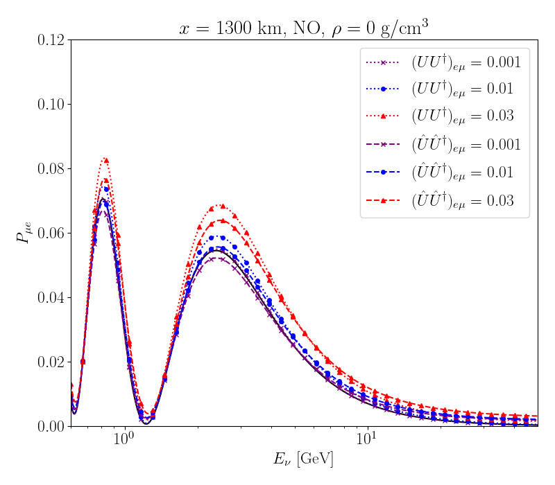
Figure 2: Comparison of the probability of $\nu_{\mu}\to\nu_{e}$ at $x=1300$ km in the vacuum as a function of neutrino energy $E_{\nu}$ between the high scale nonunitarity scenario (dotted lines) and low scale nonunitarity scenario (dashed lines) with $(UU^{\dagger})_{ee}=(UU^{\dagger})_{\mu\mu}=(\hat{U}\hat{U}^{\dagger})_{ee}=(\hat{U}\hat{U}^{\dagger})_{\mu\mu}=0.96$. The solid black line is the standard three-flavor unitarity scenario.

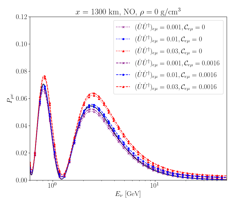
Figure 3: The probability of $\nu_{\mu}\to\nu_{e}$ at $x=1300$ km in the vacuum as a function of neutrino energy $E_{\nu}$ for low scale nonunitarity scenario with $(\hat{U}\hat{U}^{\dagger})_{ee}=(\hat{U}\hat{U}^{\dagger})_{\mu\mu}=0.96$ by setting the leaking term to be the maximum ${\cal C}_{e\mu}=0.0016$ (dashed lines) and the minimum ${\cal C}_{e\mu}=0$ (dotted lines). The solid black line is the standard three-flavor unitarity scenario.

In the neutrino experiments, the number of observed of neutrinos at the detector can be written as

$$N_{\beta\alpha} = \sigma_{\beta}P_{\beta\alpha}\left(x\right)\phi_{\alpha},$$ (84)

where $\phi_{\alpha}$ is the $\nu_{\alpha}$ neutrino flux at production and $\sigma_{\beta}$ is the detection cross section of $\nu_{\beta}$ and the energy dependence of all the terms are left implicit. In order to determine $P_{\beta\alpha}\left(x\right)$ from $N_{\beta\alpha}$, it is crucial to have precise determination of $\sigma_{\beta}\times\phi_{\alpha}$. To mitigate the uncertainty in flux determination, one can take the ratio of measurement in a far detector placed at $x_{1}$ and a near detector placed at $x_{0}$

$$\frac{N_{\beta\alpha}\left(x_{1}\right)}{N_{\alpha\alpha}\left(x_{0}\right)} = \frac{\sigma_{\beta}P_{\beta\alpha}\left(x_{1}\right)\phi_{\alpha}}{\sigma_{\alpha}P_{\alpha\alpha}\left(x_{0}\right)\phi_{\alpha}}=\frac{\sigma_{\beta}P_{\beta\alpha}\left(x_{1}\right)}{\sigma_{\alpha}P_{\alpha\alpha}\left(x_{0}\right)}.$$ (85)

For the high and low scale nonunitarity scenarios with $x_{0}\ll E/m_{i}^{2}$ for all $i$, eqs. (77) and (78) are

$$P_{\alpha\alpha}^{\textrm{high}}\left(x_{0}\right) \simeq (\overline{U}\,\overline{U}^{\dagger}\hat{P}_{\alpha}\overline{U}\,\overline{U}^{\dagger})_{\alpha\alpha}+\mathcal{O}\left(x_{0}^{2}m_{i}^{4}/E^{2}\right),$$ (86)

$$P_{\alpha\alpha}^{\textrm{low}}\left(x_{0}\right) \simeq 1-\mathcal{O}\left(x_{0}^{2}m_{i}^{4}/E^{2}\right),$$ (87)

which give

$$\left.\frac{N_{\beta\alpha}\left(x_{1}\right)}{N_{\alpha\alpha}\left(x_{0}\right)}\right|_{\textrm{high}} \simeq \frac{\sigma_{\beta}}{\sigma_{\alpha}}\frac{P_{\beta\alpha}^{\textrm{high}}\left(x_{1}\right)}{(\overline{U}\,\overline{U}^{\dagger}\hat{P}_{\alpha}\overline{U}\,\overline{U}^{\dagger})_{\alpha\alpha}},$$ (88)

$$\left.\frac{N_{\beta\alpha}\left(x_{1}\right)}{N_{\alpha\alpha}\left(x_{0}\right)}\right|_{\textrm{low}} \simeq \frac{\sigma_{\beta}}{\sigma_{\alpha}}P_{\beta\alpha}^{\textrm{low}}\left(x_{1}\right).$$ (89)

With dedicated measurements of $\sigma_{\beta}$ and $\sigma_{\alpha}$, the two scenarios can be distinguished from each other. In the low scale nonunitarity scenario with $x_{0}\gg E/m_{i}^{2}$ for $i>3$ such that the fast oscillations can be averaged out, eq. (80) gives

$$P_{\alpha\alpha}^{\textrm{low,ave}}\left(x_{0}\right) \simeq {\cal C}_{\alpha\alpha}+\left|\sum_{i=1}^{3}\hat{U}_{\alpha i}\hat{U}_{\alpha i}^{*}\right|^{2}-\mathcal{O}\left(x_{0}^{2}m_{i}^{4}/E^{2}\right).$$ (90)

In this case, one has

$$\left.\frac{N_{\beta\alpha}\left(x_{1}\right)}{N_{\alpha\alpha}\left(x_{0}\right)}\right|_{\textrm{low,ave}} \simeq \frac{\sigma_{\beta}}{\sigma_{\alpha}}\frac{P_{\beta\alpha}^{\textrm{low,ave}}\left(x_{1}\right)}{{\cal C}_{\alpha\alpha}+\left|\sum_{i=1}^{3}\hat{U}_{\alpha i}\hat{U}_{\alpha i}^{*}\right|^{2}}.$$ (91)

which can be differentiated from eqs. (88) and  (89). This type of arrangement has been planned in the upcoming neutrino experiments DUNE DUN and T2HK T2H .

Besides through neutrino oscillation experiments, the synergy with constraints from the electroweak precision measurements is needed to discover high scale nonunitarity Antusch and Fischer (2014); Fernandez-Martinez et al. (2016) or low scale nonunitarity de Gouvêa and Kobach (2016). If $\left(UU^{\dagger}\right)_{ee}=\left(UU^{\dagger}\right)_{\mu\mu}=\left(UU^{\dagger}\right)_{\tau\tau}\neq 1$, one can measure this deviation by comparing the leptonic weak processes with the hadronic weak processes. For instance, while absolute lifetimes of $\mu^{\pm}$, $\pi^{\pm}$, $K^{\pm}$ and $K^{0}$ will be affected, the leptonic branching ratios will be the same. For $K^{\pm}$ and $K^{0}$, the branching ratios to hadronic and leptonic channels will be modified. If $\left(UU^{\dagger}\right)_{ee}\neq\left(UU^{\dagger}\right)_{\mu\mu}\neq\left(UU^{\dagger}\right)_{\tau\tau}\neq 1$, lepton universality is broken and one can measure this by studying different leptonic weak processes. The reader can refer to refs. Antusch and Fischer (2014); Fernandez-Martinez et al. (2016); de Gouvêa and Kobach (2016) for more details.

V.2 In matter

Now let us consider the scenario with matter effect. For high scale nonunitarity scenario, eq. (32) is just

$$\widetilde{H}^{\textrm{high}} = \Delta+\overline{U}^{-1}V\overline{U}^{\dagger,-1},$$ (92)

where $\overline{U}$ spans over 3 flavors. According to theorem proved earlier, in the hidden nonunitarity scenario $\left(UU^{\dagger}\right)_{\alpha\beta}=0$ for all $\alpha\neq\beta$, $\overline{U}$ is unitary and hence $\widetilde{H}^{\textrm{high}}$ is indistinguishable from the unitarity scenario. Moreover, this result holds for an arbitrary potential $V\left(x\right)$ since one can always split $x$ into intervals small enough that $V\left(x\right)$ is constant and then construct the full solution as in eq. (46). So even in matter, for the high scale nonunitarity scenario, nonunitarity effect is proportional to $\left(UU^{\dagger}\right)_{\alpha\beta}$ for $\alpha\neq\beta$ as encapsulated in eq. (59).

In low scale nonunitarity scenario, $\overline{\mathbf{U}}^{-1}=\mathbf{U}^{\dagger}$, eq. (32) becomes

$$\widetilde{H}^{\textrm{low}} = \Delta+\mathbf{U}^{\dagger}V\mathbf{U}.$$ (93)

First of all, since $\mathbf{U}$ is unitary, eqs. (53) and (54) remain matter invariant as long as $V$ is diagonal and hence the resulting matter invariant identities hold. Next, besides the two possibilities discussed in the vacuum case, now we have a new handle: with the matter effect, the difference appear at leading order in small unitarity violating parameter $\epsilon$ in which the leading Hamiltonian $\widetilde{H}^{\textrm{low}}$ is given by Fong et al. (2019)

$$\widetilde{H}^{\textrm{low},0} = \Delta+\hat{U}^{\dagger}V\hat{U}.$$ (94)

Comparing the $\widetilde{H}^{\textrm{high}}$ and $\widetilde{H}^{\textrm{low},0}$, the difference is proportional to

$$\widetilde{H}^{\textrm{low},0}-\widetilde{H}^{\textrm{high}} = \hat{U}^{\dagger}V\hat{U}-U^{-1}\kappa V\kappa U^{\dagger,-1},$$ (95)

where we have written $\overline{U}=\kappa^{-1}U$ with $\kappa\equiv\textrm{diag}\left(\sqrt{\left(UU^{\dagger}\right)_{ee}},\sqrt{\left(UU^{\dagger}\right)_{\mu\mu}},\sqrt{\left(UU^{\dagger}\right)_{\tau\tau}}\right)$. Notice that the mapping of $\kappa^{-1}U$ to $\hat{U}$ in the vacuum case does not work in the presence of matter i.e. eq. (95) does not become zero.

Let us suppose that $\hat{U}=U$, i.e., the nonunitarity effect results in an identical $3\times 3$ submatrix. Then $\widetilde{H}^{\textrm{low},0}-\widetilde{H}^{\textrm{high}}\neq 0$ and matter effects will result in different eigenvalues and eigenvectors. For $0\leq x<x_{1}$ where $V$ is constant, we can solve for the oscillation amplitude $S$ in the flavor basis (41) as follows

$$S_{\beta\alpha}^{\textrm{high}} = \kappa_{\beta}^{-1}\kappa_{\alpha}^{-1}\sum_{i,j,k}U_{\beta i}U_{\alpha j}^{*}X_{ik}^{\textrm{high}}X_{jk}^{\textrm{high},*}e^{-i\lambda_{k}^{\textrm{high}}x},$$ (96)

$$S_{\beta\alpha}^{\textrm{low},0} = \sum_{i,j,k}U_{\beta i}U_{\alpha j}^{*}X_{ik}^{\textrm{low}}X_{jk}^{\textrm{low},*}e^{-i\lambda_{k}^{\textrm{low}}x}.$$ (97)

Hence, besides the amplitudes, the frequencies are different due to different eigenvalues $\lambda_{k}$.

To minimize the difference in matter potential, let us make a different choice $\hat{U}=\kappa U^{\dagger,-1}$ such that $\widetilde{H}^{\textrm{low},0}=\widetilde{H}^{\textrm{high}}$. In this case, $\widetilde{H}^{\textrm{high}}$ and $\widetilde{H}^{\textrm{low},0}$ will have exactly the same eigenvalues $\lambda_{k}$ and are diagonalized by the same unitary matrix $X$. So, we have

$$S_{\beta\alpha}^{\textrm{high}} = \kappa_{\beta}^{-1}\kappa_{\alpha}^{-1}\sum_{i,j,k}U_{\beta i}U_{\alpha j}^{*}X_{ik}X_{jk}^{*}e^{-i\lambda_{k}x},$$ (98)

$$S_{\beta\alpha}^{\textrm{low},0} = \kappa_{\beta}\kappa_{\alpha}\sum_{i,j,k}\left(U^{\dagger,-1}\right)_{\beta i}\left(U^{\dagger,-1}\right)_{\alpha j}^{*}X_{ik}X_{jk}^{*}e^{-i\lambda_{k}x},$$ (99)

where the differences are only in the amplitudes. Further difference between high scale and low scale nonunitarity scenarios comes from $(\hat{P}_{\beta})_{\xi\lambda}$ in eq. (42) just like in the vacuum case.

In Figure 4, we show identical situation with Figure 2 except with a constant matter density of $3$ g/cm³. Overall, the matter effect enhances the differences between the high scale and low scale nonunitarity scenarios as expected. We also observe that with decreasing modulus of $\left(UU^{\dagger}\right)_{e\mu}$, the high scale nonunitarity scenario approaches the unitarity scenario (the black line) while this does not happen for the low scale nonunitarity scenario. In Figure 5, we consider earth core-crossing neutrinos in a simplified PREM model (see appendix A of Fong (2022)) with high scale nonunitarity parameters $\left(UU^{\dagger}\right)_{ee}=\left(UU^{\dagger}\right)_{\mu\mu}=0.96$, $\left(UU^{\dagger}\right)_{\tau\tau}=1$, $\left(UU^{\dagger}\right)_{e\tau}=\left(UU^{\dagger}\right)_{\mu\tau}=0$ and $\left(UU^{\dagger}\right)_{e\mu}=\left\{10^{-3},10^{-2},0.03\right\}$. For low scale nonunitarity parameters, on the left plot, we set $\hat{U}=U$ while on the right plot, we set $\hat{U}=\kappa U^{\dagger,-1}$. These represent the two extreme cases where for $\hat{U}=U$, the difference in matter between the two scenarios is maximal while for $\hat{U}=\kappa U^{\dagger,-1}$, the matter effect is identical.

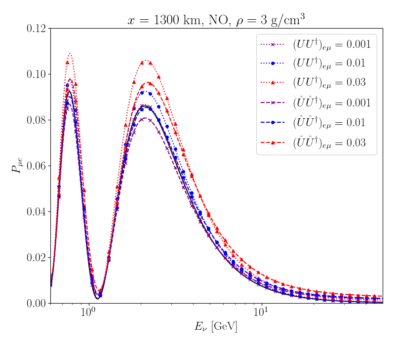
Figure 4: Same as Figure 2 but in a constant matter density of 3 g/cm³.

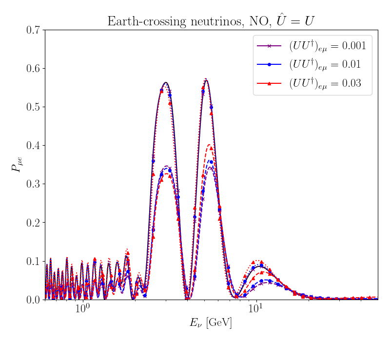
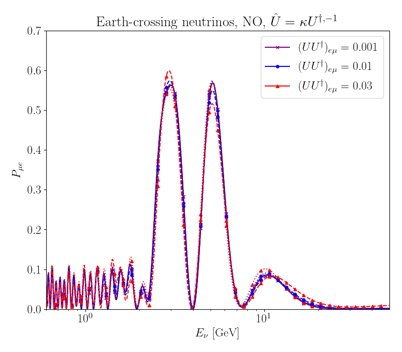
Figure 5: Comparison of the probability of $\nu_{\mu}\to\nu_{e}$ as a function of neutrino energy $E_{\nu}$ using the simplified PREM model for neutrino crossing through the Earth core between high scale nonunitarity scenario (dotted lines) and low scale nonunitarity scenario (dashed lines). We have shown the two extreme choices $\hat{U}=U$ (left plot) and $\hat{U}=\kappa U^{\dagger,-1}$ (right plot). See text for further explanation. The solid black line is the standard three-flavor unitarity scenario.

VI Conclusions

In this work, we have derived analytical oscillation probability amplitude for arbitrary flavors of neutrinos without assuming a unitary $\mathbf{U}$. With this result, we have proven a theorem that as long as $\left(\mathbf{U}\mathbf{U}^{\dagger}\right)_{\beta\alpha}=0$ for all $\alpha\neq\beta$, the scenario is indistinguishable from a unitarity scenario in an arbitrary matter potential. We further derive a general identity (59) which reduces to (60) in the vacuum and vanishes in the unitarity scenario.

We have highlighted the differences between high scale and low scale nonunitarity scenarios in neutrino oscillations, which are to be expected since in the former case, all new physics are integrated out while in the latter, new states are accessible though not necessarily remain coherent to result in oscillations. The first difference is that there is a zero distance effect for high scale nonunitarity scenario due to nonorthogonal flavor states, while it is absence for low scale nonunitarity scenario. On the one hand, although high scale nonunitarity scenario is model-independent (all the effects are fully captured by a nonunitary $U$), nonunitarity effects are proportional to $\left(UU^{\dagger}\right)_{\beta\alpha}$ for $\alpha\neq\beta$ and will be suppressed accordingly if the off-diagonal elements are small. On the other hand, while low scale nonunitarity scenario is model-dependent (depending on the properties of the new states), an almost model-independent scenario can be obtained if oscillations involving the new states can be averaged out and nonunitarity effects can be captured by a nonunitary $\hat{U}$ and a leaking term ${\cal C}_{\alpha\beta}$. In this case, low scale nonunitarity effects remain even in the limit of vanishing $(\hat{U}\hat{U}^{\dagger})_{\beta\alpha}$ for all $\alpha\neq\beta$.

The next important result for high scale nonunitarity is that despite $U$ being nonunitary due to new physics, we have shown that the theory remains unitary since the Hamiltonian in the vacuum mass basis is Hermitian and is related to the non-Hermitian Hamiltonian in the flavor basis through similarity transformation with the nonunitary $U$. In order words, unitarity violation is only apparent but we will continue to call this scenario high scale unitarity violation in reference to nonunitary $U$. We have constructed explicitly neutrino oscillation probability which always respect unitarity even though $U$ is not unitary.

In summary, high scale and low scale nonunitarity scenarios are distinct, testing them carefully in the neutrino oscillation experiments will certainly give clues to what lies beyond the SM.

VII Acknowledgments

C.S.F. acknowledges the support by grant 2019/11197-6 and 2022/00404-3 from São Paulo Research Foundation (FAPESP), and grant 301271/2019-4 and 407149/2021-0 from National Council for Scientific and Technological Development (CNPq). He would like to thank Hisakazu Minakata and Celso Nishi for reading and commenting on the manuscript. He also acknowledges support from the ICTP through the Associates Programme (2023-2028) while the revised version of this work was being completed.

Appendix A Nonorthogonal basis

Let us expand in an arbitrary state $\left|\psi\right\rangle$ in a nonorthogonal but normalized basis $\{\left|\alpha\right\rangle\}$

$$\left|\psi\right\rangle = \sum_{\alpha}c_{\alpha}\left|\alpha\right\rangle.$$ (100)

Multiplying the above by $\left\langle\beta\right|$ and define ${\cal N}_{\beta\alpha}\equiv\left\langle\beta|\alpha\right\rangle$, we can solve for $c_{\alpha}$ as follows

$$c_{\alpha} = \sum_{\beta}({\cal N}^{-1})_{\alpha\beta}\left\langle\beta|\psi\right\rangle.$$ (101)

Substituting the solution above back to into eq. (100), we obtain the completeness relation

$$\sum_{\alpha,\beta}\left|\alpha\right\rangle({\cal N}^{-1})_{\alpha\beta}\left\langle\beta\right| = \mathbf{I}.$$ (102)

Formally, we can take $g^{\alpha\beta}\equiv({\cal N}^{-1})_{\alpha\beta}$ as the metric which raises the indices of $\left|{}_{\alpha}\right\rangle\equiv\left|\alpha\right\rangle$ as $\left|{}^{\alpha}\right\rangle=g^{\alpha\beta}\left|{}_{\beta}\right\rangle$ to form the dual vector but we will not use this notation in this work. Applying the result above to case of neutrino flavor eigenstates which are not orthogonal in general, we identify ${\cal N}=\overline{\mathbf{U}}\,\overline{\mathbf{U}}^{\dagger}$.

Appendix B Projected probability operator

In refs. Leon and Neshyba (1988); Manning and De Leon (1990), the theory of projected probabilities on nonorthogonal states are developed. The basic idea is to first project $\left|\psi\right\rangle$ to a chosen $\left|\alpha\right\rangle$ and to the corresponding orthogonal component $\left|\alpha\right\rangle_{\perp}$. Then the orthogonal component is further projected to the (hyper)plane formed by the rest of the basis states and to the orthogonal component to this (hyper)plane. And this new orthogonal component is again projected to $\left|\alpha\right\rangle$ and $\left|\alpha\right\rangle_{\perp}$ and so on. The procedure can be written down as follows

$$\left|\psi\right\rangle = \frac{1}{2}\left(p_{\alpha}\left|\psi\right\rangle+q_{\alpha}\left|\psi\right\rangle\right)+\frac{1}{2}\left(p_{\not\alpha}\left|\psi\right\rangle+q_{\not\alpha}\left|\psi\right\rangle\right)$$ (103)

$$= \frac{1}{2}\left(p_{\alpha}\left|\psi\right\rangle+p_{\not\alpha}q_{\alpha}\left|\psi\right\rangle+q_{\not\alpha}q_{\alpha}\left|\psi\right\rangle\right)+\frac{1}{2}\left(p_{\not\alpha}\left|\psi\right\rangle+p_{\alpha}q_{\not\alpha}\left|\psi\right\rangle+q_{\alpha}q_{\not\alpha}\left|\psi\right\rangle\right)$$

$$= \frac{1}{2}\left(p_{\alpha}\left|\psi\right\rangle+p_{\not\alpha}q_{\alpha}\left|\psi\right\rangle+p_{\alpha}q_{\not\alpha}q_{\alpha}\left|\psi\right\rangle+...\right)+\frac{1}{2}\left(p_{\not\alpha}\left|\psi\right\rangle+p_{\alpha}q_{\not\alpha}\left|\psi\right\rangle+p_{\not\alpha}q_{\alpha}q_{\not\alpha}\left|\psi\right\rangle+...\right)$$

$$= \frac{1}{2}\left[p_{\alpha}\left(\mathbf{I}+q_{\not\alpha}+q_{\not\alpha}q_{\alpha}+...\right)\right]\left|\psi\right\rangle+\frac{1}{2}\left[p_{\not\alpha}\left(\mathbf{I}+q_{\alpha}+q_{\alpha}q_{\not\alpha}+...\right)\right]\left|\psi\right\rangle,$$

where

$$p_{\alpha} \equiv \left|\alpha\right\rangle\left\langle\alpha\right|,\;\;q_{\alpha}\equiv\mathbf{I}-p_{\alpha},$$ (104)

and $p_{\not\alpha}$ is the projection on to the hyperplane spanned by the rest of bases besides $\left|\alpha\right\rangle$ and $q_{\not\alpha}\equiv\mathbf{I}-p_{\not\alpha}$. From the above, we have

$$P_{\alpha}\left|\psi\right\rangle = c_{\alpha}\left|\alpha\right\rangle=\frac{1}{2}\left[p_{\alpha}\left(\mathbf{I}+q_{\not\alpha}+q_{\not\alpha}q_{\alpha}+...\right)\right]\left|\psi\right\rangle.$$ (105)

By construction, the sum of absolute square of each operator is unity

$$\frac{1}{2}\left(p_{\alpha}+q_{\not\alpha}p_{\alpha}q_{\not\alpha}+q_{\alpha}q_{\not\alpha}p_{\alpha}q_{\not\alpha}q_{\alpha}+...\right)+\frac{1}{2}\left(p_{\not\alpha}+q_{\alpha}p_{\not\alpha}q_{\alpha}+q_{\not\alpha}q_{\alpha}p_{\not\alpha}q_{\alpha}q_{\not\alpha}+...\right) = \mathbf{I}.$$ (106)

Hence, we can define the probability operator of measuring $\left|\alpha\right\rangle$ in $\left|\psi\right\rangle$ expanded in the basis $\left|\alpha\right\rangle$

$$\hat{P}_{\alpha\alpha} \equiv \frac{1}{2}\left(p_{\alpha}+q_{\not\alpha}p_{\alpha}q_{\not\alpha}+q_{\alpha}q_{\not\alpha}p_{\alpha}q_{\not\alpha}q_{\alpha}+...\right).$$ (107)

The second operator can be further decomposed as projection onto $\left|\beta\right\rangle$ and $\left|{\not\beta}\right\rangle$ where $\beta,{\not\beta}\subset{\not\alpha}$ to construct $\hat{P}_{\beta\alpha}$. For $n\leq 3$, we can write down the closed form of probability operators.

B.1 Two-state system

For $n=2$, $\alpha,{\not\alpha}=\left\{1,2\right\}$, we have only two operators $\hat{P}_{11}$ and $\hat{P}_{\not 22}$ corresponding to the two terms in eq. (106). Utilizing the identities $q_{2}q_{1}q_{2}\left|1\right\rangle=\left|{\cal N}_{12}\right|^{2}q_{2}\left|1\right\rangle$ and $q_{1}q_{2}q_{1}\left|2\right\rangle=\left|{\cal N}_{12}\right|^{2}q_{1}\left|2\right\rangle$, we have a converging geometric series with $\left|N_{12}\right|^{2}<1$ and eq. (107) becomes

$$\left(p_{\alpha}\right)_{\left\{1,2\right\}} \equiv \hat{P}_{\alpha\alpha}=\frac{1}{2}\left(p_{\alpha}+\frac{q_{\not\alpha}p_{\alpha}q_{\not\alpha}+q_{\alpha}q_{\not\alpha}p_{\alpha}q_{\not\alpha}q_{\alpha}}{1-\left|{\cal N}_{12}\right|^{4}}\right),$$ (108)

where the subscript $\left\{1,2\right\}$ denotes the basis states. So $\left(p_{\alpha}\right)_{\left\{1,2\right\}}$ is the probability operator which gives the probability of a state $\left|\psi\right\rangle$ being found along $\left|\alpha\right\rangle$ given by $\left\langle\psi\right|\left(p_{\alpha}\right)_{\left\{1,2\right\}}\left|\psi\right\rangle$. After some algebra, we arrive at

$$\left(p_{\alpha}\right)_{\left\{1,2\right\}} = \frac{1}{1-\left|{\cal N}_{12}\right|^{4}}\left[p_{\alpha}+\left|{\cal N}_{12}\right|^{2}p_{\not\alpha}-\frac{1+\left|{\cal N}_{12}\right|^{2}}{2}\left\{p_{\alpha},p_{\not\alpha}\right\}\right],$$ (109)

where $\left\{p_{\alpha},p_{\not\alpha}\right\}=p_{\alpha}p_{\not\alpha}+p_{\not\alpha}p_{\alpha}$. Summing over $\alpha$, one obtain

$$\sum_{\alpha=1}^{2}\left(p_{\alpha}\right)_{\left\{1,2\right\}} = \frac{p_{1}+p_{2}-\left\{p_{1},p_{2}\right\}}{1-\left|{\cal N}_{12}\right|^{2}}=\mathbf{I},$$ (110)

which follows from eq. (102).

The probability of $\left|\psi\right\rangle\to\left|\alpha\right\rangle$ is then given by

$$P_{\psi\to\alpha} = \left\langle\psi\right|\left(p_{\alpha}\right)_{\left\{1,2\right\}}\left|\psi\right\rangle$$ (111)

$$= \sum_{\xi,\zeta,\eta,\lambda}\left\langle\psi|\xi\right\rangle\left({\cal N}^{-1}\right)_{\xi\zeta}\left\langle\zeta\right|\left(p_{\alpha}\right)_{\left\{1,2\right\}}\left|\eta\right\rangle\left({\cal N}^{-1}\right)_{\eta\lambda}\left\langle\lambda|\psi\right\rangle$$

$$\equiv \left(S^{\dagger}D_{\alpha}S\right)_{\psi\psi},$$

where we have defined

$$S_{\lambda\psi} \equiv \left\langle\lambda|\psi\right\rangle,$$ (112)

$$\left[D_{\alpha}\right]_{\xi\lambda} \equiv \sum_{\zeta,\eta}\left({\cal N}^{-1}\right)_{\xi\zeta}\left\langle\zeta\right|\left(p_{\alpha}\right)_{12}\left|\eta\right\rangle\left({\cal N}^{-1}\right)_{\eta\lambda}.$$ (113)

In the second equality of the probability, we have used the completeness relation given by eq. (102). For the two-flavor system, we have

$${\cal N} = \left(\begin{array}[]{cc}1&{\cal N}_{12}\\ {\cal N}_{12}^{*}&1\end{array}\right),\quad{\cal N}^{-1}=\frac{1}{1-\left|{\cal N}_{12}\right|^{2}}\left(\begin{array}[]{cc}1&-{\cal N}_{12}\\ -{\cal N}_{12}^{*}&1\end{array}\right).$$ (118)

Evaluating directly the matrix elements of $D_{\alpha}$, we have

$$\left[D_{\alpha}\right]_{\xi\lambda} = \frac{1}{1-\left|{\cal N}_{12}\right|^{4}}\bigg{[}\delta_{\xi\alpha}\delta_{\alpha\lambda}+\left|{\cal N}_{12}\right|^{2}\delta_{\xi\not\alpha}\delta_{\not\alpha\lambda}$$ (119)

$$-\frac{1+\left|{\cal N}_{12}\right|^{2}}{2}\left(\delta_{\xi\alpha}{\cal N}_{\alpha\not\alpha}\delta_{\not\alpha\lambda}+\delta_{\xi\not\alpha}{\cal N}_{\not\alpha\alpha}\delta_{\alpha\lambda}\right)\bigg{]},$$

or

$$\left[D_{\alpha}\right]_{\xi\lambda} = \begin{cases}{\displaystyle 1+\frac{\left|{\cal N}_{12}\right|^{4}}{1-\left|{\cal N}_{12}\right|^{4}}},&\xi=\lambda=\alpha\\ {\displaystyle\frac{\left|{\cal N}_{12}\right|^{2}}{1-\left|{\cal N}_{12}\right|^{4}}},&\xi=\lambda\neq\alpha\\ {\displaystyle-\frac{1}{2}\frac{{\cal N}_{\xi\lambda}}{1-\left|{\cal N}_{12}\right|^{2}}},&\xi\neq\lambda\;\textrm{and}\;\xi=\alpha\;\textrm{or}\;\lambda=\alpha\end{cases}.$$ (120)

In the absence of nonorthogonality, the standard result is recovered $\left(p_{\alpha}\right)_{\left\{1,2\right\}}=p_{\alpha}$, $\left[D_{\alpha}\right]_{\xi\lambda}=\delta_{\xi\alpha}\delta_{\alpha\lambda}$ and $P_{\psi\to\alpha}=\left|S_{\alpha\psi}\right|^{2}$.

B.2 Three-state system

For $n=3$, in order to obtain symmetrize probability operator, one repeats the procedure of eq. (103) projecting $\left|\psi\right\rangle$ into $\left|\beta\right\rangle\neq\left|\alpha\right\rangle$ and the corresponding plane not containing $\left|\beta\right\rangle$ and there are altogether 3 choices. Doing so, we obtain the symmetrize probability operator on $\left|\alpha\right\rangle$ as

$$\hat{P}_{\alpha} = \frac{1}{3}\sum_{\beta}\hat{P}_{\alpha\beta},$$ (121)

where

$$\hat{P}_{\alpha\alpha} = \frac{1}{2}\left[p_{\alpha}+\frac{q_{\beta\gamma}p_{\alpha}q_{\beta\gamma}}{1-X_{\alpha}^{2}}+\frac{q_{\alpha}q_{\beta\gamma}p_{\alpha}q_{\beta\gamma}q_{\alpha}}{1-X_{\alpha}^{2}}\right],\quad\beta\neq\gamma;\beta,\gamma\neq\alpha,$$ (122)

$$\hat{P}_{\alpha\beta} = \frac{1}{2}\Biggl{[}\left(p_{\alpha}\right)_{\left\{\alpha,\gamma\right\}}+q_{\beta}\left(p_{\alpha}\right)_{\left\{\alpha,\gamma\right\}}q_{\beta}$$ (124)

$$\!\!\!\!\!+\frac{q_{\alpha\gamma}p_{\beta}\left(p_{\alpha}\right)_{\left\{\alpha,\gamma\right\}}p_{\beta}q_{\alpha\gamma}}{1-X_{\beta}^{2}}+\frac{q_{\beta}q_{\alpha\gamma}p_{\beta}\left(p_{\alpha}\right)_{\left\{\alpha,\gamma\right\}}p_{\beta}q_{\alpha\gamma}q_{\beta}}{1-X_{\beta}^{2}}\Biggr{]},\quad\beta\neq\alpha;\gamma\neq\left\{\alpha,\beta\right\},$$

with

$$p_{\beta\gamma} \equiv \frac{p_{\beta}+p_{\gamma}-\left\{p_{\beta},p_{\gamma}\right\}}{1-\left|{\cal N}_{\beta\gamma}\right|^{2}},\;\;q_{\beta\gamma}\equiv\mathbf{I}-p_{\beta\gamma},\;\;\;\gamma\neq\beta,$$ (125)

$$\left(p_{\alpha}\right)_{\left\{\alpha,\gamma\right\}} \equiv \frac{1}{1-\left|{\cal N}_{\alpha\gamma}\right|^{4}}\left[p_{\alpha}+\left|{\cal N}_{\alpha\gamma}\right|^{2}p_{\not\alpha}-\frac{1+\left|{\cal N}_{\alpha\gamma}\right|^{2}}{2}\left\{p_{\alpha},p_{\not\alpha}\right\}\right],\quad\gamma\neq\alpha,$$ (126)

$$X_{\alpha} \equiv 1-\frac{\det{\cal N}}{\det{\cal N}_{\alpha}},$$ (127)

In the last relation above, ${\cal N}_{\alpha}$ is the $2\times 2$ matrix constructed excluding the basis $\left|\alpha\right\rangle$. The operator $p_{\beta\gamma}$ projects a state onto the $\left\{\beta,\gamma\right\}$-plane spanned by two orthonormal vectors $\left|\beta\right\rangle$ and $\left(1-{\cal N}_{\beta\gamma}^{2}\right)^{-1/2}q_{\beta}\left|\gamma\right\rangle$. The second operator $\left(p_{\alpha}\right)_{\left\{\alpha,\gamma\right\}}$ has the same form as the probability operator (109) that we have found in the two-flavor case. For the three-flavor case, we can write

$${\cal N} = \left(\begin{array}[]{ccc}1&{\cal N}_{12}&{\cal N}_{13}\\ {\cal N}_{12}^{*}&1&{\cal N}_{23}\\ {\cal N}_{13}^{*}&{\cal N}_{23}^{*}&1\end{array}\right),$$ (131)

$${\cal N}^{-1} = \frac{1}{\det{\cal N}}\left(\begin{array}[]{ccc}1-\left|{\cal N}_{23}\right|^{2}&-{\cal N}_{12}+{\cal N}_{13}{\cal N}_{23}^{*}&-{\cal N}_{13}+{\cal N}_{12}{\cal N}_{23}\\ -{\cal N}_{12}^{*}+{\cal N}_{13}^{*}{\cal N}_{23}&1-\left|{\cal N}_{13}\right|^{2}&-{\cal N}_{23}+{\cal N}_{13}{\cal N}_{12}^{*}\\ -{\cal N}_{13}^{*}+{\cal N}_{12}^{*}{\cal{\cal N}}_{23}^{*}&-{\cal N}_{23}^{*}+{\cal N}_{13}^{*}{\cal N}_{12}&1-\left|{\cal N}_{12}\right|^{2}\end{array}\right),$$ (135)

$$\det{\cal N} = -\left|{\cal N}_{23}\right|^{2}-\left|{\cal N}_{12}\right|^{2}-\left|{\cal N}_{13}\right|^{2}+{\cal N}_{12}{\cal N}_{13}^{*}{\cal N}_{23}+{\cal N}_{13}{\cal N}_{12}^{*}{\cal N}_{23}^{*},$$ (136)

$$\det{\cal N}_{1} = 1-\left|{\cal N}_{23}\right|^{2},\;\det{\cal N}_{2}=1-\left|{\cal N}_{13}\right|^{2},\;\det{\cal N}_{3}=1-\left|{\cal N}_{12}\right|^{2}.$$ (137)

One can check explicitly that

$$\sum_{\alpha=1}^{3}\hat{P}_{\alpha} = \frac{1}{3}\sum_{\alpha,\beta}\hat{P}_{\alpha\beta}=\frac{1}{\det{\cal N}}\sum_{\alpha}\left[p_{\alpha}\det{\cal N}_{\alpha}+\sum_{\beta\neq\alpha}\left(-p_{\alpha}p_{\beta}+p_{\alpha}p_{\gamma}p_{\beta}\right)\right]=\mathbf{I},$$ (138)

which follows from eq. (102).

The probability of $\left|\psi\right\rangle\to\left|\alpha\right\rangle$ now becomes

$$P_{\psi\to\alpha} = \langle\psi|\hat{P}_{\alpha}|\psi\rangle\equiv\frac{1}{3}\left[S^{\dagger}\left(E_{\alpha}+\sum_{\beta\neq\alpha}F_{\alpha\beta}\right)S\right]_{\psi\psi},$$ (139)

where we have defined

$$\left[E_{\alpha}\right]_{\xi\lambda} \equiv \sum_{\zeta,\eta}\left({\cal N}^{-1}\right)_{\xi\zeta}\left\langle\zeta\right|\hat{P}_{\alpha\alpha}\left|\eta\right\rangle\left({\cal N}^{-1}\right)_{\eta\lambda},$$ (140)

$$\left[F_{\alpha\beta}\right]_{\xi\lambda} \equiv \sum_{\zeta,\eta}\left({\cal N}^{-1}\right)_{\xi\zeta}\left\langle\zeta\right|\hat{P}_{\alpha\beta}\left|\eta\right\rangle\left({\cal N}^{-1}\right)_{\eta\lambda}.$$ (141)

Evaluating explicitly the matrix elements, we obtain

$$\left[E_{\alpha}\right]_{\xi\lambda} = \begin{cases}{\displaystyle 1+\frac{X_{\alpha}^{2}}{1-X_{\alpha}^{2}}},&\xi=\lambda=\alpha\\ {\displaystyle\frac{\left|{\cal N}_{\alpha\xi}-{\cal N}_{\alpha\gamma}{\cal N}_{\gamma\xi}\right|^{2}}{\left(\det{\cal N}_{\alpha}\right)^{2}\left(1-X_{\alpha}^{2}\right)},\;\gamma\neq\left\{\alpha,\xi\right\}},&\xi=\lambda\neq\alpha\\ {\displaystyle-\frac{1}{2}\frac{{\cal N}_{\xi\lambda}-{\cal N}_{\xi\gamma}{\cal N}_{\gamma\lambda}}{\det{\cal N}}},\;\gamma\neq\left\{\alpha,\xi\right\},&\xi\neq\lambda\;\textrm{and}\;\xi=\alpha\;\textrm{or}\;\lambda=\alpha\\ {\displaystyle\frac{\left({\cal N}_{\alpha\lambda}-{\cal N}_{\alpha\xi}{\cal N}_{\xi\lambda}\right)\left({\cal N}_{\xi\alpha}-{\cal N}_{\xi\lambda}{\cal N}_{\lambda\alpha}\right)}{\left(\det{\cal N}_{\alpha}\right)^{2}\left(1-X_{\alpha}^{2}\right)}},&\xi\neq\lambda\;\textrm{and}\;\left\{\xi,\lambda\right\}\neq\alpha\end{cases},$$ (142)

and for $\alpha\neq\beta$ and $\gamma\neq\left\{\alpha,\beta\right\}$

$$\left[F_{\alpha\beta}\right]_{\xi\lambda} = \begin{cases}{\displaystyle\frac{1}{1-\left|{\cal N}_{\alpha\gamma}\right|^{4}}+\frac{\left\langle\beta\right|\left(p_{\alpha}\right)_{\alpha\gamma}\left|\beta\right\rangle\left|{\cal N}_{\alpha\beta}-{\cal N}_{\alpha\gamma}{\cal N}_{\gamma\beta}\right|^{2}}{\left(\det{\cal N}_{\beta}\right)^{2}\left(1-X_{\beta}^{2}\right)}},&\xi=\lambda=\alpha\\ {\displaystyle\begin{split}-\frac{1}{2}\frac{1}{1-\left|{\cal N}_{\alpha\gamma}\right|^{4}}\left({\cal N}_{\xi\lambda}-\frac{1+\left|{\cal N}_{\alpha\gamma}\right|^{2}}{2}{\cal N}_{\xi\gamma}{\cal N}_{\gamma\lambda}\right)\\ -\frac{1}{2}\frac{\left\langle\beta\right|\left(p_{\alpha}\right)_{\left\{\alpha,\gamma\right\}}\left|\beta\right\rangle}{1-X_{\beta}^{2}}\frac{{\cal N}_{\xi\lambda}-{\cal N}_{\xi\gamma}{\cal N}_{\gamma\lambda}}{\det{\cal N}_{\beta}}\left(1+\left\langle\beta\right|p_{\alpha\gamma}\left|\beta\right\rangle\right)\end{split}},&\xi\lambda=\alpha\beta\;\textrm{or}\;\xi\lambda=\beta\alpha\\ {\displaystyle-\frac{1}{2}\frac{{\cal N}_{\xi\lambda}}{\det{\cal N}_{\beta}}+\frac{\left\langle\beta\right|\left(p_{\alpha}\right)_{\left\{\alpha,\gamma\right\}}\left|\beta\right\rangle\left({\cal N}_{\xi\beta}-{\cal N}_{\xi\lambda}{\cal N}_{\lambda\beta}\right)\left({\cal N}_{\beta\lambda}-{\cal N}_{\beta\xi}{\cal N}_{\xi\lambda}\right)}{\left(\det{\cal N}_{\beta}\right)^{2}\left(1-X_{\beta}^{2}\right)}},&\xi\lambda=\alpha\gamma\;\textrm{or}\;\xi\lambda=\gamma\alpha\\ {\displaystyle\frac{1}{2}\left[1+\frac{1+\left\langle\beta\right|p_{\alpha\gamma}\left|\beta\right\rangle^{2}}{1-X_{\beta}^{2}}\right]\left\langle\beta\right|\left(p_{\alpha}\right)_{\left\{\alpha,\gamma\right\}}\left|\beta\right\rangle},&\xi=\lambda=\beta\\ {\displaystyle\begin{split}-\frac{1}{2}\frac{1}{1-\left|{\cal N}_{\alpha\gamma}\right|^{4}}\left(\left|{\cal N}_{\alpha\gamma}\right|^{2}{\cal N}_{\xi\lambda}-\frac{1+\left|{\cal N}_{\alpha\gamma}\right|^{2}}{2}{\cal N}_{\xi\alpha}{\cal N}_{\alpha\lambda}\right)\\ -\frac{1}{2}\frac{\left\langle\beta\right|\left(p_{\alpha}\right)_{\left\{\alpha,\gamma\right\}}\left|\beta\right\rangle}{1-X_{\beta}^{2}}\frac{{\cal N}_{\xi\lambda}-{\cal N}_{\xi\alpha}{\cal N}_{\alpha\lambda}}{\det{\cal N}_{\beta}}\left(1+\left\langle\beta\right|p_{\alpha\gamma}\left|\beta\right\rangle\right)\end{split},}&\xi\lambda=\beta\gamma\;\textrm{or}\;\xi\lambda=\gamma\beta\\ {\displaystyle\frac{\left|{\cal N}_{\alpha\gamma}\right|^{2}}{1-\left|{\cal N}_{\alpha\gamma}\right|^{4}}+\frac{\left\langle\beta\right|\left(p_{\alpha}\right)_{\left\{\alpha,\gamma\right\}}\left|\beta\right\rangle\left|{\cal N}_{\gamma\beta}-{\cal N}_{\gamma\alpha}{\cal N}_{\alpha\beta}\right|^{2}}{\left(\det{\cal N}_{\beta}\right)^{2}\left(1-X_{\beta}^{2}\right)}},&\xi=\lambda=\gamma\end{cases},$$ (143)

where

$$\left\langle\beta\right|p_{\alpha\gamma}\left|\beta\right\rangle = \frac{\left|{\cal N}_{\alpha\beta}\right|^{2}+\left|{\cal N}_{\beta\gamma}\right|^{2}-2\textrm{Re}\left({\cal N}_{\beta\alpha}{\cal N}_{\alpha\gamma}{\cal N}_{\gamma\beta}\right)}{1-\left|{\cal N}_{\alpha\gamma}\right|^{2}},$$ (144)

$$\left\langle\beta\right|\left(p_{\alpha}\right)_{\left\{\alpha,\gamma\right\}}\left|\beta\right\rangle = \frac{\left|{\cal N}_{\alpha\beta}\right|^{2}+\left|{\cal N}_{\alpha\gamma}\right|^{2}\left|{\cal N}_{\beta\gamma}\right|^{2}-\left(1+\left|{\cal N}_{\alpha\gamma}\right|^{2}\right)\textrm{Re}\left({\cal N}_{\beta\alpha}{\cal N}_{\alpha\gamma}{\cal N}_{\gamma\beta}\right)}{1-\left|{\cal N}_{\alpha\gamma}\right|^{4}}.$$ (145)

References

- Esteban et al. (2020) Ivan Esteban, M. C. Gonzalez-Garcia, Michele Maltoni, Thomas Schwetz, and Albert Zhou, “The fate of hints: updated global analysis of three-flavor neutrino oscillations,” JHEP 09, 178 (2020), arXiv:2007.14792 [hep-ph] .
- (2) “NuFIT 5.2: Three-neutrino fit based on data available in November 2022,” .
- Weinberg (1979) Steven Weinberg, “Baryon and Lepton Nonconserving Processes,” Phys. Rev. Lett. 43, 1566–1570 (1979).
- Weinberg (1980) Steven Weinberg, “Varieties of Baryon and Lepton Nonconservation,” Phys. Rev. D 22, 1694 (1980).
- Antusch et al. (2006) S. Antusch, C. Biggio, E. Fernandez-Martinez, M. B. Gavela, and J. Lopez-Pavon, “Unitarity of the Leptonic Mixing Matrix,” JHEP 10, 084 (2006), arXiv:hep-ph/0607020 .
- Fernandez-Martinez et al. (2007) E. Fernandez-Martinez, M. B. Gavela, J. Lopez-Pavon, and O. Yasuda, “CP-violation from non-unitary leptonic mixing,” Phys. Lett. B 649, 427–435 (2007), arXiv:hep-ph/0703098 .
- Xing (2008) Zhi-zhong Xing, “Correlation between the Charged Current Interactions of Light and Heavy Majorana Neutrinos,” Phys. Lett. B 660, 515–521 (2008), arXiv:0709.2220 [hep-ph] .
- Goswami and Ota (2008) Srubabati Goswami and Toshihiko Ota, “Testing non-unitarity of neutrino mixing matrices at neutrino factories,” Phys. Rev. D 78, 033012 (2008), arXiv:0802.1434 [hep-ph] .
- Antusch et al. (2009) Stefan Antusch, Mattias Blennow, Enrique Fernandez-Martinez, and Jacobo Lopez-Pavon, “Probing non-unitary mixing and CP-violation at a Neutrino Factory,” Phys. Rev. D 80, 033002 (2009), arXiv:0903.3986 [hep-ph] .
- Xing (2012) Zhi-zhong Xing, “A full parametrization of the 6 X 6 flavor mixing matrix in the presence of three light or heavy sterile neutrinos,” Phys. Rev. D 85, 013008 (2012), arXiv:1110.0083 [hep-ph] .
- Escrihuela et al. (2015) F. J. Escrihuela, D. V. Forero, O. G. Miranda, M. Tortola, and J. W. F. Valle, “On the description of nonunitary neutrino mixing,” Phys. Rev. D 92, 053009 (2015), [Erratum: Phys.Rev.D 93, 119905 (2016)], arXiv:1503.08879 [hep-ph] .
- Parke and Ross-Lonergan (2016) Stephen Parke and Mark Ross-Lonergan, “Unitarity and the three flavor neutrino mixing matrix,” Phys. Rev. D 93, 113009 (2016), arXiv:1508.05095 [hep-ph] .
- Dutta and Ghoshal (2016) Debajyoti Dutta and Pomita Ghoshal, “Probing CP violation with T2K, NOA and DUNE in the presence of non-unitarity,” JHEP 09, 110 (2016), arXiv:1607.02500 [hep-ph] .
- Dutta et al. (2017) Debajyoti Dutta, Pomita Ghoshal, and Samiran Roy, “Effect of Non Unitarity on Neutrino Mass Hierarchy determination at DUNE, NOA and T2K,” Nucl. Phys. B 920, 385–401 (2017), arXiv:1609.07094 [hep-ph] .
- Fong et al. (2017) Chee Sheng Fong, Hisakazu Minakata, and Hiroshi Nunokawa, “A framework for testing leptonic unitarity by neutrino oscillation experiments,” JHEP 02, 114 (2017), arXiv:1609.08623 [hep-ph] .
- Ge et al. (2017) Shao-Feng Ge, Pedro Pasquini, M. Tortola, and J. W. F. Valle, “Measuring the leptonic CP phase in neutrino oscillations with nonunitary mixing,” Phys. Rev. D 95, 033005 (2017), arXiv:1605.01670 [hep-ph] .
- Blennow et al. (2017) Mattias Blennow, Pilar Coloma, Enrique Fernandez-Martinez, Josu Hernandez-Garcia, and Jacobo Lopez-Pavon, “Non-Unitarity, sterile neutrinos, and Non-Standard neutrino Interactions,” JHEP 04, 153 (2017), arXiv:1609.08637 [hep-ph] .
- Fong et al. (2019) Chee Sheng Fong, Hisakazu Minakata, and Hiroshi Nunokawa, “Non-unitary evolution of neutrinos in matter and the leptonic unitarity test,” JHEP 02, 015 (2019), arXiv:1712.02798 [hep-ph] .
- Martinez-Soler and Minakata (2020a) Ivan Martinez-Soler and Hisakazu Minakata, “Standard versus Non-Standard CP Phases in Neutrino Oscillation in Matter with Non-Unitarity,” PTEP 2020, 063B01 (2020a), arXiv:1806.10152 [hep-ph] .
- Martinez-Soler and Minakata (2020b) Ivan Martinez-Soler and Hisakazu Minakata, “Physics of parameter correlations around the solar-scale enhancement in neutrino theory with unitarity violation,” PTEP 2020, 113B01 (2020b), arXiv:1908.04855 [hep-ph] .
- Dutta and Roy (2021) Debajyoti Dutta and Samiran Roy, “Non-Unitarity at DUNE and T2HK with Charged and Neutral Current Measurements,” J. Phys. G 48, 045004 (2021), arXiv:1901.11298 [hep-ph] .
- Ellis et al. (2020) Sebastian A. R. Ellis, Kevin J. Kelly, and Shirley Weishi Li, “Current and Future Neutrino Oscillation Constraints on Leptonic Unitarity,” JHEP 12, 068 (2020), arXiv:2008.01088 [hep-ph] .
- Wang and Zhou (2022) Yilin Wang and Shun Zhou, “Non-unitary leptonic flavor mixing and CP violation in neutrino-antineutrino oscillations,” Phys. Lett. B 824, 136797 (2022), arXiv:2109.13622 [hep-ph] .
- Forero et al. (2021) D. V. Forero, C. Giunti, C. A. Ternes, and M. Tortola, “Nonunitary neutrino mixing in short and long-baseline experiments,” Phys. Rev. D 104, 075030 (2021), arXiv:2103.01998 [hep-ph] .
- Denton and Gehrlein (2022) Peter B. Denton and Julia Gehrlein, “New oscillation and scattering constraints on the tau row matrix elements without assuming unitarity,” JHEP 06, 135 (2022), arXiv:2109.14575 [hep-ph] .
- Agarwalla et al. (2022) Sanjib Kumar Agarwalla, Sudipta Das, Alessio Giarnetti, and Davide Meloni, “Model-independent constraints on non-unitary neutrino mixing from high-precision long-baseline experiments,” JHEP 07, 121 (2022), arXiv:2111.00329 [hep-ph] .
- Majumdar et al. (2022) Anirban Majumdar, Dimitrios K. Papoulias, Rahul Srivastava, and José W. F. Valle, “Physics implications of recent Dresden-II reactor data,” Phys. Rev. D 106, 093010 (2022), arXiv:2208.13262 [hep-ph] .
- Acero et al. (2022) M. A. Acero et al., “White Paper on Light Sterile Neutrino Searches and Related Phenomenology,” (2022), arXiv:2203.07323 [hep-ex] .
- Argüelles et al. (2023) C. A. Argüelles et al., “Snowmass white paper: beyond the standard model effects on neutrino flavor: Submitted to the proceedings of the US community study on the future of particle physics (Snowmass 2021),” Eur. Phys. J. C 83, 15 (2023), arXiv:2203.10811 [hep-ph] .
- Fong (2022) Chee Sheng Fong, “Analytic Neutrino Oscillation Probabilities,” (2022), arXiv:2210.09436 [hep-ph] .
- (31) “NuProbe: Neutrino oscillation as a Probe of New Physics,” .
- Dziewonski and Anderson (1981) A. M. Dziewonski and D. L. Anderson, “Preliminary reference earth model,” Phys. Earth Planet. Interiors 25, 297–356 (1981).
- Cirelli et al. (2005) Marco Cirelli, Guido Marandella, Alessandro Strumia, and Francesco Vissani, “Probing oscillations into sterile neutrinos with cosmology, astrophysics and experiments,” Nucl. Phys. B 708, 215–267 (2005), arXiv:hep-ph/0403158 .
- de Gouvea et al. (2009) Andre de Gouvea, Wei-Chih Huang, and James Jenkins, “Pseudo-Dirac Neutrinos in the New Standard Model,” Phys. Rev. D 80, 073007 (2009), arXiv:0906.1611 [hep-ph] .
- Anamiati et al. (2018) G. Anamiati, R. M. Fonseca, and M. Hirsch, “Quasi Dirac neutrino oscillations,” Phys. Rev. D 97, 095008 (2018), arXiv:1710.06249 [hep-ph] .
- Anamiati et al. (2019) G. Anamiati, V. De Romeri, M. Hirsch, C. A. Ternes, and M. Tórtola, “Quasi-Dirac neutrino oscillations at DUNE and JUNO,” Phys. Rev. D 100, 035032 (2019), arXiv:1907.00980 [hep-ph] .
- Fong et al. (2021) C. S. Fong, T. Gregoire, and A. Tonero, “Testing quasi-Dirac leptogenesis through neutrino oscillations,” Phys. Lett. B 816, 136175 (2021), arXiv:2007.09158 [hep-ph] .
- Broncano et al. (2003) A. Broncano, M. B. Gavela, and Elizabeth Ellen Jenkins, “The Effective Lagrangian for the seesaw model of neutrino mass and leptogenesis,” Phys. Lett. B 552, 177–184 (2003), [Erratum: Phys.Lett.B 636, 332 (2006)], arXiv:hep-ph/0210271 .
- Antusch and Fischer (2014) Stefan Antusch and Oliver Fischer, “Non-unitarity of the leptonic mixing matrix: Present bounds and future sensitivities,” JHEP 10, 094 (2014), arXiv:1407.6607 [hep-ph] .
- Fernandez-Martinez et al. (2016) Enrique Fernandez-Martinez, Josu Hernandez-Garcia, and Jacobo Lopez-Pavon, “Global constraints on heavy neutrino mixing,” JHEP 08, 033 (2016), arXiv:1605.08774 [hep-ph] .
- Yasuda (2007) Osamu Yasuda, “On the exact formula for neutrino oscillation probability by Kimura, Takamura and Yokomakura,” (2007), arXiv:0704.1531 [hep-ph] .
- Kimura et al. (2002a) K. Kimura, A. Takamura, and H. Yokomakura, “Exact formula of probability and CP violation for neutrino oscillations in matter,” Phys. Lett. B 537, 86–94 (2002a), arXiv:hep-ph/0203099 .
- Kimura et al. (2002b) Keiichi Kimura, Akira Takamura, and Hidekazu Yokomakura, “Exact formulas and simple CP dependence of neutrino oscillation probabilities in matter with constant density,” Phys. Rev. D 66, 073005 (2002b), arXiv:hep-ph/0205295 .
- Abdullahi and Parke (2022) Asli Mohamed Abdullahi and Stephen J. Parke, “Neutrino Oscillations in Matter using the Adjugate of the Hamiltonian,” (2022), arXiv:2212.12565 [hep-ph] .
- Harrison and Scott (2002) P. F. Harrison and W. G. Scott, “Neutrino matter effect invariants and the observables of neutrino oscillations,” Phys. Lett. B 535, 229–235 (2002), arXiv:hep-ph/0203021 .
- Naumov (1992) Vadim A. Naumov, “Three neutrino oscillations in matter, CP violation and topological phases,” Int. J. Mod. Phys. D 1, 379–399 (1992).
- Jarlskog (1985) C. Jarlskog, “Commutator of the Quark Mass Matrices in the Standard Electroweak Model and a Measure of Maximal Nonconservation,” Phys. Rev. Lett. 55, 1039 (1985).
- Mulliken (1955) R. S. Mulliken, “Electronic population analysis on LCAO-MO molecular wave functions. IV. bonding and antibonding in LCAO and valence-bond theories,” J. Chem. Phys. 23, 2343–2346 (1955), https://doi.org/10.1063/1.1741877 .
- Roby (1974) Keith R. Roby, “Quantum theory of chemical valence concepts,” Molecular Physics 27, 81–104 (1974), https://doi.org/10.1080/00268977400100071 .
- Leon and Neshyba (1988) N. De Leon and S.P. Neshyba, “Total projection probabilities on non-orthogonal states: Calculation of electronic populations in molecules,” Chemical Physics Letters 151, 296–300 (1988).
- Manning and De Leon (1990) R. S. Manning and N. De Leon, “Theory of projected probabilities on non-orthogonal states: Application to electronic populations in molecules,” Journal of Mathematical Chemistry 5, 323–357 (1990).
- Artacho and Miláns del Bosch (1991) Emilio Artacho and Lorenzo Miláns del Bosch, “Nonorthogonal basis sets in quantum mechanics: Representations and second quantization,” Phys. Rev. A 43, 5770–5777 (1991).
- Soriano and Palacios (2014) M. Soriano and J. J. Palacios, “Theory of projections with nonorthogonal basis sets: Partitioning techniques and effective hamiltonians,” Physical Review B 90 (2014), 10.1103/physrevb.90.075128.
- Artacho and O'Regan (2017) Emilio Artacho and David D. O'Regan, “Quantum mechanics in an evolving hilbert space,” Physical Review B 95 (2017), 10.1103/physrevb.95.115155.
- Almazán et al. (2023) H. Almazán et al. (STEREO), “STEREO neutrino spectrum of 235U fission rejects sterile neutrino hypothesis,” Nature 613, 257–261 (2023), arXiv:2210.07664 [hep-ex] .
- (56) “Deep Underground Neutrino Experiment,” .
- (57) “Hyper-Kamiokande Collaboration,” .
- de Gouvêa and Kobach (2016) André de Gouvêa and Andrew Kobach, “Global Constraints on a Heavy Neutrino,” Phys. Rev. D 93, 033005 (2016), arXiv:1511.00683 [hep-ph] .