Efficient learning of ground & thermal states within phases of matter

Abstract

We consider two related tasks: (a) estimating a parameterisation of an unknown Gibbs state and expectation values of Lipschitz observables on this state; and (b) learning the expectation values of local observables within a thermal or quantum phase of matter. In both cases, we wish to minimise the number of samples we use to learn these properties to a given precision.

For the first task, we develop new techniques to learn parameterisations of classes of systems, including quantum Gibbs states of non-commuting Hamiltonians under the condition of exponential decay of correlations and the approximate Markov property, thus improving on work by [73]. We show that it is possible to infer the expectation values of all extensive properties of the state from a number of copies that not only scales polylogarithmically with the system size, but polynomially in the observable’s locality — an exponential improvement over state-of-the-art — hence partially answering conjectures stated in [73] and [1] in the positive. This class of properties includes expected values of quasi-local observables and entropic quantities of the state.

For the second task, we turn our tomography tools into efficient algorithms for learning observables in a phase of matter of a quantum system. By exploiting the locality of the Hamiltonian, we show that $M$ local observables can be learned with probability $1-\delta$ and up to precision $\varepsilon$ with access to only $N=\mathcal{O}\big{(}\log\big{(}\frac{M}{\delta}\big{)}e^{\operatorname{polylog}(\varepsilon^{-1})}\big{)}$ samples — again an exponential improvement in the precision over the best previously known bounds [43]. Our results apply to both thermal phases of matter displaying exponential decay of correlations and families of ground states of Hamiltonians satisfying a similar condition. In addition, our sample complexity applies to the worse case setting whereas previous results only applied to the average case setting.

To prove our results, we develop new tools of independent interest, such as robust shadow tomography algorithms for ground and Gibbs states, Gibbs approximations of locally indistinguishable ground states, and generalisations of transportation cost inequalities for Gibbs states of non-commuting Hamiltonians.

I Introduction

Tomography of quantum states is among the most important tasks in quantum information science. In quantum tomography, we have access to one or more copies of a quantum state and wish to understand the structure of the state. However, for a general quantum state, all tomographic methods inevitably require resources that scale exponentially in the size of the system [39, 66]. This is due to the curse of dimensionality: the number of parameters needed to fully describe a quantum system scales exponentially with the number of its constituents. Obtaining these parameters often necessitates the preparation and destructive measurement of exponentially many copies of the quantum system, as well as their storage in a classical memory. In particular, as the size of quantum devices continues to increase beyond what can be easily simulated classically, the community faces new challenges to characterise their output states in a robust and efficient manner.

Thankfully, only a few physically relevant observables are often needed to describe the physics of a system, e.g. its entanglement or energy. Recently, new methods of tomography have been proposed which precisely leverage this important simplification to develop efficient state learning algorithms. One highly relevant development in this direction is that of classical shadows [41]. This new set of protocols allows for estimating physical observables of quantum spin systems that only depend on local properties from a number of measurements that scales logarithmically with the total number of qubits. However, the number of required measurements still faces an exponential growth with respect to the size of the observables that we want to estimate. Thus, using such protocols to learn the expectation values of physical observables that depend on more than a few qubits quickly becomes unfeasible.

Gibbs State Tomography.  Some simplification can be achieved from the fact that physically relevant quantum states, such as ground and Gibbs states of a locally interacting spin system, are themselves often described by a number of parameters which scales only polynomially with the number of qubits. From this observation, another direction in the characterisation of large quantum systems that has received considerable attention is that of Hamiltonian learning and many-body tomography, where it was recently shown that it is possible to robustly characterise the interactions of a Gibbs state with a few samples [4, 42]. However, even for many-body states, recovery in terms of the trace distance requires a number of samples that scales polynomially in the number of qubits, in contrast to shadows for which the scaling is logarithmic.

These considerations naturally lead to the question of identifying settings where it is possible to combine the strengths of shadows and many-body tomography. In [73], the authors proposed a first solution by combining these with new insights from the emerging field of quantum optimal transport. They obtained a tomography algorithm that only requires a number of samples that scales logarithmically in the system’s size and learns all quasi-local properties of a state. These properties are characterised by so-called “Lipschitz observables”. However, that first step was confined to topologically trivial states such as high-temperature Gibbs states of commuting Hamiltonians or outputs of shallow circuits. Here, we significantly extend these results to all states exhibiting exponential decay of correlations and the approximate Markov property.

Learning Phases of Matter.  Tomographical techniques by themselves are somewhat limited in that they tell us nothing about nearby related states – often states belong to a phase of matter in which the properties of the states vary smoothly and are in some sense “well behaved”, and we wish to learn properties of this entire phase of matter. A recent line of research in this direction that has gained significant attention from the quantum community is that of combining machine learning methods with the ability to sample complex quantum states from a phase of matter to efficiently characterise the entire phase [23, 26], as well as using ML techniques to improve identifying phases of matter [75, 74, 32] and approximating quantum states [35, 68, 13, 65]. It is well known that these tasks are computationally intractable in general [3, 83, 7], and so having access to data from an externally generated source could conceivably speed up these computations. A landmark result in this direction is [43]. There the authors showed how to use machine learning methods combined with classical shadows to learn local linear and nonlinear functions of states belonging to a gapped phase of matter with a number of samples that only grows logarithmically with the system’s size. That is, given states from that phase drawn from a distribution and the corresponding parameters of the Hamiltonian, one can train a classical algorithm that would predict local properties of other points of the phase. However, there are some caveats to this scheme: (i) the scaling of the number of samples in terms of the precision is exponential, (ii) it does not immediately apply to phases of matter beyond gapped ground states, (iii) the results only come with guarantees on the errors in the prediction in expectation. That is, given another state sampled from the same distribution as the one used to train, only on average is the error made by the ML algorithm proven to be small.

In this work, we address all of these shortcomings. First, our result extends to thermal phases of matter which exhibit exponential decay of correlations, which includes all thermal systems away from criticality/poles in the partition function [44, Section 5]. Our result also extends to phases that satisfy a generalised version local topological quantum order [63, 16, 64]. Furthermore, the sample complexity of our algorithm is quasi-polynomial in the desired precision, which is an exponential improvement over previous work [43]. And, importantly, it comes with point-wise guarantees on the quality of the recovery, as opposed to average guarantees.

Interestingly, our results are easier to grasp through the lens of the concentration of measure phenomenon rather than machine learning: we show that local expectation values of quantum states are quite smooth under perturbations in the same class of states. And, as is showcased by the concentration of measure phenomenon, smooth functions on high-dimensional spaces do not show a lot of variability. Thus, it suffices to collect a few examples to be able to predict what happens in the whole space, while the price we pay for these stronger recovery guarantees is that our algorithm does not work for any distribution over states, but needs some form of anti-concentration which holds e.g. for the uniform distribution (see Appendix D for a technical discussion). In other words, our algorithm necessitates to “see” enough of the space to work and struggles if there are large, low-probability corners.

II Summary of main results

In this paper, we consider a quantum system defined over a $D$-dimensional finite regular lattice $\Lambda=[-L,L]^{D}$, where $n=(2L+1)^{D}$ denotes the total number of qubits constituting the system. We assume for simplicity that each site of the lattice hosts a qubit, so that the total system’s Hilbert space is $\mathcal{H}_{\Lambda}:=\bigotimes_{j\in\Lambda}\mathbb{C}^{2}$, although all of the results presented here easily extend to qudits.

Our focus in this work are nontrivial statements about what can be learned about many-body states of $n$ qubits in the setting where we are only given $\Theta(\operatorname{polylog}(n))$ copies. The common theme is that we will assume exponential decay of correlations for our class of states, but will show results in two different regimes. In Section II.1 we summarise our results on how to estimate all quasi-local properties of a given state given identical copies of it. This is the traditional setting of quantum tomography. In contrast, in Section II.2 we summarise our findings on how to learn local properties of a class of states given samples from different states from that class. This is the setting of [43] where ground states of gapped quantum phases of matter were studied. Here we consider (a) thermal phases of matter with exponentially decaying correlations and (b) ground states satisfying what we call ‘Generalised Approximate Local Indistinguishability’ (GALI). Using techniques used in [58], we show this includes gapped ground states.

II.1 Optimal Tomography of Many-Body Quantum States

We first consider the task of obtaining a good approximation of expected values of extensive properties of a fixed unknown $n$-qubit state over $\Lambda$. The state is assumed to be a Gibbs state of an unknown local Hamiltonian $H(x):=\sum_{j\in\Lambda}h_{j}(x_{j})$, $x=\{x_{j}\}\in[-1,1]^{m}$, defined through interactions $h_{j}(x_{j})$, each depending on parameters $x_{j}\in[-1,1]^{\ell}$ for some fixed integer $\ell$ and supported on a ball $A_{j}$ around site $j\in\Lambda$ of radius $r_{0}$. We also assume that the matrix-valued functions $x_{j}\mapsto h_{j}(x_{j})$ as well as their derivatives are uniformly bounded: $\|h_{j}\|_{\infty},\|\nabla h_{j}\|_{\infty}\leq h$. The corresponding Gibbs state at inverse temperature $\beta>0$, and the ground state as $\beta\to\infty$ take the form

$$\sigma(\beta,x):=\frac{e^{-\beta H(x)}}{\operatorname{tr}\big{[}e^{-\beta H(x)}\big{]}}\qquad\quad\text{ and }\qquad\quad\psi_{g}(x):=\lim_{\beta\to\infty}\sigma(\beta,x)\,.$$ (II.1)

In the case when $[h_{j}(x_{j}),h_{j^{\prime}}(x_{j^{\prime}})]=0$ for all $j,j^{\prime}\in\Lambda$, the Hamiltonian $H(x)$ and its associated Gibbs states $\sigma(\beta,x)$ are said to be commuting.

II.1.1 Preliminaries on Lipschitz observables

Extensive properties of a state are well-captured by the recently introduced class of Lipschitz observables [72, 31].

Definition II.1 (Lipschitz Observable [31] ).

An observable $L$ on $\mathcal{H}_{\Lambda}$ is said to be Lipschitz if $\|L\|_{\operatorname{Lip}}:=\max_{i\in\Lambda}\min_{L_{i^{c}}}\,2\|L-L_{i^{c}}\otimes I_{i}\|_{\infty}=\mathcal{O}(1)$, where $i^{c}$ is the complement of the site $i$ in $\Lambda$ and the scaling is in terms of the number of qubits in the system.

In words, $\|L\|_{\operatorname{Lip}}$ quantifies the amount by which the expectation value of $L$ changes for states that are equal when tracing out one site. By a simple triangle inequality together with [31, Proposition 15], one can easily see that $\|L\|_{\infty}\leq n\|L\|_{\operatorname{Lip}}$. Given the definition of the Lipschitz constant, we can also define the quantum Wasserstein distance of order $1$ by duality [31].

Definition II.2 (Wasserstein Distance [31]).

The Wasserstein distance between two $n$ qubit quantum states $\rho_{1},\rho_{2}$ is defined as $W_{1}(\rho_{0},\rho_{1}):=\sup_{\|L\|_{\operatorname{Lip}}\leq 1}\,\operatorname{tr}\big{[}L(\rho_{0}-\rho_{1})\big{]}$. It satisfies $W_{1}(\rho_{0},\rho_{1})\leq n\|\rho-\sigma\|_{1}$.

Having $W_{1}(\rho,\sigma)=\mathcal{O}(\varepsilon n)$ is sufficient to guarantee that the expectation value of $\rho$ and $\sigma$ on extensive, quasi-local observables is the same up to a multiplicative error $\varepsilon n$. This fact justifies why we focus on learning states up to an error $\mathcal{O}(\varepsilon n)$ in Wasserstein distance instead of the usual trace distance bound of order $\mathcal{O}(\varepsilon)$: although a trace distance guarantee of order $\mathcal{O}(\varepsilon)$ would give the same error estimate, it requires exponentially more samples even for product states, as shown in [73, Appendix G]. In Appendix B, we argue that Lipschitz observables and the induced Wasserstein distance capture both linear and nonlinear extensive properties of many-body quantum states.

II.1.2 Gibbs state tomography

In this section, we turn our attention to the problem of obtaining approximations of linear functionals of the form $f_{L}(\beta,x):=\operatorname{tr}[L\sigma(\beta,x)]$ for all Lipschitz observables $L$ from the measurement and classical post-processing of as few copies of the associated unknown Gibbs state $\sigma(\beta,x)$ as possible. We will further require that the state satisfies the property of exponential decay of correlations: for any two observables $X_{A}$, resp. $X_{B}$, supported on region $A$, resp. $B$,

$${\operatorname{Cov}_{\sigma(\beta,x)}(X_{A},X_{B})}\leq C\,\min\{|A|,|B|\}\,{\|X_{A}\|_{\infty}\,\|X_{B}\|_{\infty}}\,e^{-\nu\operatorname{dist}(A,B)}\,,$$ (II.2)

for some constants $C,\nu>0$, where $\operatorname{dist}(A,B)$ denotes the distance between regions $A$ and $B$, and where the covariance is defined by

$$\operatorname{Cov}_{\sigma}(X,Y):=\frac{1}{2}\,\operatorname{tr}\big{[}\sigma\,\big{\{}X-\operatorname{tr}[\sigma X],Y-\operatorname{tr}[\sigma Y]\big{\}}\big{]}\,.$$ (II.3)

Our first main result is a method to learn Gibbs states with few copies of the unknown state:

Theorem II.3 (Tomography algorithm for decaying Gibbs states (informal)).

For any unknown commuting Gibbs state $\sigma(\beta,x)$ satisfying Equation II.2, there exists an algorithm that provides the description of parameters $x^{\prime}$ such that the state $\sigma(\beta,x^{\prime})$ approximates $\sigma(\beta,x)$ to precision $n\varepsilon$ in Wasserstein distance with probability $1-\delta$ with access to $N=\mathcal{O}\big{(}\log(\delta^{-1})\operatorname{polylog}(n)\,\varepsilon^{-2}\big{)}$ samples of the state (see Section C.4.1). The result extends to non-commuting Hamiltonians whenever one of the following two assumptions is satisfied:

1. the high-temperature regime, $\beta<\beta_{c}$ (see Section C.4.2).

2. uniform clustering/Markov conditions (see Corollary C.13).

In case (ii), we find good approximation guarantees under the following slightly worst scaling in the precision $\varepsilon$: $N=\mathcal{O}(\varepsilon^{-4}\operatorname{polylog}(n\delta^{-1}))$.

Proof ideas: The results for commuting Hamiltonians and in the high-temperature regime proceed directly from the following continuity bound on the Wasserstein distance between two arbitrary Gibbs states, whose proof requires the notion of quantum belief propagation in the non-commuting case (see Corollary C.4): for any $x,y\in[-1,1]^{m}$,

$$W_{1}(\sigma(\beta,x),\sigma(\beta,y))=\,\|x-y\|_{\ell_{1}}\,\mathcal{O}(\operatorname{polylog}(n))\,.$$ (II.4)

Furthermore, this inequality is tight up to a $\operatorname{polylog}(n)$ factor for $\beta=\Theta(1)$. Equation II.4 reduces the problem of recovery in Wasserstein distance to that of recovering the parameters $x$ up to an error $\varepsilon n/\operatorname{polylog}(n)$ in $\ell_{1}$ distance. This is a variation of the Hamiltonian learning problem for Gibbs states [1, 42] which relies on lower bounding the $\ell_{2}$ strong convexity constant for the log-partition function.

In [4], the authors give an algorithm estimating $x$ with $e^{\mathcal{O}(\beta k^{D})}\mathcal{O}(\log(\delta^{-1}n)\varepsilon^{-2})$ copies of $\sigma(\beta,x)$ up to $\varepsilon$ in $\ell_{\infty}$ distance when $\sigma(\beta,x)$ belongs to a family of commuting, $k$-local Hamiltonians on a $D$-dimensional lattice. If we assume $m=\mathcal{O}(n)$, this translates to an algorithm with sample complexity $e^{\mathcal{O}(\beta k^{D})}\mathcal{O}(\varepsilon^{-2}\textrm{polylog}(\delta^{-1}n))$ to learn $x$ up to $\varepsilon n$ in $\ell_{1}$ distance. It should also be noted that the time complexity of the algorithm in [4] is $\mathcal{O}(ne^{\mathcal{O}(\beta k^{D})}\varepsilon^{-2}\textrm{polylog}(\delta^{-1}n))$. Thus, any commuting model at constant temperature satisfying exponential decay of correlations can be efficiently learned with $\operatorname{polylog}(n)$ samples. We refer the reader to Appendix E for more information and classes of commuting states that satisfy exponential decay of correlations. In the high-temperature regime, we rely on a result of [42] where the authors give a computationally efficient algorithm to learn $x$ up to error $\varepsilon$ in $\ell_{\infty}$ norm from $\mathcal{O}(\varepsilon^{-2}\textrm{polylog}(\delta^{-1}n))$ samples. This again translates to a $\mathcal{O}(\varepsilon n)$ error in $\ell_{1}$ norm thanks to (II.4).

Furthermore, in Section C.4.3 we more directly extend the strategy of [1] by introducing the notion of a $W_{1}$ strong convexity constant for the log-partition function and showing that it scales linearly with the system size under (a) uniform clustering of correlations and (b) uniform Markov condition. This result also generalises the strategy of [73] which relied on the existence of a so-called transportation cost inequality previously shown to be satisfied for commuting models at high-temperature. For the larger class of states satisfying conditions (a) and (b), we are able to find $x^{\prime}$ s.t. $W_{1}(\sigma(\beta,x),\sigma(\beta,x^{\prime}))=\mathcal{O}(\varepsilon n)$ with $\mathcal{O}(\varepsilon^{-4}\textrm{polylog}(\delta^{-1}n))$ samples. Note that the uniform Markov condition is expected to hold for a large class of models that goes beyond high-temperature Gibbs states [51, 55]. We believe that our result is also of interest for classical models. The last years have seen a flurry of results on learning classical Gibbs states under various metrics, with a particular focus on learning the parameters in some $\ell_{p}$ norm [21, 62, 56, 84, 29]. But, to the best of our knowledge, the learning in $W_{1}$ was not considered, particularly the quantum version of the Wasserstein distance. Furthermore, there are phases of classical Ising models that exhibit exponential decay of correlations but no polynomial-time algorithms to sample from the underlying Gibbs states are known [46, 59]. This shows that the classes of states our result applies to goes beyond those for which there exist efficient classical algorithms to compute local properties.

II.1.3 Beyond linear functionals

So far, we considered properties of the quantum system which could be related to local linear functionals of the unknown state. In [41, 43], the authors propose a simple trick in order to learn non-linear functionals of many-body quantum systems, e.g. their entropy over a small subregion. However, such methods require a number of samples scaling exponentially with the size of the subregion, and thus very quickly become inefficient as the size of the region increases. Here instead, we make use of the continuity of the entropy functional with respect to the Wasserstein distance, mentioned in Equation B.6, together with the following Wasserstein continuity bound in order to estimate the entropic quantities of Gibbs states over regions of arbitrary size (see Corollary C.6): assuming Equation II.2, for any region $S$ of the lattice and any two $x,y\in[-1,1]^{m}$

$$W_{1}(\operatorname{tr}_{S^{c}}(\sigma(\beta,x)),\operatorname{tr}_{S^{c}}(\sigma(\beta,y)))\leq\|x|_{\mathcal{S}(r_{S})}-y|_{\mathcal{S}(r_{S})}\|_{\ell_{1}}\,\operatorname{polylog}(|S(r_{S})|)\,,$$ (II.5)

where $r_{S}=\max\big{\{}r_{0},\,2\xi\log\big{(}{2|S|C_{1}}{\|x|_{\mathcal{S}(r_{0})}-y|_{\mathcal{S}(r_{0})}\|^{-1}_{\ell_{1}}}\big{)}\big{\}}$ with $r_{0}$ being the smallest integer such that $x|_{\mathcal{S}(r_{0})}\neq y|_{\mathcal{S}(r_{0})}$, $\mathcal{S}(r_{S}):=\{x_{j}|\,\operatorname{supp}(h_{j}(x_{j}))\cap S(r_{S})\neq\emptyset\}$, $S(r_{S}):=\{i\in\Lambda:\operatorname{dist}(i,S)\leq r_{S}\}$, and $C_{1},\xi>0$ are constants introduced in Lemma C.5.

Let us recall a few definitions: denoting by $\rho_{R}:=\operatorname{tr}_{R^{c}}(\rho)$ the marginal of a state $\rho\in\mathcal{D}(\mathcal{H}_{\Lambda})$ on a region $R\subset\Lambda$, and given separated regions $A,B,C\subset\Lambda$ of the lattice: $S(A)_{\rho}:=-\operatorname{tr}[\rho_{A}\log\rho_{A}]$ is the von Neumann entropy of $\rho$ on $A$, $S(A|B)_{\rho}:=S(AB)_{\rho}-S(B)_{\rho}$ is the conditional entropy on region $A$ conditioned on region $B$, $I(A:B)_{\rho}:=S(A)_{\rho}+S(B)_{\rho}-S(AB)_{\rho}$ is the mutual information between regions $A$ and $B$, and $I(A:B|C)_{\rho}:=S(AC)_{\rho}+S(BC)_{\rho}-S(C)_{\rho}-S(ABC)_{\rho}$ is the conditional mutual information between regions $A$ and $B$ conditioned on region $C$. The following corollary is a direct consequence of Equation B.6 together with Equation II.5:

Corollary II.4.

Assume the decay of correlations holds uniformly, as specified in Equation II.2, for all $\{\sigma(\beta,x)\}_{x\in[-1,1]^{m}}$, $m=\mathcal{O}(n)$. Then, in the notations of the above paragraph, for any two Gibbs states $\sigma(\beta,x)$ and $\sigma(\beta,y)$, $x,y\in[-1,1]^{m}$, and any region $A\subset\Lambda$:

$$|S(A)_{\sigma(\beta,x)}-S(A)_{\sigma(\beta,y)}|=\,\|x|_{\mathcal{S}(r_{S})}-y|_{\mathcal{S}(r_{S})}\|_{\ell_{1}}\mathcal{O}(\operatorname{polylog}(|S(r_{S})|))\,,$$

for $S\equiv A$. The same conclusion holds for $|S(A|B)_{\sigma(\beta,x)}-S(A|B)_{\sigma(\beta,y)}|$ $(S\equiv AB)$, $|I(A:B)_{\sigma(\beta,x)}-I(A:B)_{\sigma(\beta,y)}|$ $(S\equiv AB)$, and $|I(A:B|C)_{\sigma(\beta,x)}-I(A:B|C)_{\sigma(\beta,y)}|$ $(S\equiv ABC)$.

Thus, given an an estimate $y$ of $x$ satisfying $\|x-y\|_{\ell_{\infty}}=\mathcal{O}(\varepsilon/\textrm{polylog}(n))$, we can also approximate entropic quantities of the Gibbs state to a multiplicative error. More generally, entropic continuity bounds can be directly used together with Theorem II.3(ii) in order to estimate entropic properties of Gibbs states satisfying both uniform clustering of correlations and the approximate Markov condition (see Section C.4.3 for details).

II.2 Learning Expectation Values of Parametrised Families of Many-Body Quantum Systems

Next, we turn our attention to the task of learning Gibbs or ground states of a parameterised Hamiltonian $H(x)$ known to the learner and sampled according to the uniform distribution $U$ over some region $x\in\Phi\coloneqq\prod_{i=1}^{m}[-1+x_{i}^{0},1+x_{i}^{0}]$ (where here $\prod_{i=1}^{m}$ represents the Cartesian product over sets). More general distributions can also be dealt with under a condition of anti-concentration, see Appendix D. Here we restrict our results to local observables of the form $O=\sum_{i=1}^{M}O_{i}$ where $S_{i}:=\operatorname{supp}(O_{i})$ is contained in a ball of diameter independent of the system size. The setup in this section is similar to [43]. The idea is that we have access to some samples of a state chosen from different values of the parameterised Hamiltonian, and we want to use these to learn observables everywhere in the parameter space with high precision. We then want to know: what is the minimum number of samples drawn from this distribution which allows us to accurately predict expectation values of local observables for all choices of parameters?

II.2.1 Learning Expectation Values in Phases with Exponentially Decaying Correlations

The learner is given samples $\{(x_{i},\sigma(\beta,x_{i}))\}_{i=1}^{N}$, where the parameters $x_{i}\sim U$, and their task is to learn $f_{O}(x):=\operatorname{tr}[\sigma(\beta,x)O]$ for an arbitrary value of $x\in\Phi$ and an arbitrary local observable $O$. We assume that everywhere in the parameter space $x\in\Phi$ the Gibbs states are in the same phase of exponentially decaying correlations. Note that this does not necessarily imply the existence of a fully polynomial time approximation scheme, and finding under which conditions such algorithms exist is still a very active area of research [46].

Theorem II.5 (Learning algorithm for quantum Gibbs states).

With the conditions of the previous paragraph, given a set of $N$ samples $\{x_{i},\tilde{\sigma}(\beta,x_{i})\}_{i=1}^{N}$, where $\tilde{\sigma}(\beta,x_{i})$ can be stored efficiently classically, and $N=O\big{(}\log\big{(}\frac{M}{\delta}\big{)}\,\log\big{(}\frac{n}{\delta}\big{)}e^{\operatorname{polylog}(\varepsilon^{-1})}\big{)}$, there exists an algorithm that, on input $x\in\Phi$ and a local observable $O=\sum_{i=1}^{M}O_{i}$, produces an estimator $\hat{f}_{O}$ such that, with probability $(1-\delta)$,

$$\sup_{x\in\Phi}\,|f_{O}(x)-\hat{f}_{O}(x)|\leq\varepsilon\,\sum_{i=1}^{M}\|O_{i}\|_{\infty}\,.$$

Moreover, the samples $\tilde{\sigma}(\beta,x_{i})$ are efficiently generated from measurements of the Gibbs states $\{\sigma(\beta,x_{i})\}_{i=1}^{N}$ followed by classical post-processing.

Proof ideas: Our estimator $\hat{f}_{O}$ is constructed as follows: during a training stage, we pick $N$ points $Y_{1},\dots,Y_{N}\sim U$ and estimate the reduced Gibbs states over large enough enlargements $S_{i}\partial$ of the supports $\mathcal{S}_{i}:=\{x_{j}|\,\operatorname{supp}(h_{j}(x_{j}))\cap S_{i}\partial\neq\emptyset\}\cap[x-\varepsilon,x+\varepsilon]^{m}$ of the observables $O_{i}$. Due to the anti-concentration property of the uniform distribution, the probability that a small region $\mathcal{S}_{i}\partial$ in parameter space contains $t$ variables $Y_{i_{1}},\dots,Y_{i_{t}}$ becomes large for $N\approx\log(M)$. We then run the classical shadow tomography protocol on those states in order to construct efficiently describable and computable product matrices $\widetilde{\sigma}(\beta,Y_{1}),\dots,\widetilde{\sigma}(\beta,Y_{N})$. Then for any region $S_{i}$, we select the shadows $\widetilde{\sigma}(\beta,Y_{i_{1}}),\dots\widetilde{\sigma}(\beta,Y_{i_{t}})$ whose local parameters are close to that of the target state and construct the empirical average $\widetilde{\sigma}_{S_{i}}(x):=\frac{1}{t}\sum_{j=1}^{t}\,\operatorname{tr}_{S_{i}^{c}}\big{[}\widetilde{\sigma}(\beta,Y_{i_{j}})\big{]}$. Using belief propagation methods (see Proposition D.3), it is possible to show that exponential decay of correlations ensures that the estimator is a good approximation to local observables. Thus such operators can be well approximated using the reduced state $\operatorname{tr}_{S_{i}^{c}}\sigma(\beta,x)$ for $t\approx\log(n)$. The estimator $\hat{f}_{O}$ is then naturally chosen as $\hat{f}_{O}(x):=\sum_{i=1}^{M}\,\operatorname{tr}[O_{i}\,\widetilde{\sigma}_{S_{i}}(x)]$. A key part of the proof is demonstrating that exponential decay of correlations implies that $f_{O}(x)$ does not change too much as $x$ varies.

II.2.2 Learning beyond exponentially decaying phases: ground states and indistinguishability

So far we have only discussed results for thermal states which have exponentially decaying correlations. It would be desirable to extend our results to phases for which this is not generally known to hold. We introduce a new condition called generalised approximate local indistinguishability (GALI), under which learning local observables from samples can be done efficiently:

Definition II.6 (Generalised approximate local indistinguishability (GALI)).

For $x_{1}^{0},\ldots,x_{m}^{0}\in\mathbb{R}$ let $\Phi\coloneqq\prod_{i=1}^{m}[-1+x_{i}^{0},1+x_{i}^{0}]$ and for $x\in\Phi$ define $\rho(x)$ as either the ground state or thermal state of the local Hamiltonian $H(x)$. We say that the family of states $\rho(x)$ satisfies generalised approximate local indistinguishability (GALI) with parameter $\eta(S)\geq 0$ and decay function $f$ if for any region region $S$ and $r\in\mathbb{N}$ there is a set of parameters $x^{*}_{\mathcal{S}(r)^{c}}$ s.t. for all $O$ supported on $S$ and $f_{O}(x):=\operatorname{tr}[O\,\rho(x)]$ the following bound holds:

$$\sup_{x\in\Phi}|f_{O}(x)-f_{O}((x|_{\mathcal{S}(r)},x^{*}_{\mathcal{S}(r)^{c}}))|\leq(|S|f(r)+\eta(S))\,\|O\|_{\infty}\,,$$

for a function $f$ s.t. $\lim_{r\to\infty}f(r)=0$.

GALI can be shown to hold for gapped ground state phases of matter and all thermal states with exponentially decaying correlations. We refer the reader to Appendix E for further details. Under the GALI assumption, we are able to prove the following generalisation of Theorem II.5:

Theorem II.7.

Let $\rho(x)$, $x\in\Phi\coloneqq\prod_{i=1}^{m}[-1+x_{i}^{0},1+x_{i}^{0}]$, be a family of ground states or Gibbs states satisfying GALI, as per definition E.1. Given a set of $N$ samples $\{x_{i},\tilde{\rho}(x_{i})\}_{i=1}^{N}$, where $\tilde{\rho}(x_{i})$ can be stored efficiently classically, and $N=O\big{(}\log\big{(}\frac{M}{\delta}\big{)}\,\log\big{(}\frac{n}{\delta}\big{)}e^{\operatorname{polylog}(\varepsilon^{-1})}\big{)}$, there exists an algorithm that, on input $x\in\Phi$ and a local observable $O=\sum_{i=1}^{M}O_{i}$, produces an estimator $\hat{f}_{O}$ such that, with probability $(1-\delta)$,

$$\sup_{x\in[-1,1]^{m}}\,|f_{O}(x)-\hat{f}_{O}(x)|\leq\varepsilon\,\sum_{i=1}^{M}\|O_{i}\|_{\infty}\,.$$

Moreover, the samples $\tilde{\rho}(x_{i})$ are efficiently generated from measurements of the Gibbs states $\{\rho(x_{i})\}_{i=1}^{N}$ followed by classical post-processing.

Thus we can efficiently learn families of gapped ground states. We refer the reader to section E.2 for proofs.

III Comparison to previous work

III.1 Classical literature

The problem of Hamiltonian learning for classical models has attracted a lot of attention in the last years in the theoretical computer science community [21, 71, 62, 85] which traditionally refers to it as Ising model — or Markov field — learning. The question of what can be inferred from very few samples was also asked classically [29]. Our work sheds further light on this question and is of interest even when restricting to classical systems. Indeed, to the best of our knowledge, the statements of Corollary C.4 and Corollary C.6 are new even for classical Gibbs distributions. Previous work in [73] already established similar learning results for measures satisfying a so-called transportation cost inequality (TC) [12, 82], although the present condition of exponential decay of correlations is more standard.

It should be noted that if a Gibbs measure satisfies TC, then any Lipschitz function of a random variable distributed according to it satisfies a Gaussian concentration bound [57]. This can easily be seen to imply that we can estimate the expectation value of $M$ Lipschitz functions up to an error $\varepsilon$ with probability of success $\delta$ from $\mathcal{O}(\varepsilon^{-2}\log(M\delta^{-1}))$ samples by taking the empirical average. At first sight this might look comparable with the sample complexity we obtain with our learning algorithm. However, this only holds for one basis, whereas our result holds for any basis. Furthermore, if the number of Lipschitz observables satisfies $M=e^{\Omega(n)}$, then the number of samples required to obtain a good estimate through the empirical average becomes polynomial. On the other hand, given that $W_{1}(\sigma(\beta,x),\sigma(\beta,x^{\prime}))\leq\varepsilon n$, we can evaluate as many Lipschitz observables as we wish from $\sigma(\beta,x^{\prime})$ without requiring any further samples. Thus, even for observables in a fixed basis our result has advantages.

III.2 Previous work on many-body quantum state tomography

As mentioned before, one striking advantage of our Gibbs tomography algorithm when estimating expectation values of local observables compared to state-agnostic methods like classical shadows is the exponential speedup in the size of the support of the observable. In fact, our method gives good guarantees on the larger class of Lipschitz observables, which includes non-local observables. This advantage is even more visible when it comes to estimating entropic quantities: whereas the polynomial approximation proposed in [41] works universally for any $n$-qubit state, it only gives good approximation guarantees for reduced states on very few qubits. Here instead, we avoid this issue by leveraging the Wasserstein continuity bounds offered in [31].

Our framework also differs from the one of Hamiltonian learning algorithms tackled in [4, 1, 42]: in these papers, the authors were interested in estimating the parameter $x$ of a given Hamiltonian $H(x)$ given access to copies of the state $\sigma(\beta,x)$, in $\ell_{2}$ or $\ell_{\infty}$. Here instead, we argue that a good recovery in $W_{1}$ distance is implied by the weaker condition of recovery in $\ell_{1}$. Clearly, one can leverage these previous results to further control our $\ell_{1}$ bound, as we argue in Section II.1.2. It should be noted however that our bound only requires that the Gibbs state $\sigma(\beta,x)$ satisfies an exponential decay of correlations, whereas these learning algorithms provide very efficient $\ell_{\infty}$ or $\ell_{2}$ recovery either for (i) commuting Hamiltonians or (ii) in the high-temperature regime. It remains an important question whether the condition of exponential decay of correlations is enough to get good $\ell_{1}$ recovery. Furthermore, in Section C.4.3 we show that under the additional assumptions of uniform Markovianity and clustering of correlations, it is possible to learn in $W_{1}$ through the maximum entropy method, without resorting directly to learning the parameters $x$.

III.3 Previous work on learning observables in phases of matter

In [43], the authors found a machine learning algorithm which, for any smoothly parameterised family of local Hamiltonians $\{H(x)\}_{x\in[-1,1]^{m}}$ in a finite spatial dimension with a constant spectral gap, can be trained to predict expected values of sums of local observables in the associated ground state $\psi_{g}(x)$. More precisely, given a local observable $O=\sum_{i=1}^{M}O_{i}$ with $\operatorname{supp}(O_{i})=\mathcal{O}(1)$, they construct an estimator $\hat{f}_{O}(x)$ of the expectation value of the observable such that

$$\mathbb{E}_{x\sim U([-1,1]^{m})}\,\Big{[}\big{|}\operatorname{tr}[O\psi_{g}(x)]-\hat{f}_{O}(x)\big{|}^{2}\Big{]}\leq\varepsilon^{2}\Big{(}\sum_{i=1}^{M}\|O_{i}\|_{\infty}\Big{)}^{2}\,,$$ (III.1)

as long as the training size (i.e. the number of sampled points within the phase) is $N=\Big{(}\sum_{i=1}^{M}\|O_{i}\|_{\infty}\Big{)}^{2}\,m^{\mathcal{O}(1/\varepsilon^{2})}$.

In Section E.2, we improve this result for ground states in three ways, up to further imposing the GALI condition: first, we can assume that the parameters $x$ are distributed according to a much larger class of distributions than the uniform distribution. This extension does not carry so easily in the proof of [43] which uses Fourier analysis techniques involving integration over the Lebesgue measure to derive Equation III.1. Second, theirs is a result in expectation, that is in $\|.\|_{L^{2}}$, whereas our bound in Theorem E.3 works in the worst-case setting associated to the stronger $\|.\|_{\infty}$-norm topology. Third and most importantly, the dependence of the number of training data points scales exponentially in the precision parameter $\varepsilon$ in Equation III.1, whereas ours scales only quasi-polynomially.

Finally, we extend the learning result beyond ground states to finite temperature phases of matter with exponential decay of correlations. This not only includes all high-temperature phases of matter (regardless of the Hamiltonian), but also low-temperature phases with the relevant correlation functions [28]. This is a particularly relevant result since zero temperature is never achieved in practice, so in reality we are always working with low-temperature thermal states.

We also recognise independent, concurrent work by [58]. Here the authors consider the same setup of gapped ground states as [43] and also improved over Equation III.1 to achieve the same sample complexity as Theorem E.3. However, their result is not directly comparable to ours. We emphasise [58] consider gapped, ground state phases, whereas our work includes thermal phases. We also note they remove all conditions on the prior distribution over the samples $x$, whereas we still need to assume a type of mild anti-concentration over the local marginals. However, their result is still stated as an $\|.\|_{L^{2}}$-bound due to the use of machine learning techniques, whereas our more straightforward approximation tools allow us to get stronger bounds in $\|.\|_{\infty}$. Conceptually speaking, our methods for approximating local expectation values requires no knowledge of machine learning techniques. Our work also shows that it is possible to go beyond gapped quantum phases and learn thermal phases satisfying GALI.

IV Discussion and Conclusions

In this paper we contributed to the tasks of tomography and learnability of quantum many-body states by combining previous techniques with approaches not considered so far in this field, in order to obtain novel and powerful features.

Tomography.  First, we extended the results of [73] on the efficient tomography of high-temperature commuting Gibbs states to Gibbs states with exponentially decaying correlations. This result permits to significantly enlarge the class of states for which we know how to learn all quasi-local properties with a number of samples that scales polylogarithmically with the system’s size. In particular, our results now also hold for classes of Gibbs states of non-commuting Hamiltonians. As we require exponentially fewer samples to learn in the Wasserstein metric when compared with the usual trace distance and still recover essentially all physically relevant quantities associated to the states, we hope that our results motivate the community to consider various tomography problems in the Wasserstein instead of trace distance.

As we achieved this result by reducing the problem of learning the states to learning the parameters of the Hamiltonian in $\ell_{1}$, we hope our work further motivates the study of the Hamiltonian learning problem in $\ell_{1}$-norm with polylog samples. $1$D Gibbs states are a natural place to start, but obtaining Hamiltonian learning algorithms just departing from exponential decay of correlations would provide us with a complete picture. In Section C.4.3 we also partially decoupled the Hamiltonian learning problem from the $W_{1}$ learning one by resorting to the uniform Markov condition. Thus, it would be important to establish the latter for a larger number of systems.

It would be interesting to investigate the sharpness of our bounds, and to understand if exponential decay of correlations is really necessary. One way of settling this question would be to prove polynomial lower bounds for learning in Wasserstein distance for states at critical temperatures.

Learning Phases of Matter.  Second, we improved the results of [43] for learning a class of states in several directions, including the scaling in precision, the classes of states it applies to and the form of the recovery guarantee. In particular, the results now apply to Gibbs states, which are the states of matter commonly encountered experimentally. Interestingly, we did not need to resort to machine learning techniques to achieve an exponentially better scaling in precision by making arguably mild assumptions on the distributions the states are drawn from. Although the results proved here push the state-of-the-art of learning quantum states, we believe that our methods, for instance the novel continuity bounds for various local properties of quantum many-body states, will find applications in other areas of quantum information.

Beyond the GALI thermal phases and ground states studied here, it would be interesting to find other families of states which can be efficiently learned, and indeed if more restrictive assumptions on the parameterisation of Hamiltonians can result in more efficient learning. One interesting open problem that goes beyond the present paper’s scope is finding families of states satisfying GALI without belonging to a common gapped phase of matter. If such a family existed, it would clarify the differences between our framework and that of [58]. Finally, we realise that although the results proved here are for lattice systems, they almost certainly generalise to non-lattice configurations of particles.

V Acknowledgments

The authors gratefully recognise useful discussions with Hsin-Yuan (Robert) Huang and Haonan Zhang. We thank Laura Lewis, Viet T. Tran, Sebastian Lehner, Richard Kueng, Hsin-Yuan (Robert) Huang, and John Preskill for sharing a preliminary of the manuscript [58], which was discussed in Section III.3.

EO is supported by the Munich Quantum Valley and the Bavarian state government, with funds from the Hightech Agenda Bayern Plus. CR acknowledges financial support from a Junior Researcher START Fellowship from the DFG cluster of excellence 2111 (Munich Center for Quantum Science and Technology), from the ANR project QTraj (ANR-20-CE40-0024-01) of the French National Research Agency (ANR), as well as from the Humboldt Foundation. DSF is supported by France 2030 under the French National Research Agency award number “ANR-22-PNCQ-0002”. JDW acknowledges support from the United States Department of Energy, Office of Science, Office of Advanced Scientific Computing Research, Accelerated Research in Quantum Computing program, and also NSF QLCI grant OMA-2120757.

Supplemental Material

Appendix A Preliminaries

Given a finite dimensional Hilbert space $\mathcal{H}$, we denote by $\mathcal{B}(\mathcal{H})$ the algebra of bounded operators on $\mathcal{H}$, whereas $\mathcal{B}_{\operatorname{sa}}(\mathcal{H})$ denotes the subspace of self-adjoint operators. We denote by $\mathcal{D}(\mathcal{H})$ the set of positive operators on $\mathcal{H}$ of unit trace, and by $\mathcal{D}_{+}(\mathcal{H})$ the subset of positive, full-rank operators on $\mathcal{H}$. Schatten norms are denoted by $\|.\|_{p}$ for $p\geq 1$. The identity matrix in $\mathcal{B}(\mathcal{H})$ is denoted by $I$. Given a bipartite system $AB$, the normalised partial trace over a subsystem $A$ is written $\tau_{A}$, i.e. $\tau_{A}:=2^{-|A|}\operatorname{tr}_{A}$.

In this work, we consider a family of local qubit interactions $\{h_{j}(x_{j})\}_{x_{j}\in[-1,1]^{\ell}}$, $j=1,\dots,n$ over the $D$-dimensional lattice $\Lambda=[-L,L]^{D}$, for some fixed integer $\ell$, where $n=(2L+1)^{D}$ denotes the total number of qubits constituting the system. For each $j$ and all $x_{j}\in[-1,1]^{\ell}$, $h_{j}(x_{j})$ is supported on a ball $A_{j}$ around site $j\in\Lambda$ of radius $r_{0}$. We also assume that the matrix-valued functions $x_{j}\mapsto h_{j}(x_{j})$ as well as their derivatives are uniformly bounded: $\|h_{j}\|_{\infty},\|\nabla_{x}h_{j}(x)\|_{\infty}\leq h$. For sake of simplicity, we assume that the interactions are linear functions of their parameters, that is $h_{j}(x_{j})=x_{j}V_{j}$ for some fixed operator $V_{j}$. However this assumption is not necessary in any of our proofs, as commented in Appendix F. Concatenating the vectors $x_{j}$ into $x=(x_{1},\dots,x_{n})=(x^{\prime}_{1},\dots,x^{\prime}_{m})$, $m=n\ell$, the local interactions induce the following family of Hamiltonians $\{H(x)\}_{x\in[-1,1]^{m}}$, with:

$$H(x)=\sum_{j=1}^{m}h_{j}(x_{j})\,.$$ (A.1)

More generally, given a region $B\subset\Lambda$ of the lattice, we denote by $H_{B}(x):=\sum_{j|A_{j}\subset B}h_{j}(x)$ the Hamiltonian restricted to $B$. We denote by $x|_{\mathcal{S}(r)}$ the concatenation of vectors $x_{j}$ corresponding to interactions $h_{j}$ supported on regions intersecting $S(r):=\{l\in\Lambda|\,\operatorname{dist}(l,S)\leq r\}$. Given two operators $A,B$, then $\operatorname{dist}(A,B)$ denotes the distance between $\operatorname{supp}(A)$ and $\operatorname{supp}(B)$. For much of the following, we will be concerned with Gibbs states, defined as

$$\sigma(\beta,x):=\frac{e^{-\beta H(x)}}{\operatorname{tr}[e^{-\beta H(x)}]}.$$

Note that with the parametrisation above the maximally mixed is always contained in the image of $\sigma(x,\beta)$ by taking $\sigma(0,\beta)$. For some of our results we will want to make sure that we are not taking a parametrisation that also has states in the trivial in its image. In that case, we will write

$$\sigma(\beta,x,H_{0}):=\frac{e^{-\beta H(x)-H_{0}}}{\operatorname{tr}[e^{-\beta H(x)-H_{0}}]},$$ (A.2)

where $H_{0}$ is another Hamiltonian that potentially shfits us away from the trivial phase.

In particular, we will be interested in systems satisfying the following type of correlation decay:

Condition A.1 (Exponential Decay of Correlations).

For a state $\sigma$ and any operator $X_{A}$, resp. $X_{B}$, supported on region $A$, resp. $B$, we say the state satisfies exponential decay of correlations if

$$\operatorname{Cov}_{\sigma}(X_{A},X_{B})\leq C\,\min\{|A|,\,|B|\}\,\|X_{A}\|_{\infty}\,\|X_{B}\|_{\infty}\,e^{-\nu\operatorname{dist}(A,B)}\,,$$ (A.3)

for any choice of $X_{A}$,$X_{B}$, and for some parameters $C,\nu>0$ which we assume independent of $x$ and of the lattice size $n$, and where

$$\operatorname{Cov}_{\sigma}(A,B):=\frac{1}{2}\,\operatorname{tr}\Big{[}\sigma\,\big{\{}A-\operatorname{tr}[\sigma A],B-\operatorname{tr}[\sigma B]\big{\}}\Big{]}\,.$$

A.1 is satisfied by many classes of Gibbs states, including high-temperature Gibbs states [44, 55] and $1$D Gibbs states at any constant temperature [44, 9]. It is also known to hold for ground states of gapped Hamiltonians [40]. In fact, the class of Gibbs states for which A.1 holds is larger than that for which polylog algorithms to learn the parameters of the Hamiltonian are known. In Section C.4 we will discuss several examples for which it is known how to learn the parameters efficiently. In Section C.4.3 we will also consider the case when we have the additional assumption of uniform Markovianity to show that then it is possible to bypass having to learn the parameters.

Appendix B Lipschitz observables

In this appendix, we argue that Lipschitz observables and the induced Wasserstein distance capture most observables of physical interest, such as local and quasi-local observables, as well as quasi-local polynomials of the state and entropic quantities of subsystems. They can even capture global properties, including some of physical interest like global entropies. These classes of examples justify the claim that Lipschitz observables and the Wasserstein distance capture well both linear and nonlinear extensive properties of quantum states.

Let us illustrate our previous claims. An important class of Lipschitz observables are those of the form

$$\sum_{i=1}^{M}O_{i},\quad M=\mathcal{O}(n),\quad\|O_{i}\|=\mathcal{O}(1),\quad\max\limits_{1\leq j\leq n}|\{i:\operatorname{supp}(O_{i})\cap\{j\}\not=\emptyset\}|=\mathcal{O}(1).$$ (B.1)

Observables like those defined in Equation B.1 include local observables w.r.t. to a regular lattice. However, it is also not difficult to see that the expectation values of such observables are characterised by the marginals of the states on a few qubits. But Lipschitz observables capture more than strictly local properties. Indeed, as shown in [73], the time evolution of local observables like those in Equation B.1 by a shallow quantum circuit or a short continuous-time evolution satisfying a Lieb-Robinson bound are Lipschitz. These include evolutions by Hamiltonians with algebraically decaying interactions, which will map strictly local Hamiltonians to quasi-local observables. In fact, recent results [2] show that Lipschitz observables can distinguish two random quantum states almost optimally. As such states are locally indistinguishable [15, Corollary 15], this fact shows that Lipschitz observables capture much more than just quasi-local properties of quantum states.

Although so far we only discussed how to use the Wasserstein distance to control linear functionals of the state, the fact that the Wasserstein distance behaves well under tensor products means that it is also easy to control the error for non-linear functions. Indeed, in [31, Propostion 4], the authors show that the Wasserstein distance is additive under tensor products. i.e. for all states $\rho,\sigma$ and integer $k$ we have

$$W_{1}(\rho^{\otimes k},\sigma^{\otimes k})=kW_{1}(\rho,\sigma).$$ (B.2)

We can then combine this additivity with the standard trick that a polynomial of degree $k$ on a quantum state can be expressed as the expectation value of a certain observable $O$ on $\rho^{\otimes k}$. In particular, if this polynomial is an average over polynomials in reduced density matrices of constant size, it is not difficult to see that the corresponding observable on $\rho^{\otimes k}$ will be Lipschitz as well.

Let us exemplify this in the case of the average purity of a state. For a subset $A\subset[n]$ of the qubits of size $l$, let $\mathbb{F}_{A}\in\left(\mathbb{C}^{2}\right)^{\otimes 2l}$ be the flip operator acting on two copies of those qubits:

$$\mathbb{F}_{A}(\ket{\psi}\otimes\ket{\varphi})=\ket{\varphi}\otimes\ket{\psi}.$$ (B.3)

It can be shown in a few lines that $\operatorname{tr}\left[\mathbb{F}_{A}\rho^{\otimes 2}\right]=\operatorname{tr}\left[\rho_{A}^{2}\right]$. Furthermore, observables of the form

$$O=\sum_{i=1}^{M}\mathbb{F}_{A_{i}},\quad M=\mathcal{O}(n),\quad\max\limits_{1\leq j\leq n}|\{i:A_{i}\cap\{j\}\not=\emptyset\}|=\mathcal{O}(1).$$ (B.4)

satisfy $\|O\|_{\operatorname{Lip}}=\mathcal{O}(1)$. Then

$$\sum_{i=1}^{M}\operatorname{tr}\left[\rho_{A_{i}}^{2}-\sigma_{A_{i}}^{2}\right]=\operatorname{tr}\left[O(\rho^{\otimes 2}-\sigma^{\otimes 2})\right]\leq\|O\|_{\operatorname{Lip}}W_{1}(\rho^{\otimes 2},\sigma^{\otimes 2})=2\|O\|_{\operatorname{Lip}}W_{1}(\rho,\sigma).$$ (B.5)

By a direct generalisation of the above, we see that $W_{1}(\rho,\sigma)=\mathcal{O}(\varepsilon n/k)$ is sufficient to ensure that degree $k$ polynomials of the states are approximated to a multiplicative error. As we will see later in Section II.1.3, this polynomial trick can be used to ensure that averages of various subsystem entropies, mutual informations and conditional mutual informations are well-approximated given a Wasserstein bound.

Once again it should be emphasised that a Wasserstein bound can be used to control global properties, even non-linear ones. A good example of that is the entropy of a quantum state. In [31, Theorem 1], the authors show the continuity bound:

$$|S(\rho)-S(\sigma)|\leq g(W_{1}(\rho,\sigma))+W_{1}(\rho,\sigma)\log(4n),$$ (B.6)

where $g(t)=(t+1)\log(t+1)-t\log(t)$. In this case, it turns out that a Wasserstein distance of $W_{1}(\rho,\sigma)=\mathcal{O}(\varepsilon n/\log(n))$ suffices to obtain a multiplicative error for the entropy. Finally, it is also worth mentioning observables that are not Lipschitz. Simple examples include linear combinations of high-weight Paulis.

Appendix C Gibbs states tomography

In this section, our main goal is to devise an efficient tomography algorithm for Gibbs states $\sigma(\beta,x)$. In particular, we wish to learn the parameters $x$ to high precision. We prove the following lemma:

Theorem C.1 (Tomography algorithm for decaying Gibbs states ).

Let $H(x)=\sum_{i}h_{i}(x_{i})$ be a Hamiltonian such that each $h_{i}(x_{i}),\ x_{i}\in[-1,1]^{\ell}$, is not more than $k$-local, for $k=O(1)$, and all terms commute. For some unknown $x$, let $\sigma(\beta,x)$ be its associated Gibbs state satisfying exponential decay of correlations as per A.1. Then there exists an algorithm that provides the description of parameters $x^{\prime}$ such that the state $\sigma(\beta,x^{\prime})$ satisfies:

$$W_{1}(\sigma(\beta,x),\sigma(\beta,x^{\prime}))\leq\varepsilon n$$ (C.1)

with probability greater than $1-\delta,$ such that the algorithm requires access to no more than $N=\mathcal{O}\big{(}\log(\delta^{-1})\operatorname{polylog}(n)\,\varepsilon^{-2}\big{)}$ samples of the state (see Section C.4.1).

The result extends to the case where $\{h_{i}(x_{i})\}_{i}$ do not commute whenever one of the following two assumptions is satisfied:

1. the high-temperature regime, $\beta<\beta_{c}$ (see Section C.4.2).

2. uniform clustering/Markov conditions (see Corollary C.13).

In case (ii), we find good approximation guarantees under the following slightly worst scaling in the precision $\varepsilon$: $N=\mathcal{O}(\varepsilon^{-4}\operatorname{polylog}(n\delta^{-1}))$.

Proof Outline.

The full proof is laid out in sections C.1, C.2 and C.4.

The fundamental part of the result uses the continuity estimate of the Wasserstein distance between two Gibbs states that is of interest on its own. In Corollary C.4 we will show that under exponential decay of correlations we have:

$$W_{1}(\sigma(\beta,x),\sigma(\beta,y))\leq\,\|x-y\|_{\ell_{1}}\,\operatorname{polylog}(n)\,.$$ (C.2)

The significance of the bound in Equation C.2 is that it reduces the problem of obtaining a good estimate of $\sigma(\beta,x)$ in $W_{1}$ to estimating the parameters $x$ in $\ell_{1}$ distance. This is a variation of the Hamiltonian learning problem [1, 34, 42], and we can then directly import results from the literature for our tomography algorithm. ∎

As we argued before in Section II.1.1, the recovery guarantee in Equation C.1 suffices to ensure that $\sigma(\beta,x^{\prime})$ mirrors all the quasi-local properties of $\sigma(\beta,x)$. Furthermore, the polylog complexity in system size is exponentially better than what is required to obtain a recovery guarantee in trace distance [73, Appendix G], even for product states.

C.1 Quantum belief propagation

We start by recalling a well-known tool in the analysis of quantum Gibbs states known as quantum belief propagation [37, 54, 51]. We assume a parameterisation of the Hamiltonian as $H(x)=\sum_{j=1}^{m}x_{j}V_{j}$ for appropriate operators $V_{j}$ (we will generalise this to other parameterisations later) and for some observable $L$ we define the function $f_{L}(\beta,x)=\operatorname{tr}\left[\sigma(\beta,x)L\right]$. The belief propagation method then states that we have that for any $k\in[m]$,

$$\partial_{x^{\prime}_{k}}f_{L}(\beta,x)=-\frac{\beta}{2}\,\operatorname{tr}\Big{[}L\big{\{}\Phi_{H(x)}(\partial_{x^{\prime}_{k}}H(x)),\sigma(\beta,x)\big{\}}\Big{]}+\beta\operatorname{tr}(\partial_{x^{\prime}_{k}}H(x)\sigma(\beta,x))\,\operatorname{tr}(L\sigma(\beta,x))\,.$$

where the quantum belief propagation operator $\Phi_{H(x)}$ is defined as

$$\Phi_{H(x)}(V):=\int_{-\infty}^{\infty}\,dt\,\kappa_{\beta}(t)\,e^{-iH(x)t}Ve^{iH(x)t}\,,$$

for some smooth, fast-decaying probability density function $\kappa_{\beta}(t):=\frac{1}{2\pi}\int\widetilde{\kappa}_{\beta}(\omega)e^{i\omega t}d\omega$ of Fourier transform

$$\widetilde{\kappa}_{\beta}(\omega):=\frac{\tanh(\beta\omega/2)}{\beta\omega/2}\,.$$

The function $\kappa_{\beta}$ was in fact computed in [1, Appendix B]: for $t\in\mathbb{R}\backslash\{0\}$:

$$\kappa_{\beta}(t):=\frac{2}{\pi\beta}\,\log\frac{e^{\pi|t|/\beta}+1}{e^{\pi|t|/\beta}-1}\leq\frac{4}{\pi\beta}\,\frac{1}{e^{\pi|t|/\beta}-1}$$ (C.3)

Rewriting the above derivative, and using the notations $\langle O\rangle_{\beta,x}\equiv\operatorname{tr}(\sigma(\beta,x)O)$ for the expected value of an observable $O$ in the Gibbs state $\sigma(\beta,x)$, we have that

$$\partial_{x^{\prime}_{k}}f_{L}(\beta,x)=-\frac{\beta}{2}\,\langle\big{\{}L,\,\widetilde{H}_{k}(x)-\langle\widetilde{H}_{k}(x)\rangle_{\beta,x}\big{\}}\rangle_{\beta,x}$$ (C.4)

where $\widetilde{H}_{k}(x):=\Phi_{H(x)}(\partial_{x^{\prime}_{k}}H(x))$. We define the covariance between two observables $A$ and $B$ in the state $\sigma$ as

$$\operatorname{Cov}_{\sigma}(A,B):=\frac{1}{2}\,\operatorname{tr}\Big{[}\sigma\,\big{\{}A-\operatorname{tr}[\sigma A],B-\operatorname{tr}[\sigma B]\big{\}}\Big{]}\,.$$

Therefore

$$\partial_{x^{\prime}_{k}}f_{L}(\beta,x)=-\beta\operatorname{Cov}_{\sigma(\beta,x)}\,(L,\widetilde{H}_{k}(x))\,.$$ (C.5)

In what follows, we will need to approximate $\widetilde{H}_{k}(x)$ by observables supported on bounded regions. For this, we make use of Lieb-Robinson bounds for Hamiltonians of finite-range interactions [60, 69, 52, 17, 38, 77, 25]. Here we choose a version proven in [25, Lemma 5.5]: for any observable $O_{A}$ supported on a region $A$ of the lattice, and any $B\supset A$, we denote by $\alpha_{t}$, resp. by $\alpha^{B}_{t}$, the unitary evolution generated by $H(x)$, resp. by $H_{B}(x)$, up to time $t$, i.e.

$$\alpha_{t}(O):=e^{-iH(x)t}Oe^{iH(x)t}\,,\qquad\alpha^{B}_{t}(O):=e^{-iH_{B}(x)t}Oe^{iH_{B}(x)t}\,.$$

which then satisfy

$$\|\alpha_{t}(O_{A})-\alpha_{t}^{B}(O_{A})\|_{\infty}\leq c\,|A|\,\|O_{A}\|_{\infty}\,e^{vt-\mu\,\operatorname{dist}(A,B^{c})}\,,$$ (C.6)

for some parameters $c,v,\mu>0$ which depend on the interactions $h_{j}$ but can be chosen independent of $n$ and $x$.

Lemma C.2.

For any region $A\subset B\subset\Lambda$ and operator $O_{A}$ supported in $A$ and all $x$,

$$\|\Phi_{H(x)}(O_{A})-\Phi_{H_{B}(x)}(O_{A})\|_{\infty}\leq c^{\prime}\,|A|\,\|O_{A}\|_{\infty}\,e^{-\mu^{\prime}\operatorname{dist}(A,B^{c})}$$

for some parameters $c^{\prime}$ and $\mu^{\prime}$ depending on $H(x)$ and $\beta$ but independent of $n$.

Proof.

We make use of the exponential decay of $\kappa_{\beta}$ provided in Equation C.3 together with the Lieb-Robinson bound Equation C.6:

$$\|\Phi_{H(x)}(O_{A})-\Phi_{H_{B}(x)}(O_{A})\|_{\infty} \leq\int_{-\infty}^{\infty}|\kappa_{\beta}(t)|\,\|\alpha_{t}(O_{A})-\alpha_{t}^{B}(O_{A})\|_{\infty}\,dt$$

$$\leq c\,|A|\,\|O_{A}\|_{\infty}e^{-\mu\operatorname{dist}(A,B^{c})}\int_{-\delta}^{\delta}\,|\kappa_{\beta}(t)|\,\,e^{vt}\,dt$$

$$\quad+2\,\|O_{A}\|_{\infty}\,\int_{[-\delta,\delta]^{c}}\,|\kappa_{\beta}(t)|\,dt\,.$$

For the first integral above, we use that $|\kappa_{\beta}(t)|\propto\log(1/t)$ for $t$ small. More precisely,

$$\int_{-\delta}^{\delta}|\kappa_{\beta}(t)|\,e^{vt}\,dt \leq\frac{4e^{v\delta}}{\pi\beta}\,\int_{0}^{\delta}\,\log\left(\frac{e^{\pi t/\beta}+1}{t\pi/\beta}\right)\,dt\leq\frac{4e^{(v+\pi/\beta)\delta}}{\pi^{2}}$$

For the other integral, we use the exponential decay of $\kappa_{\beta}$:

$$\int_{[-\delta,\delta]^{c}}\,|\kappa_{\beta}(t)|\,dt\leq\frac{8}{\pi\beta}\int_{\delta}^{\infty}\,\frac{1}{e^{\pi t/\beta}-1}\,dt\leq\frac{8}{\pi\beta}\int_{\delta}^{\infty}e^{-\frac{\pi t}{2\beta}}dt=\frac{16}{\pi^{2}}\,e^{-\frac{\pi\delta}{2\beta}}\,,$$

where the second inequality holds for $\delta\geq\frac{2\beta}{\pi}\operatorname{sh}^{-1}\big{(}\frac{1}{2}\big{)}\equiv\delta_{1}$. Choosing $\delta:=\delta_{1}+\mu\operatorname{dist}(A,B^{c})/(2\big{(}v+\pi/\beta\big{)})$, we get

$$\|\Phi_{H(x)}(O_{A})-\Phi_{H_{B}(x)}(O_{A})\|_{\infty}\leq c^{\prime}\,|A|\|O_{A}\|_{\infty}\,e^{-\mu^{\prime}\operatorname{dist}(A,B^{c})}\,,$$

for some constant $c^{\prime}\equiv c^{\prime}(\beta,v)$, where $\mu^{\prime}=\mu\min\big{\{}\frac{1}{2},\,\frac{\pi}{4\beta(v+\pi/\beta)}\big{\}}$. ∎

C.2 Continuity estimate for $W_{1}$ distance on Gibbs states

In this subsection, we will prove Equation C.2. First, we use the bound derived in Lemma C.2 together with the assumption that $\sigma(\beta,x)$ has exponential decay of correlations in order to control the derivatives $\partial_{x^{\prime}_{k}}f_{L}$:

Proposition C.3.

Assume that $\sigma(\beta,x)$ satisfies the condition of decay of correlations, A.1. Then for any $k\in[m]$,

$$|\partial_{x^{\prime}_{k}}f_{L}(\beta,x)|\leq\,\|L\|_{\operatorname{Lip}}\,\operatorname{polylog}(n)\,,$$ (C.7)

for some polynomial of $\log(n)$ of degree $D$ with coefficients depending on $\beta,r_{0},D,h,c^{\prime},\nu,\mu^{\prime}$ and $C$.

Proof.

Denoting by $j_{k}$ the index of the interaction $h_{j_{k}}$ which depends on variable $x_{k}^{\prime}$, we have that, given $\Phi_{H(x)}(\partial_{x^{\prime}_{k}}h_{j})=\delta_{j,j_{k}}\Phi_{H(x)}(\partial_{x^{\prime}_{k}}h_{j_{k}})$, and denoting $\widetilde{h}_{k}=\Phi_{H(x)}(\partial_{x^{\prime}_{k}}h_{j_{k}})$, from Equation C.5 we have:

$$|\partial_{x^{\prime}_{k}}f_{L}(\beta,x)|={\beta}\,\operatorname{Cov}_{\sigma(\beta,x)}(L,\widetilde{H}_{k}(x))=\beta\,\operatorname{Cov}_{\sigma(\beta,x)}(L,\,\widetilde{h}_{k})\,.$$

Next, given a region $B_{k}\supset A_{j_{k}}$, define the observable

$$O_{B_{k}}:=\Phi_{H_{B_{k}}(x)}(\partial_{x^{\prime}_{k}}h_{j_{k}})-\langle\Phi_{H_{B_{k}}(x)}(\partial_{x^{\prime}_{k}}h_{j_{k}})\rangle_{\beta,x}\,.$$ (C.8)

Then by Lemma C.2 we have that

$$\operatorname{Cov}_{\sigma(\beta,x)}(L,\,\widetilde{h}_{k}(x)) =\operatorname{Cov}_{\sigma(\beta,x)}(L,\,\widetilde{h}_{k}(x)-O_{B_{k}})+\operatorname{Cov}_{\sigma(\beta,x)}(L,\,O_{B_{k}})$$

$$\leq 2\|L\|_{\infty}\,\|\Phi_{H(x)}(\partial_{x^{\prime}_{k}}h_{j_{k}})-\Phi_{H_{B_{k}}(x)}(\partial_{x^{\prime}_{k}}h_{j_{k}})\|_{\infty}+\operatorname{Cov}_{\sigma(\beta,x)}(L,\,O_{B_{k}})$$

$$\leq 2nc^{\prime}(2r_{0})^{D}\,h\,\|L\|_{\operatorname{Lip}}\,e^{-\mu^{\prime}\operatorname{dist}(A_{j_{k}},B_{k}^{c})}+\operatorname{Cov}_{\sigma(\beta,x)}(L,O_{B_{k}})\,.$$

Next, we estimate the last covariance above. Denoting $B_{k}(r):=\{i\in\Lambda:\,\operatorname{dist}(i,B_{k})\leq r\}$, we get

$$\operatorname{Cov}_{\sigma(\beta,x)}(L,O_{B_{k}}) =\operatorname{Cov}_{\sigma(\beta,x)}(L-\tau_{B_{k}(r)}(L),O_{B_{k}})+\operatorname{Cov}_{\sigma(\beta,x)}(\tau_{B_{k}(r)}(L),O_{B_{k}})$$

$$\leq 2h\|L-\tau_{B_{k}(r)}(L)\|_{\infty}+2C|B_{k}|\,h\|L\|_{\infty}\,e^{-\nu r}$$

$$\leq 2h|B_{k}(r)|\,\|L\|_{\operatorname{Lip}}+2C|B_{k}|\,h\,n\|L\|_{\operatorname{Lip}}\,e^{-\nu r}\,,$$

where the second line above follows from the condition of decay of correlations A.1. Choosing $B_{k}=A_{j_{k}}(\lfloor\log({n})/\mu^{\prime}\rfloor)$, so that $\operatorname{dist}(A_{j_{k}},B_{k}^{c})=\lfloor\log({n})/\mu^{\prime}\rfloor$, and $r=\lfloor\log(n)/\nu\rfloor$, we have shown that, given $1/\nu^{\prime}:=1/\mu^{\prime}+1/\nu$,

$$|\partial_{x^{\prime}_{k}}f_{L}(\beta,x)|\leq 2\beta\,h\,\|L\|_{\operatorname{Lip}}\Big{(}c^{\prime}(2r_{0})^{D}\,h\,+(2(r_{0}+\log(n)/\nu^{\prime}))^{D}(1+C)\Big{)}$$

The result follows. ∎

With the bound of Proposition C.3, we show that for Gibbs states belonging to a phase with exponentially decaying correlations, the difference of expected values of Lipschitz observables in two such states is controlled by the $\ell_{1}$-norm of their associated parameters.

Corollary C.4.

With the conditions of Proposition C.3, for any $x,y\in[-1,1]^{m}$,

$$W_{1}(\sigma(\beta,x),\sigma(\beta,y))\leq\,\|x-y\|_{\ell_{1}}\,\operatorname{polylog}(n)\,.$$ (C.9)

Furthermore, this inequality is tight up to a $\operatorname{polylog}(n)$ factor for $\beta=\Theta(1)$.

Proof.

To get the upper bound Equation C.9, it suffices to interpolate between the two states as follows: for any Lipschitz observable $L$, and a path $x(s)=(1-s)x+sy$,

$$|\operatorname{tr}\left[L(\sigma(\beta,x)-\sigma(\beta,y))\right]|\leq\,\sum_{k=1}^{m}|x_{k}^{\prime}-y_{k}^{\prime}|\,\int_{0}^{1}\,|\partial_{k}f_{L}(\beta,x)|\,ds\,.$$

The result follows from using Equation C.7 above, and using the resulting inequality in the definition of Wasserstein distance, definition II.2.

To see that the inequality is tight up to the $\operatorname{polylog}(n)$ factor, consider the family of Hamiltonians $H(x)=\sum_{i}x_{i}Z_{i}$, which gives rise to diagonal, product Gibbs states that clearly satisfy exponential decay of correlations. We then have:

$$W_{1}(\sigma(\beta,x),\sigma(\beta,y))\geq\frac{1}{2}\operatorname{tr}\left[\sum_{i}Z_{i}(\sigma(\beta,x)-\sigma(\beta,y))\right],$$ (C.10)

as $\sum_{i}Z_{i}$ has Lipschitz constant $2$. A simple computation shows that:

$$\frac{1}{2}\operatorname{tr}\left[\sum_{i}Z_{i}(\sigma(\beta,x)-\sigma(\beta,y))\right]=\frac{1}{2}\sum_{i}\left(\frac{e^{-\beta x_{i}}}{e^{-\beta x_{i}}+e^{+\beta x_{i}}}-\frac{e^{-\beta y_{i}}}{e^{-\beta y_{i}}+e^{+\beta y_{i}}}\right).$$ (C.11)

We will assume without loss of generality that $x_{i}<y_{i}$ (as otherwise we can consider the observable with $-Z_{i}$ instead). Under this condition, the summands are all positive and thus:

$$\frac{1}{2}\operatorname{tr}\left[\sum_{i}Z_{i}\sigma(\beta,x)-\sigma(\beta,y))\right]=\frac{1}{2}\sum_{i}\left|\frac{e^{-\beta x_{i}}}{e^{-\beta x_{i}}+e^{+\beta x_{i}}}-\frac{e^{-\beta y_{i}}}{e^{-\beta y_{i}}+e^{+\beta y_{i}}}\right|.$$ (C.12)

Yet another simple computation shows that the derivative of the function $y\mapsto\frac{e^{-\beta y}}{e^{-\beta y}+e^{+\beta y}}$ is given by

$$-\frac{\beta}{2}\operatorname{sech}(\beta y).$$ (C.13)

Let $c_{\beta}$ denote the minimum of the function in Equation C.13 for a fixed $\beta=\Theta(1)$ over $y\in[-1,1]$. Then, by the mean value theorem:

$$\frac{1}{2}\sum_{i}\left|\frac{e^{-\beta x_{i}}}{e^{-\beta x_{i}}+e^{+\beta x_{i}}}-\frac{e^{-\beta y_{i}}}{e^{-\beta y_{i}}+e^{+\beta y_{i}}}\right|\geq\frac{c_{\beta}}{2}\sum_{i}\left|x_{i}-y_{i}\right|,$$ (C.14)

from which we conclude that:

$$W_{1}(\sigma(\beta,x),\sigma(\beta,y))\geq\frac{c_{\beta}}{2}\|x-y\|_{\ell_{1}}.$$ (C.15)

∎

We next prove that when given a local observable $O$ supported on a ball $S\subset\Lambda$ of diameter at most $k_{0}$ around site $i$ of the lattice, to study its behaviour as $H(x)$ varies for Gibbs states, it is sufficient to only consider the components of $x$ which parameterise local terms which are geometrically close to the observable $O$ (up to some small error).

Before we prove this, we remember that we denote by $x|_{\mathcal{S}(r)}$ the concatenation of vectors $x_{j}$ corresponding to interactions $h_{j}$ supported on regions intersecting $S(r):=\{i\in\Lambda|\,\operatorname{dist}(i,S)\leq r\}$.

Lemma C.5 (Gibbs local indistinguishability).

Assuming the exponential decay of correlations in A.1, then for any observable $O$ supported on region $S$, any $r\in\mathbb{N}$, denoting $f_{O}(x):=\operatorname{tr}[O\,\sigma(\beta,x)]$ and identify $x|_{\mathcal{S}(r)}$ with the vector $(x|_{\mathcal{S}(r)},0_{\mathcal{S}(r)^{c}})\in[-1,1]^{m}$, then the following bound holds:

$$\sup_{x\in[-1,1]^{m}}|f_{O}(x)-f_{O}(x|_{\mathcal{S}(r)})|\leq C_{1}\,e^{-\frac{r}{2\xi}}\,\|O\|_{\infty}\,,$$

for $\mathcal{O}(1)$ constants $C_{1},\xi>0$ independent of $n$. In other words:

$$\sup_{x\in[-1,1]^{m}}\|\operatorname{tr}_{S^{c}}(\sigma(\beta,x)-\sigma(\beta,x|_{\mathcal{S}(r)}))\|_{1}\leq C_{1}\,e^{-\frac{r}{2\xi}}\,.$$ (C.16)

Proof.

We identify $x|_{\mathcal{S}(r)}$ with the vector $(x|_{\mathcal{S}(r)},0_{\mathcal{S}(r)^{c}})\in[-1,1]^{m}$. Given the path $x(s)=(1-s)x+sx|_{\mathcal{S}(r)}$ with components $\{x_{l}^{\prime}(s)\}_{l=1}^{m}$, we get

$$|f_{O}(x)-f_{O}(x|_{\mathcal{S}(r)})| \leq\sum_{l\in\mathcal{S}(r)^{c}}|x_{l}^{\prime}(0)|\,\int_{0}^{1}\,\big{|}\partial_{l}\operatorname{tr}\big{[}O\sigma(\beta,x(s))\big{]}\big{|}\,ds$$ (C.17)

$$=\beta\sum_{l\in\mathcal{S}(r)^{c}}|x^{\prime}_{l}(0)|\,\int_{0}^{1}\,\big{|}\operatorname{Cov}_{\sigma(\beta,x(s))}\big{(}O,\widetilde{H}_{l}(x(s))\big{)}|\,ds\,,$$

for $\widetilde{H}_{l}(x):=\Phi_{H(x)}(\partial_{l}H(x))$, where the second line comes from Equation C.5. Next, we call $j_{l}\in\Lambda$ the unique site such that $x_{l}^{\prime}$ is a coordinate of $x_{j_{l}}$, and denote $A_{j_{l}}$ be the support of $h_{j_{l}}$. Now, the above covariance is small if $r$ is large enough, since $\widetilde{H}_{j}(x(s))$ can be well approximated by an observable on $S^{c}$. Indeed,

$$\partial_{l}H(x)=\partial_{l}h_{j_{\ell}}\,,$$

where $j_{l}$ denotes the index of interaction $h_{j_{l}}$ which depends on variable $x^{\prime}_{l}$. Therefore, whenever ${A}_{j_{l}}\cap{S}=\emptyset$, we proceed similarly to Proposition C.3: given a region $B_{l}\supset A_{j_{l}}$ such that $B_{l}\cap S=\emptyset$, denoting the observable

$$O_{B_{l}}:=\Phi_{H_{B_{l}}(x)}(\partial_{x^{\prime}_{l}}h_{j_{l}})-\langle\Phi_{H_{B_{l}}(x)}(\partial_{x^{\prime}_{l}}h_{j_{l}})\rangle_{\beta,x}\,,$$

we have by Lemma C.2 as well as the assumption that the state $\sigma(\beta,x)$ has exponential decay of correlations we have the following (refer to Figure 1 for a diagram of the regions):

$$\operatorname{Cov}_{\sigma(\beta,x)}(O,\,\widetilde{H}_{l}(x)) =\operatorname{Cov}_{\sigma(\beta,x)}(O,\,\widetilde{H}_{l}(x)-O_{B_{l}})+\operatorname{Cov}_{\sigma(\beta,x)}(O,\,O_{B_{l}})$$

$$\leq 2\|O\|_{\infty}\,\|\Phi_{H(x)}(\partial_{x^{\prime}_{l}}h_{j_{l}})-\Phi_{H_{B_{l}}(x)}(\partial_{x^{\prime}_{l}}h_{j_{l}})\|_{\infty}+\operatorname{Cov}_{\sigma(\beta,x)}(O,\,O_{B_{l}})$$

$$\leq 2\|O\|_{\infty}c^{\prime}|A_{j_{l}}|\,h\,e^{-\mu^{\prime}\operatorname{dist}(A_{j_{l}},B_{l}^{c})}+2C|S|\,\|O\|_{\infty}\,h\,e^{-\nu\operatorname{dist}(S,B_{l})}$$

$$\leq 2(C+c^{\prime})\,\|O\|_{\infty}\,(2r_{0}+k_{0})^{D}\,h\,\Big{(}e^{-\mu^{\prime}\operatorname{dist}(A_{j_{l}},B_{l}^{c})}+e^{-\nu\operatorname{dist}(S,B_{l})}\Big{)}$$

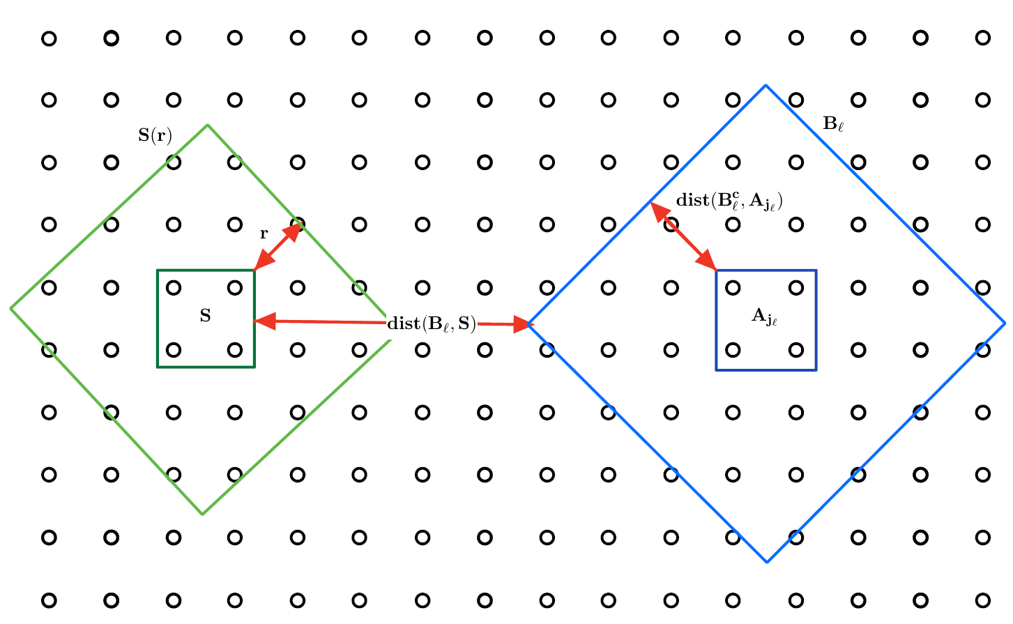
Figure 1: Diagram showing the regions involved in the proof Lemma C.5.

By construction, for $r>2r_{0}$, the condition that $A_{j_{l}}\cap S=\emptyset$ is met, and therefore the bound holds. We recall that $i\in\Lambda$ is defined as the center of $S$. Since $\operatorname{dist}(i,j_{l})=k_{0}/2+\operatorname{dist}(S,B_{l})+\operatorname{dist}(A_{j_{l}},B_{l})+r_{0}$, we can choose $B_{l}$ so that $\operatorname{dist}(S,B_{l}),\operatorname{dist}(A_{j_{l}},B_{l})\geq\operatorname{dist}(i,j_{l})/2-k_{0}/4-r_{0}/2-1$. Therefore,

$$\operatorname{Cov}_{\sigma(\beta,x)}(O,\,\widetilde{H}_{l}(x))\leq 4(C+c^{\prime})C^{\prime\prime}\|O\|_{\infty}(2r_{0}+k_{0})^{D}\,he^{-\operatorname{dist}(i,j_{l})/\xi}$$

where $1/\xi=\min\{\mu^{\prime},\nu\}$ and $C^{\prime\prime}:=e^{\max\{\mu^{\prime},\nu\}(k_{0}/4+r_{0}/2+1)}$. Therefore

$$|f_{O}(x)-f_{O}(x|_{\mathcal{S}_{i}(r)})| \leq 4\beta(C+c^{\prime})\,h\,(2r_{0}+k_{0})^{D}\,\|O\|_{\infty}\sum_{l\in\mathcal{S}(r)^{c}}\,e^{-\operatorname{dist}(i,j_{l})/\xi}\,.$$

Upon shifting the center of the lattice at site $i$, we get

$$|f_{O}(x)-f_{O}(x|_{\mathcal{S}(r)})| \leq 4\beta(C+c^{\prime})C^{\prime\prime}\,h\,(2r_{0}+k_{0})^{D}\,\|O\|_{\infty}\sum_{|l|\geq r+k_{0}/2}\,e^{-|l|/\xi}$$

$$=4\beta(C+c^{\prime})C^{\prime\prime}\,h\,(2r_{0}+k_{0})^{D}\,\|O\|_{\infty}\sum_{a>r+k_{0}/2}\,\binom{a+D-1}{D-1}\,e^{-a/\xi}$$

$$\leq 4\beta(C+c^{\prime})C^{\prime\prime}\,h\,(2r_{0}+k_{0})^{D}\,D^{D-1}\|O\|_{\infty}\sum_{a>r+k_{0}/2}\,a^{D-1}\,e^{-a/\xi}$$

$$\leq 4\beta(C+c^{\prime})C^{\prime\prime}\,h\,(2r_{0}+k_{0})^{D}(D-1)!(2\xi)^{D-1}\,D^{D-1}\|O\|_{\infty}\sum_{a>r+k_{0}/2}\,\,e^{-\frac{a}{2\xi}}$$

$$\leq 4\beta(C+c^{\prime})C^{\prime\prime}\,h\,(2r_{0}+k_{0})^{D}(D-1)!(2\xi)^{D-1}\,D^{D-1}\|O\|_{\infty}\,\frac{e^{-\frac{r+k_{0}/2+1}{2\xi}}}{1-e^{-\frac{1}{2\xi}}}$$

$$\equiv C_{1}\,e^{-\frac{r}{2\xi}}\,\|O\|_{\infty}\,,$$

where $C_{1}$ depends upon all the parameters of the problem.

∎

In the case when we are interested in distinguishing two Gibbs states with Lipschitz observables, over extended subregions of the lattice, the following extension of Corollary C.4 can be easily shown to hold:

Corollary C.6.

Assume that the states $\sigma(\beta,x)$ satisfy the condition of decay of correlations A.1. Then for any region $S$ of the lattice and any two $x,y\in[-1,1]^{m}$

$$W_{1}(\operatorname{tr}_{S^{c}}(\sigma(\beta,x)),\operatorname{tr}_{S^{c}}(\sigma(\beta,y)))\leq\|x|_{\mathcal{S}(r)}-y|_{\mathcal{S}(r)}\|_{\ell_{1}}\,\operatorname{polylog}(|S(r)|)\,,$$

where $r=\max\Big{\{}r_{0},\,2\xi\log\Big{(}\frac{2|S|C_{1}}{\|x|_{\mathcal{S}(r_{0})}-y|_{\mathcal{S}(r_{0})}\|_{\ell_{1}}}\Big{)}\Big{\}}$ with $r_{0}$ being the smallest integer such that $x|_{\mathcal{S}(r_{0})}\neq y|_{\mathcal{S}(r_{0})}$, and $C_{1},\xi$ are the same constants as in Lemma C.5.

Proof.

Given $L_{S}$ a Lipchitz observable supported on region $S$ of the lattice, we have for any $r\in\mathbb{N}$:

$$\big{|}f_{L_{S}}(x)-f_{L_{S}}(y)\big{|} \leq\|L_{S}\|_{\infty}\,\Big{(}\big{\|}\operatorname{tr}_{S^{c}}\big{(}\sigma(\beta,x)-\sigma(\beta,x|_{\mathcal{S}(r)})\big{)}\big{\|}_{1}+\big{\|}\operatorname{tr}_{S^{c}}\big{(}\sigma(\beta,y)-\sigma(\beta,y|_{\mathcal{S}(r)})\big{)}\big{\|}_{1}\Big{)}$$

$$\qquad+W_{1}\big{(}\sigma(\beta,x|_{\mathcal{S}(r)}),\sigma(\beta,y|_{\mathcal{S}(r)})\big{)}$$

$$\leq 2\,|S|\,\|L_{S}\|_{\operatorname{Lip}}\,C_{1}\,e^{-\frac{r}{2\xi}}+W_{1}\big{(}\sigma(\beta,x|_{\mathcal{S}(r)}),\sigma(\beta,y|_{\mathcal{S}(r)})\big{)}\,,$$

where the second line follows from Equation C.16. By Corollary C.4, we conclude that

$$W_{1}\big{(}\operatorname{tr}_{S^{c}}(\sigma(\beta,x)),\operatorname{tr}_{S^{c}}(\sigma(\beta,y))\big{)} \leq 2\,|S|\,C_{1}\,e^{-\frac{r}{2\xi}}+W_{1}\big{(}\sigma(\beta,x|_{\mathcal{S}(r)}),\sigma(\beta,y|_{\mathcal{S}(r)})\big{)}$$

$$\leq 2\,|S|\,C_{1}\,e^{-\frac{r}{2\xi}}+\|x|_{\mathcal{S}(r)}-y|_{\mathcal{S}(r)}\|_{\ell_{1}}\,\operatorname{polylog}(|S(r)|)\,.$$

Next, we choose $r=2\xi\log\Big{(}\frac{2|S|C_{1}}{\|x|_{\mathcal{S}(r_{0})}-y|_{\mathcal{S}(r_{0})}\|_{\ell_{1}}}\Big{)}$, where $r_{0}$ is the smallest integer such that $x|_{\mathcal{S}(r_{0})}\neq y|_{\mathcal{S}(r_{0})}$. ∎

C.3 Gibbs state tomography beyond the trivial phase

All of the results discussed so far in this section concerned parametrized families of Gibbs states that included the maximally mixed state. Let us now discuss to what extent our results generalize to the setting of where we add a fixed Hamiltonian term $H_{0}$, as discussed around Eq. (A.2). As made explicit in the proof of Corollary C.4, the main technical result required for the continuity of $W_{1}$ w.r.t. the parameters is a bound on the derivative $|\partial_{x^{\prime}_{k}}f_{L}(\beta,x)|$ in terms of the Lipschitz constant we obtained in Proposition C.3. In turn, to prove those bounds, the main technical assumptions we required were exponential decay of correlations and the existence of LR bounds. We then have:

Corollary C.7.

Assume that $\sigma(\beta,x,H_{0})$ satisfies the condition of decay of correlations, A.1 and that the time evolution defined by the Hamiltonian $H(x)+H_{0}$ satisfies a LR-bound as in Equation C.6. Define the function $f_{L,H_{0}}(\beta,x)=\operatorname{tr}[L\sigma(x,\beta,H_{0})]$. Then for any $k\in[m]$,

$$|\partial_{x^{\prime}_{k}}f_{L,H_{0}}(\beta,x)|\leq\,\|L\|_{\operatorname{Lip}}\,\operatorname{polylog}(n)\,,$$ (C.18)

for some polynomial of $\log(n)$ of degree $D$ with coefficients depending on $\beta,r_{0},D,h,c^{\prime},\nu,\mu^{\prime}$ and $C$. In particular, it follows that

$$W_{1}(\sigma(\beta,x,H_{0}),\sigma(\beta,y,H_{0}))\leq\,\|x-y\|_{\ell_{1}}\,\operatorname{polylog}(n)\,.$$ (C.19)

Proof.

How Equation C.19 follows from Equation C.18 is completely equivalent to Corollary C.4. To obtain the inequality in Equation C.18 we use the fact that

$$\partial_{x^{\prime}_{k}}f_{L,H_{0}}(\beta,x)=-\frac{\beta}{2}\,\operatorname{tr}\Big{[}L\big{\{}\Phi_{H(x)+H_{0}}(\partial_{x^{\prime}_{k}}(H(x))),\sigma(\beta,x,H_{0})\big{\}}\Big{]}+$$

$$\beta\operatorname{tr}(\partial_{x^{\prime}_{k}}(H(x))\sigma(\beta,x,H_{0}))\,\operatorname{tr}(L\sigma(\beta,x,H_{0}))\,.$$

A close inspection of the proof of Proposition C.3 shows that all that was required to then bound the derivative was a LR-bound and the exponential decay of correlations, which we assume to also be given in this setting. ∎

The other results of the previous section also generalize to our setting with constant shift $H_{0}$, but we will not state them explicitly for the sake of conciseness.

C.4 Hamiltonian estimation and optimal Gibbs state tomography

From Corollary C.4 it is immediate that we reduced the problem of obtaining a good estimate in $W_{1}$ to the problem of estimating the parameters of the Gibbs state $\sigma(\beta,x)$. Indeed, it is clear that if we can obtain an estimate $x^{\prime}$ of $x$ satisfying

$$\|x-x^{\prime}\|_{\ell_{1}}=\mathcal{O}(\varepsilon n/\textrm{polylog}(n)),$$ (C.20)

then it suffices to ensure that $W_{1}(\sigma(\beta,x),\sigma(\beta,x^{\prime}))=\varepsilon n$. Let us discuss some examples where we can obtain this efficiently with $\mathcal{O}(\varepsilon^{-2}\textrm{polylog}(n))$ samples.

C.4.1 Commuting Hamiltonians

In [4], the authors give an algorithm which with

$$e^{\mathcal{O}(\beta k^{D})}\mathcal{O}(\log(\delta^{-1}n)\varepsilon^{-2})$$ (C.21)

copies of $\sigma(\beta,x)$ learns $x$ up to $\varepsilon$ in $\ell_{\infty}$ distance when $\sigma(\beta,x)$ belongs to a family of commuting, $k$-local Hamiltonians on a $D$-dimensional lattice. As we assumed that the number of parameters $m=\mathcal{O}(n)$, this translates to an algorithm with sample complexity $e^{\mathcal{O}(\beta k^{D})}\mathcal{O}(\varepsilon^{-2}\textrm{polylog}(\delta^{-1}n))$ to learn $x$ up to $\varepsilon n$ in $\ell_{1}$ distance. It should be noted that the time complexity of their algorithm is $\mathcal{O}(ne^{\mathcal{O}(\beta k^{D})}\varepsilon^{-2}\textrm{polylog}(\delta^{-1}n))$.

Thus, any commuting model at constant temperature satisfying exponential decay of correlations can be efficiently learned with $\operatorname{polylog}(n)$ samples. Examples of classes of commuting states that satisfy exponential decay of correlations include:

1. $1$D translation-invariant Hamiltonians at any positive temperature [5].

2. Commuting Gibbs states of Hamiltonians on regular lattices below a threshold temperature [53, 44].

3. Classical spin models away from criticality [33, 61, 44].

4. Ground states of gapped systems [16, 14, 63, 64].

C.4.2 High-temperature Gibbs states

Another class of states for which the conditions of our results hold are local Gibbs states on a lattice above a threshold temperature that depends on the locality of the Hamiltonian and the dimension of the lattice. These systems are known to have exponential decay of correlations [53, 44]. Furthermore, in [42] the authors give an algorithm to learn $x$ up to error $\varepsilon$ in $\ell_{\infty}$ norm from $\mathcal{O}(\varepsilon^{-2}\textrm{polylog}(\delta^{-1}n))$ samples. This again translates to a $\mathcal{O}(\varepsilon n)$ error in $\ell_{1}$ norm. Note that their algorithm also is computationally efficient.

We note that in [1] the authors give an algorithm to learn the Hamiltonian of any Gibbs state of positive temperature through the maximum entropy method. However, their results require a polynomial number of samples to recover the parameters in $\ell_{1}$ distance. Thus, their results do not work for the polylog regime investigated in this work.

C.4.3 Gibbs state of exponentially decaying correlations and conditional mutual information

In the previous section, we extracted two regimes for which there exist efficient Gibbs tomography algorithms from previous works, namely the commuting and the high-temperature regimes. As said before, depending on the Hamiltonian, exponential decay of correlations can also occur in the low-temperature regime, and it is an interesting open question whether our strategy can be adapted to that setting for non-commuting interactions.

Here, we show that the Gibbs state $\sigma(\beta,x)$ of a possibly non-commuting Hamiltonian $H(x)$ can also be estimated in Wasserstein distance up to multiplicative error $\varepsilon n$ given $\operatorname{polylog}(n)$ copies of it as long as the latter has exponentially decaying correlations and is close to a quantum Markov chain, hence partially answering an open problem previously raised in [1].

To be more precise, in this section we will require a stronger notion of decay of correlations.

Definition C.8 (Uniform clustering).

The Gibbs state $\sigma(\beta,x)$ is said to be uniformly $\zeta(\ell)$-clustering if for any $X\subset\Lambda$ and any $A\subset X$ and $B\subset X$ such that $\operatorname{dist}(A,B)\geq\ell$,

$$\operatorname{Cov}_{\sigma(\beta,x,X)}(X_{A},X_{B})\leq\|X_{A}\|_{\infty}\,\|X_{B}\|_{\infty}\,\zeta(\ell)$$

for any $X_{A}$ supported on $A$ and $X_{B}$ supported on $B$.

As pointed out in [18], this property is called uniform clustering to contrast with regular clustering property that usually only refers to properties of the state $\sigma(\beta,x)$.

Definition C.9 (Uniform Markov condition).

The Gibbs state $\sigma_{\beta}(x)$ is said to satisfy the uniform $\delta(\ell)$-Markov condition if for any $ABC=X\subset\Lambda$ with $B$ shielding $A$ away from $C$ and such that $\operatorname{dist}(i,j)\geq\ell$ for any $i\in A$ and $j\in C$, we have

$$I(A:C|B)_{\sigma(\beta,x,X)}\leq\delta(\ell)\,.$$

This property always holds for commuting Gibbs states for a function $\delta(\ell)=0$ as soon as $\ell$ is larger than twice the interaction range. Although not proven yet, it is believed that the approximate Markov property holds with some generality for non-commuting Gibbs states. The 1D and high-temperature settings were investigated in [51] and [55], respectively. The decay of the conditional mutual information was also shown for finite temperature Gibbs states of free fermions, free bosons, conformal field theories, and holographic models [80], as well as more recently for purely generated finitely correlated states in [78].

We will now show how to learn states that satisfy both the uniform Markov condition and the uniform clustering of correlations. Our strategy consists in using the maximum entropy estimation [48, 47, 49, 19], already appearing in [1], to construct an estimator $\hat{x}$ of the parameter $x\in[-1,1]^{m}$. The condition of exponential decay of correlations and that of approximate Markov chain will ensure that $W_{1}(\sigma(\beta,\hat{x}),\sigma(\beta,x))=o(n)$. Thus, we once again emphasise that our goal is to obtain a good recovery of the state, not of the parameter $x$.

For sake of clarity and simplicity of presentation, we only consider the $1$D setting, although our method easily extends to arbitrary dimension. We assume that each interaction $h_{j}(x_{j})$ is of the form

$$h_{j}(x_{j}):=\sum_{l=1}^{\ell}x_{j,l}\,h_{j,l}$$

for some self-adjoint operators $h_{j,l}$ supported in $A_{j}:=\{k\in\Lambda|\operatorname{dist}(k,j)\leq r_{0}\}$ with $\|h_{j,l}\|\leq h$, where we denoted by $x_{j,l}$ the entries of $x_{k}$. We also recall that given a region $R$ of the lattice, we denote $H_{R}(x):=\sum_{k\in R}h_{k}(x_{k})$. In what follows, with a slight abuse of notations, we denote by the same symbol a vector $y=\{y_{k,l}\}_{k\in N_{j}}$ and its embedding $(y,0)$ onto $[-1,1]^{m}$. Then, given an inverse temperature $\beta>0$, we define the partition function as

$$Z_{\beta}(x)=\operatorname{tr}\big{[}e^{-\beta H(x)}\big{]}\,.$$

The maximum entropy problem consists in the following strongly convex optimisation problem.

Theorem C.10 ([1]).

Given an unknown Hamiltonian $H(x)=\sum h_{j}(x_{j})$, define $e_{k,l}=\operatorname{tr}[h_{k,\ell}\sigma(\beta,x)]$. Solving the following optimisation problem:

$$\hat{x}:=\underset{y\in[-1,1]^{m}}{\operatorname{arg\leavevmode\nobreak\ min}}\,L(y)\,,\qquad\text{ where }\qquad L(y):=\log Z_{\beta}(y)+\beta\sum_{k\in\Lambda}\sum_{l=1}^{\ell}y_{k,l}\,e_{k,l}\,$$ (C.22)

gives $\hat{x}$ such that $\sigma(\beta,\hat{x})=\sigma(\beta,x)$.

In an experimental setting, we will not have access to the exact $\{e_{k,l}\}_{k,l}$, but instead may be able to approximate them using by having access to the state. However, we want to be sure that having a reasonably good approximation to $e_{k,l}$ is sufficient to approximate $x$. To do so one can make use of the fact that

$$\log Z_{\beta}(\hat{x})\leq\log Z_{\beta}(x)+\beta\sum_{k\in\Lambda}\sum_{l=1}^{\ell}\,(x_{k,l}-\hat{x}_{k,l})\,\widetilde{e}_{k,l}\,.$$ (C.23)

Further assuming $\alpha_{2}$ is a lower bound on the strong convexity constant associated to the function $x\mapsto\log Z_{\beta}(x)$, that is $\nabla^{2}Z_{\beta}\geq\alpha_{2}\,I$, we have by Taylor expansion and since $\partial_{x_{k,l}}\log Z_{\beta}(x)=-\beta e_{k,l}(x)$:

$$\log Z_{\beta}(\hat{x})\geq\log Z_{\beta}(x)-\beta\sum_{k\in\Lambda}\sum_{l=1}^{\ell}\,(\hat{x}_{k,l}-x_{k,l})\,e_{k,l}(x)+\frac{\alpha_{2}}{2}\,\|x-\hat{x}\|_{\ell_{2}}^{2}\,.$$ (C.24)

Combining the two bounds above, we find that

$$\|x-\hat{x}\|_{\ell_{2}}^{2}\leq\frac{2\beta}{\alpha_{2}}\,\sum_{k,l}(x_{k,l}-\hat{x}_{k,l})(\widetilde{e}_{k,l}-e_{k,l}(x))\leq\frac{2\beta}{\alpha_{2}}\,\|x-\hat{x}\|_{\ell_{2}}\,\|e-\widetilde{e}\|_{\ell_{2}}\,,$$

and hence $\|x-\hat{x}\|_{\ell_{2}}\leq\frac{2\beta\sqrt{\ell|\Lambda|}\,\eta}{\alpha_{2}}$, thus giving the following theorem:

Theorem C.11 ([1]).

Suppose $\widetilde{e}_{k,l}$ is an approximation of $e_{k,l}(x):=\operatorname{tr}\big{[}h_{k,l}\,\sigma(\beta,x)\big{]}$ with $\|\widetilde{e}-e(x)\|_{\ell_{\infty}}\leq\eta$. Assume that the following inequality is satisfied for some $\alpha_{2}$: $\nabla^{2}Z_{\beta}\geq\alpha I$. Solving the following optimisation problem:

$$\hat{x}:=\underset{y\in[-1,1]^{m}}{\operatorname{arg\leavevmode\nobreak\ min}}\,L(y)\,,\qquad\text{ where }\qquad L(y):=\log Z_{\beta}(y)+\beta\sum_{k\in\Lambda}\sum_{l=1}^{\ell}y_{k,l}\,\widetilde{e}_{k,l}\,$$ (C.25)

gives an output $\hat{x}$ satisfying:

$$\left\lVert\hat{x}-x\right\rVert_{\ell_{2}}\leq\frac{2\beta\eta\sqrt{\ell\Lambda}}{\alpha_{2}}.$$

Using the bound on $\hat{x}$ from Theorem C.11 the equivalence between $\ell_{1}$ and $\ell_{2}$-norms, we have that

$$\|x-\hat{x}\|_{\ell_{1}}\leq\frac{2\beta\ell n\eta}{\alpha_{2}}\,,$$

which provides us with the right scaling for our $\ell_{1}$ approximation problem as long as $\eta=o(1)$ and $\alpha_{2}=\Omega(1)$. Unfortunately, the constant $\alpha_{2}$ could only be proved to scale inverse polynomially with $n$ in [1]. A first idea from there is to try and find a constant $\alpha_{1}=\Omega(n^{-1})$ such that the following strong convexity bound with respect to the $\ell_{1}$-norm holds. As per eq. C.24, this would imply:

$$\log Z_{\beta}(\hat{x})\geq\log Z_{\beta}(x)-\beta\sum_{k,l}(\hat{x}_{k,l}-x_{k,l})\,e_{k,l}(x)+\frac{\alpha_{1}}{2}\,\|x-\hat{x}\|_{\ell_{1}}^{2}\,.$$ (C.26)

If such a bound held, we would conclude similarly to the previous setting that

$$\|x-\hat{x}\|_{\ell_{1}}\leq\frac{2\beta\eta}{\alpha_{1}}=o(\eta n)\,.$$

Which together with the continuity bound Equation C.9 would allow us to get the desired recovery estimate in Wasserstein distance. Now, it can be seen that Equation C.26 is equivalent to

$$\|x-\hat{x}\|_{\ell_{1}}^{2}\leq\,\frac{2}{\alpha_{1}}\,D(\sigma(\beta,x)\|\sigma(\beta,\hat{x}))\,.$$ (C.27)

Here we recall that the relative entropy between two quantum states $\rho$ and $\sigma$ with $\operatorname{supp}(\rho)\subseteq\operatorname{supp}(\sigma)$ is $D(\rho\|\sigma):=\operatorname{tr}\rho\log\rho-\operatorname{tr}\rho\log\sigma$. This together with Equation C.9 would lead to the following local version of the transportation cost inequality

$$W_{1}(\sigma(\beta,x),\sigma(\beta,\hat{x}))^{2}\leq\mathcal{O}(n\operatorname{polylog}(n))\,D(\sigma(\beta,x)\|\sigma(\beta,\hat{x}))\,.$$ (C.28)

In [70], such inequality was shown to hold in the high-temperature regime only for commuting $H$, albeit when $\sigma(\beta,x)$ can be replaced by an arbitrary state $\rho$ on the lattice. The latter is referred to as a transportation-cost inequality for the state $\sigma(\beta,\hat{x})$. Since Equation C.26 consists in a strengthening of Equation C.28, proving it directly appears difficult. Here instead, we want to show the following weakening of (C.28):

$$W_{1}(\sigma(\beta,x),\sigma(\beta,\hat{x}))^{2}\leq\mathcal{O}(n\operatorname{polylog}(n))\,D(\sigma(\beta,x)\|\sigma(\beta,\hat{x}))\,+o(\varepsilon n)\,,$$

for some constant $\delta$ which depends on the approximate Markov as well as the correlation decay properties of the Gibbs state $\sigma(\beta,\hat{x})$. More precisely, we show the following extension of [70, Theorem 4] to Gibbs states of non-commuting Hamiltonians.

Proposition C.12 (Generalised transportation-cost inequality).

With the notations of the above paragraph, for all states $\rho$:

$$W_{1}(\rho,\sigma(\beta,x))\,\leq\,\inf_{\ell\in\mathbb{N}}\mathcal{O}(\ell\sqrt{n})\,\sqrt{D(\rho\|\sigma(\beta,x))}+n^{2}\big{(}\delta(\mathcal{O}(\ell))+\zeta(\mathcal{O}(\ell))+e^{-\mathcal{O}(\ell)}\big{)}\,.$$

In particular, if both $\zeta(l),\delta(l)=\mathcal{O}(e^{-\xi l})$, then for $l=\mathcal{O}(\xi^{-1}\log(n\varepsilon^{-1}))$ we have

$$W_{1}(\rho,\sigma(\beta,x))\,\leq\,\mathcal{O}(\log(n\varepsilon^{-1})\sqrt{n})\,\sqrt{D(\rho\|\sigma(\beta,x))}+o(\varepsilon n).$$ (C.29)

Proof.

The proof is adapted from that of [70, Theorem 4]. We first consider a bipartite quantum subsystem $AB\subset\Lambda$ and a joint quantum state $\omega_{AB}$ of $AB$. We then define the so-called quantum recovery map [76, 50] by its action on a quantum state $\rho_{A}$ on region $A$:

$$\Phi_{A\to AB}(\rho_{A})=\int_{\mathbb{R}}\omega_{AB}^{\frac{1-it}{2}}\,\omega_{A}^{\frac{it-1}{2}}\,\rho_{A}\,\omega_{A}^{-\frac{1+it}{2}}\,\omega_{AB}^{\frac{1+it}{2}}\,d\mu_{0}(t)\,,$$ (C.30)

where $\mu_{0}$ is the probability distribution on $\mathbb{R}$ with density

$$d\mu_{0}(t)=\frac{\pi\,dt}{2\left(\cosh(\pi t)+1\right)}\,.$$ (C.31)

If $A$ is in the state $\omega_{A}$, the recovery map $\Phi_{A\to AB}$ recovers the joint state $\omega_{AB}$, i.e., $\Phi_{A\to AB}(\omega_{A})=\omega_{AB}$. The relevance of the recovery map comes from the recoverability theorem [76], which states that $\Phi_{A\to AB}$ can recover a generic joint state $\rho_{AB}$ from its marginal $\rho_{A}$ if removing the subsystem $B$ does not significantly decrease the relative entropy between $\rho$ and $\omega$. More precisely, for any quantum state $\sigma_{AB}$ of $AB$ we have

$$D(\sigma_{AB}\|\omega_{AB})-D(\sigma_{A}\|\omega_{A})\geq D_{\mathbb{M}}(\sigma_{AB}\|\Phi_{A\to AB}(\sigma_{A}))\,,$$ (C.32)

where $D_{\mathbb{M}}$ denotes the measured relative entropy [30, 67, 45, 11]

$$D_{\mathbb{M}}(\sigma\|\omega):=\sup_{(\mathcal{X},M)}\,D(P_{\sigma,M}\|P_{\omega,M})\,,$$ (C.33)

where the supremum above is over all positive operator valued measures $M$ that map the input quantum state to a probability distribution on a finite set $\mathcal{X}$ with probability mass function given by $P_{\rho,M}(x)=\operatorname{tr}\rho M(x)$.

Next, we split region $A$ into regions $A_{1}$ and $A_{2}$ such that $A_{1}$ shields $A_{2}$ away from $B$, and take $\sigma_{AB}:=\operatorname{tr}_{(AB)^{c}}(\sigma(\beta,x))$ and $\omega_{AB}=\sigma_{A_{1}B}\otimes\sigma_{A_{2}}$ In that case, (C.32) becomes

$$I(B:A_{2}|A_{1})_{\sigma}\geq D_{\mathbb{M}}\big{(}\sigma\|\Phi_{A_{1}\to A_{1}B}(\sigma_{A})\big{)}\,,$$ (C.34)

where we also used that the state $\omega$ is a tensor product in the cut $A_{1}B-A_{2}$, so that $\Phi_{A\to B}=\Phi_{A_{1}\to B}$.

Next, we pave the chain $\Lambda$ into unions of intervals $A=\cup_{i=1}^{M}A_{i}$ and $B=\cup_{i=1}^{M}B_{i}$ such that $A_{i}\cap B_{i}\neq\emptyset$ and $B_{i}\cap A_{i+1}\neq\emptyset$. As in [18], we then define the channel $\mathcal{F}:=\mathcal{F}_{A}\circ\mathcal{F}_{B}$ where $\mathcal{F}_{B}:=\bigotimes_{i}\sigma(\beta,x,B_{i})\otimes\operatorname{tr}_{B_{i}}$ and $\mathcal{F}_{A}:=\prod_{j}\Phi_{A_{i}\backslash B\to A_{i}}\circ\operatorname{tr}_{A_{i}}$. In words, the channel $\mathcal{F}_{B}$ first prepares the Gibbs state in the region $B$, whereas $\mathcal{F}_{A}$ prepares the remaining of the Gibbs state onto region $A\backslash B$. Then, we have, for any state $\rho$

$$W_{1}(\rho,\sigma(\beta,x)) \leq W_{1}(\rho,\mathcal{F}_{B}(\rho))+W_{1}(\mathcal{F}_{B}(\rho),\mathcal{F}_{A}\circ\mathcal{F}_{B}(\rho))+W_{1}(\mathcal{F}(\rho),\sigma(\beta,x))$$

$$\leq\sum_{i}W_{1}(\sigma(A,i),\sigma(A,i+1))+\sum_{i}\,W_{1}(\sigma(B,i),\sigma(B,i+1))+n\,\|\mathcal{F}(\rho)-\sigma(\beta,x)\|_{1}$$

$$\overset{(1)}{\leq}R\,\sum_{i}\,\|\sigma(A,i)-\sigma(A,i+1)\|_{1}+\|\sigma(B,i)-\sigma(B,i+1)\|_{1}+n\|\mathcal{F}(\rho)-\sigma(\beta,x)\|_{1}\,,$$

where $\sigma(A,i):=\bigotimes_{j<i}\sigma(\beta,x,B_{j})\otimes\operatorname{tr}_{B_{j}}(\rho)$ and $\sigma(B,i):=\bigotimes_{j<i}\Phi_{A_{j}\backslash B,\to A_{j}}\circ\operatorname{tr}_{A_{j}}(\mathcal{F}_{B}(\rho))$, and where $R=\max\{|B_{i}|,|A_{i}|\}$ so that $(1)$ follows from [31, Propositiom 5]. Next, we use Pinsker’s inequality, so

$$W_{1}(\rho,\sigma(\beta,x))$$

$$\qquad\leq R\sqrt{2}\,\sum_{i}\sqrt{D_{\mathbb{M}}(\sigma(A,i)\|\sigma(A,i+1))}+\sqrt{D_{\mathbb{M}}(\sigma(B,i)\|\sigma(B,i+1))}\,+n\,\|\mathcal{F}(\rho)-\sigma(\beta,x)\|_{1}$$

$$\qquad\leq 2R\sqrt{M}\,\left(\sum_{i}D_{\mathbb{M}}(\sigma(A,i)\|\sigma(A,i+1))+D_{\mathbb{M}}(\sigma(B,i)\|\sigma(B,i+1))\right)^{\frac{1}{2}}+n\|\mathcal{F}(\rho)-\sigma(\beta,x)\|_{1}$$

$$\qquad\overset{(1)}{\leq}2R\sqrt{M}\,\sqrt{D(\rho\|\sigma(\beta,x))}+n\|\mathcal{F}(\rho)-\sigma(\beta,x)\|_{1}$$

$$\qquad\overset{(2)}{\leq}2R\sqrt{M}\,\sqrt{D(\rho\|\sigma(\beta,x))}+n^{2}\big{(}\delta(\mathcal{O}(R))+\zeta(\mathcal{O}(R))+C_{1}e^{-c_{2}R}\big{)}\,,$$

where $(1)$ follows from multiple uses of (C.32) as well as the sub-additivity of the relative entropy under tensor products in its second argument, whereas $(2)$ comes from [18, Theorem 6]. The result follows. ∎

We can then easily turn the previous statement into one about learning the state $\sigma(\beta,x)$:

Corollary C.13 ($W_{1}$ learning from the uniform Markov condition).

Under the same conditions of Proposition C.12 assume further that $\zeta(l),\delta(l)=\mathcal{O}(e^{-\xi l})$. Then $\mathcal{O}(\varepsilon^{-4}\operatorname{polylog}(n\delta^{-1}))$ samples of $\sigma(\beta,x)$ suffice to learn a state $\sigma(\beta,x^{\prime})$ s.t. with probability at least $1-\delta$

$$W_{1}(\sigma(\beta,x),\sigma(\beta,x^{\prime}))=\mathcal{O}(\varepsilon n).$$ (C.35)

Proof.

We simply need to adapt the proof of Equation C.27. First, we recall that

$$D(\sigma(\beta,x)\|\sigma(\beta,\hat{x}))=\beta\sum_{k,l}(\hat{x}_{k,l}-x_{k,l})\,e_{k,l}(x)+\log Z_{\beta}(\hat{x})-\log Z_{\beta}(x)\,.$$

Together with Equation C.29, we have the following approximate strong convexity bound for the log partition function in the Wasserstein topology:

$$W_{1}(\sigma(\beta,x),\sigma(\beta,\hat{x}))^{2}\leq\mathcal{O}(\log(n\varepsilon^{-1})^{2}{n})\,D(\rho\|\sigma(\beta,x))+o(\varepsilon^{2}n^{2})$$

Combining with Equation C.23 and assuming that $\|\widetilde{e}-e(x)\|_{\ell_{\infty}}\leq\eta$, we get

$$W_{1}(\sigma(\beta,x),\sigma(\beta,\hat{x}))^{2} \leq\mathcal{O}(\log(n\varepsilon^{-1})^{2}{n})\,\beta\,\sum_{k,l}(\hat{x}_{k,l}-x_{k,l})(e_{k,l}(x)-\widetilde{e}_{k,l})+o(\varepsilon^{2}n^{2})$$

$$\leq\mathcal{O}(\log(n\varepsilon^{-1})^{2}{n^{2}})\,\eta\,+o(\varepsilon^{2}n^{2})\,.$$

Above, we have managed to reduce the problem to that estimating the coefficients $e_{k,l}$ to precision $\eta=\mathcal{O}(\varepsilon^{2}/\operatorname{polylog}(n))$. This can be done with probability $1-\delta$ given $\mathcal{O}(\varepsilon^{-4}\operatorname{polylog}(n\delta^{-1}))$ copies of the state $\sigma(\beta,x)$ through various methods (see e.g. [73, Appendix A] or [1, Corrolary 27] for more details).

∎

Remark C.14.

The main difference between the approach outlined in the proposition above and that of Corollary C.4 is that, besides requiring the additional assumption of uniform Markovianity, it has an $\varepsilon^{-4}$ scaling with the precision instead of $\varepsilon^{-2}$. However, it completely bypasses the need for a good algorithm to learn the parameters $x$, which is required to apply Corollary C.4. Indeed, note that all that was required was to find another Gibbs state that approximates the local expectation values $e_{k,l}(x)$, which can be achieved through the maximum entropy principle. However, to the best of our knowledge, it is not known how to run the maximum entropy principle efficiently for the classes of states considered in Corollary C.4 on a classical computer. On the other hand, the results of [18] show that we can run maximum entropy efficiently for the states under consideration for Corollary C.4 on a quantum computer.

Conversely, if combined with an $\ell_{2}$ strong convexity guarantee on the partition function, the $\varepsilon^{-2}$ scaling can be recovered (see e.g. [73, Theorem A.1] for more details). But, since we are currently only able to get this guarantee for commuting Hamiltonians or in the high-temperature regimes, Corollary C.4 provides a more direct path than the strategy previously exhibited in [73].

Appendix D Algorithm for learning observables in high temperature phases

Next, we assume we are given different Gibbs states $\sigma(\beta,x)$ where $x$ is sampled according to the uniform distribution $U$ over $x\in[-1,1]^{m}$, and wish to learn the expectation value of an unknown observable for all values of $x\in[-1,1]^{m}$. We assume that the Gibbs states in the interval $[-1,1]^{m}$ has exponentially decaying correlations everywhere, which can be thought of as defining a continuous phase of matter. For commuting Hamiltonians, this relationship can be made more precise [44].

As before, for pedagogical reasons we will first solve this problem for phases that contain the maximally mixed state in them and, thus, we can compute local expectations efficiently on a classical computer. But then we will show how these results easily generalize to phases that are more computationally involved by once again shifting the center of the phase. We will discuss these more involved examples in Appendix E.

During a training stage, we pick $N$ points $Y_{1},\dots,Y_{N}\sim U$ independently distributed uniformly at random in $[-1,1]^{m}$ and are given access to the Gibbs states $\sigma(\beta,Y_{j})$. Next, fix $r\in\mathbb{N}$. Given an observable $O=\sum_{i=1}^{M}O_{i}$, we define $S_{i}=\operatorname{supp}(O_{i})$ and for each $S_{i}$ there is a ball of diameter at most $k_{0}$ containing $S_{i}$, and $S_{i}(r):=\{j\in\Lambda|\operatorname{dist}(j,S_{i})\leq r\}$. We construct for any $x\in[-1,1]^{m}$ the estimator

$$\hat{f}_{O}(x)=\sum_{i=1}^{M}\operatorname{tr}\big{[}O_{i}\,\sigma(\beta,\hat{Y}_{i}(x))\big{]}\,,\quad\text{ with }\quad\hat{Y}_{i}(x)=\operatorname{argmin}_{{Y}_{k}}\|x|_{\mathcal{S}_{i}(r)}-{Y}_{k}|_{\mathcal{S}_{i}(r)}\|_{\ell^{\infty}}\,,$$ (D.1)

where we recall that we denote by $x_{\mathcal{S}_{i}(r)}$ the concatenation of vectors $x_{j}$ corresponding to interactions $h_{j}$ supported on regions intersecting $S_{i}(r)$. In words, we approximate the expectation value of $O_{i}$ by that of the Gibbs state whose parameters in a region around $S_{i}$ are the closest to the state of interest. We also denote $\mathcal{S}_{i}\equiv\mathcal{S}_{i}(0)$.

Lemma C.5 demonstrates that to measure a particular observable, it is sufficient to consider the parameters only spatially local to it. One important technical tool for that is the following Lemma from [22]:

Lemma D.1 (Lemma 16 of  [22]).

Let $H,H^{\prime}$ be Hermitian matrices. Then:

$$\Big{\|}\frac{e^{-H_{1}}}{\operatorname{tr}\left[e^{-H_{1}}\right]}-\frac{e^{-H_{2}}}{\operatorname{tr}\left[e^{-H_{2}}\right]}\Big{\|}\leq 2(e^{\|H_{1}-H_{2}\|_{\infty}}-1).$$ (D.2)

Next, we show that if we are given a number of samples uniformly sampled from $[-1,1]^{m}$, we can construct an estimator for the observable to high precision.

Proposition D.2.

Assuming the exponential decay of correlations in A.1, the estimator $\hat{f}_{O}(x):=\sum_{i}\,\operatorname{tr}[O_{i}\,\sigma(\beta,\hat{Y}_{i}(x))]$ satisfies the bound

$$\sup_{x\in[-1,1]^{m}}\,|f_{O}(x)-\hat{f}_{O}(x)|\leq\varepsilon\,\sum_{i=1}^{M}\|O_{i}\|_{\infty}\,,$$

with probability at least $1-\delta$, whenever

$$N=\Big{(}\frac{\gamma}{2}\Big{)}^{-[2(r+r_{0}+k_{0})]^{D}\ell}{\log\Big{(}\frac{M}{\delta}\Big{)}+[2(r+r_{0}+k_{0})]^{D}\ell\log\Big{(}\frac{2}{\gamma}\Big{)}}\Big{(}\frac{\gamma}{2}\Big{)}^{-[2(r+r_{0}+k_{0})]^{D}\ell}$$

with

$$r=\left\lceil 2\xi\log\left(\frac{16\beta(C+c^{\prime})\,h\,(2r_{0}+k_{0})^{D}(D-1)!(2\xi)^{D-1}\,D^{D-1}}{\varepsilon\,e^{\frac{k_{0}+1}{2\xi}}(1-e^{-\frac{1}{2\xi}})}\right)\right\rceil\,,$$

$$\gamma=\frac{\varepsilon\,e^{-[2(r+k_{0})]^{D}(3\log 2+5\beta h)}}{2[2(r+k_{0})]^{D}h\ell}\,.$$

Before we prove this result, let us simplify its statement. First, $r=\Theta(\log(\varepsilon^{-1}))$, $\gamma=\Theta\Big{(}\varepsilon\,\frac{e^{-\log(\varepsilon^{-1})^{D}}}{\log(\varepsilon^{-1})^{D}}\Big{)}$, so that the number of samples needed is asymptotically

$$N=\Theta\left(\log\Big{(}\frac{M}{\delta}\Big{)}\,e^{\operatorname{polylog}(\varepsilon^{-1})}\right)\,.$$

Proof.

We fix $O_{i}$ and $r>0$, and restrict ourselves to the subset of parameters $x|_{\mathcal{S}_{i}(r)}$. The number of parameters in that subset is bounded by the volume $V(r+r_{0}+k_{0})$ of the ball $S_{i}(r+r_{0})$ times the number $\ell$ of parameters per interaction. We denote it by $m_{r}:=V(r+r_{0}+k_{0})\ell$. Next, we partition the parameter space $[-1,1]^{m_{r}}$ onto cubes of side-size $\gamma\in(0,1)$. By the coupon collector’s problem, we have that the probability that none of the sub-vectors $Y_{j}|_{\mathcal{S}_{i}(r)}$ is within one of those cubes is upper bounded by $e^{-N(\gamma/2)^{m_{r}}+m_{r}\log(2/\gamma)}$. By union bound, the probability that for any $i\in[M]$, any cube is visited by at least one sub-vector $Y_{j}|_{\mathcal{S}_{i}(r)}$ is lower bounded by $1-\delta$, $\delta:=Me^{-N(\gamma/2)^{m_{r}}+m_{r}\log(2/\gamma)}$. In other words, with probability $1-\delta$ there is a $\hat{Y}_{i}(x)|_{\mathcal{S}_{i}(r)}$ in the $N$ samples satisfying

$$\|x|_{\mathcal{S}_{i}(r)}-\hat{Y}_{i}(x)|_{\mathcal{S}_{i}(r)}\|_{\ell_{\infty}}\leq\gamma$$ (D.3)

for all $i\in[M]$.

Denoting $\hat{f}_{O_{i}}(x):=\operatorname{tr}\big{[}O_{i}\,\sigma(\beta,\hat{Y}_{i}(x)|_{\mathcal{S}_{i}(r)})\big{]}$, we next control $|f_{O_{i}}(x|_{\mathcal{S}_{i}(r)})-\hat{f}_{O_{i}}(x)|$. This is easily done in terms of the $\ell_{\infty}$ norm distance between $\hat{Y}_{i}(x)|_{\mathcal{S}_{i}(r)}$ and $x|_{\mathcal{S}_{i}(r)}$ by Lipschitz estimate: writing $H(x|_{\mathcal{S}_{i}(r)})\equiv H_{1}$ and $H(\hat{Y}_{i}(x)|_{\mathcal{S}_{i}(r)})\equiv H_{2}$,

$$\big{|}f_{O_{i}}(x|_{\mathcal{S}_{i}(r)})-\hat{f}_{O_{i}}(x)\big{|} \leq\|O_{i}\|_{\infty}\,\|\sigma(\beta,x|_{\mathcal{S}_{i}(r)})-\sigma(\beta,\hat{Y}_{i}(x)|_{\mathcal{S}_{i}(r)})\|_{1}$$

$$\leq\|O_{i}\|_{\infty}\,\left\|\frac{e^{-\beta H_{1}}}{\operatorname{tr}[e^{-\beta H_{1}}]}-\frac{e^{-\beta H_{2}}}{\operatorname{tr}[e^{-\beta H_{2}}]}\right\|_{1}\leq 2\|O_{i}\|_{\infty}(e^{\|H_{2}-H_{1}\|_{\infty}}-1),$$

by Lemma D.1. We can then further bound the operator norm in the exponential using the fact that $H_{1}-H_{2}$ is only supported on $S_{i}(r)$ to obtain:

$$\big{|}f_{O_{i}}(x|_{\mathcal{S}_{i}(r)})-\hat{f}_{O_{i}}(x)\big{|}\leq 2\|O_{i}\|_{\infty}(e^{2\beta V(r+k_{0})h\gamma}-1).$$

where the last line comes from Equation D.3. Combining this with Lemma C.5 and local indistinguishability, from which we have that

$$|\operatorname{tr}\big{[}O_{i}\,(\sigma(\beta,x)-\sigma(\beta,x|_{\mathcal{S}_{i}(r)}))\big{]}|,\,|\operatorname{tr}\big{[}O_{i}\,(\sigma(\beta,\hat{Y}_{i}(x))-\sigma(\beta,\hat{Y}_{i}(x)|_{\mathcal{S}_{i}(r)}))\big{]}|\leq C_{1}\,e^{-\frac{r}{2\xi}}\,\|O_{i}\|_{\infty},$$

we have proven that for all $x\in[-1,1]^{m}$,

$$|f_{O_{i}}(x)-\hat{f}_{O_{i}}(x)|\leq\big{(}2C_{1}e^{-\frac{r}{2\xi}}\,+C_{2}(r)\gamma\big{)}\,\|O_{i}\|_{\infty}\,,$$ (D.4)

where $C_{2}(r):=2^{2V(r+k_{0})+1}e^{5\beta V(r+k_{0})h}V(r+k_{0})h\ell$. Now, the volume $V(s)$ of a ball of radius $s$ in $\Lambda$ is equal to

$$V(s)=\sum_{a\leq s}\binom{a+D-1}{D-1}\leq(2s)^{D}\,.$$

We then fix $r$ so that $2C_{1}e^{-r/2\xi}\leq\varepsilon/2$, $\gamma$ so that $C_{2}(r)\gamma\leq 2^{2^{D+1}(r+k_{0})^{D}+1}e^{5\beta 2^{D}(r+k_{0})^{D}h}2^{D}(r+k_{0})^{D}h\ell\leq\varepsilon/2$, and therefore a lower bound on $N$ arises from the constraint

$$\delta:=Me^{-N(\gamma/2)^{m_{r}}+m_{r}\log(2/\gamma)}\,.$$

Namely:

$$r=\left\lceil 2\xi\log\left(\frac{16\beta(C+c^{\prime})\,h\,(2r_{0}+k_{0})^{D}(D-1)!(2\xi)^{D-1}\,D^{D-1}}{\varepsilon\,e^{\frac{k_{0}+1}{2\xi}}(1-e^{-\frac{1}{2\xi}})}\right)\right\rceil\,,$$

$$\gamma=\frac{\varepsilon\,e^{-[2(r+k_{0})]^{D}(3\log 2+5\beta h)}}{2[2(r+k_{0})]^{D}h\ell}\,.$$

Therefore,

$$N=\Big{(}\frac{\gamma}{2}\Big{)}^{-[2(r+r_{0}+k_{0})]^{D}\ell}{\log\Big{(}\frac{M}{\delta}\Big{)}+[2(r+r_{0}+k_{0})]^{D}\ell\log\Big{(}\frac{2}{\gamma}\Big{)}}\Big{(}\frac{\gamma}{2}\Big{)}^{-[2(r+r_{0}+k_{0})]^{D}\ell}$$

copies suffice for the approximation claimed to hold with probability $1-\delta$.

∎

At this stage, we use the shadow tomography protocol to get classical shadows $\widetilde{\sigma}(\beta,\hat{Y}_{i}(x))$ for each of the states $\sigma(\beta,\hat{Y}_{i}(x))$. Since only one copy of each $\widetilde{\sigma}(\beta,\hat{Y}_{i}(x))$ is available, its reconstruction is likely going to be too noisy. Instead, we will use several non-identical copies $\sigma(\beta,\hat{Y}_{i}(x))$ which almost coincide on large enough regions surrounding the supports of observables $O_{i}$ in order to improve the precision of the estimation of $\hat{f}_{O}$. We first develop the following Gibbs shadow tomography protocol which we believe to be of independent interest.

Consider a Gibbs state $\sigma(\beta,x)$ and a family $\sigma(\beta,x_{1}),\dots,\sigma(\beta,x_{N})$ of Gibbs states with the promise that for any $i\in[M]$ there exist $t$ vectors $x_{i_{1}},\dots,x_{i_{t}}$ such that $\max_{j\in[t]}\|x|_{\mathcal{S}_{i}(r)}-x_{i_{j}}|_{\mathcal{S}_{i}(r)}\|_{\infty}\leq\gamma$. We run the shadow protocol and construct product operators $\widetilde{\sigma}(\beta,x_{1}),\dots,\widetilde{\sigma}(\beta,x_{N})$. Then for any ball $B$ of radius $k_{0}$, we select the shadows $\widetilde{\sigma}(\beta,x_{i_{1}}),\dots\widetilde{\sigma}(\beta,x_{i_{t}})$ and construct the empirical average

$$\widetilde{\sigma}_{B}(x):=\frac{1}{t}\sum_{j=1}^{t}\,\operatorname{tr}_{B^{c}}\big{[}\widetilde{\sigma}(\beta,x_{i_{j}})\big{]}\,.$$

Proposition D.3 (Robust shadow tomography for Gibbs states).

Fix $\varepsilon,\delta\in(0,1)$. In the notations of Proposition D.2, with probability $1-\delta^{\prime}$, for any ball $B$ of radius $k_{0}$, the shadow $\widetilde{\sigma}_{B}$ satisfies $\|\widetilde{\sigma}_{B}-\operatorname{tr}_{B^{c}}[\sigma(\beta,x)]\|_{1}\leq 2C_{1}\,e^{-\frac{r}{2\xi}}+C_{2}(r)\gamma+\varepsilon$ as long as

$$t\geq\frac{8.12^{k_{0}}}{3.\varepsilon^{2}}\log\left(\frac{n^{k_{0}}2^{k_{0}+1}}{\delta^{\prime}}\right)\,.$$ (D.5)

Proof.

In view of Proposition G.1, it is enough to show that the reduced states $\operatorname{tr}_{B^{c}}[\sigma(\beta,x_{i_{j}})]$ are close to $\operatorname{tr}_{B^{c}}[\sigma(\beta,x)]$. This is done by simply adapting some of the estimates in the proof of Proposition D.2. In particular, we have shown that

$$\|\operatorname{tr}_{B^{c}}\big{[}\sigma(\beta,x)-\sigma(\beta,x_{i_{j}})\big{]}\|_{1}\leq 2C_{1}\,e^{-\frac{r}{2\xi}}+C_{2}(r)\gamma\,.$$

The result follows directly from Proposition G.1. ∎

We are now ready to state and proof the main result of this section. We denote $\widetilde{f}_{O_{i}}(x)=\operatorname{tr}\big{[}O_{i}\,\widetilde{\sigma}_{S_{i}}(x)\big{]}$ the function constructed from the Gibbs shadow tomography protocol of Proposition D.3, and write $\widetilde{f}_{O}:=\sum_{i=1}^{M}\widetilde{f}_{O_{i}}$.

Theorem D.4 (Learning algorithm for quantum Gibbs states).

In the notation of the previous paragraph, consider a set of $N$ shadows $\{\widetilde{\sigma}(\beta,x_{i})\}_{i=1}^{N}$. Given an arbitrary local observable $O$, we fix

$$r:=\left\lceil 2\xi\log\left(\frac{24\beta(C+c^{\prime})\,h\,(2r_{0}+k_{0})^{D}(D-1)!(2\xi)^{D-1}\,D^{D-1}}{\varepsilon\,e^{\frac{k_{0}+1}{2\xi}}(1-e^{-\frac{1}{2\xi}})}\right)\right\rceil,$$

$$\gamma=\frac{\varepsilon\,e^{-[2(r+k_{0})]^{D}(3\log 2+5\beta h)}}{3[2(r+k_{0})]^{D}h\ell},$$

$$t:=\left\lceil\frac{24.12^{k_{0}}}{\varepsilon^{2}}\log\left(\frac{n^{k_{0}}2^{k_{0}+1}}{\delta^{\prime}}\right)\right\rceil\,.$$

Then, we have that with probability $(1-\delta).(1-\delta^{\prime})$,

$$|f_{O}(x)-\widetilde{f}_{O}(x)|\leq\varepsilon\,\sum_{i}\,\|O_{i}\|_{\infty}\,,$$

as long as

$$N=t\Big{(}\frac{\gamma}{2}\Big{)}^{-[2(r+r_{0}+k_{0})]^{D}\ell}{\log\Big{(}\frac{M}{\delta}\Big{)}+t\log\Big{[}t\Big{(}\frac{2}{\gamma}\Big{)}^{[2(r+r_{0}+k_{0})]^{D}\ell}\Big{]}}\Big{(}\frac{\gamma}{2}\Big{)}^{-[2(r+r_{0}+k_{0})]^{D}\ell}\,.$$

Once again, upon careful checking of the bounds, we have found

$$N=\Theta\left(\log\Big{(}\frac{M}{\delta}\Big{)}\,\log\Big{(}\frac{n}{\delta^{\prime}}\Big{)}e^{\operatorname{polylog}(\varepsilon^{-1})}\right)\,.$$

Proof.

Adapting the proof of Proposition D.2, it is clear that with probability

$$1-\delta:=1-Me^{-N\frac{1}{t}(\gamma/2)^{m_{r}}+m_{r}\log(2/\gamma)+\log t}$$

each cube is visited at least $t$ times. Conditioned on that event, and choosing $t$ such that Equation D.5 holds, we have that with probability $1-\delta^{\prime}$

$$|f_{O_{i}}(x)-\widetilde{f}_{O_{i}}(x)|\leq\Big{(}2C_{1}e^{-\frac{r}{2\xi}}+C_{2}(r)\gamma+\varepsilon\Big{)}\|O_{i}\|_{\infty}\,.$$

∎

Remark D.5.

We emphasise that the classical data $\{\widetilde{\sigma}(\beta,x_{i})\}_{i=1}^{N}$ are fixed, and then any local observable $O$ can be chosen after the data has been taken which will satisfy the bounds in theorem D.4.

Remark D.6.

Our proof readily extends to distributions $\mu$ that satisfy the following anti-concentration property: for any $x_{0}\in[-1,1]^{m_{r}}$ and for all $\pi$ permutations of the coordinates of $[-1,1]^{n}$ we have:

$$\mu(A(x_{0},\varepsilon,\pi))>0\implies\mu(A(x_{0},\varepsilon,\pi))=\Omega((2\varepsilon)^{m_{r}}/\textrm{polylog}(n))\,,$$ (D.6)

where $A(x_{0},\varepsilon,\pi):=\pi((x_{0}+[-\varepsilon,\varepsilon]^{m_{r}})\times[-1,1]^{n-m_{r}})$. To see this, notice that the condition in Equation D.6 implies that we can discretise the number of cubes with size $\varepsilon$ and positive weight into at most $\mathcal{O}((2\varepsilon)^{-m_{r}}\textrm{polylog}(n))$ cubes for any choice of $m_{r}$ coordinates. By e.g. rejection sampling we can then generate a sample from the uniform distribution on those cubes by taking at most $\mathcal{O}(\textrm{polylog}(n))$ samples from the distribution $\mu$. Once given uniform samples over those cubes we can argue as in the proof above.

One distribution that satisfies the condition in Equation D.6 but is far from uniform over the whole space is e.g. a Dirac measure on a single state. It is also satisfied for various natural distributions, such as i.i.d. distributions on each coordinate.

Remark D.7.

It is clear that our stronger $L_{\infty}$ recovery guarantee cannot hold for arbitrary distributions and requires some sort of anti-concentration. To see this, consider a distribution over parameters that outputs a state $\rho_{0}$ with probability $1-p$ and a different, locally distinguishable state $\rho_{1}$ with probability $p$. Before we have drawn $\Omega(p^{-1})$ samples it is unlikely that we gained access to even a single sample of $\rho_{1}$. But algorithms like ours with $L_{\infty}$ guarantees also need to perform well on such rare outputs. Thus, we see that the sample complexity for $L_{\infty}$ guarantees will have to depend on the parameter $p$ and will blow-up as $p\to 0$. In contrast, if we wish to obtain good recovery in $L_{2}$ for this simple example as $p\to 0$, we can always output the expectation value w.r.t. $\rho_{0}$.

Remark D.8.

Once we are given the support of the observable $O_{i}$, it is straightforward to generate a data structure that allows for a highly efficient evaluation of $f_{O}(x)$ on some parameters $x$. Assume w.l.o.g. that $S_{i}(r)$ consists of the the first $l$ coordinates of $x$. Then we can sort all of the sampled parameters and insert them into a search tree in time $\mathcal{O}(N\log(N))$. Afterwards, we can find all elements $y$ s.t. $\|x_{S_{i}(r)}-y_{S_{i}(r)}\|_{l\infty}\leq\varepsilon$ in time

$$\mathcal{O}(t\log(N))=\mathcal{O}\left(\frac{24.12^{k_{0}}}{\varepsilon^{2}}\log\left(\frac{n^{k_{0}}2^{k_{0}+1}}{\delta^{\prime}}\right)\,\log(N)\right),$$ (D.7)

as we expect $t$ many elements of the list to be close to our new parameter. After we found the samples that are close, we only need to evaluate the value of $O$ on the corresponding shadow, which gives an additional time complexity of $\mathcal{O}(t4^{k}_{0})$, as $O_{i}$ has a support of size $k_{0}$. Thus, we see that the time complexity to learn an efficient representation of the function $f_{O_{i}}$ is comparable to the one in [58].

Theorem D.9 (Learnability of the High-Temperature Phase).

Let $H(x)$ be a geometrically local Hamiltonian. Then there exists a temperature range $\beta\in[0,\beta_{c}]$, such for all $x\in[-1,1]^{m}$ then the parameters of Theorem D.4 are sufficient to learn

$$|f_{O}(x)-\widetilde{f}_{O}(x)|\leq\varepsilon\,\sum_{i}\,\|O_{i}\|_{\infty}\,,$$

with probabilities and parameters as given in Theorem D.4.

Proof.

From [53], we see that for sufficiently high-temperatures (low $\beta$), then the Gibbs states must satisfy exponentially decaying correlations. Thus we can utilise Theorem D.4 directly to get the parameters required to learn the high-temperature phase. ∎

Remark D.10.

For 1D, translationally invariant Hamiltonians, the Gibbs state has exponential decay of correlations for all temperatures [9] and hence the phase can be learned efficiently everywhere.

Remark D.11.

For commuting and 1D Hamiltonians we can relate the learnability of the phase to the analyticity of the free energy, and thus to a more rigorous notion of phase, defined as regions of parameter space where the free energy is analytic (assuming the Hamiltonian is parameterised in an analytic fashion). The free energy is defined as $F(\beta,x)=-\log(\operatorname{tr}[e^{-\beta H(x)}])$. This is done using [44, Theorem 32] which demonstrates that for commuting and 1D geometrically local Hamiltonians, exponential decay of correlations holds in the sense of Equation II.2. Thus we can utilise Theorem D.4 directly to get the parameters.

One might attempt to relate this to the free energy of non-commuting Hamiltonians, however, as per [44, Theorem 31], exponential decay of correlations in regions with analytic free energy is only known for observables $O_{1},O_{2}$ whose supports are distance $\Omega(\log(n))$ away from each other. Although one would be able to prove learnability with more samples scaling with $n$, [44, Theorem 31] is not strong enough to give the scaling we desire.

Remark D.12.

Although we do not prove it here, it is likely we can flip the above remark on its head. If we consider a region of parameter space in which the free energy is analytic, we expect all local observables to be analytic in $x$ in this region. As such, we should be able to approximate the local observable using polynomial interpolation (or some other technique) and learning the polynomial of this observable everywhere in the phase with small error.

It is worth noting that high-temperature Gibbs states of commuting Hamiltonians as well as those of 1D Hamiltonians can be efficiently prepared and hence desired observables could be measured directly [18]. Hence Theorem D.9 becomes most useful in the setting where parameters are a priori unknown to us and we wish to extract useful information. However, we will now generalize to computationally harder phases.

Appendix E Learning beyond high temperature phases

The previous results only hold for phases for which there exist efficient classical algorithms to compute the expectation value of local observables. Indeed, this follows directly from the fact that it is possible to compute local expectation values on some region $S$ by evaluating them on the Gibbs state $\sigma(\beta,(x|_{S(r)},0_{S^{c}}))$, as this Gibbs state will be maximally mixed outside of $x|_{S(r)}$ and on $S(r)$ we can just diagonalise it. It would be desirable to extend our results to phases for which it is not known how to compute local expectation values efficiently on a classical computer.

However, the previous results have pedagogical value and can be easily generalized by our previous trick, namely shifting the “center” of the parameters. Indeed, if we assume instead that for every region $S$, there is a fixed configuration $x^{*}_{S(r)^{c}}$ s.t. the Gibbs states with parameters $x=(x_{S},x^{*}_{S(r)^{c}})$ approximate well the reduced density matrix of $\sigma(\beta,x)$ on $S$, then we can prove similar results as before. But now, it is not generally the case that these states can be computed efficiently without access to samples, as $\sigma(\beta,(x_{S},x^{*}_{S(r)^{c}}))$ will generally be hard to compute [79]. In a nutshell, our generalisation consists of changing the parameters outside of the region from $0$ to some other fixed value.

The central condition we need to generalise to go beyond trivial phases in our learning algorithm is that of local indistinguishability. For that, we introduce what we call generalised approximate local indistinguishability (GALI):

Definition E.1 (Generalised approximate local indistinguishability (GALI)).

For $x_{1}^{0},\ldots,x_{m}^{0}\in\mathbb{R}$ let $\Phi\coloneqq\prod_{i=1}^{m}[-1+x_{i}^{0},1+x_{i}^{0}]$ and for $x\in\Phi$ define $\sigma(\beta,x)$ as before for some fixed $\beta$. We say that the family of Gibbs states $\sigma(\beta,x)$ satisfies generalised approximate local indistinguishability (GALI) with parameter $\eta(S)>0$ and decay function $f$ if for any region $S$ and $r$ there is a set of parameters $x^{*}_{\mathcal{S}(r)^{c}}$ s.t. for all $O$ supported on $S$ and $f_{O}(x):=\operatorname{tr}[O\,\sigma(\beta,x)]$ the following bound holds:

$$\sup_{x\in\Phi}|f_{O}(x)-f_{O}((x|_{\mathcal{S}(r)},x^{*}_{\mathcal{S}(r)^{c}}))|\leq(|S|f(r)+\eta(S))\,\|O\|_{\infty}\,,$$

with $\lim_{r\to\infty}f(r)=0$.

Remark E.2.

In the above definition we have shifted the center of $\Phi$, but have not changed the width of each side of the hypercube. However, it is simple also to change the maximal width of the parameters we consider for each local interaction by suitably rescaling the Hamiltonian by a constant.

Note that the usual notion of local indistinguishability holds by taking the vector $x^{*}_{S(r)^{c}}$ to be zero for all regions $S$. Then we can once again set our estimator as in Equation D.1 by just considering all the points we sampled that are sufficiently close to the one we care about on an enlarged region.

Theorem E.3.

Assuming that GALI holds as in Definition E.1 and for a given $\varepsilon>0$ let $r(\varepsilon)$ be the smallest s.t. for each $O_{i}$ $|\operatorname{supp}(O_{i})|f(r(\varepsilon))\leq\varepsilon$. Let $\gamma\leq(|B(\operatorname{supp}(O_{i}),r(\varepsilon))|\ell)^{-1}\varepsilon$. Furthermore, assume that we have enough samples $N$ of $y_{i}$ to ensure that we have $m$ samples $y_{i_{1}},\ldots,y_{i_{m}}$ with

$$\|y_{i_{j}}|_{B(\operatorname{supp}(O_{i}),r(\varepsilon))}-x|_{B(\operatorname{supp}(O_{i}),r(\varepsilon))}\|_{\ell_{\infty}}\leq\gamma,$$ (E.1)

where $m=e^{\mathcal{O}(B(\operatorname{supp}(O_{i}),r(\varepsilon)))}\mathcal{O}(\varepsilon^{-2}\log(\delta^{-1}))$. Then the estimator $\hat{f}_{O}(x):=\sum_{i}\,\operatorname{tr}[O_{i}\,\sigma(\beta,\hat{Y}_{i}(x))]$ satisfies the bound

$$\sup_{x\in\Phi}\,|f_{O}(x)-\hat{f}_{O}(x)|\leq\mathcal{O}\Big{(}\varepsilon\,\sum_{i=1}^{M}(1+\eta(\operatorname{supp}(O_{i})))\|O_{i}\|_{\infty}\Big{)}\,,$$

with probability at least $1-\delta$.

Proof.

We will proceed in a similar fashion as Proposition D.2. First, note that all Gibbs states of the form $\sigma(\beta,y_{i}|_{B(\operatorname{supp}(O_{i}),r(\varepsilon))},x^{*}_{B(\operatorname{supp}(O_{i}),r(\varepsilon))^{c}})$ are close to $\sigma(\beta,x|_{B(\operatorname{supp}(O_{i}),r(\varepsilon))},x^{*}_{B(\operatorname{supp}(O_{i}),r(\varepsilon))^{c}})$. Indeed, by Lemma D.1 we have:

$$\|\sigma(\beta,y_{i}|_{B(\operatorname{supp}(O_{i}),r(\varepsilon))},x^{*}_{B(\operatorname{supp}(O_{i}),r(\varepsilon)^{c}})-\sigma(\beta,x|_{B(\operatorname{supp}(O_{i}),r(\varepsilon))},x^{*}_{B(\operatorname{supp}(O_{i}),r(\varepsilon)^{c}})\|_{1}$$

$$\qquad\qquad\qquad\leq 2(e^{\beta\ell|B(\operatorname{supp}(O_{i}),r(\varepsilon))|\gamma}-1)=\mathcal{O}(\varepsilon),$$

by our choice of $\gamma$. Now, by our choice of $r(\varepsilon)$ and the definition of GALI we have that

$$\|\operatorname{tr}_{B(\textrm{supp}(O_{i}),r(\varepsilon))^{c}}\left[\sigma(\beta,x|_{B(\textrm{supp}(O_{i}),r(\varepsilon))},x^{*}_{B(\textrm{supp}(O_{i}),r(\varepsilon)^{c}})-\sigma(\beta,x)\right]\|_{1}$$

$$\qquad\qquad\qquad\leq|\textrm{supp}(O_{i})|f(r(\varepsilon)+\eta(\textrm{supp}(O_{i}))\leq\varepsilon+\eta(\textrm{supp}(O_{i})),$$

and similarly for $\|\sigma(\beta,y|_{B(\textrm{supp}(O_{i}),r(\varepsilon))},x^{*}_{B(\textrm{supp}(O_{i}),r(\varepsilon))^{c}})-\sigma(\beta,y)\|_{1}$. From this we conclude by applying triangle inequalities that

$$\|\operatorname{tr}_{B(\textrm{supp}(O_{i}),r(\varepsilon))^{c}}\left[\sigma(\beta,x)-\sigma(\beta,y_{i})\right]\|_{1}=\mathcal{O}(\varepsilon+\eta(\textrm{supp}(O_{i})))$$ (E.2)

Thus, by our robust shadow protocol, all we need is to gather enough shadows from $y_{i}$ to recover the reduced density matrix of $\sigma(\beta,x)$ on the region $B(\textrm{supp}(O_{i}),r(\varepsilon))$. This gives the required bound on $m$. ∎

Let us make some remarks on the various scalings. First, note that assuming a uniform distribution over the parameters, the probability $p$ that we draw one sample from “the right corner” is $p=\mathcal{O}(\gamma^{|B(O_{i},r(\varepsilon))|}\log(\gamma^{|B(O_{i},r(\varepsilon))|}))$. Thus, by the coupon collector problem, we will need $\mathcal{O}(mp^{-1}\log(p^{-1}))$ samples to have collected enough samples to perform the estimate. In particular, if $f$ is exponentially decaying, we recover our previous quasi-polynomial scaling in precision.

E.1 Exponentially decaying phases

The first class of systems for which we will show that GALI holds is that of Gibbs states satisfying exponential decay of correlations.

Proposition E.4 (Gibbs local indistinguishability (with a shifted parameter)).

Assume the exponential decay of correlations in A.1 for the region $\Phi\coloneqq\prod_{i=1}^{m}[-1+x_{i}^{0},1+x_{i}^{0}]$. Then the family of Gibbs states $\sigma(\beta,x)$ for $x\in\Phi$ satisfies GALI with $f(r)=\mathcal{O}(e^{-\tfrac{r}{\xi}})$ and $\eta=0$ and, thus, Theorem E.3 applies.

Proof.

The proof is completely analogous to that of Lemma C.5, but instead of taking a path where we set the coordinates to $0$ outside of region, we set them all to the parameters $x^{*}_{S}$ given by GALI. ∎

One example of a system for which these conditions apply are those described in [59, 46], where we pick the center to be far enough from the phase transition. It is expected that many models have exponential decay of correlations when away from criticality.

A Complexity Theoretic Speedup for Learning Gibbs Properties using ML? If we wish to prove a complexity theoretic speed up, it is necessary to first prove that it is difficult to approximate the properties of Gibbs states with exponentially decaying correlations. At the present time of writing, this is not known. It is know that, in general, Gibbs state properties are hard to approximating for the complexity class QXC [7, 6], however, it is not known to hold for exponentially decaying correlations. It is not unreasonable to expect that it is computationally intractable to approximate Gibbs state properties in the presence of exponential decays given that this is true for ground state properties (as gapped ground state properties are difficult to approximate). Furthermore, intuitively, if we bring the temperature of the Gibbs state down to a low but constant value, the properties of the Gibbs state should be similar to the ground state. We expect further work in Hamiltonian complexity to elucidate this matter.

E.2 Ground states

Condition E.1 is trivially satisfied by phases of classical Hamiltonians each possessing a unique ground state, since the latter are simply tensor products of pure computational basis states and are therefore locally indistinguishable from one another. This simple observation can in fact be extended to gapped quantum phases. The argument makes use of the spectral flow, a tool that has already been used in [58]. A simple adaptation of their proof allows us to show the following

Proposition E.5 (Adapted from [58]).

Consider a Hamiltonian $H(x)$, which is promised to have its spectral gapped bounded from below by $\gamma$ in the region $x\in\Phi$ for $\Phi\coloneqq\prod_{i=1}^{m}[-1+x_{i}^{0},1+x_{i}^{0}]$. Then the GALI condition defined in definition E.1 holds in this region holds for $f$ an exponentially decaying function and $\eta(S)=0$.

Proof.

We single out a single coordinate $x_{k}$ which we will vary and consider a local observable $A$. Using [20, Corollary 2.8], we have:

$$\frac{\partial}{\partial x_{k}}\operatorname{tr}[A\rho(x)] =\int^{\infty}_{-\infty}W_{\gamma}(t)\sum_{j=1}^{m}\bigg{[}A,e^{iH(x)t}\frac{\partial h_{j}(x_{j})}{\partial x_{k}}e^{-iH(x)t}\bigg{]}dt$$

$$=\int^{\infty}_{-\infty}W_{\gamma}(t)\bigg{[}A,e^{iH(x)t}\frac{\partial h_{k}(x_{k})}{\partial x_{k}}e^{-iH(x)t}\bigg{]}dt$$

$$\left|\frac{\partial}{\partial x_{k}}\operatorname{tr}[A\rho(x)]\right| =\int^{\infty}_{-\infty}W_{\gamma}(t)\left\lVert\bigg{[}A,e^{iH(x)t}\frac{\partial h_{k}(x_{k})}{\partial x_{k}}e^{-iH(x)t}\bigg{]}\right\rVert_{\infty}dt$$

where in the second line we have used that only $h_{k}(x_{k})$ depends on the parameter $x_{k}$. Here $W_{\gamma}(t)$ is a function satisfying:

$$|W_{\gamma}(t)|\leq\begin{cases}1/2&0\leq\gamma|t|\leq\theta\\ 35e^{2}(\gamma|t|)^{4}e^{-\frac{2}{7}\frac{\gamma|t|}{\log^{2}(\gamma|t|)}}&\gamma|t|>\theta,\end{cases}$$

where $\theta$ is the largest real solution to $35e^{2}(\gamma|t|)^{4}e^{-\frac{2}{7}\frac{\gamma|t|}{\log^{2}(\gamma|t|)}}=1/2$.

We can then bound this using standard Lieb-Robinson techniques by splitting up the integral:

$$\int^{\infty}_{-\infty}W_{\gamma}(t)\left\lVert\bigg{[}A,e^{iH(x)t}\frac{\partial h_{k}(x_{k})}{\partial x_{k}}e^{-iH(x)t}\bigg{]}\right\rVert_{\infty}dt$$

$$\qquad\qquad=\left(\int^{t^{*}}_{-t^{*}}+\int^{\infty}_{t^{*}}+\int^{-t^{*}}_{-\infty}\right)W_{\gamma}(t)\left\lVert\bigg{[}A,e^{iH(x)t}\frac{\partial h_{k}(x_{k})}{\partial x_{k}}e^{-iH(x)t}\bigg{]}\right\rVert_{\infty}dt\,.$$

Using Lieb-Robinson techniques, such as [58, Lemma 3], one can demonstrate that:

$$\left|\frac{\partial}{\partial x_{k}}\operatorname{tr}[A\rho(x)]\right|\leq C\left\lVert A\right\rVert_{\infty}e^{-\operatorname{dist}(A,h_{j})/\xi}$$

for an appropriately chosen $\xi$. We now follow the proof of lemma C.5. We identify $x|_{S(r)}$ with the vector $(x|_{S(r)},x^{*}|_{S^{c}(r)})$. Given a path $x(s)=(1-s)x+sx|_{S(r)}$, we get

$$|\operatorname{tr}{[A\rho(x)]}-\operatorname{tr}{[A\rho(x|_{S(r)})]}| \leq\sum_{l\in S^{c}(r)}\int_{0}^{1}\left|\frac{\partial\operatorname{tr}[A\rho(x)]}{\partial x_{l}}\right|ds$$

$$\leq C\left\lVert A\right\rVert_{\infty}\sum_{l\in S^{c}(r)}\int_{0}^{1}e^{-\operatorname{dist}(A,h_{l})/\xi}ds$$

$$\leq C\left\lVert A\right\rVert_{\infty}\sum_{l\in S^{c}(r)}e^{-\operatorname{dist}(A,h_{l})/\xi}$$

By the same methods as lemma C.5, we can bound this as:

$$|\operatorname{tr}{[A\rho(x)]}-\operatorname{tr}{[A\rho(x|_{S(r)})]}| \leq C\left\lVert A\right\rVert_{\infty}(D-1)!(2\xi)^{D-1}D^{D-1}\frac{e^{-(r+k_{0}/2+1)/2\xi}}{1-e^{1/2\xi}}$$

$$\equiv C^{\prime}\left\lVert A\right\rVert_{\infty}e^{-r/2\xi}.$$

Thus gapped ground states satisfy the GALI condition, Definition E.1.

∎

Remark E.6.

We note, however, that ground states of general Hamiltonians do not necessary satisfy Definition E.1. For example, the 1D, nearest neighbour Hamiltonian in [36] changes phases as the size of the 1D chain increases, and thus does not satisfy GALI (Definition E.1).

Remark E.7.

There are also Hamiltonians which we expect GALI (Definition E.1) to hold for some sufficiently large lattice size, $L\geq L_{0}$, but where $L_{0}$ is uncomputable. Examples include the Hamiltonians specified in [27, 8, 10]. The same set of Hamiltonians can be used to prove that determining whether GALI is satisfied at all is itself an uncomputable property as $L\rightarrow\infty$.

E.3 Low temperature Gibbs distributions

In [58], the authors provided a class of classical Hamiltonians whose ground state properties are computationally hard to estimate, whereas these models can be efficiently learned from few copies. More generally, the task of efficiently approximating low temperature properties of classical systems is known to be hard in general [79], and finding efficient algorithms for specific models still constitutes an active area of research in theoretical computer science [46].

Here instead, we show that low temperature Gibbs states can still be approximately learned with error scaling with temperature. More precisely, we show that low temperature Gibbs distributions with a unique ground state can be learned efficiently with an error depending on the temperature of the state. To prove this claim, we start once again from the trivial observation that the ground state of such a system can be learned with access to a unique copy of the state. Indeed, that state coincides with the Kronecker delta at the bit-string minimising the total energy of the system.

Here, we adopt the following notations for classical Gibbs distributions on bit-strings: the Hamiltonian $H$ is a function $H:\mathbb{Z}_{2}^{\Lambda}\to\mathbb{R}$, and the corresponding Gibbs distribution at the inverser temperature $\beta$ is denoted by $\sigma^{\beta}(\alpha)=e^{-\beta H(\alpha)}{\big{(}\sum_{\alpha^{\prime}\in\mathbb{Z}_{2}^{\Lambda}}e^{-\beta H(\alpha^{\prime})}\big{)}^{-1}}$ for all $\alpha\in\mathbb{Z}_{2}^{\Lambda}$. The unique bit-string minimising $H$ is denoted as $\alpha^{*}$. Given a distribution $\mu$ on bit-strings of length $|\Lambda|$ and a region $A\subset\Lambda$, we denote by $\mu_{A}(\alpha_{A}|\alpha_{A^{c}})$ the measure on bitstrings of length $|A|$ conditioned on the value of the spins outside of $A$ being fixed as $\alpha_{A^{c}}\in\mathbb{Z}_{2}^{A^{c}}$, and evaluated at the bit-string $\alpha_{A}\in\mathbb{Z}_{2}^{A}$. We also denote by $\mu_{A}$ the marginal onto region $A$. The Kronecker delta at $\alpha^{*}$ is denoted by $\delta^{\alpha^{*}}$. The total variation between $\delta_{A}^{\alpha^{*}}$ and $\sigma_{A}^{\beta}$ can be expressed as

$$\|\delta_{A}^{\alpha^{*}}-\sigma_{A}^{\beta}\|_{\operatorname{TV}} =\sum_{\alpha_{A}}\Big{|}\sum_{\alpha_{A^{c}}}\delta^{\alpha^{*}}(\alpha_{A},\alpha_{A^{c}})-\sigma^{\beta}(\alpha_{A},\alpha_{A^{c}})\Big{|}$$

$$=\sum_{\alpha_{A}}\,\Big{|}\delta^{\alpha^{*}}(\alpha_{A},\alpha^{*}_{A^{c}})-\sum_{\alpha_{A^{c}}}\sigma^{\beta}(\alpha_{A},\alpha_{A^{c}})\Big{|}$$

$$=\sum_{\alpha_{A}\neq\alpha_{A}^{*}}\,\sum_{\alpha_{A^{c}}}\sigma^{\beta}(\alpha_{A},\alpha_{A^{c}})+\Big{|}1-\sum_{\alpha_{A^{c}}}\sigma^{\beta}(\alpha_{A}^{*},\alpha_{A^{c}})\Big{|}$$

$$=1-\sum_{\alpha_{A^{c}}}\sigma^{\beta}(\alpha_{A}^{*},\alpha_{A^{c}})+\Big{|}1-\sum_{\alpha_{A^{c}}}\sigma^{\beta}(\alpha_{A}^{*},\alpha_{A^{c}})\Big{|}$$

$$=2\Big{[}1-\sum_{\alpha_{A^{c}}}\sigma^{\beta}(\alpha_{A}^{*},\alpha_{A^{c}})\Big{]}$$

$$=2\big{[}1-\sigma_{A}^{\beta}(\alpha_{A}^{*})\big{]}\,.$$

Since $\sigma^{\beta}$ is a Markov random field by the Hammersley-Clifford theorem [24]:

$$\sigma^{\beta}_{A}(\alpha_{A}^{*}) =\sum_{\alpha_{A^{c}}}\sigma^{\beta}(\alpha_{A}^{*},\alpha_{A^{c}})$$

$$=\sum_{\alpha_{A^{c}}}\sigma^{\beta}(\alpha_{A}^{*}|\alpha_{A^{c}})\,\sigma^{\beta}_{A^{c}}(\alpha_{A^{8}})$$

$$=\sum_{\alpha_{A^{c}}}\sigma^{\beta}(\alpha_{A}^{*}|\alpha_{\partial A})\sigma^{\beta}_{A^{c}}(\alpha_{A^{c}})$$

$$\geq\min_{\alpha_{\partial A}}\,\sigma^{\beta}(\alpha_{A}^{*}|\alpha_{\partial A})\,,$$

where $\alpha_{\partial A}$ denotes the spin configurations at the boundary of $A$. Plugging this bound in the total variation above, we have that

$$\|\delta_{A}^{\alpha^{*}}-\sigma^{\beta}_{A}\|_{\operatorname{TV}}\leq 2\big{[}1-\min_{\alpha_{\partial A}}\sigma^{\beta}(\alpha_{A}^{*}|\alpha_{\partial A})\big{]}\,.$$

With this bound, we directly arrive at the following result by simple approximation of Gibbs states by ground states:

Proposition E.8.

Gibbs states of classical Hamiltonians with unique ground state satisfy GALI with $\xi=0$ and $\eta=4\max_{\alpha_{\partial S}}\big{[}1-\sigma^{\beta}(\alpha_{S}^{*}|\alpha_{\partial S})\big{]}$.

Appendix F Non-Linear Parameterisations of the Hamiltonian

Here we show that taking a parameterisation of the Hamiltonian that is not a sum of Paulis does not change the results of Appendix D.

Lemma F.1.

Consider a Hamiltonian parameterised in terms of Pauli strings:

$$H(x)=\sum_{j}x_{j}P_{j}$$

where $P_{j}$ is a Pauli string. Consider an alternative parameterisation of the same Hamiltonian in terms of the local terms:

$$H(y)=\sum_{j}h_{j}(y^{(j)})$$

where $y^{(j)}\in[-1,1]^{b}$, $b=O(1)$, and $h_{j}$ only depends on the coordinates in $y^{(j)}$. We will also assume that each $h_{j}$ is $k$-local and $\left\lVert\partial_{u}h_{j}(y)\right\rVert\leq 1$.

Then, assuming all the non-zero elements of Jacobian are bounded as $1/C^{\prime}\leq|\partial y_{m}/\partial x_{k}|\leq C$ for $C,C^{\prime}=O(1)$, the following holds:

$$\left\lVert\frac{\partial h_{j}(y^{(j)})}{\partial x_{m}}\right\rVert \leq b4^{k}C,$$

and

$$|\partial_{y_{m}}f_{L}(y)| \leq C^{\prime\prime}\max_{m}|\partial_{x_{i}}f_{L}(\beta,x)|,$$

where $C^{\prime}=O(1)$.

Proof.

We see that:

$$\frac{\partial h_{j}(y^{(j)})}{\partial x_{m}}=\sum_{i}\frac{\partial y_{i}}{\partial x_{m}}\frac{\partial h_{j}(y^{(j)})}{\partial y_{i}}$$

We note that $\frac{\partial h_{j}(y^{(j)})}{\partial y_{i}}$ is only non-zero for a $b$ terms. Furthermore, since $h_{j}$ is $k$-local, then it can be written as a sum of $\leq 4^{k}$ Pauli strings. Hence:

$$\left\lVert\frac{\partial h_{j}(y^{(j)})}{\partial x_{m}}\right\rVert \leq\sum_{i}\Big{|}\frac{\partial y_{i}}{\partial x_{m}}\Big{|}\left\lVert\frac{\partial h_{j}(y^{(j)})}{\partial y_{i}}\right\rVert$$

$$\leq b4^{k}C\max\left\lVert\frac{\partial h_{j}(y^{(j)})}{\partial y_{i}}\right\rVert$$

$$\leq b4^{k}C=O(1).$$

We now consider the functions $f_{L}(y)=\operatorname{tr}[L\rho(y)]$, $f_{L}(\beta,x)=\operatorname{tr}[L\rho(x)]$.

$$\partial_{y_{m}}f_{L}(y)=\sum_{i}\frac{\partial x_{i}}{\partial y_{m}}\partial_{x_{i}}f_{L}(\beta,x)$$

Using that a given $y_{m}$ can depend on at most $4^{k}$ $x_{m}$ coordinates, we see that for a given $y_{m}$, at most $\operatorname{poly}(4^{k})=O(1)$ many $\frac{\partial x_{i}}{\partial y_{m}}$ can be non-zero. Thus

$$|\partial_{y_{m}}f_{L}(y)| \leq\operatorname{poly}(4^{k})\Big{|}\frac{\partial x_{i}}{\partial y_{m}}\Big{|}|\partial_{x_{i}}f_{L}(\beta,x)|$$

$$\leq\operatorname{poly}(4^{k})C^{\prime}|\partial_{x_{i}}f_{L}(\beta,x)|.$$

The lemma statement then follows for $C^{\prime\prime}=\operatorname{poly}(4^{k})C^{\prime}$. ∎

This lemma allows us to prove up bounds on the derivative of $f_{L}(y)$, and thus an equivalent to Lemma C.2 holds for local observables. The rest of the results in appendix D follow similarly.

Appendix G Shadow tomography for non-identical copies

In this appendix, we extend the shadow tomography protocol to the case of non-identical copies. Consider a state $\sigma$ and a family $\sigma_{1},\dots,\sigma_{N}$ of states over $n$ qubits with the promise that for any subset $A$ of qubits of size $|A|\leq r$ there exists a subfamily of states $\sigma_{i_{1}}\dots\sigma_{i_{t}}$, flagged in advance, with the promise that $\max_{j\in[t]}\|\operatorname{tr}_{A^{c}}(\sigma_{i_{j}}-\sigma)\|_{1}\leq\eta$.

We run the shadow protocol and construct product operators $\widetilde{\sigma}_{1},\dots,\widetilde{\sigma}_{N}$. Then for any region $A$, we select the shadows $\widetilde{\sigma}_{i_{1}},\dots\widetilde{\sigma}_{i_{t}}$ and construct the empirical average

$$\widetilde{\sigma}_{A}:=\frac{1}{t}\sum_{j=1}^{t}\,\operatorname{tr}_{A^{c}}(\widetilde{\sigma}_{i_{j}})\,.$$

Proposition G.1 (Shadows for non-identical copies).

Fix $\varepsilon,\delta\in(0,1)$. With probability $1-\delta$, the shadow $\widetilde{\sigma}_{A}$ satisfies $\|\widetilde{\sigma}_{A}-\sigma_{A}\|_{1}\leq\varepsilon+\eta$ as long as

$$t\geq\frac{8.12^{r}}{3.\varepsilon^{2}}\log\left(\frac{n^{r}2^{r+1}}{\delta}\right)\,.$$

In order to prove the above proposition, we need an extension of the matrix Bernstein inequality used in proving the convergence guarantee of the standard shadow protocol to the case of independent, non-identically distributed random matrices:

Lemma G.2 (Matrix Bernstein for non-i.i.d. random matrices [81]).

Let $S_{1},\dots,S_{t}$ be independent, centered random matrices with common dimension $d_{1}\times d_{2}$, and assume that each one is uniformly bounded:

$$\mathbb{E}[S_{j}]=0\qquad\text{ and }\qquad\|S_{j}\|_{\infty}\leq L\qquad\text{ for all $j=1,\dots,t$.}$$

Denote the sum $Z=\sum_{j=1}^{t}S_{j}$ and let $\nu(Z):=\max\big{\{}\|\mathbb{E}[ZZ^{*}]\|_{\infty},\,\|\mathbb{E}[Z^{*}Z]\|_{\infty}\big{\}}$. Then,

$$\mathbb{P}\big{(}\|Z\|_{\infty}\geq s\big{)}\leq(d_{1}+d_{2})\,\operatorname{exp}\left(\frac{-s^{2}/2}{\nu(Z)+Ls/3}\right)\,\qquad\text{ for all $s\geq 0$}\,.$$

Proof of Proposition G.1.

In the notations of the previous paragraph and of Lemma G.2, we take $S_{j}:=\operatorname{tr}_{A^{c}}(\widetilde{\sigma}_{i_{j}}-\sigma_{i_{j}})$, $j=1\dots t$, so that $Z/t=\widetilde{\sigma}_{A}-\mathbb{E}[\widetilde{\sigma}_{A}]$. Adapting the proof for the standard shadow tomography protocol (see e.g. [43]), we have

$$\|\operatorname{tr}_{A^{c}}(\widetilde{\sigma}_{i_{j}}-\sigma_{i_{j}})\|_{\infty}\leq 2^{r}+1\qquad\text{ and }\qquad\frac{\nu(Z)}{t}=\frac{1}{t}\,\Big{\|}\sum_{j=1}^{t}\,\mathbb{E}[S_{j}^{2}]\Big{\|}_{\infty}\leq 3^{r}\,.$$

Since $\|X\|_{\infty}\leq\|X\|_{1}\leq 2^{r}\,\|X\|_{\infty}$, we have

$$\mathbb{P}\Big{(}\|\widetilde{\sigma}_{A}-\mathbb{E}[\widetilde{\sigma}_{A}]\|_{1}\geq s\Big{)}\leq 2^{r+1}\,\operatorname{exp}\left(\frac{-ts^{2}/2^{2r+1}}{3^{r}+(2^{r}+1)s/(3.2^{r})}\right)\leq 2^{r+1}\,\operatorname{exp}\Big{(}\frac{-3ts^{2}}{8.12^{r}}\Big{)}\,.$$

Next, we observe that under the assumption $\max_{j\in[t]}\|\operatorname{tr}_{A^{c}}(\sigma_{i_{j}}-\sigma)\|_{1}\leq\eta$, then:

$$\mathbb{E}[\widetilde{\sigma}_{A}]=\frac{1}{t}\sum_{j=1}^{t}\,\operatorname{tr}_{A^{c}}(\sigma_{i_{j}})\qquad\Rightarrow\qquad\|\mathbb{E}[\widetilde{\sigma}_{A}]-\operatorname{tr}_{A^{c}}(\sigma)]\|_{1}\leq\eta\,.$$

Hence,

$$\mathbb{P}\Big{(}\|\widetilde{\sigma}_{A}-\operatorname{tr}_{A^{c}}(\sigma)\|_{1}\geq\eta+\varepsilon\Big{)}\leq\mathbb{P}\Big{(}\|\widetilde{\sigma}_{A}-\mathbb{E}[\widetilde{\sigma}_{A}]\|_{1}\geq s\Big{)}\leq 2^{r+1}\,\operatorname{exp}\Big{(}\frac{-3t\varepsilon^{2}}{8.12^{r}}\Big{)}\,.$$

By union bound, the result follows after choosing $\delta:=n^{r}2^{r+1}\,\operatorname{exp}\Big{(}\frac{-3t\varepsilon^{2}}{8.12^{r}}\Big{)}$.

∎

References

- AAKS [21] Anurag Anshu, Srinivasan Arunachalam, Tomotaka Kuwahara, and Mehdi Soleimanifar. Sample-efficient learning of interacting quantum systems. Nature Physics, 17(8):931–935, 2021.
- ABF [23] Guillaume Aubrun, Emily Beatty, and Daniel Stilck França. In preparation, 2023.
- Amb [14] Andris Ambainis. On physical problems that are slightly more difficult than qma. In 2014 IEEE 29th Conference on Computational Complexity (CCC), pages 32–43. IEEE, 2014.
- [4] Anurag Anshu. Efficient learning of commuting Hamiltonians on lattices. Electronic notes.
- Ara [69] Huzihiro Araki. Gibbs states of a one dimensional quantum lattice. Communications in Mathematical Physics, 14(2):120–157, 1969.
- BCG+ [23] Sergey Bravyi, Anirban Chowdhury, David Gosset, Vojtech Havlicek, and Guanyu Zhu. Quantum complexity of the kronecker coefficients. arXiv preprint arXiv:2302.11454, 2023.
- BCGW [22] Sergey Bravyi, Anirban Chowdhury, David Gosset, and Pawel Wocjan. Quantum hamiltonian complexity in thermal equilibrium. Nature Physics, 18(11):1367–1370, 2022.
- BCLPG [20] Johannes Bausch, Toby S Cubitt, Angelo Lucia, and David Perez-Garcia. Undecidability of the spectral gap in one dimension. Physical Review X, 10(3):031038, 2020.
- BCPH [22] Andreas Bluhm, Ángela Capel, and Antonio Pérez-Hernández. Exponential decay of mutual information for Gibbs states of local Hamiltonians. Quantum, 6:650, February 2022.
- BCW [21] Johannes Bausch, Toby S Cubitt, and James D Watson. Uncomputability of phase diagrams. Nature Communications, 12(1):452, 2021.
- BFT [17] Mario Berta, Omar Fawzi, and Marco Tomamichel. On variational expressions for quantum relative entropies. Letters in Mathematical Physics, 107(12):2239–2265, 2017.
- BG [99] S.G Bobkov and F Götze. Exponential integrability and transportation cost related to logarithmic Sobolev inequalities. Journal of Functional Analysis, 163(1):1–28, April 1999.
- BGL [20] Ariel Barr, Willem Gispen, and Austen Lamacraft. Quantum ground states from reinforcement learning. In Mathematical and Scientific Machine Learning, pages 635–653. PMLR, 2020.
- BH [11] Sergey Bravyi and Matthew B Hastings. A short proof of stability of topological order under local perturbations. Communications in mathematical physics, 307(3):609–627, 2011.
- BHH [16] Fernando G. S. L. Brandão, Aram W. Harrow, and Michał Horodecki. Local random quantum circuits are approximate polynomial-designs. Communications in Mathematical Physics, 346(2):397–434, August 2016.
- BHM [10] Sergey Bravyi, Matthew B Hastings, and Spyridon Michalakis. Topological quantum order: stability under local perturbations. Journal of mathematical physics, 51(9):093512, 2010.
- BHV [06] S. Bravyi, M. B. Hastings, and F. Verstraete. Lieb-Robinson bounds and the generation of correlations and topological quantum order. Phys. Rev. Lett., 97:050401, Jul 2006.
- BK [18] Fernando G. Brandão and Michael J. Kastoryano. Finite correlation length implies efficient preparation of quantum thermal states. Communications in Mathematical Physics, 365(1):1–16, 2018.
- BKL+ [17] Fernando GSL Brandão, Amir Kalev, Tongyang Li, Cedric Yen-Yu Lin, Krysta M Svore, and Xiaodi Wu. Exponential quantum speed-ups for semidefinite programming with applications to quantum learning. arXiv preprint arXiv:1710.02581, 2017.
- BMNS [12] Sven Bachmann, Spyridon Michalakis, Bruno Nachtergaele, and Robert Sims. Automorphic equivalence within gapped phases of quantum lattice systems. Communications in Mathematical Physics, 309(3):835–871, 2012.
- Bre [15] Guy Bresler. Efficiently learning Ising models on arbitrary graphs. In Proceedings of the forty-seventh annual ACM symposium on Theory of Computing. ACM, June 2015.
- BS [17] Fernando GSL Brandao and Krysta M Svore. Quantum speed-ups for solving semidefinite programs. In 2017 IEEE 58th Annual Symposium on Foundations of Computer Science (FOCS), pages 415–426. IEEE, 2017.
- BWP+ [17] Jacob Biamonte, Peter Wittek, Nicola Pancotti, Patrick Rebentrost, Nathan Wiebe, and Seth Lloyd. Quantum machine learning. Nature, 549(7671):195–202, September 2017.
- CH [71] P Clifford and JM Hammersley. Markov fields on finite graphs and lattices. 1971.
- CLMPG [15] Toby S Cubitt, Angelo Lucia, Spyridon Michalakis, and David Perez-Garcia. Stability of local quantum dissipative systems. Communications in Mathematical Physics, 337(3):1275–1315, 2015.
- CM [17] Juan Carrasquilla and Roger G. Melko. Machine learning phases of matter. Nature Physics, 13(5):431–434, February 2017.
- CPGW [15] Toby S. Cubitt, David Perez-Garcia, and Michael M. Wolf. Undecidability of the spectral gap. Nature, 528(7581):207–211, 2015.
- DCGR [19] Hugo Duminil-Copin, Subhajit Goswami, and Aran Raoufi. Exponential decay of truncated correlations for the Ising model in any dimension for all but the critical temperature. Communications in Mathematical Physics, 374(2):891–921, November 2019.
- DDDK [20] Yuval Dagan, Constantinos Daskalakis, Nishanth Dikkala, and Anthimos Vardis Kandiros. Learning Ising models from one or multiple samples, 2020.
- Don [86] Matthew J Donald. On the relative entropy. Communications in Mathematical Physics, 105(1):13–34, 1986.
- DPMTL [21] Giacomo De Palma, Milad Marvian, Dario Trevisan, and Seth Lloyd. The quantum Wasserstein distance of order 1. IEEE Transactions on Information Theory, 67(10):6627–6643, 2021.
- DPZ [19] Xiao-Yu Dong, Frank Pollmann, and Xue-Feng Zhang. Machine learning of quantum phase transitions. Phys. Rev. B, 99:121104, Mar 2019.
- DS [87] Roland L Dobrushin and Senya B Shlosman. Completely analytical interactions: constructive description. Journal of Statistical Physics, 46(5):983–1014, 1987.
- GCC [22] Andi Gu, Lukasz Cincio, and Patrick J. Coles. Practical black box hamiltonian learning, 2022.
- GD [17] Xun Gao and Lu-Ming Duan. Efficient representation of quantum many-body states with deep neural networks. Nature communications, 8(1):662, 2017.
- GI [09] Daniel Gottesman and Sandy Irani. The quantum and classical complexity of translationally invariant tiling and hamiltonian problems. In 2009 50th Annual IEEE Symposium on Foundations of Computer Science, pages 95–104. IEEE, 2009.
- Has [07] Matthew B Hastings. Quantum belief propagation: An algorithm for thermal quantum systems. Physical Review B, 76(20):201102, 2007.
- Has [10] Matthew B Hastings. Locality in quantum systems. Quantum Theory from Small to Large Scales, 95:171–212, 2010.
- HHJ+ [17] Jeongwan Haah, Aram W. Harrow, Zhengfeng Ji, Xiaodi Wu, and Nengkun Yu. Sample-optimal tomography of quantum states. IEEE Transactions on Information Theory, pages 1–1, 2017.
- HK [06] Matthew B. Hastings and Tohru Koma. Spectral gap and exponential decay of correlations. Communications in Mathematical Physics, 265(3):781–804, April 2006.
- HKP [20] H.-Y. Huang, R. Kueng, and J. Preskill. Predicting many properties of a quantum system from very few measurements. Nat. Phys., 16(10):1050–1057, 2020.
- HKT [21] Jeongwan Haah, Robin Kothari, and Ewin Tang. Optimal learning of quantum Hamiltonians from high-temperature gibbs states. arXiv preprint arXiv:2108.04842, 2021.
- HKT+ [22] Hsin-Yuan Huang, Richard Kueng, Giacomo Torlai, Victor V. Albert, and John Preskill. Provably efficient machine learning for quantum many-body problems. Science, 377(6613), 2022.
- HMS [20] Aram W Harrow, Saeed Mehraban, and Mehdi Soleimanifar. Classical algorithms, correlation decay, and complex zeros of partition functions of quantum many-body systems. In Proceedings of the 52nd Annual ACM SIGACT Symposium on Theory of Computing, pages 378–386, 2020.
- HP [91] Fumio Hiai and Dénes Petz. The proper formula for relative entropy and its asymptotics in quantum probability. Communications in mathematical physics, 143(1):99–114, 1991.
- HPR [19] Tyler Helmuth, Will Perkins, and Guus Regts. Algorithmic Pirogov-Sinai theory. In Proceedings of the 51st Annual ACM SIGACT Symposium on Theory of Computing, STOC 2019, page 1009–1020, New York, NY, USA, 2019. Association for Computing Machinery.
- [47] Edwin T Jaynes. Information theory and statistical mechanics. Physical review, 106(4):620, 1957.
- [48] Edwin T Jaynes. Information theory and statistical mechanics II. Physical review, 108(2):171, 1957.
- Jay [82] Edwin T Jaynes. On the rationale of maximum-entropy methods. Proceedings of the IEEE, 70(9):939–952, 1982.
- JRS+ [18] Marius Junge, Renato Renner, David Sutter, Mark M Wilde, and Andreas Winter. Universal recovery maps and approximate sufficiency of quantum relative entropy. In Annales Henri Poincaré, volume 19, pages 2955–2978. Springer, 2018.
- KB [19] Kohtaro Kato and Fernando GSL Brandao. Quantum approximate Markov chains are thermal. Communications in Mathematical Physics, 370(1):117–149, 2019.
- KGE [14] Martin Kliesch, Christian Gogolin, and Jens Eisert. Lieb-Robinson bounds and the simulation of time-evolution of local observables in lattice systems. In Many-Electron Approaches in Physics, Chemistry and Mathematics, pages 301–318. Springer, 2014.
- KGK+ [14] Martin Kliesch, Christian Gogolin, MJ Kastoryano, A Riera, and J Eisert. Locality of temperature. Physical review x, 4(3):031019, 2014.
- Kim [17] Isaac H Kim. Markovian matrix product density operators: Efficient computation of global entropy. arXiv preprint arXiv:1709.07828, 2017.
- KKBa [20] Tomotaka Kuwahara, Kohtaro Kato, and Fernando G. S. L. Brandão. Clustering of conditional mutual information for quantum gibbs states above a threshold temperature. Phys. Rev. Lett., 124:220601, Jun 2020.
- KM [17] Adam Klivans and Raghu Meka. Learning graphical models using multiplicative weights. In 2017 IEEE 58th Annual Symposium on Foundations of Computer Science (FOCS), pages 343–354. IEEE, 2017.
- Led [01] Michel Ledoux. The concentration of measure phenomenon. Number 89. American Mathematical Soc., 2001.
- LHT+ [23] Laura Lewis, Hsin-Yuan Huang, Viet T. Tran, Sebastian Lehner, Richard Kueng, and John Preskill. Improved machine learning algorithm for predicting ground state properties. arXiv e-prints, page arXiv:2301.13169, January 2023.
- LMST [13] Eyal Lubetzky, Fabio Martinelli, Allan Sly, and Fabio-Lucio Toninelli. Quasi-polynomial mixing of the 2d stochastic ising model with “plus” boundary up to criticality. Journal of the European Mathematical Society, 15(2):339–386, 2013.
- LR [72] Elliott H Lieb and Derek W Robinson. The finite group velocity of quantum spin systems. In Statistical mechanics, pages 425–431. Springer, 1972.
- LSS [19] Jingcheng Liu, Alistair Sinclair, and Piyush Srivastava. Fisher zeros and correlation decay in the Ising model. Journal of Mathematical Physics, 60(10):103304, 2019.
- LVMC [18] Andrey Y. Lokhov, Marc Vuffray, Sidhant Misra, and Michael Chertkov. Optimal structure and parameter learning of Ising models. Science Advances, 4(3), March 2018.
- MZ [13] Spyridon Michalakis and Justyna P Zwolak. Stability of frustration-free Hamiltonians. Communications in Mathematical Physics, 322(2):277–302, 2013.
- NSY [22] Bruno Nachtergaele, Robert Sims, and Amanda Young. Quasi-locality bounds for quantum lattice systems. part ii. perturbations of frustration-free spin models with gapped ground states. In Annales Henri Poincaré, volume 23, pages 393–511. Springer, 2022.
- NYN [21] Yusuke Nomura, Nobuyuki Yoshioka, and Franco Nori. Purifying deep boltzmann machines for thermal quantum states. Physical review letters, 127(6):060601, 2021.
- OW [16] Ryan O’Donnell and John Wright. Efficient quantum tomography. In Proceedings of the Forty-Eighth Annual ACM Symposium on Theory of Computing, STOC ’16, page 899–912, New York, NY, USA, 2016. Association for Computing Machinery.
- Pet [86] Dénes Petz. Sufficient subalgebras and the relative entropy of states of a von neumann algebra. Communications in mathematical physics, 105(1):123–131, 1986.
- PK [20] Chae-Yeun Park and Michael J Kastoryano. Geometry of learning neural quantum states. Physical Review Research, 2(2):023232, 2020.
- Pou [10] David Poulin. Lieb-Robinson bound and locality for general Markovian quantum dynamics. Physical review letters, 104(19):190401, 2010.
- PR [22] Giacomo De Palma and Cambyse Rouzé. Quantum concentration inequalities. Annales Henri Poincaré, 23(9):3391–3429, April 2022.
- PSBR [20] Adarsh Prasad, Vishwak Srinivasan, Sivaraman Balakrishnan, and Pradeep Ravikumar. On learning Ising models under huber’s contamination model. In Proceedings of the 34th International Conference on Neural Information Processing Systems, NIPS’20, Red Hook, NY, USA, 2020. Curran Associates Inc.
- RD [19] Cambyse Rouzé and Nilanjana Datta. Concentration of quantum states from quantum functional and transportation cost inequalities. Journal of Mathematical Physics, 60(1):012202, January 2019.
- RF [21] Cambyse Rouzé and Daniel Stilck França. Learning quantum many-body systems from a few copies. arXiv preprint arXiv:2107.03333, 2021.
- RKT+ [19] Benno S Rem, Niklas Käming, Matthias Tarnowski, Luca Asteria, Nick Fläschner, Christoph Becker, Klaus Sengstock, and Christof Weitenberg. Identifying quantum phase transitions using artificial neural networks on experimental data. Nature Physics, 15(9):917–920, 2019.
- RNS [19] Joaquin F Rodriguez-Nieva and Mathias S Scheurer. Identifying topological order through unsupervised machine learning. Nature Physics, 15(8):790–795, 2019.
- SBT [16] David Sutter, Mario Berta, and Marco Tomamichel. Multivariate trace inequalities. Communications in Mathematical Physics, 352(1):37–58, October 2016.
- Sid [09] Vladas Sidoravicius. New Trends in Mathematical Physics: Selected Contributions of the XVth International Congress on Mathematical Physics. Springer Science & Business Media, 2009.
- SK [22] Pavel Svetlichnyy and T. A. B. Kennedy. Decay of quantum conditional mutual information for purely generated finitely correlated states. Journal of Mathematical Physics, 63(7):072201, 2022.
- Sly [10] Allan Sly. Computational transition at the uniqueness threshold. In 2010 IEEE 51st Annual Symposium on Foundations of Computer Science, pages 287–296, 2010.
- SM [16] Brian Swingle and John McGreevy. Mixed -sourcery: Building many-body states using bubbles of nothing. Phys. Rev. B, 94:155125, Oct 2016.
- T+ [15] Joel A Tropp et al. An introduction to matrix concentration inequalities. Foundations and Trends® in Machine Learning, 8(1-2):1–230, 2015.
- Tal [96] M. Talagrand. Transportation cost for gaussian and other product measures. Geometric and Functional Analysis, 6(3):587–600, May 1996.
- WB [21] James D Watson and Johannes Bausch. The complexity of approximating critical points of quantum phase transitions. arXiv preprint arXiv:2105.13350, 2021.
- WSD [19] Shanshan Wu, Sujay Sanghavi, and Alexandros G. Dimakis. Sparse Logistic Regression Learns All Discrete Pairwise Graphical Models. Curran Associates Inc., Red Hook, NY, USA, 2019.
- ZKKW [20] Huanyu Zhang, Gautam Kamath, Janardhan Kulkarni, and Steven Wu. Privately learning Markov random fields. In Hal Daumé III and Aarti Singh, editors, Proceedings of the 37th International Conference on Machine Learning, volume 119 of Proceedings of Machine Learning Research, pages 11129–11140. PMLR, 13–18 Jul 2020.