HUPD-2301 Comprehensive Analysis of Equivalence Classes in 5D $SU(N)$ gauge theory on $S^{1}/Z_{2}$ Orbifold

1 Introduction

In higher-dimensional gauge theories the Higgs bosons are introduced as extra-dimensional components of the gauge fields, i.e., the Higgs bosons are unified with the gauge bosons. For orbfold extra dimensions it has been shown that 4D chiral fermions are naturally generated, and Higgs mass splitting can be elegantly realized [1, 2, 3, 4, 5, 6, 7, 8, 9]. Thus the higher-dimensional gauge theories with compact extra dimensions are phenomenologically attractive. Various models with extra dimensions can be constructed by combining a variety of contents such as the structure of space-time, field contents, gauge symmetry, geometric symmetry of extra dimensions, and boundary conditions (BCs) imposed on fields. Realistic combinations of the first four have been actively studied [10, 11, 12, 13, 14, 15, 16, 17, 18, 19, 20, 21, 22, 23]. For the last one, however, there remains the arbitrariness problem of which type of BCs should be selected without relying on phenomenological information [24, 25, 26].

This arbitrariness problem of BCs has been partly eliminated at the quantum level [27, 28, 29]. The compactification of extra-dimensions explicitly breaks the symmetry of 4D effective theory. This symmetry is spontaneously broken or restored by the dynamical Wilson line phase, which consists of the vacuum expectation values of the extra-dimensional component of gauge fields, playing the role of Higgs. Both phenomena depend on the BCs and are called the Hosotani mechanism.

In general, the symmetry of the BCs and the physical symmetry are not the same. The equivalence class (EC) is defined by a set of BCs leading to distinct 4D gauge symmetry which are connected by the 5D large gauge transformations. Since the physical symmetry is determined by the EC [30], we investigate the ECs to solve the arbitrariness problem of BCs.

In previous studies, the ECs in various models have been classified and characterized such as the $S^{1}/Z_{2}$ and $T^{2}/Z_{m}$ $(m=2,3,4,6)$ orbifolds [26, 31, 32, 33, 34, 35]. For instance, Ref.[26] studies on $S^{1}/Z_{2}$, and argues that the number of ECs is $(N+1)^{2}$, in $SU(N)$ gauge theory. These studies, however, implicitly assume the only one type of BCs-changing gauge transformation. There is a possibility to find a new type of transformation which connects the the previously distinguished ECs. It means that the arbitrariness problem is solved to that extent. This is the motivation for the present work. In this paper, we comprehensively investigate the possible BCs-changing gauge transformations in $SU(N)$ gauge theory on the $S^{1}/Z_{2}$ orbifold.

The outline is as follows. In Sec. 2 we give general properties of BCs on $S^{1}/Z_{2}$ orbifolds, and define the BCs-changing gauge transformations characterizing the ECs. In Sec. 3 we examine the possible global transformations. In Sec. 4 we consider the local ones separately on the UV-brane and on the bulk and IR-brane. Sec. 5 gives conclusions and discussions.

2 Boundary Conditions and Equivalence Classes

In this paper we focus on $SU(N)$ gauge theory on a four-dimensional Minkowski space-time and one extra spatial dimension compactified on the $S^{1}/Z_{2}$ orbifold, which is identified as two points on a circle $S^{1}$ with radius $R$ by parity. Let $x^{\mu}\,(\mu=0,1,2,3)$ and $y$ be the coordinates of $M^{4}$ and $S^{1}/Z_{2}$, respectively. (Hereafter the subscript $\mu$ is omitted). 5D fermion fields $\Psi(x,y)$ and 5D gauge fields $A_{M}(x,y)$ respectively belong to $SU(N)$ fundamental and adjoint representations. The action for them is

$$S=\int d^{4}xdy\,\mathcal{L}^{5D}=\int d^{4}xdy\,\left\{-\frac{1}{4}F_{MN}F^{MN}+\bar{\Psi}i\Gamma^{M}D_{M}\Psi\right\},$$ (1)

where $x^{M}=(x^{\mu},y)$ indicate 5D coordinates, and $\Gamma^{M}=(\gamma^{\mu},i\gamma^{5})$ are Dirac gamma matrices ($\gamma^{5}\equiv i\gamma^{0}\gamma^{1}\gamma^{2}\gamma^{3}$). The covariant derivative and the field-strength-tensor are denoted as, $D_{M}=\partial_{M}+igA_{M}(x,y)$ and $F_{MN}=\frac{i}{g}\left[D_{M},D_{N}\right]$, respectively. Since we identify the points on the y-coordinate as, $y\sim y+2\pi R\sim-y$, the fundamental region can be written as, $0\leq y\leq\pi R$.

The 5D Lagrangian is invariant under the following transformations:

$$\mathcal{\hat{T}}:y\to y+2\pi R,\,\,\,\,\,\,\,\,\,\mathcal{\hat{P}}_{0}:-y\to+y,\,\,\,\,\,\,\,\,\,\mathcal{\hat{P}}_{1}:\pi R-y\to\pi R+y.$$ (2)

$\mathcal{\hat{T}}$ is a translation along the circle. $\mathcal{\hat{P}}_{0}$ and $\mathcal{\hat{P}}_{1}$ are respectively parity transformations around the two fixed points, $y=y_{0}=0$ and $y=y_{1}=\pi R$, and they satisfy, $\mathcal{\hat{P}}^{2}_{0}=\mathcal{\hat{P}}^{2}_{1}=\mathcal{\hat{I}}$, where $\mathcal{\hat{I}}$ is an identity transformation. Since the translation is generated by the parity transformations, $\mathcal{\hat{T}}=\mathcal{\hat{P}}_{1}\mathcal{\hat{P}}_{0}$, only two of them are independent. The boundary conditions (BCs) are imposed as

$$\Psi(x,y_{i}-y) =P_{i}\gamma^{5}\Psi(x,y_{i}+y),$$ (3)

$$A_{\mu}(x,y_{i}-y) =P_{i}A_{\mu}(x,y_{i}+y)P_{i},$$ (4)

$$A_{y}(x,y_{i}-y) =-P_{i}A_{y}(x,y_{i}+y)P_{i},$$ (5)

where $P_{i}\,(i=0,1)$ are Hermitian $U(N)$ matrices, i.e., $P_{i}^{-1}=P_{i}^{{\dagger}}=P_{i}$.

However, BCs are not generally gauge invariant in higher dimensional gauge theories. Let us transform each field with a local $U(N)$ matrix: $\Omega(x,y)$. Then the new fields satisfy

$$\Psi^{\prime}(x,y_{i}-y) =P^{\prime}_{i}\gamma^{5}\Psi^{\prime}(x,y_{i}+y),$$ (6)

$$A^{\prime}_{\mu}(x,y_{i}-y) =P^{\prime}_{i}A^{\prime}_{\mu}(x,y_{i}+y)P_{i}^{{}^{\prime}{\dagger}}-P^{\prime}_{i}\,\partial_{\mu}\,P_{i}^{{}^{\prime}{\dagger}},$$ (7)

$$A^{\prime}_{y}(x,y_{i}-y) =-P^{\prime}_{i}A^{\prime}_{y}(x,y_{i}+y)P_{i}^{{}^{\prime}{\dagger}}-P^{\prime}_{i}\left(-\partial_{y}\right)P_{i}^{{}^{\prime}{\dagger}},$$ (8)

where

$$P^{\prime}_{i}=\Omega(x,y_{i}-y)P_{i}\Omega^{\dagger}(x,y_{i}+y).$$ (9)

For the residual gauge symmetry, the BCs are preserved, $P^{\prime}_{i}=P_{i}$ $(i=0,1)$. Then we get, $P_{i}\,\Omega(x,y_{i}+y)=\Omega(x,y_{i}-y)P_{i}$, which is called the symmetry of the BCs [30]. We note that $\Omega(x,y)$ are not necessarily be invariant under the $S^{1}/Z_{2}$ transformations (2). We are interested in the residual 4D symmetry, that is gauge invariance with y-independent transformation matrices: $\Omega=\Omega(x)$. The gauge condition is

$$[P_{0},\Omega(x)]=[P_{1},\Omega(x)]=0.$$ (10)

This means that the 4D symmetry is constructed by generators which commute with $P_{0}$ and $P_{1}$.

If BCs of theories are different, then in principle these are different theories. In fact, different BCs produce different 4D effective theories [7]. These theories, however, can be connected by y-dependent gauge transformations: $\Omega=\Omega(y)$. Let us consider a transformation that satisfies

$$\partial_{M}P^{\prime}_{0}=0,\,\,\,\,\,\partial_{M}P^{\prime}_{1}=0,\,\,\,\,\,P^{\prime{\dagger}}_{0}=P_{0},\,\,\,\,\,P^{\prime{\dagger}}_{1}=P_{1}.$$ (11)

The new BCs $(P^{\prime}_{0},P^{\prime}_{1})$ become Hermitian $U(N)$ constant matrices. This implies that these new BCs can be regarded as other original BCs. When two different sets of BCs $(P_{0},P_{1})$ and $(P^{\prime}_{0},P^{\prime}_{1})$ are connected by the BCs-changing gauge transformation, they are denoted as, $(P_{0},P_{1})\sim(P^{\prime}_{0},P^{\prime}_{1})$ and are said to belong to the same equivalence class (EC) of BCs. The transformations satisfying “ECs gauge conditions” (11) are called “ECs gauge transformations”.

In Secs. 3 and 4, we will comprehensively investigate what ECs gauge transformations exist in $SU(N)$ gauge theory on $M^{4}\times S^{1}/Z_{2}$. It is seemingly tedious because the BCs $(P_{0},P_{1})$ are not generally diagonal. The authors of Refs. [26, 34], however, showed that they are simultaneously diagonalizable by global and y-dependent ECs gauge transformations. Therefore, we only need to examine the possible transformations that connect diagonal BCs to other diagonal ones. Hereafter, both $P_{0}$ and $P_{1}$ are assumed to be diagonal.

3 Analysis of global transformations

In this section, we prove that any global ECs gauge transformation is the trivial one that makes the diagonal BCs invariant. The discussion will be useful for the analysis of local ones in Sec. 4.

The BCs $(P_{0},P_{1})$ are $(N\times N)$-diagonal parity matrices. These are rearranged to

$$\begin{split}P_{0}&=\text{diag}\overbrace{(+1,\dotsc,+1,+1,\dotsc,+1,-1,\dotsc,-1,-1,\dotsc,-1)}^{N},\\ P_{1}&=\text{diag}(\underbrace{+1,\dotsc,+1}_{p},\underbrace{-1,\dotsc,-1}_{q},\underbrace{+1,\dotsc,+1}_{r},\underbrace{-1,\dotsc,-1}_{s=N-p-q-r}),\end{split}$$ (12)

where $p,q,r,s$ are non-negative integers, and satisfy $0\leq p,q,r,s\leq N$ and $p+q+r+s=N$. Each BCs $(P_{0},P_{1})$ are denoted as $[p,q,r,s]$ [26].

For $[p,q,r,s]$, any generator $\{T^{a}(a=1,\ldots,N^{2})\}$ of $U(N)$ group can be classified into the following four types [34]:

$$\begin{split}T^{a_{++}}&=\begin{pmatrix}\star&0&0&0\\ 0&\star&0&0\\ 0&0&\star&0\\ 0&0&0&\star\end{pmatrix},\,\,\,T^{a_{+-}}=\begin{pmatrix}0&\star&0&0\\ \star&0&0&0\\ 0&0&0&\star\\ 0&0&\star&0\end{pmatrix},\\ T^{a_{-+}}&=\begin{pmatrix}0&0&\star&0\\ 0&0&0&\star\\ \star&0&0&0\\ 0&\star&0&0\end{pmatrix},\,\,\,T^{a_{--}}=\begin{pmatrix}0&0&0&\star\\ 0&0&\star&0\\ 0&\star&0&0\\ \star&0&0&0\end{pmatrix},\end{split}$$ (13)

where $\star$ stands for non-zero sub-matrices, and $0$ is a sub-matrix with all components zero (a null sub-matrix). The numbers of $T^{a_{++}}$ , $T^{a_{+-}}$ , $T^{a_{-+}}$ and $T^{a_{--}}$ are respectively $p^{2}+q^{2}+r^{2}+s^{2}$, $2(pq+rs)$, $2(pr+qs)$ and $2(ps+qr)$, and the total number of them is $N^{2}$. These generators satisfy

$$\left[T^{a_{++}},P_{0}\right]=\left[T^{a_{++}},P_{1}\right]=0,$$ (14)

$$\left[T^{a_{+-}},P_{0}\right]=\left\{T^{a_{+-}},P_{1}\right\}=0,$$ (15)

$$\left\{T^{a_{-+}},P_{0}\right\}=\left[T^{a_{-+}},P_{1}\right]=0,$$ (16)

$$\left\{T^{a_{--}},P_{0}\right\}=\left\{T^{a_{--}},P_{1}\right\}=0,$$ (17)

where we define, $[A,B]\equiv AB-BA$ and $\{A,B\}\equiv AB+BA$. We note that these generators may have different forms from (13) depending on the values of p,q,r and N, but even in that case the consequences of the following arguments remain unchanged.

We write any transformation matrix in the $U(N)$ group as, $\Omega(y)=\exp{[if^{a}(\hat{y})T^{a}]}$, where $\hat{y}\equiv y/2\pi R$ is a dimensionless parameter and $f^{a}(\hat{y})$ $(a=1,\ldots,N^{2})$ denote local real continuous parameters. Here we drop $x$-dependence since it does not contribute to our discussion. By using (13), we can classify it into (i) the commutative type with $\{T^{a_{++}}\}$, (ii) the mixed type with $\{T^{a_{+-}}\}$ or $\{T^{a_{-+}}\}$, and (iii) the anti-commutative type with $\{T^{a_{--}}\}$.

We transform a diagonal Hermitian $U(N)$ matrix, $P$, into another diagonal matrix $P^{\prime}$ by global matrices $\Omega_{\pm}$ with constant parameters, $f^{a_{\pm}}=c^{a_{\pm}}/2$, respectively. Let $T^{a_{+}}$ ($T^{a_{-}}$) be the generator that produces $\Omega_{+}$ ($\Omega_{-}$). The generator, $T^{a_{+}}$ ($T^{a_{-}}$), commutes (anti-commutes) with $P$. From (9), the matrix $P$ is transformed as

$$P^{\prime}=\Omega_{+}P\,\Omega_{+}^{{\dagger}}=\Omega_{+}\Omega_{+}^{{\dagger}}P=P,$$ (18)

$$P^{\prime}=\Omega_{-}P\,\Omega_{-}^{{\dagger}}=\Omega_{-}\Omega_{-}P=e^{iT^{-}}P,$$ (19)

where $T^{-}\equiv c^{a_{-}}T^{a_{-}}$ is a Hermitian matrix with the form as either $T^{a_{+-}}$ or $T^{a_{-+}}$ or $T^{a_{--}}$ in (13). Hereafter we employ the notation: $T^{st}\equiv c^{a_{st}}T^{a_{st}}$ $(s,t=+\,\text{or}\,-)$. The transformations (18) and (19) represent that (i) the commutative type only becomes the identity transformation: $(P^{\prime}_{0},P^{\prime}_{1})=(P_{0},P_{1})$, (ii) the mixed type keeps the one BC fixed and rotates the other: $(P^{\prime}_{0},P^{\prime}_{1})=(P_{0},e^{iT^{+-}}P_{1})$ or $(P^{\prime}_{0},P^{\prime}_{1})=(e^{iT^{-+}}P_{0},P_{1})$, and (iii) the anti-commutative type rotates both simultaneously: $(P^{\prime}_{0},P^{\prime}_{1})=(e^{iT^{--}}P_{0},e^{iT^{--}}P_{1})$.

We would like to confirm the existence of a transformation that turns a diagonal matrix into another diagonal matrix satisfying (11). This problem is rephrased as,
(Q) Is there a set of parameters such that the exponential factor $e^{iT^{-}}$ becomes a non-trivial real diagonal matrix?
The answer is NO. The proof will be done step-by-step for the case of $U(2)$ matrices, $U(N)$ matrices with two blocks, and $U(N)$ matrices with four blocks.

3.1 $U(2)$ matrices

The first step is to consider

$$T^{-}=\begin{pmatrix}0&c\\ c^{*}&0\end{pmatrix},$$ (20)

where $c$ is a complex number. This generator actually produces anti-commutative transformations in $U(2)$ group or $U(2)$ sub-group in $U(N)$. The $n$-th term in the Taylor expansion of $e^{iT^{-}}$ is proportional to

$$\left(T^{-}\right)^{n}=\begin{cases}\begin{pmatrix}|c|^{n}&0\\ 0&|c|^{n}\end{pmatrix}&\quad\text{for $n=$ even,}\\ \begin{pmatrix}0&c\\ c^{*}&0\end{pmatrix}\begin{pmatrix}|c|^{n-1}&0\\ 0&|c|^{n-1}\end{pmatrix}&\quad\text{for $n=$ odd.}\end{cases}$$ (21)

Thus the exponential factor is written as

$$e^{iT^{-}}=\cos{|c|}\begin{pmatrix}1&0\\ 0&1\end{pmatrix}+\frac{i}{|c|}\sin{|c|}\begin{pmatrix}0&c\\ c^{*}&0\end{pmatrix}.$$ (22)

The parameter is constrained to be, $|c|=m\pi$ $(m=0,1,2\ldots)$ so that (22) is diagonal. Thus, we get the following diagonal matrix:

$$\text{diag}(e^{iT^{-}})=\begin{cases}I_{2}&\quad\text{for $m=$ even,}\\ -I_{2}&\quad\text{for $m=$ odd,}\end{cases}$$ (23)

where $I_{2}$ is an identity matrix. In both cases, even when $m=$ odd, the BCs $[p,q,r,s]$ are invariant.

3.2 $U(N)$ matrices with two blocks

Next we consider

$$T^{-}=\begin{pmatrix}0&A\\ A^{{\dagger}}&0\end{pmatrix},$$ (24)

where $A$ is an $(a\times b)$-sub-matrix $(a,b\geq 2)$, and $0$ is a null sub-matrix. This type of the generator is used for the BCs set where one or more blocks are degenerate, such as $[p,q,r,s=0]$. The $n$-th term of $e^{iT^{-}}$ is proportional to

$$\left(T^{-}\right)^{n}=\begin{cases}\begin{pmatrix}\left(AA^{{\dagger}}\right)^{\frac{n}{2}}&0\\ 0&\left(A^{{\dagger}}A\right)^{\frac{n}{2}}\end{pmatrix}&\quad\text{for $n=$ even,}\\ \begin{pmatrix}0&A\\ A^{{\dagger}}&0\end{pmatrix}\begin{pmatrix}\left(AA^{{\dagger}}\right)^{\frac{n-1}{2}}&0\\ 0&\left(A^{{\dagger}}A\right)^{\frac{n-1}{2}}\end{pmatrix}&\quad\text{for $n=$ odd.}\end{cases}$$ (25)

In order to get a diagonal matrix, let us perform a unitary transformation on the exponential factor by using a unitary block matrix: $U=\text{diag}(U_{1},U_{2})$, where $U_{1}$ and $U_{2}$ are $(a\times a)$- and $(b\times b)$-sub-matrices. We note that $P_{0}$ and $P_{1}$ are invariant under this unitary transformation. The $n$-th term (25) is transformed as

$$U\left(T^{-}\right)^{n}U^{{\dagger}}=\begin{cases}\begin{pmatrix}\left(A_{1}\right)^{\frac{n}{2}}&0\\ 0&\left(A_{2}\right)^{\frac{n}{2}}\end{pmatrix}&\quad\text{for $n=$ even,}\\ \begin{pmatrix}0&A^{\prime}\\ {A^{\prime}}^{{\dagger}}&0\end{pmatrix}\begin{pmatrix}\left(A_{1}\right)^{\frac{n-1}{2}}&0\\ 0&\left(A_{2}\right)^{\frac{n-1}{2}}\end{pmatrix}&\quad\text{for $n=$ odd,}\end{cases}$$ (26)

where we define $A_{1}\equiv U_{1}AA^{{\dagger}}U_{1}^{{\dagger}}$, $A_{2}\equiv U_{2}A^{{\dagger}}AU_{2}^{{\dagger}}$, and $A^{\prime}\equiv U_{R}ef1AU_{2}^{{\dagger}}$. Two Hermitian matrices $AA^{{\dagger}}$ and $A^{{\dagger}}A$ have the same eigenvalues except for zero. Following the calculations in Sec. 3.1, the diagonal exponential factor becomes

$$\text{diag}(e^{iT^{-}})=\begin{pmatrix}\tilde{I}_{a,X}&0\\ 0&\tilde{I}_{b,X}\end{pmatrix},$$ (27)

where $\tilde{I}_{c,X}$ is a diagonal $(c\times c)$-matrix whose components are $\pm 1$. The $c$ denotes lowercase Latin, i.e., a,b. The $X$ shows the number of $-1$ components and satisfies, $0\leq X\leq\min{(a,b)})$. $(c=a,b\,;0\leq X\leq\min{(a,b)})$. We notice that the transformations with (27) satisfy the ECs gauge condition (11) and make the BCs invariant.

3.3 $U(N)$ matrices with four blocks

As a final step, we consider the most general case:

$$T^{-}=\begin{pmatrix}0&0&0&A\\ 0&0&B&0\\ 0&B^{{\dagger}}&0&0\\ A^{{\dagger}}&0&0&0\end{pmatrix},$$ (28)

where $A$ is a $(p\times s)$- and $B$ is a $(q\times r)$-sub-matrix. The mixed type generators in (13) are also rearranged into this form. Using this generator, we obtain the diagonal exponential factor,

$$\text{diag}(e^{iT^{-}})=\begin{pmatrix}\tilde{I}_{p,X}&0&0&0\\ 0&\tilde{I}_{q,Y}&0&0\\ 0&0&\tilde{I}_{r,Y}&0\\ 0&0&0&\tilde{I}_{s,X}\end{pmatrix},$$ (29)

where $X$ and $Y$ are the numbers of $-1$ components and satisfy, $0\leq X\leq\min{(p,s)}$ and $0\leq Y\leq\min{(q,r)}$. The global transformations with (29) still make the BCs $[p,q,r,s]$ invariant. Eventually, we can conclude that any global ECs gauge transformation is only be the trivial transformation that makes the BCs $[p,q,r,s]$ invariant in $SU(N)$ gauge theory on $S^{1}/Z_{2}$. In the next section, we will see that non-trivial ECs transformations are realized for the local transformations.

4 Analysis of local transformations

In the local case, we discuss ECs gauge transformations separately on the UV-brane $(\hat{y}=0)$ and the others $(0<\hat{y}\leq 1/2)$ (Fig. 1) since the behavior of them is different.

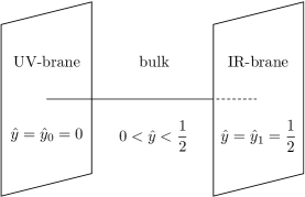
Figure 1: $S^{1}/Z_{2}$ orbifold

4.1 Equivalence classes on the UV-brane

We will prove that, on the UV-brane, any local ECs gauge transformation has the following three unique properties:
(i) the commutative type ($T^{a_{++}}$) generates the identity transformation,
(ii) the mixed type ($T^{a_{+-}}$ or $T^{a_{-+}}$) generates the trivial one that makes $[p,q,r,s]$ invariant,
(iii) the anti-commutative type ($T^{a_{--}}$) generates the trivial or constitutes the following ECs:

$$\begin{split}[p,q,r,s]&\sim[p-1,q+1,r+1,s-1]\quad\text{for $p,s\geq 0$,}\\ &\sim[p+1,q-1,r-1,s+1]\quad\text{for $q,r\geq 0$.}\end{split}$$ (30)

These equivalence relations have been found in Refs. [29, 30]. Thus the consequence in this section is that there are no unknown ECs gauge transformations on the UV-brane.

Le us transform Hermitian $U(N)$ diagonal matrices $P_{i}$ $(i=0,1)$ into other diagonal matrices $P^{\prime}_{i}$ by generators $\{T^{a_{\pm}}\}$ with arbitrary local parameters $f^{a_{\pm}}(\hat{y})$. We again note that $f^{a_{\pm}}(\hat{y})$ are not necessarily invariant to the $S^{1}/Z_{2}$ transformation (2). In the commutative case, the BCs are transformed as

$$\begin{split}P^{\prime}_{i}&=\exp{\left[-i\left\{f^{a_{+}}(\hat{y}_{i}+\hat{y})-f^{a_{+}}(\hat{y}_{i}-\hat{y})\right\}T^{a_{+}}\right]}P_{i}\\ &\to P_{i}\quad(\hat{y}\to 0),\end{split}$$ (31)

where two fixed points are denoted by, $\hat{y}_{0}=0$ $(y_{0}=0)$ and $\hat{y}_{1}=1/2$ $(y_{1}=\pi R)$. Since the parameter functions $f^{a_{+}}(\hat{y})$ are continuous at $\hat{y}=\hat{y}_{0},\,\hat{y}_{1}$, the commutative type generates the identity transformation. This is the same result as the global case (18).

On the other hand, by the anti-commutative generators, we get

$$\begin{split}P^{\prime}_{i}&=\exp{\left[-i\left\{f^{a_{-}}(\hat{y}_{i}+\hat{y})+f^{a_{-}}(\hat{y_{i}}-\hat{y})\right\}T^{a_{-}}\right]}P_{i}\\ &\to e^{-ic^{a_{-}}_{i}T^{a_{-}}}P_{i}\quad(\hat{y}\to 0),\end{split}$$ (32)

where we denote the values of parameters at the fixed points as, $f^{a_{-}}(\hat{y}_{0})=c^{a_{-}}_{0}/2$ and $f^{a_{-}}(\hat{y}_{1})=c^{a_{-}}_{1}/2$. With (31) and (32), we notice that the mixed type makes the BCs $[p,q,r,s]$ invariant as the global case. However, the anti-commutative type rotates $(P_{0},P_{1})$ not simultaneously but independently with $(c^{a_{-}}_{0},c^{a_{-}}_{1})$. It is different from the global case and the ECs (30) are constructed.

As an example, we independently rotate the BCs $[p,q=0,r=0,s]$. For $P_{0}$ and $P_{1}$, the transformation matrices are written as

$$D_{0}\equiv\text{diag}(e^{iT^{--}_{0}})=\begin{pmatrix}\tilde{I}_{p,X}&0\\ 0&\tilde{I}_{s,X}\end{pmatrix},$$ (33)

$$D_{1}\equiv\text{diag}(e^{iT^{--}_{1}})=\begin{pmatrix}\tilde{I}_{p,Y}&0\\ 0&\tilde{I}_{s,Y}\end{pmatrix},$$ (34)

where $X$ and $Y$ satisfy, $0\leq X,Y\leq\min{(p,s)}$ and generally have different values. We count the number of the same and different eigenvalues between $D_{0}$ and $D_{1}$. Let $t$, $u$, and $v$ be respectively the number of the same $+1$, the same $-1$, and the different eigenvalues ($t+u+v=p+s$, $2u+v=2X+2Y$). Then we confirm that the transformations construct

$$[p,q,r,s]\sim[p-v,q+v,r+v,s-v].$$ (35)

This means the equivalence relations (30). We can check that any set of BCs only constitutes the same ECs on the UV-brane.

The properties (i), (ii) and (iii) of the BCs on the UV-brane are caused by the continuity of the transformation parameters $f^{a}(\hat{y})$. For this reason, the local transformations on the UV-brane have the identical behavior with the global ones, except for the anti-commutative type.

4.2 Equivalence classes on the Bulk and IR-brane

As confirmed in Sec. 4.1, on the UV-brane, the commutative type becomes the identity transformation. In contrast, on the bulk or IR-brane, we can show that there exist non-trivial commutative ECs gauge transformations.

We suppose that all of the parameters $\{f^{a_{++}}(\hat{y})\}$ are proportional to a function $f(\hat{y})$, i.e., $f^{a_{++}}(\hat{y})=c^{a_{++}}f(\hat{y})$. The BCs are transformed as

$$P^{\prime}_{i}=\exp{\left[-i\left\{f(\hat{y}_{i}+\hat{y})-f(\hat{y}_{i}-\hat{y})\right\}T^{++}\right]}P_{i}\quad\text{for $0<\hat{y}\leq\frac{1}{2}$ ; $i=0,1$},$$ (36)

where, $T^{++}\equiv c^{a_{++}}T^{a_{++}}$ is a Hermitian $U(N)$ matrix with the commutative form of (13). If $P^{\prime}_{i}$ is different from $P_{i}$ and satisfies the ECs gauge condition (11), the value of $\{f(\hat{y}_{i}+\hat{y})-f(\hat{y_{i}}-\hat{y})\}$ must be a non-zero constant. Such a function does not exist on the UV-brane, but it does on the bulk and IR-brane. In order to show that, we consider the following local parameters with a kink near $\hat{y}=\hat{y}_{0}$ and $\hat{y}=\hat{y}_{1}$ (Fig. 2):

$$f_{0}(\hat{y}) =\frac{1}{2}\tanh{\left[\lambda\left(\hat{y}-(\hat{y}_{0}-\epsilon\right)\right]},$$ (37)

$$f_{1}(\hat{y}) =\frac{1}{2}\tanh{\left[\lambda\left(\hat{y}-(\hat{y}_{1}+\epsilon\right)\right]}.$$ (38)

A small parameter $\epsilon$ is introduced to shift the positions of the kink slightly outward from the fundamental region, $0\leq y\leq\pi R$. Then the gauge fields in the fundamental region are well-defined under the transformations with (37) and (38). We adjust the parameter $\lambda$ to a large value and redefine the area of the bulk as, $1/\lambda\ll\epsilon<\hat{y}<1/2$.

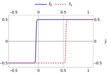
Figure 2: Parameter functions with a kink near the fixed points ($\hat{y}_{0}=0$, $\hat{y}_{1}=0.5$)

On the bulk and IR-brane, (37) and (38) satisfy

$$f_{0}(\hat{y}_{0}+\hat{y})-f_{0}(\hat{y}_{0}-\hat{y})=1,\quad f_{0}(\hat{y}_{1}+\hat{y})-f_{0}(\hat{y}_{1}-\hat{y})=0,$$ (39)

$$f_{1}(\hat{y}_{0}+\hat{y})-f_{1}(\hat{y}_{0}-\hat{y})=0,\quad f_{1}(\hat{y}_{1}+\hat{y})-f_{1}(\hat{y}_{1}-\hat{y})=1.$$ (40)

The phase factors in the transformation matrices are denoted as, $f_{i}^{a_{++}}(\hat{y})T_{i}^{a_{++}}=c_{i}^{a_{++}}f_{i}(\hat{y})T^{a_{++}}=f_{i}(\hat{y})T_{i}^{++}$ ($i=0,1$). Using the generators $T_{0}^{++}$ and $T_{1}^{++}$, the BCs are transformed into $(P^{\prime}_{0},P^{\prime}_{1})=(e^{-iT_{0}^{++}}\!P_{0},\,P_{1})$ and $(P_{0},\,e^{-iT_{1}^{++}}\!P_{1})$, respectively. Therefore, all that remains is to find a set of parameters such that the commutative exponential factor $e^{iT^{++}}$ becomes a non-trivial real diagonal matrix.

Now let us take all sub-matrices in $T^{++}$ diagonal: $T^{++}=diag(a_{1},a_{2},\ldots,a_{N})$. The exponential factor is written as

$$e^{iT^{++}}=\begin{pmatrix}e^{ia_{1}}&&0\\ &\ddots&\\ 0&&e^{ia_{N}}\end{pmatrix}.$$ (41)

The parameters are constrained to, $a_{i}=n_{i}\pi$ $(i=1,2,\ldots,N\,;n_{i}\in\mathbb{Z})$ because of the ECs gauge condition (11). Eventually, through the commutative ECs gauge transformation with the kink parameter $f_{0}$ or $f_{1}$, a Hermitian $U(N)$ matrix $P$ is transformed into

$$P^{\prime}=\tilde{I}P,$$ (42)

where $\tilde{I}$ is a diagonal matrix with components $+1$ or $-1$. By using (37) ((38)), the sign of the components of $P_{0}$ ($P_{1}$) can be freely flipped while $P_{1}$ ($P_{0}$) remains fixed. As a result, all of the diagonal BCs $[p,q,r,s]$ are connected by the commutative ECs gauge transformations on the bulk and IR-brane.

Finally, we mention the anti-commutative transformations on the bulk and IR-brane. In order to satisfy the ECs gauge conditions (11) for the anti-commutative transformations, the parameters $f^{a}(\hat{y})$ must be odd-functions at the two fixed points. These transformations conserve the BCs $[p,q,r,s]$ or constitute the well-known ECs (30), but not new ones.

5 Conclusions and discussions

The arbitrariness problem of the boundary conditions (BCs) has been addressed by comprehensively investigating the existence of the BCs-changing gauge transformations in $SU(N)$ gauge theory on the $S^{1}/Z_{2}$ orbifold. It has been shown that any global transformation makes the diagonal BCs invariant. For the local transformations, we have found that the non-trivial equivalence classes (ECs) on the UV-brane are only the previously well-known ones: $[p,q,r,s]\sim[p\pm 1,q\mp 1,r\mp 1,s\pm 1]$. On the bulk and IR-brane, however, it has been derived that all sets of the diagonal BCs are connected by the commutative local transformations with a kink parameter.

Previous studies implicitly assumed that only the above ECs exist. This assumption is valid only on the UV-brane. On the bulk and IR-brane, the local transformations connect all sets of the BCs. This allows, for instance, the fields on the bulk and IR-brane to retain the original symmetry, since we can select the BCs to the unit matrices. It could lead to modifications to the existing models on the $S^{1}/Z_{2}$ orbifold.

It might also solve the arbitrariness problem of BCs. The number of the ECs was shown in Ref.[26] to be $(N+1)^{2}$. The ECs are still present on the UV-brane. The different ECs were considered to be unconnected, but they are connected in the bulk. This connection might bring a relationship to the ECs on the UV-brane. We expect that some mechanism determines the physically realized ECs, for example, by evaluating the global minimum of the effective potential, as described in Ref.[26]

A new problem emerges through this study, i.e., how should we define the physical observable on the bulk and IR-brane? Due to Hosotani mechanism, the combination of BCs and dynamical Wilson line phases has verified that there is one physics in one ECs. But this statement is valid only when the BCs-changing gauge transformations are anti-commute with the BCs. The commutative gauge transformations break the structure of the Wilson line phase. It means that a physical observable is realized only on the UV-brane. We will continue our work and hope to report on this problem.

References

- [1] N.S. Manton. A new six-dimensional approach to the weinberg-salam model. Nuclear Physics B, 158(1):141–153, 1979.
- [2] D.B. Fairlie. Higgs fields and the determination of the weinberg angle. Physics Letters B, 82(1):97–100, 1979.
- [3] D B Fairlie. Two consistent calculations of the weinberg angle. Journal of Physics G: Nuclear Physics, 5(4):L55, apr 1979.
- [4] Yoshiharu Kawamura. Gauge Symmetry Reduction from the Extra Space S1/Z2. Progress of Theoretical Physics, 103(3):613–619, 03 2000.
- [5] Yoshiharu Kawamura. Triplet-Doublet Splitting, Proton Stability and an Extra Dimension. Progress of Theoretical Physics, 105(6):999–1006, 06 2001.
- [6] Lawrence Hall and Yasunori Nomura. Gauge unification in higher dimensions. Phys. Rev. D, 64:055003, Aug 2001.
- [7] MASAHIRO KUBO, C. S. LIM, and HIROYUKI YAMASHITA. The hosotani mechanism in bulk gauge theories with an orbifold extra space s1/z2. Modern Physics Letters A, 17(34):2249–2263, 2002.
- [8] Claudio A. Scrucca, Marco Serone, and Luca Silvestrini. Electroweak symmetry breaking and fermion masses from extra dimensions. Nuclear Physics B, 669(1):128–158, 2003.
- [9] Csaba Csáki, Christophe Grojean, Hitoshi Murayama, Luigi Pilo, and John Terning. Gauge theories on an interval: Unitarity without a higgs boson. Phys. Rev. D, 69:055006, Mar 2004.
- [10] Gustavo Burdman and Yasunori Nomura. Unification of higgs and gauge fields in five dimensions. Nuclear Physics B, 656(1):3–22, 2003.
- [11] Naoyuki Haba, Yutaka Hosotani, Yoshiharu Kawamura, and Toshifumi Yamashita. Dynamical symmetry breaking in gauge-higgs unification on an orbifold. Phys. Rev. D, 70:015010, Jul 2004.
- [12] Csaba Csáki, Christophe Grojean, and Hitoshi Murayama. Standard model higgs boson from higher dimensional gauge fields. Phys. Rev. D, 67:085012, Apr 2003.
- [13] Kaustubh Agashe, Roberto Contino, and Alex Pomarol. The minimal composite higgs model. Nuclear Physics B, 719(1):165–187, 2005.
- [14] Y. Hosotani, K. Oda, T. Ohnuma, and Y. Sakamura. Dynamical electroweak symmetry breaking in gauge-higgs unification with top and bottom quarks. Phys. Rev. D, 78:096002, Nov 2008.
- [15] Y. Hosotani, K. Oda, T Ohnuma, and Y. Sakamura. Erratum: Dynamical electroweak symmetry breaking in gauge-higgs unification with top and bottom quarks [phys. rev. d 78, 096002 (2008)]. Phys. Rev. D, 79:079902, Apr 2009.
- [16] Shuichiro Funatsu, Hisaki Hatanaka, Yutaka Hosotani, Yuta Orikasa, and Takuya Shimotani. Dark matter in the SO(5) U(1) gauge-Higgs unification. Progress of Theoretical and Experimental Physics, 2014(11), 11 2014. 113B01.
- [17] Shuichiro Funatsu, Hisaki Hatanaka, Yutaka Hosotani, Yuta Orikasa, and Naoki Yamatsu. Electroweak and left-right phase transitions in gauge-higgs unification. Phys. Rev. D, 104:115018, Dec 2021.
- [18] Yutaka Hosotani, Shusaku Noda, and Kazunori Takenaga. Dynamical gauge-higgs unification in the electroweak theory. Physics Letters B, 607(3):276–285, 2005.
- [19] Giuliano Panico, Marco Serone, and Andrea Wulzer. A model of electroweak symmetry breaking from a fifth dimension. Nuclear Physics B, 739(1):186–207, 2006.
- [20] Giuliano Panico, Marco Serone, and Andrea Wulzer. Electroweak symmetry breaking and precision tests with a fifth dimension. Nuclear Physics B, 762(1):189–211, 2007.
- [21] Nobuhito Maru and Yoshiki Yatagai. Fermion mass hierarchy in grand gauge-Higgs unification. Progress of Theoretical and Experimental Physics, 2019(8), 08 2019. 083B03.
- [22] Yuki Adachi and Nobuhito Maru. Revisiting electroweak symmetry breaking and the higgs boson mass in gauge-higgs unification. Phys. Rev. D, 98:015022, Jul 2018.
- [23] Nobuhito Maru, Haruki Takahashi, and Yoshiki Yatagai. Gauge coupling unification in simplified grand gauge-higgs unification. Phys. Rev. D, 106:055033, Sep 2022.
- [24] M Harada, Y Kikukawa, and K Yamawaki. Strong Coupling Gauge Theories and Effective Field Theories. WORLD SCIENTIFIC, 2003.
- [25] M. Quiros. New ideas in symmetry breaking. In Theoretical Advanced Study Institute in Elementary Particle Physics (TASI 2002): Particle Physics and Cosmology: The Quest for Physics Beyond the Standard Model(s), pages 549–601, 2 2003.
- [26] Naoyuki Haba, Yutaka Hosotani, and Yoshiharu Kawamura. Classification and Dynamics of Equivalence Classes in SU(N) Gauge Theory on the Orbifold S1/Z2. Progress of Theoretical Physics, 111(2):265–289, 02 2004.
- [27] Yutaka Hosotani. Dynamical mass generation by compact extra dimensions. Physics Letters B, 126(5):309–313, 1983.
- [28] Yutaka Hosotani. Dynamical gauge symmetry breaking as the casimir effect. Physics Letters B, 129(3):193–197, 1983.
- [29] Yutaka Hosotani. Dynamics of non-integrable phases and gauge symmetry breaking. Annals of Physics, 190(2):233–253, 1989.
- [30] Naoyuki Haba, Masatomi Harada, Yutaka Hosotani, and Yoshiharu Kawamura. Dynamical rearrangement of gauge symmetry on the orbifold s1/z2. Nuclear Physics B, 657:169–213, 2003.
- [31] Yutaka Hosotani, Shusaku Noda, and Kazunori Takenaga. Dynamical gauge symmetry breaking and mass generation on the orbifold . Phys. Rev. D, 69:125014, Jun 2004.
- [32] Yoshiharu Kawamura, Teppei Kinami, and Takashi Miura. Equivalence Classes of Boundary Conditions in Gauge Theory on Z3 Orbifold. Progress of Theoretical Physics, 120(5):815–831, 11 2008.
- [33] Yoshiharu Kawamura and Takashi Miura. Equivalence Classes of Boundary Conditions in SU(N) Gauge Theory on 2-Dimensional Orbifolds. Progress of Theoretical Physics, 122(4):847–864, 10 2009.
- [34] Yoshiharu Kawamura and Yasunari Nishikawa. On diagonal representatives in boundary condition matrices on orbifolds. International Journal of Modern Physics A, 35(31):2050206, 2020.
- [35] Yoshiharu Kawamura, Eiji Kodaira, Kentaro Kojima, and Toshifumi Yamashita. On representation matrices of boundary conditions in gauge theories compactified on two-dimensional orbifolds. 11 2022.