Direct numerical simulation of a zero-pressure-gradient thermal turbulent boundary layer up to $Pr=6$

Abstract

The objective of the present study is to provide a numerical database of thermal boundary layers and to contribute to the understanding of the dynamics of passive scalars at different Prandtl numbers. In this regard, a direct numerical simulation (DNS) of an incompressible zero-pressure-gradient turbulent boundary layer is performed with the Reynolds number based on momentum thickness $Re_{\theta}$ up to $1080$. Four passive scalars, characterized by the Prandtl numbers $Pr=1,2,4,6$ are simulated with constant Dirichlet boundary conditions, using the pseudo-spectral code SIMSON (Chevalier et al., 2007). To the best of our knowledge, the present direct numerical simulation provides the thermal boundary layer with the highest Prandtl number available in the literature. It corresponds to that of water at $\sim$24${}^{o}C$, when the fluid temperature is considered as a passive scalar. Turbulence statistics for the flow and thermal fields are computed and compared with available numerical simulations at similar Reynolds numbers. The mean flow and temperature profiles, root-mean squared (RMS) velocity and temperature fluctuations, turbulent heat flux, turbulent Prandtl number and higher-order statistics agree well with the numerical data reported in the literature. Furthermore, the pre-multiplied two-dimensional spectra of the velocity and of the passive scalars are computed, providing a quantitative description of the energy distribution at the different lengthscales for various wall-normal locations. The energy distribution of the heat flux fields at the wall is concentrated on longer temporal structures and exhibits different footprint at the wall, with increasing Prandtl number.

1 Introduction

Wall-bounded turbulence is a phenomenon of huge technological importance in many industrial and environmental applications. The study of turbulent flow in complex geometries is quite challenging both from the numerical and experimental points of view, but it is relevant for various practical applications. For this reason, simpler geometries are chosen when the fundamental physics of the flow is studied. One canonical flow case widely used in the literature is the boundary layer developing on a flat surface (Schlatter et al., 2009; Sillero et al., 2014). The spatially-evolving fully-turbulent boundary layer has been studied using different experimental techniques (Österlund, 1999; Rahgozar et al., 2013; Shehzad et al., 2021) with the researchers constantly improving the measurement techniques (Örlü & Alfredsson, 2010; Bailey et al., 2013; Vinuesa & Nagib, 2016) to obtain reliable measurements at high Reynolds number (Samie et al., 2018). At the same time, direct numerical investigations of turbulent boundary layer have been performed in several studies (Spalart, 1988; Ferrante & Elghobashi, 2005; Wu & Moin, 2009; Simens et al., 2009; Schlatter et al., 2010) implementing different solution methods for an increasing range of Reynolds number. Since the experimental techniques have resolution limitations in the near-wall region of boundary-layer flow, direct numerical simulations (DNSs) have been helpful to study the relevant transport phenomena (Araya & Castillo, 2012). On the other hand, DNSs are limited to low-Reynolds-number flows owing to high computational cost. The direct numerical simulation of turbulent boundary layer is not only limited to canonical flows but also extended to more complex geometries like airfoils (Vinuesa et al., 2017).

Many engineering applications involve heat and mass transfer, turbulent mixing, combustion, etc. (Kozuka et al., 2009). For this reason, scalar quantities like temperature also become important to be simulated. Understanding and predicting the dynamics of passive scalars like air and water pollutants play an important role in local and global environmental problems (Kasagi & Iida, 1999; Lazpita et al., 2022), as well as in the design of transport and energy systems (Straub et al., 2019).

Several experimental studies (Kays, 1972; Perry & Hoffmann, 1976; Simonich & Bradshaw, 1978; Subramanian & Antonia, 1981; Krishnamoorthy & Antonia, 1987) have analyzed different aspects of heat transfer of passive scalars in turbulent boundary layers. The investigation by Kays (1972) presented the variation of skin-friction coefficient and Stanton number in boundary layer over a transpiring wall, with different blowing and suction conditions for constant free-stream velocity condition. They have also discussed and proposed theoretical models to enable the prediction of heat transfer in a turbulent boundary layer. A zero-pressure gradient turbulent boundary layer with constant wall-temperature conditions was setup by Perry & Hoffmann (1976), which enabled them to test similarity relations between instantaneous heat and momentum fluxes. Simonich & Bradshaw (1978) investigated the effects of the free-stream on heat transfer in a turbulent boundary layer and reported the increase in Stanton number with respect to free-stream turbulence. Subramanian & Antonia (1981) studied the effects of Reynolds number in a turbulent boundary layer and reported the constants in the logarithmic law for velocity and temperature to be independent of Reynolds number. Further, Krishnamoorthy & Antonia (1987) were able to measure the three components of average temperature dissipation very close to the wall in a turbulent boundary layer, in the effort to model turbulence for the temperature fields computation. This is only a small summary of the recent investigations on this topic, as there have been a continual investigation of the heat transfer behaviour both from engineering and numerical-modelling aspects.

In numerical investigations, the fluid temperature can be considered as a passive scalar, provided that the buoyancy effects and the temperature dependence of fluid properties are considered as negligible (Araya & Castillo, 2012). Many DNS studies of turbulent scalar transport have been performed to analyze the convective heat transfer between the fluid and solid walls in spatially-developing flows.  Bell & Ferziger (1993) first performed the DNS for a turbulent thermal boundary layer. Later, Kong et al. (2000) performed a DNS at a Prandtl number of $Pr=0.71$ with different boundary conditions including isothermal (Dirichlet) and isoflux (Neumann), for $Re_{\theta}$ ranging between 300 and 420 (note that $Re_{\theta}$ is the Reynolds number based on momentum thickness). The Reynolds-number range was extended in the studies by Hattori et al. (2007), who simulated $Re_{\theta}$ from $1000$ to $1200$, at $Pr=0.71$. At the same time, the numerical investigations for Prandtl numbers up to $Pr=2$ were performed by Tohdoh et al. (2008) for a relatively lower Reynolds-number range, up to $Re_{\theta}=420$. The effect of different boundary conditions at $Pr=0.2,\,0.71$ and $2.0$ in the Reynolds-number range of $Re_{\theta}\in\left[350,830\right]$ was reported by Li et al. (2009). Differently from thermal channel-flow simulations, which have been conducted at higher Prandtl numbers of 49 and low $Re$ by Schwertfirm & Manhart (2007) and at a $Pr$ of 10 and high Reynolds number by Alcántara-Ávila & Hoyas (2021), the thermal turbulent boundary layers have been only partially explored at a medium Prandtl number of 2 by Li et al. (2009) owing to the significant computational cost associated with higher $Pr$. In this study, we consider higher Prandtl numbers in a turbulent thermal boundary layer, reporting analysis that are currently not available in the literature, according to the authors’ knowledge. Thereby, the passive scalars at $Pr=1,2,4$ and $6$ are simulated for $Re_{\theta}$ up to 1070 in a zero-pressure gradient turbulent boundary layer using an isothermal wall boundary condition.

The details of the simulation setup are provided in $\S$2. The statistics obtained from the simulation at different Prandtl numbers are compared with the data available in the literature for the fully-developed thermal turbulent boundary layer. Since the thermal channel flow and thermal boundary layer exhibit a similar behaviour in the near-wall region, the statistical quantities of the channel flow reported in the literature are compared with the thermal boundary layer quantities at similar Reynolds number. Both comparisons are presented in $\S$3. In $\S$4 we analyze the distribution of energy in different scales for the wall-heat flux field and wall-parallel fields at $y^{+}=15,30$ and $50$ (where the superscript ‘+’ denotes scaling in terms of friction velocity $u_{\tau}$, see below). The premultiplied two-dimensional power-spectral density provide additional insight into the scalar transport at different Prandtl numbers. Finally, a short summary of the observations discussed in this work is reported in $\S$5.

2 Methodology

2.1 Governing equations

A DNS of the zero-pressure-gradient (ZPG) turbulent boundary layer (TBL) is performed using the pseudo-spectral code SIMSON (Chevalier et al., 2007). The code solves the governing equations in non-dimensional form (here, written in index notation), in particular the flow and scalar variables are non-dimensionalized as

$$\tilde{{x}_{i}}=\frac{x_{i}}{\delta_{0}^{*}}\,,\;\tilde{{U}_{i}}=\frac{U_{i}}{U_{\infty}}\,,\;\tilde{t}=\frac{tU_{\infty}}{\delta_{0}^{*}}\,,\;\tilde{P}=\frac{P}{\rho U_{\infty}^{2}}\,,\;\tilde{{\theta}_{i}}=\frac{\theta_{i}-\theta_{i,\infty}}{\theta_{i,w}-\theta_{i,\infty}}\,,$$ (1)

where $\left(x_{1},x_{2},x_{3}\right)=\left(x,y,z\right)$ are the Cartesian coordinates in the streamwise, wall-normal and spanwise directions, respectively and $t$ denotes the time. The length scale used for the non-dimensionalization is the displacement thickness at $x=0$ and $t=0$, denoted by $\delta_{0}^{*}$. The corresponding instantaneous velocity components are denoted by $\left(U_{1},U_{2},U_{3}\right)=\left(U,V,W\right)$ with the mean quantities identified by $\left(\left<U\right>,\left<V\right>,\left<W\right>\right)$ and the fluctuations by $\left(u,v,w\right)$. Here $U_{\infty}$ is the undisturbed laminar free-stream velocity at $x=0$ and time $t=0$. The total pressure is denoted by $P$ and the density and kinematic viscosity of the fluid is represented by $\rho$ and $\nu$, respectively. In this study, four different passive scalars $\left(\theta_{1},\theta_{2},\theta_{3},\theta_{4}\right)$ are simulated at different Prandtl numbers $\left(Pr=1,2,4,6\right)$, respectively. Here, $\theta_{i,\infty},\theta_{i,w}$ correspond to the $i^{th}$ scalar concentration in the free-stream and at the wall, respectively with the mean quantities indicated by $\left<\theta_{i}\right>$ and the corresponding fluctuations by $\theta_{i}^{\prime}$. The superscript $\tilde{\cdot}$ introduced in equation 1 identifies a non-dimensional variable and it shall be dropped in the non-dimensional quantities for the rest of the sections for simplicity.

The non-dimensional form of the incompressible Navier–Stokes equation and the transport equation for passive scalars are given by

$$\frac{\partial U_{i}}{\partial x_{i}} =0\,,$$ (2)

$$\frac{\partial U_{i}}{\partial t}+U_{j}\frac{\partial U_{i}}{\partial x_{j}} =-\frac{\partial P}{\partial x_{i}}+\frac{1}{Re_{\delta_{0}^{*}}}\frac{\partial^{2}U_{i}}{\partial x_{j}\partial x_{j}}+F_{i}\,,$$ (3)

$$\frac{\partial\theta_{i}}{\partial t}+U_{j}\frac{\partial\theta_{i}}{\partial x_{j}} =\frac{1}{Re_{\delta_{0}^{*}}Pr}\frac{\partial^{2}\theta_{i}}{\partial x_{j}\partial x_{j}}+F_{\theta_{i}}\,,$$ (4)

where $Re_{\delta_{0}^{*}}$ identifies the Reynolds number based on the free-stream velocity $\left(U_{\infty}\right)$ and the displacement thickness at the inlet $\left(\delta_{0}^{*}\right)$. The product of Reynolds number $\left(Re_{\delta_{0}^{*}}\right)$ and Prandtl number $\left(Pr\right)$ results in another non-dimensional number called Péclet number ($Pe=Re_{\delta_{0}^{*}}Pr$), which measures the ratio between the scalar convective transport and the scalar molecular diffusion. Here, $F_{i}$ and $F_{\theta_{i}}$ correspond to the volume force terms for the velocity and passive scalars, respectively. The velocity-vorticity formulation of the incompressible Navier–Stokes equation is implemented in the solver as the divergence-free condition is implicitly satisfied by the formulation.

2.2 Boundary conditions

Having defined the governing equations, the problem definition is completed by providing appropriate boundary conditions. At the wall, the velocity of the fluid is the same as that of the solid surface and is given by the following no-slip and no-penetration boundary conditions

$$U\rvert_{y=0}=0\,,\;V\rvert_{y=0}=0\,,\;W\rvert_{y=0}=0\,.$$ (5)

From the continuity equation, we also obtain

$$\left.\frac{\partial V}{\partial y}\right\rvert_{y=0}=0\,.$$ (6)

The flow is assumed to extend to an infinite distance perpendicular to the plate, but discretizing an infinite domain is not feasible. Hence, a finite domain has to be considered, for which artificial boundary conditions have to be applied. A simple Dirichlet condition can be considered; however, the desired flow solution generally contains a disturbance that would be forced to zero. This would introduce an error due to the increased damping of the disturbances in the boundary layer (Lundbladh et al., 1999). An improvement to the aforementioned boundary condition can be made by using the Neumann boundary condition given by

$$\left.\frac{\partial U_{i}}{\partial y}\right\rvert_{y=y_{L}}=\left.\frac{\partial\mathcal{U}_{i}}{\partial y}\right\rvert_{y=y_{L}}\,.$$ (7)

where $y_{L}$ is the height of the solution domain in the wall-normal direction in physical space and $\mathcal{U}_{i}$ is the laminar base flow that is chosen as the Blasius flow for the present study. For the passive scalars an isothermal wall boundary condition is applied, as given by

$$\theta_{i}\rvert_{y=0}=0\,,$$ (8)

which corresponds to a vanishing thermal-activity ratio $K$. The thermal-activity ratio defines the ratio between the fluid density, thermal conductivity and specific heat capacity and the same properties of the boundary surface as defined below

$$K=\sqrt{\frac{\rho kC_{p}}{\rho_{w}k_{w}C_{p,w}}}\,.$$ (9)

Here, $\rho_{w}$, $k_{w}$ and $C_{p,w}$ correspond to the density, thermal conductivity and specific heat capacity of the wall. The isothermal wall boundary condition corresponds to the fluid that exchanges heat with the boundary surface, without modifying the wall temperature. The boundary condition in the free-stream is given by

$$\theta_{i}\rvert_{y=y_{L}}=1\,.$$ (10)

2.3 Numerical scheme

The direct numerical simulation is performed with a pseudo-spectral method, where Fourier expansions are used in the streamwise and spanwise directions and Chebyshev polynomials $T_{k}(\xi)$ (on $-1\leq\xi\geq 1$) are used in the wall-normal direction employing the Chebyshev-tau method for faster convergence rates. The time advancement is performed using the second-order Crank–Nicholson scheme for linear terms and the third-order Runge–Kutta method for non-linear terms with a constant time step $\Delta t$. The non-linear terms are calculated in physical space and the aliasing errors in the evaluation of non-linear terms are removed by the 3/2 rule.

Since the TBL is developing in $x$, the periodic boundary condition cannot be directly used in this particular direction, which requires specific numerical treatment. In this regard, one approach is to impose an appropriate instantaneous velocity and scalar profile at the inlet for every time step. Assuming self-similarity of the flow in the streamwise direction, Lund et al. (1998) proposed a rescaling-recycling method to generate the required inlet profiles based on the solution downstream. An alternative approach is the addition of the fringe region downstream of the physical domain to retain the periodicity in the streamwise direction as described by (Bertolotti et al., 1992; Nordström et al., 1999). In this method, the disturbances are damped, and the flow is forced from the outflow of the physical domain to the same profile as the inflow. The fringe technique is used in the present study, as the inflow conditions from a laminar profile at followed by the tripping produce natural instantaneous fluctuations for the velocity and the scalar fields (Araya & Castillo, 2012). The fringe region is implemented by adding a volume force $\left(F_{i};F_{\theta_{i}}\right)$ to the momentum and scalar transport equation $\left(\ref{nd_momentum},\ref{nd_scalar}\right)$, respectively. The forcing term is given by

$$F_{i}=\lambda(x)\left(\mathcal{U}_{i}-U_{i}\right)\,,$$ (11)

$$F_{\theta_{i}}=\lambda(x)\left(\breve{\theta}_{i}-\theta_{i}\right)\,,$$ (12)

where $\lambda(x)$ is the strength of the forcing which is non-zero only in the fringe region. The flow field at the inlet is the laminar Blasius profile $\mathcal{U}_{i}$ and for the scalar $\theta_{i}$ it is the linear variation with $y$ ranging from 0 to 1, denoted by $\breve{\theta}_{i}$.

2.4 Computational domain and numerical setup

The laminar base flow is tripped by a random volume force strip $\left(\text{at }x/\delta_{0}^{*}=10\right)$ to trigger transition of the flow to a turbulent state. For this simulation, a three-dimensional cuboid is considered with length, height and width equal to $x_{L},y_{L},z_{L}$, respectively. The lower surface of the cuboid is considered as a flat plate with no-slip boundary conditions. The boundary layer grows in the considered computational domain with initial thickness denoted by $\delta_{0}^{*}$. In the streamwise direction, the computational domain terminates the fringe region. The vertical extent of the computational domain includes the whole boundary layer and the domain height is chosen based on the free-stream boundary condition. In particular, the problem setup in this work is similar to that studied by Li et al. (2009).

The computational domain is discretized by $N_{x},N_{y}$ and $N_{z}$ grid points in the streamwise, wall-normal and spanwise directions, respectively. The grid spacing is uniform in the streamwise and spanwise directions. For the wall-normal direction, the collocation points follow the Gauss–Lobatto (GL) distribution given by

$$y_{i}=\cos\left(\pi\frac{i}{N_{y}}\right)\quad i=0,1,2...,N_{y}\,.$$ (13)

The computational box has a dimension of 1000$\,\delta_{0}^{*}\,\times\,$40$\,\delta_{0}^{*}\,\times\,$50$\,\delta_{0}^{*}$ in the streamwise, wall-normal and spanwise directions, respectively. The number of grid points in each direction corresponds to 3200$\,\times\,$385$\,\times\,$320. Considering the friction velocity $u_{\tau}$ at the middle of the computational domain $\left(x/\delta_{0}^{*}=500\text{, corresponding to }Re_{\theta}=794\right)$, the grid resolution in viscous units is $\Delta x^{+}=6.6$ and $\Delta z^{+}=3.3$ in the wall-parallel directions. In the wall-normal direction we have an irregular distribution of collocation points, hence $\Delta y^{+}$ varies between $0.01$ and $3.5$.Note that the smallest scale in the scalar fluctuation is inversely proportional to $Pr^{1/2}$ (Tennekes & Lumley, 1972) and hence, the Batchelor length scale $\eta_{\theta_{i}}$ (which is analogous to the smallest scale in turbulent flow, Kolmogorov scale $\eta$) is estimated as $\eta Pr^{-1/2}$ (Kozuka et al., 2009). Similarly, the ratio of largest to the smallest scales is proportional to $~{}Re^{1.5}Pr^{0.5}$ at high $Pr$ (Batchelor, 1959; Tennekes & Lumley, 1972). In this study, an adequate grid resolution is adopted to resolve all the physically-relevant scales. The Reynolds number based on free-stream velocity and displacement thickness at the inlet is $Re_{\delta_{0}^{*}}=450$ and the friction Reynolds number based on local friction velocity $\left(u_{\tau}\right)$ and boundary-layer thickness $\left(\delta_{99}\right)$ is $Re_{\tau}=46$. At outlet, the Reynolds number based on displacement thickness is $Re_{\delta_{0}^{*}}=1,580$ and $Re_{\tau}=396$.

In this study, five different realizations of ZPG TBL are performed by introducing different trip forcings through modification of the random seed parameter, to obtain an ensemble average of the statistical quantities. All the different realizations are run for about 2,400 time units $\left({\delta_{0}^{*}}/{U_{\infty}}\right)$ after one flow-through of initial transience, which corresponds to 1,000 time units $\left({\delta_{0}^{*}}/{U_{\infty}}\right)$. The converged statistics are obtained with the data corresponding to 12,000 time units $\left({\delta_{0}^{*}}/{U_{\infty}}\right)$.

3 Comparison with data in the literature

3.1 Mean velocity and scalar profiles

The mean velocity profile obtained at the streamwise location corresponding to $Re_{\theta}=670$ is shown in figure 1. The streamwise velocity profile is compared with the DNS data from Spalart (1988) at $Re_{\theta}=670$ and Komminaho & Skote (2002) at $Re_{\theta}=666$. The comparison of the present data with the existing DNS results shows a good agreement in the inner region. There is a slight deviation of the mean velocity profile reported by Spalart (1988) in the wake region with respect to the present data but it agrees well with the data provided by Komminaho & Skote (2002).

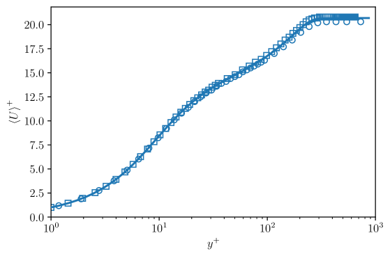
Figure 1: Inner-scaled mean streamwise velocity profile at $Re_{\theta}=670$.  Present DNS,  Spalart (1988),  Komminaho & Skote (2002) at $Re_{\theta}=666$.

The mean profiles of the various passive scalars $\theta_{i}$ at different Prandtl numbers are normalized with the respective Prandtl numbers and with the friction scalar $\theta_{i,\tau}$ defined as

$$\theta_{i,\tau}=\frac{q_{i,w}}{\rho C_{p}u_{\tau}}\,,$$ (14)

where $C_{p}$ is the heat capacity of the fluid and $q_{i,w}$ is the rate of heat transfer from the wall to the fluid and is defined by

$$q_{i,w}=\left.-k\frac{{\rm d}\left<\theta_{i}\right>}{{\rm d}y}\right\rvert_{y=0}\,.$$ (15)

where $k$ is the thermal conductivity of the fluid. The normalized mean scalar profiles are plotted at $Re_{\theta}=1070$, corresponding to $Re_{\tau}=395$, as shown in figure 2. The mean scalar profiles follow the conductive sub-layer relation ($\theta_{i}^{+}=Pry^{+}$) and is clearly identified in the plots for $y^{+}<5$. The profiles of the passive scalars at $Pr=1,2$ are compared against the channel DNS data provided by Kozuka et al. (2009) at the same Prandtl numbers. The comparison shows a good agreement in the near-wall and overlap regions. It should be noted that the boundary condition used by Kozuka et al. (2009) is the uniform heat flux condition as opposed to the uniform temperature boundary condition applied in this study. Note that the study by Kawamura et al. (2000) concluded that the mean scalar profile should be different between the Dirichlet and Neumann boundary conditions based on low-Reynolds-number simulations and associated the difference with the differing scalar von Kármán coefficient $k_{\theta_{i}}$ as given in

$$\frac{\left<\theta_{i}\right>-\left<\theta_{i,w}\right>}{\theta_{i,\tau}}=\frac{1}{k_{\theta_{i}}}\rm{log}\;y^{+}+B_{\theta_{i}}\left(Pr\right)\,,$$ (16)

with $B_{\theta_{i}}$ denoting the additive constant for the scalar $\theta_{i}$. However, based on higher-Reynolds-number simulations, Pirozzoli et al. (2016) reported that the difference in boundary condition affects the mean passive scalar profiles only in small magnitudes in the overlap layer although the effect is evident in the scalar fluctuation profiles reported later.

The scalar profile at $Pr=4$ is compared against the channel DNS data reported by Alcántara-Ávila et al. (2018). The channel DNS data reported by Kozuka et al. (2009) at $Pr=7$ is used for comparison of the passive scalar at $Pr=6$, since there are no simulations reported in the literature at exactly the same Prandtl number. This gives us the opportunity to highlight the difference between the profiles at these high Prandtl numbers. Due to the difference in the considered Prandtl numbers, we observe a discrepancy in the mean velocity profile for $y^{+}>40$ in the overlap region. Since the channel data is used for the comparison, there is a difference observed near the wake region for all the cases. However, a good agreement of the profiles is observed for the inner region. Based on experimental data, semi-empirical fits were provided by Kader (1981) for a boundary layer with constant heat flux. In this study it was assumed that the overlap layer exhibited logarithmic variation as given in equation (16), and an empirical relation was provided to determine the additive constant $B_{\theta_{i}}$. The comparison of the mean scalar profiles against the relationships provided by Kader (1981) shows that the value at the wake is slightly overestimated with respect to the DNS data. The deviation for scalar $\theta_{4}$ corresponding to $Pr=6$ is about 3% for $y^{+}\in\left[100,500\right]$. One possible reason for this small deviation could also be the constant-temperature boundary condition imposed in our simulations as opposed to the constant-heat-flux boundary conditions considered by Kader (1981).

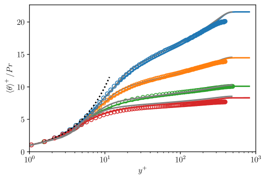
Figure 2: Normalized mean profiles of the passive scalars at $Re_{\theta}=1070$ corresponding to $Re_{\tau}=395$.  $Pr=1$,  $Pr=2$,  $Pr=4$,  $Pr=6$, channel DNS data by Kozuka et al. (2009) at $Re_{\tau}=395$ and  $Pr=1$,  $Pr=2$,  $Pr=7$,  channel DNS data by Alcántara-Ávila et al. (2018) at $Re_{\tau}=500$ and $Pr=4$, with  conductive sub-layer relation, $\theta_{i}^{+}=Pry^{+}$ and  fit by Kader (1981).

3.2 Velocity and scalar fluctuations

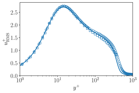
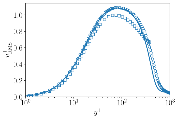
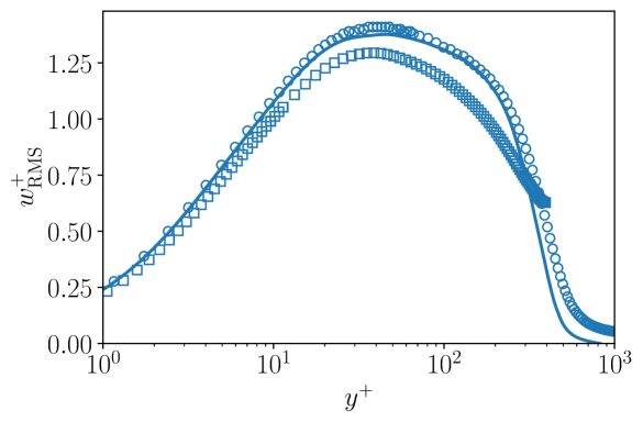
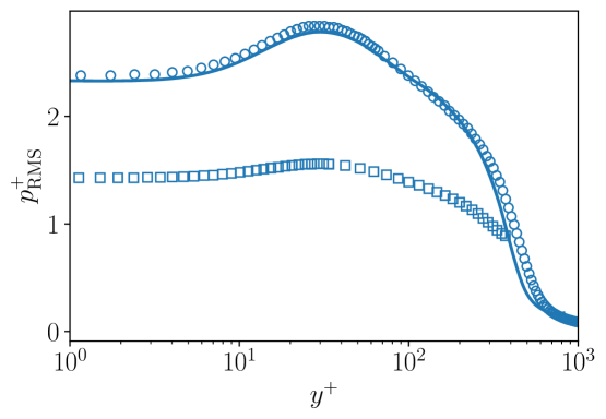
Figure 3: RMS velocity fluctuations and RMS pressure fluctuation at $Re_{\theta}=1070$.  Present DNS,  Jiménez et al. (2010) at $Re_{\theta}=1100$,  channel DNS data of Abe et al. (2004) at $Re_{\tau}=395$.

As shown in figure 3, the present velocity-fluctuation root-mean-squared (RMS) data shows a trend similar to that of the results by Jiménez et al. (2010). The RMS profiles of the three velocity components are in good agreement in the inner region, while a minor difference can be observed in the outer region. Nonetheless, the peaks of the velocity fluctuations match in both position and magnitude. There is a slight offset in the plots of $p_{\rm RMS}$, which can be attributed to the small difference in the considered $Re_{\theta}$ for comparison. The RMS of the velocity components are also compared with the channel DNS data provided by Abe et al. (2004). The streamwise RMS agrees well with the present DNS results and the near-wall peak value coincides with the present observations. As expected, there is a difference observed in the outer region of flow, since channel and boundary layer flows are fundamentally different farther from the wall. Additionally, the RMS of the pressure fluctuations observed in the boundary layer is different compared with the channel flow. From the present DNS data, the peak of the streamwise velocity fluctuation is found at $y^{+}=14$, corresponding in outer units to $y/\delta_{99}=0.035$.

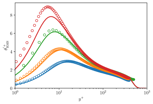
Figure 4: Scalar fluctuation RMS at $Re_{\theta}=1070$. Present DNS data for  $Pr=1$,  $Pr=2$,  $Pr=4$,  $Pr=6$, channel DNS data by Kozuka et al. (2009) at $Re_{\tau}=395$ and  $Pr=1$,  $Pr=2$,  $Pr=7$,  channel DNS data by Alcántara-Ávila et al. (2018) at $Re_{\tau}=500$ and $Pr=4$.

The RMS of the scalars at different Prandtl numbers are plotted in figure 4. The scalar RMS profile at $Pr=1$ is similar to the streamwise velocity RMS and has a higher (roughly 5%) near-wall peak comparatively, as expected. The comparison of scalar-fluctuation profiles at $Pr=1,2$ with the channel DNS data from Kozuka et al. (2009) shows a good agreement in the inner and logarithmic region in addition to a good match of the peak value and wall-normal location. Despite the small difference in $Re_{\tau}$, the profiles at $Pr=4$ as obtained by Alcántara-Ávila et al. (2018) shows a reasonably good agreement with the present results. With increasing Prandtl number, the peak value of the scalar fluctuation RMS increases and is located closer to the wall. The scalar fluctuations decay to zero at the wall due to the isothermal boundary condition and they also decay to zero outside the boundary layer due to the absence of disturbances in the free-stream.

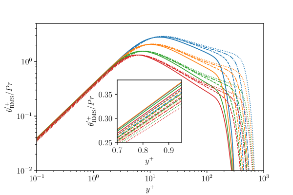
Figure 5: Scalar fluctuations scaled by Prandtl number at  $Pr=1$,  $Pr=2$,  $Pr=4$,  $Pr=6$ and  $Re_{\theta}=420$,  $Re_{\theta}=628$,  $Re_{\theta}=830$,  $Re_{\theta}=1070$ at the corresponding Prandtl numbers.

The obtained scalar-fluctuation RMS profiles are scaled with the respective Prandtl numbers and is plotted in figure 5. We observe that the lines of $\theta^{\prime+}_{\rm RMS}$ for different scalars at different Reynolds numbers are parallel and not coinciding. Similar observations were also made by Alcántara-Ávila et al. (2021) for a particular scalar at $Pr=0.71$ and attributed the differences in the viscous-diffusion term at the wall to the increase in slope of $\theta^{\prime+}_{\rm RMS}$. The slope of $\theta^{\prime+}_{\rm RMS}$ changes with Reynolds number because the peak of $\theta^{\prime+}_{\rm RMS}$ increases and the location of such a peak moves farther from the wall whereas with respect to Prandtl number, the location of $\theta^{\prime+}_{\rm RMS}$ moves closer to the wall as discussed earlier. A correlation for $\theta_{\rm RMS,\,max}^{\prime+}$ was obtained as in Alcántara-Ávila et al. (2021) for each passive scalar considered in the present study as shown in the figure 6. It should be noted that if the maximum value is obtained directly at the collocation point, some variations are observed along $Re_{\tau}$ due to the grid resolution. In order to minimize the high-frequency variation along $Re_{\tau}$ as plotted in figures 6 and 7, a simple convolution operation is performed which does not alter the obtained empirical fits. Clearly, for higher Prandtl numbers of $4,6$, the peak of the scalar-fluctuation RMS tends to decrease with increasing $Re_{\tau}$. When the present DNS data with $Re_{\theta}\in[470,1070]$ and $Pr=1,2,4,6$ is used to find an overall variation of the peak in the scalar-fluctuation RMS we find

$$\theta_{\rm RMS,\,max}^{\prime+}=2.969Re_{\tau}^{-0.00858}Pr^{0.571}\,,$$ (17)

with $R^{2}=0.99$. The observed correlation shows a weak dependence on $Re$ compared with that on $Pr$. Further, from equation (17) a decaying trend of $\theta_{\rm RMS,\,max}^{\prime+}$ with $Re$ is obtained although such a trend has not been observed in the literature except for $\theta_{3},\;\theta_{4}$ in the present study. The studies by Pirozzoli et al. (2016) and Alcántara-Ávila et al. (2021) have reported the increasing trend of $\theta_{\rm RMS,\,max}^{\prime+}$ with respect to $Re$ but for a lower $Pr$ than in the present work. Pirozzoli et al. (2016) have suggested that the attached-eddy arguments support the increase of inner peak of streamwise-velocity RMS with respect to $Re_{\tau}$ due to the effect of overlying attached eddies and they assumed that the same argument applies to the passive scalars. On the other hand, we find that the inner peak of the passive-scalar RMS at high $Pr$ does not follow the previous argumentation. It should also be noted that the range of $Re_{\tau}$ in our present simulation is narrow compared with those of the works by Pirozzoli et al. (2016) and Alcántara-Ávila et al. (2021) and a more detailed investigation of this topic is necessary to make any conclusive statements.

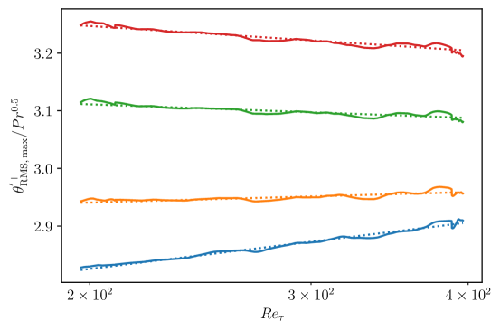
Figure 6: Variation of the peak of scalar fluctuation RMS with respect to $Re_{\tau}$, for  $Pr=1$,  $Pr=2$,  $Pr=4$,  $Pr=6$ including the corresponding empirical fits  $0.116\log{\left(Re_{\tau}\right)}+2.210$ with $R^{2}=0.976$,  $0.037\log{\left(Re_{\tau}\right)}+3.963$ with $R^{2}=0.620$,  $-0.068\log{\left(Re_{\tau}\right)}+6.583$ with $R^{2}=0.726$,  $-0.151\log{\left(Re_{\tau}\right)}+8.753$ with $R^{2}=0.894$.

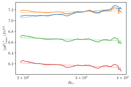
Figure 7: Variation of the peak of streamwise heat flux with respect to $Re_{\tau}$, for  $Pr=1$,  $Pr=2$,  $Pr=4$,  $Pr=6$ including the corresponding empirical fits  $0.250\log{\left(Re_{\tau}\right)}+5.732$ with $R^{2}=0.808$,  $0.064\log{\left(Re_{\tau}\right)}+9.769$ with $R^{2}=0.119$,  $-0.1626\log{\left(Re_{\tau}\right)}+14.223$ with $R^{2}=0.328$,  $-0.293\log{\left(Re_{\tau}\right)}+16.773$ with $R^{2}=0.513$.

The above procedure was also performed for streamwise heat flux as shown in figure 7. A similar behaviour was observed with the overall variation in streamwise heat flux given by

$$\left<u\theta^{\prime}\right>^{+}_{\rm max}=7.74Re_{\tau}^{-0.006}Pr^{0.401}\,,$$ (18)

with $R^{2}=0.9913$.

3.3 Integral quantities and non-dimensional numbers

The shape factor $H_{12}$, which measures the ratio between the displacement thickness $\delta^{*}$ and the momentum thickness $\theta$ is plotted in figure 8. The shape factor is lower in the turbulent region with increasing $Re_{\theta}$ and agrees well with the experimental and numerical data for $Re_{\theta}>600$ where the turbulent boundary layer is fully developed.

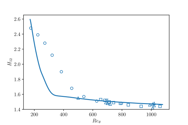
Figure 8: Streamwise evolution of the shape factor $H_{12}$.  Present DNS,  Simens et al. (2009), experimental data by  Roach & Brierly (1990),  Erm & Joubert (1991),  Purtell et al. (1981).

Figure 9 depicts the streamwise variation of the skin-friction coefficient $C_{f}$ for the present simulation and indicates that the obtained result is in good agreement with the turbulent skin-friction solution provided by Schoenherr (1932), which is given by

$$C_{f}=0.31\left[\ln^{2}{\left(2Re_{\theta}\right)}+2\ln{\left(2Re_{\theta}\right)}\right]^{-1}\,.$$ (19)

The computed skin-friction coefficient is also in good agreement with the correlation proposed by Smits et al. (1983), which is given as:

$$C_{f}=0.024Re_{\theta}^{-1/4}\,.$$ (20)

The trip location is at $x/\delta_{0}^{*}=10$ with a strong peak in the skin-friction coefficient followed by the transition to turbulence before $x/\delta_{0}^{*}=200$. The experimental data provided by Erm & Joubert (1991) with wire tripping also closely corresponds to the calculated turbulent skin-friction coefficient. It should be noted that Erm & Joubert (1991) also repeated the experiments with different tripping devices and found the influence of tripping to persist until $Re_{\theta}\approx 1500$. Due to this, Jiménez et al. (2010) found the experimental data to be scattered for $Re_{\theta}<1070$ and also showed the scatter to decrease with $Re_{\theta}>1600$.

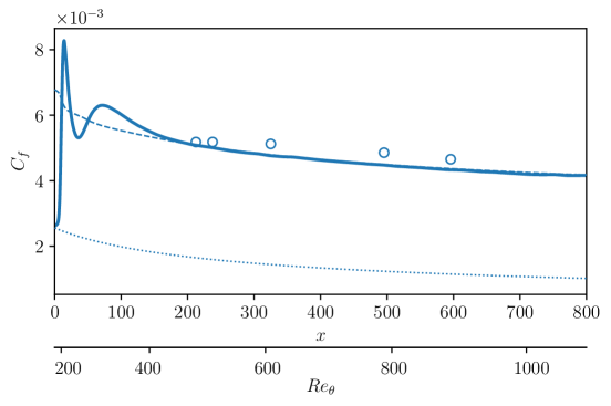
Figure 9: Variation of skin-friction coefficient along the streamwise direction.  Present DNS,  theoretical laminar skin-friction solution,  turbulent solution given by Schoenherr (1932),  experimental data by Erm & Joubert (1991) with wire tripping.

The Stanton number normalizes the convective heat transfer into the fluid with respect to the thermal capacity of the fluid. The spatial evolution of the Stanton numbers for different passive scalars scaled with the square-root of $Pr$ (as plotted in figure 10) is very similar to the skin-friction profiles plotted in figure 9. There is a difference observed in the laminar Stanton-number at $x=0$ with the present scaling. However, the individual Stanton-number profiles are well-corresponding to the laminar solution given by Kays & Crawford (1993) which is

$$St=\frac{0.332}{\sqrt{Re_{x}}Pr^{2/3}}\,,$$ (21)

and with the turbulent solution obtained from the Reynolds–Colburn analogy as given by Lienhard & John (2005). For $\theta_{1}$, due to Reynolds analogy the Stanton profile matches with the skin-friction profile scaled by a factor of two. For the passive scalars at higher Prandtl numbers, a generalization of the Reynolds–Colburn analogy can be obtained, as reported in the study by Lienhard (2020):

$$St=\frac{Nu}{Re_{x}Pr}=\frac{C_{f}/2}{a_{1}+a_{2}\left(Pr^{a_{3}}-1\right)\sqrt{C_{f}/2}}\,,$$ (22)

with the values of $a_{1}=1,a_{2}=12.8$ and $a_{3}=0.68$ provided in Lienhard & John (2005) and $C_{f}$ being expressed as

$$C_{f}=\frac{0.455}{\ln^{2}{\left(0.06Re_{x}\right)}}\,.$$ (23)

The Stanton-number plot for the passive scalar at $Pr=6$ agrees well with the turbulent solution obtained from the Reynolds–Colburn analogy as shown in figure 10. On the other hand, reference curves for Kays and Crawford and the Reynolds–Colburn analogy are only reported for $\theta_{4}$ for clarity.

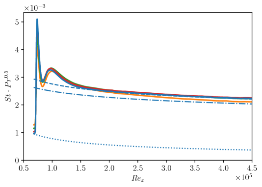
Figure 10: Variation of Stanton number along the streamwise direction for different passive scalars.  $\theta_{1}\,$,  $\theta_{2}$,  $\theta_{3}$,  $\theta_{4}$,  Kays & Crawford (1993) correlation corresponding to $\theta_{4}$ and  Reynolds–Colburn analogy as given by Lienhard & John (2005) plotted for $\theta_{4}$,  interpolation developed by Hollingsworth Jr. (1989) plotted for $\theta_{4}$.

Using the data for water with $Pr=5.9$, Hollingsworth Jr. (1989) developed an interpolation for Prandtl numbers from 0.7 to 5.9 assuming the critical thickness of the sub-layer to be a simple function of Prandtl number. The empirical expression is given by

$$St=0.02426Pr^{-0.895}Re_{x}^{-0.1879Pr^{-0.18}}\,,$$ (24)

which is plotted for the scalar at $Pr=6$ in figure 10. We find that the relationship proposed by Hollingsworth Jr. (1989) under predicts the Stanton number at $Pr=6$. However, the interpolation relation provides a good match with the calculated Stanton number for $\theta_{1}$, better than the Reynolds–Colburn analogy, which is not indicated in the plot for clarity.

Using the data obtained in the present simulation, a correlation between the Nusselt, Prandtl and Reynolds numbers can be obtained as:

$$Nu_{x}=0.02Re_{x}^{0.828}Pr^{0.514}\,,$$ (25)

which yields $R^{2}=0.9985$. This is similar to the correlation proposed by Kays & Crawford (1980) but for fully-developed profiles in circular tubes and computed for gases:

$$Nu=0.021Re^{0.8}Pr^{0.5}\,.$$ (26)

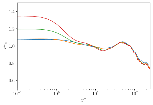
Figure 11: Variation of turbulent Prandtl number with respect to wall-normal distance in inner scale at $Re_{\theta}=1070$ for passive scalar at  $Pr=1$,  $Pr=2$,  $Pr=4$,  $Pr=6$.

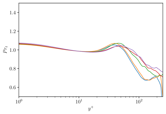
Figure 12: Variation of turbulent Prandtl number with respect to wall-normal distance in inner scale at  $Re_{\theta}=396$,  $Re_{\theta}=420$,  $Re_{\theta}=628$,  $Re_{\theta}=830$,  $Re_{\theta}=1070$ for a passive scalar at $Pr=1$.

An important parameter for scalar transport is the turbulent Prandtl number $Pr_{t}$, which is defined as the ratio between turbulent eddy viscosity and turbulent eddy diffusivity:

$$Pr_{t}=\frac{\nu_{t}}{\alpha_{t}}\,.$$ (27)

The eddy viscosity and the eddy diffusivity arise from the Boussinesq hypothesis Boussinesq (1877) for modelling turbulent stresses and the heat-flux vector, respectively. For parallel flows (the ones in which the velocity profile does not vary in the streamwise direction), the turbulent eddy viscosity and the turbulent eddy diffusivity are used to describe the turbulent momentum transfer and heat transfer with respect to the mean-flow conditions, in particular the mean velocity strain and temperature gradients, respectively. They are defined as:

$$\nu_{t}=-\frac{\left<u^{\prime}v^{\prime}\right>}{{\partial\left<u\right>}/{\partial y}}$$ (28)

and

$$\alpha_{t}=-\frac{\left<v^{\prime}\theta^{\prime}\right>}{{\partial\left<\theta\right>}/{\partial y}}\,.$$ (29)

It should be noted that the eddy viscosity or diffusivity does not represent a physical property of the fluid, like the molecular viscosity, rather a property of the flow. The Reynolds analogy introduces the similarity between the turbulent momentum exchange and turbulent heat transfer in a fluid. Reynolds (1874) noted that, for a fully-turbulent field, both the momentum and heat are transferred due to the motion of turbulent eddies. This yields a simpler model for the turbulent Prandtl number, where the turbulent eddy viscosity for the momentum exchange and turbulent eddy diffusivity for the scalar transport are equal, such that $Pr_{t}=1$.

Substitution of the eddy viscosity and diffusivity into the definition of turbulent Prandtl number results in

$$Pr_{t}=\frac{\left<u^{\prime}v^{\prime}\right>}{\left<v^{\prime}\theta^{\prime}\right>}\frac{{\partial\left<\theta\right>}/{\partial y}}{{\partial\left<u\right>}/{\partial y}}\,.$$ (30)

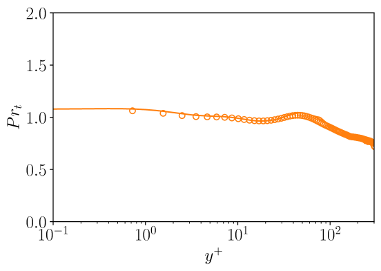
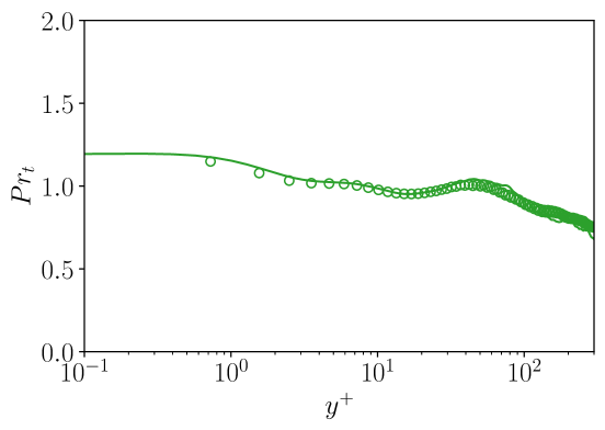
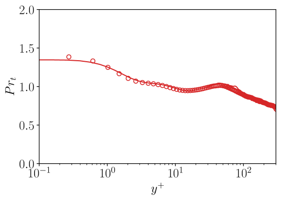
Figure 13: Comparison of turbulent Prandtl number against the channel DNS data at $Re_{\theta}=1070$ for different molecular Prandtl numbers. Present DNS for  $Pr=1$,  $Pr=2$,  $Pr=4$,  $Pr=6$, channel DNS data by Alcántara-Ávila & Hoyas (2021) at $Re_{\tau}=497$ and  $Pr=1$,  $Pr=2$,  $Pr=4$,  $Pr=6$.

From this definition, evaluating the turbulent Prandtl number at any point in the boundary layer would require the turbulent shear stress, turbulent heat transfer, velocity gradient and temperature gradient. Experimental investigations have limited accuracy in the simultaneous measurement of the Reynolds shear stress and wall-normal turbulent heat flux, in particular close to the wall (Araya & Castillo, 2012). For this reason, experimental investigations like Blom (1970), Antonia (1980), Kays & Crawford (1993) exhibit significant scatter in the data.

The variation of turbulent Prandtl number with the wall-normal distance in inner units at a given $Re_{\theta}=1070$ is reported in figure 11. We observe that the turbulent Prandtl number varies at the wall and increases with respect to molecular Prandtl number of the scalar. From figure 12, we also see the turbulent Prandtl number decays for $y^{+}>15$ and this decay becomes steeper as $Re$ decreases. The turbulent Prandtl number is usually assumed to be a constant and is independent of molecular Prandtl number and wall-normal distance (Li, 2007). Studies such as the ones by Kestin & Richardson (1963) and Blom (1970) have analyzed experimentally the turbulent Prandtl number in order to assess the validity of this assumption. Such experimental investigations have reported a constant value of turbulent Prandtl number as the wall is approached, see figure 11. However, different experimental campaigns provided data that could not show a conclusive interpretation of the behaviour of turbulent Prandtl number close to the wall.

For the different passive scalars considered in the present study, the turbulent Prandtl number approaches a constant value $>1$ close to the wall in the viscous sub-layer. The plots of $Pr_{t}$ exhibit a significant difference closer to the wall with respect to the various molecular Prandtl numbers. There is a slight decrease in $Pr_{t}$ up to $y^{+}\approx 20$ and then the increase is maintained farther from the wall up to $y^{+}\approx 50$, the point after which the trend steadily decreases. It is pointed out in Kays (1994) that the peak between $y^{+}\approx 20$ and $100$ is not observed in the experimental data, an observation which was attributed to the high Reynolds number of the experiments, while DNS data is not available for comparison. Our data is consistent with these experimental observations.

Following the discussions about a constant $Pr_{t}$ in the logarithmic region, Kays & Crawford (1993) proposed a correlation for turbulent Prandtl number that is applicable to air. In this correlation, the value of $Pr_{t}$ approaches a constant value of 0.85 in the logarithmic region. In the studies by Hollingsworth Jr. (1989), a correlation was proposed based on the measurement of the temperature profile of water at $Pr\approx 6$. Again, the value of $Pr_{t}$ approaches a value of 0.85 as $y^{+}$ is increased. This observation of constant $Pr_{t}$ in the logarithmic region is not clearly observed with the present DNS data. This can be due to the low-Reynolds number range considered in the present study. Based on the correlation proposed by Hollingsworth Jr. (1989), Kays (1994) suggested a constant value of $Pr_{t}=1.07$ for $0<y^{+}<5$. Indeed, if we consider only the passive scalars at $Pr=1,2$, the turbulent Prandtl number approaches a constant value of 1.07 closer to the wall. It appears that the turbulent Prandtl number is independent of the molecular Prandtl number as shown in the studies by Li et al. (2009). This independence of the turbulent Prandtl number at the wall with respect to the molecular Prandtl number has also been reported in many other studies like Kong et al. (2000) and Jacobs & Durbin (2000) for TBL flow, as well as in Kim & Moin (1989) and Kasagi et al. (1992) for turbulent channel flow. However, from the present study, we find that the turbulent Prandtl number indeed depends on the molecular Prandtl number and this observation is based on the increasing value of $Pr_{t}$ at the wall with respect to the scalars with $Pr=4,6$ as shown in figure 11.

In order to verify the plausibility of the present observations at $Pr=4,6$, the obtained DNS data was compared with the DNS channel data reported by Alcántara-Ávila & Hoyas (2021). Figure 13 shows the comparison of $Pr_{t}$ at different molecular Prandtl numbers where the present DNS data was at $Re_{\theta}=1070$, corresponding to $Re_{\tau}=395$, and the data from Alcántara-Ávila & Hoyas (2021) was at $Re_{\tau}=500$. Despite these differences, the turbulent Prandtl numbers close to the wall are in good agreement, confirming that the $Pr$-scaled wall-normal heat flux decreases with increase in $Pr$ for $Pr\gtrapprox 4$, as stated by Alcántara-Ávila & Hoyas (2021). Thus, the present observation confirms the constant behaviour of the turbulent Prandtl number very close to the wall and highlights its dependence on the molecular Prandtl number, which has been often ignored in turbulent heat-transfer calculations.

A brief discussion of the Reynolds stress budget is provided in Appendix A.

3.4 Higher order statistics, shear stress and heat flux

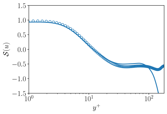
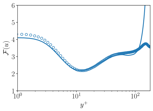
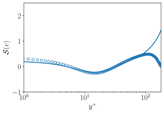
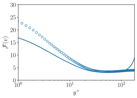
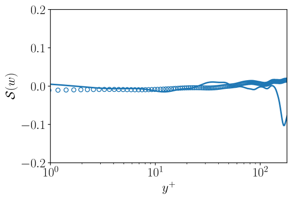
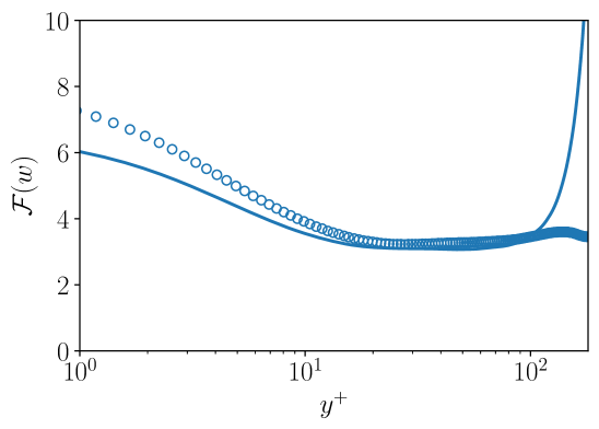
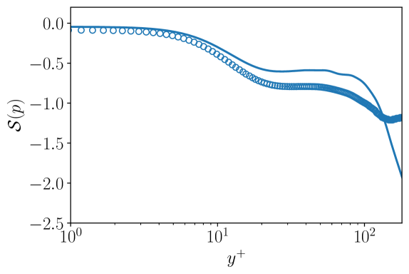
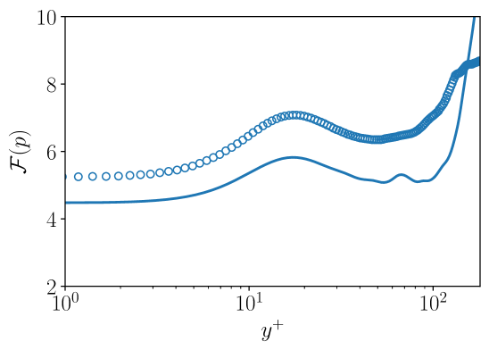
Figure 14: Skewness and flatness for the streamwise, wall-normal and spanwise velocity components at $Re_{\theta}=420$ corresponding to $Re_{\tau}=180$.  Present DNS,  channel DNS data by Vreman & Kuerten (2014) at $Re_{\tau}=180$.

The higher-order statistics (in specific, the values of third and fourth-order moments of a quantity) provides information on the non-Gaussian behaviour of turbulence. The third and fourth-order moments are also called as skewness and flatness, respectively and for a statistically stationary variable $m$, it is defined as

$$\mathcal{S}(m) =\left<m^{3}\right>/\left<m^{2}\right>^{3/2}\,,$$ (31)

$$\mathcal{F}(m) =\left<m^{4}\right>/\left<m^{2}\right>^{2}\,.$$ (32)

If the stochastic variable $m$ were to follow a Gaussian probability distribution, then $\mathcal{S}(m)=0$ and $\mathcal{F}(m)=3$. The deviation from such values for the skewness and flatness of the streamwise and wall-normal velocity components is shown in figure 14 whereas, for the spanwise velocity we observe a Gaussian behaviour in the overlap region as expected. The higher order moments obtained by Vreman & Kuerten (2014) for the turbulent channel flow is compared with the present TBL results at $Re_{\tau}=180$ (corresponding to $Re_{\theta}=420$), showing a reasonable agreement. From figure 9, it should be highlighted that $Re_{\theta}=420$ is roughly in the beginning of the turbulent regime and the deviation of the profiles for $y^{+}>100$ as observed in figure 14 is due to the intermittent wake region which decay to the values for Gaussian distribution as free-stream is approached. There are some differences observed in the overlap region where, the skewness of $u$ is roughly $10\%$ higher than that reported by Vreman & Kuerten (2014). Although the plots indicate an overall good agreement, some drastic differences are observed in the flatness of wall-normal and spanwise velocity components close to the wall, where the turbulence is highly intermittent. The flatness of wall-normal velocity component approaches a value of $\approx 29$ close to the wall for the data provided by Vreman & Kuerten (2014) whereas in the TBL, it converges to $\approx 20$. This is still lower than the value of $22$ obtained by Kim et al. (1987). The skewness of pressure fluctuations is roughly 20% higher in the overlap region of TBL compared to the channel. Further, the intermittency (flatness) of pressure is higher than the velocity components as reported by Kim et al. (1987) whereas the data obtained with TBL shows an offset of 15% throughout and is lower than the flatness behaviour observed in the channel. The flatness factor for pressure fluctuation at the wall approaches a value of 4.5 in the present simulations as compared to the values of 4.7 (Li et al., 2009) and 4.9 (Schewe, 1983), whereas a value of $\approx$5.2 is reported by Vreman & Kuerten (2014).

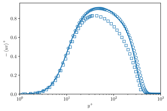
Figure 15: Inner-scaled Reynolds shear stress as a function of the wall-normal direction at $Re_{\theta}=1070$.  Present DNS,  Jiménez et al. (2010) at $Re_{\theta}=1100$,  channel DNS data by Kozuka et al. (2009) at $Re_{\tau}=395$.

The Reynolds shear stress is plotted in figure 15 and it is compared with the turbulent boundary layer data provided by Jiménez et al. (2010) and the channel DNS data by Kozuka et al. (2009). Even if there is a good agreement between the data in the inner region, there is a clear difference in the overlap region between the channel and the turbulent boundary layer. Such differences were also observed in the plots of the fluctuations in the streamwise and wall-normal directions shown in figure 3. The peak of the Reynolds shear stress is higher for the turbulent boundary layer compared to a channel flow, which indicates a higher momentum transfer by the fluctuating velocity field in the turbulent boundary layer. Looking at the energy budgets for shear stress component in both the channel and turbulent boundary layer corresponding to $Re_{\tau}=395$ (plots not shown here), we find that there is higher production in the turbulent boundary layer compared to channel flows (with uniform heat flux wall conditions) in the overlap region whereas the dissipation was of similar magnitude.

The turbulent streamwise heat flux shows a reasonable agreement with the channel data available at $Pr=1,2$, as shown in figure 16 although the peaks for the channel-flow data are slightly higher and closer to the wall compared to the present observations. For $Pr=4$, however, the peak of the streamwise heat flux is higher in the channel data by Alcántara-Ávila et al. (2018), since the heat flux is reported at a higher Reynolds number than our DNS. Furthermore, the comparison at the highest $Pr$ in our simulation was at a slightly lower $Pr$ than that in the channel and hence there is a difference in the slope of the streamwise heat flux close to the wall. Figure 17 shows the wall-normal heat flux for the different simulations. A clear difference can be observed in the outer region when comparing similar Prandtl numbers. On the other hand, the boundary-layer data and the channel data show a better agreement in the inner region.

The correlation coefficients provide more information on the statistical association between the fields, and here the structure of the flow field and scalar fluctuations are analyzed in terms of

$$R_{u\theta} =\frac{\left<u\theta^{\prime}\right>}{u_{\rm{RMS}}\theta^{\prime}_{\rm{RMS}}}\,,$$ (33)

$$R_{v\theta} =\frac{\left<v\theta^{\prime}\right>}{v_{\rm{RMS}}\theta^{\prime}_{\rm{RMS}}}\,.$$

The correlation-coefficient plot in figure 18 corresponding to $u-\theta$ shows a strong correlation of streamwise velocity and scalar fluctuations at $Pr=1$ and it decreases with increase in Prandtl number. This is related to the similarity in the momentum and passive-scalar transport by the turbulent eddies close to the wall. On the other hand, the $v-\theta$ correlation coefficient also shown in figure 18 exhibits an increasing trend with the Prandtl number. In the conductive sub-layer the correlation coefficients coincide for the various Prandtl numbers under study and then approach different values at the wall. This highlights a similar behaviour of the turbulent wall-normal momentum and passive-scalar fields with a caveat, i.e. the differences are present very close to the wall for different Prandtl numbers.

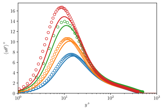
Figure 16: Variation of streamwise heat flux along the wall-normal direction at $Re_{\theta}=1070$ for different passive scalars. Present DNS data for  $Pr=1$,  $Pr=2$,  $Pr=4$,  $Pr=6$, channel DNS data by Kozuka et al. (2009) at $Re_{\tau}=395$ and  $Pr=1$,  $Pr=2$,  $Pr=7$,  channel DNS data by Alcántara-Ávila et al. (2018) at $Re_{\tau}=500$ and $Pr=4$.

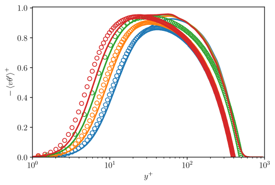
Figure 17: Variation of wall-normal heat flux along the wall-normal direction at $Re_{\theta}=1070$ for different passive scalars. Present DNS data for  $Pr=1$,  $Pr=2$,  $Pr=4$,  $Pr=6$, channel DNS data by Kozuka et al. (2009) at $Re_{\tau}=395$ and  $Pr=1$,  $Pr=2$,  $Pr=7$,  channel DNS data by Alcántara-Ávila et al. (2018) at $Re_{\tau}=500$ and $Pr=4$.

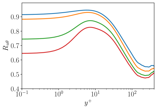
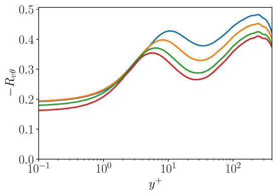
Figure 18: Correlation coefficients: (left) $u-\theta$, (right) $v-\theta$. Present DNS data for scalars at  $Pr=1$,  $Pr=2$,  $Pr=4$,  $Pr=6$ at $Re_{\theta}=1070$.

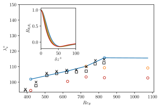
Figure 19: Variation of mean spanwise streak spacing along the streamwise direction at $y^{+}\approx 7$.  $U$,  $\theta_{1}$,  $\theta_{2}$,  $\theta_{3}$,  $\theta_{4}$. Comparison data from Li et al. (2009) for   $U$,  $\theta_{2}$. (Inset) Spanwise two-point correlation for  $\theta_{1}$,  $\theta_{2}$,  $\theta_{3}$,  $\theta_{4}$ at $Re_{\theta}\approx 830$.

3.5 Spanwise two-point correlations

The two-point correlations provide some quantitative information of the turbulent structures near the wall. For example, the streak spacing near the wall is of interest and can also be observed in an experimental setting. In order to identify the mean streak spacing, spanwise two-point correlations of the velocity components and passive scalars were obtained at five different positions along the streamwise direction at different wall-normal positions. Overall, the obtained results at $Re_{\theta}=830$ were compared with the data reported by Kim et al. (1987) and shows good agreement (not shown here). The obtained two-point correlations for different scalars at $Re_{\theta}=830$ are shown in figure 19 to assess the differences for varying $Pr$. The two-point correlation becomes negative and reaches a minimum at an inner-scaled correlation length of $\delta z^{+}\approx 50$. The length at which the minimum occurs provides an estimate of the half-mean separation between the streaks in the spanwise direction, i.e. $\left(\lambda_{s}^{+}/2\right)$. The streak spacing is plotted along the streamwise direction at a wall-normal position of $y^{+}\approx 7$ as shown in figure 19. Overall, the velocity and scalar streak spacing increase with $Re_{\theta}$ as reported in the works of Li et al. (2009) and Schlatter et al. (2009). Note that the correlations are available only at five streamwise locations, but the comparison with Li et al. (2009) is in reasonably good agreement for the velocity and scalar streaks at $Pr=2$. The velocity-streak spacing increases from 102 to 115 and appears to saturate for $Re_{\theta}>830$. Note that such a saturation of streak spacing was also pointed out by Li et al. (2009) for $Re_{\theta}>1500$. From figure 19, we also observe that the streak spacing decreases with increasing $Pr$ and that the streak spacings for the scalars at $Pr=4,6$ are indistinguishable, although the rate of decay of the two-point correlations for the scalars is different. A higher grid resolution might be necessary to quantify the possible differences in the scalar-streak spacing at higher $Pr$.

3.6 Scaling of wall-heat-flux fields

The wall-shear and heat-flux fields at different Prandtl numbers are normalized by subtracting the mean and dividing by the corresponding RMS quantities. The normalization of a quantity $n$ is calculated as:

$$\overline{n}=\frac{n-\left<n\right>}{n_{\rm RMS}}\,.$$ (34)

Figure 20 shows the instantaneous normalized streamwise wall-shear and heat-flux fields at different Prandtl numbers. The normalized fields appear qualitatively similar and this result is confirmed by the distribution of the data in the streamwise shear and heat flux fields obtained from 3,700 samples, shown in figure 21. Though the distribution of data is different in the various fields, after normalization the distributions becomes identical. This indicates the uniformity in the distribution of the fluctuations of shear and heat flux when scaled with the corresponding RMS quantities. This observation is useful for certain applications, for instance in the prediction of fluctuating flow quantities from the wall, as discussed in the study by Guastoni et al. (2022).

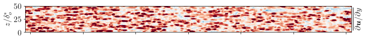
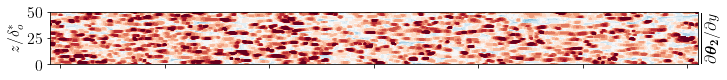
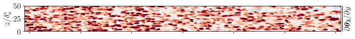
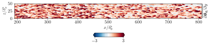
Figure 20: Instantaneous normalized streamwise wall-shear and heat-flux fields at different Prandtl numbers.

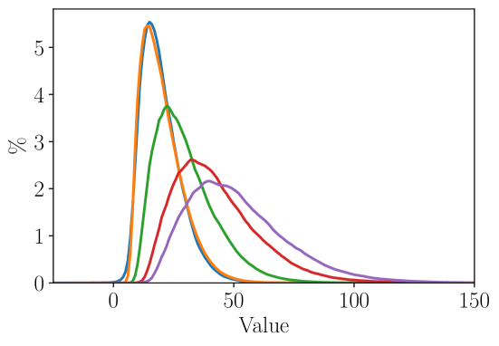
Figure 21: Probability density function of wall-shear and heat-flux fields at different Prandtl numbers. (Left) distribution of absolute data in the fields with a bin size of 1 unit, (right) distribution of the normalized data in the fields with a bin size of 0.1 unit,  ${\partial u}/{\partial y}$ or $\overline{{\partial u}/{\partial y}}$,  ${\partial\theta_{1}}/{\partial y}$ or $\overline{{\partial\theta_{1}}/{\partial y}}$,  ${{\partial\theta_{2}}/{\partial y}}$ or $\overline{{\partial\theta_{2}}/{\partial y}}$,  ${{\partial\theta_{3}}/{\partial y}}$ or $\overline{{\partial\theta_{3}}/{\partial y}}$,  ${{\partial\theta_{4}}/{\partial y}}$ or $\overline{{\partial\theta_{4}}/{\partial y}}$.

4 Spectral analysis

The analysis of thermal-boundary-layer statistics reveals that the scalar fluctuations and heat flux are strongly affected by the Prandtl number of the scalar in the flow and the corresponding scalings were reported in $\S$3. Additional insight can be obtained by analyzing the energy distribution at the different lengthscales for the scalars at the simulated Prandtl numbers. In this regard, time series of the wall-shear, wall-heat flux, streamwise velocity and different scalars were sampled at different wall-normal locations with a sampling time ($\sim$$\Delta t^{+}_{s}=1$ with the reference friction velocity at $x/\delta_{0}^{*}=500$) corresponding to 12,000 time units $\left({\delta_{0}^{*}}/{U_{\infty}}\right)$. The two-dimensional (2D) premultiplied power-spectral density (PSD) $k_{z}k_{t}\phi\left(\lambda_{z}^{+},\lambda_{t}^{+}\right)$ is obtained in the spanwise direction and in time based on the time series, for a total sampled time of about 11.5 flow-through times. Note that here $k$ denotes wavenumber and $\phi$ is the power-spectral density defined for the particular quantity under study.

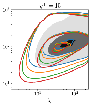
Figure 22: Two-dimensional premultiplied power-spectral density of (left) streamwise wall-shear and wall-heat-flux fields and (right) streamwise velocity and scalar at $y^{+}=15$, for the ZPG thermal TBL with $Re_{\theta}$ ranging from 467 to 1072. The three contour lines correspond to 10%, 50% and 90% of the maximum energy density. We show: $k_{t}k_{z}\phi_{u_{y}u_{y}}$ or $k_{t}k_{z}\phi_{uu}$ (shaded contours),  $k_{t}k_{z}\phi_{{\theta_{1}}_{y}{\theta_{1}}_{y}}$ or $k_{t}k_{z}\phi_{{\theta_{1}}{\theta_{1}}}$,  $k_{t}k_{z}\phi_{{\theta_{2}}_{y}{\theta_{2}}_{y}}$ or $k_{t}k_{z}\phi_{{\theta_{2}}{\theta_{2}}}$,  $k_{t}k_{z}\phi_{{\theta_{3}}_{y}{\theta_{3}}_{y}}$ or $k_{t}k_{z}\phi_{{\theta_{3}}{\theta_{3}}}$,  $k_{t}k_{z}\phi_{{\theta_{4}}_{y}{\theta_{4}}_{y}}$ or $k_{t}k_{z}\phi_{{\theta_{4}}{\theta_{4}}}$, correspondingly. Here, the spatial coordinate in subscript denotes partial derivative with respect to that coordinate.

For the calculation of power-spectral density, the procedure outlined in Pozuelo et al. (2022) is utilized. After the mean subtraction of the sampled time series to obtain the turbulent quantities, first a one-dimensional spectrum $E\left[t,x\right]\left(\lambda_{z}^{+}\right)$ is obtained by performing a fast Fourier transform (FFT) in the spanwise direction, due to the periodicity condition imposed along $z$. As a result, a spectral decomposition of the energy content into different wavenumbers $k_{z}$ is obtained with the corresponding wavelengths $\lambda_{z}$ given by $2\pi/k_{z}$. Note that the local friction velocity is used to obtain the inner-scaled quantities. It should be pointed out that the flow is developing along the streamwise direction and hence the FFT along the streamwise direction is not applicable. In the present spectral analysis, we consider the $Re_{\theta}$ range between 470 and 1070 and use Welch’s overlapping-window method to address the non-periodicity in the temporal signal. As a next step, the spectrum in time is obtained using Welch’s method with 15 bins in total, where 8 of them are independent. A Hamming window is used for imposing the periodicity in the bins, and the 2D spectrum is obtained as $E\left[x\right]\left(\lambda_{z}^{+},\lambda_{t}^{+}\right)$ by using FFT along $z$ and Welch method in $t$. The obtained spectrum is divided by $\Delta k_{t}\Delta k_{z}$ and premultiplied with $k_{t}k_{z}$. Finally, an averaging along $x$ is performed to yield the 2D premultiplied power-spectral density $k_{t}k_{z}\phi\left(\lambda_{z}^{+},\lambda_{t}^{+}\right)$.

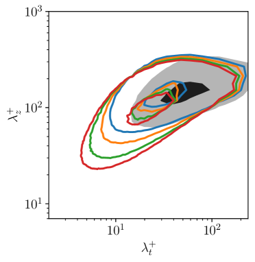
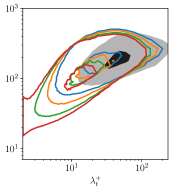
Figure 23: Two-dimensional premultiplied power-spectral density of streamwise velocity and scalar fields at (left) $y^{+}=30$ and (right) $y^{+}=50$. The two contour lines correspond to 10% and 50% of the maximum energy density. We show: $k_{t}k_{z}\phi_{uu}$ (shaded contours),  $k_{t}k_{z}\phi_{{\theta_{1}}{\theta_{1}}}$,  $k_{t}k_{z}\phi_{{\theta_{2}}{\theta_{2}}}$,  $k_{t}k_{z}\phi_{{\theta_{3}}{\theta_{3}}}$,  $k_{t}k_{z}\phi_{{\theta_{4}}{\theta_{4}}}$.

The 2D power-spectral densities of the streamwise wall-shear and wall-heat-flux at different Prandtl numbers are provided in figure 22, along with the power-spectral density of the streamwise velocity and scalar fluctuations at $y^{+}=15$. The obtained 2D power-spectral density at $y^{+}=15$ agrees well with the results reported by Pozuelo et al. (2022), although the latter are at higher Reynolds number. At the wall, the spectral peak is observed at $\lambda_{z}^{+}\approx 100$ and $\lambda_{t}^{+}\approx 100$. Furthermore, at $y^{+}=15$, we observe the maximum of spectral-energy distribution is at $\lambda_{z}^{+}\approx 120$, which corresponds to the characteristic streak spacing in wall turbulence (Smith & Metzler, 1983). It is observed that the power-spectral density for the streamwise wall-shear stress is very similar to that for the wall-heat-flux at $Pr=1$, which is an expected result for the reasons outlined in $\S$9. However, with increasing $Pr$, the power-spectral density shifts to the right, indicating that the energy is not spread over a wider range of scales, and instead is concentrated on longer temporal structures. One could argue that, with a shorter boundary layer, the structures at $Pr=6$ can become larger than the one we develop at $Pr=1$. Because of this, the larger structures have a different footprint at the wall. Additionally, the plots in the figure 22 also exhibit a slight trend downwards for higher $Pr$, a fact that indicates the presence of smaller spanwise scales, in agreement with the discussion in $\S$3.5. Overall, the temporal wavelength range at which we have the most energetic structures in the wall-heat-flux fields increases for larger Prandtl numbers. From the above observations, considering the dominant energetic structures to be composed of streaks at the wall, the scalar at $Pr=6$ (in general for higher $Pr$) might exhibit longer and thinner scalar streak structures at the wall compared with the case at $Pr=1$.

The power-spectral densities calculated at $y^{+}=30$ and $50$ are shown in figure 23. From this figure, we observe that the similarity in the distribution of energy for the scalar at $Pr=1$ and the streamwise velocity is lost as we move farther from the wall. In contrast to the observation of large streamwise structures at the wall, we find an increasing concentration of energy in smaller scales as we increase the Prandtl number. Further, the range of scales in which the energy is distributed also increases with $Pr$. Focusing on the most energetic structures, we find that these are concentrated in a region of smaller temporal and spanwise scales with increasing $Pr$ at both $y^{+}=30$ and $50$. For the scalar at $Pr=6$, the spectral peak is observed at $\lambda_{z}^{+}\approx 100$ and $\lambda_{t}^{+}\approx 20$ for $y^{+}=30$ and $50$.

5 Summary and conclusions

In the present study, a direct numerical simulation of the thermal turbulent boundary layer is performed up to $Re_{\theta}=1080$ with passive scalars at $Pr=1,2,4$ and $6$, which to authors’ knowledge is the highest Prandtl number simulated for the thermal boundary layer. Various statistical quantities for the flow and scalars were computed and compared against the reported channel and TBL data in the literature. Overall, the statistical quantities are in good agreement with the existing data whenever a comparison is possible. For higher $Pr$, we also observed that the peak of the scalar fluctuations decreases when $Re_{\tau}$ increases, which is different from the trend reported in the literature. Further, we showed that the variation of the peak in scalar fluctuation has a weak dependence with $Re_{\tau}$ compared to Prandtl number. Similarly, the peak in the heat flux also exhibits a weak dependence with $Re_{\tau}$ compared to $Pr$ of the scalar and the heat flux scales as ${\sim}Pr^{0.4}$.

In the present study, we also highlighted the behaviour of the turbulent Prandtl number $Pr_{t}$, which does not approach a constant value of 1.07 as the wall is approached for higher Prandtl numbers. In addition, we also found the corresponding $Pr_{t}$ to increase with $Pr$, confirming the findings of Alcántara-Ávila & Hoyas (2021). Finally, a brief description of the energy distribution in the scales for different $Pr$ at different wall-normal locations is presented by analyzing the 2D pre-multiplied power-spectral density.

The analysis and data provided in this work are expected to serve as a database for the research community to assess the validity of new turbulence models and validate other numerical and experimental results.

Appendix A Reynolds stress budget

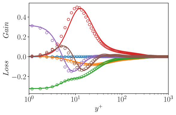
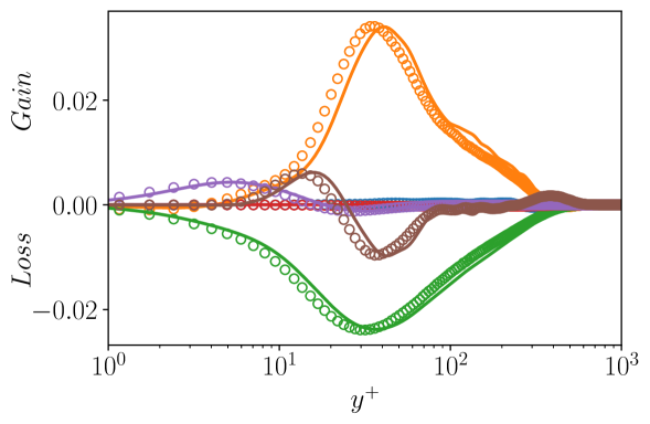
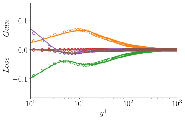
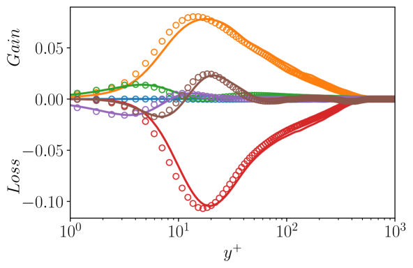
Figure 24: Comparison of the Reynolds-stress budgets. (Top-left) $\left<uu\right>$, (top-right) $\left<vv\right>$, (bottom-left) $\left<ww\right>$, (bottom-right) $\left<uv\right>$,  present DNS,  Jiménez et al. (2010),  convection,  velocity-pressure diffusion,  dissipation,  production,  molecular diffusion,  turbulent diffusion.

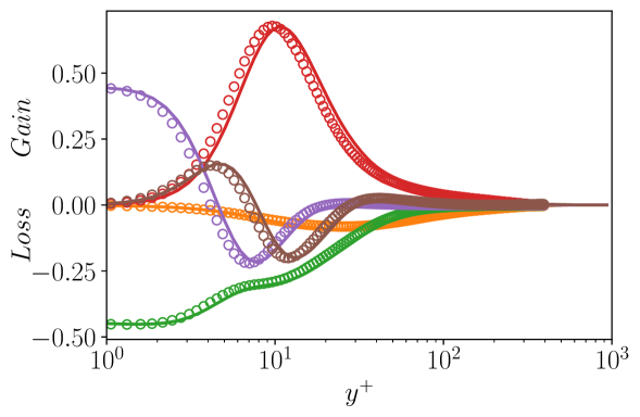
Figure 25: Comparison of the scalar-flux budgets. (Left) $\left<u\theta^{\prime}\right>$, (right) $\left<v\theta^{\prime}\right>$,  present DNS at $Pr=2$,  Kozuka et al. (2009) at $Pr=2$,  convection,  scalar-pressure diffusion,  dissipation,  production,  molecular diffusion,  turbulent diffusion.

Figure 26: Comparison of the scalar-flux budgets. (Left) $\left<u\theta^{\prime}\right>$, (right) $\left<v\theta^{\prime}\right>$,  present DNS at $Pr=6$,  Kozuka et al. (2009) at $Pr=7$,  convection,  scalar-pressure diffusion,  dissipation,  production,  molecular diffusion,  turbulent diffusion.

The Reynolds stress equation is written (in index notation) as:

$$\frac{\bar{D}\left<u_{i}u_{j}\right>}{\bar{D}t}=\mathcal{P}_{ij}-\epsilon_{ij}+C_{ij}+D_{ij}+T_{ij}\,,$$ (35)

where $\bar{D}$ represents the material derivative and $\left<u_{i}u_{j}\right>$ is the Reynolds stress tensor. Here, $\mathcal{P}_{ij}$ denotes the production term, $\epsilon_{ij}$ is the viscous dissipation rate tensor, $C_{ij}$ is the velocity pressure-gradient term (which can be split into pressure strain term and pressure diffusion term), $T_{ij}$ is the turbulent diffusion and $D_{ij}$ is the molecular diffusion term. The corresponding terms are written respectively as:

$$\mathcal{P}_{ij} :=-\left<u_{i}u_{k}\right>\frac{\partial\left<U_{i}\right>}{\partial x_{k}}-\left<u_{j}u_{k}\right>\frac{\partial\left<U_{j}\right>}{\partial x_{k}}\,,$$ (36)

$$\epsilon_{ij} :=2\nu\left<\frac{\partial u_{i}}{\partial x_{k}}\frac{\partial u_{j}}{\partial x_{k}}\right>\,,$$ (37)

$$C_{ij} :=-\frac{1}{\rho}\left<u_{i}\frac{\partial p}{\partial x_{j}}+u_{j}\frac{\partial p}{\partial x_{i}}\right>\,,$$ (38)

$$T_{ij} :=-\frac{\partial}{\partial x_{k}}\left<u_{i}u_{j}u_{k}\right>\,,$$ (39)

$$D_{ij} :=\nu\frac{\partial^{2}}{\partial x_{j}\partial x_{j}}\left<u_{i}u_{j}\right>\,.$$ (40)

Detailed description of the above terms can be found in Pope (2000) and they are non-dimensionalized by $u_{\tau}^{4}/\nu$.

The obtained Reynolds-stress budgets at $Re_{\theta}=1080$ (which is located almost at the end of the computational domain before fringe region) are compared with the data by Jiménez et al. (2010) in the turbulent boundary layer at $Re_{\theta}=1100$ as shown in figure 24. All the different components contributing to the stress terms are in good agreement with the reference data. Due to the lack of TBL data at higher Prandtl numbers, the budgets for the scalar at $Pr=2$ are compared against the channel DNS data from Kozuka et al. (2009) as shown in figure 25. Overall, there is a good comparison obtained for the different terms in the scalar flux budgets. Also as discussed in $\S$3.4, we observe a higher production compared with the channel-flow case for the vertical-heat-flux budget in the overlap region. In addition, the scalar-pressure diffusion term also exhibits the same behaviour as discussed above and it should be noted that the discrepancy not only stems from the different problem setup but also the wall boundary condition for the scalar, which is Dirichlet in the present study and Neumann in the works of Kozuka et al. (2009). Further, a comparison of the data obtained at $Pr=6$ with the data obtained by Kozuka et al. (2009) at $Pr=7$ for a channel flow is also provided in figure 26. Overall, the comparison of the stress budgets at different parameter points shows a good agreement with the data available in the literature. Note that the small discrepancy observed in figure 25 are due to the different Prandtl numbers.

[Acknowledgements]The simulations were run with the computational resources provided by the Swedish National Infrastructure for Computing (SNIC). The authors of the various data bases used in this study are acknowledged for sharing the simulation data. All the data to reproduce the results obtained in the present study will be available on GitHub upon publication.

[Funding]This work is supported by the funding provided by the Swedish e-Science Research Centre (SeRC), ERC grant no. ”2021-CoG-101043998, DEEPCONTROL” to RV and the Knut and Alice Wallenberg (KAW) Foundation.

[Declaration of interests]The authors report no conflict of interest.

References

- Abe et al. (2004) Abe, H., Kawamura, H. & Matsuo, Y. 2004 Surface heat-flux fluctuations in a turbulent channel flow up to with and . Int. J. Heat Fluid Flow 25 (3), 404–419.
- Alcántara-Ávila & Hoyas (2021) Alcántara-Ávila, F. & Hoyas, S. 2021 Direct numerical simulation of thermal channel flow for medium–high Prandtl numbers up to . Int. J. Heat Mass Transf. 176, 121412.
- Alcántara-Ávila et al. (2021) Alcántara-Ávila, F., Hoyas, S. & Pérez-Quiles, M.J. 2021 Direct numerical simulation of thermal channel flow for and . J. Fluid Mech. 916, A29.
- Alcántara-Ávila et al. (2018) Alcántara-Ávila, F., Hoyas, S. & Pérez-Quiles, M. J. 2018 DNS of thermal channel flow up to for medium to low Prandtl numbers. Int. J. Heat Mass Transf. 127, 349–361.
- Antonia (1980) Antonia, R.A. 1980 Behaviour of the turbulent Prandtl number near the wall. Int. J. Heat Mass Transf. 23, 906–908.
- Araya & Castillo (2012) Araya, G. & Castillo, L. 2012 DNS of turbulent thermal boundary layers up to . Int. J. Heat Mass Transf. 55 (15-16), 4003–4019.
- Bailey et al. (2013) Bailey, S.C.C., Hultmark, M., Monty, J.P., Alfredsson, P.H., Chong, M.S., Duncan, R.D., Fransson, J.H.M., Hutchins, N., Marusic, I., McKeon, B.J., Nagib, H.M., Örlü, R., Segalini, A., Smits, A.J. & Vinuesa, R. 2013 Obtaining accurate mean velocity measurements in high Reynolds number turbulent boundary layers using Pitot tubes. J. Fluid Mech. 715, 642–670.
- Batchelor (1959) Batchelor, G.K. 1959 Small-scale variation of convected quantities like temperature in turbulent fluid Part 1. General discussion and the case of small conductivity. J. Fluid Mech. 5 (1), 113–133.
- Bell & Ferziger (1993) Bell, D.M. & Ferziger, J.H. 1993 Turbulent boundary layer DNS with passive scalars. In Near-Wall Turbulent Flows (ed. R. M. C. So, C. G. Speziale, B. E. Launder), pp. 327–336, Elsevier Science.
- Bertolotti et al. (1992) Bertolotti, F.P., Herbert, T. & Spalart, P.R. 1992 Linear and nonlinear stability of the Blasius boundary layer. J. Fluid Mech. 242, 441–474.
- Blom (1970) Blom, J. 1970 An experimental determination of the turbulent Prandtl number in a developing temperature boundary layer. PhD thesis, Technical University of Eindhoven.
- Boussinesq (1877) Boussinesq, J. 1877 Essai sur la théorie des eaux courantes. Mem. Savants Etrangers Acad. Sci. Paris 26, 1–680.
- Chevalier et al. (2007) Chevalier, M., Schlatter, P., Lundbladh, A. & Henningson, D.S. 2007 SIMSON : a pseudo-spectral solver for incompressible boundary layer flows. Tech. Rep. TRITA-MEK 2007:07. KTH Mechanics, Stockholm, Sweden.
- Erm & Joubert (1991) Erm, L.P. & Joubert, P.N. 1991 Low-Reynolds-number turbulent boundary layers. J. Fluid Mech. 230, 1–44.
- Ferrante & Elghobashi (2005) Ferrante, A. & Elghobashi, S. 2005 Reynolds number effect on drag reduction in a microbubble-laden spatially developing turbulent boundary layer. J. Fluid Mech. 543, 93–106.
- Guastoni et al. (2022) Guastoni, L., Balasubramanian, A. G., Güemes, A., Ianiro, A., Discetti, S., Schlatter, P., Azizpour, H. & Vinuesa, R. 2022 Non-intrusive sensing in turbulent boundary layers via deep fully-convolutional neural networks. Preprint, arXiv:2208.06024.
- Hattori et al. (2007) Hattori, H., Houra, T. & Nagano, Y. 2007 Direct numerical simulation of stable and unstable turbulent thermal boundary layers. Int. J. Heat Fluid Flow 28 (6), 1262–1271.
- Hollingsworth Jr. (1989) Hollingsworth Jr., D. K. 1989 Measurement and prediction of the turbulent thermal boundary layer in water on flat and concave surfaces. PhD thesis, Stanford University.
- Jacobs & Durbin (2000) Jacobs, R.G. & Durbin, P.A. 2000 Bypass transition phenomena studies by computer simulation. Tech. Rep. Report no. TF-77. Mech. Eng. Dept., Stanford University.
- Jiménez et al. (2010) Jiménez, J., Hoyas, S., Simens, M.P. & Mizuno, Y. 2010 Turbulent boundary layers and channels at moderate Reynolds numbers. J. Fluid Mech. 657, 335–360.
- Kader (1981) Kader, B.A. 1981 Temperature and concentration profiles in fully turbulent boundary layers. Int. J. Heat Mass Transf. 24 (9), 1541–1544.
- Kasagi & Iida (1999) Kasagi, N. & Iida, O. 1999 Progress in direct numerical simulation of turbulent heat transfer. In Proc. Fifth ASME/JSME Joint Thermal Engg. Conf. (ed. D. L. Dwoyer & M. Y. Hussaini), pp. 15–19, Springer.
- Kasagi et al. (1992) Kasagi, N., Tomita, Y. & Kuroda, A. 1992 Direct numerical simulation of passive scalar field in a turbulent channel flow. J. Heat Transfer 114 (3), 598–606.
- Kawamura et al. (2000) Kawamura, H., Abe, H. & Shingai, K. 2000 DNS of turbulence and heat transport in a channel flow with different Reynolds and Prandtl numbers and boundary conditions. In Proc. Third Int. Symp. on Turbulence, Heat and Mass Transfer (ed. Y. Nagano), pp. 15–32, Engineering Foundation.
- Kays (1972) Kays, W.M. 1972 Heat transfer to the transpired turbulent boundary layer. Int. J. Heat Mass Transf. 15 (5), 1023–1044.
- Kays (1994) Kays, W.M. 1994 Turbulent Prandtl number. Where are we? J. Heat Transfer 116 (2), 284–295.
- Kays & Crawford (1980) Kays, W.M. & Crawford, M.E. 1980 Convective Heat and Mass Transfer McGraw Hill Book Company. New York .
- Kays & Crawford (1993) Kays, W.M. & Crawford, M.E. 1993 Convective Heat and Mass Transfer McGraw-Hill. New York pp. 255–282.
- Kestin & Richardson (1963) Kestin, J. & Richardson, P.D. 1963 Heat transfer across turbulent, incompressible boundary layers. Int. J. Heat Mass Transf. 6 (2), 147–189.
- Kim & Moin (1989) Kim, J. & Moin, P. 1989 Transport of passive scalars in a turbulent channel flow. In Turbulent Shear Flows, Vol. 6 (ed. J.C. Andre et al.), pp. 85–96, Springer.
- Kim et al. (1987) Kim, J., Moin, P. & Moser, R. 1987 Turbulence statistics in fully developed channel flow at low Reynolds number. J. Fluid Mech. 177, 133–166.
- Komminaho & Skote (2002) Komminaho, J. & Skote, M. 2002 Reynolds stress budgets in Couette and boundary layer flows. Flow Turbul. Combust. 68 (2), 167–192.
- Kong et al. (2000) Kong, H., Choi, H. & Lee, J.S. 2000 Direct numerical simulation of turbulent thermal boundary layers. Phys. Fluids 12 (10), 2555–2568.
- Kozuka et al. (2009) Kozuka, M., Seki, Y. & Kawamura, H. 2009 DNS of turbulent heat transfer in a channel flow with a high spatial resolution. Int. J. Heat Fluid Flow 30 (3), 514–524.
- Krishnamoorthy & Antonia (1987) Krishnamoorthy, L.V. & Antonia, R.A. 1987 Temperature-dissipation measurements in a turbulent boundary layer. J. Fluid Mech. 176, 265–281.
- Lazpita et al. (2022) Lazpita, E., Martínez-Sánchez, Á., Corrochano, A., Hoyas, S., Le Clainche, S. & Vinuesa, R. 2022 On the generation and destruction mechanisms of arch vortices in urban fluid flows. Phys. Fluids 34 (5), 051702.
- Li (2007) Li, Q. 2007 Direct numerical simulation of a turbulent boundary layer with passive scalar transport. Tech. Rep. KTH Royal Institute of Technology.
- Li et al. (2009) Li, Q., Schlatter, P., Brandt, L. & Henningson, D.S. 2009 Dns of a spatially developing turbulent boundary layer with passive scalar transport. Int. J. Heat Fluid Flow 30 (5), 916–929.
- Lienhard & John (2005) Lienhard, I.V. & John, H. 2005 A heat transfer textbook. Phlogiston Press.
- Lienhard (2020) Lienhard, J. H. 2020 Heat transfer in flat-plate boundary layers: a correlation for laminar, transitional, and turbulent flow. J. Heat Transfer 142 (6).
- Lund et al. (1998) Lund, T.S., Wu, X. & Squires, K.D. 1998 Generation of turbulent inflow data for spatially-developing boundary layer simulations. J. Comput. Phys. 140 (2), 233–258.
- Lundbladh et al. (1999) Lundbladh, A., Berlin, S., Skote, M., Hildings, C., Choi, J., Kim, J. & Henningson, D.S. 1999 An efficient spectral method for simulation of incompressible flow over a flat plate. Tech. Rep. KTH/MEK/TR–99/11–SE. KTH Mechanics, Stockholm, Sweden.
- Nordström et al. (1999) Nordström, J., Nordin, N. & Henningson, D.S. 1999 The fringe region technique and the Fourier method used in the direct numerical simulation of spatially evolving viscous flows. SIAM J. Sci. Comput. 20 (4), 1365–1393.
- Örlü & Alfredsson (2010) Örlü, R. & Alfredsson, P.H. 2010 On spatial resolution issues related to time-averaged quantities using hot-wire anemometry. Exp. Fluids 49 (1), 101–110.
- Österlund (1999) Österlund, J.M. 1999 Experimental studies of zero pressure-gradient turbulent boundary layer flow. PhD thesis, KTH Royal Institute of Technology.
- Perry & Hoffmann (1976) Perry, A.E. & Hoffmann, P.H. 1976 An experimental study of turbulent convective heat transfer from a flat plate. J. Fluid Mech. 77 (2), 355–368.
- Pirozzoli et al. (2016) Pirozzoli, S., Bernardini, M. & Orlandi, P. 2016 Passive scalars in turbulent channel flow at high Reynolds number. J. Fluid Mech. 788, 614–639.
- Pope (2000) Pope, S.B. 2000 Turbulent flows. Cambridge university press.
- Pozuelo et al. (2022) Pozuelo, R., Li, Q., Schlatter, P. & Vinuesa, R. 2022 An adverse-pressure-gradient turbulent boundary layer with nearly constant up to . J. Fluid Mech. 939.
- Purtell et al. (1981) Purtell, L.P., Klebanoff, P.S. & Buckley, F.T. 1981 Turbulent boundary layer at low Reynolds number. Phys. Fluids 24 (5), 802–811.
- Rahgozar et al. (2013) Rahgozar, S., Maciel, Y. & Schlatter, P. 2013 Spatial resolution analysis of planar PIV measurements to characterise vortices in turbulent flows. J. Turbul. 14 (10), 37–66.
- Reynolds (1874) Reynolds, O. 1874 On the extent and action of the heating surface for steam boilers. Manchester Lit. Phil. Soc. 14, 7–12.
- Roach & Brierly (1990) Roach, P.E. & Brierly, D.H. 1990 The influence of a turbulent free-stream on zero pressure gradient transitional boundary layer development: Part 1. Test cases T3A and T3B. In Numerical Simulation of Unsteady Flows and Transition to Turbulence, pp. 319–347, Cambridge University Press.
- Samie et al. (2018) Samie, M., Marusic, I., Hutchins, N., Fu, M.K., Fan, Y., Hultmark, M. & Smits, A.J. 2018 Fully resolved measurements of turbulent boundary layer flows up to . J. Fluid Mech. 851, 391–415.
- Schewe (1983) Schewe, G. 1983 On the structure and resolution of wall-pressure fluctuations associated with turbulent boundary-layer flow. J. Fluid Mech. 134, 311–328.
- Schlatter et al. (2010) Schlatter, P., Li, Q., Brethouwer, G., Johansson, A.V. & Henningson, D.S. 2010 Simulations of spatially evolving turbulent boundary layers up to . Int. J. Heat Fluid Flow 31 (3), 251–261.
- Schlatter et al. (2009) Schlatter, P., Örlü, R., Li, Q., Brethouwer, G., Fransson, J.H.M., Johansson, A.V., Alfredsson, P.H. & Henningson, D.S. 2009 Turbulent boundary layers up to studied through simulation and experiment. Phys. Fluids 21 (5), 051702.
- Schoenherr (1932) Schoenherr, K.E. 1932 Resistance of flat surfaces moving through a fluid. Trans. Soc. Nav. Archit. Mar. Eng. 40, 279–313.
- Schwertfirm & Manhart (2007) Schwertfirm, F. & Manhart, M. 2007 DNS of passive scalar transport in turbulent channel flow at high Schmidt numbers. Int. J. Heat Fluid Flow 28 (6), 1204–1214.
- Shehzad et al. (2021) Shehzad, M., Sun, B., Jovic, D., Ostovan, Y., Cuvier, C., Foucaut, J.M., Willert, C., Atkinson, C. & Soria, J. 2021 Investigation of large scale motions in zero and adverse pressure gradient turbulent boundary layers using high-spatial-resolution particle image velocimetry. Exp. Therm. Fluid Sci. p. 110469.
- Sillero et al. (2014) Sillero, J.A., Jiménez, J. & Moser, R.D. 2014 Two-point statistics for turbulent boundary layers and channels at Reynolds numbers up to . Phys. Fluids 26 (10), 105109.
- Simens et al. (2009) Simens, M.P., Jiménez, J., Hoyas, S. & Mizuno, Y. 2009 A high-resolution code for turbulent boundary layers. J. Comput. Phys. 228 (11), 4218–4231.
- Simonich & Bradshaw (1978) Simonich, J.C. & Bradshaw, P. 1978 Effect of free-stream turbulence on heat transfer through a turbulent boundary layer. Trans. ASME: J. Heat Transfer 100, 671–677.
- Smith & Metzler (1983) Smith, C.R. & Metzler, S.P. 1983 The characteristics of low-speed streaks in the near-wall region of a turbulent boundary layer. J. Fluid Mech. 129, 27–54.
- Smits et al. (1983) Smits, A.J., Matheson, N. & Joubert, P.N. 1983 Low-Reynolds-number turbulent boundary layers in zero and favorable pressure gradients. J. Ship Res. 27 (03), 147–157.
- Spalart (1988) Spalart, P.R. 1988 Direct simulation of a turbulent boundary layer up to . J. Fluid Mech. 187, 61–98.
- Straub et al. (2019) Straub, S., Forooghi, P., Marocco, L., Wetzel, T., Vinuesa, R., Schlatter, P. & Frohnapfel, B. 2019 The influence of thermal boundary conditions on turbulent forced convection pipe flow at two Prandtl numbers. Int. J. Heat Mass Transf. 144, 118601.
- Subramanian & Antonia (1981) Subramanian, C.S. & Antonia, R.A. 1981 Effect of Reynolds number on a slightly heated turbulent boundary layer. Int. J. Heat Mass Transf. 24 (11), 1833–1846.
- Tennekes & Lumley (1972) Tennekes, H. & Lumley, J.L. 1972 A first course in turbulence. MIT press.
- Tohdoh et al. (2008) Tohdoh, K., Iwamoto, K. & Kawamura, H. 2008 Direct numerical simulation of passive scalar transport in a turbulent boundary layer. In Proceedings of the 7th International ERCOFTAC Symposium on Engineering Turbulence Modelling and Measurements, Limassol, Cyprus, pp. 169–174.
- Vinuesa et al. (2017) Vinuesa, R., Hosseini, S.M., Hanifi, A., Henningson, D.S. & Schlatter, P. 2017 Pressure-gradient turbulent boundary layers developing around a wing section. Flow Turbul. Combust. 99 (3), 613–641.
- Vinuesa & Nagib (2016) Vinuesa, R. & Nagib, H.M. 2016 Enhancing the accuracy of measurement techniques in high Reynolds number turbulent boundary layers for more representative comparison to their canonical representations. Eur. J. Mech. B Fluids 55, 300–312.
- Vreman & Kuerten (2014) Vreman, A.W. & Kuerten, J.G.M. 2014 Comparison of direct numerical simulation databases of turbulent channel flow at . Phys. Fluids 26 (1), 015102.
- Wu & Moin (2009) Wu, X. & Moin, P. 2009 Direct numerical simulation of turbulence in a nominally zero-pressure-gradient flat-plate boundary layer. J. Fluid Mech. 630, 5–41.