A Role of Fractional Dimension in Study Physics

Abstract

We study physics from a fractional dimensional perspective. It is considered that the whole space is not only integer dimensions but also a superposition of spaces between integer dimensions. Space-filling between integer dimensions makes a fractional dimensional space. This happens through a rotation of the integer dimension by the fractional derivative operator (local part) to sweep all spaces between two integer dimensions. Then, we introduce four axioms which they can help us to build a mathematical framework for study physics from fractional dimension point of view. Afterward, three scenarios such as static, linear and quadratic trajectories are demonstrated. Where moving with linear or quadratic trajectories in fractional dimensional space corresponds to an inertial framework or accelerated system in physics, respectively. Also from this opinion, it is realized that the coupling of space and time (space-time) happens through the dimension with an interconnection role where we call it space-dimension-time. Finally, the wave equation is derived from fractional dimensional point of view with a linear trajectory in fractional dimensional space. And the behavior of electromagnetic wave in lossless and lossy mediums, Doppler effect and gravitational red (blue)-shift are also demonstrated from fractional dimensional aspect.

Ali Dorostkar
Fractal Group, Isfahan, Iran
m110alidorostkar@gmail.com

1 Introduction

Perception of the nature is one of the main topics of science and particularly in study of physics. Based on the Gödel’s incompleteness theorems [1], a feasibility of complete understanding of the nature is impossible. It means that there is no and will not have a complete and comprehensive theory for the nature and we can just improve a model in each step and this process will continue for ever. This process has continued during the history of physics. The classical or Newtonian’s physics as a fundamental framework of physics is a great tool to describe most of phenomena in the nature. However, the lack of solution for justification of particles dynamic in microscopic scale physics or a reason for gravitational force has excited us to go further step to bring quantum mechanics (QM) and relativity. As we know from general relativity (GR) being created, gravity is due to the curvature of space-time by mass which presents a large scale physics [2]. On the other side, quantum mechanics is a good model for small scale physics [3]. However, there are some open questions such as trajectory of particle and non-locality effect in QM. There are also several attempts to unify a theory for physics through a relation between GR and QM such as M-theory or string theory[4, 5], however; there is still lack of connection between quantum and gravity. This introduction reminds us there are always some open questions in physics leading the best understanding of nature. In this regard, to understand how more information about physics can be derived from fractional dimensional point of view, firstly we express our axioms and then we get started to make a concept: how does a moving of particle in the integer space correspond to that in the fractional dimensional space? For instance , three axes of $x_{1},x_{2},x_{3}$ make a space of three integer dimensions. While in our perspective, in addition of integer dimensions the fractional dimensions must be taken into account. Fractional basis function (vector) can be expressed by a rotation of basis function (vector) of integer dimensions [6]. It is shown that this rotation can be described by the fractional derivative (FDr) operator. Then, this rotation fills the whole space between the integer dimensions as the fractional dimensional space. We express several axioms and subsequently make a mathematical framework through local FDr operator. Afterward, we can investigate moving (propagating) a particle (signal) through particular trajectories in fractional dimensional space.

2 Axioms

The general framework of the proposed model in fractional dimension for physics study has been built based on the following axioms.
1) Every phenomenon in nature can be presented by a wave function $(\Psi(S)$) in fractional dimensional space. Where fractional dimensional space is the whole space between and included linear integer spaces dimensions.Where S as indicated in (1) is a vector of independent variables of space ( $x_{i}(i=1,2,3)or{\bf r}$) and time (t).

$$\begin{split}S=[x_{1},x_{2},x_{3},t].\end{split}$$ (1)

2) Every phenomenon in nature is a combination of local and nonlocal parts, with the local parts being a good approximation for classical physics.

3) The final wave function ($\Psi$) can be calculated by taking the normalized fractional derivative of the initial wave function ($\Psi_{0}$) through a trajectory in fractional dimensional space.

$$\begin{split}\Psi=D_{\rm N}^{\alpha(S)}\Psi_{0},\end{split}$$ (2)

where $D_{\rm N}$ and $\alpha(S)$ are normalized fractional derivative operator and fractional order corresponding to the trajectory of the moving system in fractional dimensional space, respectively. Also, it can be described by considering postulate 2 as follows:

$$D_{\rm N}^{\alpha(S)}\Psi_{0}=\rm{local\ term+nonlocal\ term}.$$ (3)

In most physics problems, we can consider the following good approximation:

$$D_{\rm N,L}^{\alpha(S)}\Psi_{0}\approx\rm{local\ term},$$ (4)

where index $\{\rm N,L\}$ means considering the local part of FDr with normalization.

4) Dimension Principle: Dimensions of an object will be smaller (larger) with increasing (decreasing) the spatial distance. It is assumed as a principle for fractional dimensional point of view where it is related to a projective space originated from perspective visual effect[7, 8]. Thus, the equivalent statement can be expressed as follows:
let the observer in S coordinate and the object in $S^{\prime}$ coordinate, then there is an acute angle between them which is the angle is zero when the coordinate distance is zero and will be 90 degrees when the distance goes to infinity (or where the object disappears from the observer). As will show, this rotation can be described through FDr operator. As shown in Fig. 1, an object in $S^{\prime}$ coordinate will be smaller and smaller when it is moving away from an observer in $S$ coordinate. This can be realized through a trajectory of $S^{\prime}$ coordinates where $S^{\prime}$ is not orthogonal toward $S$ coordinate and makes a particular angle in each space-time position. In other words, the projection of coordinate $S^{\prime}$ on $S$ will change depending on the distance. As it is shown mathematically in axiom 3, the dimension variation is following through a fractional derivative with a certain trajectory. Note that, in Fig. 1 the scalar 1 is derived from an integer derivative of x or t.

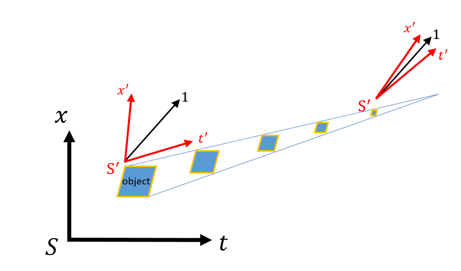
Figure 1: Schematic of S and $S^{\prime}$ coordinates in a movement framework

3 Mathematical Formulation

In this section, we make a mathematical formulation for the fractional dimensional basis vector and function. Before further processing, we demonstrate some important FDr definitions and determine a local FDr expression for some special functions in this study. Noted that in this study we have started with an approximation of the local part ($D^{\alpha}\Psi_{0}\approx\rm{local\ term}$) to build a mathematical framework for physics with fractional dimension point of view.

3.1 Definitions and a general framework

We describe an applicable mathematical tool for the purposes of this study by definitions of the basis functions for fractional domain by the realization of linear and fractional spaces.
Definition 1
Fractional space is a whole space between and included linear integer spaces.

Definition 2
If suppose the fractional space is a space between two consecutive integer dimensions, then the basis functions in the fractional space can be represented as a rotation of basis functions of the linear space.

Definition 3
The fractional derivative operator ($D_{t}^{\alpha}$) is a nonlocal operatore and there are several definitions for FDr such as direct, Riemann-Liouville (RL), Caputo (C), Liouville–Caputo and Fourier methods[9, 10]. The definition for RL and C FDr is expressed as follows

$$\begin{split}&{}_{a}^{RL}D_{t}^{\alpha}f(t)=\frac{1}{\Gamma(n-\alpha)}(\frac{d}{dt})^{n}\int_{a}^{t}(t-x)^{n-\alpha-1}f(x)dx,\\ &{}_{a}^{C}D_{t}^{\alpha}f(t)=\frac{1}{\Gamma(n-\alpha)}\int_{a}^{t}(t-x)^{n-\alpha-1}\frac{d^{n}f(x)}{dx^{n}}dx,\\ \end{split}$$ (5)

where $D^{\alpha}$, a, $\Gamma$ are the FDr operator of order $\alpha$, an initial point for integral and Gamma function, respectively.

Definition 4
The fractional derivative has two terms one common term and one extra term which is different depends on the type of FDr definition.

${}_{a}D_{t}^{\alpha}f(t)=\rm{common\ term+extra\ term=local\ term+nonlocal\ term}$.

There is an extra term as well as common one for every definitions presented for FDr based on the generalized hypergeometric function [10]. The common term is called a local fractional derivative because it can also be derived from an induction of integer derivative. Therefore, we call it local FDr.

Definition 5
The normalized FDr is a division of FDr over a normalization factor. Where normalization factor is an amplitude of FDr which is a function of $\alpha$. This makes confidence the normality of the basis functions holds.

Hint: For sake of simplicity and as a first investigation of fractional dimension in study physics, we continue with normalized local FDr part. The nonlocal part of fractional derivative can help us to explain a non-locality effect in physics. It is under further investigation and we will add more results about that in the future.

Normalized local FDr of some important functions
In this study, we need FDr of trigonometric, exponential and power series functions for further investigations. In this regard, we use the local term of FDr definition which is common for all definitions or from direct method by induction. Therefore, the following results are derived by a normalization of local FDr (LFDr) through a division by a normalization factor. More details are in the appendix.

$$\begin{split}&D_{\rm N,L}^{\alpha}\bigg{\{}{cos(\omega S)\bigg{\}}}=\frac{1}{D_{0}}D^{\alpha}\bigg{\{}{cos(\omega S)\bigg{\}}}=\frac{1}{D_{0}}(\omega)^{\alpha}cos(\omega S+\frac{\pi}{2}\alpha)=cos(\omega S+\frac{\pi}{2}\alpha),\\ &D_{\rm N,L}^{\alpha}\bigg{\{}{sin(\omega S)\bigg{\}}}=\frac{1}{D_{0}}D^{\alpha}\bigg{\{}{sin(\omega S)\bigg{\}}}=\frac{1}{D_{0}}(\omega)^{\alpha}sin(\omega S+\frac{\pi}{2}\alpha)=\sin(\omega S+\frac{\pi}{2}\alpha),\\ &D_{\rm N,L}^{\alpha}\bigg{\{}{e^{(i\omega S)}\bigg{\}}}=\frac{1}{D_{0}}D^{\alpha}\bigg{\{}{e^{(i\omega S)}\bigg{\}}}=\frac{1}{D_{0}}(\omega)^{\alpha}e^{(\omega S+\frac{\pi}{2}\alpha)}=e^{i(\omega S+\frac{\pi}{2}\alpha)},\end{split}$$ (6)

where $D_{\rm N,L}^{\alpha}$ and $D_{\rm 0}$ denote the normalized local FDr operator and the normalization factor, respectively. This make confidence the normality of the basis functions holds. $D_{0}$ denotes $(\omega)^{\alpha}$.
Local fractional derivative of a basic power function, $x^{n}$, can be derived from direct or Riemann–Liouville or Caputo or other methods with the same result[13]

$$D_{\rm N,L}^{\alpha}\bigg{\{}{x^{n}\bigg{\}}}=\frac{1}{D_{0}}D^{\alpha}\bigg{\{}{x^{n}\bigg{\}}}=\frac{1}{D_{0}}\frac{\Gamma(n+1)x^{(n-\alpha)}}{\Gamma(n-\alpha+1)}=x^{(n-\alpha)},$$ (7)

where $D_{0}$ is equal to $\frac{\Gamma(n-\alpha+1)}{\Gamma(n+1)}$.

Theorem 1
Let normalized LFDr operator applying in power series $(x^{n})$ and trigenometric functions ($e^{(i\omega S)}$), then this operator is a commutative and symmetry for these functions as follows:

$$D_{\rm N,L}^{\alpha_{1}}D_{\rm N,L}^{\alpha_{2}}=D_{\rm N,L}^{\alpha_{1}+\alpha_{2}},$$ (8)

$$D_{\rm N,L}^{\alpha}I_{\rm N,L}^{\alpha}=\mathds{1},$$ (9)

where the proof can be easily made for these functions as shown in the appendix.

3.1.1 Fractional Dimensional Basis Vector

Let $S$ and $S_{\alpha}$ are the basis vector of the linear and fractional spaces, respectively. Then, the relation between two coordinates regarding (7) is written as follows

$$S_{\alpha}=D_{\rm N,L}^{\alpha}\bigg{\{}{S\bigg{\}}}={S^{(1-\alpha)}}.$$ (10)

In conclusion, the coordinate $S_{\alpha}$ (red arrow) for a certain ${\alpha}$ as shown in Fig. 2 is a rotation of original coordinate S in fractional dimensional space. It can be derived from a LFDr operator with a certain order of ${\alpha}$.

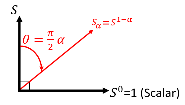
Figure 2: Schematic of fractional dimensional basic vector $S_{\alpha}$ (red arrow) from a rotation of integer basis vector S through FDr operator, a vector rotates from 0 dimension to 1 ($0\leq\alpha\leq 1$) or zero to 90 degrees rotation ($0\leq\theta\leq\frac{\pi}{2}$).

In Fig. 3, it is shown how a basic vector x through a rotation can reach 1. Scalar 1 is chosen because an integer derivative of x is equal to one. This will happen via a fractional derivative with the angle $\theta=\frac{\pi}{2}\alpha$. We need three orthogonal axes such as $x$ (representation of $x_{i}$), $t$ and $1$ as shown in Fig. 3(a) for depicting the fractional space of space-time, where two of them including $x$, $t$ are vector and $1$ denotes scalar one. Red colour arrows depicted in Fig. 3(b) to (d) show that space-time axes for $\alpha$ near to zero (Fig. 3(b)) mostly has a angle ($\theta$) near to zero, since $\alpha$ goes to one (Fig. 3(d)) the angle ($\theta$) is near to $\pi/2$.

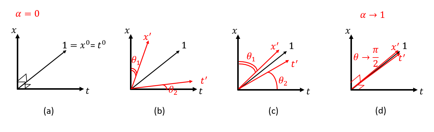
Figure 3: Rotation process of vector axes x and t through fractional space. (a) all vector axes are orthogonal ($\theta=0$ or $\alpha=0$), then by movement, the vector axes x and t will rotate: (b) $\theta\approx 0$ ($\alpha\approx 0$) , (c) $0<\theta<\pi/2$ ($0<\alpha<1$) and (d) $\theta\approx\pi/2$ ($\alpha\approx 1$).

As will shown in the next section, there are different scenarios depending on the angle rotation of $\theta$.

3.1.2 Fractional Dimensional Basis Function

Let $\phi(S)$ and $\phi_{\alpha}(S)$ be the basis functions of the linear and fractional spaces, respectively. Then, there are the following relations between the basis functions of both spaces:

$$\phi_{\alpha}(S)=D_{\rm N}^{\alpha}\bigg{\{}{\phi(S)\bigg{\}}}.$$ (11)

Note that $\alpha$ is a certain order of fractional dimension for each space-time position.

4 Preliminary plan

We limit our study to the three scenarios as shown in Table 1 due to having more general cases in physics. Note that most of the problems in physics can be covered by a trajectory with a maximum of quadratic order in fractional dimensional space for a moving system, as shown in Table 1.
The first is called static scenario when $\alpha$ is a constant value. The latter is a linear dynamic that corresponds to an inertial framework in physics. It will happen when $\alpha$ has a linear trajectory. The last is an accelerated system when the quadratic trajectory function acts. In this section, first of all, we discuss our attitude regarding dimension and then we investigate these three scenarios for both fractional dimensional basis vectors and functions. The trajectory function coefficients of $\alpha_{i}$, $\beta_{ij}$ and $\gamma_{ij}$ shown in Table 1 can be expressed in the format of a vector or matrix (tensor) depend on the trajectory of the fractional dimension.

Table.1:Different Observations
Scenario	Static	Linear Dynamic	Accelerated Dynamic
Trajectory ($\alpha_{i}(S)$)	$\alpha_{i}$	$\beta_{ij}S_{i}+\alpha_{i}$	$\gamma_{ijk}S_{j}S_{k}+\beta_{ij}S_{i}+\alpha_{i}$

4.1 Space-Dimension-Time

As we know, the concept of space-time comes from relativity theory and expresses that they coupled to each other for a moving system. However, there is a question of why they have coupled with each other even though it seems that they are independent. In this approach, there is an interconnection between space and time through the dimension we call it Space-Dimension-Time (SDT). In other words, space-time have been coupled to each other through the dimension where in Fig. 4 shows this interconnection. Although space and time are two independent variables, however; dimension through a dynamical movement interconnect them to each other.

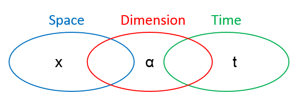
Figure 4: Space-time coupling through the dimension called Space-Dimension-Time (SDT)

There is no coupling in static scenario state since it is a steady one. To show a coupling between space and time, one could consider both of them as simple linear movement. Indeed, $x_{i}$ and t axes move rotationally toward scalar 1 axis. Being independent space and time asserts to us to write as follows

$$\begin{split}&\alpha_{i}(x_{i})=\beta_{i}x_{i}+\alpha_{i}\;\;(i=1,2,3),\\ &\alpha_{4}(t)=\beta_{4}t+\alpha_{4},\end{split}$$ (12)

taking an integer derivative

$$\begin{split}&d\alpha_{i}(x_{i})=\beta_{i}dx_{i},\\ &d\alpha_{4}(t)=\beta_{4}dt,\end{split}$$ (13)

and then by dividing of them, we have

$$\begin{split}\frac{d(\alpha_{i}(x_{i}))}{d(\alpha_{4}(t))}=\frac{\beta_{i}dx_{i}}{\beta_{4}dt}=\frac{\beta_{i}}{\beta_{4}}v_{i}.\end{split}$$ (14)

The relation (14) says us when moving with a constant speed, movement of rotational variable x-axis toward t one has a relation to speed. In other words, space is related to time when looking at it from dimensional point of view.

4.2 Presentation of Static and Moving Coordinate Systems via Fractional Dimensional Basis Vector

Besides static case, there are two important types of dynamic systems in physics either movement of constant velocity or acceleration. These types of systems in our study correspond to an angle rotation of coordinate $S_{\alpha}$ of a linear rotation (constant velocity) or quadratic rotation (constant acceleration). It should be noted that if two coordinates of $S$ and $S_{\alpha}$ are lying with each other, then $\alpha$ is equal to zero or $\theta=0$ and when they are so far from each other $\alpha$ is going to 1 ($\theta\to\frac{\pi}{2}$). This property is independent of the type of dynamic system. It means that S and $S_{\alpha}$ are lying each other for both accelerated and inertial framework systems when $\alpha$ is equal to zero and when two coordinates are faring away for both systems $\alpha$ is going to 1.

4.2.1 Static scenario

In this case, two coordinates S and $S_{\alpha}$ are considered to be fixed. Therefore, there is a constant space distance ($S_{\rm offset}$) between a fixed observer and static framework. It should be noted that the space distance offset is equal to $|S_{\rm offset}|=\sqrt{x_{1,\rm offset}^{2}+x_{2,\rm offset}^{2}+x_{3,\rm offset}^{2}}$ and time distance offset can be zero for static case, however; it is not valid for dynamic scenario because we have space-time distance or in this aspect SDT distance. To find $\alpha$, it is needed to define an infinite space parameter ($|S_{\infty}|$). Infinite space (time) parameter ($|S_{\infty}|$) is a certain value of space (time) where after that the observer (camera) can not measure the observed framework anymore and it disappears from the observer point of view ($|S_{\rm\infty}|=\sqrt{x_{1,\rm\infty}^{2}+x_{2,\rm\infty}^{2}+x_{3,\rm\infty}^{2}}$). Therefore, $\alpha$ for a static scenario can be realized as follows

$$\alpha=\frac{|S_{\rm offset}|}{|S_{\infty}|}=\alpha_{0}.$$ (15)

So, the fractional dimensional basis vector is

$$S_{\alpha}=D_{\rm N,L}^{\alpha_{0}}\big{\{}{S\big{\}}}.$$ (16)

Different situations for static observation are tabulated in Table 1. When two coordinates are lying each other the $S_{\rm offset}$ is equal to zero resulting $\alpha=0$ ($S=S_{\alpha}$). If $S_{\rm offset}$ has a value larger than zero and smaller than $S_{\infty}$, thus we have an $\alpha_{0}$ in a range between zero and one ( $0<\alpha_{0}<1$) and when two coordinates are very far each other $S_{\rm offset}\to S_{\infty}$ which leads to $\alpha\to 1$. For instance, imagine one object is in front of the observer, then $S_{\rm offset}=0$ and therefore $\alpha=\alpha_{0}=0$. Now, we put the same object with a distance of $S_{\rm offset}=\frac{1}{2}S_{\infty}$ and then from the same observer the $\alpha=\alpha_{0}=0.5$. It must be mentioned when $S_{\rm offset}>S_{\infty}$ the measurement is not correct due to disappearing the observed framework from the observer and leads to high error tolerance.

Table.1:Different Situations for Static Observation
$S_{\rm offset}$	$S_{\rm offset}=0$	$0<S_{\rm offset}<S_{\infty}$	$S_{\rm offset}\to S_{\infty}$	$S_{\rm offset}>S_{\infty}$
$\alpha=\alpha_{0}$	$\alpha_{0}=0$	$0<\alpha_{0}<1$	$\alpha_{0}\to 1$	$\alpha_{0}>1$
Measurement	$\checkmark$	$\checkmark$	$\checkmark$	$\times$

4.2.2 Linear and Quadratic Dynamic

A Moving system leads to a rotation of coordinate depends on the function trajectory in space-time from fractional dimensional point of view. To sake of simplicity, linear and quadratic trajectories of moving coordinate are chosen. Then, we find an equivalent physical problem for that. In physics, when we have inertial framework (constant speed), special relativity and Minkowski space are used, and when we have accelerated frames (constant acceleration or gravity), general relativity and Riemann space are used. With a physical counterpart, we should obtain the same result with special relativity when $\alpha$ has a linear trajectory and general relativity when $\alpha$ has a quadratic trajectory.

Further investigations need a new metric for fractional dimensional space-time or SDT. It is out of this study and we will consider it as a future work, however; we try to express an equivalency of our model with some simplified examples. We can represent a $S^{\prime}$ coordinate based on the trigonometric properties as following

$$\begin{split}\begin{pmatrix}x_{1}^{\prime}\\ x_{2}^{\prime}\\ x_{3}^{\prime}\\ t^{\prime}\end{pmatrix}=\begin{pmatrix}cos\big{(}\theta_{1}(S)\big{)}&0&0&0\\ 0&cos\big{(}\theta_{2}(S)\big{)}&0&0\\ 0&0&cos\big{(}\theta_{3}(S)\big{)}&0\\ 0&0&0&cos\big{(}\theta_{4}(S)\big{)}\\ \end{pmatrix}\begin{pmatrix}x_{1}\\ x_{2}\\ x_{3}\\ t\end{pmatrix}+\begin{pmatrix}sin\big{(}\theta_{1}(S)\big{)}\\ sin\big{(}\theta_{2}(S)\big{)}\\ sin\big{(}\theta_{3}(S)\big{)}\\ sin\big{(}\theta_{4}(S)\big{)}\end{pmatrix},\end{split}$$ (17)

where $\theta_{i}(S)$ (i=1,2,3,4) is equal to $\frac{\pi}{2}\alpha_{i}(S)$. As an example we consider a situation for very slow motion of an inertial framework in direction of $x_{1}$ where $\theta_{1}$ is very small ($cos\theta_{1}\approx 1$ and $sin\theta_{1}\approx\theta_{1}$) and $\theta_{2}=\theta_{3}=\theta_{4}=0$. Therefore the coordinate transformation can be approximated to Galilean transformation with $sin\theta_{1}\approx\pm vt$.

$$\begin{split}\begin{pmatrix}x_{1}^{\prime}\\ x_{2}^{\prime}\\ x_{3}^{\prime}\\ t^{\prime}\end{pmatrix}=\begin{pmatrix}1&0&0&0\\ 0&1&0&0\\ 0&0&1&0\\ 0&0&0&1\\ \end{pmatrix}\begin{pmatrix}x_{1}\\ x_{2}\\ x_{3}\\ t\end{pmatrix}+\begin{pmatrix}\pm vt\\ 0\\ 0\\ 0\end{pmatrix}.\end{split}$$ (18)

Similarly, for an accelerated system in $x_{1}$ or $x^{\prime}_{1}$ direction with a small acceleration or gravity and an approximation of $sin\theta_{1}\approx\theta_{1}=\pm\frac{1}{2}gt^{2}$ and $\theta_{2}=\theta_{3}=\theta_{4}=0$, the coordinate transformation can be expressed as follows

$$\begin{split}\begin{pmatrix}x_{1}^{\prime}\\ x_{2}^{\prime}\\ x_{3}^{\prime}\\ t^{\prime}\end{pmatrix}=\begin{pmatrix}1&0&0&0\\ 0&1&0&0\\ 0&0&1&0\\ 0&0&0&1\\ \end{pmatrix}\begin{pmatrix}x_{1}\\ x_{2}\\ x_{3}\\ t\end{pmatrix}+\begin{pmatrix}\pm\frac{1}{2}gt^{2}\\ 0\\ 0\\ 0\end{pmatrix}.\end{split}$$ (19)

4.3 A Signal Representation of System via Fractional Dimensional Basis Function

In this section, we demonstrate the signal behavior based on the three scenarios. By the use of assumption (11), we can also rewrite the formulation between basis function of transmitter ($T(S)$) and receiver ($R(S)$) signals as follows

$$R(S)=\frac{1}{2}D_{\rm N}^{\alpha}\big{\{}{T(S)\big{\}}}+\frac{1}{2}\bigg{(}D_{\rm N}^{\alpha}\big{\{}{T(S)\big{\}}}\bigg{)}^{*}=Re\bigg{\{}{D_{\rm N}^{\alpha}\big{\{}{T(S)\big{\}}}\bigg{\}}},$$ (20)

where $\Re$ is real part of basis function. The FDr operator connects the input signal (initial signal) to the output signal of the system through a trajectory in fractional dimension. This assumption denotes that the transmitter itself is in an integer coordinate, however; from receiver point of view has a fractional dimensional coordinate.
Note that for the sake of simplicity we play with two variables $x_{1}$ (space) and t (time) where $x_{1}$ is symbolized by $z$. So hereafter, $z$ and t denote space and time variables, respectively.

4.3.1 Static scenario

From signal point of view , a constant distance holds between transmitter and receiver as shown in Fig. 5 (a). This is like that an observer see a standing object from a certain fixed distance.

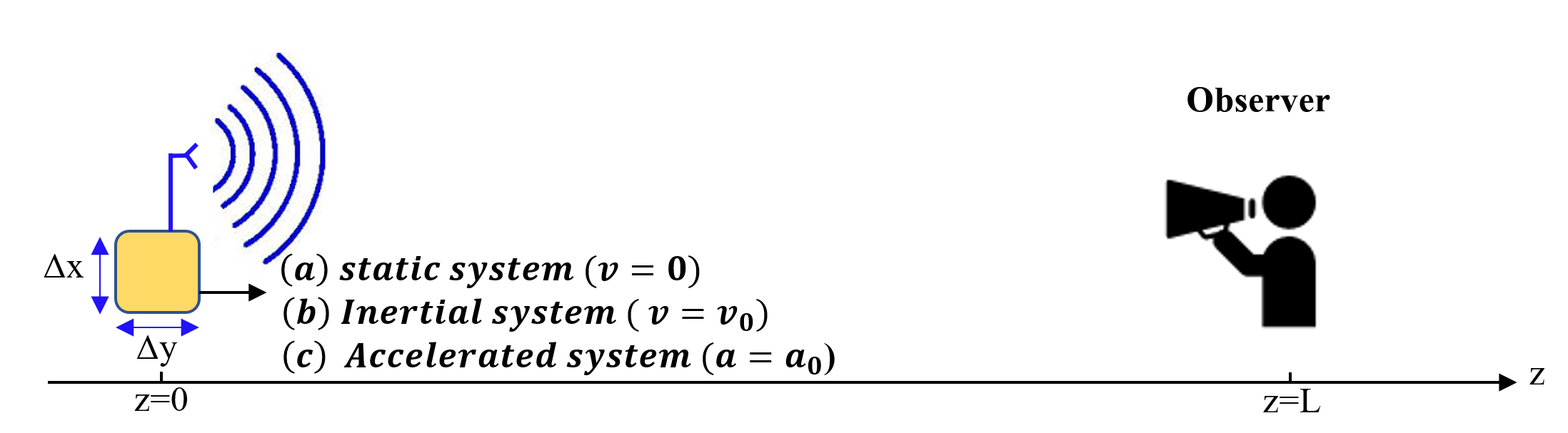
Figure 5: Schematic of three scenarios (a) static ($v=0$) (b) Linear dynamic ($v=v_{0}$) (c) accelerated system ($a=a_{0}$)

For example, a signal of formula $A_{0}cos(\omega t+kz)$ is propagating in free space . How is the received signal diagram change $(R(z=L,t))$ after a propagation of distance L in a (a) lossless (b) lossy medium? Where $A_{0}$, $\omega$ and $k$ are amplitude, angular frequency and wave vector, respectively.
Hint: when electromagnetic wave is propagating in a lossy medium, wave vector is a complex value as

$$k=\beta+i\alpha_{att.},$$ (21)

where $\beta$ and $\alpha_{att.}$ are propagation constant and attenuation decay coefficient.
The answer for part (a) is:
from electrodynamics side, we know that the signal has a phase shift corresponding to $kL$ where in lossless medium $k$ is equal to propagation constant $\beta$.

$$R(z=L,t)=A_{0}cos(\omega t+\beta L)=A_{0}cos(\omega t+\Phi),$$ (22)

where $\Phi$ is equal to $\beta L$.
However from fractional dimensional point of view, the received signal at $z=L$ is obtained by a constant fractional dimension of $\alpha_{0}$. Therefore, we have

$$R(z=L,t)=D_{\rm N,L}^{\alpha_{0}}\big{\{}{A_{0}cos(\omega t)\big{\}}}=A_{0}cos(\omega t+\frac{\pi\alpha_{0}}{2})=A_{0}cos(\omega t+\Phi),$$ (23)

where $\Phi=\beta L=\frac{\pi\alpha_{0}}{2}$.
and the answer for part (b) is:
from electrodynamics aspect, the final received signal after a simplification at the distance L is

$$R(z=L,t)=A_{0}e^{-\alpha_{att.}L}cos(\omega t+\beta L),$$ (24)

and from fractional dimensional perspective, we have

$$R(z=L,t)=\frac{1}{2}D_{\rm N,L}^{\alpha_{0}}\big{\{}{e^{i\omega t}\big{\}}}+\frac{1}{2}\bigg{(}D_{\rm N,L}^{\alpha_{0}}\big{\{}{e^{i\omega t}\big{\}}}\bigg{)}^{*}=\frac{1}{2}D_{\rm N,L}^{\alpha_{0}}\big{\{}{e^{i\omega t}\big{\}}}+\frac{1}{2}\bigg{(}D_{\rm N,L}^{\alpha^{*}_{0}}\big{\{}{e^{-i\omega t}\big{\}}}\bigg{)},$$ (25)

where $\alpha_{0}$ has a complex value as follows

$$\alpha_{0}=\alpha^{\rm R}_{0}+i\alpha^{\rm I}_{0}.$$ (26)

Then, the complex fractional basis function is

$$D_{\rm N,L}^{\alpha_{0}}\big{\{}{e^{i\omega t}\big{\}}}=e^{i(\omega t+\frac{\pi\alpha_{0}}{2})}=e^{i(\omega t+\frac{\pi}{2}\alpha^{\rm R}_{0}+i\frac{\pi}{2}\alpha^{\rm I}_{0})}=e^{(-\frac{\pi}{2}\alpha^{\rm I}_{0})}e^{i(\omega t+\frac{\pi}{2}\alpha^{\rm R}_{0})},$$ (27)

where $D_{\rm N,L}^{\alpha_{0}^{*}}\big{\{}{e^{-i\omega t}\big{\}}}$ is equal to the complex conjugate of $D_{\rm N,L}^{\alpha_{0}}\big{\{}{e^{i\omega t}\big{\}}}$. Thus, after a rearrangement we have

$$R(z=L,t)=A_{0}\Re\bigg{\{}{D_{\rm N,L}^{\alpha_{0}}(\big{\{}{e^{i\omega t}\big{\}}}\bigg{\}}}=A_{0}e^{-(\frac{\pi}{2}\alpha^{\rm I}_{0})}cos(\omega t+\frac{\pi}{2}\alpha^{\rm R}_{0}),$$ (28)

It can be observed that decaying a signal as loss in linear vector space corresponds to a trajectory of signal in imaginary domain of fractional dimension. Therefore, we have:

$$\frac{\pi}{2}\alpha^{\rm R}_{0}=\beta L,$$ (29)

and

$$\frac{\pi}{2}\alpha^{\rm I}_{0}=\alpha_{att.}L.$$ (30)

4.3.2 Dynamic Scenario

In this case, at least one of the transmitter or receiver is moving in fractional dimensions. Therefore, it is called dynamic observation. Here, two types of movement of linear and quadratic trajectories are demonstrated.

4.3.2.1   Linear dynamic

We show that the two important cases in physics such as wave equation and Doppler effect are equivalent to a movement system in fractional dimensional space with a linear trajectory.

4.3.2.1.1 Equivalency for the Wave Equation

We start to reformulate a new representation of the wave equation based on the proposed assumption. As we know, wave is a phenomenon in time which exactly propagates in the space. It can be corresponded to a temporal (spatial) signal moving in spatial (temporal) domain with a fractional dimensional trajectory of $\alpha(\bf r)$ ($\alpha(t)$). The wave function (${\bf\Psi}(\bf{r}$,$t))$ can be decomposed into the two independently variable functions of $t$ and space variables $\bf{r}$ (${\bf{\Psi}}$ $(\bf{r}$$,t)$$=\psi_{1}(t)\psi_{2}(\bf{r})$). Therefore, the wave equation can be realized as follows

$$D_{\rm N}^{\alpha_{1}(\bf r)}\bigg{\{}{{\bf\psi_{1}}(t)\bigg{\}}}=D_{\rm N}^{\alpha_{2}(t)}\bigg{\{}{\{{\bf\psi_{2}}(\bf r)\bigg{\}}}.$$ (31)

The left hand side of (31) means that temporal signal ($\psi_{1}(t)$) moves in spatial domain with a trajectory of $\alpha_{1}(\bf r)$ and has to be equal to the right one of equation where it shows the movement of spatial signal ($\psi_{2}(\bf{r})$ in time domain with a trajectory of $\alpha_{2}(t)$. For sake of simplicity as we know from quantum or electrodynamics, the wave basis function of two variables $z$ and $t$ (${\bf\Psi}(\bf{z}$,$t)$) is equal to $e^{i(\omega t+kz)}$. Thus, the fractional dimensional wave equation is

$$D_{\rm N,L}^{\alpha_{1}(z)}\bigg{\{}{e^{i\omega t}\bigg{\}}}=D_{\rm N,L}^{\alpha_{2}(t)}\bigg{\{}{e^{ikz}\bigg{\}}}=e^{i(\omega t+\frac{\pi}{2}\alpha_{1}(z))}=e^{i(kz+\frac{\pi}{2}\alpha_{2}(t))}=e^{i(\omega t+kz)},$$ (32)

where trajectories of $\alpha_{i}$ (i=1,2) are

$$\begin{split}\alpha_{1}(z)=\frac{2}{\pi}kz\\ \alpha_{2}(t)=\frac{2}{\pi}\omega t,\end{split}$$ (33)

4.3.2.1.2 Doppler effect

As shown in Fig.5 (b) for an inertial system, an observer has stayed in a certain fixed position (here $z=L$) and the transmitter is closing (faring away) to the receiver with a velocity of $v_{t}$. This phenomenon is well-known in physics and called the Doppler effect. Here, it is shown how the movement of the signal source with a linear trajectory in fractional dimension is equivalent to the Doppler effect. Let us to have a signal, $T(z=0,t)$, at transmitter of the following expression

$$T(z=0,t)=A_{0}cos(\omega t).$$ (34)

Therefore, by considering the trajectory as follows

$$\alpha(z,t)=\beta_{41}z+\beta_{44}t,$$ (35)

where $\beta_{41}$ and $\beta_{44}$ constant coefficients and letting $z$ as a constant value vs. t, the received signal is

$$R(z=L,t)=D_{\rm N,L}^{\alpha(S)}\bigg{\{}{A_{0}cos(\omega t)\bigg{\}}}=A_{0}cos(\omega t+\frac{\pi\alpha(S)}{2})=A_{0}cos(\omega t+\frac{\pi(\beta_{41}z+\beta_{44}t)}{2}).$$ (36)

After a rearrangement, it is

$$R(z=L,t)=A_{0}cos(\omega_{D}t+\Phi),$$ (37)

where constant phase is

$$\begin{split}\Phi=\frac{\pi}{2}\beta_{41}L,\end{split}$$ (38)

and $\omega_{D}$ is a new (Doppler) angular frequency.

$$\begin{split}\omega_{D}=\omega+\frac{\pi\beta_{44}}{2}=2\pi(f+\Delta f)=2\pi f_{D},\end{split}$$ (39)

with Doppler frequency shift [16]

$$\begin{split}f_{D}=\bigg{(}\frac{c\pm v_{r}}{c\pm v_{t}}\bigg{)}f=f+\bigg{(}\frac{\pm v_{r}\mp v_{t}}{c\pm v_{t}}\bigg{)}f=f+\Delta f,\end{split}$$ (40)

where c is the propagation speed of wave in the medium. When the receiver is moving towards (away) the source, the sign is positive (negative). For this scenario observer velocity ($v_{r}$) is zero ($v_{r}=0$), and $\Delta f$ is:

$$\begin{split}\Delta f=\bigg{(}\frac{\mp v_{t}}{c\pm v_{t}}\bigg{)}f=\frac{\beta_{44}}{4}.\end{split}$$ (41)

4.3.3 Acceleration dynamic scenario

In this case, trajectory in fractional dimension is a quadratic function. Here, we assumed the following trajectory

$$\alpha(S)=\alpha(z,t)=\gamma_{41}z^{2}+\gamma_{44}t^{2}+\beta_{41}z+\beta_{44}t,$$ (42)

where $\beta_{41}$, $\beta_{44}$, $\gamma_{41}$ and $\gamma_{44}$ constant coefficients where with zeroing the $\gamma$ coefficients the Doppler problem will be obtained. Therefore, the basis function for accelerated system can be presented as follows

$$\phi^{\alpha(z,t)}(S)=D_{\rm N}^{(\gamma_{41}z^{2}+\gamma_{44}t^{2}+\beta_{41}z+\beta_{44}t)}\bigg{\{}{\phi(S)\bigg{\}}},$$ (43)

and the received signal regarding being constant $z$ vs. t is

$$\begin{split}&R(z,t)=D_{\rm N,L}^{\alpha(z,t)}\bigg{\{}{A_{0}cos(\omega t)\bigg{\}}}=A_{0}cos(\omega t+\frac{\pi\alpha(z,t)}{2})\\ &=A_{0}cos(\omega t+\frac{\pi(\gamma_{41}z^{2}+\gamma_{44}t^{2}+\beta_{41}z+\beta_{44}t)}{2}).\end{split}$$ (44)

After a rearrangement, it is

$$R(z=L,t)=A_{0}cos(\omega_{Da}(t)t+\Phi),$$ (45)

where constant phase at $z=L$ is

$$\begin{split}\Phi=\frac{\pi}{2}(\gamma_{14}L^{2}+\beta_{14}L)\end{split}$$ (46)

and $\omega_{Da}(t)$ is a new (Doppler) angular time dependent as follows

$$\begin{split}\omega_{Da}(t)=\frac{\pi\gamma_{44}}{2}t+\omega+\frac{\pi\beta_{44}}{2}=\frac{\pi\gamma_{44}}{2}t+\omega_{D}.\end{split}$$ (47)

It is corresponded with the gravitational red (blue)-shift. As a simple example, the profile of (47) with all coefficients normalized to one is depicted in Fig. 6. It can be observed that its profile shows a gravitational red (blue)-shift behavior [17] and also without consideration of envelope, it has a similar behavior like gravitational wave [18].

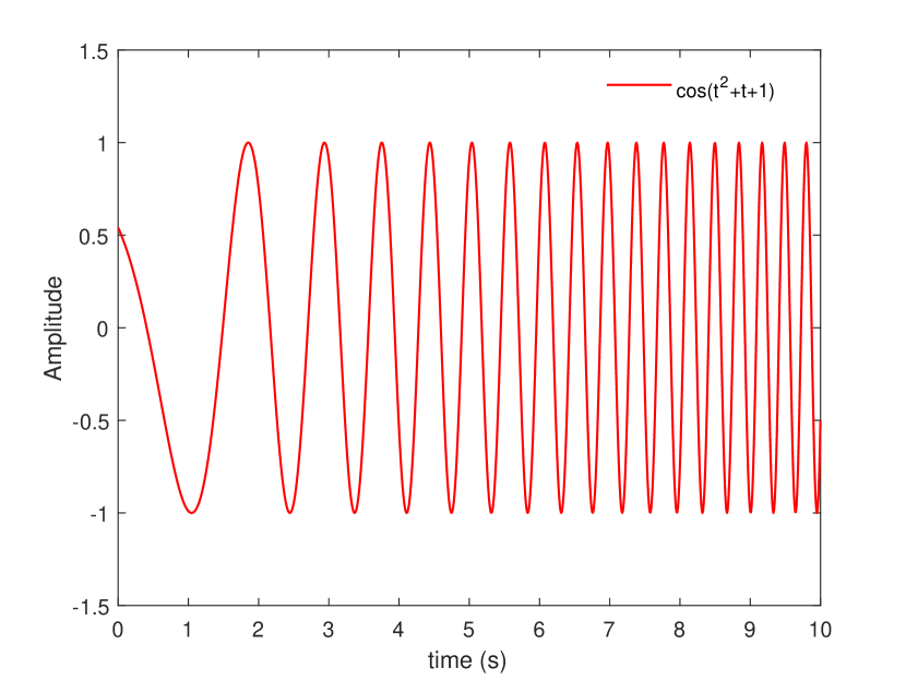
Figure 6: The plot of cosine function with quadratic trajectory in fractional dimension.

5 Acknowledgement

The author is very appreciate for fruitful discussion with A. Sabihi and his valuable comments.

6 Appendix

6.1 Proof Theorem 1

Let normalized LFDr operator applying in power series $(x^{n})$ and trigenometric function ($e^{(i\omega S)}$), then this operator is a commutative and symmetry for these function as follows:

$$D_{\rm N,L}^{\alpha_{1}}D_{\rm N,L}^{\alpha_{2}}=D_{\rm N,L}^{\alpha_{1}+\alpha_{2}},$$ (48)

$$D_{\rm N,L}^{\alpha}I_{\rm N,L}^{\alpha}=\mathds{1},$$ (49)

Proof
We can start with cosine function and applying in the left hand side of Eq. (48):

$$D_{\rm N,L}^{\alpha_{1}}D_{\rm N,L}^{\alpha_{2}}\bigg{\{}{cos(\omega S)\bigg{\}}}=D_{\rm N,L}^{\alpha_{1}}\bigg{\{}{cos(\omega S+\frac{\pi}{2}\alpha_{2})\bigg{\}}}=cos(\omega S+\frac{\pi}{2}\alpha_{2}+\frac{\pi}{2}\alpha_{1}),$$ (50)

then for the right side we have :

$$D_{\rm N,L}^{\alpha_{1}+\alpha_{2}}\bigg{\{}{cos(\omega S)\bigg{\}}}=cos(\omega S+\frac{\pi}{2}(\alpha_{1}+\alpha_{2})).$$ (51)

Therefore, they are equivalent and with the same analogy it is consistent for the sinus , complex basis and power series functions.
For the proof of Eq. (49), firstly we have to mentioned that the fractional integral of order $\alpha$ ($I_{\rm N,L}^{\alpha}$) of an arbitrary function $f$ can be expressed based on the FDr.

$$I_{\rm N,L}^{\alpha}f=D_{\rm N,L}^{-\alpha}f.$$ (52)

Then, we have

$$D_{\rm N,L}^{\alpha}I_{\rm N,L}^{\alpha}\bigg{\{}{cos(\omega S)\bigg{\}}}=D_{\rm N,L}^{\alpha}\bigg{\{}{cos(\omega S-\frac{\pi}{2}\alpha)\bigg{\}}}=cos(\omega S+\frac{\pi}{2}\alpha-\frac{\pi}{2}\alpha)=cos(\omega S),$$ (53)

and it can be applied for the other proposed functions.

6.2 Fractional Dimensional Basis Vector

There is another approach to reach the same result as presented in Eq. (10). When the relation between two coordinates of S and $S_{\alpha}$ can be expressed based on the superposition of FDr (order of $\alpha$) of S coordinate in one hand and the fractional integral (order of $\beta=1-\alpha$) of 1 on the other hand. It should be noted that summation of order of fractional operators has to be one since it should correspond to 90 degree rotation.

$$\begin{split}S_{\alpha}=(1-\alpha)D_{\rm N,L}^{\alpha}\{{S\}}+\alpha I_{\rm N,L}^{\beta}\{{1\}}=(1-\alpha)D_{\rm N,L}^{\alpha}\{{S\}}+\alpha D_{\rm N,L}^{-\beta}\{{1\}}.\end{split}$$ (54)

Where the coefficients of $D{\rm N,L}^{\alpha}$ and $I{\rm N,L}^{\alpha}$ as weight factors are $(1-\alpha)$ and $(\alpha)$, respectively. These weight factors have been considered for the satisfaction of rotation coordinate when the trajectory ($\alpha(S)$) is equal to zero both coordinates of $S$ and $S_{\alpha}$ are lying each other and when $\alpha$ is equal to one, it leads to 90 degree rotation of S coordinate in fractional dimension space and will be 1. Therefore, $S_{\alpha}$ coordinate is

$$\begin{split}S_{\alpha}=(1-\alpha)S^{1-\alpha}+\alpha S^{1-\alpha}=S^{1-\alpha}.\end{split}$$ (55)

6.3 Example

For more clarification, the 3-D plot of FDr of function f(x)=x for an interval x between [0,10] and $\alpha$ between [0,1] are depicted in Fig.6.

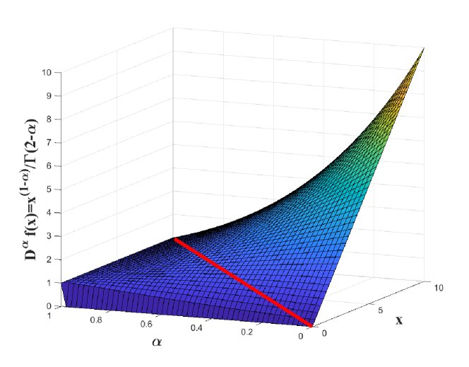
Figure 7: FDr of function f(x)=x for interval of [0,10] and alpha between zero and one.

We wish to see choosing a trajectory on the red line in Figure 6 how the FDr diagram does change? The red line corresponds to a trajectory of $\alpha=.1x$ which leads to the FDr plot on the proposed trajectory as shown in Fig. 7. It means for every point of x, there is a special $\alpha$ which makes a function of $\alpha(x)$.

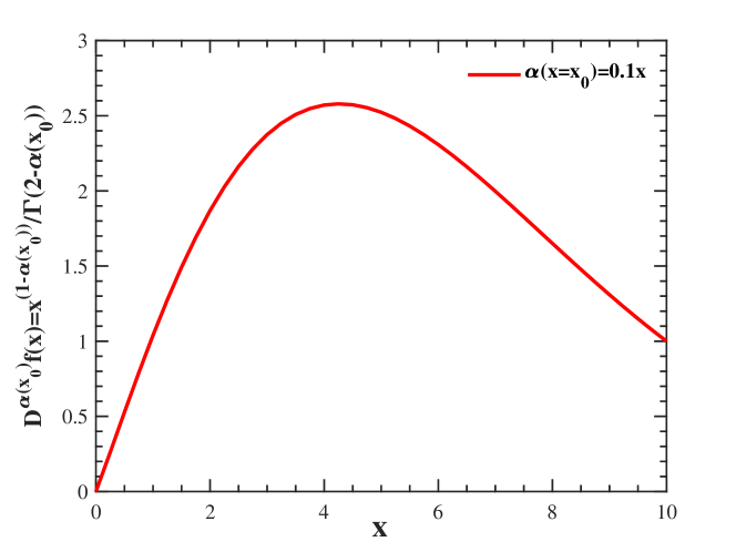
Figure 8: FDr of function f(x)=x for interval of [0,10] for the trajectory of $\alpha=.1x$. It should be noted that for every point of x we have a special constant value of $\alpha$.

References

- [1] R. M. Smullyan, Gödel’s incompleteness theorems (Oxford University Press on Demand, 1992).
- [2] R. M. Wald, General relativity (University of Chicago press, 2010).
- [3] A. Galindo and P. Pascual, Quantum mechanics I (Springer Science and Business Media, 2012).
- [4] K. Becker, M. Becker, and J. H. Schwarz, String theory and M-theory: A modern introduction (Cambridge university press, 2006).
- [5] B. R. Holstein, “Graviton physics,” Am. J. physics 74, 1002–1011 (2006).
- [6] A. Dorostkar and A. Sabihi, “Fourier series in fractional dimensional space,” arXiv preprint arXiv:2212.00049 (2022).
- [7] Baer, Reinhold. Linear algebra and projective geometry. Courier Corporation, 2005.
- [8] Hilbert, David, and Stephan Cohn-Vossen. Geometry and the Imagination. Vol. 87. American Mathematical Soc., 2021.
- [9] G. Shchedrin, N. Smith, A. Gladkina, and L. Carr, “Exact results for a fractional derivative of elementary functions,” SciPost Phys. 4, 029 (2018).
- [10] R. Herrmann, Fractional calculus: an introduction for physicists (World Scientific, 2011).
- [11] https://math.stackexchange.com/questions/1593339/how-do-you-take-the-fractional-derivative-j-frac12fx-where-fx-w-sin.
- [12] M. Chen, S. Shao, and P. Shi, Robust adaptive control for fractional-order systems with disturbance and saturation (John Wiley and Sons, 2017).
- [13] K. Oldham and J. Spanier, The fractional calculus theory and applications of differentiation and integration to arbitrary order (Elsevier, 1974).
- [14] , S. Mazzucchi, Mathematical Feynman path integrals and their applications,(World Scientific,2009)
- [15] Albeverio, Sergio, and Sonia Mazzucchi. "Generalized fresnel integrals." Bulletin des sciences mathematiques 129.1 (2005): 1-23.
- [16] V. C. Chen, The micro-Doppler effect in radar (Artech house, 2019).
- [17] A. Eddington, “Einstein shift and doppler shift,” Nature 117, 86–86 (1926).
- [18] W. G. Anderson and J. D. Creighton, Gravitational-wave physics and astronomy: An introduction to theory, experiment and data analysis (John Wiley and Sons, 2012).