Identifying Adversarially Attackable and Robust Samples

Abstract

Adversarial attacks insert small, imperceptible perturbations to input samples that cause large, undesired changes to the output of deep learning models. Despite extensive research on generating adversarial attacks and building defense systems, there has been limited research on understanding adversarial attacks from an input-data perspective. This work introduces the notion of sample attackability, where we aim to identify samples that are most susceptible to adversarial attacks (attackable samples) and conversely also identify the least susceptible samples (robust samples). We propose a deep-learning-based detector to identify the adversarially attackable and robust samples in an unseen dataset for an unseen target model. Experiments on standard image classification datasets enables us to assess the portability of the deep attackability detector across a range of architectures. We find that the deep attackability detector performs better than simple model uncertainty-based measures for identifying the attackable/robust samples. This suggests that uncertainty is an inadequate proxy for measuring sample distance to a decision boundary. In addition to better understanding adversarial attack theory, it is found that the ability to identify the adversarially attackable and robust samples has implications for improving the efficiency of sample-selection tasks. Link to code: https://github.com/rainavyas/img_attackability

1 Introduction

Deep learning models have achieved remarkable success across a wide range of tasks and domains, including image classification (He, 2020) and natural language processing (Khurana et al., 2017). However, these models are also susceptible to adversarial attacks (Goodfellow et al., 2014), where small, imperceptible perturbations to the input can cause large, undesired changes to the output of the model (Serban et al., 2020; Zhang et al., 2019; Huynh et al., 2022). Extensive research has been conducted on generating adversarial attacks and building defense systems (Biggio & Roli, 2017; Chakraborty et al., 2018), such as detection (Shen et al., 2019; Raina & Gales, 2022; Shaham et al., 2018; Hendrycks & Gimpel, 2016; Smith & Gal, 2018) or adversarial training (Qian et al., 2022; Bai et al., 2021; Muhammad & Bae, 2022). However, little or no work has sought to understand adversarial attacks from an input-data perspective. In particular, it is unclear why some samples are more susceptible to attacks than others. Some samples may require a much smaller perturbation for a successful attack (attackable samples), while others may be less susceptible to imperceptible attacks and require much larger perturbations (robust samples). Determining the attackability of samples can have important implications for various tasks, such as active learning (Ren et al., 2020; Sun & Wang, 2010) and adversarial training (Qian et al., 2022). In the field of active learning, adversarial perturbation sizes can be used by the acquisition function to select the most useful/uncertain samples for training (Ducoffe & Precioso, 2018; Ru et al., 2020). Similarly, adversarial training can be made more efficient by augmenting with adversarial examples for only the most attackable samples to avoid unnecessarily scaling training times, i.e. a variant of weighted adversarial training (Holtz et al., 2022).

This work defines the notion of sample attackability: the smallest perturbation size required to change a sample’s output prediction. To determine if a particular sample is attackable or robust, we use the imperceptibility threshold in the definition of an adversarial attack. In automated adversarial attack settings, a proxy function is often used to measure human perception (Sen et al., 2020) and thus there can be a range of acceptable thresholds for the imperceptibility boundary, as per the proxy measure. In this work, If a sample’s minimum perturbation size is within a strict threshold of imperceptibility, then the sample is considered an adversarially attackable sample. In converse, a sample with a perturbation size greater than a much more generous threshold for imperceptibility is termed as robust. Further, this work proposes a simple deep-learning based detector to identify the attackable and robust samples, agnostic to a specific model’s realisation or architecture. The attackability detector is evaluated on an unseen dataset, for an unseen target model. Further, the attackability detector is evaluated with unmatched adversarial attack methods; i.e. the detector is trained using perturbation sizes defined by the simple Finite Gradient Sign Method (FGSM) attack (Goodfellow et al., 2014), but evaluated on sample perturbation sizes calculated using for example a more powerful Project Gradient Descent (PGD) attack method (Madry et al., 2017). The deep-learning based attackability detector is also compared to alternative uncertainty (Kim et al., 2021; Gawlikowski et al., 2021) based detectors.

2 Related Works

Sample Attackability: Zeng et al. (2020) introduce the notion of sample attackability through the language of vulnerability of a sample to an adversarial attack. Kim et al. (2021) further consider sample vulnerability by using model entropy to estimate how sensitive a sample may be to adversarial attacks. This uncertainty approach is considered as a baseline in this work.

Understanding adversarial samples: For understanding sample attackability, it is useful to consider adversarial attack explanations from the data perspective. Initial explanations (Szegedy et al., 2013; Gu & Rigazio, 2014) argued that adversarial examples lie in large and continuous pockets of the data manifold (low-probability space), which can be easily accessed. Conversely, it is also hypothesized (Tanay & Griffin, 2016) that adversarial examples simply lie in low variance directions of the data, but this explanation is often challenged (Izmailov et al., 2018). Similarly, many pieces of work (Song et al., 2017; Meng & Chen, 2017; Lee et al., 2017; Ghosh et al., 2018) argue that adversarial examples lie orthogonal to the data manifold and can so can easily be reached with small perturbations. It can also be argued (Gilmer et al., 2018) that adversarial examples are a simple consequence of intricate and high-dimensional data manifolds.

Use of adversarial perturbations: In the field of active learning (Ren et al., 2020; Sun & Wang, 2010), methods have been proposed to exploit adversarial attacks to determine the minimum perturbation size. The perturbation size is a proxy for distance to a model’s decision boundary and thus an acquisition function selects the samples with the smallest perturbations for training the model. However, in these works the perturbation sizes are specific to the model being trained, as opposed to contributing to the overall measure of the attackability of a sample, agnostic of the model and adversarial attack method.

Weighted Adversarial Training Knowledge of sample attackability can be applied to the field of adversarial training. Adversarial training (Qian et al., 2022) is a popular method to enhance the robustness of systems, where a system is trained on adversarial examples. However, certain adversarial examples can be more useful than others and hence certain research attempts have explored reweighing of adversarial examples during training. For example, the adversarial training loss function can be adapted to give greater importance to capture an adversarial example’s class margin (Holtz et al., 2022). Alternatively, adversarial examples can be re-weighted using the model confidence associated with each example (Zeng et al., 2020). However, as opposed to considering the full set of generated adversarial examples, it is more useful to determine which original/non-adversarial samples it is worth using to generate an adversarial example for the purpose of adversarial training. An effective proposed approach (Kim et al., 2021) exploits model uncertainty (such as entropy) associated with each original sample and then adversarial examples need to be generated only for the least certain samples. In the domain of natural language processing, it has been shown that an online meta-learning algorithm can also be used to learn weights for the original samples (Xu et al., 2022). In contrast to the above methods, this work is the first to use a deep learning approach to predict perturbation sizes for the original/non-adversarial samples, independent of the attack and target model and thus offer a demonstrably more effective method for a variant of weighted adversarial training, labelled active adversarial training (refer to Appendix C).

3 Adversarial Attacks

An untargeted adversarial attack is successful in fooling a classification system, $\mathcal{F}()$, when an input sample $\mathbf{x}$ can be perturbed by a small amount $\boldsymbol{\delta}$ to cause a change in the output class,

$$\mathcal{F}(\mathbf{x})\neq\mathcal{F}(\mathbf{x}+\boldsymbol{\delta}).$$ (1)

It is necessary for adversarial attacks to be imperceptible, such that adversarial perturbations are not easily detectable/noticeable by humans. For images, an imperceptibility constraint is usually enforced using the $l_{p}$ norm, with $p=\infty$ being the most popular choice, as a proxy to measure human perception,

$$||\boldsymbol{\delta}||_{\infty}\leq\epsilon,$$ (2)

where $\epsilon$ is the maximum perturbation size permitted for a change to be deemed appropriately imperceptible. The simplest adversarial attack method for images is Finite Gradient Sign Method (FGSM) (Goodfellow et al., 2014). Here, the perturbation direction, $\boldsymbol{\delta}$, is in the direction of the largest gradient of the output loss function, $\mathcal{L}()$, for a model with parameters $\boldsymbol{\theta}$,

$$\boldsymbol{\delta}=\epsilon\texttt{sign}(\nabla_{\mathbf{x}}\mathcal{L}(\boldsymbol{\theta},\mathbf{x},y)),$$ (3)

where the $\texttt{sign}()$ functions returns $+1$ or $-1$, element-wise and $y$ is the target class (or the original predicted class by the model). The Basic Iterative Method (BIM) (Kurakin et al., 2016) improves upon the FGSM method, but the most powerful first order image attack method is generally Project Gradient Descent (PGD) (Madry et al., 2017). The PGD method adapts the iterative process of BIM to include random initialization and projection. Specifically, an adversarial example $\mathbf{x}_{0}^{\prime}$ is initialized randomly by selecting a point uniformly on the $l_{\infty}$ ball around $\mathbf{x}$. Then this adversarial example is updated iteratively,

$$\mathbf{x}^{\prime}_{i+1}=\prod_{\mathbf{x}+\mathcal{S}}\left[\mathbf{x}^{\prime}_{i}+\alpha\texttt{sign}(\nabla_{\mathbf{x}}\mathcal{L}(\boldsymbol{\theta},\mathbf{x},y))|_{\mathbf{x}=\mathbf{x}^{\prime}_{i}}\right],$$ (4)

where $\prod$ denotes the projection operator for mapping back into the space of all acceptable perturbations $\mathcal{S}$ around $\mathbf{x}$ (element-wise clipping to ensure the elements are within the $l_{\infty}$ ball of size $\epsilon$ around $\mathbf{x}$) and $\alpha$ is a tunable gradient step. The PGD attack can be run for $t$ iterations. The adversarial perturbation, $\boldsymbol{\delta}$ is then simply $\boldsymbol{\delta}=\mathbf{x}^{\prime}_{t}-\mathbf{x}$.

4 Sample Attackability

Sample attackability aims to understand, how easy is it to attack a specific sample. For a specific model, $\mathcal{F}_{k}$, we can state a sample, $n$’s attackability can be measured directly by the smallest perturbation required to change the classification of the model,

$$\boldsymbol{\hat{\delta}}^{(k)}_{n}=\min\limits_{\boldsymbol{\delta}}(\mathcal{F}_{k}(\mathbf{x}_{n})\neq\mathcal{F}_{k}(\mathbf{x}_{n}+\boldsymbol{\delta})).$$ (5)

A successful adversarial attack requires the perturbation to be imperceptible, as measured by the proxy function in Equation 2. However, as this is only a proxy measure and there exists variation in what humans deem imperceptible, it is difficult to decide on a single value for $\epsilon$ in the imperceptibility constraint. Hence, in this work, we define sample $n$ as attackable for model $k$ if the magnitude of the optimal adversarial perturbation is less than a strict threshold, $\mathbf{A}_{n,k}=(|\boldsymbol{\hat{\delta}}^{(k)}_{n}|<\epsilon_{a})$, where any sample that is not attackable can be denoted as $\bar{\mathbf{A}}_{n,k}$. Conversely, a sample is defined as robust, if its adversarial perturbation size is larger than a separate, but more generous (larger) set threshold, $\mathbf{R}_{n,k}=(|\boldsymbol{\hat{\delta}}^{(k)}_{n}|>\epsilon_{r})$.

However, it is useful to identify samples that are universally attackable/robust, i.e. the definition is agnostic to a specific model architecture or model realisation, $k$, used. We can thus extend the definition for universality as follows. A sample, $n$, is universally attackable if,

$$\mathbf{A}_{n}^{(\mathcal{M})}=\bigcap_{k,\mathcal{F}_{k}\in\mathcal{M}}\hskip 5.0pt\mathbf{A}_{n,k},$$ (6)

where $\mathcal{M}$ is the set of models in consideration. Similarly a sample is universally robust if, $\mathbf{R}_{n}^{(\mathcal{M})}=\bigcap_{k,\mathcal{F}_{k}\in\mathcal{M}}\hskip 5.0pt\mathbf{R}_{n,k}$. The definition of attackability does not explicitly consider the adversarial attack method used to determine the adversarial perturbations. Experiments in Section B demonstrate that the rank correlation of sample perturbation sizes as per different attack methods is extremely high, suggesting that only the thresholds $\epsilon_{a}$ and $\epsilon_{r}$ have to be adjusted to ensure the same samples are defined as attackable or robust, independent of the attack method used.

5 Attackable and Robust Sample Detection

Section 4 defines attackable ($\mathbf{A}_{n,k}$) and robust ($\mathbf{R}_{n,k}$) samples. This section introduces a deep-learning based method to identify the attackable and robust samples in an unseen dataset, for an unseen target model, $\mathcal{F}_{t}$. Let the deep-learning attackability detector have access to a seen dataset, $\{\mathbf{x}_{n},y_{n}\}_{n=1}^{N}$ and a set of seen models, $\mathcal{M}=\{\mathcal{F}_{1},\ldots,\mathcal{F}_{|\mathcal{M}|}\}$, such that $\mathcal{F}_{t}\notin\mathcal{M}$. Each model can be represented as an encoding stage, followed by a classification stage,

$$\mathcal{F}_{k}(\mathbf{x}_{n})=\mathcal{F}_{k}^{(\texttt{cl})}(\mathbf{h}_{n,k}),$$ (7)

where $\mathbf{h}_{n,k}$ is the output of the model’s encoding of $\mathbf{x}_{n}$. A separate attackability detector can be trained for each seen model in $\mathcal{M}$. For a specific seen model, $k$, we can measure the attackability of each sample using the minimum perturbation size (Equation 5), $\{\boldsymbol{\hat{\delta}}^{(k)}_{n}\}_{n=1}^{N}$. It is useful and efficient to exploit the encoding representation of input images, $\mathbf{h}_{n,k}$, already learnt by each model. Hence, each deep attackability detector, $\mathcal{D}_{\theta}^{(k)}$, with parameters $\theta$, can be trained as a binary classification task to determine the probability of a sample being attackable for model $k$, using the encoding at the input,

$$p(\mathbf{A}_{n,k})=\mathcal{D}_{\theta}^{(k)}(\mathbf{h}_{n,k}).$$ (8)

This work uses a simple, single hidden-layer fully connected network architecture for each detector, $\mathcal{D}$, such that,

$$\mathcal{D}_{\theta}(\mathbf{h})=\sigma(\mathbf{W}_{1}\sigma(\mathbf{W}_{0}\mathbf{h})),$$ (9)

where $\mathbf{W}_{0}$ and $\mathbf{W_{1}}$ are the trainable parameters and $\sigma()$ is a standard sigmoid function. Now, we have a collection model-specific detectors that we want to use to determine the probability of a sample being attackable for the unseen target model, $\mathcal{F}_{t}$. The best estimate is to use an average over the model-specific detector attackability probabilities,

$$p(\mathbf{A}_{n,t})\approx\frac{1}{|\mathcal{M}|}\sum_{k,\mathcal{F}_{k}\in\mathcal{M}}p(\mathbf{A}_{n,k}).$$ (10)

However, it is unlikely that this estimate can capture the samples that are attackable specifically for the target model, $\mathcal{F}_{t}$’s particular architecture and its specific realisation. Hence, instead it is more interesting to estimate the probability of a universally attackable sample (defined in Equation 6),

$$p(\mathbf{A}^{(\mathcal{M}+t)}_{n})\approx\left[\frac{1}{|\mathcal{M}|}\sum_{k,\mathcal{F}_{k}\in\mathcal{M}}p(\mathbf{A}_{n,k})\right]^{\alpha(\mathcal{M})},$$ (11)

where the parameter $\alpha(\mathcal{M})$ models the idea that the probability of sample being universally attackable should decrease with the number of models, i.e. by definition, the number of samples defined as universally attackable can only decrease as number of models in $\mathcal{M}$ increases, as is observed in Figure 1 with the uni curve lying below all the model-specific curves. Hence, $\alpha(\mathcal{M})\geq 1$ and increases with $|\mathcal{M}|$ .

Similarly, detectors can be trained to determine the probability of a sample being universally robust, $p(\mathbf{R}^{(\mathcal{M}+t)}_{n})$. As a simpler alternative to a deep attackability detector, uncertainty-based detectors can also be used to identify attackable/robust samples. Inspired by (Kim et al., 2021), the simplest form of uncertainty is negative confidence (probability of the predicted class), where it is intuitively expected that the most confident predictions will be for the robust samples, $\texttt{conf}_{k}(\mathbf{x})>\rho_{r}$ and the least confidence samples can be classed as attackable, $\texttt{conf}_{k}(\mathbf{x})<\rho_{a}$.

We can evaluate the performance of the attackability detectors on the unseen target model, $\mathcal{F}_{t}\notin\mathcal{M}$, using four variations on defining a sample, $n$ as attackable:

1. all - the sample is attackable for the unseen target model.

   $$\mathbf{A}_{n,t}=(|\boldsymbol{\hat{\delta}}^{(t)}_{n}|<\epsilon_{a}).$$ (12)

2. uni - the sample is universally attackable for the unseen models and the target model.

   $$\mathbf{A}^{(\mathcal{M}+t)}_{n}=\mathbf{A}_{n,t}\cap\mathbf{A}^{(\mathcal{M})}_{n}.$$ (13)

3. spec - the sample is attackable for the target model but not universally attackable for the seen models.

   $$\mathbf{A}^{\texttt{spec}}_{n,t}=\mathbf{A}_{n,t}\cap\bar{\mathbf{A}}^{(\mathcal{M})}_{n}.$$ (14)

4. vspec - a sample is specifically attackable for the unseen target model only.

   $$\mathbf{A}^{\texttt{vspec}}_{n,t}=\mathbf{A}_{n,t}\cap\left(\bigcap_{k,\mathcal{F}_{k}\in\mathcal{M}}\hskip 5.0pt\bar{\mathbf{A}}_{n,k}\right).$$ (15)

As discussed for Equation 11, it is expected that the deep learning-based detectors will perform best in the uni evaluation setting.

For an unseen dataset, we can evaluate the performance of attackability detectors using precision and recall. We select a specific threshold, $\beta$, used to class the output of detectors, e.g. $p(\mathbf{A}^{(\mathcal{M}+t)}_{n})>\beta$ classes sample $n$ as attackable. The precision is $\texttt{prec}=\text{TP}/\text{TP+FP}$ and recall is $\texttt{rec}=\text{TP}/\text{TP+FN}$, where FP, TP and FN are standard counts for False-Positive, True-Positive and False-Negative. A single value summary is given using the F1-score, $\text{F1}=\text{2}*(\texttt{prec}*\texttt{rec})/(\texttt{prec}+\texttt{rec})$. We can generate a full precision-recall curve by sweeping over all thresholds, $\beta$ and then select the best F1 score.

6 Experiments

6.1 Experimental Setup

Attackability detection experiments are carried out on two standard classification benchmark datasets: Cifar10 and Cifar100 (Krizhevsky, 2009). Cifar10 consists of 50,000 training images and 10,000 test images, uniformly distributed over 10 image classes. Cifar100 is a more challenging dataset, with the same number of train/test images, but distributed over 100 different classes. For both datasets, the training images were randomly separated into a train and validation set, using a 80-20% split ratio. For training the attackability detectors, direct access was provided to only the validation data and the test data is used to assess the performance.

Four state of the art different model architectures are considered. Model performances are given in Table 1 . Three models (vgg, resnext and densenet) are treated as seen models, $\mathcal{M}$, that the attackability detector has access to during training. The wide-resnet (wrn) model is maintained as an unseen model, $\mathcal{F}_{t}\notin\mathcal{M}$ used only to assess the performance of the attackability detector, as described in Section 5.

Model	Cifar10	Cifar100
vgg-19	93.3	71.8
resnext-29-8-64	96.2	82.5
densenet-121/190-40	87.5	82.7
wrn-28-10	96.2	81.6

Table 1: Model Accuracy (%)

Two primary adversarial attack types are considered in these experiments: FGSM (Equation 3) and the PGD (Equation 4) . The FGSM attack is treated as a known attack type, which the attackability detector has knowledge of during training, whilst the more powerful PGD attack is an unknown attack type, reserved for evaluation of the detector. In summary, these experiments use three seen models, the validation set and FGSM-based attacks to train an attackability detector. This detector is then required to identify robust/attackable samples for an unseen test set and an unseen target model, perturbation sizes defined as per the known FGSM (matched evaluation) or PGD (unmatched evaluation).

6.2 Results

Initial experiments consider the matched evaluation setting. For each seen model (vgg, resnext and densenet), the FGSM method is used to determine the minimum perturbation size, $\boldsymbol{\hat{\delta}}^{(k)}_{n}$, required to successfully attack each sample, $n$ in the validation dataset for model $k$ (Equation 5). Figure 1 shows (for Cifar100 as an example) the fraction, $f$ of samples that are successfully attacked for each model, as the adversarial attack constraint, $\epsilon_{a}$ is varied: $f=\frac{1}{N}\sum_{n}^{N}\mathbbm{1}_{\mathbf{A}_{n,k}}$. Based on this distribution, any samples with a perturbation size below $\epsilon_{a}=0.05$ are termed attackable and any samples with a perturbation size above $\epsilon_{r}=0.39$ are termed robust. Note that the uni curve in Figure 1 shows the fraction of universally attackable samples, i.e. these samples are attackable as per all three models (Equation 6).

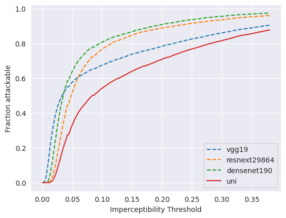
Figure 1: Fraction of attackable samples.

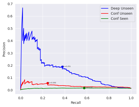
(a) Cifar10-robust

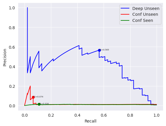
(b) Cifar100-robust

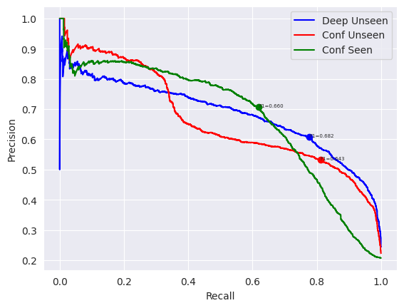
(c) Cifar10-att

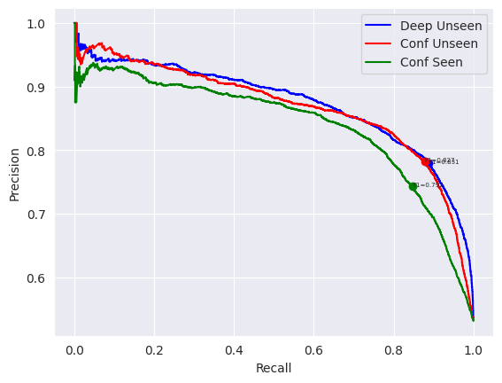
(d) Cifar100-att

Figure 2: P-R curves for detecting universal robust/attackable samples.

Section 5 describes a simple method to train a deep learning classifier to detect robust/attackable samples. Hence, a single layer fully connected network (Equation 9) is trained with seen (vgg, resnext, densenet) models’ encodings , using the validation samples in two binary classification settings: 1) detect attackable samples and 2) detect robust samples. The number of hidden layer nodes for each model’s FCN is set to the encoder output size. Training of the FCNs used a batch-size of 64, 200 epochs, a learning rate of 1e-3 (with a factor 10 drop at epochs 100 and 150), momentum of 0.9 and weight decay of 1e-4 with stochastic gradient descent. As described in Section 5 and inspired by Kim et al. (2021), an ensemble of the confidence of the three seen architectures, with no access to the target unseen architecture (conf-u) and the confidence of the target architecture, wrn, i.e. having seen the target architecture (conf-s) are also used as uncertainty based detectors for comparison to the deep-learning based (deep) attackability/robust sample detector. To better understand the operation of the detectors, Section 5 defines four evaluation settings: all (Equation 12), uni (Equation 13), spec (Equation 14) and vspec (Equation 15). Table 2 shows the F1 scores for detecting attackable samples on the unseen test data for the unseen wrn model, in the matched setting (FGSM attack used to define perturbation sizes for each sample in the test dataset). Note that the scale of F1 scores can vary significantly between evaluation settings as the prevalence of samples defined as attackable in a dataset are different for each setting. Table 3 presents the equivalent results for detecting robust samples, where the definitions for each evaluation setting update to identifying robust samples ($\mathbf{R}_{n,k}$). For Cifar10 data, the deep unseen detection method performs the best only in the uni evaluation setting for both attackable and robust sample detection. This is perhaps expected due to the deep detection method having been designed for this purpose (Equation 11), whilst for example the conf seen detection method has direct access to the target unseen model (wrn) and is able to perform better in the spec and vspec settings. When evaluation is on all attackable/robust samples for wrn, the superior vspec and spec performances of the uncertainty detectors, allows them to do better overall. However, for Cifar100 data, the deep detection method is able to perform significantly better in every setting other than the vspec evaluation setting, which is expected as this detector has no access to the target model and cannot identify samples specifically attackable/robust for the target model (wrn).

Setting		conf-s	conf-u	deep
all	cifar10	0.693	0.681	0.683
	cifar100	0.845	0.851	0.874
uni	cifar10	0.660	0.643	0.682
	cifar100	0.792	0.827	0.831
spec	cifar10	0.239	0.209	0.206
	cifar100	0.263	0.261	0.271
vspec	cifar10	0.010	0.006	0.006
	cifar100	0.018	0.018	0.018

Table 2: Attackable Sample Detection (F1) in matched setting.

Setting		conf-s	conf-u	deep
all	cifar10	0.501	0.502	0.435
	cifar100	0.134	0.161	0.385
uni	cifar10	0.030	0.090	0.251
	cifar100	0.026	0.074	0.565
spec	cifar10	0.486	0.485	0.422
	cifar100	0.119	0.141	0.286
vspec	cifar10	0.300	0.288	0.254
	cifar100	0.042	0.061	0.055

Table 3: Robust Sample Detection (F1) in matched setting.

Figure 2(a-b) presents the full precision-recall curves (as described in Section 5) for detecting robust samples in the uni evaluation setting, which the deep-learning based detector has been designed for. It is evident that for a large range of operating points, the deep detection method dominates and is thus truly a useful method for identifying robust samples. Figure 2(c-d) presents the equivalent precision-recall curves for detecting attackable samples. Here, although the deep-learning method still dominates over the uncertainty-based detectors, the differences are less significant. Hence, it can be argued that this deep learning-based attackability detector is capable of identifying both attackable and robust samples, but is particularly powerful in detecting robust samples.

In the unmatched evaluation setting the aim is to identify the attackable/robust samples in the test data, where the perturbation sizes for each sample are calculated using the more powerful unknown PGD attack method (Equation 4). PGD attacks used 8 iterations of the attack loop. For each model and dataset, the known FGSM attack and the unknown PGD attacks were used to rank samples in the validation set by the perturbation size, $|\boldsymbol{\delta}_{n}|$. In all cases the Spearman Rank correlation is greater than 0.84 for Cifar10 and 0.90 for Cifar100 (Table 4). This implies that the results from the matched setting should transfer easily to the unmatched setting.

	vgg	resnext	densenet
cifar10	0.840	0.849	0.951
cifar100	0.947	0.900	0.911

Table 4: Spearman rank correlation (PGD, FGSM) perturbations.

Table 5 gives the F1 scores for detecting universal attackable/robust samples in the unmatched setting. As the PGD attack is more powerful than the FGSM attack, the definition of the attackable threshold and robustness threshold are adjusted to $\epsilon_{a}=0.03$ and $\epsilon_{r}=0.10$. The deep unseen detectors dominate once again (specifically for robust sample detection) and thus, the trends identified for the matched evaluation setting are maintained in the more challenging unmatched setting.

Uni setting		conf-s	conf-u	deep
Attackable	cifar10	0.636	0.754	0.777
	cifar100	0.846	0.871	0.893
Robust	cifar10	0.008	0.008	0.048
	cifar100	0.005	0.006	0.233

Table 5: Attackable/Robust sample detection (unmatched setting).

7 Conclusion

This work proposes a novel perspective on adversarial attacks by formalizing the concept of sample attackability and robustness. A sample can be defined as attackable if its minimum perturbation size (for a successful adversarial attack) is less than a set threshold and conversely a sample can be defined as robust if its minimum perturbation size is greater than another set threshold. A deep-learning based attackability detector is trained to identify universally attackable/robust samples for unseen data and an unseen target model. In comparison to uncertainty-based attackability detectors, the deep-learning method performs best, with significant gains for robust sample detection. The understanding of sample attackability and robustness can have important implications for various tasks such as active adversarial training. Future work can explore the significance of attackability on the design of more robust systems.

Appendix A Unmatched Setting Detailed Results

Here more detailed results are presented for detecting attackable (Table 6) and robust samples (Table 7) in an unmatched setting, where the adversarial attack method used to measure the sample adversarial perturbation size (PGD) is different from the attack method (FGSM) available during training of the attackability detector. Recall that attackability is defined as the minimum perturbation size in Equation 5.

Setting		conf-s	conf-u	deep
all	cifar10	0.694	0.776	0.797
	cifar100	0.886	0.882	0.907
uni	cifar10	0.636	0.754	0.777
	cifar100	0.846	0.871	0.893
spec	cifar10	0.245	0.245	0.261
	cifar100	0.167	0.167	0.167
vspec	cifar10	0.012	0.012	0.012
	cifar100	0.006	0.006	0.006

Table 6: Attackable Sample Detection (F1) in unmatched setting.

Setting		conf-s	conf-u	deep
all	cifar10	0.195	0.291	0.146
	cifar100	0.088	0.114	0.307
uni	cifar10	0.008	0.008	0.048
	cifar100	0.005	0.006	0.233
spec	cifar10	0.192	0.288	0.144
	cifar100	0.084	0.113	0.277
vspec	cifar10	0.149	0.221	0.110
	cifar100	0.041	0.055	0.095

Table 7: Robust Sample Detection (F1) in unmatched setting.

Appendix B Extra Unseen Attack Method Experiments

Experiments in the main paper consider the unmatched setting where an attackability detector is trained using FGSM attacked sample perturbation sizes, but evaluated on samples with perturbation sizes defined using the unseen PGD attack method. This section considers further popular adversarial attack methods as unseen attack methods used to measure sample perturbation sizes. Specifically, we consider the Basic Iterative Method (BIM) (Kurakin et al., 2016), as an attack method with a similar algorithm to the PGD attack method. It is more interesting to understand how sample attackability (minimum perturbation size as per Equation 5) changes when the perturbation sizes are measured using attack methods very different attack algorithms. This may be of interest to a user when trying to understand which samples are susceptible to adversarial attacks in realistic settings, where an adversary may try a range of different attack approaches. Hence, we consider three common whitebox adversarial attack methods to define sample attackability: L-BFGS (Tabacof & Valle, 2015), C&W (Carlini & Wagner, 2016) and JSMA (Papernot et al., 2015).

Table 8 gives the Spearman Rank correlation for minimum perturbation sizes between samples for the FGSM (seen) and the selected (unseen) adversarial attack methods. It is clear that, as was the case with the PGD attack, for Cifar10 and Cifar100, FGSM and BIM attack approaches have a very strong perturbation size correlation. This is perhaps expected as both attack methods are not too dis-similar gradient-based approaches, so will give similar measures of sample attackability. However, the more different attack methods (JSMA, C&W and L-BFGS) have only a slightly lower rank correlation, suggesting that an attackability detector trained using a simple FGSM attack method can also transfer well in identifying the adversarially attackable and robust samples, where their attackability is defined using very different unseen attack methods.

Attack	Data	vgg	resnext	densenet
BIM	cifar10	0.871	0.866	0.950
	cifar100	0.946	0.914	0.921
C&W	cifar10	0.869	0.820	0. 945
	cifar100	0.928	0.919	0.910
L-BFGS	cifar10	0.845	0.825	0.938
	cifar100	0.936	0.907	0.928
JSMA	cifar10	0.838	0.852	0.901
	cifar100	0.922	0.899	0.912

Table 8: Spearman Rank Correlation between FGSM-based and other attack method based sample perturbation sizes (attackability).

Appendix C Active Adversarial Training

Adversarial training (Qian et al., 2022) is performed by further training trained models on adversarial examples, generated by adversarially attacking original data samples. However, it is computationally expensive to adversarially attack every original data sample. Hence, it is useful to actively select a subset of the most useful samples for adversarial training. Active adversarial training can be viewed as a strict form of weighted adversarial training (Holtz et al., 2022), where adversarial examples are re-weighed in importance during training. Figure 3 shows the robustness (measured by fooling rate)  of the target wide-resnet model when adversarially trained using adversarial examples from a subset of the Cifar10 validation data, where the subset is created by different ranking methods: 1) random; 2) a popular entropy-aware approach (Kim et al., 2021), where ranking is as per the uncertainty (entropy) of the trained wide-resent model (uncertainty); and 3) the final ranking method uses the attackability of original validation samples as per the deep attackability detector (unaware of the target wide-resnet model) from this work. The adversarially trained model’s robustness is evaluated using the fooling rate on the test Cifar10 data. It is evident that the deep attackability detector gives the most robust model for any fraction of data used for adversarial training. Specifically, with this detector, only 40% of the samples have to be adversarially attacked for adversarial training to give competitive robustness gains.

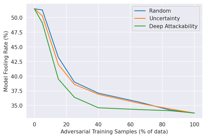
Figure 3: Active Adversarial Training

References

- Bai et al. (2021) Bai, T., Luo, J., Zhao, J., Wen, B., and Wang, Q. Recent advances in adversarial training for adversarial robustness. In Zhou, Z.-H. (ed.), Proceedings of the Thirtieth International Joint Conference on Artificial Intelligence, IJCAI-21, pp. 4312–4321. International Joint Conferences on Artificial Intelligence Organization, 8 2021. doi: 10.24963/ijcai.2021/591. URL https://doi.org/10.24963/ijcai.2021/591. Survey Track.
- Biggio & Roli (2017) Biggio, B. and Roli, F. Wild patterns: Ten years after the rise of adversarial machine learning. CoRR, abs/1712.03141, 2017. URL http://arxiv.org/abs/1712.03141.
- Carlini & Wagner (2016) Carlini, N. and Wagner, D. A. Towards evaluating the robustness of neural networks. CoRR, abs/1608.04644, 2016. URL http://arxiv.org/abs/1608.04644.
- Chakraborty et al. (2018) Chakraborty, A., Alam, M., Dey, V., Chattopadhyay, A., and Mukhopadhyay, D. Adversarial attacks and defences: A survey. CoRR, abs/1810.00069, 2018. URL http://arxiv.org/abs/1810.00069.
- Ducoffe & Precioso (2018) Ducoffe, M. and Precioso, F. Adversarial active learning for deep networks: a margin based approach. CoRR, abs/1802.09841, 2018. URL http://arxiv.org/abs/1802.09841.
- Gawlikowski et al. (2021) Gawlikowski, J., Tassi, C. R. N., Ali, M., Lee, J., Humt, M., Feng, J., Kruspe, A. M., Triebel, R., Jung, P., Roscher, R., Shahzad, M., Yang, W., Bamler, R., and Zhu, X. X. A survey of uncertainty in deep neural networks. CoRR, abs/2107.03342, 2021. URL https://arxiv.org/abs/2107.03342.
- Ghosh et al. (2018) Ghosh, P., Losalka, A., and Black, M. J. Resisting adversarial attacks using gaussian mixture variational autoencoders. CoRR, abs/1806.00081, 2018. URL http://arxiv.org/abs/1806.00081.
- Gilmer et al. (2018) Gilmer, J., Metz, L., Faghri, F., Schoenholz, S. S., Raghu, M., Wattenberg, M., and Goodfellow, I. J. Adversarial spheres. CoRR, abs/1801.02774, 2018. URL http://arxiv.org/abs/1801.02774.
- Goodfellow et al. (2014) Goodfellow, I. J., Shlens, J., and Szegedy, C. Explaining and harnessing adversarial examples, 2014. URL https://arxiv.org/abs/1412.6572.
- Gu & Rigazio (2014) Gu, S. and Rigazio, L. Towards deep neural network architectures robust to adversarial examples, 2014. URL https://arxiv.org/abs/1412.5068.
- He (2020) He, Z. Deep learning in image classification: A survey report. In 2020 2nd International Conference on Information Technology and Computer Application (ITCA), pp. 174–177, 2020. doi: 10.1109/ITCA52113.2020.00043.
- Hendrycks & Gimpel (2016) Hendrycks, D. and Gimpel, K. Visible progress on adversarial images and a new saliency map. CoRR, abs/1608.00530, 2016. URL http://arxiv.org/abs/1608.00530.
- Holtz et al. (2022) Holtz, C., Weng, T.-W., and Mishne, G. Learning sample reweighting for accuracy and adversarial robustness, 2022.
- Huynh et al. (2022) Huynh, N. D., Bouadjenek, M. R., Razzak, I., Lee, K., Arora, C., Hassani, A., and Zaslavsky, A. Adversarial attacks on speech recognition systems for mission-critical applications: A survey, 2022. URL https://arxiv.org/abs/2202.10594.
- Izmailov et al. (2018) Izmailov, R., Sugrim, S., Chadha, R., McDaniel, P., and Swami, A. Enablers of adversarial attacks in machine learning. In MILCOM 2018 - 2018 IEEE Military Communications Conference (MILCOM), pp. 425–430, 2018. doi: 10.1109/MILCOM.2018.8599715.
- Khurana et al. (2017) Khurana, D., Koli, A., Khatter, K., and Singh, S. Natural language processing: State of the art, current trends and challenges. CoRR, abs/1708.05148, 2017. URL http://arxiv.org/abs/1708.05148.
- Kim et al. (2021) Kim, M., Tack, J., Shin, J., and Hwang, S. J. Entropy weighted adversarial training. 2021.
- Krizhevsky (2009) Krizhevsky, A. Learning multiple layers of features from tiny images. pp. 32–33, 2009. URL https://www.cs.toronto.edu/~kriz/learning-features-2009-TR.pdf.
- Kurakin et al. (2016) Kurakin, A., Goodfellow, I. J., and Bengio, S. Adversarial machine learning at scale. CoRR, abs/1611.01236, 2016. URL http://arxiv.org/abs/1611.01236.
- Lee et al. (2017) Lee, H., Han, S., and Lee, J. Generative adversarial trainer: Defense to adversarial perturbations with GAN. CoRR, abs/1705.03387, 2017. URL http://arxiv.org/abs/1705.03387.
- Madry et al. (2017) Madry, A., Makelov, A., Schmidt, L., Tsipras, D., and Vladu, A. Towards deep learning models resistant to adversarial attacks, 2017. URL https://arxiv.org/abs/1706.06083.
- Meng & Chen (2017) Meng, D. and Chen, H. Magnet: a two-pronged defense against adversarial examples. CoRR, abs/1705.09064, 2017. URL http://arxiv.org/abs/1705.09064.
- Muhammad & Bae (2022) Muhammad, A. and Bae, S.-H. A survey on efficient methods for adversarial robustness. IEEE Access, 10:118815–118830, 2022. doi: 10.1109/ACCESS.2022.3216291.
- Papernot et al. (2015) Papernot, N., McDaniel, P. D., Jha, S., Fredrikson, M., Celik, Z. B., and Swami, A. The limitations of deep learning in adversarial settings. CoRR, abs/1511.07528, 2015. URL http://arxiv.org/abs/1511.07528.
- Qian et al. (2022) Qian, Z., Huang, K., Wang, Q.-F., and Zhang, X.-Y. A survey of robust adversarial training in pattern recognition: Fundamental, theory, and methodologies, 2022. URL https://arxiv.org/abs/2203.14046.
- Raina & Gales (2022) Raina, V. and Gales, M. Residue-based natural language adversarial attack detection. In Proceedings of the 2022 Conference of the North American Chapter of the Association for Computational Linguistics: Human Language Technologies. Association for Computational Linguistics, 2022. doi: 10.18653/v1/2022.naacl-main.281. URL https://doi.org/10.18653%2Fv1%2F2022.naacl-main.281.
- Ren et al. (2020) Ren, P., Xiao, Y., Chang, X., Huang, P., Li, Z., Chen, X., and Wang, X. A survey of deep active learning. CoRR, abs/2009.00236, 2020. URL https://arxiv.org/abs/2009.00236.
- Ru et al. (2020) Ru, D., Feng, J., Qiu, L., Zhou, H., Wang, M., Zhang, W., Yu, Y., and Li, L. Active sentence learning by adversarial uncertainty sampling in discrete space. In Findings of the Association for Computational Linguistics: EMNLP 2020, pp. 4908–4917, Online, November 2020. Association for Computational Linguistics. doi: 10.18653/v1/2020.findings-emnlp.441. URL https://aclanthology.org/2020.findings-emnlp.441.
- Sen et al. (2020) Sen, A., Zhu, X., Marshall, E., and Nowak, R. Popular imperceptibility measures in visual adversarial attacks are far from human perception. In Zhu, Q., Baras, J. S., Poovendran, R., and Chen, J. (eds.), Decision and Game Theory for Security, pp. 188–199, Cham, 2020. Springer International Publishing. ISBN 978-3-030-64793-3.
- Serban et al. (2020) Serban, A., Poll, E., and Visser, J. Adversarial examples on object recognition: A comprehensive survey. CoRR, abs/2008.04094, 2020. URL https://arxiv.org/abs/2008.04094.
- Shaham et al. (2018) Shaham, U., Garritano, J., Yamada, Y., Weinberger, E., Cloninger, A., Cheng, X., Stanton, K., and Kluger, Y. Defending against adversarial images using basis functions transformations, 2018. URL https://arxiv.org/abs/1803.10840.
- Shen et al. (2019) Shen, C., Peng, Y., Zhang, G., and Fan, J. Defending against adversarial attacks by suppressing the largest eigenvalue of fisher information matrix. CoRR, abs/1909.06137, 2019. URL http://arxiv.org/abs/1909.06137.
- Smith & Gal (2018) Smith, L. and Gal, Y. Understanding measures of uncertainty for adversarial example detection, 2018. URL https://arxiv.org/abs/1803.08533.
- Song et al. (2017) Song, Y., Kim, T., Nowozin, S., Ermon, S., and Kushman, N. Pixeldefend: Leveraging generative models to understand and defend against adversarial examples. CoRR, abs/1710.10766, 2017. URL http://arxiv.org/abs/1710.10766.
- Sun & Wang (2010) Sun, L.-L. and Wang, X.-Z. A survey on active learning strategy. In 2010 International Conference on Machine Learning and Cybernetics, volume 1, pp. 161–166, 2010. doi: 10.1109/ICMLC.2010.5581075.
- Szegedy et al. (2013) Szegedy, C., Zaremba, W., Sutskever, I., Bruna, J., Erhan, D., Goodfellow, I., and Fergus, R. Intriguing properties of neural networks, 2013. URL https://arxiv.org/abs/1312.6199.
- Tabacof & Valle (2015) Tabacof, P. and Valle, E. Exploring the space of adversarial images. CoRR, abs/1510.05328, 2015. URL http://arxiv.org/abs/1510.05328.
- Tanay & Griffin (2016) Tanay, T. and Griffin, L. D. A boundary tilting persepective on the phenomenon of adversarial examples. CoRR, abs/1608.07690, 2016. URL http://arxiv.org/abs/1608.07690.
- Xu et al. (2022) Xu, J., Zhang, C., Zheng, X., Li, L., Hsieh, C.-J., Chang, K.-W., and Huang, X. Towards adversarially robust text classifiers by learning to reweight clean examples. In Findings of the Association for Computational Linguistics: ACL 2022, pp. 1694–1707, Dublin, Ireland, May 2022. Association for Computational Linguistics. doi: 10.18653/v1/2022.findings-acl.134. URL https://aclanthology.org/2022.findings-acl.134.
- Zeng et al. (2020) Zeng, H., Zhu, C., Goldstein, T., and Huang, F. Are adversarial examples created equal? A learnable weighted minimax risk for robustness under non-uniform attacks. CoRR, abs/2010.12989, 2020. URL https://arxiv.org/abs/2010.12989.
- Zhang et al. (2019) Zhang, W. E., Sheng, Q. Z., and Alhazmi, A. Generating textual adversarial examples for deep learning models: A survey. CoRR, abs/1901.06796, 2019. URL http://arxiv.org/abs/1901.06796.