Extremal Domain Translation with Neural Optimal Transport

Abstract

In many unpaired image domain translation problems, e.g., style transfer or super-resolution, it is important to keep the translated image similar to its respective input image. We propose the extremal transport (ET) which is a mathematical formalization of the theoretically best possible unpaired translation between a pair of domains w.r.t. the given similarity function. Inspired by the recent advances in neural optimal transport (OT), we propose a scalable algorithm to approximate ET maps as a limit of partial OT maps. We test our algorithm on toy examples and on the unpaired image-to-image translation task. The code is publicly available at

https://github.com/milenagazdieva/ExtremalNeuralOptimalTransport

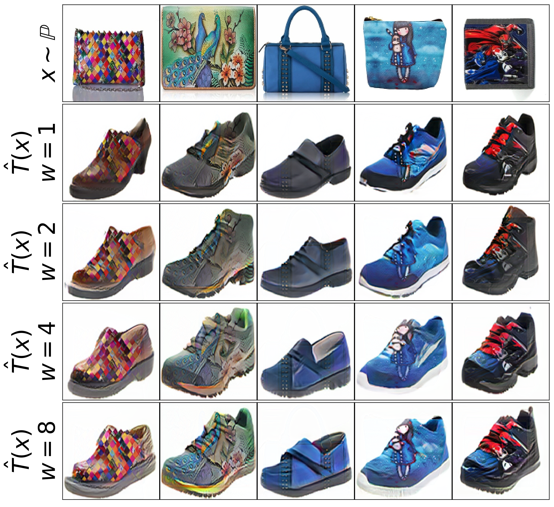
(a) Handbag $\rightarrow$ shoes (128$\times$128).

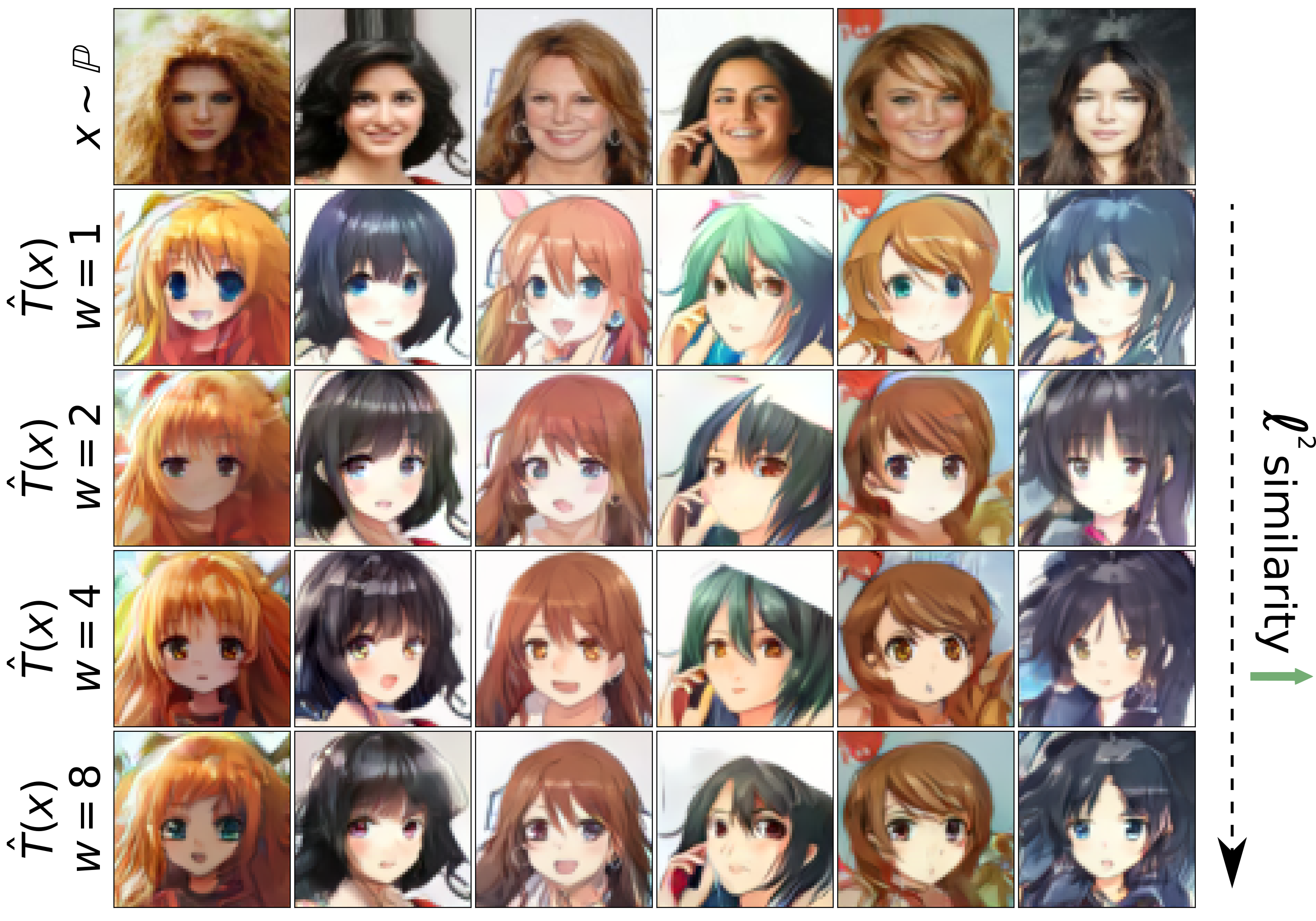
(b) Celeba (female) $\rightarrow$ anime (64$\times$64).

Figure 1: (Nearly) extremal transport with our Algorithm 1. Higher $w$ yields bigger similarity of $x$ and $T(x)$ in $\ell^{2}$.

1 Introduction

The unpaired translation task [72, Fig. 2] is to find a map $x\mapsto T(x)$, usually a neural network, which transports the samples $x$ from the given source domain to the target domain. The key challenge here is that the correspondence between available data samples $x$ from the source and $y$ from target domains is not given. Thus, the task is ambiguous as there might exist multiple suitable $T$.

Figure 2: Learned transport map ($w=2$) in ’Accept’ task.

When solving the task, many methods regularize the translated samples $T(x)$ to inherit specific attributes of the respective input samples $x$. In the popular unpaired translation [72, Fig. 9] and enhancement [69, Equation 3] tasks for images, it is common to use additional unsupervised identity losses, e.g., $\|T(x)-x\|_{1}$, to make the translated output $T(x)$ be similar to the input images $x$. The same applies, e.g., to audio translation [51]. Therefore, the learning objectives of such methods usually have two components. The first component is the domain loss (main) enforcing the translated sample $T(x)$ to look like the samples $y$ from the target domain. The second component is the similarity loss (regularizer, optional) stimulating the translated $T(x)$ to inherit certain attributes of input $x$. A question arises: can one obtain the maximal similarity of $T(x)$ to $x$ but still ensure that $T(x)$ is indeed from the target domain? A straightforward "yes, just increase the weight of the similarity loss" may work but only to a limited extent. We demonstrate this in Appendix C.

Contributions. In this paper, we propose the extremal transport (ET, 3.1) which is a rigorous mathematical task formulation describing the theoretically best possible unpaired domain translation w.r.t. the given similarity function. We explicitly characterize ET maps and plans by establishing an intuitive connection to the nearest neighbors (NN). We show that ET maps can be learned as a limit (3.3) of specific partial optimal transport (OT) problem which we call incomplete transport (IT, 3.2). For IT, we derive the duality formula yielding an efficient computational algorithm (3.4). We test our algorithm on toy 2D examples and high-dimensional unpaired image translation (5).

Notation. We consider compact Polish spaces ${(\mathcal{X},\|\!\cdot\!\|_{\mathcal{X}})}$, ${(\mathcal{Y},\|\!\cdot\!\|_{\mathcal{Y}})}$ and use $\mathcal{P}(\mathcal{X}),\mathcal{P}(\mathcal{Y})$ to denote the sets of Radon probability measures on them. We use $\mathcal{M}_{+}(\mathcal{X})\subset\mathcal{M}(\mathcal{X})$ to denote the sets of finite non-negative and finite signed (Radon) measures on $\mathcal{X}$, respectively. They both contain $\mathcal{P}(\mathcal{X})$ as a subset. For a non-negative $\mu\in\mathcal{M}_{+}(\mathcal{X})$, its support is denoted by $\text{Supp}(\mu)\subset\mathcal{X}$. It is a closed set consisting of all points $x\in\mathcal{X}$ for which every open neighbourhood $A\ni x$ satisfies $\mu(A)>0$. We use $\mathcal{C}(\mathcal{X})$ to denote the set of continuous functions $\mathcal{X}\rightarrow\mathbb{R}$ equipped with $\|\cdot\|_{\infty}$ norm. Its dual space is $\mathcal{M}(\mathcal{X})$ equipped with the $\|\cdot\|_{1}$ norm. A sequence $\mu_{1},\mu_{2},\dots\in\mathcal{M}(\mathcal{X})$ is said to be weakly-* converging to $\mu^{*}\in\mathcal{M}(\mathcal{X})$ if for every $f\in\mathcal{C}(\mathcal{X})$ it holds that $\lim_{n\rightarrow\infty}\int_{\mathcal{X}}f(x)d\mu_{n}(x)=\int_{\mathcal{X}}f(x)d\mu^{*}(x)$. For a probability measure $\pi\in\mathcal{P}(\mathcal{X}\times\mathcal{Y})$, we use $\pi_{x}\in\mathcal{P}(\mathcal{X})$ and $\pi_{y}\in\mathcal{P}(\mathcal{Y})$ to denote its projections onto $\mathcal{X},\mathcal{Y}$, respectively. Disintegration of $\pi$ yields $d\pi(x,y)=d\pi_{x}(x)d\pi(y|x)$, where $\pi(y|x)$ denotes the conditional distribution of $y\in\mathcal{Y}$ for a given $x\in\mathcal{X}$. For $\mu,\nu\in\mathcal{M}(\mathcal{Y})$, we write $\mu\leq\nu$ if for all measurable $A\subset\mathcal{Y}$ it holds that $\mu(A)\leq\nu(A)$. For a measurable map $T:\mathcal{X}\rightarrow\mathcal{Y}$, we use $T\sharp$ to denote the associated pushforward operator $\mathcal{P}(\mathcal{X})\rightarrow\mathcal{P}(\mathcal{Y})$.

2 Background on Optimal Transport

In this section, we give an overview of the OT theory concepts related to our paper. For details on OT, we refer to [62, 65, 56], partial OT - [22, 10].

Standard OT formulation. Let $c:\mathcal{X}\times\mathcal{Y}\rightarrow\mathbb{R}$ be a continuous cost function. For $\mathbb{P}\in\mathcal{P}(\mathcal{X})$, ${\mathbb{Q}\in\mathcal{P}(\mathcal{Y})}$, the OT cost between them is given by

$$\text{Cost}(\mathbb{P},\mathbb{Q})\stackrel{{\scriptstyle def}}{{=}}\inf_{T\sharp\mathbb{P}=\mathbb{Q}}\int_{\mathcal{X}}c\big{(}x,T(x)\big{)}d\mathbb{P}(x),$$ (1)

where $\inf$ is taken over measurable $T:\mathcal{X}\rightarrow\mathcal{Y}$ pushing $\mathbb{P}$ to $\mathbb{Q}$ (transport maps), see Fig. 3(a). Problem (1) is called the Monge’s OT problem, and its minimizer $T^{*}$ is called an OT map.

In some cases, there may be no minimizer $T^{*}$ of (1). Therefore, it is common to consider Kantorovich’s relaxation:

$$\text{Cost}(\mathbb{P},\mathbb{Q})\stackrel{{\scriptstyle def}}{{=}}\inf_{\pi\in\Pi(\mathbb{P},\mathbb{Q})}\int_{\mathcal{X}\times\mathcal{Y}}c(x,y)d\pi(x,y),$$ (2)

where $\inf$ is taken over $\pi\in\mathcal{P}(\mathcal{X}\times\mathcal{Y})$ satisfying $\pi_{x}=\mathbb{P}$ and $\pi_{y}=\mathbb{Q}$, respectively. A minimizer $\pi^{*}\in\Pi(\mathbb{P},\mathbb{Q})$ in (2) always exists and is called an OT plan. A widely used example of OT cost for $\mathcal{X}=\mathcal{Y}=\mathbb{R}^{d}$ is the Wasserstein-1 distance ($\mathbb{W}_{1}$), i.e., OT cost (2) for $c(x,y)=\|x-y\|$.

To provide an intuition behind (2), we disintegrate $d\pi(x,y)\!=\!d\pi_{x}(x)d\pi(y|x)$:

$$\inf_{\pi\in\Pi(\mathbb{P},\mathbb{Q})}\int_{\mathcal{X}}\bigg{\{}\int_{\mathcal{Y}}c(x,y)d\pi(y|x)\bigg{\}}\underbrace{d\mathbb{P}(x)}_{=d\pi_{x}(x)},$$ (3)

i.e., (2) can be viewed as an extension of (1) allowing to split the mass of input points $x\!\sim\!\mathbb{P}$ (Fig. 3(b)). With mild assumptions on $\mathbb{P},\mathbb{Q}$, the OT cost value (2) coincides with (1), see [62, Theorem 1.33].

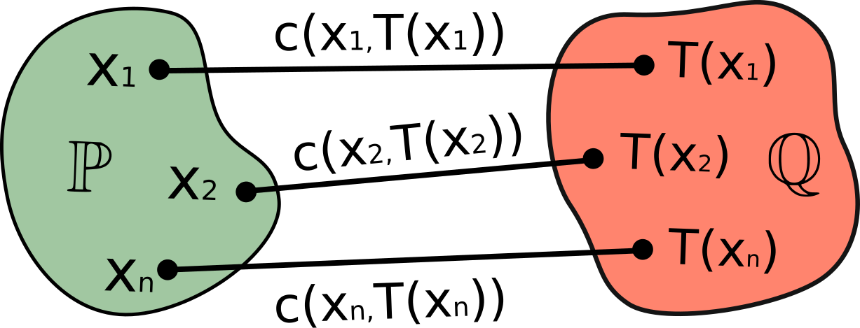
(a) Monge’s OT formulation.

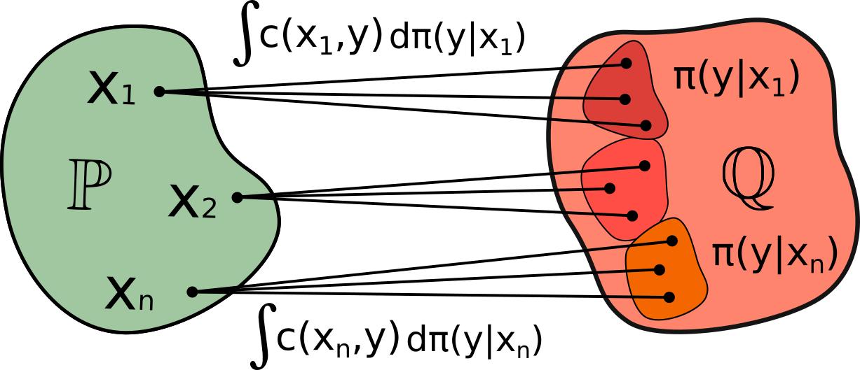
(b) Kantorovich’s OT formulation.

Figure 3: Classic optimal transport (OT) formulations.

 

Partial OT formulation. Let $w_{0},\!w_{1}\!\geq\!m\!\geq\!0$. We consider

$$\inf_{\begin{subarray}{c}m\pi_{x}\leq w_{0}\mathbb{P}\\ m\pi_{y}\leq w_{1}\mathbb{Q}\end{subarray}}\int_{\mathcal{X}\times\mathcal{Y}}c(x,y)d\big{[}m\pi\big{]}(x,y),$$ (4)

where $\inf$ is taken over $\pi\in\mathcal{P}(\mathcal{X}\times\mathcal{Y})$ satisfying the inequality constraints $m\pi_{x}\leq w_{0}\mathbb{P}$ and $m\pi_{y}\leq w_{1}\mathbb{Q}$. Minimizers $\pi^{*}$ of (4) are called partial OT plans (Fig. 4).

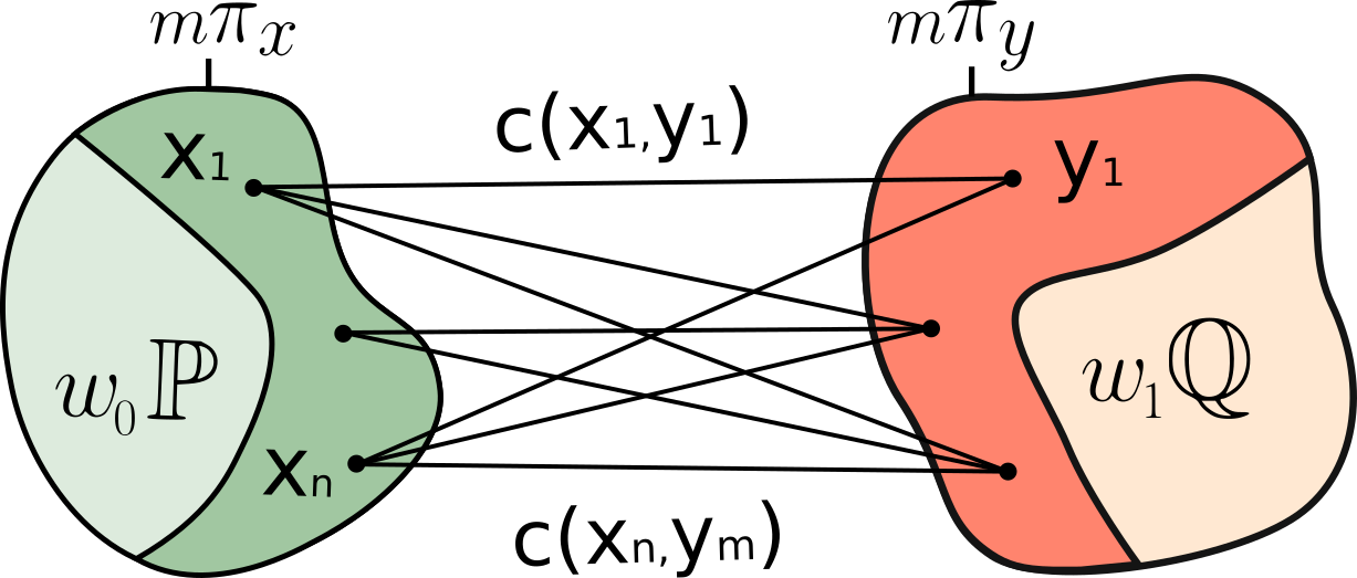
Figure 4: Partial optimal transport formulation.

Here the inputs are two measures $w_{0}\mathbb{P}$ and $w_{1}\mathbb{Q}$ with masses $w_{0}$ and $w_{1}$. Intuitively, we need to match a $\frac{m}{w_{0}}$-th fraction $m\pi_{x}$ of the first measure $w_{0}\mathbb{P}$ with a $\frac{m}{w_{1}}$-th fraction $m\pi_{y}$ of the second measure $w_{1}\mathbb{Q}$ (Fig. 4); choosing $\pi_{x},\pi_{y}$ is also a part of this problem. The key difference from problem (4) is that the constraints are inequalities. In the particular case $m=w_{0}=w_{1}$, problem (4) reduces to (2) as the inequality constraints can be replaced by equalities.

3 Main Results

First, we formulate the extremal transport (ET) problem (3.1). Next, we prove that ET maps can be recovered as a limit of incomplete transport (IT) maps (3.2, 3.3). Then we propose an algorithm to solve the IT problem (3.4). We provide the proofs for all the theorems in Appendix F.

3.1 Extremal Transport Problem

Popular unpaired translation methods, e.g., [72, 3.1] and [33, 3], de-facto assume that available samples $x,y$ from the input and output domains come from the data distributions $\mathbb{P},\mathbb{Q}\in\mathcal{P}(\mathcal{X}),\mathcal{P}(\mathcal{Y})$. As a result, in their optimization objectives, the domain loss compares the translated $T(x)\sim T\sharp\mathbb{P}$ and target samples $y\sim\mathbb{Q}$ by using a metric for comparing probability measures, e.g., GAN loss [27]. Thus, the target domain is identified with the probability measure $\mathbb{Q}$.

We pick a different approach to define what the domain is. We still assume that the available data comes from data distributions, i.e., $x\sim\mathbb{P},y\sim\mathbb{Q}$. However, we say that the target domain is the part of $\mathcal{Y}$ where the probability mass of $\mathbb{Q}$ lives. Namely, it is $\text{Supp}(\mathbb{Q})\subset\mathcal{Y}$. We say that a map $T$ translates the domains if $\text{Supp}(T\sharp\mathbb{P})\!\subset\!\text{Supp}(\mathbb{Q})$. This requirement is weaker than the usual $T\sharp\mathbb{P}\!=\!\mathbb{Q}$. Assume that $c(x,y)$ is a function estimating the dissimilarity between $x,y$. We would like to pick $T(x)\in\text{Supp}(\mathbb{Q})$ which is maximally similar to $x$ in terms of $c(x,y)$. This preference of $T$ can be formalized as follows:

$$\text{Cost}_{\infty}(\mathbb{P},\mathbb{Q})\stackrel{{\scriptstyle def}}{{=}}\inf_{\begin{subarray}{c}\text{Supp}(T\sharp\mathbb{P})\subset\text{Supp}(\mathbb{Q})\end{subarray}}\int_{\mathcal{X}}c\big{(}x,T(x)\big{)}d\mathbb{P}(x),$$ (5)

where the $\inf$ is taken over measurable ${T:\mathcal{X}\rightarrow\mathcal{Y}}$ which map the probability mass of $\mathbb{P}$ to $\text{Supp}(\mathbb{Q})$. We say that (5) is the (Monge’s) extremal transport (ET) problem.

Problem (5) is atypical for the common OT framework. For example, the usual measure-preserving constraint $T\sharp\mathbb{P}=\mathbb{Q}$ in (1) is replaced with $\text{Supp}(T\sharp\mathbb{P})\subset\text{Supp}(\mathbb{Q})$ which is more tricky. Importantly, measure $\mathbb{Q}$ can be replaced with any other ${\mathbb{Q}^{\prime}\in\mathcal{P}(\mathcal{Y})}$ with the same support yielding the same $\inf$. Below we analyse the minimizers $T^{*}$ of (5). We define $c^{*}(x)\stackrel{{\scriptstyle def}}{{=}}\min_{y\in\text{Supp}(\mathbb{Q})}c(x,y)$. Here the $\min$ is indeed attained (for all $x\in\mathcal{X}$) because $c(x,y)$ is continuous and $\text{Supp}(\mathbb{Q})\subset\mathcal{Y}$ is a compact set. The value $c^{*}(x)$ can be understood as the lowest possible transport cost when mapping the mass of point $x$ to the support of $\mathbb{Q}$. For any admissible $T$ in (5), it holds ($\mathbb{P}$-almost surely):

$$c^{*}(x)=\min_{y\in\text{Supp}(\mathbb{Q})}c(x,y)\leq c\big{(}x,T(x)\big{)}.$$ (6)

Proposition 1 (Continuity of $c^{*}$).

It holds that $c^{*}\in\mathcal{C}(\mathcal{X})$.

As a consequence of Proposition 1, we see that $c^{*}$ is measurable. We integrate (6) w.r.t. $x\sim\mathbb{P}$ and take $\inf$ over all feasible $T$. This yields a lower bound on $\text{Cost}_{\infty}(\mathbb{P},\mathbb{Q})$:

$$\int_{\mathcal{X}}c^{*}(x)d\mathbb{P}(x)\leq\overbrace{\inf_{\begin{subarray}{c}\text{Supp}(T\sharp\mathbb{P})\\ \subset\text{Supp}(\mathbb{Q})\end{subarray}}\int_{\mathcal{X}}c\big{(}x,T(x)\big{)}d\mathbb{P}(x)}^{\text{Cost}_{\infty}(\mathbb{P},\mathbb{Q})}.$$ (7)

There exists admissible $T$ making (7) the equality. Indeed, let $\text{NN}(x)\stackrel{{\scriptstyle def}}{{=}}\{y\in\text{Supp}(\mathbb{Q})$ s.t. $c(x,y)=c^{*}(x)\}$ be the set of points $y$ which attain $\min$ in the definition of $c^{*}$. These points are the closest to $x$ points in $\mathbb{Q}$ w.r.t. the cost $c(x,y)$. We call them the nearest neighbors of $x$. From this perspective, we see that (7) turns to equality if and only if $T(x)\!\in\!\text{NN}(x)$ holds for $\mathbb{P}$-almost all $x\in\mathcal{X}$, i.e., $T$ maps points $x\!\sim\!\mathbb{P}$ to their nearest neighbors in $\text{Supp}(\mathbb{Q})$. We need to make sure that such measurable $T$ exists (Fig. 5(a)).

Theorem 1 (Existence of ET maps).

There exists at least one measurable map $T^{*}:\mathcal{X}\rightarrow\mathcal{Y}$ minimizing (5). For $\mathbb{P}$-almost all $x\in\mathcal{X}$ it holds that $T^{*}(x)\in\text{NN}(x)$. Besides,

$$\text{Cost}_{\infty}(\mathbb{P},\mathbb{Q})=\int_{\mathcal{X}}c^{*}(x)d\mathbb{P}(x).$$

We say that $\text{Cost}_{\infty}(\mathbb{P},\mathbb{Q})$ is the extremal cost because one can not obtain smaller cost when moving the mass of $\mathbb{P}$ to $\text{Supp}(\mathbb{Q})$. In turn, we say that minimizers $T^{*}$ are ET maps.

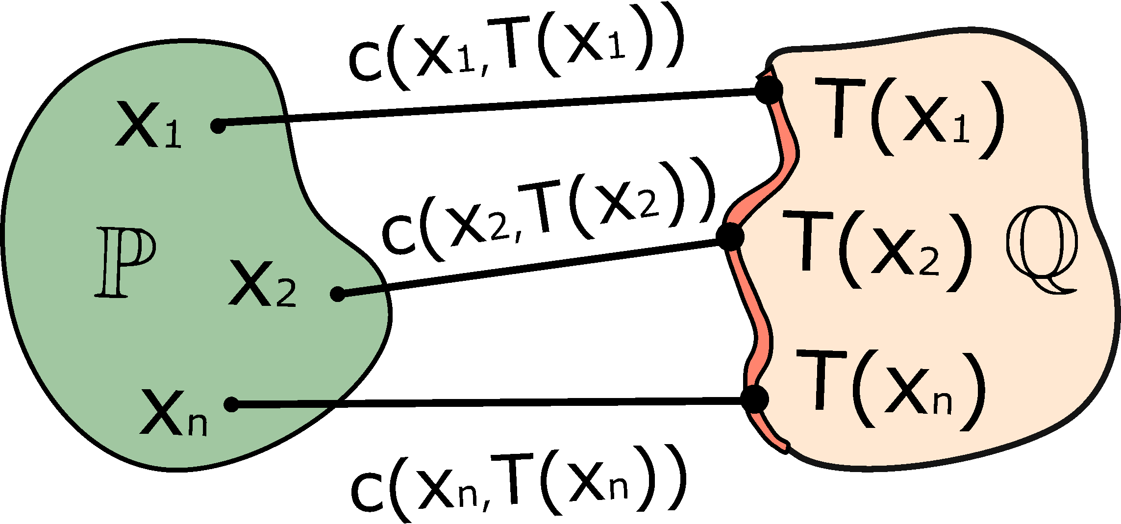
(a) Monge’s ET formulation.

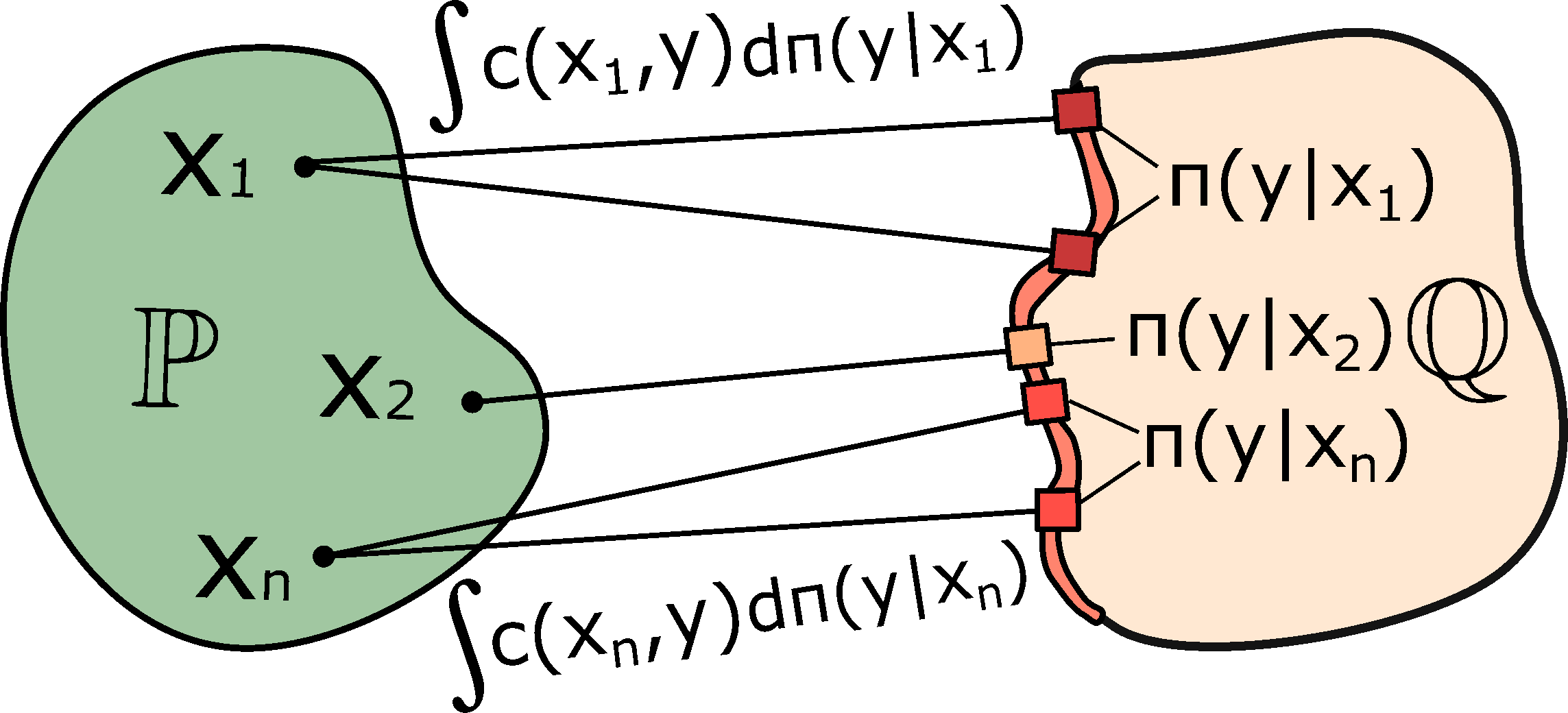
(b) Kantorovich’s ET formulation.

Figure 5: Extremal transport (ET) formulations.

 

One may extend the ET problem (8) in the Kantorovich’s manner by allowing the mass splitting and stochastic plans:

$$\text{Cost}_{\infty}(\mathbb{P},\mathbb{Q})\stackrel{{\scriptstyle def}}{{=}}\inf_{\pi\in\Pi^{\infty}(\mathbb{P},\mathbb{Q})}\int_{\mathcal{X}\times\mathcal{Y}}c(x,y)d\pi(x,y),$$ (8)

where $\Pi^{\infty}(\mathbb{P},\mathbb{Q})$ are probability measures $\pi\in\mathcal{P}(\mathcal{X}\times\mathcal{Y})$ s.t. $\pi_{x}=\mathbb{P}$ and $\text{Supp}(\pi_{y})\subset\text{Supp}(\mathbb{Q})$. To understand the structure of minimizers in (8), it is more convenient to disintegrate $d\pi(x,y)=d\pi(y|x)d\pi_{x}(x)$:

$$\text{Cost}_{\infty}(\mathbb{P},\mathbb{Q})=\inf_{\pi\in\Pi^{\infty}(\mathbb{P},\mathbb{Q})}\!\int_{\mathcal{X}}\!\int_{\mathcal{Y}}\!\!c(x,y)d\pi(y|x)\!\underbrace{d\mathbb{P}(x)}_{=d\pi_{x}(x)}\!.$$ (9)

Thus, computing (8) boils down to computing a family of conditional measures $\pi(\cdot|x)$ minimizing (8). As in (7), for any $\pi\in\Pi^{\infty}(\mathbb{P},\mathbb{Q})$, it holds (for $\mathbb{P}$-almost all $x\in\mathcal{X}$) that

$$c^{*}(x)=\min_{y\in\text{Supp}(\mathbb{Q})}c(x,y)\leq\int_{\mathcal{Y}}c(x,y)d\pi(y|x)$$ (10)

because $\pi$ redistributes the mass of $\mathbb{P}$ to $\text{Supp}(\mathbb{Q})$. By integrating (10) w.r.t. $x\sim\mathbb{P}=\pi_{x}$ and taking $\inf$ over all admissible plans $\pi$, we derive that $\int_{\mathcal{X}}c^{*}(x)d\mathbb{P}(x)$ is a lower bound for (8). In particular, the bound is tight for $\pi^{*}(y|x)=\delta_{T^{*}(x)}$, where $T^{*}$ is the ET map from our Theorem 1. Therefore, the value (8) is the same as (5) but possibly admits more minimizers. We call the minimizers $\pi^{*}$ of (8) the ET plans (Fig. 5(b)).

From (10) and the definition of $\text{NN}(x)$, we see that minimizers $\pi^{*}$ are the plans for which $\pi^{*}(y|x)$ redistributes the mass of $x$ among the nearest neighbors $y\in\text{NN}(x)$ of $x$ (for $\mathbb{P}$-almost all $x\in\mathcal{X}$). As a result, $\pi^{*}(y|x)$ can be viewed as a stochastic nearest neighbor assignment between the probability mass of $\mathbb{P}$ and the support of $\mathbb{Q}$.

3.2 Incomplete Transport Problem

In practice, solving extremal problem (5) is challenging because it is hard to enforce $\text{Supp}(T\sharp\mathbb{P})\subset\text{Supp}(\mathbb{Q})$. To avoid enforcing this constraint, we replace it and consider the following problem with finite parameter $w\geq 1$:

$$\text{Cost}_{w}(\mathbb{P},\mathbb{Q})\stackrel{{\scriptstyle def}}{{=}}\inf_{T\sharp\mathbb{P}\leq w\mathbb{Q}}\int_{\mathcal{X}}c\big{(}x,T(x)\big{)}d\mathbb{P}(x).$$ (11)

We call (11) Monge’s incomplete transport (IT) problem (Fig. 6(a)). With the increase of $w$, admissible maps $T$ obtain more ways to redistribute the mass of $\mathbb{P}$ among $\text{Supp}(\mathbb{Q})$. Informally, when $w\rightarrow\infty$, the constraint $T\sharp\mathbb{P}\leq w\mathbb{Q}$ in (11) tends to the constraint $\text{Supp}(T\sharp\mathbb{P})\subset\text{Supp}(\mathbb{Q})$ in (5), i.e., (11) itself tends to ET problem (5). We will formalize this statement a few paragraphs later (in 3.3).

As in (1), problem (11) may have no minimizer $T^{*}$ or even may have the empty feasible set. Therefore, it is natural to relax problem (11) in the Kantorovich’s manner:

$$\text{Cost}_{w}(\mathbb{P},\mathbb{Q})\stackrel{{\scriptstyle def}}{{=}}\inf_{\pi\in\Pi^{w}(\mathbb{P},\mathbb{Q})}\int_{\mathcal{X}\times\mathcal{Y}}c(x,y)d\pi(x,y),$$ (12)

where the $\inf$ is taken over the set $\Pi^{w}(\mathbb{P},\mathbb{Q})$ of probability measures $\pi\in\mathcal{P}(\mathcal{X}\times\mathcal{Y})$ whose first marginal is $\pi_{x}=\mathbb{P}$, and the second marginal satisfies $\pi_{y}\leq w\mathbb{Q}$ (Fig. 6(b)).

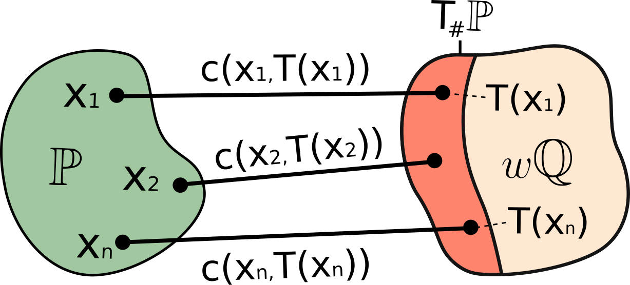
(a) Monge’s IT formulation.

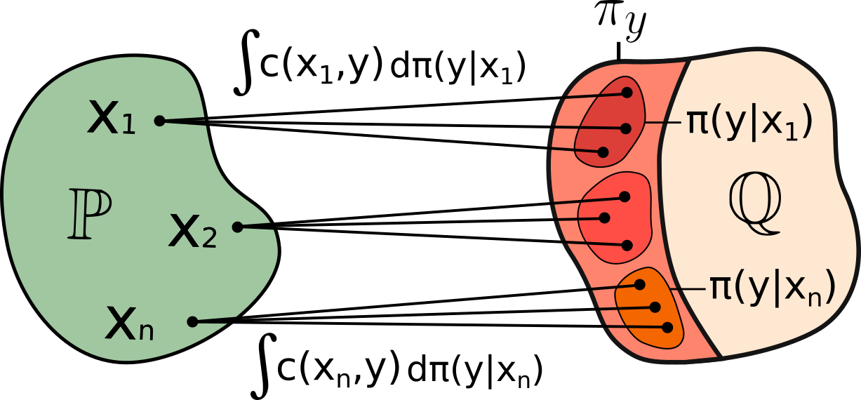
(b) Kantorovich’s IT formulation.

Figure 6: Incomplete transport (IT) formulations.

 

We note that IT problem (12) is a special case of partial OT (4) with $w_{0}=m=1$ and $w_{1}=w$. In (12), one may actually replace $\inf$ with $\min$, see our proposition below.

Proposition 2 (Existence of IT plans).

Problem (12) admits at least one minimizer $\pi^{*}\in\Pi^{w}(\mathbb{P},\mathbb{Q})$.

We say that minimizers of (12) are IT plans. In the general case, Kantorovich’s IT cost (12) always lower bounds Monge’s counterpart (11). Below we show that they coincide in the practically most interesting Euclidean case.

Proposition 3 (Equivalence of Monge’s, Kantorovich’s IT costs).

Let $\mathcal{X},\mathcal{Y}\subset\mathbb{R}^{D}$ be two compact sets, $\mathbb{P}\in\mathcal{P}(\mathcal{X})$ be atomless, $\mathbb{Q}\!\in\!\mathcal{P}(\mathcal{Y})$. Then Monge’s (11) and Kantorovich’s (12) IT costs coincide.

However, it is not guaranteed that $\inf$ in Monge’s problem (11) is attained even in the Euclidean case. Still for general Polish spaces $\mathcal{X},\mathcal{Y}$ it is clear that if there exists a deterministic IT plan in Kantorovich’s problem (12) of the form $\pi^{*}=[\text{id}_{\mathcal{X}},T^{*}]$, then $T^{*}$ is an IT map in (11), and the IT Monge’s (11) and Kantorovich’s (12) costs coincide. Henceforth, for simplicity, we assume that $\mathcal{X},\mathcal{Y},c,\mathbb{P},\mathbb{Q}$ are such that (11) and (12) coincide, e.g., those from Prop. 3.

IT problem (12) can be viewed as an interpolation between OT (2) and ET problems (8). Indeed, when $w=1$, the constraint $\pi_{y}\leq\mathbb{Q}$ is equivalent to $\pi_{y}=\mathbb{Q}$ as there is only one probability measure which is $\leq\mathbb{Q}$, and it is $\mathbb{Q}$ itself. Thus, IT (12) with $w=1$ coincides with OT (2). In the next section, we show that for $w\rightarrow\infty$ one recovers ET from IT.

3.3 Link between Incomplete and Extremal Transport

Now we connect incomplete (12) and extremal (8) transport tasks.

Theorem 2 (IT costs converge to the ET cost when ${w\rightarrow\infty}$).

Function $w\mapsto\text{Cost}_{w}(\mathbb{P},\mathbb{Q})$ is convex, non-increasing in $w\in[1,+\infty)$ and

$$\lim_{w\rightarrow\infty}\text{Cost}_{w}(\mathbb{P},\mathbb{Q})=\text{Cost}_{\infty}(\mathbb{P},\mathbb{Q}).$$

A natural subsequent question here is whether IT plans in (12) converge to ET plans (8) when $w\rightarrow\infty$. Our following result sheds the light on this question.

Theorem 3 (IT plans converge to ET plans when ${w\rightarrow\infty}$).

Consider $w_{1},w_{2},w_{3},\dots\geq 1$ satisfying ${\lim_{n\rightarrow\infty}w_{n}=\infty}$. Let $\pi^{w_{n}}\in\Pi^{w_{n}}(\mathbb{P},\mathbb{Q})$ be a sequence of IT plans solving (12) with $w=w_{n}$, respectively. Then it has a (weakly-*) converging sub-sequence. Every such sub-sequence of IT plans converges to an ET plan $\pi^{*}\in\Pi^{\infty}(\mathbb{P},\mathbb{Q})$.

In general, there may be sub-sequences of IT plans converging to different ET plans $\pi^{*}\in\Pi^{\infty}(\mathbb{P},\mathbb{Q})$. However, our following corollary shows that with the increase of weight $w$, elements of any sub-sequence become closer to the set of ET plans.

Corollary 1 (IT plans become closer to the set of ET plans when ${w\rightarrow\infty}$).

For all $\varepsilon>0$ $\exists w(\varepsilon)\in[1,\infty)$ such that $\forall w\geq w(\varepsilon)$ and $\forall$ IT plan $\pi^{w}\in\Pi_{w}(\mathbb{P},\mathbb{Q})$ solving Kantorovich’s IT problem (12), there exists an ET plan $\pi^{*}$ which is $\varepsilon$-close to $\pi^{w}$ in $\mathbb{W}_{1}$, i.e., $\mathbb{W}_{1}(\pi^{*},\pi^{w})\leq\varepsilon$.

Providing a stronger convergence result here is challenging, and we leave this theoretical question open for future studies. Our Theorems 2, 3 and Corollary 1 suggest that to obtain a fine approximation of an ET plan ($w=\infty$), one may use an IT plan for sufficiently large finite $w$. In Appendix G.1, we empirically demonstrate this observation through an experiment where the ground-truth deterministic ET plan is analytically known. Below we develop a neural algorithm to compute IT plans.

3.4 Computational Algorithm for Incomplete Transport

To begin with, for IT (12), we derive the dual problem.

Theorem 4 (Dual problem for IT).

It holds

$$\text{Cost}_{w}(\mathbb{P},\mathbb{Q})\!=\!\max_{f\leq 0}\!\int_{\mathcal{X}}f^{c}(x)d\mathbb{P}(x)\!+w\!\!\int_{\mathcal{Y}}\!f(y)d\mathbb{Q}(y),$$ (13)

where the $\max$ is taken over non-positive $f\in\mathcal{C}(\mathcal{Y})$ and $f^{c}(x)\stackrel{{\scriptstyle def}}{{=}}\min\limits_{y\in\mathcal{Y}}\big{\{}c(x,y)-f(y)\big{\}}$.

We call the function $f$ potential. In the definition of $f^{c}$, $\min$ is attained because $c,f$ are continuous and $\mathcal{Y}$ is compact. The function $f^{c}$ is called the $c$-transform of $f$.

The difference of formula (13) from usual $c$-transform-based duality formulas for OT (2), see [62, 1.2], [65, 5], is that $f$ is required to be non-positive and the second term is multiplied by $w\geq 1$. We rewrite the term $\int_{\mathcal{X}}f^{c}(x)d\mathbb{P}(x)$ in (13):

$$\int_{\mathcal{X}}f^{c}(x)d\mathbb{P}(x)=\int_{\mathcal{X}}\min\limits_{y\in\mathcal{Y}}\big{\{}c(x,y)-f(y)\big{\}}d\mathbb{P}(x)=\inf\limits_{T:\mathcal{X}\rightarrow\mathcal{Y}}\int_{\mathcal{X}}\big{\{}c\big{(}x,T(x)\big{)}-f(y)\big{\}}d\mathbb{P}(x).$$ (14)

Here we use the interchange between the integral and $\inf$ [59, Theorem 3A]; in (14) the $\inf$ is taken over measurable maps. Since $(x,y)\mapsto c(x,y)-f(y)$ is a continuous function on a compact set, it admits a measurable selection $T(x)\in\operatorname*{arg\,min}_{y\in\mathcal{Y}}\big{\{}c(x,y)-f(y)\big{\}}$ minimizing (14), see [2, Theorem 18.19]. Thus, $\inf$ can be replaced by $\min$. We combine (14) and (13) and obtain an equivalent saddle point problem:

$$\text{Cost}_{w}(\mathbb{P},\mathbb{Q})=\max_{f\leq 0}\min_{T:\mathcal{X}\rightarrow\mathcal{Y}}\mathcal{L}(f,T),$$ (15)

where the functional $\mathcal{L}(f,T)$ is defined by

$$\mathcal{L}(f,T)\stackrel{{\scriptstyle def}}{{=}}\int_{\mathcal{X}}c\big{(}x,T(x)\big{)}d\mathbb{P}(x)-\int_{\mathcal{X}}f\big{(}T(x)\big{)}d\mathbb{P}(x)+w\int_{\mathcal{Y}}f(y)d\mathbb{Q}(y).$$ (16)

Functional $\mathcal{L}(f,T)$ can be viewed as a Lagrangian with $f\leq 0$ being a multiplier for the constraint ${T\sharp\mathbb{P}-w\mathbb{Q}\leq 0}$. By solving (15), one may obtain IT maps.

Input : distributions $\mathbb{P},\mathbb{Q}$ accessible by samples; mapper $T_{\theta}\!:\!\mathcal{X}\!\rightarrow\!\mathcal{Y}$; potential $f_{\psi}:\!\mathcal{X}\!\rightarrow\!\mathbb{R}_{-}$;

transport cost $c:\mathcal{X}\times\mathcal{Y}\rightarrow\mathbb{R}$; weight $w\geq 1$; number $K_{T}$ of inner iterations;

Output : approximate IT map $(T_{\theta})_{\#}\mathbb{P}\leq w\mathbb{Q}$;

repeat

     Sample batches $X\sim\mathbb{P}$, $Y\!\sim\!\mathbb{Q}$;

     $\mathcal{L}_{f}\leftarrow w\cdot\frac{1}{|Y|}\sum\limits_{y\in Y}f_{\psi}(y)-\frac{1}{|X|}\sum\limits_{x\in X}f_{\psi}\big{(}T_{\theta}(x)\big{)}$;

     Update $\psi$ by using $\frac{\partial\mathcal{L}_{f}}{\partial\psi}$ to maximize $\mathcal{L}_{f}$;

    

    for $k_{T}=1,2,\dots,K_{T}$ do

         Sample batch $X\sim\mathbb{P}$;

         ${\mathcal{L}_{T}\leftarrow\frac{1}{|X|}\sum\limits_{x\in X}\big{[}c\big{(}x,T_{\theta}(x)\big{)}-f_{\psi}\big{(}T_{\theta}(x)\big{)}\big{]}}$;

         Update $\theta$ by using $\frac{\partial\mathcal{L}_{T}}{\partial\theta}$ to minimize $\mathcal{L}_{T}$;

        

    

until not converged;

Algorithm 1 Procedure to compute the IT map between $\mathbb{P}$ and $\mathbb{Q}$ for transport cost $c(x,y)$ and weight $w$.

Theorem 5 (IT maps are contained in optimal saddle points).

Let $f^{*}$ be any maximizer in (13). If $\pi^{*}\in\Pi^{w}(\mathbb{P},\mathbb{Q})$ is a deterministic IT plan, i.e., it solves (12) and has the form $\pi^{*}=[\text{id}_{\mathcal{X}},T^{*}]\sharp\mathbb{P}$ for some measurable ${T^{*}:\mathcal{X}\rightarrow\mathcal{Y}}$, then

$$T^{*}\in\operatorname*{arg\,min}_{T:\mathcal{X}\rightarrow\mathcal{Y}}\mathcal{L}(f^{*},T).$$

Our Theorem 5 states that in some optimal saddle points $(f^{*},T^{*})$ of (15) it holds that $T^{*}$ is the IT map between $\mathbb{P},\mathbb{Q}$. In general, the $\operatorname*{arg\,inf}_{T}$ set for an optimal $f^{*}$ might contain not only IT maps $T^{*}$, but other functions as well (fake solutions), see limitations in Appendix A.

We solve the optimization problem (15) by approximating the map $T$ and potential $f$ with neural networks $T_{\theta}$ and $f_{\psi}$, respectively. To make $f_{\psi}$ non-positive, we use ${x\mapsto-|x|}$ as the last layer. The nets are trained using random batches from $\mathbb{P},\mathbb{Q}$ and stochastic gradient ascent-descent. We detail the optimization procedure in Algorithm 1.

4 Related work

OT in generative models. A popular way to apply OT in generative models is to use the OT cost as the loss function to update the generator [4, 28, 26], see [41] for a survey. These methods are not relevant to our study as they do not learn an OT map but only compute the OT cost.

Recent works [43, 42, 61, 20, 5, 24, 29] are the most related to our study. These papers show the possibility to learn the OT maps (or plans) via solving saddle point optimization problems derived from the standard $c$-transform-based duality formulas for OT. The underlying principle of our objective (15) is analogous to theirs. The key difference is that they consider OT problems (1), (2) and enforce the equality costraints, e.g., $T\sharp\mathbb{P}=\mathbb{Q}$, while our approach enforces the inequality constraint $T\sharp\mathbb{P}\leq w\mathbb{Q}$ allowing to partially align the measures. We provide a detailed discussion of relation with these works as well as with the fundamental OT (2) and partial OT (4) literature [22, 10, 62] in Appendix F, see bibliographic remarks after the proofs of Theorems 2, 4 and 5.

For completeness, we also mention other existing neural OT methods [25, 63, 49, 17, 39]. These works are less related to our work because they either underperform compared to the above-mentioned saddle point methods, see [40] for evaluation, or they solve specific OT formulations, e.g., entropic OT [56, 4], which are not relevant to our study.

The papers [66, 47, 19] are slightly more related to our work. They propose neural methods for unbalanced OT [14] which can also be used to partially align measures. As we will see in Appendix B, UOT is hardly suitable for ET (8) as it is not easy to control how it spreads the probability mass. Besides, these methods consider OT between small-dimensional datasets or in latent spaces. It is not clear whether they scale to high-dimensions, e.g., images.

Discrete OT methods, including partial OT [11], are not relevant to us, see Appendix D for details.

Unpaired domain translation [3] is a generic problem which includes image super-resolution [12], inpainting [71], style translation [34] tasks, etc. Hence, we do not mention all of the existing approaches but focus on their common main features instead. In many applications, it is important to preserve semantic information during the translation, e.g., the image content. In most cases, to do this it is sufficient to use convolutional neural networks. They preserve the image content thanks to their design which is targeted to only locally change the image [18]. However, in some of the tasks additional image properties must be kept, e.g., image colors in super-resolution. Typical approaches to such problems are based on GANs and use additional similarity losses, e.g., the basic CycleGAN [72] enforces $\ell^{1}$ similarity. Such methods are mostly related to our work. However, without additional modifications most of these approaches only partially maintain the image properties, see [44, Figure 5]. As we show in experiments (Appendix C), IT achieves better similarity than popular CycleGAN, StarGAN-v2 [15] methods, both default and modified to better preserve the image content.

5 Evaluation

In 5.1, we provide illustrative toy 2D examples. In 5.2, we evaluate our method on the unpaired image-to-image translation task. Technical training details (architectures, learning rates, etc.) are given in Appendix E. The code is written using PyTorch framework and is publicly available at

https://github.com/milenagazdieva/ExtremalNeuralOptimalTransport.

Transport costs. We experiment with the quadratic cost $c(x,y)\!=\!\ell^{2}(x,y)$ as this cost already provides reasonable performance. We slightly abuse the notation and use $\ell^{2}$ to denote the squared error normalized by the dimension. Experiments with the perceptual cost are given in Appendix G.3.

5.1 Toy 2D experiments

In this section, we provide ’Wi-Fi’ and ’Accept’ examples in 2D to show how the choice of $w$ affects the fraction of the target measure $\mathbb{Q}$ to which the probability mass of the input $\mathbb{P}$ is mapped. In both cases, measure $\mathbb{P}$ is Gaussian. In Appendix B, we demonstrate how other methods perform on these ’Wi-Fi’ and ’Accept’ toy examples.

In ’Wi-Fi’ experiment (Fig. 7), target $\mathbb{Q}$ contains 3 arcs. We provide the learned IT maps for $w\in[1,\frac{3}{2},3]$. The results show that by varying $w$ it is possible to control the fraction of $\mathbb{Q}$ to which the mass of $\mathbb{P}$ will be mapped. In Fig. 7, we see that for $w=1$ our IT method learns all 3 arcs. For $w=\frac{3}{2}$, it captures 2 arcs, i.e., $\approx\frac{2}{3}$ of $\mathbb{Q}$. For $w=3$, it learns 1 arc which corresponds to $\approx\frac{1}{3}$ of $\mathbb{Q}$.

In ’Accept’ experiment (Fig. 2), target $\mathbb{Q}$ is a two-line text. Here we put $w=2$ and, as expected, our method captures only one line of the text which is the closest to $\mathbb{P}$ in $\ell^{2}$.

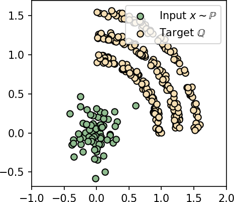
(a) Input, target measures.

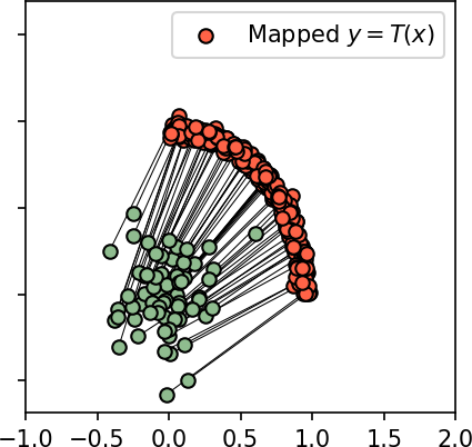
(b) IT map, $w\!=\!3$.

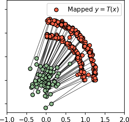
(c) IT map, $w\!=\!\frac{3}{2}$.

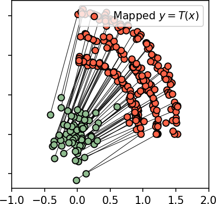
(d) IT map, $w\!=\!1$.

Figure 7: Incomplete transport (IT) maps learned by our Algorithm 1 in ’Wi-Fi’ experiment.

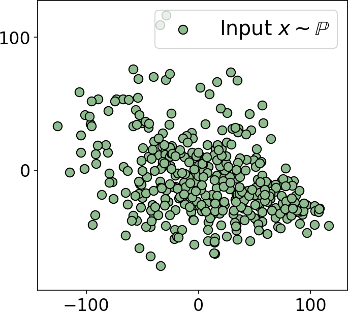
(a) Input measure.

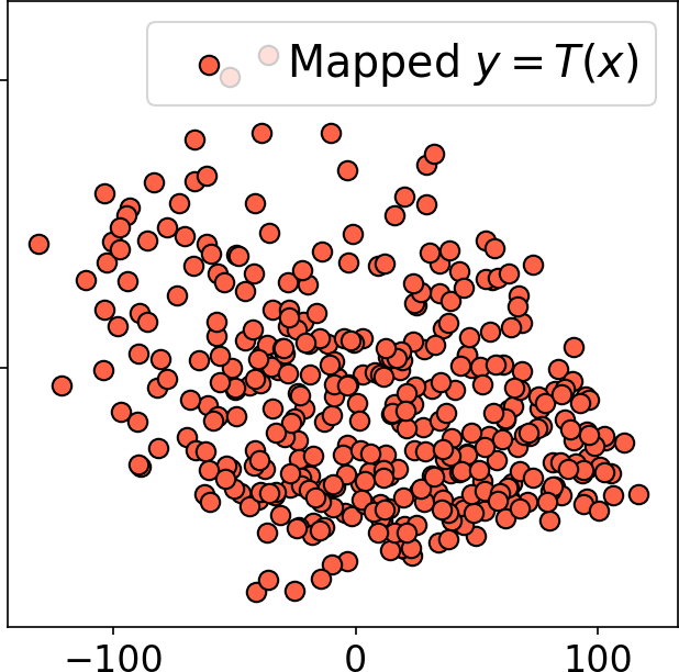
(b) IT map, $w\!=\!8$.

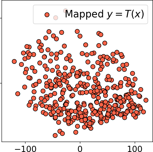
(c) IT map, $w\!=\!4$.

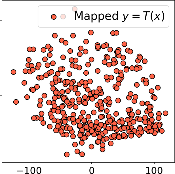
(d) IT map, $w\!=\!2$.

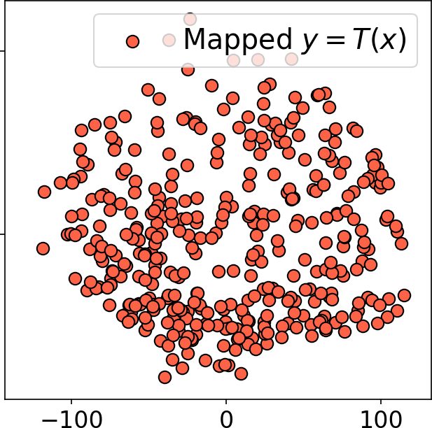
(e) IT map, $w\!=\!1$.

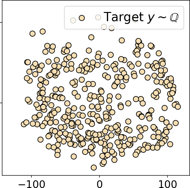
(f) Target measure.

Figure 8: PCA projections of input $x\!\sim\!\mathbb{P}$, mapped $T(x)\!\sim\!T\sharp\mathbb{P}$ and target $y\!\sim\!\mathbb{Q}$ test samples (handbag$\rightarrow$shoes experiment).

5.2 Unpaired Image-to-image Translation

Here we learn IT maps between various pairs of datasets. We test $w\!\in\!\{1,2,4,8\}$ in all experiments. For completeness, we consider bigger weights $w\in\{16,32\}$ in Appendix G.4.

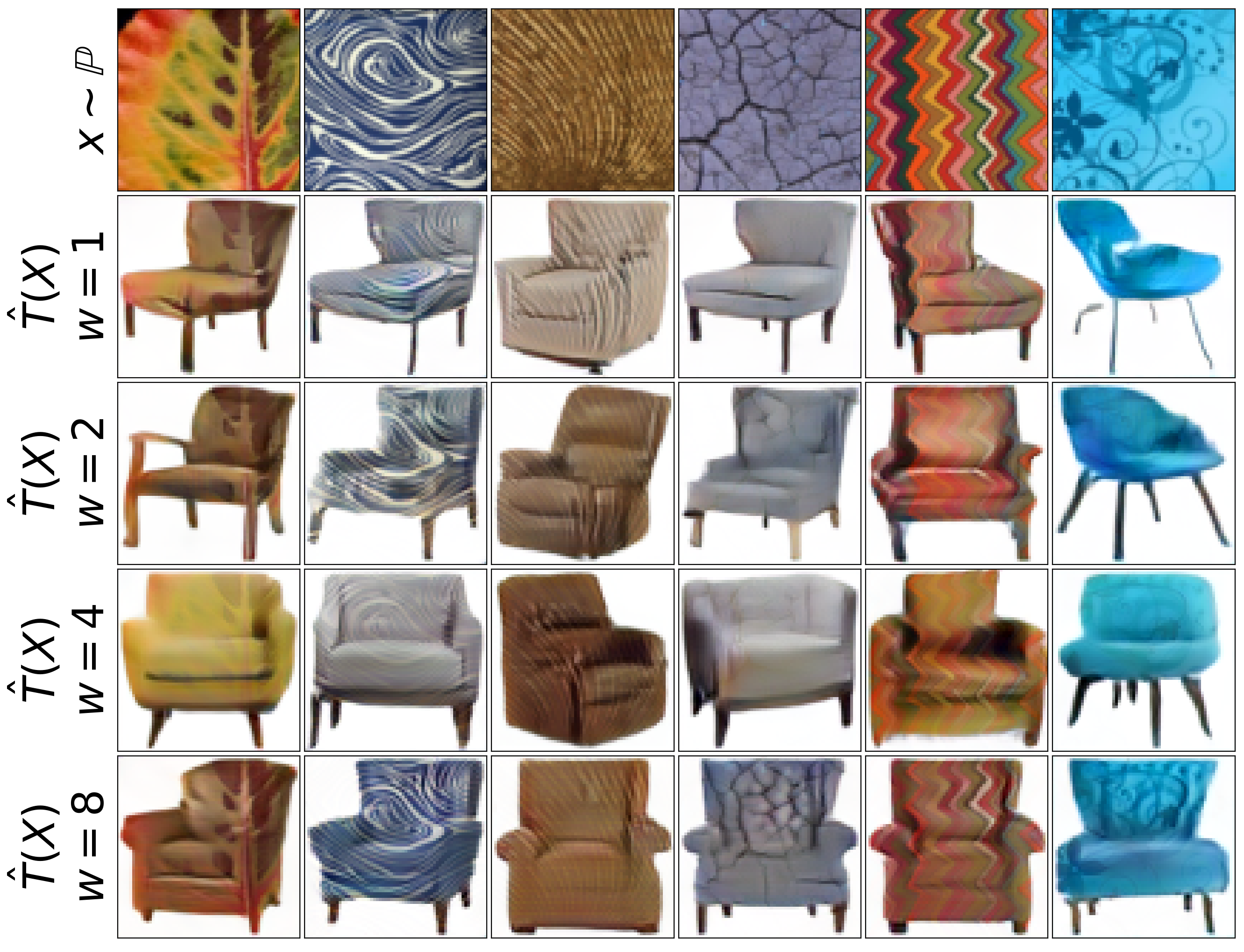
(a) IT results for textures $\rightarrow$ chairs (64$\times$64).

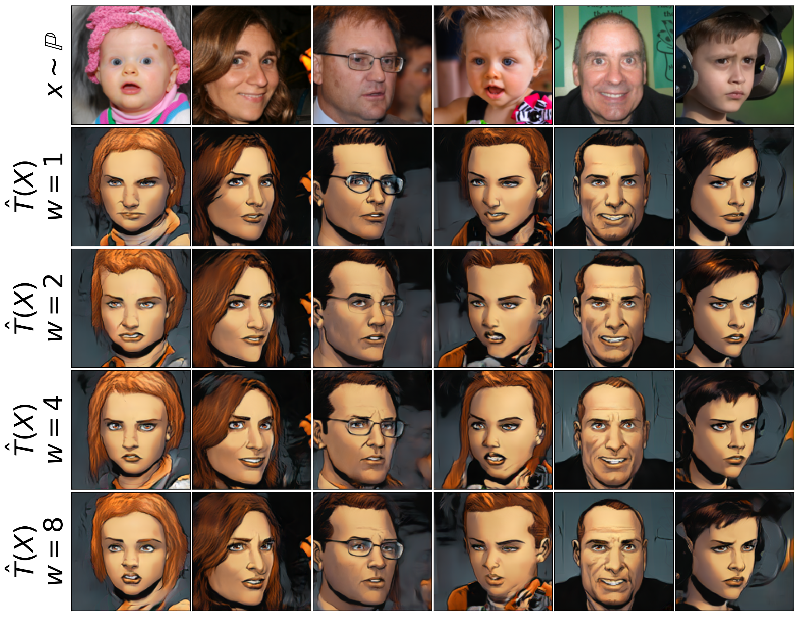
(b) IT results for ffhq $\rightarrow$ comics (128$\times$128).

Figure 9: Unpaired Translation with our Incomplete Transport.

Experiment	$w=1$	$w=2$	$w=4$	$w=8$
celeba $\rightarrow$ anime	0.297	0.154	0.133	0.094
handbag $\rightarrow$ shoes	0.368	0.320	0.259	0.252
textures $\rightarrow$ chairs	0.603	0.516	0.474	0.408
ffhq $\rightarrow$ comics	0.224	0.220	0.200	0.196

(a) Test $\ell^{2}$ transport cost of our learned IT maps.

Experiment	$w=1$	$w=2$	$w=4$	$w=8$
celeba $\rightarrow$ anime	14.65	20.79	22.18	22.84
handbag $\rightarrow$ shoes	27.10	29.70	42.90	53.80
textures $\rightarrow$ chairs	N/A	N/A	N/A	N/A
ffhq $\rightarrow$ comics	20.95	22.38	22.77	23.67

(b) Test FID of our learned IT maps.

Table 1: Test $\ell^{2}$ cost and FID of our learned IT maps.

Image datasets. We utilize the following publicly available datasets as $\mathbb{P},\mathbb{Q}$: celebrity faces [46], aligned anime faces, flickr-faces-HQ [36], comic faces, Amazon handbags from LSUN dataset [68], shoes [67], textures [16] and chairs from Bonn furniture styles dataset [1]. The sizes of datasets are from 5K to 500K samples. We work with $64\times 64$ and $128\times 128$ images.

Train-test split. We use 90% of each dataset for training. The remaining 10% are held for test. All the presented qualitative and quantitative results are obtained for test images.

Experimental results. Our evaluation shows that with the increase of $w$ the images $\hat{T}(x)$ translated by our IT method become more similar to the respective inputs $x$ w.r.t. $\ell^{2}$. In Table 1(a), we quantify this effect. Namely, we show that the test transport cost $\frac{1}{N_{\text{test}}}\sum_{n=1}^{N_{\text{test}}}c\big{(}x,\hat{T}(x)\big{)}$ decreases with the increase of $w$ which empirically verifies our Theorem 2.

We qualitatively demonstrate this effect in Fig. 1(b), 1(a), 9(b), 9(a) and 8. In celeba (female) $\rightarrow$ anime (Fig. 1(b)), the hair and background colors of the learned anime images become closer to celebrity faces’ colors with the increase of $w$. For example, in the 4th column of Fig. 1(b), the anime hair color changes from green to brown, which is close to that of the respective celebrity. In the 6th column, the background is getting darker. In handbag$\rightarrow$shoes (Fig. 1(a)), the color, texture and size of the shoes become closer to that of handbag. Additionally, for this experiment we plot the projections of the learned IT maps to the first 2 principal components of $\mathbb{Q}$ (Fig. 8). We see that projections are close to $\mathbb{Q}$ for $w=1$ and become closer to $\mathbb{P}$ with the increase of $w$. In ffhq$\rightarrow$comics, the changes mostly affect facial expressions and individual characteristics. In textures$\rightarrow$chairs, the changes are mostly related to chairs’ size which is expected since we use pixel-wise $\ell^{2}$ as the cost function. Additional qualitative results are given in Appendix G.5 (Fig. 24, 25, 9(a)).

For completeness, we measure test FID [32] of the translated samples, see Table 1(b). We do not calculate FID in the handbag$\rightarrow$chairs experiment because of too small sizes of the test parts of the datasets (500 textures, 2K chairs). However, we emphasize that FID is not representative when $w>1$. In this case, IT maps learn by construction only a part of the target measure $\mathbb{Q}$. At the same time, FID tests how well the transported samples represent the entire target distribution and is very sensitive to mode dropping [48, Fig. 1b]. Therefore, while the cost decreases with the growth of $w$, FID, on the contrary, increases. This is expected since IT maps to smaller part of $\mathbb{Q}$. Importantly, the visual quality of the translated images $\hat{T}(x)$ is not decreasing.

In Appendix C, we compare our IT method with other image-to-image translation methods and show that IT better preserves the input-output similarity.

6 Potential Impact

Inequality constraints for generative models. The majority of optimization objectives in generative models (GANs, diffusion models, normalizing flows, etc.) enforce the equality constraints, e.g., $T\sharp\mathbb{P}=\mathbb{Q}$, where $T\sharp\mathbb{P}$ is the generated measure and $\mathbb{Q}$ is the data measure. Our work demonstrates that it is possible to enforce inequality constraints, e.g., $T\sharp\mathbb{P}\leq w\mathbb{Q}$, and apply them to a large-scale problem. While in this work we primarily focus on the image-to-image translation task, we believe that the ideas presented in our paper have several visible prospects for further improvement and applications. We list them below.

(1) Partial OT. Learning alignments between measures of unequal mass is a pervasive topic which has already perspective applications in biology to single-cell data [66, 47, 19]. The mentioned works use unbalanced OT [14]. This is an unconstrained problem where the mass spread is softly controlled by the regularization. Therefore, may be hard to control how the mass is actually distributed. Using partial OT which enforces hard inequality constraints might potentially soften this issue. Our IT problem (12) is a particular case of partial OT (4). We believe that our study is useful for future development of partial OT methods.

(2) Generative nearest neighbors. NNs play an important role in machine learning applications such as, e.g., image retrieval [6]. These methods typically rely on fast discrete approximate NN [50, 35] and perform matching with the latent codes of the train samples. In contrast, nowadays, with the rapid growth of large generative models such as DALL-E [58], CLIP [57], GPT-3 [9], it becomes relevant to perform out-of-sample estimation, e.g., map the latent vectors to new vectors which are not present in the train set to generate new data. Our IT approach (for $w\rightarrow\infty$) is a theoretically justified way to learn approximate NN maps exclusively from samples. We think our approach might acquire applications here as well, especially since there already exist ways to apply OT in latent spaces of such models [20].

(3) Robustness and outlier detection. Our IT aligns the input measure $\mathbb{P}$ only with a part of the target measure $\mathbb{Q}$. This property might be potentially used to make the learning robust, e.g., ignore outliers in the target dataset. Importantly, the choice of outliers and contamination level are tunable via $c(x,y)$ and $w$, but their selection may be not obvious. At the same time, the potential $f^{*}$ vanishes on the outliers, i.e., samples in $\text{Supp}(\mathbb{Q})$ to which the mass is not transported.

Proposition 4 (The potential vanishes at outliers).

Under the assuptions of Theorem 5, the equality $f^{*}(y)=0$ holds for all $y\in\text{Supp}(\mathbb{Q})\setminus\text{Supp}(T^{*}\sharp\mathbb{P})$.

We empirically illustrate this statement in Appendix A. As a result of this proposition, a possible byproduct of our method is an outlier-score $f^{*}(y)$ for the target data. Such applications of OT are promising and there already exist works [52, 7, 54] developing approaches to make OT more robust.

Limitations, societal impact. We discuss limitations, societal impact of our study in Appendix A.

ACKNOWLEDGEMENTS. This work was partially supported by Skoltech NGP Program (Skoltech-MIT joint project).

Appendix A Limitations

Transport costs. Our theoretical results hold true for any continuous cost function $c(x,y)$, but our experimental study uses $\ell^{2}$ as it already yields a reasonable performance in many cases. Considering more semantically meaningful costs for image translation, e.g., perceptual [70], is a promising future research direction.

Intersecting supports. ET is the nearest neighbor assignment (3.1). Using ET may be unreasonable when $\mathcal{X}=\mathcal{Y}$ and $\text{Supp}(\mathbb{P})$ intersects with $\text{Supp}(\mathbb{Q})$. For example, if $c(x,y)$ attains minimum over $y\in\mathcal{Y}$ for a given $x\in\mathcal{X}$ at $x=y$, e.g., $c=\ell^{2}$, then there exists a ET plan satisfying $\pi^{*}(y|x)=\delta_{x}$ for all $x\in\text{Supp}(\mathbb{P})\cap\text{Supp}(\mathbb{Q})$. It does not move the mass of points $x$ in this intersection. We provide an illustrative toy 2D example in Fig. 10(b).

Limited diversity. It is theoretically impossible to preserve input-output similarity better than ET maps. Still one should understand that in some cases these maps may yield degenerate solutions. In Fig. 10(a), we provide a toy 2D example of an IT map ($w=8$) which maps all inputs to nearly the same point. In Fig. 9(a) (texture $\rightarrow$ chair translation), we see that with the increase of $w$ the IT map produces less small chairs but more large armchairs. In particular, when $w=8$, only armchairs appear, see Fig. 9(a). This is because they are closer (in $\ell^{2}$) to textures due to having smaller white background area.

(a) Limited diversity. The true ET map is degenerate: it maps the entire $\mathbb{P}$ to a single vertex of the triangle $\mathbb{Q}$. The example shows the learned IT map with high $w=20$ approximating the ET map.

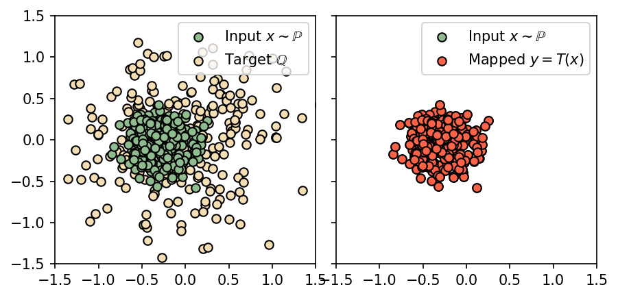
(b) Intersecting supports. The true ET map is the identity map: it does not move the probability mass of $\mathbb{P}$. The example shows the learned IT map with high $w=8$ approximating the ET map.

Figure 10: Toy 2D examples showing two (potential) limitations of IT maps.

Unused samples. Doing experiments, we noticed that the model training slows down with the increase of $w$. A possible cause of this is that some samples from $\mathbb{Q}$ become non-informative for training (this follows from our Proposition 4). Intuitively, the part of $\text{Supp}(\mathbb{Q})$ to which the samples of $\mathbb{P}$ will not be mapped to is not informative for training. We illustrate this effect on toy ’Wi-Fi’ example and plot the histogram of values of $f^{*}$ in Fig. 11. One possible negative of this observation is that the training of IT maps or, more generally, partial OT maps, may naturally require larger training datasets.

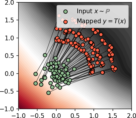
(a) Surface of $f^{*}$(trained with $w=1$).

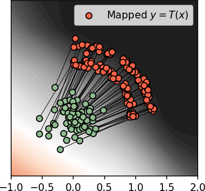
(b) Surface of $f^{*}$(trained with $w=\frac{3}{2}$).

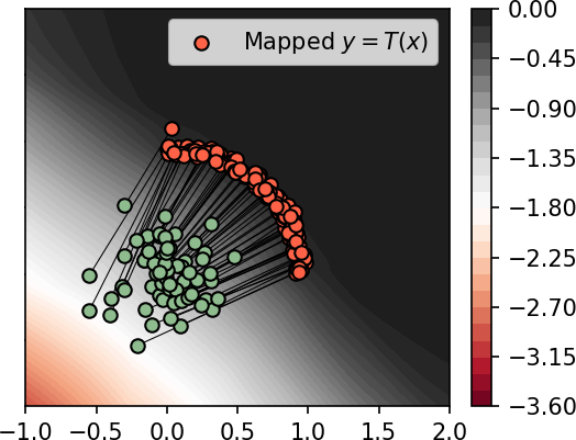
(c) Surface of $f^{*}$(trained with $w=3$).

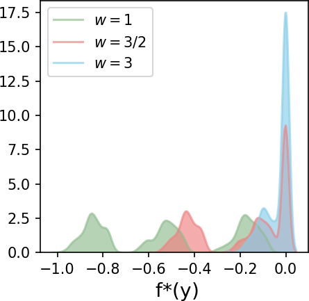
(d) Histograms of valuesof $f^{*}(y)$ for $y\sim\mathbb{Q}$.

Figure 11: Illustration the unused samples. In Figures 11(a), 11(b), 11(c), we visualize the surface of the learned potential $f^{*}$ on the ’Wi-Fi’ example and $w\in\{1,\frac{3}{2},3\}$. In Figures 11(b), 11(c), the potential vanishes on the arcs of $\mathbb{Q}$ to which the mass of $\mathbb{P}$ is not mapped, i.e., $f^{*}(y)=0$. In Figure 11(d), we plot the distribution of values of $f^{*}(y)$ for $y\sim\mathbb{Q}$. For $w\in\{\frac{3}{2},3\}$, we see large pikes around $f^{*}(y)=0$ further demonstrating that the potential equals to zero on a certain part of $\mathbb{Q}$.

Limited quantitative metrics. In experiments (5), we use a limited amount of quantitative metrics. This is because existing unpaired metrics, e.g., FID [32], KID [8], etc., are not suitable for our setup. They aim to test equalities, such as $T\sharp\mathbb{P}=\mathbb{Q}$, while our learned maps disobey it by the construction (they capture only a part of $\mathbb{Q}$). Developing quality metrics for partial generative models is an important future research direction. Meanwhile, for our method, we have provided a toy 2D analysis (5.1) and explanatory metrics (5.2), such as the transport cost (Table 1(a)).

Inexistent IT maps. The actual IT plans between $\mathbb{P},\mathbb{Q}$ may be non-deterministic, while our approach only learns a deterministic map $T$. Nevertheless, thanks to our Proposition 3, for every $\epsilon>0$ there always exists a 1-to-1 map $T_{\epsilon}\sharp\mathbb{P}\leq w\mathbb{Q}$ which provides $\epsilon$-sub-optimal cost $\int_{\mathcal{X}}c\big{(}x,T_{\epsilon}(x)\big{)}d\mathbb{P}(x)\leq\text{Cost}_{w}(\mathbb{P},\mathbb{Q})+\epsilon$. Thus, IT cost (12) can be approached arbitrary well with deterministic transport maps. A potential way to modify our algorithm is to learn stochastic plans is to add random noise $z$ to generator $T(x,z)$ as input, although this approach may suffer from ignoring $z$, see [43, 5.1].

Fake solutions and instabilities. Lagrangian objectives such as (15) may potentially have optimal saddle points $(f^{*},T^{*})$ in which $T^{*}$ is not an OT map. Such $T^{*}$ are called fake solutions [42] and may be one of the causes of training instabilities. Fake solutions can be removed by considering OT with strictly convex weak costs functions [43, Appendix H], see Appendix G.2 for examples.

Potential societal impact. Neural OT methods and, more generally, generative models are a developing research direction. They find applications such as style translation and realistic content generation. We expect that our method may improve existing applications of generative models and add new directions of neural OT usage like outlier detection. However, it should be taken into account that generative models can also be used for negative purposes such as creating fake faces.

Appendix B Toy 2D Illustrations of Other Methods

In this section, we demonstrate how the other methods perform in ’Wi-Fi’ and ’Accept’ experiments. We start with ’Wi-Fi’. Assume that we would like to map $\mathbb{P}$ to the closest $\frac{2}{3}$-rd fraction of $\mathbb{Q}$, i.e., we aim to learn 2 of 3 arcs in $\mathbb{Q}$, (as in Fig. 7(c)).

In Fig. 12(d), we show the discrete partial OT (4) [11] with parameters $w_{0}\!=\!m\!=\!1$, $w_{1}\!=\!\frac{3}{2}$, corresponding to IT (12) with $w=\frac{3}{2}$. To obtain the discrete matching, we run ot.partial.partial_wasserstein2 from POT. As expected, it matches the input $\mathbb{P}$ with $\frac{2}{3}$ of $\mathbb{Q}$ and can be viewed as the ground truth (coinciding with our Fig. 7(c)).

First, we show the GAN [27] endowed with additional $\ell^{2}$ loss with weight $\lambda=0.5$ (in Fig. 12(a)). Next, we consider discrete unbalanced OT [14] with the quadratic cost $c=\ell^{2}$. In Fig. 12(b), we show the results of the matching obtained by ot.unbalanced with parameters $m=1,reg=0.1$, $reg_{m}=1$, $numItermax=200000$. Additionally, in Fig. 12(c) we show the result of neural unbalanced OT method [66]. To make their unbalanced setup maximally similar to our IT, we set to zero their regularization parameters. The rest parameters are default except for $\lambda_{0}=0.02$ ($\ell^{2}$ loss parameter), $\lambda_{2}=5$ (input and target measures’ variation parameter).

We see that GAN$+\ell^{2}$ (Fig. 12(a)) and unbalanced OT (Fig. 12(b) and 12(c)) indeed match $\mathbb{P}$ with only a part of the target measure $\mathbb{Q}$. The transported mass is mostly concentrated in the two small arcs of $\mathbb{Q}$ which are closest to $\mathbb{P}$ w.r.t. $\ell^{2}$ cost. The issue here is that some mass of $\mathbb{P}$ spreads over the third (biggest) arc of $\mathbb{Q}$ yielding outliers. This happens because unbalanced OT (GAN can be viewed as its particular case) is an unconstrained problem: the mass spreading is controlled via soft penalization ($f$-divergence loss term). The lack of hard constraints, such as those in partial OT (4) or IT (12), makes it challenging to strictly control how the mass in unbalanced OT actually spreads.

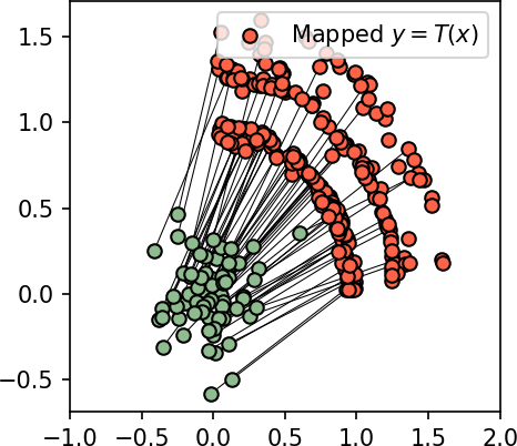
(a) GAN$+\ell^{2}$.

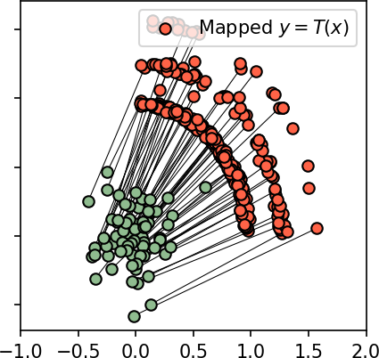
(b) Discrete unbalanced OT.

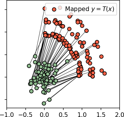
(c) Scalable unbalanced OT.

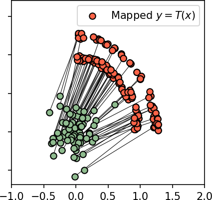
(d) Discrete Partial OT(desired ground truth).

Figure 12: Transport maps learned by various methods in ’Wi-Fi’ experiment (Fig. 7(a)).

For completeness, we also show the results of these methods applied to ’Accept’ experiment, see Fig. 13. Here we tested various hyperparameters for these methods but did not achieve the desired behaviour, i.e., learning only the text ’Accept’. Moreover, we noted that GAN$+\ell^{2}$ for large $\lambda$ yields undesirable artifacts (Fig. 13(a)). This is because GAN and $\ell^{2}$ losses contradict to each other and still the models tried to minimize them both. We further discuss in Appendix C below.

(a) GAN$+\ell^{2}$.

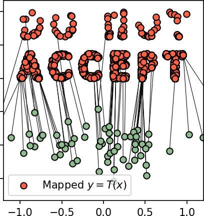
(b) Discrete unbalanced OT.

(c) Scalable unbalanced OT.

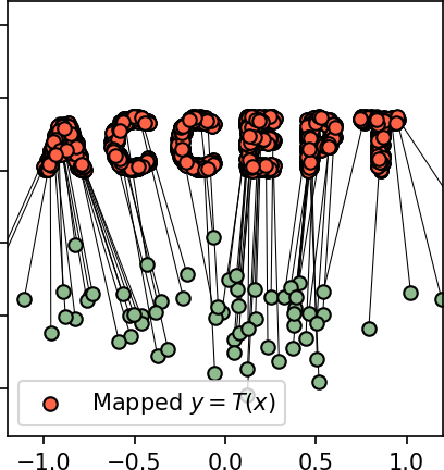
(d) Discrete Partial OT(desired ground truth).

Figure 13: Transport maps learned by various methods in ’Accept’ experiment.

Appendix C Comparison with Other Image-to-Image Translation Methods

Recall that ET by design is the best translation between a pair of domains w.r.t. the given dissimilarity function $c(x,y)$. Our IT maps with the increase of $w$ provide better input-output similarity and recover ET when $w\rightarrow\infty$ (3.3). A reader may naturally ask: (a) How else can we recover ET maps? (b) To which extent one can control the input-output similarity in existing translation methods? (c) Can these methods be used to approximate ET? We discuss these aspects below.

Many translation methods are based on GANs, see [55, 3, 13] for a survey. Their learning objectives are usually combined of several loss terms:

$$\mathcal{L}_{\text{Total}}(T)\stackrel{{\scriptstyle def}}{{=}}\mathcal{L}_{Dom}(T)+\lambda\cdot\mathcal{L}_{Sim}(T)+[\text{other terms}].$$ (17)

In (17), the domain loss $\mathcal{L}_{Dom}$ is usually the vanilla GAN loss involving a discriminator [27] ensuring that the learned map $x\mapsto T(x)$ transforms inputs $x\sim\mathbb{P}$ to the samples from the target data distribution $\mathbb{Q}$. The similarity loss $\mathcal{L}_{Sim}$ (with $\lambda\geq 0$) is usually the identity loss $\int_{\mathcal{X}}\|x-T(x)\|_{1}d\mathbb{P}(x)$. More generally, it can be an arbitrary unsupervised loss of the form $\int_{\mathcal{X}}c\big{(}x,T(x)\big{)}d\mathbb{P}(x)$ stimulating the output sample $T(x)$ to look like the input samples $x$ w.r.t. given dissimilarity function $c$, e.g., $\ell^{1},\ell^{2},\ell^{p}$, perceptual, etc. The other terms in (17) involve model-specific terms (e.g., cycle consistency loss in CycleGAN) which are not related to our study.

When learning a model via optimizing (17), a natural way to get better similarity of $x$ and $T(x)$ in (17) is to simply increase weight $\lambda$ of the corresponding loss term. This is a straightforward approach but it has a visible limitation. When $\lambda$ is high, the term $\lambda\cdot\mathcal{L}_{\text{Sim}}$ dominates over the other terms such as $\mathcal{L}_{\text{Dom}}$, and the model $T$ simply learns to minimize this loss ignoring the fact that the output sample should be from the target data distribution $\mathbb{Q}$. In other words, in (17) there is a nasty trade-off between $T(x)$ belonging to the target data distribution $\mathbb{Q}$ and input-output similarity of $x$ and $T(x)$. The parameter $\lambda\geq 0$ controls this realism-similarity trade-off, and we study how it affects the learned map $T$ below.

We pick CycleGAN [72] as a base model for evaluation since it is known as one of the principal models to solve the unpaired translation problem. We use $c=\ell^{1}$ as the similarity loss as the CycleGAN’s authors originally used in their paper. We consider parameter $\lambda\in[0,50,100,200,250,300,350,500]$.

Additionally, we perform comparison with a more recent StarGAN-v2 [15] model. By default, StarGAN-v2 does not use any similarity loss and does not enforce the output to be similar to the input. Therefore, analogously to CycleGAN, we endow the model with an additional $\ell^{1}$ similarity loss and consider $\lambda\in[0,1,10,50,100,200,500]$.

We train both models on celeba $\rightarrow$ anime ($64\times 64$) and handbags $\rightarrow$ shoes ($128\times 128$) translation with various $\lambda$ and report the qualitative and quantitative results below. In all the cases, we report both $\ell^{2}$ and $\ell^{1}$ transport costs and FID on the test samples. Tables 2, 3, 4, 5 show transport costs and FID of GANs. FID and $\ell^{2}$ metrics for our method are given in the main text (Tables 1(b), 1(a)) and $\ell^{1}$ cost is given in Table 6 below. For convenience, we visualize $(\text{FID},\text{Cost})$ pairs for our method and GANs in Fig. 14(a).

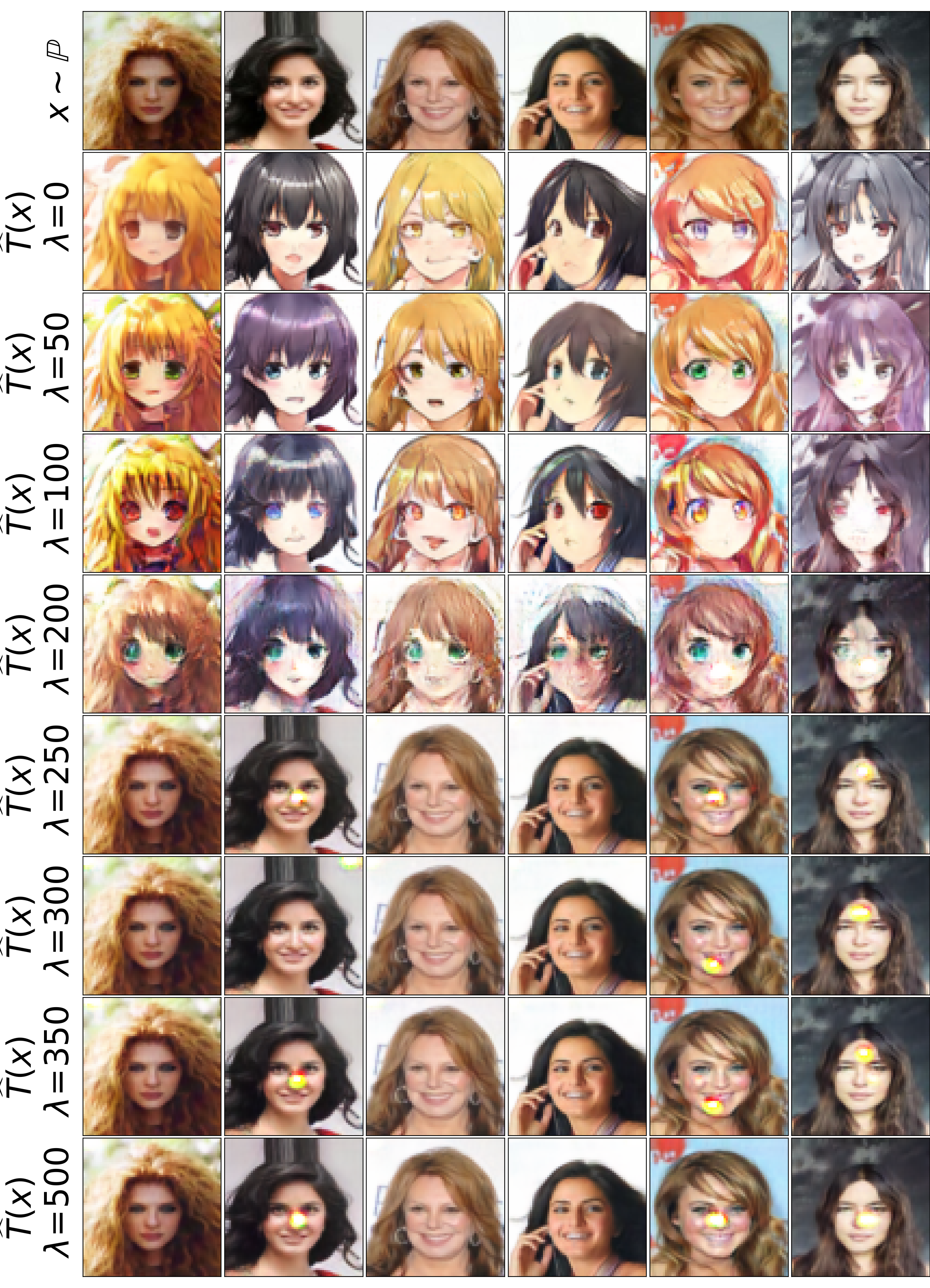
(a) Celeba (female) $\rightarrow$ anime (64$\times$64).

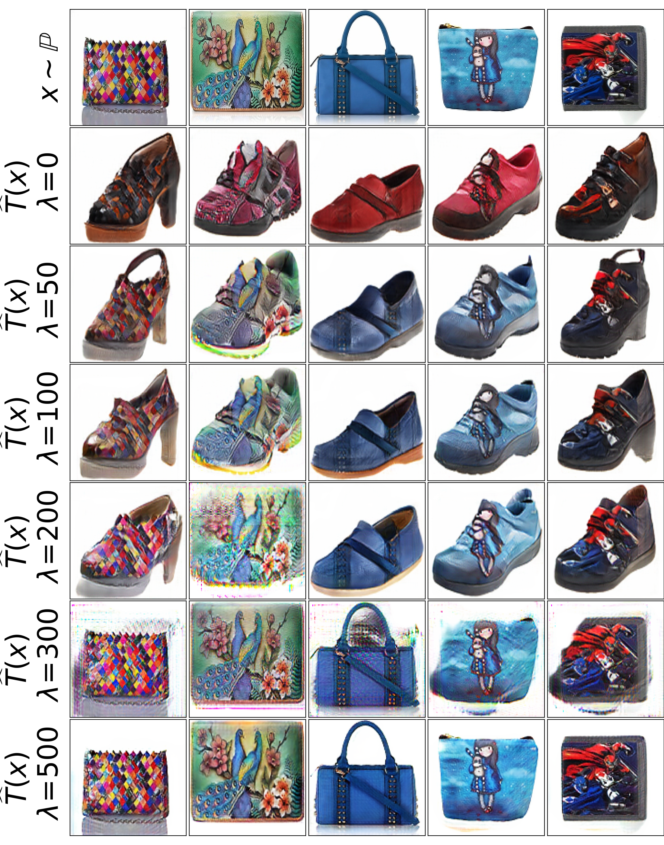
(b) Handbags $\rightarrow$ shoes (128$\times$128).

Figure 15: Unpaired translation via CycleGAN endowed with $\ell^{1}$ identity loss with various weights $\lambda$.

Results and discussion (CycleGAN). Interestingly, we see that for CycleGAN adding small identity loss $\lambda=50$ yields not only decrease of the transport cost (compared to $\lambda=0$), but some improvement of FID as well. Still we see that the transport cost in CycleGAN naturally decreases with the increase of weight $\lambda$. Unfortunately, this decrease is accompanied by the decrease of the visual image quality, see Fig. 15. While for large $\lambda$ the cost for CycleGAN is really small, the model is practically useless since it poors image quality. For very large $\lambda$, CycleGAN simply learn the identity map, as expected.

For $\lambda$ providing acceptable visual quality, CycleGAN yields a transport cost which is bigger than that of standard OT $(w=1)$. Our result for $w=8$ is unachievable for it. Note that in most cases FID of our IT method is smaller than that of CycleGAN.

Results and discussion (StarGAN-v2). In the celeba$\rightarrow$anime experiment, StarGAN-v2 results are similar to CycleGAN ones. Our IT with $w=2$ easily provides smaller transport cost (better similarity) than StarGAN-v2. In the handbags $\rightarrow$ shoes translation, we have encountered surprising observations. We see that starting from $\lambda=10$ the model fails to translate some of the handbags to shoes, i.e., these handbags remain nearly unchanged. We notice the similar behaviour for vanilla GAN in ’Accept’ experiment, see Fig. 13(a). This explains the low cost for StarGAN-v2 model ($\lambda\geq 10$). Surprisingly to us, for $\lambda=10$, FID metric is also low despite the fact that model frequently produces failures, see the highlighted results in Fig. 16. Note that while FID is a widely used metric, it still could produce misleading estimations which we observe in the latter case.

Additionally, we provide a large set of randomly generated images for $\lambda=10$ to qualitatively show that the stated issue is indeed notable, see Fig. 17. These failures demonstrate the limited practical usage of the model. Our IT method does not suffer from this issue which we qualitatively demonstrate on the same set of images for different weights $w$, see Fig. 25.

Experiment	Cost	$\lambda=0$	$\lambda=50$	$\lambda=100$	$\lambda=200$	$\lambda=250$	$\lambda=300$	$\lambda=350$	$\lambda=500$
celeba $\rightarrow$ anime	$\ell^{1}$	0.48	0.48	0.39	0.26	0.09	0.09	0.09	0.09
handbag $\rightarrow$ shoes		0.42	0.36	0.34	0.31	0.32	0.22	0.16	0.07
celeba $\rightarrow$ anime	$\ell^{2}$	0.33	0.32	0.24	0.11	0.01	0.02	0.02	0.01
handbag $\rightarrow$ shoes		0.51	0.43	0.41	0.35	0.37	0.22	0.14	0.02

Table 2: Test $\ell^{1}$ and $\ell^{2}$ transport cost of CycleGAN.

Experiment	$\lambda=0$	$\lambda=50$	$\lambda=100$	$\lambda=200$	$\lambda=250$	$\lambda=300$	$\lambda=350$	$\lambda=500$
celeba $\rightarrow$ anime	22.9	20.8	35.2	88.8	122.2	123.5	120.0	122.8
handbag $\rightarrow$ shoes	27.8	23.4	23.6	37.4	38.5	105.6	144.9	152.9

Table 3: Test FID of CycleGAN.

Experiment	Cost	$\lambda=0$	$\lambda=1$	$\lambda=10$	$\lambda=50$	$\lambda=100$	$\lambda=200$	$\lambda=500$
celeba $\rightarrow$ anime	$\ell^{1}$	0.672	0.355	0.210	0.076	0.050	0.030	0.029
handbag $\rightarrow$ shoes		0.562	0.465	0.244	0.087	0.068	0.054	0.048
celeba $\rightarrow$ anime	$\ell^{2}$	0.686	0.216	0.094	0.017	0.006	0.002	0.002
handbag $\rightarrow$ shoes		0.739	0.584	0.244	0.040	0.023	0.015	0.012

Table 4: Test $\ell^{1}$ and $\ell^{2}$ transport costs of StarGAN-v2.

Experiment	$\lambda=0$	$\lambda=1$	$\lambda=10$	$\lambda=50$	$\lambda=100$	$\lambda=200$	$\lambda=500$
celeba $\rightarrow$ anime	19.55	22.40	42.30	99.68	123.76	137.8	139.11
handbag $\rightarrow$ shoes	25.45	45.13	22.36	131.8	149.8	155.8	158.8

Table 5: Test FID of StarGAN-v2.

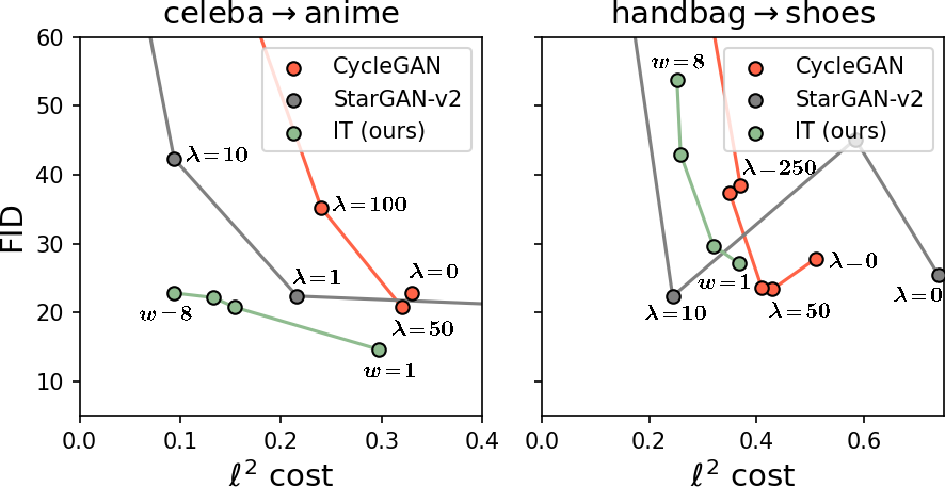
(a) Test $\ell^{2}$ transport cost.

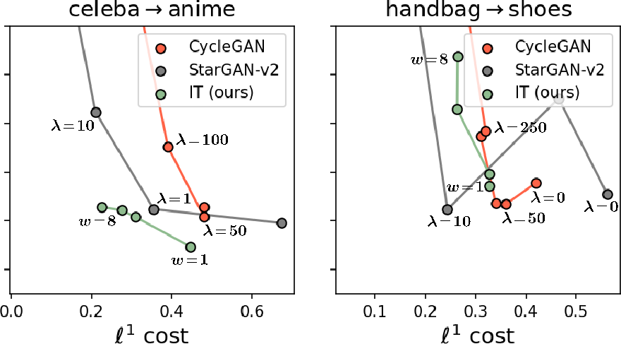
(b) Test $\ell^{1}$ transport cost.

Figure 14: Comparison of test FID and transport costs ($\ell^{2}$ and $\ell^{1}$) of our IT method and CycleGAN.

 

Experiment	$w=1$	$w=2$	$w=4$	$w=8$
celeba $\rightarrow$ anime	0.447	0.309	0.275	0.225
handbag $\rightarrow$ shoes	0.327	0.328	0.263	0.264

Table 6: Test $\ell^{1}$ transport cost of our IT maps (learned with $\ell^{2}$ transport cost).

Concluding remarks. Our algorithm with $w\rightarrow\infty$ allows us to achieve better similarity without the decrease of the image quality. At the same time, GANs fail to do this when $\lambda\rightarrow\infty$. Why?

We again emphasize that typical GAN objective (17) consists of several loss terms. Each term stimulates the model to attain certain properties (realism, similarity to the input, etc.). These terms, in general, contradict each other as they have different minima $T$. This yields the nasty trade-off between the loss terms. Our analysis shows that conceptually there is no significant difference between CycleGAN and a more recent StarGAN-v2 model. More generally, any GAN-based method inherits realism-similarity tradeoff issue. GANs’ differences are mostly related to the use of other architectures or additional losses. Therefore, we think that additional comparisons are excessive since they may not provide any new insights.

In contrast, our method is not a sum of losses. Our objective (15) may look like a direct sum of a transport cost with an adversarial loss; our method does have a generator (transport maps $T$) and a discriminator (potential $f$) which are trained via the saddle-point optimization objective $\max_{f}\min_{T}$. Yet, this visible similarity to GAN-based methods is deceptive. Our objective $\max_{f}\min_{T}$ can be viewed as a Lagrangian and is atypical for GANs: the generator is in the inner optimization problem $\min_{T}$ while in GANs the objective is $\min_{T}\max_{f}$. In our case, similar to other neural dual OT methods, the generator is adversarial to the discriminator but not vice versa, as in GANs. Please consult [43, 4.3], [24] or [20] for further discussion about OT methods.

GANs aim to balance loss terms $\mathcal{L}_{\text{Dom}}$ and $\mathcal{L}_{\text{Sim}}$. Our optimization objective enforces the constraint $T\sharp\mathbb{P}\leq w\mathbb{Q}$ via learning the potential $f$ (a.k.a. Lagrange multiplier) and among admissible maps $T$ searches for the one providing the smallest transport cost. There is no realism-similarity trade-off. For completeness, we emphasize that when $w\rightarrow\infty$, FID in Table 1(b) does not drop because of the decrease of the image quality, but because our method covers the less part of $\mathbb{Q}$. FID negatively reacts to this [48, Fig. 1b].

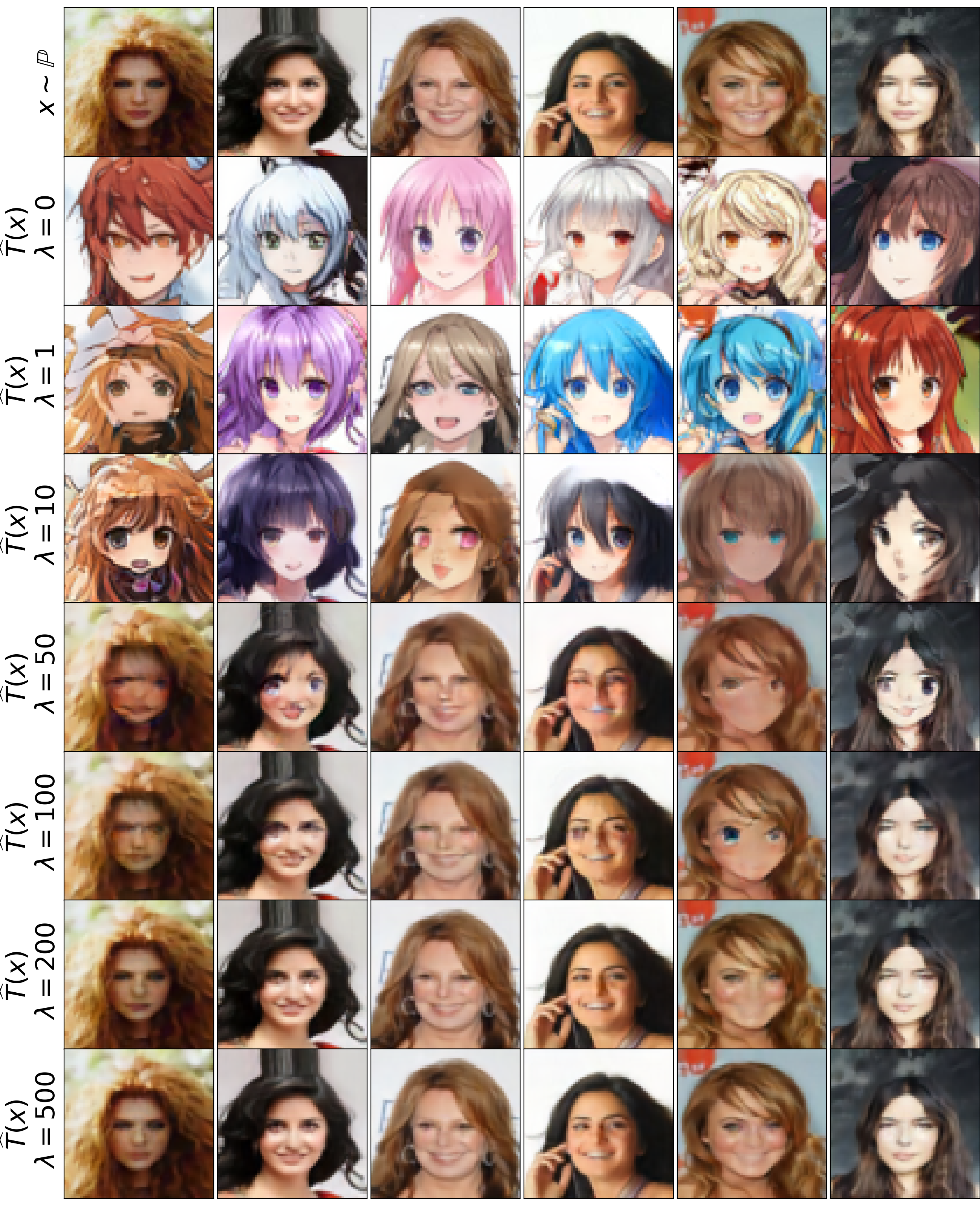
(a) Celeba (female) $\rightarrow$ anime (64$\times$64).

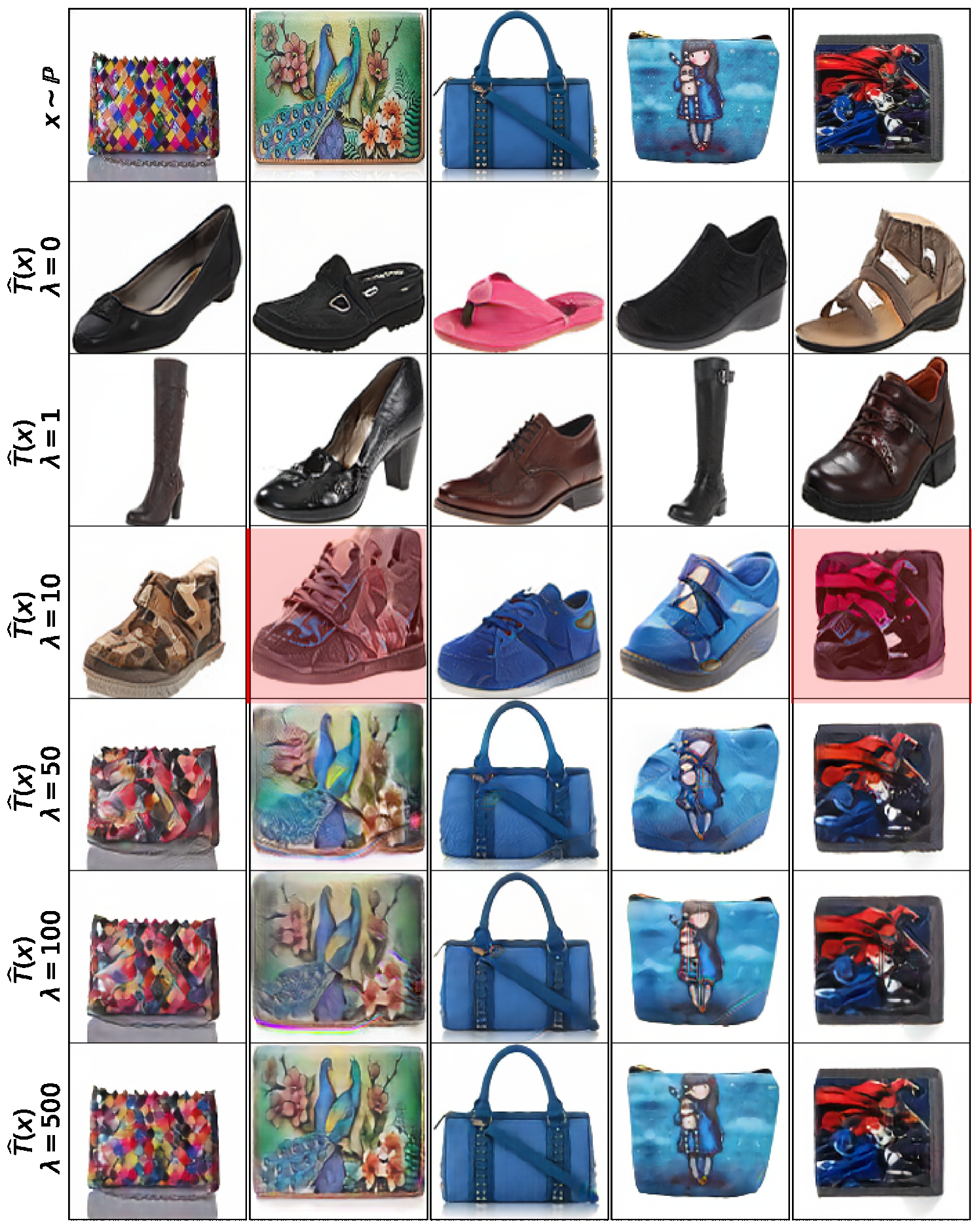
(b) Handbags$\rightarrow$ shoes (128$\times$128).

Figure 16: Unpaired translation via StarGAN-v2 endowed with $\ell^{1}$ identity loss with various weights $\lambda$.

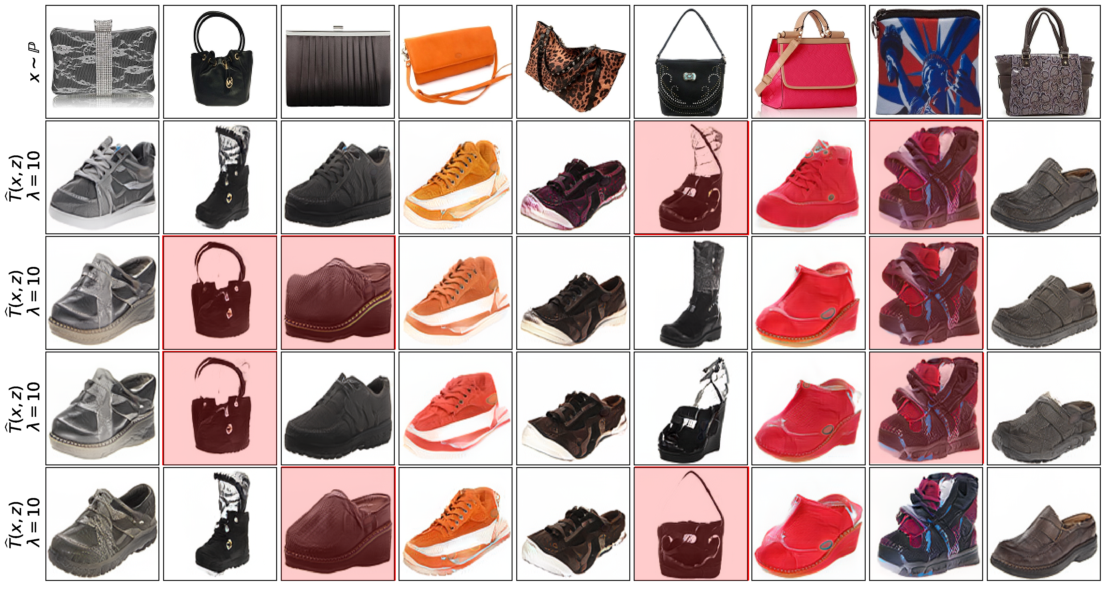
Figure 17: Unpaired translation of handbags to shoes (128$\times$128) via StarGAN-v2 endowed with $\ell^{1}$ identity loss ($\lambda=10$). Since StarGAN-v2 is a stochastic (one-to-many) approach, we visualize several generated samples for different noise vectors $z$. Failures (poorly translated handbags which remain nearly unchanged) are highlighted with red.

Appendix D Relation and Comparison with Discrete Partial OT Methods

The goal of domain translation is to recover the map $x\mapsto T(x)$ between two domains $\mathbb{P}$, $\mathbb{Q}$. We approach this problem by approximating $T$ with a neural network trained on the empirical samples $X=\{x_{1},\dots,x_{N}\}$, $Y=\{y_{1},\dots,y_{M}\}$, i.e., train datasets. Our method generalizes to new (previously unseen, test) input samples $x_{new}\sim\mathbb{P}$, i.e, our learned map $\widehat{T}$ can be applied to new input samples to generate new target samples $\widehat{T}(x_{new})$.

In contrast, discrete OT methods (including discrete partial OT) perform a matching between the empirical distributions $\widehat{\mathbb{P}}_{N}=\sum_{n=1}^{N}\delta_{x_{n}},\widehat{\mathbb{Q}}_{M}=\sum_{m=1}^{M}\delta_{y_{m}}$. Thus, they do not provide out-of-sample estimation of the transport plan $\pi(y|x_{new})$ or map $T(x_{new})$. The reader may naturally wonder: why not to interpolate the solutions of discrete OT? For example, a common strategy is to derive barycentric projections $\overline{T}(x)=\int_{\mathcal{Y}}yd\pi(y|x)$ of the discrete OT plan $\pi$ and then learn a network $T_{\theta}(x)\approx\overline{T}(x)$ to approximate them [63]. Below we study this approach and show that it does not provide reasonable performance.

We perform evaluation of the BP approach on celeba$\rightarrow$anime translation. We solve the discrete partial OT (DOT) between the parts of the train data $X$ (11K samples), $Y$ (50K samples). We use ot.partial.partial_wasserstein algorithm with parameters $w_{0}=m=1$ and vary $w_{1}\in\{1,2,4,8\}$, see the notation in (4). This corresponds to our IT (12) with $w=w_{1}$. Then we regress a UNet $T_{\theta}$ to recover the barycentric projection $\overline{T}$. We also simulate the case of $w=\infty$ by learning the discrete NNs in the train dataset using NearestNeighbors algorithm from sklearn.neighbors. We experiment with using MSE or VGG-based perceptual error as the loss function for regression. We visualize the obtained results in Fig. 18 and report average $\ell^{2}$ test transport cost, FID in Table 7.

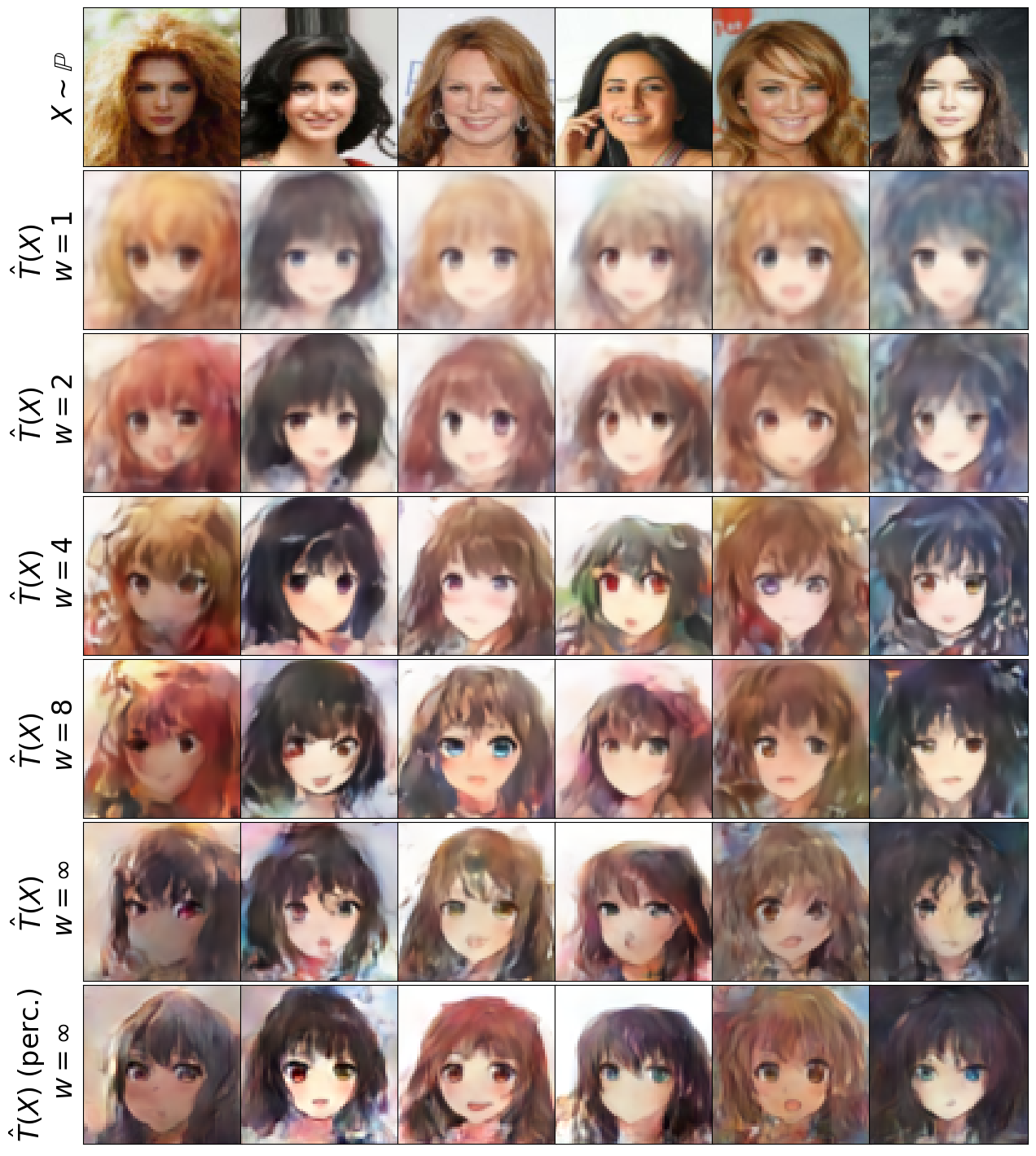
(a) Results on test set.

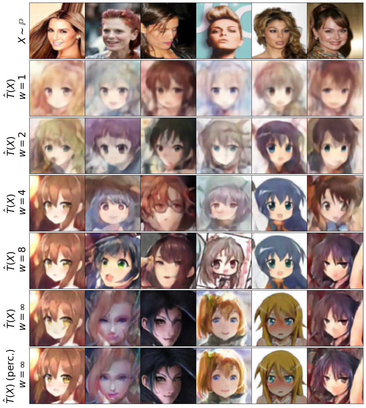
(b) Results on train set.

Figure 18: Unpaired translation with DOT+BP in celeba$\rightarrow$ anime experiment visualized on test, train partitions.

Metrics	$w=1$	$w=2$	$w=4$	$w=8$	$w=\infty$	$w=\infty$ (perc.)
$\ell^{2}$ cost	0.298	0.199	0.184	0.167	0.158	0.165
FID	185.35	137.53	82.67	82.19	82.24	82.45

Table 7: Test $\ell^{2}$ cost, FID of the DOT+BP method trained with $\ell^{2}$ or perceptual loss function.

BP methods are known not to work well in large scale problems such as unpaired translation because of the averaging effect, see Figure 3 and large FID values of BP in Table 1 of [17]. Indeed, one may learn a barycentric projection network $T_{\theta}(x)\approx\int_{\mathcal{Y}}yd\pi(y|x)$ over the discrete OT plan $\pi$, yet it is clear that $\int_{\mathcal{Y}}yd\pi(y|x)$ is a direct weighted average of several images $y$, i.e., some blurry average image of poor quality. It is not satisfactory for practical applications.

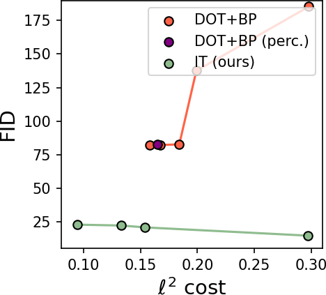
Figure 19: Test FID, $\ell^{2}$ costof our IT vs. DOT+BP.

Our qualitative results indeed show that BP approach for small $w$ leads to the averaging effect. We see that on the train dataset this effect disappears with the increase of $w$, see Fig. 18(b). It is expected, since with the increase of weight the conditional distribution of a plan $\pi(y|x)$ tends to a degenerate distribution concentrated at the nearest neighbor $NN(x)$ of $x$ in the train dataset, i.e., $\pi(y|x)\approx\delta_{NN(x)}$ when $w\rightarrow\infty$. This means, that in the limit the barycentric projection in point $x$ is its nearest neighbor $NN(x)$.

However, the learned network ($w=\infty$) does not generalize well to unseen test samples and produces images of insufficient quality which is much worse than for the train samples, see Fig. 18(a). Despite the fact that test $\ell^{2}$ cost and FID decrease with the increase of $w$, see Table 7, Fig. 19, generated test images have poor quality for all weights $w$. Yet, the FID scores as well as the $\ell^{2}$ costs are much bigger than in our method in all the cases.

As the MSE error for regression is known not to work well in image tasks, we also conduct an experiment using the perceptual error function to learn $T_{\theta}$. Unfortunately, training the neural network with perceptual error does not lead to meaningful improvements, see the bottom lines of Fig. 18(b), 18(a), Table 7. This confirms that the origins of DOT+BP method’s poor performance lie not in the regression part, but in the entire methodology based on barycentric projections.

To conclude, discrete OT methods are not competitors to our work as there is no straightforward and well-performing way to make out-of-sample DOT estimation in large scale image processing tasks.

Appendix E Experimental Details

Pre-processing. For all datasets, we rescale images’ RGB channels to [-1, 1]. As in [40], we rescale aligned anime face images to 512$\times$512. Then we do 256$\times$256 crop with the center located 14 pixels above the image center to get the face. Finally, for all datasets except the textures dataset, we resize the images to the required size (64$\times$64 or 128$\times$128). We apply random horizontal flipping augmentation to the comic faces and chairs datasets. Analogously to [42], we rescale describable textures to minimal border size of 300, do the random resized crop (from 128 to 300 pixels) and random horizontal, vertical flips. Next, we resize images to the required size (64 $\times$ 64 or 128 $\times$ 128).

Neural networks. In 5.1, we use fully connected networks both for the mapping $T_{\theta}$ and potential $f_{\psi}$. In 5.2, we use UNet [60] architecture for the transport map $T_{\theta}$. We use WGAN-QC’s [45] ResNet [30] discriminator as a potential $f_{\psi}$. We add an additional final layer $x\mapsto-|x|$ to $f_{\psi}$ to make its outputs non-positive.

Optimization. We employ Adam [38] optimizer with the default betas both for $T_{\theta}$ and $f_{\psi}$. The learning rate is $lr=10^{-4}$. We use the MultiStepLR scheduler which decreases $lr$ by 2 after [(5+5$\cdot w$)K, (20+5$\cdot w$)K, (40+5$\cdot w$)K, (70+5$\cdot w$)K] iterations of $f_{\psi}$ where $w\in\{1,2,4,8\}$ is a weight parameter. The batch size is $|X|=256$ for toy ’Wi-Fi’, $|X|=4096$ for toy Accept, and $|X|=64$ for image-to-image translation experiments. The number of inner $T_{\theta}$ iterations is $k_{T}=10$. In toy experiments, we observe convergence in $\approx$ 30K total iterations of $f_{\psi}$ for ’Wi-Fi’, in $\approx$ 70K for Accept. In the image-to-image translation, we do $\approx$ 70K iterations for 128 $\times$128 datasets, $\approx$ 40K iterations for 64$\times$64 datasets. In the experiments with image-to-image translation experiments, we gradually increase $w$ for 20K first iterations of $f_{\psi}$. We start from $w=1$ and linearly increase it to the desired $w$ (2, 4 or 8).

Computational complexity. The complexity of training IT maps depends on the dataset, size of images and weight $w$. Convergence time increases with the increase of $w$: possible reasons for this are discussed in the unused samples limitation (Appendix A). In general, it takes from $2$ (for $w=1$) up to $6$ (for $w=8$) days on a single Tesla V100 GPU.

Reproducibility. We provide the code for the experiments and will provide the trained models, see README.md.

Appendix F Proofs

Proof of Proposition 1..

Since continuous $c$ is defined on a compact set $\mathcal{X}\times\mathcal{Y}$, it is uniformly continuous on $\mathcal{X}\times\mathcal{Y}$. This means that there exists a modulus of continuity $\omega:[0,+\infty)\rightarrow[0,\infty)$ such that for all $(x,y),(x^{\prime},y^{\prime})\in\mathcal{X}\times\mathcal{Y}$ it holds

$$|c(x,y)-c(x^{\prime},y^{\prime})|\leq\omega(||x-x^{\prime}||_{\mathcal{X}}+||y-y^{\prime}||_{\mathcal{Y}}),$$

and function $\omega$ is monotone, continuous at $0$ with $\omega(0)=0$. In particular, for $y=y^{\prime}$ we have $|c(x,y)-c(x^{\prime},y)|\leq\omega(||x-x^{\prime}||_{\mathcal{X}})$. Thus, for $c^{*}(x)=\min_{y\in\text{Supp}(\mathbb{Q})}c(x,y)$, we have $|c^{*}(x)-c^{*}(x^{\prime})|\leq\omega\big{(}||x-x^{\prime}||_{\mathcal{X}}\big{)}$, see [62, Box 1.8]. This means that $c^{*}:\mathcal{X}\rightarrow\mathbb{R}$ is (uniformly) continuous. ∎

Proof of Theorem 1.

Since function $(x,y)\mapsto c(x,y)$ is continuous, there exists a measurable selection $T^{*}:\mathcal{X}\rightarrow\mathcal{Y}$ from the set-valued map $x\mapsto\operatorname*{arg\,min}_{y\in\text{Supp}(\mathbb{Q})}c(x,y)$, see [2, Theorem 18.19]. This map for all $x\in\mathcal{X}$ satisfies $c\big{(}x,T(x)\big{)}=\min\limits_{y\in\text{Supp}(\mathbb{Q})}c(x,y)=c^{*}(x)$. As a result, $\int_{\mathcal{X}}c\big{(}x,T(x)\big{)}d\mathbb{P}(x)=\int_{\mathcal{X}}c^{*}(x)d\mathbb{P}(x)$ and (7) is tight. ∎

Lemma 1.

(Distinctness) Let $\mu,\nu\in\mathcal{M}(\mathcal{Y})$. Then $\mu\leq\nu$ holds if and only if for every $f\in\mathcal{C}(\mathcal{Y})$ satisfying $f\leq 0$ it holds that $\int_{\mathcal{Y}}f(y)d\mu(y)\geq\int_{\mathcal{Y}}f(y)d\nu(y)$.

Proof of Lemma 1.

If $\mu\leq\nu$, then the inequality $\int_{\mathcal{Y}}f(y)d(\mu-\nu)(y)\geq 0$ for every (measurable) $f\leq 0$ follows from the definition of the Lebesgue integral. Below we prove the statement in the other direction.

Assume the opposite, i.e., $\int_{\mathcal{Y}}f(y)d(\mu-\nu)(y)\geq 0$ for every continuous $f\leq 0$ but still $\nu\ngeq\mu$. The latter means there exists a measurable $A\subset\mathcal{Y}$ satisfying $\mu(A)>\nu(A)$. Let $\epsilon=\frac{1}{2}\big{(}\mu(A)-\nu(A)\big{)}>0$. Consider the negative indicator function $f_{A}(y)$ which equals $-1$ if $y\in A$ and $0$ when $y\notin A$. Consider a variation measure $|\nu-\mu|\in\mathcal{M}_{+}(\mathcal{Y})$. Thanks to [23, Proposition 7.9], the continuous functions $C(\mathcal{Y})$ are dense in the space $\mathcal{L}^{1}(|\mu-\nu|)$. Therefore, there exists a function $f_{A,\epsilon}\in\mathcal{C}(\mathcal{Y})$ satisfying $\int_{\mathcal{X}}|f_{A}(y)-f_{A,\epsilon}(y)|\hskip 0.85358ptd\big{|}\mu-\nu|(y)<\epsilon.$ We define $f_{A,\epsilon}^{-}(y)\stackrel{{\scriptstyle def}}{{=}}\min\{0,f_{A,\epsilon}(y)\}\leq 0$. This is a non-positive continuous function, and for $y\in\mathcal{Y}$ it holds that $|f_{A}(y)-f_{A,\epsilon}(y)|\geq|f_{A}(y)-f_{A,\epsilon}^{-}(y)|$ because $f_{A}$ takes only non-positive values $\{0,-1\}$. We derive

$$\int_{\mathcal{Y}}f_{A,\epsilon}^{-}(y)d(\mu-\nu)(y)=\overbrace{\int_{\mathcal{Y}}f_{A}(y)d\big{(}\mu-\nu\big{)}(y)}^{=\nu(A)-\mu(A)=-2\epsilon}+\int_{\mathcal{Y}}(f_{A,\epsilon}^{-}(y)-f_{A}(y))d\big{(}\mu-\nu\big{)}(y)\leq$$

$$-2\epsilon+\int_{\mathcal{Y}}|f_{A,\epsilon}^{-}(y)-f_{A}(y)|\hskip 1.42262ptd\big{|}\mu-\nu\big{|}(y)\leq-2\epsilon+\int_{\mathcal{Y}}|f_{A,\epsilon}(y)-f_{A}(y)|\hskip 1.42262ptd\big{|}\mu-\nu\big{|}(y)\leq$$

$$-2\epsilon+\epsilon=-\epsilon<0,$$

which is a contradiction to the fact that $\int_{\mathcal{Y}}f(y)d(\mu-\nu)(y)\geq 0$ for every continuous $f\leq 0$. Thus, $\mu\leq\nu$. ∎

Proof of Proposition 2.

To begin with, we prove that $\Pi^{w}(\mathbb{P},\mathbb{Q})$ is a weak-* compact set. Pick any sequence $\pi_{n}\in\Pi^{w}(\mathbb{P},\mathbb{Q})$. It is bounded as all $\pi_{n}$ are probability measures ($\|\pi_{n}\|_{1}\!=\!1$). Hence by the Banach-Alaoglu theorem [62, Box 1.2], there exists a subsequence $\pi_{n_{k}}$ weakly-$*$ converging to some $\pi\in\mathcal{M}(\mathcal{X}\times\mathcal{Y})$. It remains to check that $\pi\in\Pi^{w}(\mathbb{P},\mathbb{Q})$. Let $(\mu_{n_{k}},\nu_{n_{k}})$ denote the marginals of $\pi_{n_{k}}$ and $(\mu,\nu)$ be the marginals of $\pi$. Pick any $f\in\mathcal{C}(\mathcal{Y})$ with $f\leq 0$. Since $\pi_{n_{k}}\in\Pi^{w}(\mathbb{P},\mathbb{Q})$, it holds that $0\leq\nu_{n_{k}}\leq w\mathbb{Q}$, $w\int_{\mathcal{Y}}f(y)d\mathbb{Q}(y)\!\leq\!\int_{\mathcal{Y}}f(y)d\nu_{n_{k}}(y)\!\leq\!0$ (Lemma 1). We have

$$\int_{\mathcal{Y}}f(y)d\nu(y)=\int_{\mathcal{X}\times\mathcal{Y}}f(y)d\pi(x,y)=\lim_{k\rightarrow\infty}\int_{\mathcal{X}\times\mathcal{Y}}f(y)d\pi_{n_{k}}(x,y)=\\ \lim_{k\rightarrow\infty}\int_{\mathcal{Y}}f(y)d\nu_{n_{k}}(y).$$

The latter limit is $\geq w\int_{\mathcal{Y}}f(y)d\mathbb{Q}(y)$ and $\leq 0$. As this holds for every continuous $f\leq 0$, we conclude that $0\leq\nu\leq w\mathbb{Q}$. By the analogous analysis one may prove that $\mu=\mathbb{P}$ and $\pi\geq 0$. Thus, $\pi\in\Pi^{w}(\mathbb{P},\mathbb{Q})$ and $\Pi^{w}(\mathbb{P},\mathbb{Q})$ is a weak-* compact.

The functional $\pi\mapsto\int_{\mathcal{X}\times\mathcal{Y}}c(x,y)d\pi(x,y)$ is continuous in the space $\mathcal{M}(\mathcal{X}\times\mathcal{Y})$ equipped with weak-$*$ topology because $c:\mathcal{X}\times\mathcal{Y}\rightarrow\mathbb{R}$ is continuous. Since $\Pi^{w}(\mathbb{P},\mathbb{Q})$ is a compact set, there exists $\pi^{*}\in\Pi^{w}(\mathbb{P},\mathbb{Q})$ attaining the minimum on $\Pi^{w}(\mathbb{P},\mathbb{Q})$. This follows from the Weierstrass extreme value theorem and ends the proof. ∎

Bibliographical remark. The results showing the existence of minimizers $\pi^{*}$ in partial OT (4) already exist, see [10, Lemma 2.2] or [22, 2]. They also provide the existence of minimizers in our IT problem (12). Yet, the authors study the particular case when $\mathbb{P},\mathbb{Q}$ have densities on $\mathcal{X},\mathcal{Y}\subset\mathbb{R}^{D}$. For completeness, we include a separate proof of existence as we do not require the absolute continuity assumption. The proof is performed via the usual technique based on weak-* compactness in dual spaces and is analogous to [62, Theorem 1.4] which proves the existence of minimizers for OT problem (2). Our proof is slightly more technical due to the inequality constraint.

Proof of Proposition 3.

Let $\pi^{*}\!\in\!\Pi^{w}(\mathbb{P},\mathbb{Q})$ be an IT plan. Consider the OT problem between $\mathbb{P}$ and $\pi^{*}_{y}$:

$$\min_{\pi\in\Pi(\mathbb{P},\pi^{*}_{y})}\int_{\mathcal{X}\times\mathcal{Y}}c(x,y)d\pi(x,y).$$ (18)

It turns out that $\pi^{*}$ is a minimizer here. Assume the contrary, i.e., that there exists a more optimal $\pi^{\prime}\in\Pi(\mathbb{P},\pi^{*}_{y})$ satisfying

$$\int_{\mathcal{X}\times\mathcal{Y}}c(x,y)d\pi^{\prime}(x,y)<\int_{\mathcal{X}\times\mathcal{Y}}c(x,y)d\pi^{*}(x,y)\qquad\big{(}=\text{Cost}_{w}(\mathbb{P},\mathbb{Q})\big{)}.$$ (19)

This plan by the definition of $\Pi(\mathbb{P},\pi^{*}_{y})$ satisfies $\pi^{\prime}_{x}=\mathbb{P}$ and $\pi^{\prime}_{y}=\pi^{*}_{y}\leq w\mathbb{Q}$, i.e., $\pi^{\prime}\in\Pi^{w}(\mathbb{P},\mathbb{Q})$. However, (19) contradicts the fact that $\pi^{*}$ is an IT plan in (18) as $\pi^{\prime}$ provides smaller cost. Thus, $\min$ in (18) equals $\text{Cost}_{w}(\mathbb{P},\mathbb{Q})$ in (12).

Thanks to [62, Theorem 1.33], problem (18) has the same minimal value as the $\inf$ in the Monge’s problem

$$\inf_{T\sharp\mathbb{P}=\pi_{y}^{*}}\int_{\mathcal{X}}c\big{(}x,T(x)\big{)}d\mathbb{P}(x),$$ (20)

i.e., for every $\epsilon>0$ there exists $T_{\epsilon}:\mathcal{X}\rightarrow\mathcal{Y}$ satisfying $T_{\epsilon}\sharp\mathbb{P}=\pi_{y}^{*}$ and $\int_{\mathcal{X}}c\big{(}x,T_{\epsilon}(x)\big{)}d\mathbb{P}(x)<\text{Cost}_{w}(\mathbb{P},\mathbb{Q})+\epsilon$. It remains to substitute this $T_{\epsilon}$ to Monge’s IT problem (11) to get an $\epsilon$-close transport cost to Kantorovich’s IT cost (12). As this works for every $\epsilon>0$, we conclude that $\min$ in (12) is the same as $\inf$ in (11). ∎

Proof of Theorem 2.

The fact that $w\mapsto\text{Cost}_{w}(\mathbb{P},\mathbb{Q})$ is non-increasing follows from the inclusion $\Pi^{w_{1}}(\mathbb{P},\mathbb{Q})\subset\Pi^{w_{2}}(\mathbb{P},\mathbb{Q})$ for $w_{1}\leq w_{2}$. This inclusion means that for larger values of $w$, the minimization in (12) is performed over a larger set of admissible plans. As for convexity, take any IT plans $\pi^{w_{1}}\in\Pi^{w_{1}}(\mathbb{P},\mathbb{Q}),\pi^{w_{2}}\in\Pi^{w_{2}}(\mathbb{P},\mathbb{Q})$ for $w_{1},w_{2}$, respectively. For any $\alpha\in[0,1]$ consider the mixture $\pi^{\prime}=\alpha\pi^{w_{1}}+(1-\alpha)\pi^{w_{2}}.$ Note that $\pi_{y}^{\prime}=\alpha\pi^{w_{1}}_{y}+(1-\alpha)\pi^{w_{2}}_{y}\leq\alpha w_{1}\mathbb{Q}+(1-\alpha)w_{2}\mathbb{Q}=\big{(}\alpha w_{1}+(1-\alpha)w_{2}\big{)}\mathbb{Q}$. Therefore, $\pi^{\prime}\in\Pi^{\alpha w_{1}+(1-\alpha)w_{2}}(\mathbb{P},\mathbb{Q})$. We derive

$$\text{Cost}_{\alpha w_{1}+(1-\alpha)w_{2}}(\mathbb{P},\mathbb{Q})\leq\int_{\mathcal{X}\times\mathcal{Y}}c(x,y)d\pi^{\prime}(x,y)=$$

$$\alpha\int_{\mathcal{X}\times\mathcal{Y}}c(x,y)d\pi^{w_{1}}(x,y)+(1-\alpha)\int_{\mathcal{X}\times\mathcal{Y}}c(x,y)d\pi^{w_{2}}(x,y)=$$

$$\alpha\text{Cost}_{w_{1}}(\mathbb{P},\mathbb{Q})+(1-\alpha)\text{Cost}_{w_{2}}(\mathbb{P},\mathbb{Q}),$$ (21)

which shows the convexity of $w\mapsto\text{Cost}_{w}(\mathbb{P},\mathbb{Q})$.

Now we prove that $\lim_{w\rightarrow\infty}\text{Cost}_{w}(\mathbb{P},\mathbb{Q})=\text{Cost}_{\infty}(\mathbb{P},\mathbb{Q})$. For every $w\geq 1$ and $\pi\in\Pi^{w}(\mathbb{P},\mathbb{Q})$, it holds that $\pi_{y}\leq w\mathbb{Q}$. This means that $\text{Supp}(\pi_{y})\subset\text{Supp}(\mathbb{Q})$. As a result, we see that $\Pi^{w}(\mathbb{P},\mathbb{Q})\subset\Pi^{\infty}(\mathbb{P},\mathbb{Q})$, i.e., $\text{Cost}_{w}(\mathbb{P},\mathbb{Q})\geq\text{Cost}_{\infty}(\mathbb{P},\mathbb{Q})$. We already know that $w\mapsto\text{Cost}_{w}(\mathbb{P},\mathbb{Q})$ is non-increasing, so it suffices to show that for every $\epsilon>0$ there exists $w=w(\epsilon)\in[1,+\infty)$ such that $\text{Cost}_{w}(\mathbb{P},\mathbb{Q})\leq\text{Cost}_{\infty}(\mathbb{P},\mathbb{Q})+\epsilon$. This will provide that $\lim_{w\rightarrow\infty}\text{Cost}_{w}(\mathbb{P},\mathbb{Q})=\text{Cost}_{\infty}(\mathbb{P},\mathbb{Q})$.

Pick any $\epsilon>0$. Consider the set $\mathcal{S}\stackrel{{\scriptstyle def}}{{=}}\{(x,y)\in\mathcal{X}\times\mathcal{Y}\text{ such that }y\in\text{NN}(x)\}$. It is a compact set. To see this, we pick any sequence $(x_{n},y_{n})\in\mathcal{S}$. It is contained in compact $\mathcal{X}\times\mathcal{Y}$. Therefore, it has a sub-sequence $(x_{n_{k}},y_{n_{k}})$ converging to some $(x,y)\in\mathcal{X}\times\mathcal{Y}$. It remains to check that $(x,y)\in\mathcal{S}$. Since $\text{Supp}(\mathbb{Q})$ is compact and $y_{n_{k}}\in\text{NN}(x_{n_{k}})\subset\text{Supp}(\mathbb{Q})$, we have $y\in\text{Supp}(\mathbb{Q})$ as well. At the same time, by the continuity of $c^{*}$ (Proposition 1) and $c$, we have

$$c(x,y)-c^{*}(x)=\lim_{k\rightarrow\infty}\{c(x_{n_{k}},y_{n_{k}})-c^{*}(x_{n_{k}})\}=\lim_{k\rightarrow\infty}0=0,$$

which means that $y\in\text{NN}(x)$ and $(x,y)\in\mathcal{S}$, i.e., $\mathcal{S}$ is compact.

Since $(x,y)\mapsto c(x,y)-c^{*}(x)$ is a continuous function, for each $(x,y)\in\mathcal{S}$ there exists an open neighborhood $U_{x}\times V_{y}\subset\mathcal{X}\times\mathcal{Y}$ of $(x,y)$ such that for all $(x^{\prime},y^{\prime})\in U_{x}\times V_{y}$ it holds that $c(x^{\prime},y^{\prime})-c^{*}(x^{\prime})<\epsilon$ or, equivalently, $c(x^{\prime},y^{\prime})<c^{*}(x^{\prime})+\epsilon$. Since $\bigcup_{(x,y)\in\mathcal{S}}U_{x}\times V_{y}$ is an open coverage of the compact set $\mathcal{S}$, there exists a finite sub-coverage $\bigcup_{n=1}^{N}U_{x_{n}}\times V_{y_{n}}$ of $\mathcal{S}$. In particular, $\mathcal{X}=\bigcup_{n=1}^{N}U_{x_{n}}$. For convenience, we simplify the notation and put $U_{n}\stackrel{{\scriptstyle def}}{{=}}U_{x_{n}}$ and $V_{n}\stackrel{{\scriptstyle def}}{{=}}V_{y_{n}}$. Now we put $U_{1}^{\prime}\stackrel{{\scriptstyle def}}{{=}}U_{1}$ and iteratively define $U^{\prime}_{n}\stackrel{{\scriptstyle def}}{{=}}U_{n}\setminus U_{n-1}^{\prime}$ for $n\geq 2$. By the construction, it holds that the entire space $\mathcal{X}$ is a disjoint union of $U_{n}^{\prime}$, i.e., $\mathcal{X}=\bigsqcup_{n=1}^{N}U_{n}^{\prime}$. Some of $U_{n}^{\prime}$ may be empty, so we just remove them from the sequence and for convenience assume that each $U_{n}^{\prime}$ is not empty. Now consider the measure $\pi\in\mathcal{P}(\mathcal{X}\times\mathcal{Y})$ which is given by

$$\pi\stackrel{{\scriptstyle def}}{{=}}\sum_{n=1}^{N}\big{[}\mathbb{P}|_{U_{n}^{\prime}}\times\frac{\mathbb{Q}|_{V_{n}}}{\mathbb{Q}(V_{n})}\big{]}.$$ (22)

Here for $\mu,\nu\in\mathcal{M}_{+}(\mathcal{X}),\mathcal{M}_{+}(\mathcal{Y})$, we use $\times$ to denote their product measure $\mu\times\nu\in\mathcal{M}(\mathcal{X}\times\mathcal{Y})$. In turn, for a measurable $A\subset\mathcal{X}$, we use $\mu|_{A}$ to denote the restriction of $\mu$ to $A$, i.e., measure $\mu^{\prime}\in\mathcal{M}(\mathcal{X})$ satisfying $\mu^{\prime}(B)=\mu(A\cap B)$ for every measurable $B\subset\mathcal{X}$. Note that $\sum_{n=1}^{N}\mathbb{P}|_{U_{n}^{\prime}}=\mathbb{P}$ and $\sum_{n=1}^{N}\mathbb{P}(U_{n}^{\prime})=\sum_{n=1}^{N}\mathbb{P}|_{U_{n}^{\prime}}(U_{n}^{\prime})=1$ by the construction of $U_{n}^{\prime}$. At the same time, for each $n$ it holds that $\frac{\mathbb{Q}|_{V_{n}}}{\mathbb{Q}(V_{n})}$ is a probability measure because of the normalization $\mathbb{Q}(V_{n})$. Note that this normalization is necessarily positive because $V_{n}$ is a neighborhood of a point in $\text{Supp}(\mathbb{Q})$. Therefore, since sets $U_{n}^{\prime}$ are disjoint and cover $\mathcal{X}$, we have $\pi_{x}=\sum_{n=1}^{N}\mathbb{P}|_{U_{n}^{\prime}}=\mathbb{P}$. Now let us show that there exists $w$ such that $\pi_{y}\leq w\mathbb{Q}$. It suffices to take $w=\sum_{n=1}^{N}\frac{\mathbb{P}(U_{n}^{\prime})}{\mathbb{Q}(V_{n})}.$ Indeed, in this case for every measurable $A\subset\mathcal{Y}$ we have

$$\pi_{y}(A)=\sum_{n=1}^{N}\mathbb{P}(U_{n}^{\prime})\frac{\mathbb{Q}(A\cap V_{n})}{\mathbb{Q}(V_{n})}\leq\sum_{n=1}^{N}\mathbb{P}(U_{n}^{\prime})\frac{\mathbb{Q}(A)}{\mathbb{Q}(V_{n})}\leq\mathbb{Q}(A)\sum_{n=1}^{N}\frac{\mathbb{P}(U_{n}^{\prime})}{\mathbb{Q}(V_{n})}\leq w\mathbb{Q}(A),$$

which yields $\pi_{y}\leq w\mathbb{Q}$ and means that $\pi\in\Pi^{w}(\mathbb{P},\mathbb{Q})$ for our chosen $w$. Now let us compute the cost of $\pi$:

$$\int_{\mathcal{X}\times\mathcal{Y}}c(x,y)d\pi(x,y)=\sum_{n=1}^{N}\int_{U_{n}^{\prime}}\bigg{\{}\frac{1}{\mathbb{Q}(V_{n})}\int_{V_{n}}c(x,y)d\mathbb{Q}|_{V_{n}}(y)\bigg{\}}d\mathbb{P}|_{U_{n}^{\prime}}(x)\leq$$

$$\sum_{n=1}^{N}\int_{U_{n}^{\prime}}\underbrace{\bigg{\{}\frac{1}{\mathbb{Q}(V_{n})}\int_{V_{n}}\big{(}c^{*}(x)+\epsilon\big{)}d\mathbb{Q}|_{V_{n}}(y)\bigg{\}}}_{=c^{*}(x)+\epsilon}d\mathbb{P}|_{U_{n}^{\prime}}(x)=\sum_{n=1}^{N}\int_{U_{n}^{\prime}}\big{(}c^{*}(x)+\epsilon\big{)}d\mathbb{P}|_{U_{n}^{\prime}}(x)=$$

$$\int_{\mathcal{X}}\big{(}c^{*}(x)+\epsilon\big{)}d\mathbb{P}(x)=\text{Cost}_{\infty}(\mathbb{P},\mathbb{Q})+\epsilon.$$ (23)

To finish the proof it remains to note that this plan is not necessarily a minimizer for (12), i.e., $\int_{\mathcal{X}\times\mathcal{Y}}c(x,y)d\pi(x,y)$ is an upper bound on $\text{Cost}_{w}(\mathbb{P},\mathbb{Q})$. Therefore, we have $\text{Cost}_{w}(\mathbb{P},\mathbb{Q})\leq\text{Cost}_{\infty}(\mathbb{P},\mathbb{Q})+\epsilon$ for our chosen $w=w(\epsilon)$. ∎

Bibliographical remark. There exist seemingly related but actually different results in the fundamental OT literature, see [22, Lemma 2.1] or [10, 3]. There the authors study partial OT problem (4) and study how the partial OT plan and OT cost evolve when the marginals $w_{0}\mathbb{P}$ and $w_{1}\mathbb{Q}$ are fixed and the required mass amount to transport changes from $0$ to $\min\{w_{0},w_{1}\}$. In our study, the first marginal $w_{0}\mathbb{P}$ and the amount of mass to transport $m$ are fixed ($w_{0}=m=1$), and we study how the OT cost changes when $w_{1}\rightarrow\infty$ in the IT problem.

Proof of Theorem 3.

Note that $\mathcal{P}(\mathcal{X}\times\mathcal{Y})$ is (weak-*) compact. This can be derived from the Banach-Alaoglu theorem analogously to the compactness of $\Pi^{w}(\mathbb{P},\mathbb{Q})$ in the proof of Theorem (2). Therefore, any sequence in $\mathcal{P}(\mathcal{X}\times\mathcal{Y})$ has a converging sub-sequence. In our case, for brevity, we assume that $\pi^{w_{n}}\in\Pi^{w_{n}}(\mathbb{P},\mathbb{Q})$ itself weakly-* converges to some $\pi^{*}\subset\mathcal{P}(\mathcal{X}\times\mathcal{Y})$. Since $\pi^{w_{n}}_{x}=\mathbb{P}$ for all $n$, we also have $\pi^{*}_{x}=\mathbb{P}$. As $\lim_{n\rightarrow\infty}w_{n}=\infty$, we conclude from Theorem 2 that

$$\text{Cost}_{\infty}(\mathbb{P},\mathbb{Q})=\lim_{n\rightarrow\infty}\text{Cost}_{w_{n}}(\mathbb{P},\mathbb{Q})=\lim_{n\rightarrow\infty}\int_{\mathcal{X}\times\mathcal{Y}}c(x,y)d\pi^{w_{n}}(x,y)=\int_{\mathcal{X}\times\mathcal{Y}}c(x,y)d\pi^{*}(x,y),$$ (24)

where the last equality holds since $\pi^{w_{n}}$ (weakly-*) converges to $\pi^{*}$. From (24), we see that the cost of $\pi^{*}$ is perfect and it remains to check that $\text{Supp}(\pi^{*}_{y})\subset\text{Supp}(\mathbb{Q})$. Assume the opposite and pick any $y^{*}\in\text{Supp}(\pi^{*}_{y})$ such that $y^{*}\notin\text{Supp}(\mathbb{Q})$. By the definition of the support, there exists $\epsilon>0$ and a neighborhood $U=\{y\in\mathcal{Y}\text{ such that }\|y-y^{*}\|_{\mathcal{Y}}<\epsilon\}$ of $y^{*}$ satisfying $\pi^{*}_{y}(U)>0$ and $U\cap\text{Supp}(\mathbb{Q})=\emptyset$. Let $h(y)\stackrel{{\scriptstyle def}}{{=}}\max\{0,\epsilon-\|y-y^{*}\|_{\mathcal{Y}}\}$. From $\pi^{w_{n}}_{y}\leq w_{n}\mathbb{Q}$ (for all $n$), it follows that $\text{Supp}(\pi^{w_{n}}_{y})\subset\text{Supp}(\mathbb{Q})$. Therefore, $\pi^{w_{n}}_{y}(U)=0$ for all $n$. Since $\pi^{w_{n}}$ converges to $\pi^{*}$, we have

$$\lim_{n\rightarrow\infty}\int_{\mathcal{Y}}h(y)d\pi^{w_{n}}(y)=\int_{\mathcal{Y}}h(y)d\pi^{*}(y).$$ (25)

The left part is zero because $h(y)$ vanishes outside $U$ and $\int_{U}h(y)d\pi^{w_{n}}(y)=0$ as $\pi^{w_{n}}_{y}(U)=0$. The right part equals $\int_{U}h(y)d\pi^{*}(y)$ and is positive as $\pi^{*}(U)>0$ and $h(y)>0$ for $y\in U$. This is a contradiction. Therefore, $\text{Supp}(\pi^{*}_{y})\subset\text{Supp}(\mathbb{Q})$. Now we see that $\pi^{*}\in\Pi^{\infty}(\mathbb{P},\mathbb{Q})$ is a perfect plan as its cost matches the perfect cost. ∎

Proof of Corollary 1.

Assume the inverse. Then $\exists\varepsilon$ such that $\forall w(\varepsilon)$ $\exists w\geq w(\varepsilon)$ and $\exists$ IT plan $\pi^{w}\in\Pi_{w}(\mathbb{P},\mathbb{Q})$ solving (12) such that $\forall$ ET plan $\pi^{*}$, it holds that $\mathbb{W}_{1}(\pi^{w},\pi^{*})\geq\varepsilon$. This means that there exists an increasing sequence $w_{1},w_{2},...,w_{n},\dots\rightarrow\infty$ and the corresponding sequence of IT plans $\pi^{w_{1}},\pi^{w_{2}},...,\pi^{w_{n}},\dots$ such that for every ET plan $\pi^{*}$ it holds that $\mathbb{W}_{1}(\pi^{w_{n}},\pi^{*})\geq\varepsilon$ for all $n$. At the same time, from Theorem 3, this sequence of plans must have a sub-sequence $\{\pi^{w^{n_{k}}}\}$ which is (weakly-*) converging to some ET plan $\pi^{*}$: $\pi^{w^{n_{k}}}\rightarrow\pi^{*}$. Recall that the convergence in $\mathbb{W}_{1}$ coicides with the weak-$*$ convergence (for compact $\mathcal{X},\mathcal{Y}$), see [62, Theorem 5.9]. Hence, the sub-sequence should also converge to $\pi^{*}$ in $\mathbb{W}_{1}$ but it is not since $\mathbb{W}_{1}(\pi^{w_{n}},\pi^{*})\geq\varepsilon$. This is a contradiction. ∎

Proof of Theorem 4.

Let $\Pi(\mathbb{P})\subset\mathcal{P}(\mathcal{X}\times\mathcal{Y})$ denote the subset of probability measures $\pi\in\mathcal{P}(\mathcal{X}\times\mathcal{Y})$ satisfying $\pi_{x}=\mathbb{P}$. Consider a functional $I:\Pi(\mathbb{P})\rightarrow\{0,+\infty\}$ defined by $I(\pi)\stackrel{{\scriptstyle def}}{{=}}\sup_{f\leq 0}\int_{\mathcal{Y}}f(y)d\big{(}w\mathbb{Q}-\pi_{y}\big{)}(y)$, where the sup is taken over non-positive $f\in\mathcal{C}(\mathcal{Y})$. From Lemma 1, we have $I(\pi)=0$ when $\pi\in\Pi^{w}(\mathbb{P},\mathbb{Q})$ and $I(\pi)=+\infty$ otherwise. Indeed, if there exists a non-positive function satisfying $\int_{\mathcal{Y}}f(y)d\big{(}w\mathbb{Q}-\pi_{y}\big{)}(y)>0$, then function $Cf$ (for $C>0$) also satisfies this condition and provides $C$-times bigger value which tends to $\infty$ with $C\rightarrow\infty$. We use $I(\pi)$ incorporate the right constraint $\pi_{y}\leq w\mathbb{Q}$ in $\pi\in\Pi^{w}(\mathbb{P},\mathbb{Q})$ to the objective and obtain the equivalent to (12) problem:

$$\min_{\pi\in\Pi^{w}(\mathbb{P},\mathbb{Q})}\int\limits_{\mathcal{X}\times\mathcal{Y}}c(x,y)d\pi(x,y)=\min_{\pi\in\Pi(\mathbb{P})}\bigg{\{}\int\limits_{\mathcal{X}\times\mathcal{Y}}c(x,y)d\pi(x,y)+I(\pi)\bigg{\}}=$$

$$\min_{\pi\in\Pi(\mathbb{P})}\bigg{\{}\int\limits_{\mathcal{X}\times\mathcal{Y}}c(x,y)d\pi(x,y)+\sup_{f\leq 0}\int\limits_{\mathcal{Y}}f(y)d\big{(}w\mathbb{Q}-\pi_{y}\big{)}(y)\bigg{\}}=$$

$$\min_{\pi\in\Pi(\mathbb{P})}\sup_{f\leq 0}\bigg{\{}\int\limits_{\mathcal{X}\times\mathcal{Y}}c(x,y)d\pi(x,y)+\int\limits_{\mathcal{Y}}f(y)d\big{(}w\mathbb{Q}-\pi_{y}\big{)}(y)\bigg{\}}=$$ (26)

$$\sup_{f\leq 0}\min_{\pi\in\Pi(\mathbb{P})}\bigg{\{}\int\limits_{\mathcal{X}\times\mathcal{Y}}c(x,y)d\pi(x,y)+\int\limits_{\mathcal{Y}}f(y)d\big{(}w\mathbb{Q}-\pi_{y}\big{)}(y)\bigg{\}}=$$ (27)

$$\sup_{f\leq 0}\bigg{\{}\min_{\pi\in\Pi(\mathbb{P})}\big{\{}\int\limits_{\mathcal{X}\times\mathcal{Y}}c(x,y)d\pi(x,y)-\int\limits_{\mathcal{Y}}f(y)d\pi_{y}(y)\big{\}}+w\int\limits_{\mathcal{Y}}f(y)d\mathbb{Q}(y)\bigg{\}}=$$

$$\sup_{f\leq 0}\bigg{\{}\min_{\pi\in\Pi(\mathbb{P})}\big{\{}\int\limits_{\mathcal{X}\times\mathcal{Y}}c(x,y)d\pi(x,y)-\int\limits_{\mathcal{X}\times\mathcal{Y}}f(y)d\pi(x,y)\big{\}}+w\int\limits_{\mathcal{Y}}f(y)d\mathbb{Q}(y)\bigg{\}}=$$ (28)

$$\sup_{f\leq 0}\bigg{\{}\min_{\pi\in\Pi(\mathbb{P})}\big{\{}\int\limits_{\mathcal{X}}\int\limits_{\mathcal{Y}}c(x,y)d\pi(y|x)\underbrace{d\mathbb{P}(x)}_{=d\pi_{x}(x)}-\int\limits_{\mathcal{X}}\int\limits_{\mathcal{Y}}f(y)d\pi(y|x)\underbrace{d\mathbb{P}(x)}_{=d\pi_{x}(x)}\big{\}}+w\int\limits_{\mathcal{Y}}f(y)d\mathbb{Q}(y)\bigg{\}}=$$ (29)

$$\sup_{f\leq 0}\bigg{\{}\min_{\pi\in\Pi(\mathbb{P})}\big{\{}\int\limits_{\mathcal{X}}\int\limits_{\mathcal{Y}}\big{(}c(x,y)-f(y)\big{)}d\pi(y|x)d\mathbb{P}(x)\big{\}}+w\int\limits_{\mathcal{Y}}f(y)d\mathbb{Q}(y)\bigg{\}}$$ (30)

In transition from (26) to (27) we use the minimax theorem to swap $\sup$ and $\min$ [64, Corollary 2]. This is possible because the expression in (26) is a bilinear functional of $(\pi,f)$. Thus, it is convex in $\pi$ and concave in $f$. At the same time, $\Pi(\mathbb{P})$ is a convex and (weak-*) compact set. The latter can be derived analogously to the compactness of $\Pi^{w}(\mathbb{P},\mathbb{Q})$ in the proof of Theorem 2. In transition from (28) to (29), we use the measure disintegration theorem to represent $d\pi(x,y)$ as the marginal $d\pi_{x}(x)=d\mathbb{P}(x)$ and a family of conditional measures $d\pi(y|x)$ on $\mathcal{Y}$. We note that

$$\min_{\pi\in\Pi(\mathbb{P})}\int\limits_{\mathcal{X}}\int\limits_{\mathcal{Y}}\big{(}c(x,y)-f(y)\big{)}d\pi(y|x)d\mathbb{P}(x)\big{\}}\geq\int\limits_{\mathcal{X}}\underbrace{\min_{y\in\mathcal{Y}}\big{(}c(x,y)-f(y)\big{)}}_{=f^{c}(x)}d\mathbb{P}(x).$$ (31)

On the other hand, consider the measurable selection $T:\mathcal{X}\rightarrow\mathcal{Y}$ for the set-valued map $x\mapsto\operatorname*{arg\,min}_{y\in\mathcal{Y}}\big{(}c(x,y)-f(y)\big{)}$. It exists thanks to [2, Theorem 18.19]. As a result, for the deterministic plan $\pi^{T}=[\text{id},T]\sharp\mathbb{P}$, the minimum in (31) is indeed attained. Therefore, (31) is the equality. We combine (30) and (31) and obtain

$$\text{Cost}_{w}(\mathbb{P},\mathbb{Q})=\min_{\pi\in\Pi^{w}(\mathbb{P},\mathbb{Q})}\int\limits_{\mathcal{X}\times\mathcal{Y}}c(x,y)d\pi(x,y)=\sup_{f\leq 0}\bigg{\{}\int\limits_{\mathcal{X}}f^{c}(x)d\mathbb{P}(x)+w\int\limits_{\mathcal{Y}}f(y)d\mathbb{Q}(y)\bigg{\}}.$$ (32)

It remains to prove that $\sup$ in the right part is actually attained at some non-positive $f^{*}\in\mathcal{C}(\mathcal{Y})$. Let $f_{1},f_{2},\dots\in\mathcal{C}(\mathcal{Y})$ be a sequence of non-positive functions for which $\lim\limits_{n\rightarrow\infty}\big{\{}\int_{\mathcal{X}}f_{n}^{c}(x)d\mathbb{P}(x)+w\int_{\mathcal{Y}}f_{n}(y)d\mathbb{Q}(y)\big{\}}=\text{Cost}_{w}(\mathbb{P},\mathbb{Q})$. For $g\in\mathcal{C}(\mathcal{X})$, we define the $(c,-)$-transform $g^{(c,-)}(y)\stackrel{{\scriptstyle def}}{{=}}\min\big{[}\min\limits_{x\in\mathcal{X}}\big{(}c(x,y)-g(x)\big{)},0\big{]}\leq 0$. It yields a (uniformly) continuous non-positive function satisfying $|g^{(c,-)}(y)-g^{(c,-)}(y^{\prime})|\leq\omega\big{(}\|y-y^{\prime}\|_{\mathcal{Y}}\big{)}$, where $\omega$ is the modulus of continuity of $c(x,y)$. This statement can be derived analogously to the proof of Proposition 1.

Before going further, let us highlight two important facts which we are going to use below. Consider any $g\in\mathcal{C}(\mathcal{X})$ and $0\geq h\in\mathcal{C}(\mathcal{Y})$ satisfying $g(x)+h(y)\leq c(x,y)$ for all $(x,y)\in\mathcal{X}\times\mathcal{Y}$. First, from the definition of $(c,-)$-transform, one can see that for all $(x,y)\in\mathcal{X}\times\mathcal{Y}$ it holds that $0\geq g^{(c,-)}\geq h$ and

$$g(x)+h(y)\leq g(x)+g^{(c,-)}(y)\leq c(x,y),$$ (33)

i.e., $(g,g^{(c,-)})$ also satisfies the assumptions of $(g,h)$. Second, from the definition of $c$-transform, it holds that $h^{c}\geq g$ and

$$g(x)+h(y)\leq h^{c}(x)+h(y)\leq c(x,y),$$ (34)

i.e., the pair $(h^{c},h)$ satisfies the same assumptions as $(g,h)$.

Now we get back to our sequence $f_{1},f_{2},\dots$. For each $n$ and $(x,y)\in\mathcal{X}\times\mathcal{Y}$, we have $f^{c}_{n}(x)+f_{n}(y)\leq c(x,y)$. Next,

$$f^{c}_{n}(x)+f_{n}(y)\leq f^{c}_{n}(x)+(f_{n}^{c})^{(c,-)}(y)\leq\big{(}(f_{n}^{c})^{(c,-)}\big{)}^{c}(x)+(f_{n}^{c})^{(c,-)}(y)\qquad\big{[}\leq c(x,y)\big{]},$$ (35)

where we first used (33) with $(g,h)=(f^{c}_{n},f_{n})$ and then used (34) with $(g,h)=(f_{n}^{c},\big{(}f_{n}^{c}\big{)}^{(c,-)})$. In particular, we have $f^{c}_{n}\leq\big{(}(f_{n}^{c})^{(c,-)}\big{)}^{c}$ and $f_{n}\leq(f_{n}^{c})^{(c,-)}$. We sum these inequalities with weights 1 and $w$, and for all $(x,y)\in\mathcal{X}\times\mathcal{Y}$ obtain

$$f_{n}^{c}(x)+wf_{n}(y)\leq\big{(}(f_{n}^{c})^{(c,-)}\big{)}^{c}(x)+w(f_{n}^{c})^{(c,-)}(y)=h_{n}^{c}(x)+wh_{n}(y),$$ (36)

where for convenience we denote $h_{n}\stackrel{{\scriptstyle def}}{{=}}(f_{n}^{c})^{(c,-)}$. Integrating (36) with $(x,y)\sim\mathbb{P}\times\mathbb{Q}$ yields

$$\int_{\mathcal{X}}f_{n}^{c}(x)d\mathbb{P}(x)+w\int_{\mathcal{Y}}f_{n}(y)d\mathbb{Q}(y)\leq\int_{\mathcal{X}}h_{n}^{c}(x)d\mathbb{P}(x)+w\int_{\mathcal{Y}}h_{n}(y)d\mathbb{Q}(y).$$ (37)

This means that potential $h_{n}$ provides not smaller dual objective value than $f_{n}$. As a result, sequence $h_{1},h_{2}\dots$ also satisfies $\lim\limits_{n\rightarrow\infty}\big{\{}\int_{\mathcal{X}}h_{n}^{c}(x)d\mathbb{P}(x)+w\int_{\mathcal{Y}}h_{n}(y)d\mathbb{Q}(y)\big{\}}=\text{Cost}_{w}(\mathbb{P},\mathbb{Q})$. Now we forget about $f_{1},f_{2},\dots$ and work with $h_{1},h_{2},\dots$.

All the functions $h_{n}$ are uniformly equicontinuous as they share the same modulus of continuity $\omega$ because they are $(c,-)$-transforms by their definition. Let $v_{n}(y)\stackrel{{\scriptstyle def}}{{=}}h_{n}(y)-\max_{y^{\prime}\in\mathcal{Y}}h_{n}(y^{\prime})$. This function is also non-positive and uniformly continuous as well. Note that $v_{n}$ provides the same dual objective value as $h_{n}$. This follows from the definition of $v^{c}=h^{c}+\max_{y^{\prime}\in\mathcal{Y}}h_{n}(y^{\prime})$. Here the additive constant vanishes, i.e., $v^{c}_{n}(x)+v_{n}(y)=h^{c}_{n}(x)+h_{n}(y)$. At the same time, $v_{n}$ are all uniformly bounded. Indeed, let $y_{n}\in\mathcal{Y}$ be any point where $v_{n}(y_{n})=0$. Then for all $y\in\mathcal{Y}$ it holds that $|v_{n}(y)|=|v_{n}(y)-v_{n}(y_{n})|\leq\omega\big{(}\|y-y_{n}\|_{\mathcal{Y}}\big{)}\leq\omega\big{(}\text{diam}(\mathcal{Y})\big{)}$. Therefore, by the Arzelà–Ascoli theorem, there exists a subsequence $v_{n_{k}}$ uniformly converging to some $f^{*}\in\mathcal{C}(X)$. As all $v_{n_{k}}\leq 0$, it holds that $f^{*}\leq 0$ as well. It remains to check that $f^{*}$ attains the supremum in (32).

To begin with, we prove that $v_{n_{k}}^{c}$ uniformly converges to $(f^{*})^{c}$. Denote $\|v_{n_{k}}-f^{*}\|_{\infty}=\epsilon_{k}$. For all $(x,y)\in\mathcal{X}\times\mathcal{Y}$, we have

$$c(x,y)-f^{*}(y)-\epsilon_{k}\leq c(x,y)-v_{n_{k}}(y)\leq c(x,y)-f^{*}(y)+\epsilon_{k}$$ (38)

since $|v_{n_{k}}(y)-f^{*}(y)|\leq\|v_{n_{k}}-f^{*}\|_{\infty}<\epsilon$. We take $\min_{y\in\mathcal{Y}}$ in (38) and obtain $(f^{*})^{c}(x)-\epsilon_{k}\leq v_{n_{k}}^{c}(x)\leq(f^{*})^{c}(x)+\epsilon_{k}.$ As this holds for all $x\in\mathcal{X}$, we have just proved that $\|v_{n_{k}}^{c}-(f^{*})^{c}\|_{\infty}<\epsilon_{k}$. This means that $v_{n_{k}}^{c}$ uniformly converges to $(f^{*})^{c}$ as well since $\lim_{k\rightarrow\infty}\|v_{n_{k}}-f^{*}\|_{\infty}=\lim_{k\rightarrow\infty}\epsilon_{k}=0$. Thanks to the uniform convergence, we have

$$\text{Cost}_{w}(\mathbb{P},\mathbb{Q})=\lim_{k\rightarrow\infty}\bigg{\{}\int_{\mathcal{X}}(v_{n_{k}})^{c}(x)d\mathbb{P}(x)+\int_{\mathcal{Y}}v_{n_{k}}(y)d\mathbb{Q}(y)\bigg{\}}=$$

$$\int_{\mathcal{X}}(f^{*})^{c}(x)d\mathbb{P}(x)+\int_{\mathcal{Y}}f^{*}(y)d\mathbb{Q}(y).$$ (39)

We conclude that $f^{*}$ is a maximizer of (32) that we seek for. ∎

Bibliographical remark. There exists a duality formula for partial OT (4), see [10, 2] which can be reduced to duality formula to IT problem (12). However, it is hard to relate the resulting formula with ours (13). We do not know how to derive one formula from the other. More importantly, it is unclear how to turn their formula to the computational algorithm. Our formula provides an opportunity to do this by using the saddle point reformulation of the dual problem which nowadays becomes standard for neural OT, see [43, 20, 61]. We will give further comments after the next proof. The second part of the derivation of our formula (existence of a maximizer $f^{*}$) is inspired by the [62, Proposition 1.11] which shows the existence of maximizers for standard OT (2).

Proof of Theorem 5.

By the definition of $f^{*}$, we have

$$\text{Cost}_{w}(\mathbb{P},\mathbb{Q})=$$

$$\min_{T:\mathcal{X}\rightarrow\mathcal{Y}}\mathcal{L}(f^{*},T)=\min_{T:\mathcal{X}\rightarrow\mathcal{Y}}\int_{\mathcal{X}}\big{\{}c\big{(}x,T(x)\big{)}-f^{*}\big{(}T(x)\big{)}\big{\}}d\mathbb{P}(x)+w\int_{\mathcal{Y}}f^{*}(y)d\mathbb{Q}(y)\leq$$ (40)

$$\int_{\mathcal{X}}\big{\{}c\big{(}x,T^{*}(x)\big{)}-f^{*}\big{(}T^{*}(x)\big{)}\big{\}}d\mathbb{P}(x)+w\int_{\mathcal{Y}}f^{*}(y)d\mathbb{Q}(y)=$$ (41)

$$\int_{\mathcal{X}}c\big{(}x,T^{*}(x)\big{)}d\mathbb{P}(x)-\int_{\mathcal{X}}f^{*}(y)d\big{[}T^{*}\sharp\mathbb{P}\big{]}(y)+w\int_{\mathcal{Y}}f^{*}(y)d\mathbb{Q}(y)=$$

$$\text{Cost}_{w}(\mathbb{P},\mathbb{Q})+\underbrace{\int_{\mathcal{Y}}f^{*}(y)d\big{[}w\mathbb{Q}-T^{*}\sharp\mathbb{P}\big{]}(y)}_{\leq 0\text{ (Lemma }\ref{lemma-distinctness})}\leq\text{Cost}_{w}(\mathbb{P},\mathbb{Q}).$$ (42)

This means that all the inequalities in (40)-(42) are equalities. Since (40) equals (41), we have $T^{*}\in\operatorname*{arg\,min}\limits_{T:\mathcal{X}\rightarrow\mathcal{Y}}\mathcal{L}(f^{*},T)$. ∎

Bibliographic remark (theoretical part). The idea of the theorem is similar to that of [61, Lemma 4.2], [24, Lemma 3], [43, Lemma 4], [20, Theorem 2] which prove that their respective saddle point objectives $\max_{f}\min_{T}\mathcal{L}(f,T)$ can be used to recover optimal $T^{*}$ from some optimal saddle points $(f^{*},T^{*})$. Our functional (15) differs, and we have the constraint $f\leq 0$. We again emphasize here that not for all the saddle points $(f^{*},T^{*})$ it necessarily holds that $T^{*}$ is the IT map, see the discussion in limitations (Appendix A).

Bibliographic remark (algorithmic part). To derive our saddle point optimization problem (15), we use the $c$-transform expansion proposed by [53] in the context of Wasserstein GANs and later explored by [40, 43, 61, 20, 24, 31] in the context of learning OT maps. That is, our resulting algorithm 1 overlaps with the standard maximin neural OT solver, see, e.g., [24, Algorithm 1]. The difference is in the constraint $f\leq 0$ and the additional multiplier $w\geq 1$.

Proof of Proposition 4.

From the proof of Theorem 5, we see that $\int_{\mathcal{Y}}f^{*}(y)d\big{[}w\mathbb{Q}-T^{*}\sharp\mathbb{P}\big{]}(y)=0$. Recall that $f^{*}\leq 0$. This means that $f(y)=0$ for $y\in\text{Supp}\big{(}w\mathbb{Q}-T^{*}\sharp\mathbb{P}\big{)}$. Indeed, assume the opposite, i.e., there exists some $y\in\text{Supp}\big{(}w\mathbb{Q}-T^{*}\sharp\mathbb{P}\big{)}$ for which $f(y)<0$. In this case, the same holds for all $y^{\prime}$ in a small neighboorhood $U$ of $y$ as $f$ is continuous. At the same time, $\int_{\mathcal{Y}}f^{*}(y)d\big{[}w\mathbb{Q}-T^{*}\sharp\mathbb{P}\big{]}(y)\leq\int_{U}f^{*}(y)d\big{[}w\mathbb{Q}-T^{*}\sharp\mathbb{P}\big{]}(y)<0$ since $\big{[}w\mathbb{Q}-T^{*}\sharp\mathbb{P}\big{]}$ is a non-negative measure satisfying $\big{[}w\mathbb{Q}-T^{*}\sharp\mathbb{P}\big{]}(U)>0$ by the definition of the support. This is a contradiction. To finish the proof it remains to note that $\text{Supp}(\mathbb{Q})\setminus\text{Supp}(T^{*}\sharp\mathbb{P})\subset\text{Supp}(w\mathbb{Q}-T^{*}\sharp\mathbb{P})$, i.e., $f(y)=0$ for $y\in\text{Supp}(\mathbb{Q})\setminus\text{Supp}(T^{*}\sharp\mathbb{P})$ as well. ∎

Bibliographical remark. Treating functional $\mathcal{L}(f,T)$ in (16) as a Lagrangian, Proposition 4 can be viewed as a consequence of the complementary slackness in the Karush-Kuhn-Tucker conditions [37].

Appendix G Additional Experimental Illustrations

G.1 Comparison with the Closed-form Solution for ET

In this section, we conduct a Swiss2Ball experiment in 2D demonstrating that for the sufficiently large parameter $w$, IT maps become fine approximations of the ground-truth ET map. We define source measure $\mathbb{P}$ as a uniform distribution on a swiss roll centered at $(0,0)$. Target measure $\mathbb{Q}$ is a uniform distribution on a ball centered at $(0,0)$ with radius $R=0.5$, i.e., Supp$(\mathbb{Q})=B(0,0.5)$. We note that the supports of source and target measures are partially overlapping. In the proposed setup, the solution to ET problem (5) has a closed form: $T(x)=x\cdot 1_{x\in B((0,0),0.5)}+x\cdot\frac{R}{\|x\|_{2}}\cdot 1_{x\notin B((0,0),0.5)}$, see Fig. 20(f). We provide the learned IT maps for $w\in\{1,\nicefrac{{3}}{{2}},2,32\}$, see Fig. 20(b)-20(e). The qualitative and quantitative results show that with the increase of $w$ our IT maps become closer and closer to the ground-truth ET one, see Table 8.

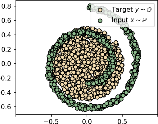
(a) Input, target measures.

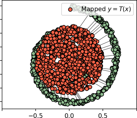
(b) IT map, $w\!=\!1$.

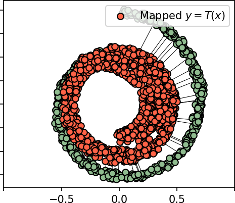
(c) IT map, $w\!=\!\nicefrac{{3}}{{2}}$.

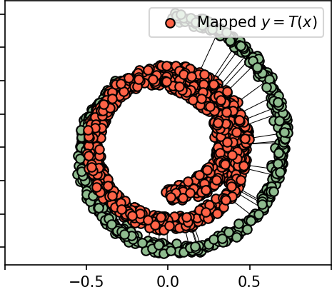
(d) IT map, $w\!=\!2$.

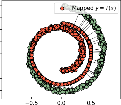
(e) IT map, $w\!=\!32$.

(f) Extremal transport map.

Figure 20: Incomplete Transport (IT) maps learned with $c(x,y)=\|x-y\|_{2}^{2}$ transport cost and ground-truth Extremal Transport (ET) map in ’Swiss2Ball experiment.

	$w=1$	$w=\nicefrac{{3}}{{2}}$	$w=2$	$w=32$
MSE($\hat{T},T^{*}$)	0.0136	0.0026	0.0009	7.98e-06

Table 8: MSE($\hat{T},T^{*}$) between learned IT maps $\hat{T}$ ($w\in\{1,\nicefrac{{3}}{{2}},2,32\}$) and ground-truth ET map $T^{*}$.

G.2 Solving Fake Solutions Issue with Weak Kernel Cost

As we discuss in Appendix A, saddle-point neural OT methods (including our IT algorithm) may suffer from fake solutions issue. As it is proved in [42], this issue can be eliminated by considering OT with the so-called weak kernel cost functions. In this section, we test the effect of using them in our IT algorithm. Specifically, we demonstrate the example where IT algorithm with the cost function $c(x,y)=\|x-y\|_{2}$ struggles from fake solutions, while IT with the same cost endowed with weak kernel regularization, i.e., kernel cost [42, Equation (16)] with parameters $\alpha=1,\gamma=0.4$, resolves the issue. Following [42], we consider stochastic version of IT map $T(x,z)$ using noise $z\sim\mathcal{N}(0,\mathcal{I})$ as an additional input.

We design the Ball2Circle example in 2D, where input $\mathbb{P}$ is a uniform distribution on a ball and target $\mathbb{Q}$ $-$ on a ring embracing the ball. The solution of ET problem is an internal circuit of a ring, see Fig. 21(a). We learn IT maps for $c(x,y)=\|x-y\|_{2}$, with ($\gamma=0.4)$ or without ($\gamma=0$) kernel regularization for weights $w\in\{1,2,32\}$.

(a) Input, target measures.

(b) IT map, ​$w\!=\!1$ (iter=7K)

(c) IT map, $w\!=\!\frac{3}{2}$ (iter=8K)

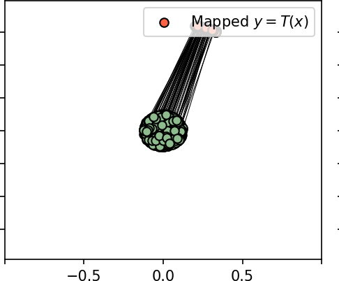
(d) IT map, $w\!=\!2$ (iter=7K)

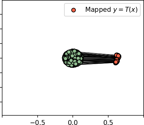
(e) IT map, $w\!=\!2$ (iter=8K).

(f) IT map, $w\!=\!32$

Figure 21: Incomplete Transport (IT) maps learned with $c(x,y)=\|x-y\|_{2}$ transport cost in ’Ball2Circle’ experiment. We observe that training is highly unstable for $w\in\{1,2\}$, see the solutions for nearby iterations of training - (b-c) and (d-e) respectively. Increase of the weight $w$ helps to improve the stability (f).

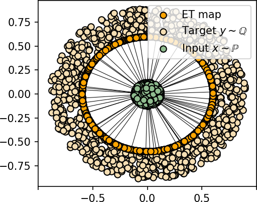
(a) Input, target measures and ET map.

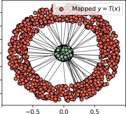
(b) IT map, $w\!=\!1$.

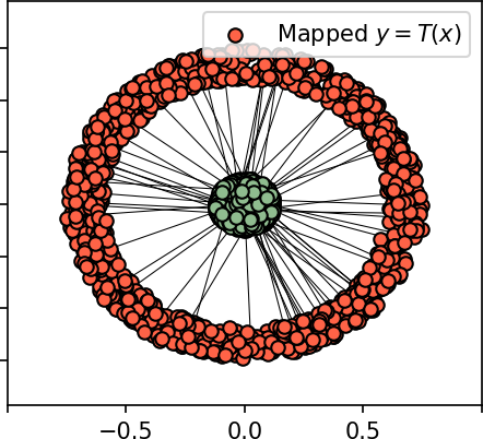
(c) IT map, $w\!=\!2$.

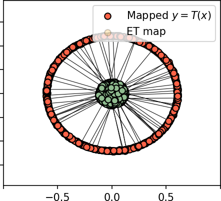
(d) IT map, $w\!=\!32$.

Figure 22: Incomplete transport (IT) maps learned with weak kernel cost in ’Ball2Circle’ experiment for a fixed noise $z$. Usage of the kernel regularization + stochastic map $T(x,z)$ helps to overcome instability issues for weights $w\in\{1,2\}$.

method / weight	$w=1$	$w=2$	$w=32$
w/o kernel regularization	-	-	0.0022
with kernel regularization	0.1377	0.0730	0.0495

Table 9: MSE($\hat{T},T^{*}$) between IT maps ($w\in\{1,2,32\}$) learned with $c(x,y)=\|x-y\|_{2}$ (with and without weak kernel regularization) and the ground-truth ET map. MSE for IT map learned with kernel regularization is larger (see $w=32$) than without the regularization since it introduces small bias to the optimization.

Discussion. We observe that without kernel regularization training of IT method is highly unstable (for $w\in\{1,2\}$), see Fig. 21(b)-21(d). Interestingly, with the increase of the weight $w$, the issue disappears and for $w=32$, IT map is close to the ground-truth ET one (Fig. 21(f)).

The usage of kernel regularization helps to improve stability of the method, see Fig. 22. However, while MSE between learned and ground-truth ET map drops with the increase of $w$, for $w=32$ it is bigger than that of learned IT maps without regularization. It is expected, since using regularizations usually leads to some bias in the solutions.

Thus, the example shows that (a) fake solutions may be a problem, (b) kernel regularization from [42] may help to deal with them. However, further studying this aspect is out of the scope of the paper.

G.3 Perceptual Cost

In this section, we show that the stated conclusions hold true for the transport costs other than $\ell^{2}$. For this purpose, we perform additional experiments using perceptual transport cost from [24]. We use the same hyperparameters as in our experiments with $\ell^{2}$ cost.

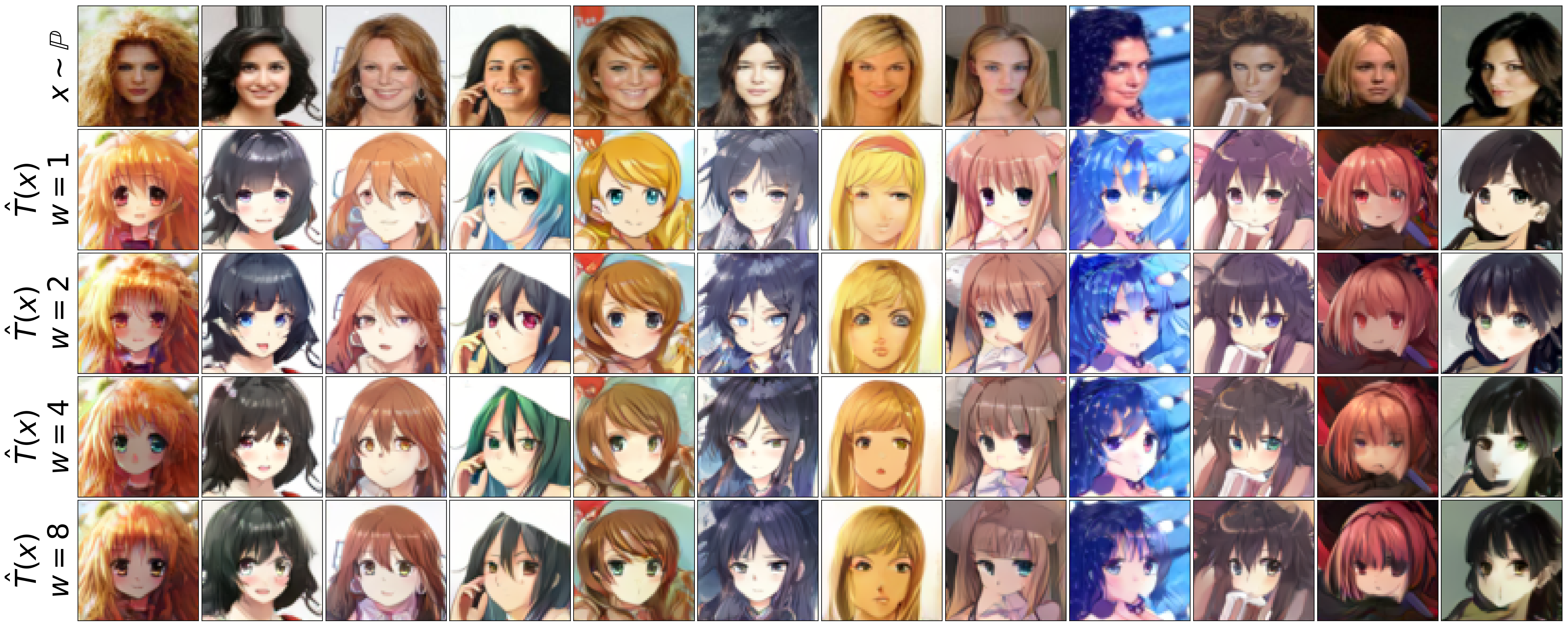
Figure 23: Celeba (female) $\rightarrow$ anime (64$\times$64 image size, perceptual cost).

Metrics	$w=1$	$w=2$	$w=4$	$w=8$
Test FID	9.21	12.98	17.24	22.08
Test perceptual cost	0.954	0.794	0.667	0.545
Test $\ell^{2}$ cost	0.303	0.209	0.153	0.103

Table 10: Test FID and $\ell^{2}$, perceptual transport costs of our IT maps (learned with perceptual transport cost).

Experimental results. Qualitative results show that that similarity of input images $x$ and the images $\hat{T}(x)$ translated by our IT method trained with perceptual cost grows with the increase of the parameter $w$, see Figure 23. In 10, we quantitatively verify these observations by showing that both perceptual and $\ell^{2}$ mean transport costs between input and translated images decrease with the increase of $w$. Interestingly, we see that IT trained with perceptual cost yields smaller FID than IT method trained with $\ell^{2}$ cost.

G.4 Bigger Weight Parameters

In this section, we present the results of IT method trained with $\ell^{2}$ cost and parameters $w=16,32$. We see that in contrast to CycleGAN which does not translate face images to anime images in case of big parameters $\lambda$, our IT method continues to translate faces to anime even for big parameters $w$. We quantify the obtained results in Table 11. As expected, mean transport costs are decreasing with the increase of $w$, while FID is slightly increasing. We present the qualitative results for additional weights in Figure 24.

Metrics	Main results				Additional results
	$w=1$	$w=2$	$w=4$	$w=8$	$w=16$	$w=32$
Test FID	14.65	20.79	22.18	22.84	24.86	28.28
Test $\ell^{2}$ cost	0.297	0.154	0.133	0.094	0.091	0.083

Table 11: Test FID and $\ell^{2}$ transport costs of our IT maps.

G.5 Additional Results for $\ell^{2}$ Cost

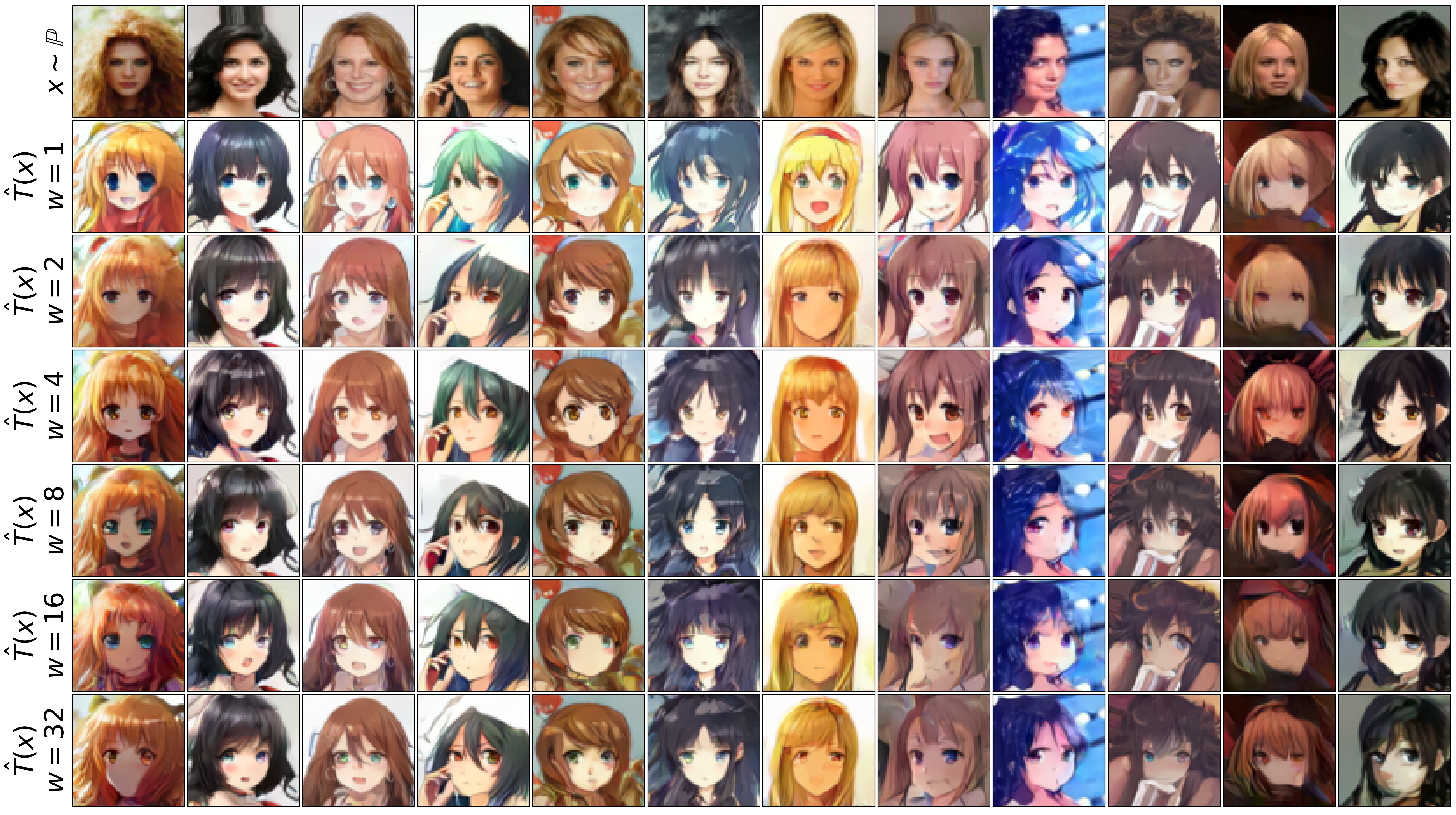
Figure 24: Celeba (female) $\rightarrow$ anime (64$\times$64).

Figure 25: Handbag $\rightarrow$ shoes (128$\times$128).

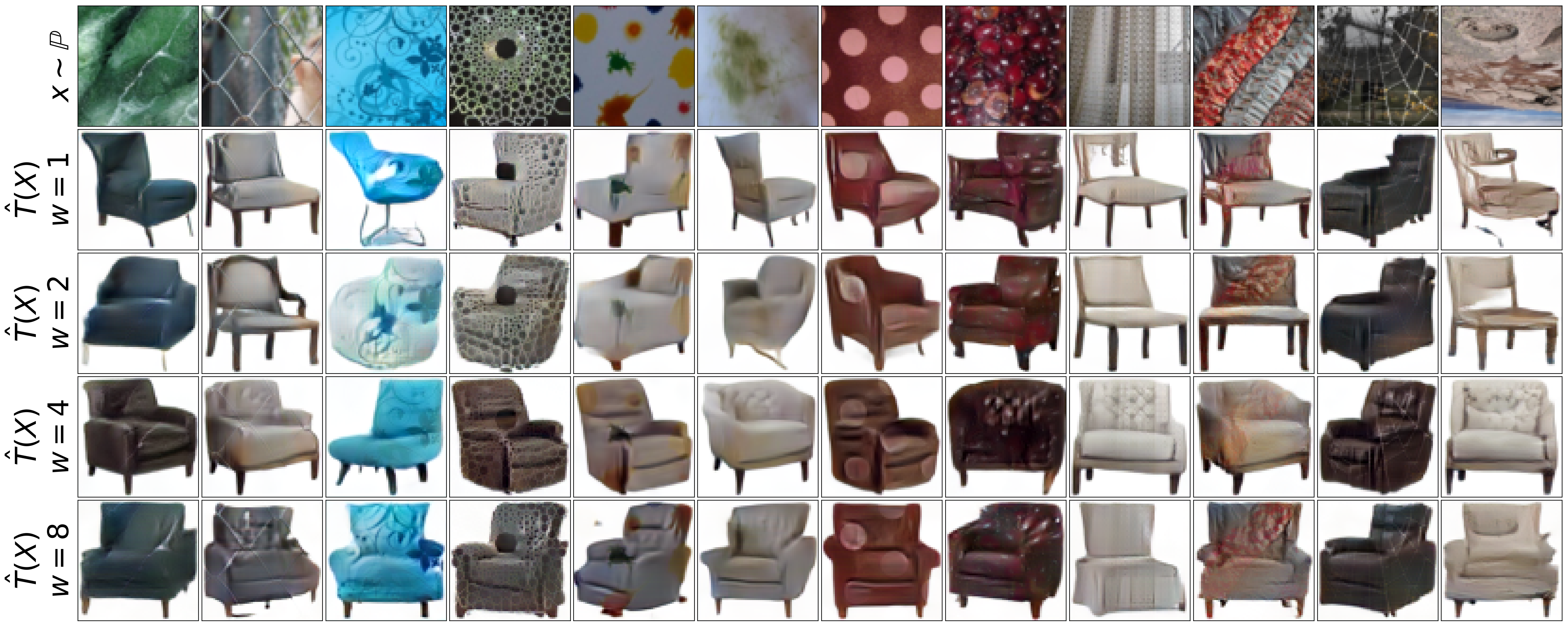
Figure 26: Textures $\rightarrow$ chairs (64$\times$64).

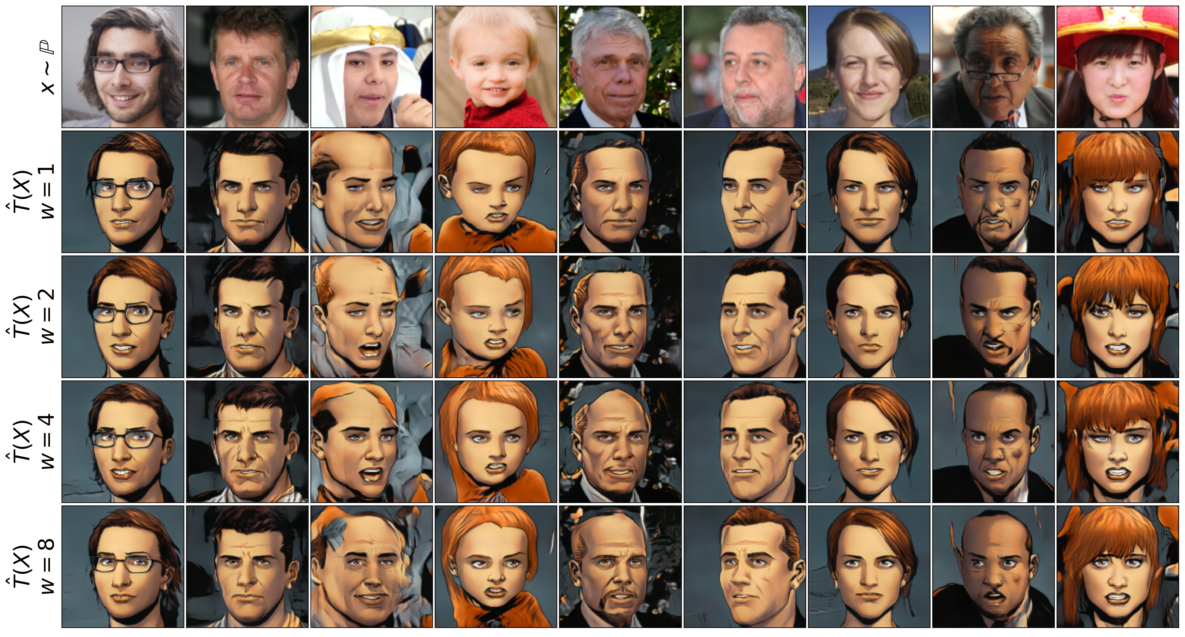
Figure 27: Ffhq $\rightarrow$ comics (128$\times$128).

References

- Aggarwal et al. [2018] D. Aggarwal, E. Valiyev, F. Sener, and A. Yao. Learning style compatibility for furniture. In German Conference on Pattern Recognition, pages 552–566. Springer, 2018.
- Aliprantis and Border [2006] C. D. Aliprantis and K. C. Border. Infinite dimensional analysis. Technical report, Springer, 2006.
- Alotaibi [2020] A. Alotaibi. Deep generative adversarial networks for image-to-image translation: A review. Symmetry, 12(10):1705, 2020.
- Arjovsky et al. [2017] M. Arjovsky, S. Chintala, and L. Bottou. Wasserstein generative adversarial networks. In International conference on machine learning, pages 214–223. PMLR, 2017.
- Asadulaev et al. [2022] A. Asadulaev, A. Korotin, V. Egiazarian, and E. Burnaev. Neural optimal transport with general cost functionals. arXiv preprint arXiv:2205.15403, 2022.
- Babenko et al. [2014] A. Babenko, A. Slesarev, A. Chigorin, and V. Lempitsky. Neural codes for image retrieval. In European conference on computer vision, pages 584–599. Springer, 2014.
- Balaji et al. [2020] Y. Balaji, R. Chellappa, and S. Feizi. Robust optimal transport with applications in generative modeling and domain adaptation. Advances in Neural Information Processing Systems, 33:12934–12944, 2020.
- Bińkowski et al. [2018] M. Bińkowski, D. J. Sutherland, M. Arbel, and A. Gretton. Demystifying mmd gans. In International Conference on Learning Representations, 2018.
- Brown et al. [2020] T. Brown, B. Mann, N. Ryder, M. Subbiah, J. D. Kaplan, P. Dhariwal, A. Neelakantan, P. Shyam, G. Sastry, A. Askell, et al. Language models are few-shot learners. Advances in neural information processing systems, 33:1877–1901, 2020.
- Caffarelli and McCann [2010] L. A. Caffarelli and R. J. McCann. Free boundaries in optimal transport and monge-ampere obstacle problems. Annals of mathematics, pages 673–730, 2010.
- Chapel et al. [2020] L. Chapel, M. Z. Alaya, and G. Gasso. Partial optimal tranport with applications on positive-unlabeled learning. Advances in Neural Information Processing Systems, 33:2903–2913, 2020.
- Chen et al. [2022] H. Chen, X. He, L. Qing, Y. Wu, C. Ren, R. E. Sheriff, and C. Zhu. Real-world single image super-resolution: A brief review. Information Fusion, 79:124–145, 2022.
- Chen and Jia [2021] X. Chen and C. Jia. An overview of image-to-image translation using generative adversarial networks. In International Conference on Pattern Recognition, pages 366–380. Springer, 2021.
- Chizat [2017] L. Chizat. Unbalanced optimal transport: Models, numerical methods, applications. PhD thesis, Université Paris sciences et lettres, 2017.
- Choi et al. [2020] Y. Choi, Y. Uh, J. Yoo, and J.-W. Ha. Stargan v2: Diverse image synthesis for multiple domains. In Proceedings of the IEEE/CVF conference on computer vision and pattern recognition, pages 8188–8197, 2020.
- Cimpoi et al. [2014] M. Cimpoi, S. Maji, I. Kokkinos, S. Mohamed, , and A. Vedaldi. Describing textures in the wild. In Proceedings of the IEEE Conf. on Computer Vision and Pattern Recognition (CVPR), 2014.
- Daniels et al. [2021] M. Daniels, T. Maunu, and P. Hand. Score-based generative neural networks for large-scale optimal transport. Advances in neural information processing systems, 34:12955–12965, 2021.
- de Bézenac et al. [2021] E. de Bézenac, I. Ayed, and P. Gallinari. Cyclegan through the lens of (dynamical) optimal transport. In Machine Learning and Knowledge Discovery in Databases. Research Track: European Conference, ECML PKDD 2021, Bilbao, Spain, September 13–17, 2021, Proceedings, Part II 21, pages 132–147. Springer, 2021.
- Eyring et al. [2022] L. V. Eyring, D. Klein, G. Palla, S. Becker, P. Weiler, N. Kilbertus, and F. Theis. Modeling single-cell dynamics using unbalanced parameterized monge maps. bioRxiv, 2022.
- Fan et al. [2023] J. Fan, S. Liu, S. Ma, H.-M. Zhou, and Y. Chen. Neural monge map estimation and its applications. Transactions on Machine Learning Research, 2023. ISSN 2835-8856. URL https://openreview.net/forum?id=2mZSlQscj3. Featured Certification.
- Fefferman et al. [2016] C. Fefferman, S. Mitter, and H. Narayanan. Testing the manifold hypothesis. Journal of the American Mathematical Society, 29(4):983–1049, 2016.
- Figalli [2010] A. Figalli. The optimal partial transport problem. Archive for rational mechanics and analysis, 195(2):533–560, 2010.
- Folland [1999] G. B. Folland. Real analysis: modern techniques and their applications, volume 40. John Wiley & Sons, 1999.
- Gazdieva et al. [2022] M. Gazdieva, L. Rout, A. Korotin, A. Kravchenko, A. Filippov, and E. Burnaev. An optimal transport perspective on unpaired image super-resolution. arXiv preprint arXiv:2202.01116, 2022.
- Genevay et al. [2016] A. Genevay, M. Cuturi, G. Peyré, and F. Bach. Stochastic optimization for large-scale optimal transport. In Advances in neural information processing systems, pages 3440–3448, 2016.
- Genevay et al. [2018] A. Genevay, G. Peyré, and M. Cuturi. Learning generative models with sinkhorn divergences. In International Conference on Artificial Intelligence and Statistics, pages 1608–1617. PMLR, 2018.
- Goodfellow et al. [2014] I. Goodfellow, J. Pouget-Abadie, M. Mirza, B. Xu, D. Warde-Farley, S. Ozair, A. Courville, and Y. Bengio. Generative adversarial nets. In Advances in neural information processing systems, pages 2672–2680, 2014.
- Gulrajani et al. [2017] I. Gulrajani, F. Ahmed, M. Arjovsky, V. Dumoulin, and A. C. Courville. Improved training of Wasserstein GANs. In Advances in Neural Information Processing Systems, pages 5767–5777, 2017.
- Gushchin et al. [2023] N. Gushchin, A. Kolesov, A. Korotin, D. Vetrov, and E. Burnaev. Entropic neural optimal transport via diffusion processes. In Advances in Neural Information Processing Systems, 2023.
- He et al. [2016] K. He, X. Zhang, S. Ren, and J. Sun. Deep residual learning for image recognition. In Proceedings of the IEEE conference on computer vision and pattern recognition, pages 770–778, 2016.
- Henry-Labordere [2019] P. Henry-Labordere. (martingale) optimal transport and anomaly detection with neural networks: A primal-dual algorithm. arXiv preprint arXiv:1904.04546, 2019.
- Heusel et al. [2017] M. Heusel, H. Ramsauer, T. Unterthiner, B. Nessler, and S. Hochreiter. GANs trained by a two time-scale update rule converge to a local nash equilibrium. In Advances in neural information processing systems, pages 6626–6637, 2017.
- Huang et al. [2018] X. Huang, M.-Y. Liu, S. Belongie, and J. Kautz. Multimodal unsupervised image-to-image translation. In Proceedings of the European conference on computer vision (ECCV), pages 172–189, 2018.
- Jing et al. [2019] Y. Jing, Y. Yang, Z. Feng, J. Ye, Y. Yu, and M. Song. Neural style transfer: A review. IEEE transactions on visualization and computer graphics, 26(11):3365–3385, 2019.
- Johnson et al. [2019] J. Johnson, M. Douze, and H. Jégou. Billion-scale similarity search with gpus. IEEE Transactions on Big Data, 7(3):535–547, 2019.
- Karras et al. [2019] T. Karras, S. Laine, and T. Aila. A style-based generator architecture for generative adversarial networks. In Proceedings of the IEEE/CVF conference on computer vision and pattern recognition, pages 4401–4410, 2019.
- Karush [2014] W. Karush. Minima of functions of several variables with inequalities as side conditions. In Traces and Emergence of Nonlinear Programming, pages 217–245. Springer, 2014.
- Kingma and Ba [2014] D. P. Kingma and J. Ba. Adam: A method for stochastic optimization. arXiv preprint arXiv:1412.6980, 2014.
- Korotin et al. [2021a] A. Korotin, V. Egiazarian, A. Asadulaev, A. Safin, and E. Burnaev. Wasserstein-2 generative networks. In International Conference on Learning Representations, 2021a. URL https://openreview.net/forum?id=bEoxzW_EXsa.
- Korotin et al. [2021b] A. Korotin, L. Li, A. Genevay, J. M. Solomon, A. Filippov, and E. Burnaev. Do neural optimal transport solvers work? a continuous wasserstein-2 benchmark. Advances in Neural Information Processing Systems, 34:14593–14605, 2021b.
- Korotin et al. [2022] A. Korotin, A. Kolesov, and E. Burnaev. Kantorovich strikes back! wasserstein gans are not optimal transport? In Thirty-sixth Conference on Neural Information Processing Systems Datasets and Benchmarks Track, 2022.
- Korotin et al. [2023a] A. Korotin, D. Selikhanovych, and E. Burnaev. Kernel neural optimal transport. In International Conference on Learning Representations, 2023a. URL https://openreview.net/forum?id=Zuc_MHtUma4.
- Korotin et al. [2023b] A. Korotin, D. Selikhanovych, and E. Burnaev. Neural optimal transport. In International Conference on Learning Representations, 2023b. URL https://openreview.net/forum?id=d8CBRlWNkqH.
- Li et al. [2023] Z. Li, Y. Xu, N. Zhao, Y. Zhou, Y. Liu, D. Lin, and S. He. Parsing-conditioned anime translation: A new dataset and method. ACM Transactions on Graphics, 42(3):1–14, 2023.
- Liu et al. [2019] H. Liu, X. Gu, and D. Samaras. Wasserstein GAN with quadratic transport cost. In Proceedings of the IEEE International Conference on Computer Vision, pages 4832–4841, 2019.
- Liu et al. [2015] Z. Liu, P. Luo, X. Wang, and X. Tang. Deep learning face attributes in the wild. In Proceedings of International Conference on Computer Vision (ICCV), December 2015.
- Lübeck et al. [2022] F. Lübeck, C. Bunne, G. Gut, J. S. del Castillo, L. Pelkmans, and D. Alvarez-Melis. Neural unbalanced optimal transport via cycle-consistent semi-couplings. arXiv preprint arXiv:2209.15621, 2022.
- Lucic et al. [2018] M. Lucic, K. Kurach, M. Michalski, S. Gelly, and O. Bousquet. Are GANs created equal? a large-scale study. In Advances in neural information processing systems, pages 700–709, 2018.
- Makkuva et al. [2020] A. Makkuva, A. Taghvaei, S. Oh, and J. Lee. Optimal transport mapping via input convex neural networks. In International Conference on Machine Learning, pages 6672–6681. PMLR, 2020.
- Malkov and Yashunin [2018] Y. A. Malkov and D. A. Yashunin. Efficient and robust approximate nearest neighbor search using hierarchical navigable small world graphs. IEEE transactions on pattern analysis and machine intelligence, 42(4):824–836, 2018.
- Mathur et al. [2019] A. Mathur, A. Isopoussu, F. Kawsar, N. Berthouze, and N. D. Lane. Mic2mic: using cycle-consistent generative adversarial networks to overcome microphone variability in speech systems. In Proceedings of the 18th international conference on information processing in sensor networks, pages 169–180, 2019.
- Mukherjee et al. [2021] D. Mukherjee, A. Guha, J. M. Solomon, Y. Sun, and M. Yurochkin. Outlier-robust optimal transport. In International Conference on Machine Learning, pages 7850–7860. PMLR, 2021.
- Nhan Dam et al. [2019] Q. H. Nhan Dam, T. Le, T. D. Nguyen, H. Bui, and D. Phung. Threeplayer Wasserstein GAN via amortised duality. In Proc. of the 28th Int. Joint Conf. on Artificial Intelligence (IJCAI), 2019.
- Nietert et al. [2022] S. Nietert, Z. Goldfeld, and R. Cummings. Outlier-robust optimal transport: Duality, structure, and statistical analysis. In International Conference on Artificial Intelligence and Statistics, pages 11691–11719. PMLR, 2022.
- Pang et al. [2021] Y. Pang, J. Lin, T. Qin, and Z. Chen. Image-to-image translation: Methods and applications. IEEE Transactions on Multimedia, 2021.
- Peyré et al. [2019] G. Peyré, M. Cuturi, et al. Computational optimal transport. Foundations and Trends® in Machine Learning, 11(5-6):355–607, 2019.
- Radford et al. [2021] A. Radford, J. W. Kim, C. Hallacy, A. Ramesh, G. Goh, S. Agarwal, G. Sastry, A. Askell, P. Mishkin, J. Clark, et al. Learning transferable visual models from natural language supervision. In International Conference on Machine Learning, pages 8748–8763. PMLR, 2021.
- Ramesh et al. [2022] A. Ramesh, P. Dhariwal, A. Nichol, C. Chu, and M. Chen. Hierarchical text-conditional image generation with clip latents. arXiv preprint arXiv:2204.06125, 2022.
- Rockafellar [1976] R. T. Rockafellar. Integral functionals, normal integrands and measurable selections. In Nonlinear operators and the calculus of variations, pages 157–207. Springer, 1976.
- Ronneberger et al. [2015] O. Ronneberger, P. Fischer, and T. Brox. U-net: Convolutional networks for biomedical image segmentation. In International Conference on Medical image computing and computer-assisted intervention, pages 234–241. Springer, 2015.
- Rout et al. [2022] L. Rout, A. Korotin, and E. Burnaev. Generative modeling with optimal transport maps. In International Conference on Learning Representations, 2022.
- Santambrogio [2015] F. Santambrogio. Optimal transport for applied mathematicians. Birkäuser, NY, 55(58-63):94, 2015.
- Seguy et al. [2018] V. Seguy, B. B. Damodaran, R. Flamary, N. Courty, A. Rolet, and M. Blondel. Large scale optimal transport and mapping estimation. In International Conference on Learning Representations, 2018.
- Terkelsen [1972] F. Terkelsen. Some minimax theorems. Mathematica Scandinavica, 31(2):405–413, 1972.
- Villani [2008] C. Villani. Optimal transport: old and new, volume 338. Springer Science & Business Media, 2008.
- Yang and Uhler [2018] K. D. Yang and C. Uhler. Scalable unbalanced optimal transport using generative adversarial networks. In International Conference on Learning Representations, 2018.
- Yu and Grauman [2014] A. Yu and K. Grauman. Fine-grained visual comparisons with local learning. In Proceedings of the IEEE Conference on Computer Vision and Pattern Recognition, pages 192–199, 2014.
- Yu et al. [2015] F. Yu, A. Seff, Y. Zhang, S. Song, T. Funkhouser, and J. Xiao. Lsun: Construction of a large-scale image dataset using deep learning with humans in the loop. arXiv preprint arXiv:1506.03365, 2015.
- Yuan et al. [2018] Y. Yuan, S. Liu, J. Zhang, Y. bing Zhang, C. Dong, and L. Lin. Unsupervised image super-resolution using cycle-in-cycle generative adversarial networks. 2018 IEEE/CVF Conference on Computer Vision and Pattern Recognition Workshops (CVPRW), pages 814–81409, 2018.
- Zhang et al. [2018] R. Zhang, P. Isola, A. A. Efros, E. Shechtman, and O. Wang. The unreasonable effectiveness of deep features as a perceptual metric. In CVPR, 2018.
- Zhang et al. [2022] X. Zhang, D. Zhai, T. Li, Y. Zhou, and Y. Lin. Image inpainting based on deep learning: A review. Information Fusion, 2022.
- Zhu et al. [2017] J.-Y. Zhu, T. Park, P. Isola, and A. A. Efros. Unpaired image-to-image translation using cycle-consistent adversarial networks. In Proceedings of the IEEE international conference on computer vision, pages 2223–2232, 2017.