Does Deconfined Quantum Phase Transition Have to Keep Lorentz Symmetry?
Two Velocities of Spinon and String

Abstract

Lorentz symmetry is commonly assumed to be an intrinsic requirement of the (2+1)d deconfined quantum phase transition (DQPT), and the conformal field theory (CFT) can be utilized. The dynamics of DQPT in the Kagome lattice are explored by using a combination of large-scale quantum Monte Carlo simulations and stochastic analytic continuation. In the valence-bonded solid phase, the fragmentation of a nearly flat band with a finite energy gap is observed around the K point. At the deconfined quantum critical point, besides the linear dispersion at the $\Gamma$ point, another one is found at the K point. Counterintuitively, these two gapless modes take different speeds equal to 0.319(8) and 0.101(9), indicating the absence of Lorentz symmetry. After carefully inspecting the snapshot of the simulation, we discovered the fast mode at $\Gamma$ point corresponding to the deconfinement of spinons (fractional charges), and the slow mode at K point is related to the quantum string ( generalized symmetry). Our work will extend the understanding of phase transition, and intrigue the field of topological quantum field theory.

Introduction—The Ginzburg-Landau theory makes a great achievement on comprehension of the phase transitions. However, the deconfined quantum phase transition (DQPT) is a prototypical counter example, e.g. the Néel phase can undergo a continuous transition to the valence bond solid (VBS) Senthil et al. (2004a, b); Sandvik (2007, 2007); Nahum et al. (2015); Wang et al. (2017); Qin et al. (2017); Liu et al. (2019); Zhang et al. (2018).At the deconfined quantum critical point (DQCP), the quasi-long range order with power-law decaying accompanies the fractional excitations and emergent gauge fields, which is reminiscent of the quantum spin liquid Broholm et al. (2020). It is a common belief that the DQCP preserves the Lorentz symmetry and the conformal field theory (CFT) still works Wang et al. (2017).

Among the possible candidates, the DQPT in the Kagome lattice appears to be special Damle and Senthil (2006); Isakov et al. (2006); Zhang and Eggert (2013); Zhang et al. (2018). The interplay between geometric frustration and strong interactions leads to local constraints. Thus, same as the quantum spin ice Savary and Balents (2012); Gingras and McClarty (2014); Xiong et al. (2021), the relation between the lattice Hamiltonian (UV) and the effective gauge theory model (IR) is not obscure Zhang et al. (2018). The topological defects can be directly observed from snapshots of quantum Monte Carlo (QMC) simulations Zhang and Eggert (2013), such as spinons (fractional charges) and quantum string excitations preserving generalized symmetry McGreevy (2022). Meanwhile, the correlation of the spinons can also be calculated, and the scaling behavior meets the prediction of CFT Zhang et al. (2018). However, recent research on the disorder operators in some DQCP candidates conflicts with the unitary CFT Wang et al. (2022); Liu et al. (2022); Ma and Wang (2020).

Recently, the rapid development of the stochastic analytic continuation (SAC) method provides an ideal detector to analyze the dynamics of the excitations including the topological ones Shao and Sandvik (2023); Shao et al. (2017); Ma et al. (2018); Zhou et al. (2022); Xiong et al. (2021). Therefore, it is expected that the roles of the fractional charge and quantum strings playing on the DQPT can be figured out from the dynamic spectra Zhou et al. (2022). Meanwhile, the Lorentz symmetry can also be checked.

In this manuscript, we study the dynamics of the DQPT between VBS and superfluid (SF) phases in the Kagome lattice with a large-scale QMC method. As shown in Fig. 1 (a), two types of linear dispersion are observed at $\Gamma$ and K points, respectively. The large deviation between their speeds is verified after careful finite-size scaling analysis, and it indicates the Lorentz symmetry is non-existent at the DQCP. Finally, we map the snapshot of the real space configuration at the DQCP to the representation of the lattice gauge fields. Then, the different speeds can be interpreted by the dispersion of the spinons and the vibrations of the quantum strings.

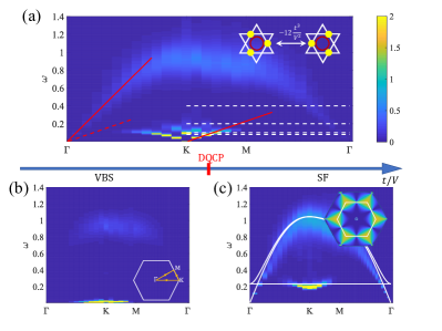
Figure 1: The dynamic spectra of (a) DQCP at $t/V=0.1302$, (b) VBS phase at $t/V=0.08$, and (c) SF phase at $t/V=0.20$ calculated with QMC simulation. The system size is $L=36$ with inverse temperature $\beta=600$. The inset of (a) presents the third-order ring exchange, the red solid lines show the fitting speeds at $\Gamma$ and K point (red dash line for comparison), and the white dash lines highlight the parameter regions in Fig.2. The scanning path $\Gamma$-K-M-$\Gamma$ is depicted in the inset of (b). The solid white lines in (c) are energy dispersion calculated by LSWT. The inset of (c) is DSF calculated by LSWT with constant energy cut close to the flat band.

Model—We consider the extended hard-core Bose-Hubbard Hamiltonian Damle and Senthil (2006); Isakov et al. (2006); Zhang and Eggert (2013); Zhang et al. (2018) written as

$$H=-t\sum_{\langle i,j\rangle}(b^{\dagger}_{i}b_{j}+h.c.)+V\sum_{\langle i,j\rangle}n_{i}n_{j},$$ (1)

where $t\geq 0$ and $V\geq 0$ denote the hopping and repulsive interaction between nearest-neighbor sites, and $b^{\dagger}_{i}$ ($b_{i}$) is creation (annihilation) operator of the hard-core boson which could be used for describing the Rydberg-dressed atom in the optical lattice Hollerith et al. (2022). It is equivalent to the spin half XXZ model after implementing the mapping $b^{\dagger}_{i}\rightarrow S^{+}_{i}$, $b_{i}\rightarrow S^{-}_{i}$ and $n_{i}\rightarrow S_{i}^{z}+1/2$ Zhang et al. (2011). Because the DQPT happens at average density equal to $1/3$, the numerical simulation is implemented in the canonical ensemble and the chemical potential (or magnetic field) is not included in Eq.(1) Zhang et al. (2018). Here, we choose $V$ as the energy unit.

In order to minimize the ground state energy, the repulsive interaction imposes a strong local constrain — each triangle of the Kagome lattice can be occupied with only one particle (e.g. or ). It is named as triangle rule, similar as ice rule in the quantum spin ice Savary and Balents (2012). Because the configuration satisfying the triangle rule is not unique, the ground state is disordered with macroscopic degeneracy Pauling (1935). However, in the strong coupling region $t/V\ll 1$, a third-order perturbative interaction $H_{\textrm{ring}}=-\frac{12t^{3}}{V^{2}}\sum(|{\leavevmode\hbox to10.44pt{\vbox to10.16pt{\text{[drawing]}}}}\rangle\langle\leavevmode\hbox to10.44pt{\vbox to10.16pt{\text{[drawing]}}}|+h.c.)$ can exchange the configuration in each hexagon without breaking the triangle rule (see inset of Fig.1(a)). This effective ring exchange interaction can lift the degeneracy so that the system enters into the VBS phase which breaks the translational symmetry. Although some spinons (e.g. or ) can still be excited due to the quantum fluctuation, the large energy gap $V$ makes them be confined.

In the weak coupling region $t\gg V$, the large hopping process makes the bosons break the U(1) symmetry so that the system enters into the SF phase. In the spin language, it is equivalent to the ferromagnetic XY phase, and the linear spin wave theory (LSWT) is a quite suitable method. As shown in Fig.1(c) along the selected path $\Gamma$-K-M-$\Gamma$ in the Brillouin zone, there are three branches: the lowest gapless branch at $\Gamma$ point with the linear dispersion corresponds to the Goldstone mode; the flat-band branch results from the lattice geometry Pudleiner and Mielke (2015); the highest branch meets the flat band at $\Gamma$ point.

At the critical point, the interplay between the spinons (gauge charge) and the emergent dynamical U(1) gauge field causes the deconfined criticality. Several exotic phenomena can be found, such as the drift of the superfluid density, large anomalous critical exponent, emergent symmetries and so on Zhang et al. (2018). It is a common belief that this DQPT can be described by the easy plane NCCP¹ theory Senthil et al. (2004a, b) which means the emergent Lorentz symmetry is kept and the CFT can be used.

Spectra of phases—The numerical method adopted is the stochastic cluster series expansion with parallel tempering Sengupta et al. (2002) which can greatly overcome the non-ergodic problem. We choose the periodical boundary condition (PBC) with largest system size reaches $N=36\times 36\times 3=3888$ spins. Meanwhile, in order to suppress the influence of the thermal fluctuation, the temperature is set to be $T=1/\beta=\frac{6V}{100L}$ which is even lower than our previous work Zhang et al. (2018). Here, we focus on the dynamical structure factor (DSF) $S^{zz}({\textbf{k}},\omega)$, and it can be extracted from the imaginary time correlation function $S^{zz}(\textbf{r},\tau)=\langle S^{z}(\textbf{0},0)S^{z}(\textbf{r},\tau)\rangle$ by implementing the SAC method Shao and Sandvik (2023); Shao et al. (2017); Zhou et al. (2022). The QMC samples is more than five million, so that the high-quality spectra can be obtained.

In the VBS phase, two branches can be observed in Fig.1 (b). The lower branch stays on a very low energy scale and is nearly flat with a tiny gap. The flat band is usually related to the lattice geometry, and it reflects the localization of the particles caused by the effective ring exchange interaction Pudleiner and Mielke (2015). Similar to the checkerboard lattice Xiong et al. (2021), it corresponds to the excitation from triplet ground state $\frac{1}{\sqrt{2}}(|{\leavevmode\hbox to10.44pt{\vbox to10.16pt{\text{[drawing]}}}}\rangle+|\leavevmode\hbox to10.44pt{\vbox to10.16pt{\text{[drawing]}}}\rangle)$ to the singlet state $\frac{1}{\sqrt{2}}(|{\leavevmode\hbox to10.44pt{\vbox to10.16pt{\text{[drawing]}}}}\rangle-|\leavevmode\hbox to10.44pt{\vbox to10.16pt{\text{[drawing]}}}\rangle)$, so its energy scale is $\sim\frac{12t^{3}}{V^{2}}$. Meanwhile, we can find the flat band only appears in a certain region. This fragmentation hints at the existence of some “selection rule” Xiong et al. (2021). On the other hand, the higher branch has a large energy gap $\sim V$, and it is relevant to the spinon separation due to the local quantum fluctuation.

In the SF phase, the numerical spectrum in Fig.1(c) also shows two branches. The energy scale of flat band branch increases a lot, and the fragmentation remains. From the LSWT calculation of DSF at flat band (inset of Fig.1(c)), we can find no intensity along the path M-$\Gamma$ which is consistent with the numerical results. We think this fragmentation should also result from some “selection rule” due to the lattice symmetries Xiong et al. (2021). On the other hand, the higher branch is the gapless Goldstone mode.

Spectra of DQCP—The VBS and SF phases break different symmetries but can still undergo a continuous phase transition at the DQCP. As shown in Fig.1 (a) at DQCP, the higher branch (named $\Gamma$-branch) is gapless at $\Gamma$ point and has a similar shape as the SF phase but with lower intensity. Deformed from the Goldstone mode in the SF phase, the $\Gamma$-branch becomes more continuous in a high energy scale, and it indicates the emergence of the fractional charges at DQCP. Notice that, here we do not choose the logarithmic scale in the $\omega$ axis and do not make the interpolation of the original SAC data, so the continuum may appear less obvious.

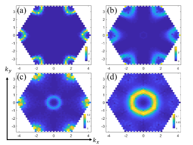
Figure 2: The tomographic slices of DSF at DQCP calculated by QMC-SAC with fixed $\omega$ equal to (a-d) 0.08, 0.10, 0.20, and 0.40. The system size is $L=36$ with inverse temperature $\beta=600$. The colored region is the first Brillouin zone. Because the DSF only can have a non-zero value at the reciprocal lattice site in PBC, the color in each tiny hexagon marks the value of DSF at k of the center of hexagon.

The lower branch (named K-branch) is strongly changed and no longer flat, but the “selection rule” still holds. Another gapless linear mode appears at K points where the order parameter of the VBS phase stays. Most strikingly, it has different speed with $\Gamma$-branch, and can be clearly distinguished even with the naked eye. The dispersion of $\Gamma$-branch is faster than K-branch. This implies that the low-energy effective theory cannot be invariant under Lorentz transformations with one velocity. Then the breakdown of Lorentz symmetry immediately points to the inapplicability of the CFT at the DQCP. To obtain more details at the DQCP, we calculate the DSF over the entire first Brillouin zone. Then, the tomographic slices with fixed $\omega$ can be got and used for scanning the dynamics at DQCP.

The K-branch has a higher intensity at low $\omega$ in comparison with $\Gamma$-branch. In Fig.2(a), it is nearly isotropic around the K point. However, while increasing the energy scale, it becomes anisotropic (Fig.2(b)) and the U(1) symmetry is broken down to Z₃. Actually, in previous work Zhang et al. (2018); Pujari et al. (2013), the histogram of order parameter at DQCP does not exhibit perfect emergent U(1) symmetry expected in theory. According to the NCCP¹ theory, the anisotropy may result from the three-fold monopoles which are highly closed to marginal Pujari et al. (2013); Block et al. (2013). From the dynamic spectra, we think that the possible emergent U(1) symmetry of VBS order parameter stays at a very low energy scale $\sim 0.09V$, so the elimination of the anisotropy requires an extremely low temperature. At high $\omega$ in Fig.2 (c-d), the DSF around the K point becomes messy or weaker, and no information of K-branch can be further extracted. While increasing $\omega$, the $\Gamma$-branch becomes more clear along with the weakening of the K-branch. In contrast, the $\Gamma$-branch is more isotropic.

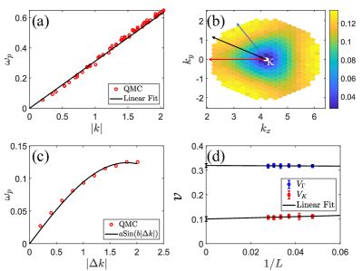
Figure 3: The position of the peak $\omega_{p}(\textbf{k})$ of (a) the $\Gamma$-branch, (b) the K-branch, and (c) along angular bisector direction (black arrow in (b)). The speed of K-branch is obtained by fitting the data along angular bisector direction between the $\Gamma$-K direction (blue arrow) and M-K direction (red arrow). The system size is $L=36$ with inverse temperature $\beta=600$. (d) The finite size scaling analysis of two speeds is implemented with linear fitting the data at $L=21:3:36$ and $\beta=\frac{100L}{6V}$. The error bars on the $v$-axis show the fitted values for the two velocities in the thermodynamic limit.

The velocities of different modes can be extracted from the position of the peak $\omega_{p}(\textbf{k})$ at different momentum k. Here, to avoid introducing an additional error of unnecessary fitting, we take $\omega_{p}(\textbf{k})$ at which the DSF reaches its local maximum at fixed k. The Fig.3 (a) plots the relation between $\omega_{p}(\textbf{k})$ and the magnitude of k. We can find the $\omega_{p}(\textbf{k})$ depends less on the angle of k, and it firmly demonstrates the isotropy of the $\Gamma$-branch. Meanwhile, the numerical data of $\omega_{p}(\textbf{k})$ matches well with the linear fitting result, and it indicates the constant speed of the linear dispersion at $\Gamma$ point, $V_{\Gamma}=0.317(8)$ at $L=36$.

In comparison, the dispersion of the K-branch is more complicated. In Fig.3(b), the DSF around the K point presents the clear feature of the anisotropy. The fastest velocity is along the $\Gamma$-K direction (blue arrow), and the slowest one is along M-K direction (red arrow). However, both of them have few data points, e.g., five at $L=36$. In comparison, there are more data points along the angular bisector direction (black arrow), e.g. ten at $L=36$. In order to obtain the speed of K-branch $V_{K}$ with high accuracy, we select the angular bisector direction for fitting. Different from the $\Gamma$-branch, the higher energy part of the K-branch exhibits a strong deviation from the linearity. Actually, as shown in Fig.3(c), we find the sine function $\omega_{p}(\Delta\textbf{k})=a\sin{b|\Delta\textbf{k}|}$ ($\Delta\textbf{k}=\textbf{k}-(4\pi/3,0)$) shows better goodness of fitting than the linear fitting. Then, the speed of K-branch can be calculated by $V_{K}=|ab|$. Furthermore, we want to emphasize that the anisotropy does not bring serious deviation, like the speeds in fast, slow, and angular bisector direction at $L=36$ are 0.114(15), 0.103(21), and 0.107(8), respectively.

The strong difference between two speeds of $\Gamma$-branch and K-branch indicates they originate from different physical mechanisms. First, however, we have to implement a finite-size scaling analysis to exclude possible normalization prefactors. In Fig.3 (d), $V_{\Gamma}$ and $V_{K}$ at different system size are shown. We can find that the finite size effects are very weak, and the numerical data matches well with the linear fitting results. Finally, in the thermodynamic limit, we estimate the speed of $\Gamma$-branch is 0.319(8), and the speed of K-branch is 0.101(9). As mentioned before, it means there are two types of gapless quasi-particle excitation with completely different speeds, therefore the Lorentz symmetry can not emerge and the low-energy physics of the DQPT should be rethought.

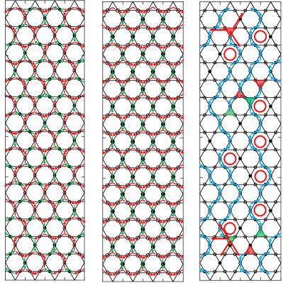
Figure 4: A snapshot of a typical configuration during a Monte Carlo run is shown in the left panel. The middle panel presents the reference vacuum state. The red (green) arrows mark the “electric field” with a value -1/3 (2/3). After subtracting the vacuum state, the open string (“electric field line”) linked with the spinon (“electric charge”) is shown in the right panel. The red (green) triangle labels the spinon taking negative (positive) charge one. The red arrows in the right panel show the possible directions of the spinon motion. The blue arrows mark the “electric field” with value one. The red cycles label the hexagon where the ring exchange term can deform the string.

Phenomenological Analysis—At DQCP, it is worth introducing the lattice gauge field mapping for understanding the physical mechanism of topological excitations, especially the spinon (gauge charge) and string (field line) Zhang and Eggert (2013); Zhang et al. (2018). As demonstrated in the left panel of Fig.4, the hard-core boson can be mapped into the “electric field” defined at the bisector of corner-shared triangle via the relation $E_{ll^{\prime}}=n_{i}-1/3$, where $l$ locates at the triangle center and labels the site of the dual honeycomb lattice. The gauge charges sit on the sites of dual lattice and can be calculated by summing all field lines around one triangle via the “Gauss law”. Meanwhile, the configurations satisfying the triangle rule are the pure gauge field, and its dynamics are mainly controlled by the ring exchange term which acts as the “magnetic field” Savary and Balents (2012); Xiong et al. (2021); Zhang et al. (2018). At the DQCP, the triangle rule ruins, and the spinons emerge. To make them more obvious, we set the stripe state (Fig.4 middle panel) as the reference vacuum state (uniform “electric field”). Then, after subtracting it from the snapshot of QMC configuration (Fig.4 left panel), the spinons connected with the quantum string can be clearly observed (Fig.4 right panel).

In the language of lattice gauge field, the nearest-neighbor hopping processes of boson in the Kagome lattice can be transformed into the next-nearest-neighbor hopping of the spinons in the dual honeycomb lattice (red arrows in Fig.4 right panel). Because the honeycomb lattice is bipartite, the up-triangle and down-triangle locate on different sublattices, and they corresponds to different type of spinons. Thus, the low energy physics can be approximately understood as the dynamic U(1) gauge field coupling to four type of spinons:

Type:		, ,	, ,
Charge:	+1	-1	+1	-1
Field:	$p_{1}$	$h_{1}$	$p_{2}$	$h_{2}$

.

As demonstrated in right panel of Fig.4, the possible hopping directions of spinon are not fixed, but we can set all next-nearest neighbor directions with average hopping amplitude $t^{\prime}=7t/12$. Then with assumption of free spinons, the energy dispersion can be approximately obtained $E(\textbf{k})=-2t^{\prime}\left(2\cos\left(\frac{\sqrt{3}k_{x}}{2}\right)\cos\left(\frac{k_{y}}{2}\right)+\cos(k_{y})\right)\approx-t(\frac{7}{2}-\frac{7}{8}k^{2})$. Similar to the Mott-SF phase transition Balents et al. (2005), we can define the pair operator $\Psi_{\alpha}=(p_{\alpha}+h_{\alpha}^{\dagger})/\sqrt{2}$ and $\Xi_{\alpha}=(p_{\alpha}-h_{\alpha}^{\dagger})/\sqrt{2}$. Because the DQPT happens at exact 1/3 filling, the densities of spinons $p_{\alpha}$ and $h_{\alpha}$ are same. Then after integrating out $\Xi_{\alpha}$, the effective Lagrangian changes into “relativistic” and the velocity of K-branch can be approximately estimated $V_{k}\sim\sqrt{\frac{7}{8}t_{c}}=0.3375$ which is close to the numerical result. Therefore, we conclude the gapless mode of $\Gamma$-branch is caused by the deconfinement of two type of “spinon pair”.

On the other hand, the K-branch is the deformation of the flat band, so it should be relevant to the effective ring exchange interaction. In previous work Zhang and Eggert (2013), the quantum string can be well described by the spin half XY chain at half filling. The ring exchange term is equivalent to the XY spin exchange interaction with the same strength $t_{e}=-\frac{12t^{3}}{V^{2}}$. It is well known that the excitations of spin half XY chain are kink anti-kink or the free Jordan-Wigner fermions. Then near the Fermi point, the velocity is $2t_{e}$. Because the primitive vector of the string is $\sqrt{3}/2$ times the lattice vector, the corresponding velocity should be rescaled to $4t_{e}/\sqrt{3}=0.0612$ which is apparently small. Different from Ref.Zhang and Eggert (2013), the quantum strings at DQCP are open strings with spinons attached at the ends, so the velocity should be strongly affected by the complex interplay between spinons and quantum strings.

Conclusion and Outlook—The dynamic spectra of DQPT in the Kagome lattice is studied with the help of large-scale numerical method and analytic argument. The deconfined criticality is strongly affected by the dynamics of the spinons (0-form fractional charge), but also the quantum string (1-form field line). The dispersion of spinons is fast and contributes to the linear dispersion of $\Gamma$-branch. On the other hand, the slow linear mode at K point may result from the internal excitation of the open quantum strings. Due to the large discrepancy between the two speeds, it is impossible to emerge the Lorentz symmetry. Therefore, the DQCP in the Kagome lattice is neither CFT nor non-unitary CFT. However, similar to the two velocities caused by the spin-charge separation in the one-dimensional fermionic model Jompol et al. (2009), the decoupled CFT method may be also suitable for analyzing the DQPT. We hope our work can change the understanding of the DQPT and also input fresh insight into the topological quantum field theory.