Lattice gauge theory and topological quantum error correction with quantum deviations in the state preparation and error detection

Abstract

Quantum deviations or coherent noise are a typical type of noise when implementing gate operations in quantum computers, and their impact on the performance of quantum error correction (QEC) is still elusive. Here, we consider the topological surface code, with both stochastic noise and coherent noise on the multi-qubit entanglement gates during stabilizer measurements in both initial state preparation and error detection. We map a multi-round error detection protocol to a three-dimensional statistical mechanical model consisting of $\mathbb{Z}_{2}$ gauge interactions and related the error threshold to its phase transition point. Specifically, two error thresholds are identified distinguishing different error correction performances. Below a finite error threshold, in stark contrast to the case with only stochastic errors, unidentifiable measurement errors can cause the failure of QEC in the large code distance limit. This problem can only be fixed at the perfect initial state preparation point. For a finite or small code with distance $d$, we find that if the preparation error rate is below a crossover scale $\propto 1/\log d$, the logical errors can still be suppressed. We conclude that this type of unavoidable coherent noise has a significant impact on QEC performance, and becomes increasingly detrimental as the code distance increases.

I Introduction

Quantum supremacy was recently claimed in cutting-edge quantum processors Arute et al. (2019); Zhong et al. (2020); Wu et al. (2021), which is a major breakthrough in the field of quantum computation. Because to their noisy character, the current state-of-the-art quantum devices Arute et al. (2019); Zhong et al. (2020); Arute et al. (2020); Gong et al. (2021); Pino et al. (2021); Wu et al. (2021); Ryan-Anderson and et al. (2021) are classified as noisy intermediate-scale quantum (NISQ) Preskill (2018) computer, and the observed quantum supremacy is only a weakened version with few practical applications Preskill (2018). To date, the merely known examples with worthwhile quantum advantages are only expected in fault tolerant quantum computers with quantum error correction (QEC) Shor (1995); Steane (1996); Calderbank and Shor (1996). Recently, QEC codes with small system size are being put to the test in experiments Nigg et al. (2014); Ofek et al. (2016); Hu et al. (2019); Andersen et al. (2020); Erhard et al. (2021); AI (2021); Luo et al. (2021); Marques et al. (2022); Zhao and et al. (2022); Ryan-Anderson et al. (2021); Egan et al. (2020).

A key concept of fault tolerance is the “error threshold theorem”, which states that if the physical error rate is below an error threshold, quantum computation with arbitrary logical accuracy can be in principle implemented in the noisy quantum devices Knill et al. (1998); Aharonov and Ben-Or (1999); Aliferis et al. (2006); Nielsen and Chuang (2004). The threshold theorem is well-established if the device noise can be captured by independent stochastic errors Knill et al. (1998); Dennis et al. (2002); Aliferis et al. (2006); Fowler et al. (2012); Bombin (2013). However, actual quantum devices suffer from more general type of errors. With correlated errors, the threshold theorem is modified for a more conceptual infidelity measure, e.g. diamond norm Aharonov and Ben-Or (1999), for correlations with weak amplitude Aharonov et al. (2006) and weak length Chubb and Flammia (2021), and for the environment with critical behaviors Novais et al. (2007, 2008). A more practical type of noise comes from the inefficient qubit calibration and imperfect control of gate operations, causing quantum deviation or coherent effect in errors. This problem motivated recent studies for the independent single-qubit coherent errors  Barnes et al. (2017); Beale et al. (2018); Bravyi et al. (2018); Huang et al. (2019); Cai et al. (2020); Ouyang (2021); Zhao and Liu (2021); Venn et al. (2022) and the detection induced coherent errors from entanglement gate noise Yang and Liu (2022); Zhu et al. (2022). We emphasize that the two-qubit entanglement gates are much harder to calibrate and more error-prone than single-qubit gate. Nevertheless, the fault-tolerance and error threshold theorem is not established with any kind of coherent errors. Understanding this issue is exceedingly challenging due to the lack of analytical and numerical tools. Although an efficient numerical strategy exists for a special independent coherent error model Bravyi et al. (2018), the general coherent error problems, that goes beyond the Clifford algebra, cannot be simulated efficiently in classical computer. Of that situation, there is no solid foundation for fault-tolerant quantum computation with practical quantum devices. This motivates us to build a theoretical framework to study the coherent error problems in QEC and threshold theorem.

Figure 1: (a) Toric code defined on $2$-d periodic lattice. Physical qubits stay on the edges of the lattice. The two kinds of stabilizers are $A_{v}=\prod_{e|v\in\partial e}X_{e}$ defined on each vertex and $B_{p}=\prod_{e\in\partial p}Z_{e}$ defined on each plaquette as shown in the figure. Logical Pauli $Z$ ($X$) operators correspond to products of single qubit $Z$ ($X$) operators along non-contractible loops on the lattice (dual lattice). They satisfy the commutation relations $X_{l^{*}_{1}}Z_{l_{1}}=-Z_{l_{1}}X_{l^{*}_{1}}$, $X_{l^{*}_{1}}Z_{l_{1}}=-Z_{l_{1}}X_{l^{*}_{1}}$, $X_{l^{*}_{1}}Z_{l_{2}}=Z_{l_{2}}X_{l^{*}_{1}}$, $X_{l^{*}_{2}}Z_{l_{1}}=Z_{l_{1}}X_{l^{*}_{2}}$ and acts respectively on two different logical qubits of toric code. (b) $3$-d spacetime of error history. The black lattice is the spacetime lattice, which takes periodic boundary condition at space directions and infinity boundary condition at time direction. This boundary condition is also the one adopted in Ref. Dennis et al. (2002) when discussing SM mapping. The Pauli errors, measurement errors and error syndromes are represented as strings on the dual lattice (dashed lines that cross plaquettes). given a configuration of Pauli $X$ error (horizontal red strings) for the entire history, the error syndrome (vertical gray strings) will be the configuration of $-1$ ancilla measurement outcomes at different time steps. The error syndrome is supposed to match the endpoints of Pauli error strings, but due to imperfection of syndrome measurements, the syndrome outcomes might be flipped with certain probability. Those flipped syndromes will be referred to as measurement errors (vertical red strings). $\Pi$ denotes the projection from the $3$-d spacetime lattice to the $2$-d physical lattice. Given a plaquette $p_{s}$, $\Pi(p_{s})$ yields a plaquette $p_{0}$ at the same spatial location as $p_{s}$. (c) A realistic circuit for $B_{p_{0}}$ measurement Fowler et al. (2012). The ancilla qubit is prepared in $\ket{0}$ state, then four $CNOT$ gates are applied in order to couple data and ancilla qubits. Finally, the ancilla is projectively measured in $Z$ basis. (d) A simplified $B_{p_{0}}$ measurement circuit considered in our work. Note that a five-qubit unitary gate is used here instead of four two-qubit gates. To enable a theoretical analysis of the problem, we focus on the case (d) in our theory, and the relation between (c) and (d) will be discussed in Sec. VII.

Summary of the main results: In this work, we study the performance of toric code QEC Kitaev (2003) under imperfect measurement while applying the common multi-round syndrome measurements Fowler et al. (2012), together with the stochastic Pauli errors on physical qubits. We assume that the measurement circuit for both initial state preparation and error detection are suffering from coherent noise. We find that this QEC model can be mapped to a 3D quenched disordered SM model constituted by $\mathbb{Z}_{2}$ gauge interaction terms. Remarkably, this model has a non-local correlation term at timelike direction originates from the imperfection during initial state preparation. We further find that the Wilson loops in this SM model have an anisotropic behavior: The timelike Wilson loops deconfine at low temperatures (small physical error rates) and confine at high temperatures (large physical error rates); but the spacelike Wilson loops confine at any finite temperature, resulting from the non-local timelike correlation. Taking the results of this SM model, we predict that there are two thresholds in our QEC model. The confinement-deconfinement transition point of timelike Wilson loops signifies a theoretical threshold located at finite measurement error rate and finite Pauli error rate, above which the QEC fails due to non-contractible logical errors. The confinement behavior of spacelike Wilson loops suggests that the measurement error threshold seats at the point where the initial state preparation is perfect. Above the measurement error threshold, if we only take finite error history while decoding, the measurement errors will no longer be distinguished from Pauli errors, which could result in the failure of QEC even in the limit of large code distance. With a finite code distance $d$, the effectiveness of the pragmatic QEC approach remains viable when the error rate associated with state preparation falls within a region $\sim 1/\log d$. Finally, we emphasize that a more realistic imperfect measurement model relating to Fig. 1(b) will in general has a worse performance, see the discussion of Eq. (27).

II toric code–a brief review

We follow the construction of topological surface code on a torus, i.e. toric code Kitaev (2003); Fowler et al. (2012); Dennis et al. (2002); Bombin (2013). It is a stabilizer code defined on a $2$-d periodic square lattice. There are two kinds of stabilizers associated with vertices and plaquettes respectively as shown in Fig.1(a),

$$A_{v_{0}}=\prod_{e_{0}|v_{0}\in\partial e_{0}}X_{e_{0}},\quad B_{p_{0}}=\prod_{e_{0}\in\partial p_{0}}Z_{e_{0}}.$$ (1)

Here we use the symbols $v_{0}$ and $p_{0}$ to label vertex and plaquette operators. $X_{e_{0}}$ and $Z_{e_{0}}$ represent Pauli operators acting on qubit $e_{0}$ (we call $e_{0}$ as “edge”). $A_{v_{0}}$ is the product of four Pauli $X$ operators around vertex $v_{0}$ and $B_{p_{0}}$ is the product of four Pauli $Z$ operators around plaquette $p_{0}$. We assume the lattice contains $N$ vertices, $N$ plaquettes and $2N$ edges. $2N$ physical qubits are put on each edge of the lattice. Its four-dimensional code subspace is stabilized by all $A_{v_{0}}$’s and $B_{p_{0}}$’s which is achieved through projective measurement of these stabilizers. Specifically, we start with the logical $++$ state by project all the $B_{p_{0}}$’s to $+1$ for a product state of physical qubits $\bigotimes_{e_{0}}\ket{+}_{e_{0}}$:

$$\ket{++}=\prod_{p_{0}}\frac{I+B_{p_{0}}}{2}\bigotimes_{e_{0}}\ket{+}_{e_{0}}$$ (2)

and other logical bases are obtained by applying logical Pauli $Z$ operators, $\ket{-+}=Z_{l_{1}}\ket{++}$, $\ket{+-}=Z_{l_{2}}\ket{++}$ and $\ket{--}=Z_{l_{1}}Z_{l_{2}}\ket{++}$. Here $l_{1}$ and $l_{2}$ denote non-contractible loops on the periodic lattice. Logical Pauli $Z$ operators $Z_{l_{1}}$ and $Z_{l_{2}}$ are product of $Z$’s along these non-contractible loops. Correspondingly there are also logical Pauli $X$ operators $X_{l_{1}^{*}}$ and $X_{l_{2}^{*}}$, which are defined as $X$’s along non-contractible loops of the dual lattice, as in Fig. 1(a). The code subspace $\mathcal{C}$ is spanned by these four logical bases.

III model for imperfect measurement

Experimentally, the stabilier measurements are implemented using a multi-qubit unitary operation on a combined qubit set consisting of four data qubits and an ancilla qubit, followed by an ancilla qubit measurement Fowler et al. (2012); Acharya et al. (2022), also refer to Fig.1(c). The correct projective measurements of stabilizers can only be achieved through ideal unitary operations. However, the multi-qubit operation in principle cannot avoid the miscalibration in the experimental setups and results in imperfect measurement Yang and Liu (2022). Here we consider a simplified imperfect measurement model Zhu et al. (2022) [refer to Fig.1(d)]: (1) Prepare the ancilla qubit in $\ket{+}$ state for each plaquette $p_{0}$; (2) apply a joint time evolution involving each ancilla and its four neighboring data qubits $\exp[-itZ_{p_{0}}\otimes B_{p_{0}}]$ where $Z_{p_{0}}$ is the Pauli $Z$ acting on ancilla at ${p_{0}}$; (3) perform projective measurement on ancilla in $Y$ basis. Then equivalently we get a non-unitary evolution acting on the data qubits

$$M_{\{s_{p_{0}}\}}=\frac{1}{(\sqrt{2\cosh{\beta}})^{N}}\exp\left[\frac{1}{2}\beta\sum_{p_{0}}s_{p_{0}}B_{p_{0}}\right].$$ (3)

up to an irrelevant global phase factor. Here $\tanh(\beta/2)=\tan t$, and $s_{p_{0}}=\pm 1$ is the measurement outcome of ancilla qubit at $p_{0}$. We use $\{s_{p_{0}}\}$ to denote the configuration of ancilla measurement outcomes, which appears with probability $\operatorname{tr}(M_{\{s_{p_{0}}\}}\rho M_{\{s_{p_{0}}\}}^{\dagger})$ for a given initial state $\rho$ of data qubits. The error model Zhu et al. (2022) only considers the miscalibration of the evolution time $t$. For convenience, we restrict $t$ to the region $0\leq t\leq\pi/4$. When $t=\pi/4$, we have $\beta\rightarrow+\infty$ in Eq. (3) and recover the correct projective measurement $M_{\{s_{p_{0}}\}}\propto\prod_{p_{0}}(I+s_{p_{0}}B_{p_{0}})/2$. For $t\leq\pi/4$ the parameter $\beta$ is finite, and $M_{\{s_{p_{0}}\}}$ will no longer be a stabilizer projection. This situation is referred to as weak measurement in Ref. Zhu et al. (2022). Generally, $\beta$ measures how ’strong’ the measurement is, or equivalently how close is our imperfect measurement to the ideal projective measurement. So we call it the measurement strength. Moreover, it is easy to verify that the $E_{\{s_{p_{0}}\}}=M_{\{s_{p_{0}}\}}^{\dagger}M_{\{s_{p_{0}}\}}$ operators form a set of positive operator-valued measurement (POVM). A similar construction can also be applied to $A_{v}$ stabilizers.

The above model is a rather simplified one which is easier to study analytically, but it can capture the fundamental influence of imperfect stabilizer measurement on QEC. We will show that even such a simplified imperfect measurement model will drastically affect QEC. A more realistic imperfect measurement model will in general has a worse performance, see the discussion of Eq. (27).

Experimentally while preparing the initial logical state through stabilizer measurement as in Eq. (2), it might suffer from imperfect measurement. In our model, the imperfect initial logical $++$ state is considered as

$$\ket{\widetilde{++}}=\frac{M_{\{+\}}\bigotimes_{e_{0}}\ket{+}_{e_{0}}}{\sqrt{\bigotimes_{e_{0}}\bra{+}_{e_{0}}M_{\{+\}}^{\dagger}M_{\{+\}}\bigotimes_{e_{0}}\ket{+}_{e_{0}}}},$$ (4)

where $M_{\{+\}}$ denotes the imperfect measurement operator (3) when all the ancilla measurement outcomes $s_{p_{0}}$ are set to $+1$. In the real world if the measurement outcomes contain an even number of $-1$’s, we can redefine the corresponding stabilizers with a minus sign, and the following discussion still works. If there are an odd number of $-1$’s, we drop it by post-selection. Actually, the odd parity results arise with a small probability for large enough $\beta$ (refer to Sec. SI of supplemental information (SI) Sup for more details). Following the method in Ref. Zhu et al. (2022); Lee et al. (2022) one can argue that these states possess only short-range entanglement by mapping them to a $2$-d $\mathbb{Z}_{2}$ lattice gauge theory. But here in this work, we are mainly concerned about the influence on QEC and error threshold properties similar to Ref. Dennis et al. (2002). We define the other three logical states by applying logical $Z$ operators in analogy to experimental setups, $\ket{\widetilde{-+}}=Z_{l_{1}}\ket{\widetilde{++}}$, $\ket{\widetilde{+-}}=Z_{l_{2}}\ket{\widetilde{++}}$ and $\ket{\widetilde{--}}=Z_{l_{1}}Z_{l_{2}}\ket{\widetilde{++}}$. Unlike the projective measurement case, these logical states now depend on the choice of logical operators about where they locate on the physical lattice. However, due to the simpleness of our model, we can still verify that they are orthogonal to each other (refer to Sec. SI of SI Sup ). We define the code subspace under imperfect measurement $\widetilde{\mathcal{C}}(\beta)$ as the space spanned by these four logical states. Note that it depends on the measurement strength $\beta$ during preparation. Here we mention that unlike projective measurement the image of $M_{\{s_{p_{0}}\}}$ acting on the whole Hilbert space is not a four-dimensional subspace but again the whole Hilbert space. That is why we cannot simply define code subspace as the image of $M_{\{s_{p_{0}}\}}$.

IV statistical mechanical mapping

Now we discuss the QEC property under imperfect measurement on the subspace $\widetilde{\mathcal{C}}$ as the code space. Normally for toric code, the Pauli errors are detected by syndrome measurement. However, the syndrome measurement also suffers from imperfection resulting in faulty outcomes. Therefore, in order to distinguish measurement errors from Pauli errors, the standard procedure is to perform multi rounds of syndrome measurements and take into account the obtained entire error history while decoding Dennis et al. (2002). Note that Ref. Dennis et al. (2002) only considered the stochastic (i.e. classical probabilistic) errors of the ancilla measurement, but we consider the coherent errors (i.e. quantum deviations) in the multi-qubit entanglement operations; and importantly, Ref. Dennis et al. (2002) assume a well-prepared initial state from the perfect code space, but we consider imperfect entanglement operations which affect both the initial state preparation and the error detection. We model the QEC procedure as follows (for convenience we consider only Pauli $X$ errors):

1. Start with an arbitrary state $\ket{\widetilde{\Psi}}\in\widetilde{\mathcal{C}}(\beta_{0})$, where we assume the imperfect measurement strength while preparing the initial state is $\beta_{0}$.

2. Probabilistic Pauli $X$ error acts at each integer valued time $t$. The $X$ error at each physical qubit on each time slice occurs independently with probability $q\in[0,1/2]$.

3. Perform a round of syndrome measurement for each time interval between $t$ and $t+1$. The syndrome measurements are assumed to still suffer from imperfect measurement. So given a configuration of syndrome measurement outcomes $\{s_{p_{0}}\}$ for a single round, it leads to the action of $M_{\{s_{p_{0}}\}}$ operator on the current quantum state. Here we set the strength of syndrome measurements to be $\beta$ in order to distinguish them from initial state preparation.

4. At the end of the QEC procedure, we decode and apply the Pauli $X$ correction operator to the final state.

Before going any further, we mention that our relatively simple model ensures that the imperfection of measurement only affects stabilizer bits but does not disturb logical information, since $M_{\{s_{p_{0}}\}}$ commutes with logical operators.

Specifically, Notice that we can take the product of the eigenstates of $N-1$ $B_{p_{0}}$ operators, $N-1$ $A_{v_{0}}$ operators, and $2$ logical operators $X_{l_{1}^{*}}$ and $X_{l_{2}^{*}}$ to form a complete basis of the whole Hilbert space of physical qubits. Under this basis, any state $\ket{\widetilde{\Psi}}$ in the code space $\mathcal{\widetilde{C}}$ can be expanded under the stabilizer basis to achieve the form (refer to Sec. SI of SI Sup ):

$$\ket{\widetilde{\Psi}}\propto$$

$$\exp\left(\frac{\beta}{2}\prod_{p_{0}}\nolimits^{\prime}B_{p_{0}}\right)\bigotimes\nolimits^{\prime}_{p_{0}}\left[\sum_{b_{p_{0}}=\pm}\exp\left({\frac{\beta}{2}b_{p_{0}}}\right)\ket{B_{p_{0}}=b_{p_{0}}}\right]$$

$$\bigotimes\nolimits^{\prime}_{v_{0}}\ket{A_{v_{0}}=+}\bigotimes\ket{L}.$$ (5)

Here $\ket{L}$ stands for the logical information associated with the space defined by logical operators (Fig. 1(a)). Here we remark that the above tensor product at the r.h.s. is a mathematical structure using a non-local basis. Physically the logical information is still stored in a non-local manner for large $\beta_{0}$. With this structure, it is clear that applying more rounds of imperfect measurement Eq. (3) on this state will not change the logical information $\ket{L}$.

So, if the Pauli $X$ errors and the final correction operator compose a contractible loop (that can be factorized into $B_{p_{0}}$ stabilizers and causes only trivial effect), we can verify that the logical information, i.e. $\ket{L}$ shown in Eq.(5), will still be preserved. We refer to this case as the success of QEC, in sharp contrast to the situation where we finally obtain a non-contractible loop and result in a logical error. Note that this condition for successful QEC is similar to the one in Ref. Dennis et al. (2002) while they only considered the probabilistic ancilla measurement error.

The above QEC procedure could be diagrammatically represented on a $3$-d cubic lattice in order to decode as in Fig. 1(b). For convenience, we assume that the QEC starts at $t=-\infty$ and ends at $t=+\infty$, such that the $3$-d corresponding spacetime lattice has infinite boundary condition at time direction. We use timelike and spacelike dual strings to represent measurement errors, i.e. faulty syndromes caused by imperfection of sequential measurements, and Pauli errors respectively. The error strings (including both measurement and Pauli parts) and syndrome strings (marked with $-1$ ancilla outcomes) together compose closed strings which have no endpoints (or end at infinity). The task of the decoder is to identify both measurement and Pauli errors. In order to do so, the decoder should select a configuration of strings (decoding strings) connecting the endpoints of syndrome strings. The timelike (spacelike) parts of the decoding strings represent the measurement (Pauli) error identified by the decoder. QEC succeeds if and only if the decoding strings are topologically equivalent to the real error strings (form contractible loops). So given an error syndrome, the optimal decoder algorithm (maximum likelihood decoder Chubb and Flammia (2021)) should select the topological equivalent class of error strings with the largest probability.

Our main result is that we mapped this QEC scenario to an SM model. We denote the vertex, edge and plaquette of the $3$-d spacetime lattice as $v$, $e$ and $p$. Specifically, the spacelike edges and plaquettes will be labeled with a subscript $s$, such as $e_{s}$ and $p_{s}$. The timelike ones will be labeled with $t$, such as $e_{t}$ and $p_{t}$. We assign a variable $\eta_{p}=\pm 1$ to each plaquette $p$ to represent the error configuration, e.g. $\eta_{p}=-1$ for where the measurement or Pauli error presents and $+1$ otherwise. Then the probability of a given error configuration $\{\eta_{p}\}$ will be

$$P(\{\eta_{p}\})=$$

$$\frac{\sum_{\{\sigma_{e_{0}}\}}\exp\left[\beta_{0}\sum_{p_{0}}b_{p_{0}}+\beta\sum_{p_{s}}b_{\Pi(p_{s})}\eta_{p_{s}}+K\sum_{p_{t}}\eta_{p_{t}}\right]}{4^{N}(\cosh^{N}\beta_{0}+\sinh^{N}\beta_{0})(2\cosh\beta)^{NT}(2\cosh K)^{2NT}},$$ (6)

where

$$\quad b_{p_{0}}=\prod_{e_{0}\in\partial p_{0}}\sigma_{e_{0}},\quad K=-\frac{1}{2}\log\frac{q}{1-q}.$$ (7)

Here $\sigma_{e_{0}}$ is a classical $\mathbb{Z}_{2}$ spin-like variable assigned to each edge $e_{0}$ of the $2$-d physical lattice. $b_{p_{0}}$ is the product of four neighbouring $\sigma_{e_{0}}$’s around the plaquette $p_{0}$, which has the similar form to a $\mathbb{Z}_{2}$ gauge interaction term Kogut (1979). The $T$ in this expression representing the total number of time steps will eventually be taken to $+\infty$. The summation $\sum_{\{\sigma_{e_{0}}\}}$ runs over all $\{\sigma_{e_{0}}\}$ configurations. The detail of derivation for this expression can be found in Sec. SII of SI Sup . Here we provide a brief explanation. First notice that given a quantum state $\rho$, the probability of POVM outcome is $\operatorname{tr}(E_{\{s_{p_{0}}\}}\rho)$. We may construct a probability of syndrome measurement outcomes of all time steps and space locations conditioned on a fixed Pauli error configuration, which is expressed as

$$P(\{s_{p_{0}}(t)\}|\{\eta_{e_{0}}(t)\})=||\prod_{t}M_{\{s_{p_{0}}(t)\}}X_{\{\eta_{e_{0}}(t)\}}\ket{\widetilde{\Psi}}||^{2}$$ (8)

for an arbitrary initial state $\ket{\widetilde{\Psi}}$ in the imperfect code space $\widetilde{\mathcal{C}}(\beta_{0})$. Specifically, any initial state should be a superposition of imperfect logical states $\ket{\widetilde{\Psi}}=\Psi_{++}\ket{\widetilde{++}}+\Psi_{+-}\ket{\widetilde{+-}}+\Psi_{-+}\ket{\widetilde{-+}}+\Psi_{--}\ket{\widetilde{--}}$ and we assume it to be normalized. Here $\{s_{p_{0}}(t)\}$ and $\{\eta_{e_{0}}(t)\}$ denotes the syndrome configuration and Pauli error configuration at time $t$. Note that a pair $(p_{0},t)$ yields a corresponding spacelike plaquette $p_{s}$ and a pair $(e_{0},t)$ yields a corresponding timelike plaquette $p_{t}$. $X_{\{\eta_{e_{0}}(t)\}}$ is the total Pauli error operator at time $t$, and has the form

$$X_{\{\eta_{e_{0}}(t)\}}=\prod_{e_{0}}(\delta_{\eta_{e_{0}}(t),+1}I+\delta_{\eta_{e_{0}}(t),-1}X_{e_{0}}).$$ (9)

We can check that Eq. (8) is a well-defined joint probability and it matches the physical POVM probability at each time step, which ensures the effectiveness of SM mapping (see Sec. SII of SI Sup ). A explicit calculation of Eq. (8) yields that

$$P(\{s_{p_{0}}(t)\}|\{\eta_{e_{0}}(t)\})=$$

$$\frac{1}{4^{N}(\cosh^{N}\beta_{0}+\sinh^{N}\beta_{0})(2\cosh\beta)^{NT}}\times$$

$$\sum_{\{\sigma_{e_{0}}\}}\exp\left[\sum_{p_{0}}b_{p_{0}}\left(\beta_{0}+\beta\sum_{t}s_{p_{0}}(t)\prod_{k\leq t}\prod_{e_{0}\in\partial p_{0}}\eta_{e_{0}}(k)\right)\right].$$ (10)

Note that Eq. (10) does not depend on the choice of $\ket{\widetilde{\Psi}}$. The $\sigma_{e_{0}}$ variables are obtained by expanding the quantum states under the computational basis (a technic developed in Ref. Zhu et al. (2022); Lee et al. (2022) dealing with post-measurement states), and the term $\prod_{e_{0}\in\partial p_{0}}\eta_{e_{0}}(k)$ marks the boundary of Pauli error strings at time $k$. Since the measurement error configuration can be inferred from the boundary of Pauli error strings and syndrome outcomes, its corresponding probability can be obtained by substituting syndrome variables with combinations of Pauli and measurement error variables

$$\eta_{p_{0}}(t)=s_{p_{0}}(t)\prod_{k\leq t}\prod_{e_{0}\in\partial p_{0}}\eta_{e_{0}}(k).$$ (11)

After combining with Pauli error probability

$$P(\{\eta_{e_{0}}(t)\}) =\prod_{e_{0},t}q^{\delta_{\eta_{e_{0}}(t),-1}}(1-q)^{\delta_{\eta_{e_{0}}(t),+1}}$$ (12)

$$=\prod_{e_{0},t}\frac{\exp(K\eta_{e_{0}}(t))}{2\cosh K},$$

we arrive at a joint probability of total error configurations,

$$P(\{\eta_{p_{0}}(t)\},\{\eta_{e_{0}}(t)\})=P(\{\eta_{p_{0}}(t)\}|\{\eta_{e_{0}}(t)\})P(\{\eta_{e_{0}}(t)\})$$ (13)

$$=\frac{1}{4^{N}(\cosh^{N}\beta_{0}+\sinh^{N}\beta_{0})(2\cosh\beta)^{NT}(2\cosh K)^{2NT}}$$

$$\times\sum_{\{\sigma_{e_{0}}\}}\exp\left[K\sum_{e,t}\eta_{e_{0}}(t)+\sum_{p_{0}}b_{p_{0}}\left(\beta_{0}+\beta\sum_{t}\eta_{p_{0}}(t)\right)\right],$$

which is exactly Eq. (6) after converting the notations to those of the $3$-d lattice. Here, the fact $P(\{\eta_{p}\})$ can be derived as a well-defined joint probability for each $\eta_{p}$ is a consequence of the simpleness of our error model.

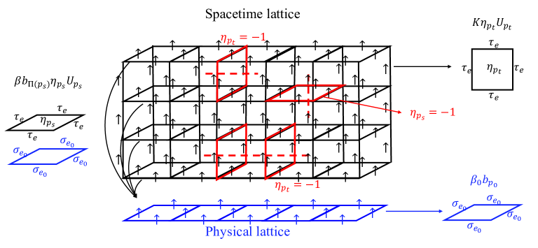
Figure 2: Illustration of the SM model we obtained in Eq. (14). The $\tau_{e}$ spins are defined on the edges of $3$-d spacetime lattice and the $\sigma_{e_{0}}$ spins lie on $2$-d physical lattice. There are three types of interactions in this model as shown in this figure. $\beta_{0}b_{p_{0}}$ is the gauge interaction term defined on the physical lattice. $K\eta_{p_{t}}U_{p_{t}}$ is the timelike gauge interaction on spacetime lattice. The $\beta b_{\Pi(p_{s})}\eta_{p_{s}}U_{p_{s}}$ term couples the spacelike gauge interaction term $U_{p_{s}}$ to the gauge interaction term $b_{\Pi(p_{s})}$ on physical lattice. The $\eta_{p}$’s set the signs of gauge interactions on spacetime lattice and they mark the position of error strings during the QEC procedure in Fig. 1(b). For example, the flipped interaction $\eta_{p}=-1$ at plaquette $p$ (red plaquette) corresponds to the presence of an error string at $p$ (dashed red line). The $\{\eta_{p}\}$ configuration follows a disorder probability (6) that comes from the randomness of Pauli errors and in syndrome measurement. The $\tau_{e}$ spins are non-locally correlated at timelike direction since all spacelike plaquette interactions $U_{p_{s}}$ along the same timelike arrow are all coupled to the same $b_{\Pi(p_{s})}$. Meanwhile, the disorder probability (6) is also correlated at time direction. Physically this is due to the fact imperfection measurement operator will change the current quantum state, which in turn affects subsequent measurement results. It is evident from the expressions (14) and (6) that the non-local correlation results from finite $\beta_{0}$, or in other words imperfect initial state preparation.

Then following the standard procedure described in Ref. Dennis et al. (2002); Bombin (2013); Chubb and Flammia (2021), we computed the probability of the topological equivalent class of error configurations and it is proportional to the partition function of an SM model

$$P([\{\eta_{p}\}])\propto\mathcal{Z}(\{\eta_{p}\})=\sum_{\{\sigma_{e_{0}}\},\{\tau_{e}\}}\exp\left[\beta_{0}\sum_{p_{0}}b_{p_{0}}\right.$$ (14)

$$\left.+\beta\sum_{p_{s}}b_{\Pi(p_{s})}\eta_{p_{s}}U_{p_{s}}+K\sum_{p_{t}}\eta_{p_{t}}U_{p_{t}}\right],\quad U_{p}=\prod_{e\in\partial p}\tau_{e}.$$

This SM model is a $3$-d $\mathbb{Z}_{2}$ gauge theory defined on the spacetime lattice coupled to a $2$-d $\mathbb{Z}_{2}$ gauge theory defined on the physical lattice, see Fig. 2. Here $\tau_{e}=\pm 1$ is a spin variable defined on each edge $e$ of the spacetime lattice. $U_{p}$ is an ordinary $\mathbb{Z}_{2}$ gauge interaction term containing four $\tau_{e}$ operators, $[\{\eta_{p}\}]$ denotes the topological equivalent class represented by $\{\eta_{p}\}$, and $\eta_{p}$ sets the sign of interaction term on each plaquette. The summation of $\{\tau_{e}\}$ configurations is the same as a summation over topologically equivalent error configurations up to a constant factor. Physically, those $\tau_{e}$ operators describe the fluctuation of error strings, since flipping $\tau_{e}$ operator is equivalent to deforming the error strings represented by $\{\eta_{p}\}$ (see detail discussions in Ref. Dennis et al. (2002); Bombin (2013)). Therefore, the model acquires a local symmetry

$$\eta_{p}\rightarrow\eta_{p}\prod_{e\in\partial p}\nu_{e},\quad\tau_{e}\rightarrow\tau_{e}\nu_{e},\quad\nu_{e}=\pm 1,$$ (15)

which ensures that topologically equivalent error configurations yield the same partition function. In order to detect the error threshold, Eq. (6) should be considered as the quenched disorder probability of interaction configuration $\{\eta_{p}\}$. Then the phase transition point of $\tau_{e}$ spins in the disordered SM model should correspond to the error threshold of the QEC model Dennis et al. (2002); Bombin (2013); Chubb and Flammia (2021). The reason for this phase transition-error threshold correspondence is as follows. Recall that the optimal decoder algorithm will select the equivalent class (of error configuration) with the largest probability or the smallest free energy. Define the free energy cost of an arbitrary non-contractible loop configuration $l=\{\eta_{p}^{l}\}$ as

$$\Delta_{l}=-\sum_{\{\eta_{p}\}}P(\{\eta_{p}\})\log\frac{\mathcal{Z}(\{\eta_{p}\cdot\eta^{l}_{p}\})}{\mathcal{Z}\{\eta_{p}\}}.$$ (16)

In the ordered phase, $\Delta_{l}$ diverges if we take the thermodynamic limit along with a disorder average. This suggests that the probability of the correct equivalent class will be far larger than that of the wrong one differed by a non-contractible loop, since the probability of an equivalent class is proportional to the partition function. Thus the optimal decoder always succeeds. In the disordered phase, however, the finiteness of free energy cost signifies the failure of the optimal decoder. A detailed explanation can be found in Ref. Chubb and Flammia (2021) for the case with stochastic errors.

V phase structure of the statistical mechanical model

Here we provide some analytical results about the SM model and its phase structure. First, we notice that the SM model has a non-local correlation at time direction originates from imperfect initial state preparation, see Fig. 2. If we set $\beta_{0}$ to $+\infty$, then the initial state is well prepared and the code space $\widetilde{\mathcal{C}}(\beta_{0})$ becomes exactly the toric code subspace. The action of following syndrome measurement operators Eq. (3) on this space yields only a global phase factor and does not change the state itself. In this case, even though the measurement outcome can still be faulty, the probability of measurement error will now become uncorrelated. This reduces to a pure probabilistic measurement error model considered in Ref. Dennis et al. (2002). At the SM model side, by taking $\beta_{0}$ to $+\infty$ we self-consistently arrive at the random plaquette gauge model (RPGM) derived also in Ref. Dennis et al. (2002).

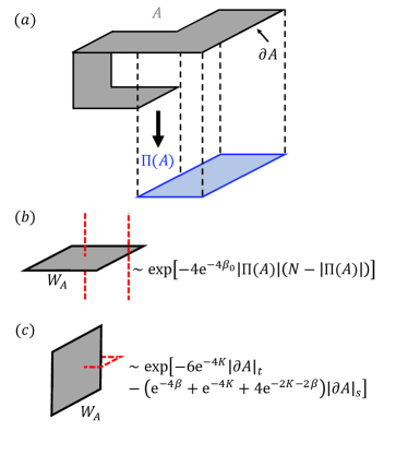
Figure 3: (a) Example of a Wilson loop. $A$ is a surface in 3D spacetime (gray) and $\partial A$ is its boundary (black), which is a closed loop. $\Pi(A)$ is the projection of surface $A$ from 3D spacetime to 2D space mod $\mathbb{Z}_{2}$. Specifically, under projection the timelike plaquettes are dropped, and an even number of spacelike plaquettes at the same space position also vanishes. The only remaining plaquettes are at the spatial locations that originally have odd numbers of spacelike plaquettes. In (b) and (c), the black lines represent Wilson loops and the red dashed lines are examples of topologically trivial error strings created by $\tau_{e}$ fluctuation. (b) A spacelike Wilson loop. In a large enough system it decays exponentially with respect to the area for any finite temperature. Note that Its scaling behavior written in the figure directly follows from Eq. (21) by constraining $A$ to a pure spacelike region. For a large region $A$, the areal decay will be much faster than the perimetric decay, so the first term in Eq. (21) dominates. This behavior is contributed by the fluctuation of infinite long timelike error strings which are able to appear at any space position (see Sec. SIV of SI Sup ). (c) A timelike Wilson loop. Its scaling behavior is obtained by constraining $A$ to a pure timelike region in Eq. (21). Under a low temperature, it decays exponentially with respect to the perimeter. Note that both timelike edges and spacelike edges are contained in the boundary of a timelike region, determining the $|\partial A|_{t}|$ term and $|\partial A|_{s}|$ term respectively. This perimetric decay behavior is mainly contributed by local error loops near the Wilson loop (see Sec. SIV of SI Sup ).

In reality, the same faulty circuits that produce the imperfect syndrome measurements also provide the imperfect initial state preparations. In this situation, i.e. with finite $\beta_{0}$, the non-local timelike correlation will lead to a different phase structure in stark contract to RPGM. In the following paragraphs, we will explore this phase structure in detail. In order to detect the phase transition of $\tau_{e}$ spins, we consider the Wilson loop

$$W_{A}=\prod_{p\in A}U_{p}=\prod_{e\in\partial A}\tau_{e},$$ (17)

which serves as the order parameter for $\mathbb{Z}_{2}$ gauge theory. Different phases of the gauge theory can be distinguished based on the fact whether the Wilson loop confines or deconfines. Here $A$ is a set of plaquettes representing a surface in spacetime. The product of $U_{p}$’s on surface $A$ equals the product of $\tau_{e}$’s on $\partial A$, which is the boundary of surface $A$ and forms a closed loop. In the conventional $\mathbb{Z}_{2}$ gauge theory Kogut (1979) the scaling behavior of Wilson loop expectation values with respect to the loop size distinguishes between the confinement (disordered) phase and the deconfinement (ordered) phase. In the deconfinement phase, it decays exponentially with respect to the perimeter of the loop,

$$W_{A}\sim\exp(-const\times|\partial A|),$$ (18)

called perimeter law. Here we use $|\cdot|$ to denote the cardinal of a set (i.e. the number of the elements of a set). For example $|\partial A|$ is the number of edges contained in $\partial A$. On the other hand, in the confinement phase, the scaling behavior of Wilson loops obeys area law,

$$W_{A}\sim\exp(-const\times|A_{min}|),$$ (19)

where $A_{min}$ is the minimal surface enclosed by $\partial A$. Here we will study the expectation value of Wilson loops in our SM model.

First, note that our SM model satisfies a generalized version of Nishimori condition Nishimori (1981, 2001), which means that the error rate parameters $(\beta_{0},\beta,K)$ in the quenched disorder probability in Eq. (6) are the same as those in the partition function in Eq. (14), respectively. Under this condition, by taking advantage of a local symmetry of the model (15), we find that (see Sec. SIII of SI Sup )

$$[\braket{W_{A}}]=[\braket{W_{A}}^{2}].$$ (20)

Here $\braket{\cdot}$ denotes the ensemble average with respect to the model Eq.(14) under a specific interaction configuration. $[\cdot]=\sum_{\{\eta_{p}\}}P(\{\eta_{p}\})(\cdot)$ represents the disorder average over interaction configurations with respect to the probability Eq.(6). The above equality suggests the absence of gauge glass phase Wang et al. (2003) ($[\braket{W_{A}}]$ obeys area law Eq.(19) but $[\braket{W_{A}}^{2}]$ obeys perimeter law Eq.(18)) so that we only need to concern about the deconfinement-confinement phase transition of $\tau_{e}$’s under Nishimori condition.

We then perform a low-temperature expansion Kogut (1979) for $[\braket{W_{A}}]$. Here low temperature means that the parameters $\beta_{0}$, $\beta$ and $K$ are sufficiently large, corresponding to small enough physical error rates. We assume $\mathrm{e}^{-\beta_{0}}$, $\mathrm{e}^{-\beta}$ and $\mathrm{e}^{-K}$ are of the same order and expand $\log[\braket{W_{A}}]$ up to the first non-vanishing order $\mathrm{e}^{-4\beta_{0}}$. We obtain the result (refer to Sec. SIV of SI Sup for more details)

$$[\braket{W_{A}}]\simeq\exp[-4\mathrm{e}^{-4\beta_{0}}|\Pi(A)|(N-|\Pi(A)|)$$ (21)

$$-\left(\mathrm{e}^{-4\beta}+\mathrm{e}^{-4K}+4\mathrm{e}^{-2\beta-2K}\right)|\partial A|_{s}-6\mathrm{e}^{-4K}|\partial A|_{t}].$$

Here $\Pi$ is defined as projection from $3$-d spacetime to $2$-d space mod $\mathbb{Z}_{2}$, illustrated in Fig. 3(a). $|\partial A|_{s}$ ($|\partial A|_{t}$) denotes the spacelike (timelike) edges $e_{s}$ ($e_{t}$) contained in $\partial A$. The low temperature expansion is done by first expanding $P(\{\eta_{p}\})$ up to $\mathrm{e}^{-4\beta_{0}}$. Then for each error configuration that appeared in the expansion, we compute the expectation value $\braket{W_{A}}$ up to the order we need. The perturbative evaluation of $\braket{W_{A}}$ is accomplished by identifying the ground state and then taking the lowest excited states into consideration. Each of these states yields a specific value of $W_{A}$. Putting all these things together, we obtain Eq. (21).

From this expression, we see that the expectation value of Wilson loops has an anisotropic scaling behavior. It deconfines at the timelike direction under low temperature but confines at the spacelike direction for any finite $\beta_{0}$ (Fig. 3). A pure timelike Wilson loop $W_{A}$ which contains only timelike plaquettes is shown in Fig. 3(c). It deconfines and decays exponentially with respect to perimeter as in a conventional $3$-d $\mathbb{Z}_{2}$ lattice gauge theory under low temperature. Meanwhile, a pure spacelike Wilson loop is shown in Fig. 3(b). For large enough system size $N$, its areal decay is faster than the perimetric decay, so the first term in Eq. (21) dominates and $[\braket{W_{A}}]$ confines as long as the temperature is finite. We notice that no matter how low the non-zero temperature is, the confinement is always maintained. Since a sufficiently high temperature should drive the system into a completely disordered phase, it will confine all Wilson loops. Specifically, we do not expect the deconfinement of spacelike Wilson loops at higher temperatures. Thus we conclude that spacelike Wilson loop confines at any finite temperature (or error rate). At a sufficiently high temperature (or error rate), we expect a phase transition that confines the timelike Wilson loop. We also noticed from Eq. (21) that this areal decay is a consequence of imperfect measurement during initial state preparation. Consistently, we find in our derivation that the area term results from the non-local timelike correlation of disorder probability Eq. (6) and partition function Eq. (14) which also depends on $\beta_{0}$ as we discussed. In comparison, if the initial state is ideally prepared ($\beta_{0}=+\infty$, corresponds to RPGM), the Wilson loops will acquire an isotropic scaling behavior, i.e. both the spacelike and timelike Wilson loops will exhibit perimetric decay at the low-temperature phase and areal decay at the high-temperature phase Dennis et al. (2002).

Here we also remark that the low-temperature expansion result shown in Eq. (21) is valid for any finite system size $N$ and region $A$, as long as the temperature (physical error rate) is sufficiently low. The subtlety is that we cannot directly take the thermodynamic limit $N\rightarrow+\infty$ in Eq. (21) because of the factor $N$ contained in the leading order. Actually, the appearance of area term $|\Pi(A)|(N-|\Pi(A)|)$ in Eq. (21) is a natural result because our space manifold is a closed surface (due to the periodic boundary condition), thus $\Pi(A)$ and its complement on $2$-d space yield the same boundary, and should be symmetric in an expression containing $|\Pi(A)|$. However under the thermodynamic limit, the phase structure of the SM model should not depend on this boundary condition, and we expect that the area law is still obeyed by spacelike Wilson loops in the low-temperature phase. A brief discussion about the analogy to the exactly solvable $2$-d $\mathbb{Z}_{2}$ lattice gauge theory can be found in Sec. SIV of SI Sup .

VI Impact on quantum error correction

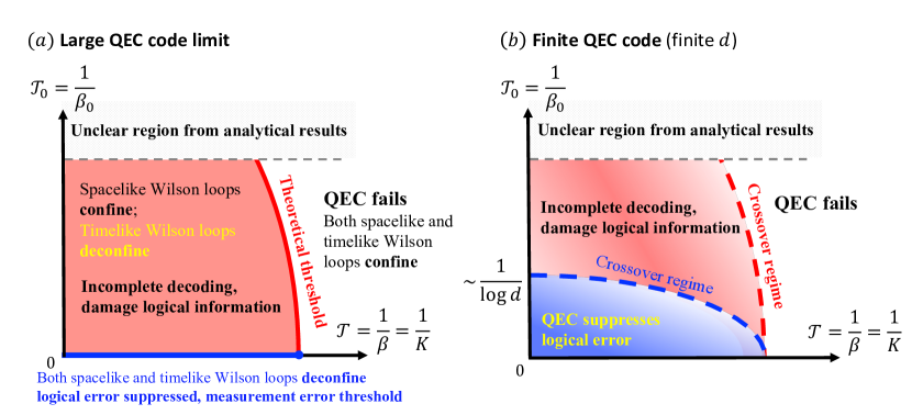
Figure 4: (a) Our estimation of the phase structure in the thermodynamic limit $T\rightarrow+\infty$ and $N\rightarrow+\infty$ while setting $\mathcal{T}=1/\beta=1/K$ and $\mathcal{T}_{0}=1/\beta_{0}$. Above the theoretical threshold (red line) QEC fails due to non-contractible logical Pauli errors. Below the theoretical threshold and above the measurement error threshold (blue line), non-contractible logical Pauli errors are suppressed. However, measurement errors are still unidentifiable through decoding a finite error history and will be confounded with Pauli errors. Note that the $\mathcal{T}$ axis where $\mathcal{T}_{0}=0$ represents the RPGM. While the theoretical threshold intersect with the $\mathcal{T}$ axis at the common RPGM phase transition point Dennis et al. (2002), we are not sure yet whether it intersect with the $\mathcal{T}_{0}$ axis. Some details at higher temperatures still requires further investigation. For completeness, we note that if $K\rightarrow+\infty$, the QEC protocol trivially succeeds as there will be no Pauli errors. On the other hand, in the scenario where $\beta\rightarrow+\infty$ but $K$ and $\beta_{0}$ are finite, the non-local measurement errors are still present and cannot be decoded when confounded with Pauli errors. (b) The phase diagram while fixing a finite code distance $d$. The phase transitions (thresholds) in Fig. 4(a) are smoothed into crossovers due to finite-size effect. Especially, the measurement error threshold becomes a finite-temperature crossover (blue dashed line), leading to a parameter region with a finite area (light blue region) that effectively suppresses logical errors. The parameters in this region should satisfy either Eq. (22) or Eq. (23) such that the non-local measurement errors will not be a problem. Specifically, the crossover condition $\mathcal{T}_{0}\sim 1/\log d$ near the $\mathcal{T}_{0}$ axis is derived from Eq. (22) (However, Eq. (22) or Eq. (23) are only approximate expressions valid in the low-temperature limit. The precise value of this crossover still requires further investigation.). Increasing $d$, this region becomes smaller and smaller and eventually sticks to the $\mathcal{T}$ axis. Above the crossover regime of measurement threshold in the light red region, the effect of non-local measurement errors on the QEC becomes non-negligible. As for the SM model side, the blue crossover detects the confinement of spacelike Wilson loops while the red crossover detects the confinement of timelike Wilson loops.

In the previous sections, we mapped our QEC model under imperfect measurement and Pauli error to an SM model and studied the phase structure of the SM model. The question is what these results imply about for QEC performance and threshold theorem. Here we provide an interpretation of these results.

First of all, knowing that there exists a confinement transition point of timelike Wilson loops in the limit $T\rightarrow+\infty$ and $N\rightarrow+\infty$, we want to ask how it relates to the logical error rate and error threshold. In fact, we find that the logical error rate is suppressed at the low-temperature phase. Note that the fluctuation of topologically trivial error strings is described by the fluctuation of $\tau_{e}$’s (refer to the discussion of Eq. (15)). Each fluctuated spin configuration will contribute to the expectation value of Wilson loop. So the behaviors of Wilson loops reflect features of error string fluctuations. In our derivation of low-temperature expansion (also see Sec. SIV of SI Sup ), we find that: 1) the areally decaying behavior of spacelike Wilson loop results from non-local timelike error strings like in Fig. 3(b); 2) the non-local timelike strings and other local error loops appear in a relatively independent manner at sufficiently low temperatures. Therefore, those local error loops are compressed and are unlikely to stretch to arbitrarily large. Specifically, the fluctuating error strings cannot extend arbitrarily long in space direction. Since the non-contractible loops can only wind around spacelike directions, we still expect their free energy cost, i.e. $\Delta_{l}$ shown in Eq. (16), to diverge, hence the logical error rate approaches zero. Increasing the temperature, there should be a transition point where spacelike error strings become extending along the whole system and $\Delta_{l}$ becomes finite, and thus the probability of logical error acquires a finite value. This transition point of $\Delta_{l}$ should be exactly the confinement point of timelike Wilson loops. Since the confinement transition point of timelike Wilson loops separates different behavior of logical error rate in the limit $T\rightarrow+\infty$ and $N\rightarrow+\infty$, it is appealing to identify this transition point as the threshold, which we refer to as theoretical threshold. However, this threshold, which we will find later, does not capture the correctability of measurement error.

Table 1: Comparison between our case and the case with the stochastic measurement error model Dennis et al. (2002). Note that although the measurement noises of the two models are different at the physical level, their error correction properties and corresponding SM models will become equivalent when we set the initial state in our model to be ideal ($\beta_{0}\rightarrow+\infty$).

We want to emphasize that, only for the infinite-time syndrome scenario, the theoretical threshold in our model can faithfully determines the success of QEC as we discussed in the last paragraph. However, due to the unidentifiable even below the theoretical threshold, the decoding procedure fails while considering a finite time syndrome information. In the infinite-time case, the decoder takes an infinite error history to enhance the power of QEC. But in reality, we can only store finite error history, where the areal decay of spacelike Wilson loops drastically affects the QEC. Roughly speaking, in the real world the decoder must be applied to a finite time interval of size $T$. Then problems arise while trying to correct measurement errors in the finite-time scenario. Recall that the areal decay of spacelike Wilson loops signifies error strings can stretch infinitely along the timelike direction. This suggests that measurement errors can easily extend from the beginning to the end and become generally undistinguishable from Pauli errors. For example, the true syndrome of a single Pauli error string will be two non-local timelike strings starting from its boundary points. Meanwhile, this syndrome can also be created by non-local measurement errors, which could occur with a probability close to the one of the Pauli string and cannot be suppressed by large $T$. The consequence is that the decoder might mix up these two situations with a finite probability and leave this Pauli error uncorrected (the correction operator determined by the decoder will not be containing this Pauli string). From this example, we infer that due to the presence of non-local measurement errors, there will be Pauli errors remaining uncorrected at the end of the QEC procedure, which means that the combined strings of the Pauli error operator and correction operator will still have an amount of open ends. If these open-ended strings anticommute with logical $Z$ operators, it will damage the logical information $\ket{L}$ (refer to the discussion of Eq. (5)). This situation does not have much difference from the case when only a single round of syndrome measurement is performed ($T=1$), since the probabilities of non-local measurement errors do not depend on $T$.

We conclude that for a large system size $N$, the ability to identify measurement errors cannot be enhanced by increasing the number of syndrome measurement rounds, even below the theoretical threshold. This is in stark contrast to the case with only stochastic errors Dennis et al. (2002), where the perimeter law for both the spacelike and timelike Wilson loops guarantees the achievement of an effective error correction with a finite error history whenever the error rate is below the theoretical threshold. In our case, the inability to correct measurement errors is caused by the finite value of $\beta_{0}$, i.e. the imperfection of initial state preparation; so we refer to $\beta_{0}=+\infty$ as the measurement error threshold of our error model. Setting $\beta_{0}=1/\mathcal{T}_{0}$ and $\beta=K=1/\mathcal{T}$, a sketch of the phase diagram is shown in Fig. 4(a). In addition, an overall comparison of our error model and the model in Ref. Dennis et al. (2002) can be found in Tab. 1.

As we have mentioned in the above paragraphs, the measurement errors are unidentifiable even at low temperatures, in the sense that the multi-round syndrome measurement protocol will not be better than a single-round one, i.e. $T=1$ or a 2D decoder. So one might ask how the QEC behaves when $T=1$. Suppose the QEC initial state is the imperfect logical $00$ state $\ket{\widetilde{\Psi}}=\ket{\widetilde{00}}=(\ket{\widetilde{++}}+\ket{\widetilde{+-}}+\ket{\widetilde{-+}}+\ket{\widetilde{--}})/2$, we estimate the impact of measurement errors on the logical fidelity, that is the fidelity between the final state and the initial state. Consider the scenario where the temperature is low and the system is of considerable size. In accordance with the preceding discourse, A Pauli error on a single physical qubit will be confounded with measurement errors having the same syndrome by the decoder. Consequently, the Pauli error will remain uncorrected. If the uncorrected Pauli error intersects with a logical Pauli $Z$ operator, it acts as a logical error on the logical information $\ket{L}$ (refer to Eq. (5)), leading to a logical fidelity $\sim 0$. But if the Pauli error locates elsewhere on the lattice, one may check that the effects of the Pauli error and the measurement operator with the same syndrome complement each other and lead to a fidelity $\sim 1$, since they both flip the same stabilizer bits in Eq. (5) but do not affect the logical information $\ket{L}$. Average all error configurations, since the number of configurations that a Pauli error intersects with logical $Z$ is proportional to $d=\sqrt{N}$, we anticipate that the logical fidelity behaves as $1-const\times d$. The logical fidelity is suppressed by a large distance, which is a signal that the QEC system is above the ture threshold (measurement error threshold in our work). Here the constant depends on the physical error rates $\beta_{0}$, $\beta$ and $K$ but does not depend on the distance $d$, and it should drop to $0$ when the initial state is ideal, $\beta_{0}\rightarrow+\infty$.

In contrast, we compare it with the $T=1$ case of Ref. Dennis et al. (2002), the 2D decoder suffering from stochastic measurement errors. The decoder in this case also mixes up a Pauli error with probabilistic measurement errors, but their effects do not complement each other, since the probabilistic measurement error is just noise on the classical readouts and does not affect the quantum state. Consequently the logical fidelity scales as $1-const\times d^{2}$, where the constant depends on the probability of Pauli and measurement errors. This logical fidelity is also above the threshold. Surprisingly, it is worse than the one of our model. However, the logical fidelity under stochastic errors can be improved by increasing $T$ and arrives at an effective QEC when $T\gg d$ Dennis et al. (2002), which is not possible in our model.

One might argue that although the non-local measurement errors suppress logical fidelity, the correction of other local errors might lead to other terms that increase with $d$ and compete with non-local measurement errors. However, the non-local measurement error suppression should be the leading order contribution in the low-temperature limit. Moreover, if the system lies above the blue crossover in the light red region in Fig. 4(b), the effect of non-local measurement errors overweights other local errors. Thus we believe that the non-local measurement error suppression could overweight other terms in that region. Nonetheless, these statements are not rigorous proofs and require further studies.

For a small code with limited system size $N$, we infer from Eq. (21) that the above problem might be circumvented with the limit

$$d\ll\mathrm{e}^{\beta_{0}},$$ (22)

or

$$d\ll[\mathrm{e}^{4\beta_{0}}(\mathrm{e}^{-4\beta}+\mathrm{e}^{-4K}+4\mathrm{e}^{-2\beta-2K})]^{1/3}.$$ (23)

Here $d$ is the code distance and $N=d^{2}$. The first bound is derived by assuming the areal term in Eq. (21) is negligible

$$e^{-4\beta_{0}}|\Pi(A)|(d^{2}-|\Pi(A)|)\ll 1,$$ (24)

for all spacelike Wilson loops $A$. The l.h.s. maximizes when $A$ is half the size of the spatial lattice $|\Pi(A)|=d^{2}/2$. Substitute $|\Pi(A)|=d^{2}/2$ into the above expression, we obtain Eq. (22) ignoring a constant factor. Physically, Eq. (22) is interpreted as the impact of measurement error itself on the system is ignorable. The second bound is derived by considering when the perimetric decay will be faster than the areal decay in Eq. (21) for a spacelike Wilson loop,

$$e^{-4\beta_{0}}|\Pi(A)|(d^{2}-|\Pi(A)|)$$ (25)

$$\ll\left(\mathrm{e}^{-4\beta}+\mathrm{e}^{-4K}+4\mathrm{e}^{-2\beta-2K}\right)|\partial A|_{s}.$$

Still we require $A$ to be half of the spatial lattice, $|\Pi(A)|\sim d^{2}$ and $|\partial A|_{s}\sim d$. Thus we obtain Eq. (23). Physically, Eq. (23) is interpreted as the influence of non-local error strings is not significant compared to other local error strings. If either of these two bounds is satisfied, we anticipate that the ability of our QEC procedure to detect measurement errors will be similar to that of Ref. Dennis et al. (2002). To satisfy either Eq. (22) or Eq. (23), the imperfection of initial state preparation must be negligible or much smaller than the syndrome measurement imperfection and Pauli error rate. Even then the code distance is still upper bounded if we fix the error parameters $\beta_{0}$, $\beta$ and $K$. Usually, when performing QEC, we anticipate increasing code distance to suppress the logical error rate Fowler et al. (2012). However, for the important error problem considered here, Eq. (22) and Eq. (23) form bounds that prevent the code from scaling up. Equivalently if we fix $d$ and vary the error parameters, we obtain the phase diagram in Fig. 4(b). It is noteworthy that the region enabling pragmatic error correction only experiences a gradual reduction as increasing the code distance, i.e. $\sim 1/\log d$, which is not excessively frustrating.

VII discussion

In this work, we discuss the imperfect measurement problem based on the circuit shown in Fig. 1(d) (e.g. for $B_{p_{0}}$), which allows us to conduct an analytic study. In fact, the circuit shown in Fig. 1(c), which contains only two-qubit gates rather than a five-qubit evolution in our simple model, is more realistic. Ref. Yang and Liu (2022) discussed an imperfect measurement model which mimics the behavior of superconducting quantum computation systems. The $CNOT$ gate is divided into a $CZ$ gate and two Hadamard gates, $CNOT=H(CZ)H$ where $H$ is the Hadamard gate acting on the target qubit (ancilla qubit in our setup). Each $CZ$ gate is implemented by a time evolution

$$U=\exp\left[-\mathrm{i}\frac{t}{4}\left(s^{z}\otimes\sigma_{i}^{z}-s^{z}\otimes I-I\otimes\sigma^{z}_{i}+I\otimes I\right)\right]$$ (26)

Here $s$ labels the ancilla qubit and $\sigma_{i}$, $i=1,2,3,4$ labels the four data qubits. It recovers the $CZ$ gate when $t=\pi$. Assume the final ancilla measurement has an outcome $s=\pm 1$, the corresponding action on data qubits is

$$M_{s}=\bra{s}H\exp\left[-\mathrm{i}\frac{t}{4}\sum_{i}\left(s^{z}\otimes\sigma_{i}^{z}-s^{z}-\sigma^{z}_{i}+I\right)\right]H\ket{0}=\frac{1}{2}\left(1+s\mathrm{e}^{-\mathrm{i}2t}\cos^{4}\frac{t}{2}+s\mathrm{e}^{-\mathrm{i}2t}\sin^{4}\frac{t}{2}B_{p_{0}}\right)$$ (27)

$$\times\left(1-\frac{\mathrm{i}s\mathrm{e}^{\mathrm{i}2t}\sin\frac{t}{2}\cos^{3}\frac{t}{2}+\mathrm{i}\sin\frac{t}{2}\cos^{7}\frac{t}{2}+\mathrm{i}\sin^{7}\frac{t}{2}\cos\frac{t}{2}}{\left(s\mathrm{e}^{\mathrm{i}2t}+\cos^{4}\frac{t}{2}\right)^{2}-\sin^{8}\frac{t}{2}}\sum_{i}\sigma^{z}_{i}-\frac{\sin^{2}\frac{t}{2}\cos^{2}\frac{t}{2}}{s\mathrm{e}^{\mathrm{i}2t}+\cos^{4}\frac{t}{2}+\sin^{4}\frac{t}{2}}\sum_{i<j}\sigma^{z}_{i}\sigma^{z}_{j}\right.$$

$$+\left.\frac{\mathrm{i}s\mathrm{e}^{\mathrm{i}2t}\sin^{3}\frac{t}{2}\cos\frac{t}{2}+\mathrm{i}\sin^{3}\frac{t}{2}\cos^{5}\frac{t}{2}+\mathrm{i}\sin^{5}\frac{t}{2}\cos^{3}\frac{t}{2}}{\left(s\mathrm{e}^{\mathrm{i}2t}+\cos^{4}\frac{t}{2}\right)^{2}-\sin^{8}\frac{t}{2}}\sum_{i<j<k}\sigma^{z}_{i}\sigma^{z}_{j}\sigma^{z}_{k}\right).$$

When $t=\pi$, one may check that the above expression reduces to the correct projection $(I+sB_{p_{0}})/2$. When $t\neq\pi$, $M_{s}$ stands for an imperfect measurement operator. We notice that in its expression the first factor $1+s\mathrm{e}^{-\mathrm{i}2t}\cos^{4}(t/2)+s\mathrm{e}^{-\mathrm{i}2t}\sin^{4}(t/2)B_{p_{0}}$ is similar to the imperfect measurement operator discussed in Eq. (3) $\exp({\beta s_{p_{0}}B_{p_{0}}/2})=\cosh(\beta/2)+s_{p_{0}}\sinh(\beta/2)B_{p_{0}}$. However, there is an additional factor, which can be viewed as coherent errors appearing on data qubits. So while discussing error correction, aside from the consequence talked about before, coherent errors will do more damage to the error correction procedure and lead to worse performance. We also notice that under this realistic measurement model, if we define logical states by applying logical operators to the imperfect initial state, those states will not be orthogonal to each other, which makes it much hard to analyze theoretically.

In all, by mapping the standard QEC procedure under imperfect measurement to an SM model, we find two finite temperature phases that have different QEC performances. The high temperature (high physical error rate) phase signifies the failure of QEC caused by non-contractible error strings. In the low temperature (low physical error rate) phase, the measurement errors cannot be identified through decoding syndrome outcomes of finite rounds due to imperfect initial state preparation, which could result in the failure of QEC in the large code distance limit. For finite $d$ there will be a parameter region $\sim\log d$ that logical errors remain suppressed. In addition, we remark that studying a different measure of logical error rate, such as average gate fidelity Emerson et al. (2005) or diamond norm Aharonov and Ben-Or (1999), might provide a better knowledge of how the results in this article affect error threshold in the current problem, which is very different since imperfect measurement of stabilizers not only causes faulty syndrome outcomes but also changes the quantum state as we discussed. Therefore, further work concerning these issues still needs to be developed. In addition, we notice that as shown in Ref. Zhu et al. (2022); Lee et al. (2022), the imperfect initial state preparation leads to the absence of long-range entanglement. Meanwhile, the imperfect initial state is also the source of the ill performance in our QEC model. These phenomena are both related to the confinement of certain Wilson loop observables. Therefore, another intriguing question is that what role the long-range entanglement could play in the threshold theorem of the general topological QEC codes?

See pages 1 of SuppInfo-LGT.pdf See pages 2 of SuppInfo-LGT.pdf See pages 3 of SuppInfo-LGT.pdf See pages 4 of SuppInfo-LGT.pdf See pages 5 of SuppInfo-LGT.pdf See pages 6 of SuppInfo-LGT.pdf See pages 7 of SuppInfo-LGT.pdf See pages 8 of SuppInfo-LGT.pdf See pages 9 of SuppInfo-LGT.pdf See pages 10 of SuppInfo-LGT.pdf See pages 11 of SuppInfo-LGT.pdf See pages 12 of SuppInfo-LGT.pdf See pages 13 of SuppInfo-LGT.pdf See pages 14 of SuppInfo-LGT.pdf See pages 15 of SuppInfo-LGT.pdf See pages 16 of SuppInfo-LGT.pdf See pages 17 of SuppInfo-LGT.pdf