Planning Multiple Epidemic Interventions with Reinforcement Learning

Abstract

Combating an epidemic entails finding a plan that describes when and how to apply different interventions, such as mask-wearing mandates, vaccinations, school or workplace closures. An optimal plan will curb an epidemic with minimal loss of life, disease burden, and economic cost. Finding an optimal plan is an intractable computational problem in realistic settings. Policy-makers, however, would greatly benefit from tools that can efficiently search for plans that minimize disease and economic costs especially when considering multiple possible interventions over a continuous and complex action space given a continuous and equally complex state space. We formulate this problem as a Markov decision process. Our formulation is unique in its ability to represent multiple continuous interventions over any disease model defined by ordinary differential equations. We illustrate how to effectively apply state-of-the-art actor-critic reinforcement learning algorithms (PPO and SAC) to search for plans that minimize overall costs. We empirically evaluate the learning performance of these algorithms and compare their performance to hand-crafted baselines that mimic plans constructed by policy-makers. Our method outperforms baselines. Our work confirms the viability of a computational approach to support policy-makers.

1 Introduction

Public health policymakers face a myriad of challenges when designing and implementing intervention plans to curb the spread of an epidemic. First, each disease is unique: what works to contain an Ebola outbreak — a disease spread through direct contact with infected bodily fluids — is different from what works to contain a flu outbreak. Second, the efficacy and effectiveness of interventions may vary widely even for similar diseases: the flu vaccine’s effectiveness can vary from 40% to 60% depending on how well the vaccines are matched to the current season’s flu strains Oxford Vaccine Group (2020). Third, the disease or our understanding of its dynamics may evolve as new disease variants arise. The new variants may entail changes in intervention plans to reflect the changes in the disease’s transmissibility or severity Karim et al. (2021). Finally, quantifying the cost and benefit of a combination of interventions is difficult even after an extensive post-hoc analysis Lee et al. (2019) In short, there are no template intervention plans that can be universally and directly applied across all disease outbreaks, regions and populations.

Nevertheless, in practice, research supporting policy makers often consists of the simulation of a small set of predefined and relatively coarse intervention plans on a carefully-calibrated epidemiological model to assess and compare the economic cost and disease burden of each plan Ferguson et al. (2020). While this approach has the virtue of simplicity, it disregards the large space of potential policies.

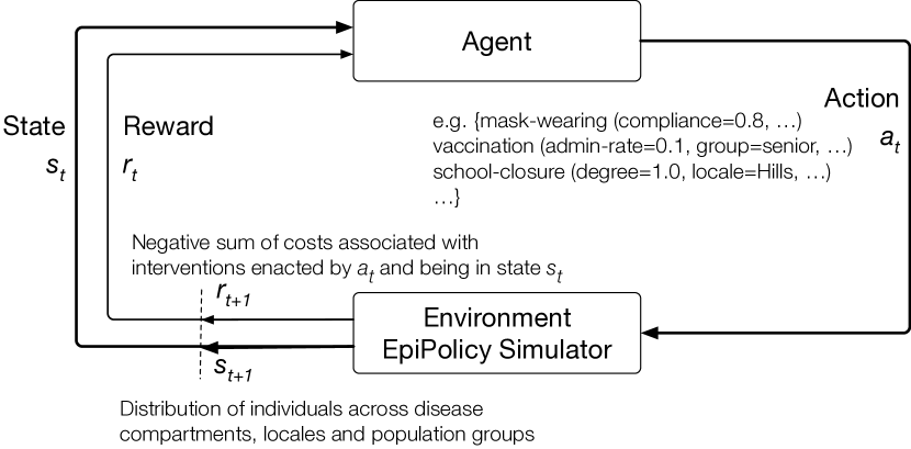
Figure 1: The agent-environment interaction in the Markov decision process formalizing the epidemic planning problem.

In contrast to the approach of choosing a plan from a set of predefined ones, we consider the following algorithmic challenge: can we automatically and efficiently search for an optimal schedule of interventions that minimizes overall disease burden and economic cost? An exact solution to this combinatorial search problem is intractable. With a one-year planning horizon of week-long timesteps, and only three binary interventions (e.g. close or open schools; close or open borders; enforce or relax mask-wearing mandates), there are $8^{52}$ plans to consider! Furthermore, many interventions have inherently continuous parameters (e.g. the number of vaccines to administer daily ranges from 0 to the available number of doses, or the distance between individuals in a physical distancing intervention may range from 0 to 10 meters) and policy-makers may disagree on how to discretize them.

Theoretical approaches that rely on dynamic programming techniques Littman et al. (2013) or Pontryagin’s maximum principle Perkins and España (2020); Obsu and Balcha (2020) neither scale nor generalize to complex disease models (i.e. a large continuous state space) with a diverse set of candidate interventions. Recent works have examined the application of reinforcement learning (RL) to intervention planning. We can classify these works into ones that built disease simulators that enable control by an RL agent Kompella et al. (2020); Libin et al. (2020), or

programmable optimization toolboxes Colas et al. (2020). None of these works allows a large continuous disease state space, a multi-intervention continuous action space, and the ability to simulate different diseases and interventions as shown in Table 5.

By contrast, we rely on an existing framework, EpiPolicy Tariq et al. (2021), that can simulate (i) disease-spreading interactions across regions for a given disease model and population and (ii) programmatically-defined interventions with free parameters that determine their effects and costs. This allows us to empirically examine the rich problem of controlling multiple interventions with RL that none of the prior works have examined.

Contributions & Paper Outline.

We present two main contributions:

(i)   A demonstration of how to use reinforcement learning to construct epidemic intervention plans over complex continuousdisease and population models, with multiple interventions. To achieve this, we formulate the problem as a Markov Decision Process (MDP) in Section 2. We explore the space of possible RL approches in Section 2.2, to select two algorithms (PPO, SAC) that fit our problem and we empirically tune them (Section 3). We present promising empirical results on a wide range of epidemic planning problems of varying complexity both in terms of the state space and action space (Section 3.2).

(ii)   A benchmark for reinforcement learning and epidemiology researchers (Section 3.1). The environments in our benchmark represent real disease models and interventions. Moreover, the benchmark can be easily extended to include other disease models or interventions. The code, data, and experiments can be found in our GitHub repository. The benchmark was motivated by and built in consultation with public health officials, so it should be useful to computational epidemiology researchers. In addition, the benchmark provides a testing point for RL algorithms allowing further research into improving their performance.

2 Problem Formulation

We frame the epidemic plan optimization problem as a Markov Decision Process (MDP), where an agent learns an (approximately) optimal policy or plan by interacting with a simulator of the natural disease environment. Figure 1 illustrates the agent-environment interaction in our application. The MDP formalizes the sequential decision-making process of epidemic planning, where an action — a full parameterization of the set of interventions — at each time step (e.g., a week) influences the immediate costs (e.g., the costs associated with vaccinating a certain number of individuals) and rewards (e.g.,the avoidance of the cost of sick days due to increases in the infectious populations). Thus, each action influences both the subsequent state and future costs and rewards.

2.1 The Markov Decision Process

An MDP is a 4-tuple $\langle\mathcal{S},\mathcal{A},p(s_{t+1}|s_{t},a_{t}),r(s_{t},a_{t},s_{t+1})\rangle$:

$\blacktriangleright$ State: $\mathcal{S}$ is the state space. In our application, a state $s_{t}$ is the distribution of the population across different disease compartments (e.g., infected, recovered, hospitalized, etc.) including their regional (e.g, a particular state or province) and group subdivisions (e.g., adult, senior, child, male, female, etc.).

$\blacktriangleright$ Action: $\mathcal{A}$ is the action space. An action $a_{t}$ is the set of applied interventions at time $t$ and their parameter values (e.g. 82% school closure).

$\blacktriangleright$ State-transition: $p(s_{t+1}|s_{t},a_{t})$ is a function $p:\mathcal{S}\times\mathcal{S}\times\mathcal{A}\rightarrow[0,1]$. The probabilities given by $p$ characterize the dynamics of the environment. In our setting, this function is evaluated by executing a deterministic simulator with the state $s_{t}$ and action $a_{t}$ as inputs for a single time step. fixed current state and action $s_{t},a_{t}$. Since the future state $s_{t+1}$ depends only on the current state $s_{t}$ and the applied action $a_{t}$, the Markov property is satisfied.

$\blacktriangleright$ Reward: $r(s_{t},a_{t},s_{t+1})$ is a function $r:\mathcal{S}\times\mathcal{A}\times\mathcal{S}\rightarrow\mathbb{R}$. The reward of applying action $a_{t}$ to state $s_{t}$ to reach state $s_{t+1}$ is simply the negative of the sum of the costs associated with implementing the interventions in the action $a_{t}$ and the costs associated with being in a certain state $s_{t}$ to state $s_{t+1}$ for the time step.

2.1.1 The Simulator

An epidemic simulator for compartmental disease models approximates the progression of the disease in the face of the interventions. Concretely, it defines the behavior of the state-transition function, $p$, of the MDP.

For our application, we require a simulator that:

(i)   uses a deterministic compartmental disease model. Typical compartments will be susceptible (S), infected (I), and recovered (R), with known transition rates such as recovery rate and infection rate. The compartmental model describes how disease spreads in a population with predefined demographic and geographic characteristics using ordinary differential equations (ODEs).

(ii)  simulates the results of programmatically-defined and parameterized interventions (the actions) in terms of their effects on the transition rates and on the distribution of the population across the compartments. The behavior (effects and costs) of an intervention should be modifiable by its control parameters.

(iii)  exposes the simulator’s internal state in terms of the distribution of the population across the different compartments, its incurred costs as a function of the cost of each state (e.g., the estimated dollar cost of $x$ individuals being sick), and the cost of interventions applied (e.g., each vaccine administered costs $y$ dollars).

The first requirement follows from scalability considerations. Stochastic population models better capture randomness but their differential equations are more expensive to solve. In addition, they are not as scalable as deterministic models for RL training where many experiences need to be simulated. Agent-based models are also difficult to scale and are often limited to population sizes of at most one million.

Figure 2 illustrates a compartmental disease model with four compartments: susceptible (S), infectious (I), recovered (R) and two vaccinated compartments (V1, V2) one for each dose in a disease with a two-dose vaccination regiment. Transition rates are the ODE parameters that control the progression of the population from one compartment to another. For example, three parameters in Figure 2: $\beta$ the transmission rate, $\nu$ the loss of immunity rate, and $v_{1}$ the first-dose vaccination rate, together control the rate of change in the susceptible (S) compartment through the following ODE: $\frac{dS}{dt}=\frac{-\beta IS}{N}+\nu R-v_{1}S$. Here $N$ is the total population count and $S,I,R$ are the number of individuals in their respective compartments at a given time.

We assume that the transition rates are known and provided a priori. Inferring their values, sometimes called model calibration, is its own sub-field within epidemiology Hazelbag et al. (2020).

The second requirement enables the RL agent to explore and control how each intervention is applied by setting its control parameters.

Finally, the third requirement (exposure to a simulator’s internal state) enables the RL agent to evaluate the rewards of an intervention plan.

We use EpiPolicy as our epidemic simulator because it satisfies the above requirements Tariq et al. (2021); Mai et al. (2022).

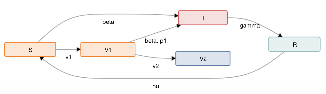
Figure 2: The compartmental SIRV model with five compartments: susceptible (S), infectious (I), recovered (R) and two vaccinated compartments (V1, V2) for a disease with a two-dose vaccination regiment. Note the model has a transition edge from R to S annotated with the immunity loss transition rate $\nu$ indicating the possibility of reinfection in this model.

We note that in our formulation both the action space and the state space are continuous and bounded. For example, interventions like school closures are controlled by a degree of the school closure parameter that ranges from 0 to 1. Given a fixed population size $N$, the number of individuals across the compartments and their regional or demographic subdivisions (e.g. male/female or child/adult/senior) range from $0$ to $N$

$\blacktriangleright$ Plan or Schedule. An epidemic intervention plan is simply the sequence of actions $a_{0},...a_{T}$ applied over a fixed time horizon $T$. Given an initial state $s_{0}$, the MDP, and the plan enacted by the agent, we can construct a trajectory: $s_{0},a_{0},r_{0},s_{1},a_{1},r_{1},...s_{T},a_{T},r_{T}$. The cumulative reward of the plan is simply the (discounted) sum of all the rewards from $r_{0}$ to $r_{T}$: $r_{0}+r_{1}\gamma+r_{2}\gamma^{2}+...+r_{T}\gamma^{T}$ where $\gamma\in[0,1]$ is the discount factor. In epidemic modelling, an action can have significant long-term consequences (like uncontrolled disease spread). For that reason, we set the discount factor at 0.99 to reflect the importance of mitigating the costs of an epidemic not only in the short term but also toward the end of the time horizon.

2.2 The Agent & Solution Strategies

The goal of the agent is to find an optimal epidemic intervention plan that minimizes overall cost. While formulating epidemic planning as an MDP problem is straightforward, solving the MDP problem is not. We found that only Actor-Critic methods efficiently solve MDPs for planning epidemic interventions: analytical approaches do not extend beyond simple epidemiological models and tree search approaches suffer from inefficient sampling which require significant computational resources.

Analytical Approaches.

An MDP with a continuous action space and a continuous state space can sometimes be solved via the partial derivatives of the Bellman Optimality Equation with respect to the action space Rao (2020). This requires that the reward function be expressable as a closed-form function of the current state $s_{t}$ and action $a_{t}$, which in turn requires an analytical solution of the ODE system. An analytical solution may be possible when the ODE system is simple enough such as in the three-compartment SIR model of Barlow and Weinstein (2020), but it is not possible in general. Dynamic programming approaches as well as Pontryagin’s maximum principle have also been used in the optimal control of simple epidemiological models in Perkins and España (2020); Obsu and Balcha (2020).

Tree Search.

Natively, Monte Carlo Tree Search (MCTS) Kocsis and Szepesvári (2006) requires both the state space and the action space to be discrete.

Discretization of the action space requires domain knowledge, however. In our work with public health officials, we often found disagreement regarding the granularity and the values of such discretizations.

Moreover, MCTS suffers from low sampling efficiency. At each time step, MCTS estimates the value of a certain action through many Monte Carlo random plan simulations. The more simulations, the more accurate the estimate. This tradeoff implies that as the action space grows (with more interventions or with finer-grained discretizations), the computational resources have to increase exponentially in order to obtain reasonable coverage. Without good coverage, plans generated by MCTS will be much more costly than simple hand-crafted plans.

Actor-Critic Methods.

In contrast to the planning approaches discussed above, we consider an agent that produces a policy.

$\blacktriangleright$ Policy: $\pi:\mathcal{S}\times\mathcal{A}\rightarrow[0,1]$ is a probability distribution on the actions given a state $s$.

In actor-critic methods, the agent is both a critic that learns the value of a specific state or an action, often with a neural network, and an actor, that learns a policy, also through a neural network, as guided by the critic. The agent generates an intervention plan or schedule for an initial state $s_{0}$, by sequentially sampling actions $a_{t}\sim\pi(s_{t})$, simulating the next state $s_{t+1}\sim p(s_{t},a_{t})$, and computing the reward $r_{t}=r(s_{t},a_{t},s_{t+1})$, repeatedly until the time horizon $T$.

Actor-Critic methods theoretically converge to the local maximum of the reward function Konda and Tsitsiklis (1999). They inherently support continuous state and action spaces as the neural networks representing the actor and the critic support continuous input and output values. State-of-the-art actor-critic methods such as Soft Actor-Critic (SAC) Haarnoja et al. (2018) or Proximal Policy Optimization (PPO) Schulman et al. (2017) have been shown to have good learning performance in a wide range of reinforcement learning tasks Wang et al. (2019). These methods, however, are sensitive to the setting of their hyperparameters, requiring extensive experimentation and benchmarking to appropriately tune them. In the following section, we test these methods on a new benchmark consisting of six different epidemic environments.

Intervention		Control Parameter				Action Spaces
				Range	Description of control parameter’s effect	A	B
1	Mask-wearing	Compliance Degree	$m$	[0, 1]	Affects the transition from S to I by modifying the transmissibility $\beta$ rate. Higher compliance reduces the transmissibility rate as follows: $(1-Rm)\beta$, where $R\approx 0.8$ is the reduction in transmission rate at full compliance ($m=1$).	Y	Y
2	Vaccination	Administration Rate	$v$	[0, 1]	Moves $vC$ individuals from S to R in SIR, S to V1 in SIRV and S to V in C15. $C\approx 10,000$ is the maximum number of doses available.	Y	Y
3	School closure	Remote learning proportion	$s$	[0, 1]	Higher proportions lower infectious interactions within school facilities; $s=0$ means no remote learning/school closure.		Y
4	Workplace closure	Remote working proportion	$w$	[0, 1]	Higher proportions lower infectious interactions within workplace facilities; $w=0$ means no workplace closures.		Y

Table 1: The four interventions in the different action spaces $A,B$. The costs associated with each intervention can be found in table 3.

	Baseline Policies
	Aggressive	Lax	Random
$m$	0.8	1	$\sim U(0,1)$
$v$	85% population in 9 months	70% population in 12 months	$\sim U(0,1)$
$s$	if $t\in[0,120]$ then 1, 0.5 otherwise;	0	$\sim U(0,1)$
$w$	if $t\in[0,120]$ then 1, 0.5 otherwise;	0	$\sim U(0,1)$

Table 2: The Aggressive and the Lax baseline policies have set control parameter settings for the interventions, while the values for the Random baseline are sampled uniformly at random from the parameter’s range.

Intervention	Cost
Mask-wearing	0.05$ per person wearing mask per day
Vaccination	40$ per person getting vaccinated
School closure	1.8$ per affected person per day
Workplace closure	1.8$ per affected person per day
Disease State	Cost
Infections	173$ per infectious person per day
Hospitalizations	250$ per hospitalized person per day
Fatalities	100,000$ for each fatality

Table 3: The four interventions under consideration with their respective cost as well as the disease burden cost.

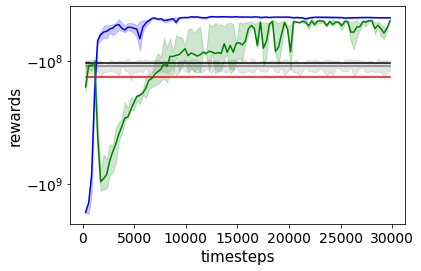
(a) SIR-A

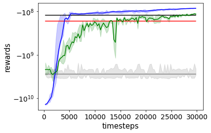
(b) SIRV-A

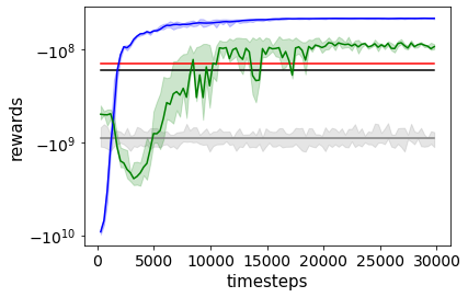
(c) C15-A

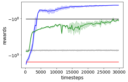
(d) SIR-B

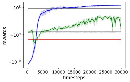
(e) SIRV-B

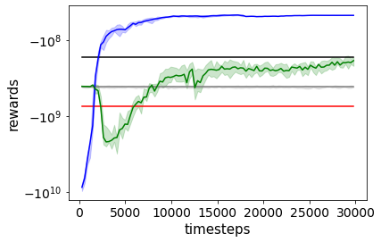
(f) C15-B

Figure 3: The cumulative reward (minimizing cost) of PPO and SAC over 30,000 training timesteps, averaged over four random seeds, We also plot the cumulative rewards of the three baseline policies, Lax, Aggressive and Random. In all scenarios, PPO outperforms both SAC and the baseline policies.

Policy		SIR-A	SIR-B	SIRV-A	SIRV-B	C15-A	C15-B
Random	$\max$	$-94.1$	$-693.5$	$-1008.3$	$-717.4$	$-559.3$	$-387.7$
	$\mu\pm\sigma$	$-110.4\pm 20$	$-745.5\pm 46.6$	$-2798.3\pm 1049$	$-811.9\pm 61.8$	$-905.2\pm 291$	$-415.4\pm 20.5$
Aggressive		$-135.9$	$-1576$	$-166.3$	$-1577.1$	$-139.9$	$-742.9$
Lax		$-104.4$	$-104.2$	$-122.4$	$-115.6$	$-167.6$	$-166.6$
SAC	$\max$	$-43.4$	$-73.4$	$-99.9$	$-169.2$	$-65.6$	$-128.6$
	$\mu\pm\sigma$	$-45.3\pm 1.9$	$-92.2\pm 12.6$	$-108.6\pm 5.7$	$-200.4\pm 22.7$	$-73.7\pm 7.2$	$-176.7\pm 53.7$
PPO	$\max$	$-42.9$	$-42.1$	$-82.2$	$-78.9$	$-45.3$	$-45.2$
	$\mu\pm\sigma$	$-43.3\pm 0.2$	$-42.5\pm 0.3$	$-83.4\pm 1.2$	$-81.2\pm 1.5$	$-45.7\pm 0.47$	$-46.2\pm 0.52$

Table 4: Maximum, mean and standard deviation of the highest cumulative rewards (expressed as negative costs) achieved by each reinforcement learning algorithm or baseline policy across four different random seeds. All maximum and mean rewards and standard deviations are in millions of dollars ($10^{6}$).

3 Empirical Evaluation

3.1 The Benchmark

The benchmark described here is largely inspired by a collaboration with a public health entity through a non-disclosure agreement that preserves their anonymity. Our public health colleagues wanted guidance on multiple interventions for mitigating different diseases. These interventions had control parameters that described the degree of their application.

State Spaces.

We consider three compartmental models of increasing state-space complexity:

1. SIR: The classic and basic three-compartment Susceptible (S), Infectious (I), and Recovered (R) model.

2. SIRV: A modified SIR model with two vaccinated compartments for diseases having two-dose vaccination regimens. See Figure 2.

3. C15: A 15-compartment model Tariq et al. (2021), which includes compartments for capturing different disease severity and symptoms, hospitalization and isolation or quarantine. See Figure 5 in the Appendix.

Both the SIRV and the C15 models capture reinfection by introducing a transition from the recovered (R) compartment to the susceptible (S) compartment. The C15 model also captures hospitalization and quarantine, which incurs an additional cost for states with hospitalized or quarantined individuals, while SIRV and SIR do not. The total population size is 2 million people with an initial infectious population of 0.005% (100 infected individuals).

Action Spaces.

For the action space, we consider four interventions, each of which has a continuous control parameter. Table 1 describes these interventions and their control parameters. The table also describes two ”action spaces” $A$ and $B$, each of which consists of certain interventions. A Reinforcement Learning agent learns a policy, which sets the values for each intervention’s control parameters for a given state.

Environments.

We combine the three state spaces (SIR, SIRV, C15) and the two action spaces ($A$, $B$) to form six different benchmarking environments of varying disease and intervention complexity (SIR-A, SIR-B, SIRV-A, SIRV-B, C15-A, C15-B). The planning time-horizon is one year or 52 weeks with a one week timestep.

Baselines.

Table 2 describes plausible handmade baseline polices in terms of their intervention parameter settings. The Agressive policy mimics plans where officials react early (first 120 days) and aggressively with school and workplace closures in the hopes of quickly curbing an epidemic and then relaxing these interventions. The Lax policy mimics plans that favor less costly interventions such as mask-wearing mandates and a relaxed schedule of vaccinations Hale et al. (2021). The Random policy is one that chooses each control parameter value uniformly at random from its range.

RL Implementations.

We use Stable-Baselines3’s implementations of SAC Raffin et al. (2021) and a well-known PPO implementation Huang et al. (2022).

Reward & State Normalization.

As Andrychowicz et al. (2020) suggest, reward and state normalization are essential to achieve learning stability and convergence, especially when rewards or states can fluctuate by orders of magnitude across experiences. Thus, we normalize as follows:

If $x$ is the current value for reward or for a state variable, then the normalized $\tilde{x}$ is the z-score, viz. $\frac{x-\mu}{\sigma}$ where $\mu,\sigma$ are the running mean and standard deviation of $x$.

Hyperparameter Tuning.

For SAC, we use grid-search to find the best hyperparameter settings for the simplest environment (SIR-A). We then apply these settings to the other environments. Certain hyperparameters are set to their default values in the SAC implementation of Stable-Baseline3. For PPO, hyperparameters follow Huang et al. (2022)’s recommendations as the default Stable-Baseline3 PPO implementation failed to converge.

Table 6 in the Appendix lists all our hyperparameter values for PPO and SAC.

Training.

We train both algorithms for 30,000 timesteps on four random seeds: learning convergence occurred around 20,000 timesteps in all environments.

Hardware.

We conduct our experiments on Intel(R) Xeon(R) Gold 6230 CPU @ 2.10GHz with 80 cores.

3.2 Results

Figure 3 illustrates the learning performance of PPO and SAC over 30,000 timesteps on four different random seeds. Table 4 presents the highest cumulative rewards, averaged over the four seeds. We find that PPO significantly outperforms SAC and the baseline policies in all six environments. SAC achieves similar rewards to PPO in the SIR-A and SIRV-A environments, but under-performs in the remaining four environments.

3.2.1 Discussion & Limitations

From these empirical results, we conclude that RL is a viable mechanism for generating alternative intervention plans that can reduce costs compared with plausible, hand-crafted policies. Figure 4 illustrates the schedule sampled from PPO’s policy in the SIRV-B environment. For PPO, which performs the best, we note that its generated plans are smooth with no wide fluctuations in control parameter settings, and can be easily described to policy-makers. For example the plan in figure 4 is “Enforce mask-wearing mandates and vaccinate as much as possible of the population, for almost 150 days. By then the population is mostly vaccinated or the pool of susceptible individuals is too small to cause a future outbreak. Then, relax these interventions. Do not enforce expensive interventions such as school or workplace closures for this particular disease environment. PPO suggests similar plans for all the other environments (See Figure 6 in the Appendix.

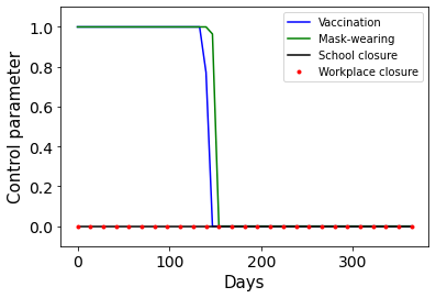
Figure 4: The highest-reward intervention schedule generated by PPO for the SIRV-B environment. Mask-wearing and vaccination are aggressively used until the population is mostly vaccinated.

While SAC performs as well as PPO in SIR-A and SIRV-A, it does not perform as well in the remaining environments. SAC is particularly sensitive to two hyperparameters: reward scale and the update frequency of the neural network. Since we tuned these SAC parameters only on the SIR-A environment, we suspect that each environment may require its own independent hyperparameter tuning. For the epidemic planning problem, this makes PPO a more robust alternative to SAC, one that requires less tuning or no tuning at all. We also note that SAC’s high sample efficiency, when compared to PPO, may not be so important in our application due to the efficiency of the simulator. Finally, we note that training PPO for 30,000 timesteps takes significantly less wall-clock time when compared to SAC (e.g. 3 hours vs. 18 hours on our hardware per training run in C15-B). In critical situations, where policy-makers are exploring multiple different interventions to curb an ongoing epidemic, the time it takes for an RL agent to suggest intervention plans can make or break its integration into their policy-making workflows.

3.2.2 Future Work.

It is important to emphasize that the learned RL policies are heavily influenced by the parameter values that define the disease model (e.g. fatality rate, recovery rate, etc) or the interventions (e.g. the cost of isolation, the effect of masks on transmissibility rate, etc). For example, reducing the cost of workplace closures, or increasing its effectiveness in reducing infectious interactions within workplaces in our benchmark may cause the RL agents to favor this intervention rather than excluding it. Inferring the exact value of these parameters, or calibration, is an active area of research Hazelbag et al. (2020) and  Ritto et al. (2021). Though we consider this to be independent of the optimization problem, it is possible to use our tool to examine the differences in plans sampled from the agent’s policy when the disease has a high versus a low transmissibility rate, or when a vaccine has a high or low efficacy.

We have assumed the availability of a fully observable state in which we know the population size within every compartment. Future work can extend our work to partially observable MDPs where only partial state information is available. Finally, we note that we tuned our hyperparameters on a single configuration; in practice, hyperparameters should be tuned to be robust with respect to a range of parameter settings (e.g. different transition rates).

4 Related Work

Historical Approaches.

Using Markov Decision Processes (MDPs) for epidemic planning was explored as early as 1981 by Lefèvre (1981). Lefèvre (1981) analytically proved that optimal levels of quarantine or medical care are non-decreasing functions of the size of the infectious population. More recently, research on epidemic control has shifted towards a more computational approach where simulations are carefully designed and analyzed to provide insights for epidemic planning. For example, Maharaj and Kleczkowski (2012); Kleczkowski et al. (2012); Oleś et al. (2012), compare, through simulations, many well-established intervention plans.

Our work complements this body of research by demonstrating reinforcement learning as a viable approach to generate alternative candidate strategies that are tailored to a specific environment.

Reinforcement Learning for Epidemic Control.

The COVID pandemic inspired new research into using RL approaches for epidemic control. Among recent works that have formulated different MDPs with actions capturing interventions with the goal of using RL to inform epidemic control, we found Colas et al. (2020); Kompella et al. (2020); Libin et al. (2020) to be the most closely related to our work.

While our motivations are similar, we differ in that we have demonstrated RL as a viable approach to generate intervention plans when there are multiple, continuously-parameterizable interventions that can influence different aspects of the underlying disease and population model. By contrast, Colas et al. (2020); Kompella et al. (2020) combine the effect of many interventions into one that reduces the transmission rate of the disease, thus controlling the disease only via this single parameter. Libin et al. (2020) uses RL to study the cost-effectiveness of different degrees of school closures across regions. In our case, the programmatically-defined interventions can modify any transition rate, and even redistribute the population across disease compartments, regions or facilities. Moreover, as the RL agent can control each intervention independently, it can determine the tradeoffs of different interventions in terms of their costs and benefits — an option that is not possible when grouping multiple interventions into one.

Table 5 provides a feature comparison of the RL approaches used in many of the recent works for epidemic planning.

	$\mathcal{S}$		$\mathcal{A}$
Related Works	C	L	C	L	Sim.
Bastani et al. (2021); Abdallah et al. (2022)	-	-	-	-	-
Libin et al. (2020); Khadilkar et al. (2020) Zong and Luo (2022); Du et al. (2022) Arango and Pelov (2020)	$\bullet$	$\bullet$	-	-	-
Kompella et al. (2020); Colas et al. (2020) Feng et al. (2022b); Bampa et al. (2022) Ohi et al. (2020); Jiang et al. (2020)	$\bullet$	$\bullet$	-	-	$\bullet$
Song et al. (2020)	$\bullet$	$\bullet$	$\bullet$	-	-
Liu (2020)	-	-	$\bullet$	$\bullet$	-
Chadi and Mousannif (2022)	$\bullet$	$\bullet$	-	$\bullet$	-
Kwak et al. (2021); Feng et al. (2022a) Bushaj et al. (2022)	$\bullet$	$\bullet$	-	$\bullet$	$\bullet$
Padmanabhan et al. (2021)	$\bullet$	$\bullet$	$\bullet$	$\bullet$	-
Our Work	$\bullet$	$\bullet$	$\bullet$	$\bullet$	$\bullet$

Table 5: A comparison of recent RL epidemic planning tools in terms of the size of the supported state space $\mathcal{S}$ and action space $\mathcal{A}$ (large (L) $\bullet$  or small/singular -) and their continuity (continuous (C) $\bullet$  or discrete -), and the integration of an epidemic simulator (Sim.) that can simulate different diseases.

5 Conclusions

We present an approach to support public health officials in their efforts to combat epidemics. The approach consists of a reinforcement learning algorithm that proposes policy choices consisting of multiple continuous interventions (e.g., masking, vaccination, isolation, and others, all to various degrees). The ability to model multiple interventions is important, because policy-makers often have multiple strategies available. The ability to model each intervention continuously is important because it is often impractical to impose an intervention absolutely (e.g. critical workers may need to interact with one another). Our tool offers policy-makers quantitatively backed recommendations while leaving to them the final choice of a strategy, which may involve intangibles such as culture or politics.

Our benchmarking environments are similar to real-world epidemic planning environments both in terms of disease models used (SIR, SIRV and C15) and interventions considered. In addition to its application to epidemiology, our work advances reinforcement learning research, through the provision of a realistic benchmarking environment.

Appendix A Appendix

This appendix includes the 15-compartment model used in the C15 benchmarking environments (Figure 5), the RL hyperparameter settings (Table 6), and the highest cumulative reward intervention plans generated by PPO and SAC (Figures 6 and 7).

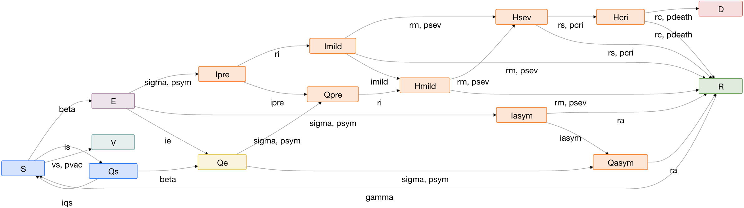
Figure 5: C15: A compartmental model with 15 compartments that affords several interventions such as vaccinations, school and workplace closures.

SAC Hyperparameter	Description	Grid-search values	Chosen value
Reward scale	This is the multiplicative scaling applied after the normalized rewards. It is equivalent to inverse of entropy regularization coefficient	[1, 10, 100, 1000]	100
Learning rate	Learning rate for Adam optimizer, the same learning rate will be used for all networks (Q-Values, Actor and Value function)	[0.003, 0.0003, 0.00003]	0.0003
Training frequency	The number of simulation timesteps to update the model	[5, 25, 125]	5
Learning starts	How many steps of the model to collect transitions for before learning starts	[1000, 5000, 10000]	1000
Batch size	Minibatch size for each gradient update		256
Tau	The soft update coefficient (“Polyak update”, between 0 and 1)		0.005
Gamma	The discount factor		0.99
Buffer size	Size of the replay buffer		1000000
Gradient steps	How many gradient steps to do after each rollout		1
PPO Hyperparameter
Learning rate	The learning rate of the optimizer		0.0003
Num steps	The number of steps to run in each environment per policy rollout		2048
Gamma	The discount factor		0.99
Gae Lambda	The lambda for the general advantage estimation		0.95
Num minibatches	The number of mini-batches		32
Update epochs	The K epochs to update the policy		10
Clip coefficient	The surrogate clipping coefficient		0.2
Entropy coefficient	Coefficient of the entropy		0.0
Vf coefficient	Coefficient of the value function		0.5
Max grad norm	The maximum norm for the gradient clipping		0.5

Table 6: The hyperparameter settings for SAC and PPO.

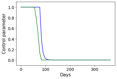
(a) SIR-A

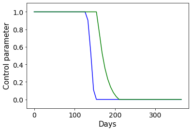
(b) SIRV-A

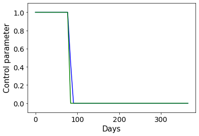
(c) C15-A

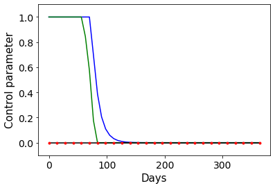
(d) SIR-B

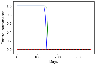
(e) SIRV-B

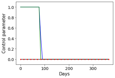
(f) C15-B

Figure 6: Intervention schedules generated by PPO in all 6 environments.

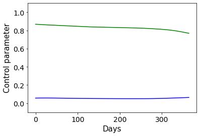
(a) SIR-A

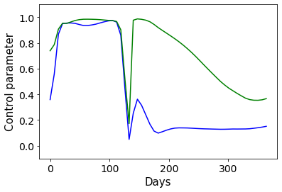
(b) SIRV-A

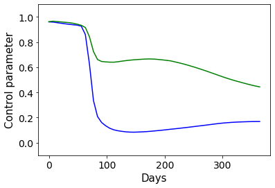
(c) C15-A

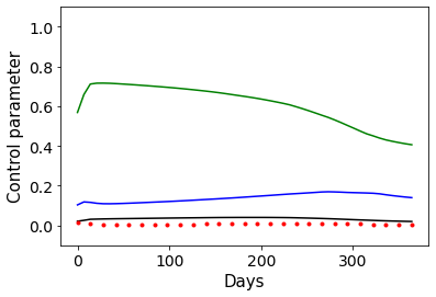
(d) SIR-B

(e) SIRV-B

(f) C15-B

Figure 7: Intervention schedules generated by SAC in all 6 environments

References

- Abdallah et al. [2022] Wejden Abdallah, Dalel Kanzari, Dorsaf Sallami, Kurosh Madani, and Khaled Ghedira. A deep reinforcement learning based decision-making approach for avoiding crowd situation within the case of covid’19 pandemic. Computational Intelligence, 38(2):416–437, 2022.
- Andrychowicz et al. [2020] Marcin Andrychowicz, Anton Raichuk, Piotr Stanczyk, Manu Orsini, Sertan Girgin, Raphaël Marinier, Léonard Hussenot, Matthieu Geist, Olivier Pietquin, Marcin Michalski, Sylvain Gelly, and Olivier Bachem. What matters in on-policy reinforcement learning? A large-scale empirical study. CoRR, abs/2006.05990, 2020.
- Arango and Pelov [2020] Mauricio Arango and Lyudmil Pelov. Covid-19 pandemic cyclic lockdown optimization using reinforcement learning. arXiv preprint arXiv:2009.04647, 2020.
- Bampa et al. [2022] Maria Bampa, Tobias Fasth, Sindri Magnusson, and Panagiotis Papapetrou. : Learning intervention strategies for epidemics with reinforcement learning. In International Conference on Artificial Intelligence in Medicine, pages 189–199. Springer, 2022.
- Barlow and Weinstein [2020] N. S. Barlow and S. J. Weinstein. Accurate closed-form solution of the SIR epidemic model. Physica D, 408:132540, Jul 2020.
- Bastani et al. [2021] Hamsa Bastani, Kimon Drakopoulos, Vishal Gupta, Ioannis Vlachogiannis, Christos Hadjichristodoulou, Pagona Lagiou, Gkikas Magiorkinis, Dimitrios Paraskevis, and Sotirios Tsiodras. Efficient and targeted covid-19 border testing via reinforcement learning. Nature, 599(7883):108–113, 2021.
- Bushaj et al. [2022] Sabah Bushaj, Xuecheng Yin, Arjeta Beqiri, Donald Andrews, and İ Esra Büyüktahtakın. A simulation-deep reinforcement learning (sirl) approach for epidemic control optimization. Annals of Operations Research, pages 1–33, 2022.