Tomography of a solar plage with the Tenerife Inversion Code

Abstract

We apply the Tenerife Inversion Code (TIC) to the plage spectropolarimetric observations obtained by the Chromospheric LAyer SpectroPolarimeter (CLASP2). These unprecedented data consist of full Stokes profiles in the spectral region around the Mg II h and k lines for a single slit position, with around two thirds of the 200 arcsec slit crossing a plage region and the rest crossing an enhanced network. A former analysis of these data had allowed us to infer the longitudinal component of the magnetic field by applying the weak field approximation (WFA) to the circular polarization profiles, and to assign the inferred magnetic fields to different layers of the solar atmosphere based on the results of previous theoretical radiative transfer investigations. In this work, we apply the recently developed TIC to the same data. We obtain the stratified model atmosphere that fits the intensity and circular polarization profiles at each position along the spectrograph slit and we compare our results for the longitudinal component of the magnetic field with the previously obtained WFA results, highlighting the generally good agreement in spite of the fact that the WFA is known to produce an underestimation when applied to the outer lobes of the Mg II h and k circular polarization profiles. Finally, we use the inverted model atmospheres to give a rough estimation of the energy that could be carried by Alfvén waves propagating along the chromosphere in the plage and network regions, showing that it is sufficient to compensate the estimated energy losses in the chromosphere of solar active regions.

1 Introduction

One of the major challenges in solar physics is the determination of the magnetic field vector in the solar chromosphere (e.g., the review by Trujillo Bueno & del Pino Alemán, 2022), which in turn is key to understanding the physics of this interface region between the underlying photosphere and the overlying corona. In the chromosphere the magnetic pressure starts to overcome the gas pressure and the magnetic field increasingly dominates the plasma dynamics and structure (e.g., the review by Carlsson et al., 2019, and references therein).

Most of the spectral lines that form in the upper solar chromosphere and in the transition region up to the million-degree corona are resonance lines in the ultraviolet (UV), a spectral region not accessible by ground based facilities. The polarization signals of UV spectral lines encode information about the plasma magnetic field in such key regions of the solar upper atmosphere (Trujillo Bueno et al., 2017).

Motivated by theoretical investigations of the polarization in the Mg II h-k doublet around 280 nm (Belluzzi & Trujillo Bueno, 2012), the CLASP2 (Chromospheric LAyer SpectroPolarimeter; Narukage et al., 2016) suborbital space experiment was performed in 2019, allowing the observation of the intensity and polarization in this near-UV region of the spectrum in both a quiet Sun region near the limb (Rachmeler et al., 2022) and in an active region plage (Ishikawa et al., 2021). The CLASP2 mission was a true success and it achieved unprecedented observations of the UV solar spectrum between approximately 279.30 and 280.68 nm, which includes the Mg II h and k resonance lines and the three resonance lines of Mn I at 279.56, 279.91, and 280.19 nm.

The observations corresponding to the plage region showed fractional circular polarization signals of significant amplitude in the above-mentioned Mg II and Mn I spectral lines. A first analysis of these data enabled an estimate of the longitudinal component of the magnetic field by applying the weak field approximation (WFA) to the intensity and circular polarization profiles (Ishikawa et al., 2021). Based on theoretical radiative transfer investigations, the magnetic field strengths inferred from the Mg II h-k doublet (del Pino Alemán et al., 2020; Afonso Delgado et al., 2023) and Mn I triplet (del Pino Alemán et al., 2022) were assigned to different layers of the solar atmosphere. In particular, the Mg II lines provided the longitudinal component of the magnetic field in the upper and middle chromosphere, while the Mn I lines provided it in the lower chromosphere. Together with the simultaneous observations carried out by HINODE/SOT-SP in photospheric lines, this resulted in a map of the magnetic field (its longitudinal component) from the photosphere to the base of the corona (Ishikawa et al., 2021).

Recently, Li et al. (2022) developed the Tenerife Inversion Code (TIC), a non-LTE inversion code of Stokes profiles produced by the scattering of anisotropic radiation and the Hanle and Zeeman effects in spectral lines. The TIC takes into account the effects of radiative transfer in one-dimensional models of the solar atmosphere, as well as the effects of partial frequency redistribution and $J$-state interference (necessary to model the Mg II h-k doublet) and of the radiation field anisotropy (which has a significant impact even on the circular polarization of the Mg II h-k doublet; Alsina Ballester et al. 2016; del Pino Alemán et al. 2016; Li et al. 2022). The TIC can be applied to a variety of spectropolarimetric observations in order to get the stratification of the magnetic field in the observed region, including the spectropolarimetric data of the Mg II h and k lines obtained by CLASP2.

In this work, we apply TIC to the Stokes $I$ and $V$ profiles of the Mg II h and k lines and of the two blended lines of the Mg II subordinate triplet at $279.88$ nm observed by CLASP2 in an active region plage. The Stokes Q and U signals were also successfully measured by CLASP2 in the observed active region plage (see figure S2 of Ishikawa et al., 2021) and in the observed quiet region close to the limb (see figure 2 of Rachmeler et al., 2022 and figure 6 of Trujillo Bueno & del Pino Alemán, 2022), however, the inversion of the four Stokes parameters is significantly more complex, both in terms of computational time and from the physics involved in the scattering problem, and therefore is left for a future investigation. In Section 2 we briefly describe the most relevant aspects of the data as well as our inversion strategy. In Section 3 we show the results of the inversion. We compare the resulting longitudinal component of the magnetic field with the WFA inference by Ishikawa et al. (2021). We then use the inverted model atmosphere in order to estimate the energy flux that could be carried by Alfvén waves propagating through the chromospheres of plage and network regions. Finally, we summarize our conclusions in Section 4.

2 Observations and inversion strategy

In this section we summarize the main characteristics of the observations and describe the inversion strategy we have applied with the TIC.

2.1 Observation

The subject data of this work was obtained by the CLASP2 launched by a NASA sounding rocket on 11 April 2019. In particular, here we focus on the data corresponding to the plage target. The first analysis of this data was carried out by Ishikawa et al. (2021), who applied the WFA to the intensity and circular polarization profiles of the Mg II h-k doublet and Mn I lines at $279.91$ and $280.19$ nm to infer the longitudinal component of the magnetic field in different layers of the solar atmosphere.

The data used in this work are the Stokes $I$ and $V$ profiles at each point of the 196 arcsec slit of the spectrograph covering an active region plage and its surrounding enhanced network at the East side of NOAA 12738 (see panel C of Fig. 1). The data was recorded between 16:53:40 and 16:56:16 UT. ($\approx 2.5$ min). The spectral range covers from 279.30 to 280.68 nm with a spectral sampling of 49.9 mÅ/pixel. The instrument’s spectral profile can be approximated with a Gaussian with a full width at half maximum (FWHM) of 110 m$\rm\AA$, which results from the convolution of the spectrograph’s slit with the spectral point spread function (PSF; Song et al., 2018; Tsuzuki et al., 2020). The spectral resolution of the data is, therefore, about 28000. The Mg II h and k lines at 279.6 and 280.3 nm, respectively, as well as the two subordinate lines at 279.88 nm (they are blended), are found in this spectral range.

The Stokes profiles of the Mg II h-k doublet show sizable circular polarization in the bright plage and weaker circulation polarization in the enhanced network region, from which we can infer the longitudinal component of the magnetic field in the solar chromosphere.

2.2 Inversion strategy

We apply TIC in order to infer the stratification of the thermodynamical parameters—namely temperature ($T$), gas pressure ($P_{\rm g}$), microturbulent velocity ($v_{\rm turb}$), the vertical component of the macroscopic velocity ($v_{z}$), and the vertical component of the magnetic field ($B_{z}$) —in the solar plage target observed by the CLASP2. TIC is based on the HanleRT forward engine (del Pino Alemán et al., 2016, 2020), which implements the coherent scattering formalism of Casini et al. (2014, 2017a, 2017b). At each pixel along the spatial direction of the spectrograph’s slit we invert the observed Stokes profiles, after temporally co-adding the data to attain a suitable signal to noise ratio for the inversion.

We use a 6-levels atomic model (5 Mg II levels and the Mg III ground level), including the h-k doublet and the subordinate lines in the observed range (see also del Pino Alemán et al., 2020). The stratification in the model atmosphere is sampled with 60 nodes between ${\rm log_{10}}(\tau_{500})=-8$ and 1. The nodes are not equally spaced in order to refine the sampling between ${\rm log_{10}}(\tau_{500})=-6.5$ and -3, which corresponds to the region of formation of the Mg II h and k lines. We invert the Stokes profiles in 5 cycles:

• Invert $T$, $v_{\rm turb}$, and $v_{z}$ with 4, 2, and 3 nodes, respectively, using only the intensity profile. The initial model atmosphere is the static model C of Fontenla et al. (1993).

• Invert $T$, $v_{\rm turb}$, and $v_{z}$ with 7, 4, and 5 nodes, respectively, using only the intensity profile.

• Invert $B_{z}$ with 1 node, using both Stokes I and V, and neglecting the anisotropy of the radiation field.

• Invert $T$, $v_{\rm turb}$, $v_{z}$, and $B_{z}$ with 7, 4, 5, and 5 nodes, respectively, using both Stokes I and V, and neglecting the anisotropy of the radiation field.

• Invert $B_{z}$ with 5 nodes, using both Stokes I and V, and taking into account the radiation field anisotropy.

Every cycle after the first is initialized from the model atmosphere resulting from the previous cycle. The first two cycles results in the model atmosphere that fits the intensity profile observed at the spatial pixel under consideration, and they are relatively fast because polarization is not taken into account. Note that because we assume hydrostatic equilibrium, $P_{\rm g}$ is fully determined by its value at the top boundary and the temperature stratification. Whenever the thermodynamic variables are being inverted, the boundary value of $P_{\rm g}$ also is. The second cycle is more time consuming due to the increased number of nodes, but can provide added complexity (if needed) to the stratification of thermodynamic parameters. The radiation field anisotropy has a significant impact on the circular polarization of the Mg II h-k doublet (Alsina Ballester et al., 2016; del Pino Alemán et al., 2016; Li et al., 2022) and it is necessary to take it into account. However, accounting for the anisotropy makes the inversion appreciably slower. For this reason the first two magnetic cycles (3 and 4) neglect this contribution. The relatively fast third cycle gives a very rough estimation of $B_{z}$, and then the fourth cycle adds stratification to $B_{z}$ while also letting the thermodynamic parameters slightly change to improve the simultaneous fit of both intensity and circular polarization. Finally, in the fifth cycle the radiation field anisotropy is included and $B_{z}$ is readjusted.

It is important to clarify that the line of sight (LOS) is not at the disk center (it varies from $\mu\approx 0.65$ to $\mu\approx 0.85$ along the slit). When including the radiation field anisotropy, the geometry with respect to the propagation directions of the radiation within the atmosphere is important, and not just along the LOS. If the macroscopic velocity or the magnetic field vector are not vertical, the forward problem is no longer axially symmetric and the computing time is significantly increased. This is the reason why the inversion is on $v_{z}$ and $B_{z}$. These vertical components are then projected onto the LOS, and thus we plot the result for the velocity longitudinal component ($v_{\rm\parallel}$) and the magnetic field longitudinal component ($B_{\rm\parallel}$). In the inversions shown in this work we assume that a single magnetic field fills the whole pixel (i.e., we assume the magnetic filling factor to be unity).

3 Results

In this section we show the results of the inversion of the intensity and circular polarization profiles obtained by the CLASP2 in the observed active region plage (see Section 2.1). We compare our results with those of Ishikawa et al. (2021), which inferred $B_{\rm\parallel}$ at different heights in the solar atmosphere by applying the WFA. Finally, we use the inferred atmospheric parameters to estimate the sound speed, the Alfvén velocity, the plasma $\beta$ parameter, as well as the energy flux of Alfvén waves.

3.1 Inverted model atmosphere

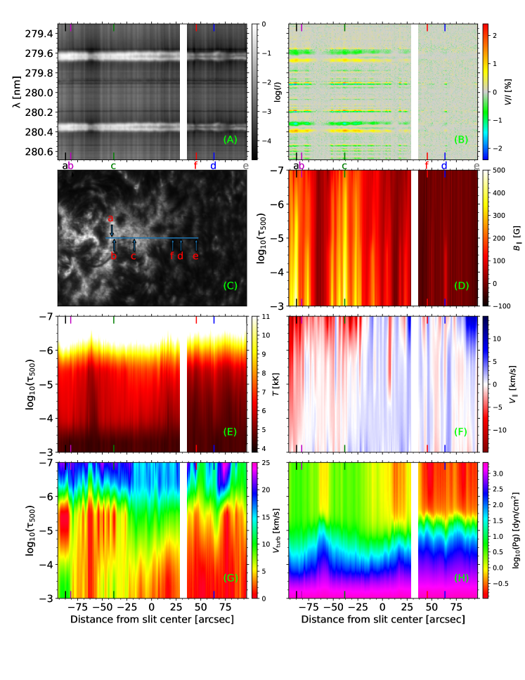
Figure 1: Intensity profiles (panel A) normalized to the maximum, in log scale, and fractional circular polarization $V/I$ profiles (panel B), measured by CLASP2. Panel (C): slit-jaw image of Lyman$-\alpha$ recorded by CLASP2. The blue line denotes the location of the spectrograph’s slit. Panels D to H show the results for $B_{\rm\parallel}$, $T$, $v_{\rm\parallel}$, $v_{\rm turb}$, and $P_{\rm g}$, respectively. The a, b, c, d, e, and f labels indicate the locations of the profiles shown in Fig. 2.

Following the strategy in Section 2.2, we apply the TIC code to the Stokes profiles for each slit position of the CLASP2 plage target observation (Section 2.1). The inversion results are shown in Fig. 1.

The intensity shows the typical two-peaks profiles and they are brighter inside the plage (located approximately between slit positions at -95 and 28 arcsec) than in the surrounding enhanced network regions (see panel A of Fig. 1). The white vertical band at around 34 arcsec corresponds to the lack of data due to dust in the instrument. It is well known that the h and k line centers (often dubbed h₃ and k₃, respectively) form in the upper chromosphere, while the peaks (dubbed h_2v and h_2r, for the h line, and k_2v and k_2r for the k line) form in the middle chromosphere, and the minima outside the peaks (dubbed h₁ and k₁, respectively) form close to the temperature minimum of standard semi-empirical models (Vernazza et al., 1981). The Mg II h and k lines are thus sensitive to a relatively wide range of heights through the solar chromosphere.

The $V/I$ profiles are shown in panel B. These signals are the strongest inside the plage region, as expected, resulting in larger $B_{\rm\parallel}$. In this region, the strengths of the magnetic flux concentrations reach around $300$ G in the upper chromosphere (from ${\rm log_{10}}(\tau_{500})\approx-5.5$ to $\approx-6.5$, see panel D of Fig. 1). The plage region also shows higher temperatures at chromospheric heights (from ${\rm log_{10}}(\tau_{500})\approx-3.5$ to $\approx-6.0$) with respect to the surrounding enhanced network region (see panel E of Fig. 1).

The $v_{\rm\parallel}$ macroscopic velocity gradients are necessary to get the observed asymmetries between k_2v and k_2r, and equivalently for the h line (Leenaarts et al., 2013), as can be seen in panel F of Fig. 1. The inverted macroscopic velocity is mostly downward (red color in the figure) at the slit positions between approximately -95 and -25 arcsec, while mostly upward (blue color in the figure) between approximately -25 and 30 arcsec.

The $v_{\rm turb}$ parameter accounts mainly for the missing broadening due to the three-dimensional plasma dynamics. We get relatively small values up to the mid chromosphere (${\rm log_{10}}(\tau_{500})\approx-5.8$) in most of the slit, significantly increasing in the upper chromosphere (see panel G of Fig. 1). Generally, $v_{\rm turb}$ is larger in the bright plage region.

The stratification of $P_{\rm g}$ is calculated assuming hydrostatic equilibrium (e.g., Mihalas, 1970), although its value in the upper boundary is allowed to change in the inversion (see panel H of Fig. 1). The electron and hydrogen number densities are computed in the forward solver by assuming LTE and solving the equation of state with the method of Wittmann (1974).

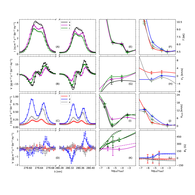
Figure 2: Observed (open circles) and fit (solid curves) profiles (A, B, C, and D) for the intensity (A and C) and circular polarization (B and D) at the slit locations indicated in Fig. 1 in the plage (panels A and B; locations a, b, and c) and in the enhanced network and quiet sun (panels C and D; locations d and e and f, respectively). The two left columns show the k and h lines. The error bars in the circular polarization profiles indicate the photon noise. Fit profiles with the full spectral range, including the subordinate lines, are shown in Fig. A.1 for the plage (b) and enhanced network (d) slit locations. The two right columns show, from top to bottom, the inverted T (E, F), $v_{\rm\parallel}$ (G, H), $v_{\rm turb}$ (I, J), and $B_{\rm\parallel}$ (K, L) stratification, with the color of each curve corresponding to a slit position as indicated in the legends in panels A and C. In panels K and L, the solid (dashed) curves show the result from the fifth (fourth) inversion cycle, that is, including (neglecting) the radiation field anisotropy (see Section 2.2).

The labels a, b, c, d, e, and f in Fig. 1 indicate the slit position of the six profiles shown in Fig. 2, each profile plotted using the same color as the corresponding label. The profiles at locations b, c, and d are also shown in Ishikawa et al. (2021). The profiles in panels (A) and (B) in Fig. 2 (a,b, and c) are located in the plage region, while those in (C) and (D) are located in the enhanced network (d and e) and quiet Sun (f) regions.

The intensity profiles corresponding to the plage (panel A of Fig. 2) are significantly brighter and show a relatively shallow central trough compared to the profiles outside the plage (panel C). Regarding the circular polarization profiles, the ones in the plage (panel B of Fig. 2) show the typical spectral shape with four lobes, while those outside the plage show significantly depressed inner lobes which are almost absent.

The inverted model atmospheres in the plage region are similar to those inferred by de la Cruz Rodríguez et al. (2016), showing higher temperature (panel E of Fig. 1 and Fig. 2) and gas pressure (panel H of Fig. 1) compared to the region outside the plage. Moreover, the temperature in the lower chromosphere (from ${\rm log_{10}}(\tau_{500})\approx-4$ to $\approx-5.3$) increases to more than $6000$ K, a temperature enhancement when compared to the models from outside the plage. A similar result was found by Carlsson et al. (2015), who introduced a chromospheric plateau of about $6500$ K in model P of Fontenla et al. (1993) to be able to fit some plage observations of the Mg II h and k lines from the Interface Region Imaging Spectrograph (IRIS; De Pontieu et al., 2014).

The three selected plage profiles have k${}_{2v}>$ k_2r and h${}_{2v}>$ h_2r, which is associated with negative velocity gradients in the middle and upper chromosphere (i.e., macroscopic velocity decreasing with height; see also Leenaarts et al., 2013; Afonso Delgado et al., 2023). The inverted $v_{\rm\parallel}$ (panel G of Fig. 2) confirms this expected behavior. On the contrary, the profile at location e (see the gray curves in panel C of Fig. 2) has k${}_{2r}>$ k_2v and h${}_{2r}>$ h_2v, indicative of positive velocity gradients, as recovered by the inversion (gray curve in panel H of Fig. 2).

A larger $v_{\rm turb}$ in the lower chromosphere is necessary to fit the relatively broad wings close to the k₃ and h₃ (compared to the rest of the selected profiles) of the plage profiles at locations a and c (panel I of Fig. 2). The narrower peak separations in these two profiles (a and c) result, in turn, in smaller $v_{\rm turb}$ in the middle chromosphere with respect to the other four selected profiles.

Finally, we show the inverted $B_{\rm\parallel}$ in panels K and L of Fig. 2, which correspond to slit positions inside and outside the bright region of the observed plage, respectively. The solid curves show the result of the inversion taking into account the impact of radiation anisotropy (fifth inversion cycle), while the dashed curves show the result of the inversion by neglecting it (fourth inversion cycle). Neglecting the impact of radiation anisotropy results in the retrieval of larger magnetic fields in the plage region, as explained in Li et al. (2022). Although the anisotropy only impacts the outer lobes, and thus we should expect this difference to appear just in the lower chromosphere, we see an effect on the inverted $B_{\rm\parallel}$ in the upper chromosphere due to the coupling induced by the spectral point spread function (PSF) (Centeno et al., 2022).

In the three plage locations (a, b, and c) we get $B_{\rm\parallel}$ of up to $300$ G in the middle chromosphere, decreasing with height. This magnetic field strength is of similar order to those reported by Morosin et al. (2020) and Pietrow et al. (2020) in plage regions, obtained from the inversion of spectropolarimetric data in the Ca II line at $854.2$ nm. In the enhanced network position (d) $B_{\rm\parallel}$ is about $88$ G at ${\rm log_{10}}(\tau_{500})=-4.38$, around $10$% larger than what was estimated by Ishikawa et al. (2021) by applying the WFA to the outer lobes of the h line circular polarization profile. Note that the application of the WFA to the outer lobes of the Mg II h-k doublet circular polarization profiles generally underestimates $B_{\rm\parallel}$ and that this error is of the order of $10$% for the h line (Ishikawa et al., 2021). For this enhanced network location the magnetic field in the upper chromosphere is close to zero, as expected from the very small inner lobes in the circular polarization profile. The fit to these profiles (locations f and e) are worse. In these quieter regions of the Sun we expect magnetic concentration of smaller scale (Stenflo, 1989) and, thus, not only the magnetic field is probably not filling the full pixel of the observation, but several different longitudinal magnetic fields can coexist in each pixel leading to significant signal cancellation.

3.2 Comparison with previous results

Ishikawa et al. (2021) first analyzed the data used in this work by applying the WFA to infer $B_{\rm\parallel}$ at different heights in the solar atmosphere. The discrete heights of the $B_{\rm\parallel}$ values inferred via the WFA are only approximate, with the locations along the LOS based on theoretical investigations (Afonso Delgado et al., 2023; del Pino Alemán et al., 2022). In this work we have instead applied an inversion code and we are thus able to infer the whole stratification of those regions contributing to the formation of the emergent Stokes parameters. Despite these differences, it is valuable to compare the two results and to determine the degree of agreement between them.

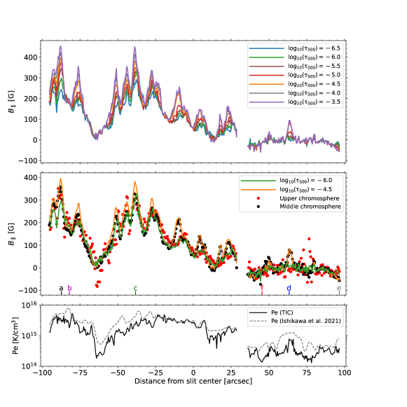
Figure 3: Upper panel: inverted $B_{\rm\parallel}$ at ${\rm log_{10}}(\tau_{500})=-6.5,-6.0,-5.5,-5.0,-4.5,-4.0$, and $-3.5$ (solid curves, see legend) for each slit position. Middle panel: inverted $B_{\rm\parallel}$ at ${\rm log_{10}}(\tau_{500})=-6.0$ and $-4.5$. The filled circles show the $B_{\rm\parallel}$ in Fig. 3 of Ishikawa et al. (2021), with the same color legend, namely, red for upper chromosphere and black for middle chromosphere. Bottom panel: the black solid curve shows the inverted electron pressure at ${\rm log_{10}}(\tau_{500})=-5.4$ (see right axis) for each slit position. The gray dashed curve shows the electron pressure at ${\rm log_{10}}(\tau_{500})=-5.4$ from Ishikawa et al. (2021).

In the upper panel of Fig. 3, we show the inferred $B_{\rm\parallel}$ at every position of the slit at various heights. The $B_{\rm\parallel}$ values in the lower chromosphere ($\sim$${\rm log_{10}}(\tau_{500})=-4.0$) and at the temperature minimum ($\sim$${\rm log_{10}}(\tau_{500})=-3.5$) are somewhat smaller than those inferred from the Mn I lines in Ishikawa et al. (2021). This is due to the lack of sensitivity of the Mg II lines to these layers of the model atmosphere. In order to get a more reliable $B_{\rm\parallel}$ estimation in the region just above the temperature minimum using the CLASP2 data, we should include the inversion of the Mn I lines. This, however, is currently beyond the capabilities of TIC, as it requires to take into account the hyperfine structure of Mn I (del Pino Alemán et al., 2022). The inverted $B_{\rm\parallel}$ are similar to the results of Ishikawa et al. (2021) for the middle and upper chromosphere. Because the particular height that should be assigned to the $B_{\rm\parallel}$ retrieved by applying the WFA depends on the particular stratification of the atmosphere and the source function for the circular polarization, we cannot expect to find a particular optical depth that perfectly matches the WFA inference everywhere. Nevertheless, we can see that the $B_{\rm\parallel}$ values inferred for the middle chromosphere in are mostly between our ${\rm log_{10}}(\tau_{500})=-4.5$ and $-5.0$ values, and that those for the upper chromosphere are mostly between our ${\rm log_{10}}(\tau_{500})=-5.5$ and $-6.0$ values. We note that the two inferences agree within the error bars shown in Ishikawa et al. (2021) and in our Fig 2.

The black solid curve in the bottom panel of Fig. 3 shows the TIC-inferred electron pressure, i.e., the product of the temperature and the electron density, at ${\rm log_{10}}(\tau_{500})=-5.4$. The gray dashed curve shows the electron pressure obtained by Ishikawa et al. (2021) at the same optical depth inverted with IRIS² (Sainz Dalda et al., 2019). While the overall trend is similar, the two determinations of electron pressure show clear differences. This is to be expected, since both codes only invert for the electron density at the top boundary, while the stratification of this quantity relies on the assumption of hydrostatic equilibrium, and the treatment of the equation of state by the two codes is different. However, both inversions demonstrate that the electron pressure correlates with the inverted $B_{\rm\parallel}$, supporting the magnetic origin of the upper-chromosphere heating above active region plages. In particular, the TIC inversion gives Pearson correlation coefficients of 0.92, 0.68, and 0.74 between $B_{\rm\parallel}$ and $P_{\rm e}$ at ${\rm log_{10}}(\tau_{500})=-6.0$, $-5.4$, and $-5.0$, respectively.

In conclusion, our results on the stratification of $B_{\rm\parallel}$ obtained by applying TIC to the CLASP2 plage data agree with the results of Ishikawa et al. (2021), obtained by applying the WFA to the same data, and assigning the inferred value of $B_{\rm\parallel}$ to regions in the solar atmosphere based on theoretical studies of the formation of the Mg II h-k doublet.

3.3 Magnetic energy in the plage chromosphere

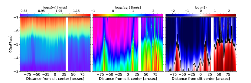
Figure 4: Speed of sound (left panel), Alfvén velocity (middle panel), and ratio between gas pressure and the magnetic pressure (right panel), with the black solid curve indicating where this ratio is unity. The two middle and right panels assume that the field is fully longitudinal, i.e., $B=$$B_{\rm\parallel}$

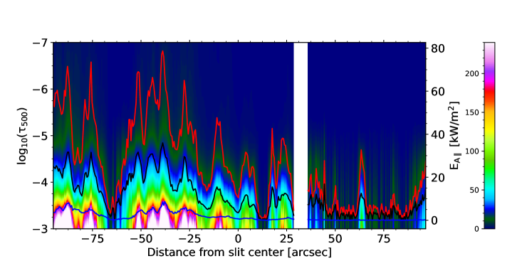
Figure 5: Energy flux of Alfvén waves by assuming that the magnetic field is fully given by $B_{\rm\parallel}$and that the velocity amplitude is $v=2$ km/s. The red, black, and blue curves denote the energy flux at ${\rm log_{10}}(\tau_{500})=-4.0,-4.5$, and $-5.8$, respectively.

We used the inferred model atmosphere described in the previous sections to estimate the speed of sound ($v_{s}=\sqrt{\gamma P_{\rm g}/\rho}$, where $\gamma$ is the adiabatic index that we take as $\gamma=5/3$ and $\rho$ is the density) and the Alfvén velocity (under the assumption that the magnetic field is fully directed along the LOS; $v_{A}=\sqrt{B^{2}_{\parallel}/(\mu_{0}\rho)}$, in SI units, Priest 2014, where $\mu_{0}$ is the vacuum permeability) in the chromosphere of the observed plage region. We show these two quantities in the left and middle panels of Fig. 4, respectively. The right panel shows the plasma $\beta=2\mu_{0}P_{g}/B^{2}$—i.e., the ratio between the gas and magnetic pressures—assuming that the magnetic field is fully along the LOS (i.e., $B=B_{\parallel}$). The $\beta=1$ surface is indicated by the black curve in the corresponding panel. Around the slit positions at $-90$, $-75$, $-40$, and $-25$  arcsec the magnetic pressure has overcome the gas pressure ($\beta<1$) already at ${\rm log_{10}}(\tau_{500})=-3$. In the rest of the plage, we find $\beta=1$ in the lower chromosphere, except around the slit position around $-60$ arcsec, where the magnetic field drops to very small values, and close to the border of the plage region around the slit position at $10$ arcsec. Outside of the plage, the $\beta=1$ surface is in the middle chromosphere instead, except in the enhanced network region where the $\beta=1$ surface is lower than in the surrounding quiet regions. The shape of the $\beta=1$ surface inside of the plage resembles that of upside-down “cones”, what may be indicative of magnetic flux concentrations expanding with “height”.

Several different mechanisms have been proposed for the heating of the chromosphere above plages, e.g., magneto-acoustic shocks, Alfvén waves, magnetic reconnection, and Ohmic dissipation (e.g., Carlsson et al., 2019; Anan et al., 2021). Certainly, the strong correlation between the inferred $B_{\rm\parallel}$ and the electron pressure discussed in the previous section supports the hypothesis that chromospheric heating above plages is of magnetic origin. In particular, Alfvén waves have been considered to play an important role in chromospheric heating and they have been observed in chromospheric structures (De Pontieu et al. 2007; Jess et al. 2009, 2015; Grant et al. 2018, and Van Doorsselaere et al. 2020). From magneto-hydrodynamic (MHD) simulations, van Ballegooijen et al. (2011) pose that Alfvén waves produced by the motion of the footpoint of a flux tube can be reflected due to the steep increase of the Alfvén speed with height. The interaction between the counterpropagating waves lead to the Alfvén wave turbulence and dissipation in the chromosphere. Soler et al. (2017) studied the propagation of torsional Alfvén waves in expanding flux tubes, finding that only the lower frequency waves are reflected, while the high frequency ones are damped in the chromosphere by ion-neutral collisions, with only the intermediate frequency waves being transmitted into the corona. Our inversion results show significant $v_{\rm turb}$ in the lower chromosphere of the plage region (see panel G of Fig. 1 and curves a and c in panel G of Fig. 2), in agreement with the inversions of de la Cruz Rodríguez et al. (2016) in IRIS observations. $v_{\rm turb}$ accounts for many broadening contributions that cannot be accounted for in 1D radiative transfer modeling. Therefore, it is not possible to establish a direct relation between the increased $v_{\rm turb}$ in the plage region inversion with the presence of this Alfvén wave turbulence. Nevertheless, it is worth noting that it is a plausible explanation of the results.

The total duration of the CLASP2 observation is too short for investigating whether or not the observed Stokes profiles show any hint of Alfvén waves. However, torsional Alfvén waves have been observed in the network with velocity amplitudes of $2.6$ km/s (e.g., Jess et al., 2009). By assuming that Alfvén waves do exist in the observed plage region and that their amplitude is about $v=2$ km/s we can have a rough estimation of the energy flux carried by Alfvén waves ($E_{A}$), also assuming that the magnetic field is fully given by $B_{\rm\parallel}$($E_{A}=\rho v^{2}v_{A}$).

In Fig. 5 we show this rough estimate of the energy flux that could be carried by Alfvén waves, with the red, black, and blue curves showing the energy flux (right axis of the figure) corresponding to ${\rm log_{10}}(\tau_{500})=-4.0$, $-4.5$, and $-5.8$, respectively. At ${\rm log_{10}}(\tau_{500})=-4.0$ the energy flux can reach 60 kW/m² inside the plage, while it is around 30 kW/m² in the network. This value is of similar order than the energy loss estimated by Withbroe & Noyes (1977; $2\cdot 10^{7}$ erg/cm²/s, i.e. $20$ kW/m²) and by Morosin et al. (2022; $26.1$ kW/m²) in the chromosphere of active regions. At ${\rm log_{10}}(\tau_{500})=-4.5$ the energy flux would be around $30$ kW/m² in the plage and around $10$ kW/m² in the network. Therefore, Alfvén waves with a velocity amplitude of $2$ km/s could carry enough energy to balance out the energy losses in the chromosphere in the plage region. It is important to take into account that we are assuming that the magnetic field strength is given by $B_{\rm\parallel}$, and this is a lower limit of the actual field strength. Therefore, Alfvén amplitudes even smaller than $2$ km/s may already be sufficient to reach this energy flux.

4 Summary and discussion

We have applied the TIC to the intensity and circular polarization profiles observed by the CLASP2 in an active region plage and enhanced network regions, obtaining the stratification of the temperature (T), line of sight velocity ($v_{\rm\parallel}$), microturbulent velocity ($v_{\rm turb}$), gas pressure ($P_{\rm g}$), and the longitudinal component of the magnetic field ($B_{\rm\parallel}$) at each position along the spectrograph slit. In the inversion we have fit the intensity and circular polarization profiles of the Mg II h-k doublet and subordinate triplet at 279.88 nm. The general properties of the atmospheric models obtained are in agreement with the results presented in previous works. The inverted plage models show larger temperature and gas pressure, similar to those obtained by de la Cruz Rodríguez et al. (2016) for a plage observation from IRIS. Likewise, the plage models obtained show a plateau-like region in the temperature stratification with values around 6500 K, which is the same temperature of the plateau that Carlsson et al. (2015) added to the P model of Fontenla et al. (1993) in order to fit some plage observations from IRIS.

The longitudinal magnetic field that results from the inversion is in agreement with the WFA inference by Ishikawa et al. (2021) for the middle and upper chromosphere, especially when taking into account that the application of the WFA to the wings of the Mg II h line systematically underestimates the magnetic field by about 10%. Our inversions retrieve smaller $B_{\rm\parallel}$in the lower chromosphere when compared with the results of Ishikawa et al. (2021). However, this may be due to a lack of sensitivity to those layers of the atmosphere (see the circular polarization response function in Fig. 3 of del Pino Alemán et al. 2022). The inversion at these atmospheric layers could be significantly improved by including the Mn I lines, however, being Mn I a minority species (which usually entails relatively large atomic models to correctly model their spectral lines) and the need to account for hyperfine structure (especially to correctly model their circular polarization profiles) would entail a prohibitive increase of the required computing time.

In the upper chromosphere, the electron pressure derived with TIC is not identical to that shown in Ishikawa et al. (2021) derived with IRIS². However, this is expected considering the different treatment of the equation of state by the two codes. Nevertheless, what is really important is that there is agreement in the correlation between the electron pressure and the $B_{\rm\parallel}$, which strongly supports the magnetic origin of the heating of the upper chromosphere.

From the inverted model atmospheres we have estimated the Alfvén velocity and the plasma $\beta$ under the assumption that the magnetic field is fully given by $B_{\rm\parallel}$. The shape of the $\beta=1$ surface in the plage, namely, that of inverted “cones”, may be indicative of magnetic flux concentrations expanding with height. We need to take into consideration, however, that our inversions are in optical depth scale, and two positions at the same optical depth in two different columns are not necessarily one next to the other in geometrical scale. Nevertheless, if the thermodynamic quantities are similar between neighbor columns, we can expect adjacent points in optical depth to be relatively close in geometrical height as well.

Finally, by assuming a velocity amplitude for Alfvén waves of $2$ km/s, based on the previous results in the literature (Jess et al., 2009), we have estimated the energy flux carried by Alfvén waves in the inferred model atmosphere. The energy flux inside the plage at the middle chromosphere (${\rm log_{10}}(\tau_{500})=-4.5$) is about 30 kW/m², of similar order as the energy loss of $20$ kW/m² in the chromosphere of active regions estimated by Withbroe & Noyes (1977). At ${\rm log_{10}}(\tau_{500})=-4.0$, this energy flux reaches 60 kW/m². Consequently, Alfvén waves with a velocity amplitude of $2$ km/s could carry enough energy to balance out the energy losses in the chromosphere of the plage region. Moreover, our assumption of the magnetic field strength being given uniquely by $B_{\rm\parallel}$ can only be a lower limit of the actual field strength and, therefore, smaller velocity amplitudes may be sufficient in order to reach these energy fluxes.

As shown in this paper, the TIC is a very useful plasma diagnostic tool for inferring the magnetic, thermodynamic and dynamic properties of the solar chromosphere from spectropolarimetric observations of the resonance lines, such as the Mg II h and k doublet, that the CLASP2 suborbital space experiment has made possible. We therefore believe that the diagnostic capabilities of the scientific community are ready to be applied to a mission dedicated to these observables, and that the development of a space telescope equipped with instruments like CLASP2 would lead to a revolution in our empirical understanding of the magnetic field in the solar upper atmosphere.

Appendix A fit profiles for the whole spectral range

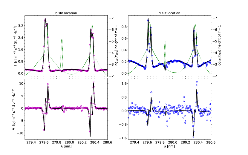
Figure A.1: Observed (open circles) and fit (solid curves) intensity (top panels) and circular polarization (bottom panels) profiles for a position in the plage (b; left panels) and for a position in the enhanced network (d; right panels). For more information see Fig. 2. The green dotted curves show, for each wavelength, the optical depth (in ${\rm log_{10}}(\tau_{500})$) where $\tau=1$.

In Fig. A.1 we show the fit to the intensity and circular polarization profiles corresponding to the b and d locations in the slit (purple and blue curves in Fig. 2, respectively) for the whole CLASP2 spectral range, including the subordinate Mg II lines between the h and k lines. In the inversion we exclude the wavelengths where there are spectral lines other than the Mg II k-h doublet and its subordinate triplet.

References

- Afonso Delgado et al. (2023) Afonso Delgado, D., del Pino Alemán, T., & Trujillo Bueno, J. 2023, ApJ, 942, 60, doi: 10.3847/1538-4357/aca669
- Alsina Ballester et al. (2016) Alsina Ballester, E., Belluzzi, L., & Trujillo Bueno, J. 2016, ApJ, 831, L15, doi: 10.3847/2041-8205/831/2/L15
- Anan et al. (2021) Anan, T., Schad, T. A., Kitai, R., et al. 2021, ApJ, 921, 39, doi: 10.3847/1538-4357/ac1b9c
- Belluzzi & Trujillo Bueno (2012) Belluzzi, L., & Trujillo Bueno, J. 2012, ApJ, 750, L11, doi: 10.1088/2041-8205/750/1/L11
- Carlsson et al. (2019) Carlsson, M., De Pontieu, B., & Hansteen, V. H. 2019, ARA&A, 57, 189, doi: 10.1146/annurev-astro-081817-052044
- Carlsson et al. (2015) Carlsson, M., Leenaarts, J., & De Pontieu, B. 2015, ApJ, 809, L30, doi: 10.1088/2041-8205/809/2/L30
- Casini et al. (2017a) Casini, R., del Pino Alemán, T., & Manso Sainz, R. 2017a, ApJ, 835, 114, doi: 10.3847/1538-4357/835/2/114
- Casini et al. (2017b) —. 2017b, ApJ, 848, 99, doi: 10.3847/1538-4357/aa8a73
- Casini et al. (2014) Casini, R., Landi Degl’Innocenti, M., Manso Sainz, R., Land i Degl’Innocenti, E., & Landolfi, M. 2014, ApJ, 791, 94, doi: 10.1088/0004-637X/791/2/94
- Centeno et al. (2022) Centeno, R., Rempel, M., Casini, R., & del Pino Alemán, T. 2022, ApJ, 936, 115, doi: 10.3847/1538-4357/ac886f
- de la Cruz Rodríguez et al. (2016) de la Cruz Rodríguez, J., Leenaarts, J., & Asensio Ramos, A. 2016, ApJ, 830, L30, doi: 10.3847/2041-8205/830/2/L30
- De Pontieu et al. (2007) De Pontieu, B., McIntosh, S. W., Carlsson, M., et al. 2007, Science, 318, 1574, doi: 10.1126/science.1151747
- De Pontieu et al. (2014) De Pontieu, B., Title, A. M., Lemen, J. R., et al. 2014, Sol. Phys., 289, 2733, doi: 10.1007/s11207-014-0485-y
- del Pino Alemán et al. (2022) del Pino Alemán, T., Alsina Ballester, E., & Trujillo Bueno, J. 2022, ApJ, 940, 78, doi: 10.3847/1538-4357/ac922c
- del Pino Alemán et al. (2016) del Pino Alemán, T., Casini, R., & Manso Sainz, R. 2016, ApJ, 830, L24, doi: 10.3847/2041-8205/830/2/L24
- del Pino Alemán et al. (2020) del Pino Alemán, T., Trujillo Bueno, J., Casini, R., & Manso Sainz, R. 2020, ApJ, 891, 91, doi: 10.3847/1538-4357/ab6bc9
- Fontenla et al. (1993) Fontenla, J. M., Avrett, E. H., & Loeser, R. 1993, ApJ, 406, 319, doi: 10.1086/172443
- Grant et al. (2018) Grant, S. D. T., Jess, D. B., Zaqarashvili, T. V., et al. 2018, Nature Physics, 14, 480, doi: 10.1038/s41567-018-0058-3
- Ishikawa et al. (2021) Ishikawa, R., Bueno, J. T., del Pino Alemán, T., et al. 2021, Science Advances, 7, eabe8406, doi: 10.1126/sciadv.abe8406
- Jess et al. (2009) Jess, D. B., Mathioudakis, M., Erdélyi, R., et al. 2009, Science, 323, 1582, doi: 10.1126/science.1168680
- Jess et al. (2015) Jess, D. B., Morton, R. J., Verth, G., et al. 2015, Space Sci. Rev., 190, 103, doi: 10.1007/s11214-015-0141-3
- Leenaarts et al. (2013) Leenaarts, J., Pereira, T. M. D., Carlsson, M., Uitenbroek, H., & De Pontieu, B. 2013, ApJ, 772, 90, doi: 10.1088/0004-637X/772/2/90
- Li et al. (2022) Li, H., del Pino Alemán, T., Trujillo Bueno, J., & Casini, R. 2022, ApJ, 933, 145, doi: 10.3847/1538-4357/ac745c
- Mihalas (1970) Mihalas, D. 1970, Stellar atmospheres
- Morosin et al. (2022) Morosin, R., de la Cruz Rodríguez, J., Díaz Baso, C. J., & Leenaarts, J. 2022, A&A, 664, A8, doi: 10.1051/0004-6361/202243461
- Morosin et al. (2020) Morosin, R., de la Cruz Rodríguez, J., Vissers, G. J. M., & Yadav, R. 2020, A&A, 642, A210, doi: 10.1051/0004-6361/202038754
- Narukage et al. (2016) Narukage, N., McKenzie, D. E., Ishikawa, R., et al. 2016, in Society of Photo-Optical Instrumentation Engineers (SPIE) Conference Series, Vol. 9905, Proc. SPIE, 990508, doi: 10.1117/12.2232245
- Pietrow et al. (2020) Pietrow, A. G. M., Kiselman, D., de la Cruz Rodríguez, J., et al. 2020, A&A, 644, A43, doi: 10.1051/0004-6361/202038750
- Priest (2014) Priest, E. 2014, Magnetohydrodynamics of the Sun, doi: 10.1017/CBO9781139020732
- Rachmeler et al. (2022) Rachmeler, L. A., Trujillo Bueno, J., McKenzie, D. E., et al. 2022, arXiv e-prints, arXiv:2207.01788. https://arxiv.org/abs/2207.01788
- Sainz Dalda et al. (2019) Sainz Dalda, A., de la Cruz Rodríguez, J., De Pontieu, B., & Gošić, M. 2019, ApJ, 875, L18, doi: 10.3847/2041-8213/ab15d9
- Snodgrass & Ulrich (1990) Snodgrass, H. B., & Ulrich, R. K. 1990, ApJ, 351, 309, doi: 10.1086/168467
- Soler et al. (2017) Soler, R., Terradas, J., Oliver, R., & Ballester, J. L. 2017, ApJ, 840, 20, doi: 10.3847/1538-4357/aa6d7f
- Song et al. (2018) Song, D., Ishikawa, R., Kano, R., et al. 2018, in Society of Photo-Optical Instrumentation Engineers (SPIE) Conference Series, Vol. 10699, Space Telescopes and Instrumentation 2018: Ultraviolet to Gamma Ray, ed. J.-W. A. den Herder, S. Nikzad, & K. Nakazawa, 106992W, doi: 10.1117/12.2313056
- Stenflo (1989) Stenflo, J. O. 1989, A&A Rev., 1, 3, doi: 10.1007/BF00872483
- Trujillo Bueno & del Pino Alemán (2022) Trujillo Bueno, J., & del Pino Alemán, T. 2022, ARA&A, 60, 415, doi: 10.1146/annurev-astro-041122-031043
- Trujillo Bueno et al. (2017) Trujillo Bueno, J., Landi Degl’Innocenti, E., & Belluzzi, L. 2017, Space Sci. Rev., 210, 183, doi: 10.1007/s11214-016-0306-8
- Tsuzuki et al. (2020) Tsuzuki, T., Ishikawa, R., Kano, R., et al. 2020, in Society of Photo-Optical Instrumentation Engineers (SPIE) Conference Series, Vol. 11444, Society of Photo-Optical Instrumentation Engineers (SPIE) Conference Series, 114446W, doi: 10.1117/12.2562273
- van Ballegooijen et al. (2011) van Ballegooijen, A. A., Asgari-Targhi, M., Cranmer, S. R., & DeLuca, E. E. 2011, ApJ, 736, 3, doi: 10.1088/0004-637X/736/1/3
- Van Doorsselaere et al. (2020) Van Doorsselaere, T., Srivastava, A. K., Antolin, P., et al. 2020, Space Sci. Rev., 216, 140, doi: 10.1007/s11214-020-00770-y
- Vernazza et al. (1981) Vernazza, J. E., Avrett, E. H., & Loeser, R. 1981, ApJS, 45, 635, doi: 10.1086/190731
- Withbroe & Noyes (1977) Withbroe, G. L., & Noyes, R. W. 1977, ARA&A, 15, 363, doi: 10.1146/annurev.aa.15.090177.002051
- Wittmann (1974) Wittmann, A. 1974, Sol. Phys., 35, 11, doi: 10.1007/BF00156952