A Comprehensive Investigation of Feature and Model Importance in Android Malware Detection

Ali Muzaffar, Hani Ragab Hassen, Hind Zantout, Michael A Lones

Abstract

The popularity and relative openness of Android means it is a popular target for malware. Over the years, various studies have found that machine learning models can effectively discriminate malware from benign applications. However, as the operating system evolves, so does malware, bringing into question the findings of these previous studies, many of which used small, outdated, and often imbalanced datasets. In this paper, we reimplement 16 representative past works and evaluate them on a balanced, relevant and up-to-date dataset comprising 124,000 Android applications. We also carry out new experiments designed to fill holes in existing knowledge, and use our findings to identify the most effective features and models to use for Android malware detection within a contemporary environment. Our results suggest that accuracies of up to 96.8% can be achieved using static features alone, with a further 1% achievable using more expensive dynamic analysis approaches. We find the best models to be random forests built from API call usage and TCP network traffic features.

Index Terms:

Android, machine learning, static analysis, dynamic analysis, hybrid analysis.

I Introduction

Smartphone usage has increased exponentially over recent years. According to Statista [1], in 2022, 7.33 billion people in the world used smartphones, with 72% of them using an Android smartphone [2]. It is common practice to augment smartphones with applications, which in Android can be downloaded from the official Google Play Store [3] or third-party application stores. The availability and easy access to applications through third party stores, in particular, provides attackers with a means of distributing malware. According to the latest report published by the computer security company G Data, a new piece of Android malware appears on the internet every 12 seconds [4].

Several approaches have been proposed to secure mobile operating systems (OS), including the application sandbox approach used by Android [5]. In order to grant access to device services outside of the sandbox, Android uses a permissions system; however, this has its own shortcomings [6]. A number of security solutions, including malware detectors, vulnerability detection, user and developer reviews have been proposed [7]. Of these solutions, Android malware detection, or anti-malware, is one of the most widely used. Anti-malware can initially be used to stop an application from being released into application stores or later at the user level, preventing the user from installing the application.

Traditional non-machine learning approaches to malware detection use signatures to detect malicious files. However, any slight variation to the file might cause the anti-malware to not detect the malware. In particular, this makes it difficult to detect zero-day attacks or existing malware variations. With the rapid growth of Android malware, there may be occasions when signature-based anti-malware will not be aware of thousands, and potentially more, existing malware. Machine learning (ML) can be used to solve this problem.

ML based techniques require analysis of Android applications to extract features that represent the characteristics of the application. The analysis might be static or dynamic. Static analysis extracts features from the source code of the application, whereas dynamic analysis extracts features observed whilst monitoring the behaviour of the application in a running state [8].

We recently surveyed existing approaches that use machine learning to detect Android malware [9]. One of the insights from our study was that most of these approaches, including many of the recent ones, were evaluated using obsolete versions of Android running historic, and often quite small, collections of Android applications. This makes it difficult to determine both whether these approaches will work in the current Android ecosystem, and whether they will generalise to larger collections of Android applications. Since they were evaluated using a variety of different metrics on many different datasets, it is also difficult to infer meaningful comparisons regarding the importance of feature and model choices.

To address these problems, the aim of this study is to comprehensively analyse the importance of feature and model choices while training ML models for Android malware detection. We primarily do this by reimplementing past works and reevaluating them using a large dataset that comprises current Android applications that we collected during the period of 2019–2021. This approach allows us to carry out a meaningful comparison of these methods within the current Android ecosystem. We also carry out a number of new experiments to fill in knowledge gaps in the existing literature, and consider the benefits of using ensemble models that combine existing approaches.

These are the main contributions of this work:

•

We review the Android feature space by reimplementing past works. To the best of our knowledge, this is the first-of-its-kind review and analysis of the importance of different static and dynamic features while training ML models.
•

We compile a balanced up-to-date dataset of Android malware and benign applications that is, at present, the largest publicly available dataset for assessing Android anti-malware. We also share the tools ¹¹1The dataset and relevant scripts will be made publicly available once this paper is accepted. used to create this dataset to make it easier for the community to develop and assess future anti-malware.
•

Using this dataset, we reimplement and reevaluate past Android anti-malware approaches that used static, dynamic and hybrid feature analysis approaches.
•

We rigorously compare different types of ML models to determine which ones work best with particular Android feature sets.
•

We report the best performing features, models, and feature selection algorithms for Android malware detection.
•

We present an ensemble approach that leverages the best performing static and dynamic models, achieving an accuracy of 97.8% on our contemporary dataset.

The paper is organized as follows. Section II describes our methodology, including dataset collection, our static and dynamic analysis tools, and our evaluation framework. This methodology is then applied to static analysis, dynamic analysis, and hybrid analysis — the three main branches of feature analysis and model building in malware detection — in Sections III, IV and V, respectively. Section VI then considers ensemble methods that combine the best models from the previous sections. Section VII discusses the main findings of the study, and Section VIII concludes.

II Methodology

In this section, we present out framework for assessing Android anti-malware approaches. Section II-A describes the dataset we use, and how it was collected. Sections II-B and II-C describe the tools we developed for performing static and dynamic analysis of Android applications. Section II-D outlines the metrics we use to assess ML models. Section II-E presents a core set of ML models and feature selection methods which we use throughout the study.

II-A Dataset Collection

The quality of the data used is a key factor in evaluating the quality of any ML model. In the context of assessing Android anti-malware approaches, we require a dataset that is both up-to-date and representative of the Android software ecosystem. We focus on the binary classification task of discriminating malware from benign software, and hence the dataset needs to contain samples of both malware and benign software. Ideally these two classes should be equal in number, since this mitigates against dealing with unbalanced data during the course of building and evaluating ML models.

We collected Android applications released from 2019-2021 from the stores and repositories which are typically used by end users. The lack of availability of scripts to build datasets prompted us to build crawlers to download thses applications. Through periodic use, these platform-independent Python scripts can be used to maintain an up-to-date dataset. The stores we targeted were UpToDown [10], APKMirror [11] and F-Droid [12]. The scripts crawl the websites for all applications irrespective of the categories the applications are filed under. We downloaded a total of 62,000 benign applications. To the best of our knowledge, this is the most realistic and up to date benign dataset available right now.

To collect malware, we used the most recent Android malware dataset from VirusShare [13] for malware released in 2020. We also identified malware while downloading applications from the application stores. We used VirusTotal [14] reports to label all the applications. To prevent false positives in the benign dataset, we only included applications with zero positive tags from anti-malware in VirusTotal reports. The final malware dataset consisted of 62,000 applications, matching the size of the benign dataset.

II-B Static Analysis Tool

We built a tool to extract the main static features used in Android malware detection in the literature. It takes in a directory of APK (the application file format used by Android) files as its parameter and produces static analysis reports for each of these applications.

APK files are first reverse engineered and decompressed using APKtool [15] to decode the manifest file and smali files from an APK package. Permissions used by the application, the application package name and the different application components: activities, services, broadcast receivers, and content providers, are stated in the Android manifest file. APKtool decodes the dex (binary code) files into readable Java like smali files. APKTool creates a directory for each APK file. The static analysis tool then analyzes the files produced by the APKTool to retrieve features. For each application, the features extracted by our static analysis tool include:

Hardware Components:: The hardware components that the application needs to use are defined in the manifest file of the application.
Requested Permissions:: The permissions required by the application as defined in the manifest file.
App Components:: The application components required by the application as defined in the manifest file. These are activities, services, broadcast receivers, and content providers.
Filtered Intents:: The filtered intents used by the application defined in the manifest file.
Used Permissions:: The permissions actually used by the application from manifest and smali files.
Network Addresses:: The network addresses present in the source code of the application from the smali files.
API Calls v30:: The API calls in the latest SDK present in the source code of the application in the smali files.
Restricted API Calls:: List of restricted API calls defined by Drebin [16]. We built this feature set by analyzing the smali files extracted from the APK.
Suspicious API Calls:: List of suspicious API calls defined by Drebin [16]. We built this feature set by analyzing the smali files extracted from the APK.
API Call Graphs:: FLOWDROID is used to extract call graphs produced by the application from smali files.
Opcodes:: The operation codes, or opcodes, present in the application. Opcodes are machine language instructions.

We built the static analysis tool using Python 3.8 and Java. Except API call graphs, we performed the static analysis of each APK file using Python. We integrated FLOWDROID, a Java library for taint analysis, into our static analysis tool to extract API call graphs. A static analysis of an APK file can take anywhere from five seconds to 10 minutes depending on the size of the application. We saved a separate file containing all the features extracted from an application for every APK file. The resulting features files follow a standard format, comprising the feature type followed by “::” and then feature extracted; for example, “RequiredPermission::android.permission.ACCESS_NETWORK_STATE”. The tool stores API call graphs extracted using FLOWDROID in a separate JSON file. It also stores opcodes from an application’s bytecode in a separate file.

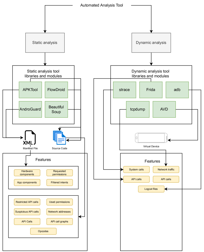
Figure 1 shows the architecture of the automated analysis tools.

Refer to caption — Figure 1: Automated analysis tool architecture

II-C Dynamic Analysis Tool

We developed a dynamic analysis tool that can run on the readily available Android emulators provided by Android SDK [17]. The virtual images in the emulators also allow root access which is essential for dynamic analysis. Here we describe the environment required to run the tool and the features extracted by the tool.

II-C1 Environment

We developed and tested the tool on Ubuntu, CentOS and Windows 10. The tool requires the following to run:

•

Python 3: All the dynamic modules require Python to run.
•

Frida-Android: The tool requires Frida’s Python library to hook to API calls during execution of an application.
•

Android Emulator: Our tool uses the emulator provided by Android SDK as the virtual environment to run the analysis. The emulator should be on the system path. We have tested the tool on Android 8, 9, 10 and 11 and we expect it to run on the upcoming Android 12.
•

The tool requires adb from Android SDK and it should be on the system path. The dynamic analysis tool connects to the virtual device using adb and executes commands on the emulator using adb.
•

Frida-server needs to be running on the virtual device to capture the hooked API calls while running the application.
•

The tool requires a static analysis report for an API calls analysis. If a static analysis report is not present, the dynamic tool requires APKTool to perform static analysis on the application.

II-C2 Feature Extraction

The dynamic analysis tool can extract the key dynamic features used in Android malware detection. These include system calls, API calls, logcat files and network traffic. The tool uses Android’s monkey tool to input virtual events that imitate an application’s user input. It allows the user to set the number of virtual events and/or the maximum time the application should run for.

We ran the application in a controlled environment, namely the Android emulator provided in the Android SDK. The tool has an option to hide the emulator to save memory but before running the analysis, the Android emulator needs to be set up.

Our dynamic analysis tool is comprised of the following modules:

System Calls:: The system calls module extracts and saves all the system calls made by the application during its run time using strace. Strace is a Linux utility used to monitor the interaction between the process (application) and the OS. While performing system calls analysis, it is essential to collect all the system calls that occur during run-time. From past works, we see researchers run the application and then retrieve the application process ID (pid) to monitor system calls associated with this. This approach might cause some system calls to be missed in the time between starting the application and running the strace tool. To mitigate against this, we run strace on the zygote process of the OS. The zygote process starts every other Android OS process. By monitoring the zygote process, we monitor all the processes in the OS. When the analysis ends, we filter out the system calls used by the application we are monitoring from the complete system call analysis extracted by monitoring the zygote process. The tool then saves the output in a separate file for every application.
Network Traffic:: Our tool uses Android emulator’s tcpdump to collect the complete network traffic of the application. It stores the resulting data in “pcap” files, later used to analyze and extract features. Wireshark [18] can process this file to analyze the application’s network traffic. It also saves a separate network traffic file for every application.
Android Logcat:: The tool uses logcat, a command line tool provided by Android SDK to dump all the messages and errors the device throws during the execution of the application. The adb utility runs logcat and saves the output in a file for further analysis.
API Calls:: The tool requires hooking of API calls beforehand to monitor execution of API calls during the run-time of an application. However, it is not computationally feasible to monitor the 130,000+ API calls present in the Android SDK. Therefore, the tool carries out the following steps: before starting the dynamic analysis, it checks if a corresponding static analysis report is present for the application. In addition to hooking the classic calls used in the literature of dynamic analysis tools [19], we also hooked application-specific API calls. If present, it hooks the API calls extracted in the static analysis report, or else, it performs a static analysis on the application using the static analysis tool. The dynamic analysis tool then hooks the API calls to monitor during the execution of the application using Frida. The tool saves a separate file with all the APIs called during execution for further analysis. As the process may involve static analysis, the API call module is optional in the dynamic analysis tool. By default, the tool monitors a pre-defined list of API calls; however to monitor the API calls mined from an application’s static analysis, the static analysis module is required.

II-D Evaluation Metrics

The following metrics are used to present results for the ML models trained in this study:

•

The confusion matrix. The results can be divided into four types as shown in Table I.

TABLE I: Confusion Matrix

Class Positive Negative

Malware TP FN

Benign FP FN
1. 1.
  
  True Positive (TP): The application is correctly predicted as malicious.
2. 2.
  
  False Positive (FP): The application is falsely predicted as malicious.
3. 3.
  
  True Negative (TN): The application is correctly predicted as benign.
4. 4.
  
  False Negative (FN): The application is falsely predicted as benign.
•

Accuracy: The percentage of correct predictions.

$Accuracy=\frac{TP+TN}{TP+TN+FP+FN}$ (1)
•

Precision: The percentage of correctly classified malware from all predictions of malware.

$Precision=\frac{TP}{TP+FP}$ (2)
•

True Positive Rate (TPR): The proportion of actual malware that are correctly identified. Also called recall.

$TPR=\frac{TP}{TP+FN}$ (3)

Class	Positive	Negative
Malware	TP	FN
Benign	FP	FN

•

F1-Score: The harmonic mean of precision and recall.

F_{1}=\frac{2*Precision*Recall}{Precision+Recall}=\frac{2*TP}{2*TP+FP+FN}

(4)

•

True Negative Rate (TNR): The proportion of actual benign applications that are correctly identified.

$TNR=\frac{TN}{FP+TN}$ (5)

In general, it is necessary to use a range of metrics in order to give a full picture of the performance of different ML models [20]. With this in mind, we report the accuracy, precision, F1-score, TPR and TNR for each model. TPR and TNR, in particular, help in understanding a model’s error rates. In the case of malware detection, it is particularly important to consider TPR, since a benign application labelled as malware is less likely to cause as many problems as malware labelled as benign.

The most common approach to comparing ML models in the Android malware literature is to report the average of metrics after using a resampling method like k-fold cross validation. Following this approach, we use standard 10-fold cross-validation (CV), and report the averages for all metrics. However, the average of a distribution can be misleading, particularly when there is a high variance between folds. To account for this, we report standard deviations and also carry out statistical tests when comparing averages of different approaches for malware detection. In a statistical test, a null hypothesis is set up (H₀): the average is equal for all sample population groups. A significant difference between the samples is found if the results from the test were to reject the null hypothesis and accept the alternative hypothesis (H_a): the average is not equal for all sample population groups.

In this work, we use the Kruskal–Wallis [21] omnibus test followed by pairwise Dunn’s [22] tests. Kruskal–Wallis is a non-parametric test used to determine if there are significant differences between the medians of two or more distributions. In this case, the distributions are the set of $k$ metric scores produced by each ML model across $k$ folds. If the test statistic p-value is less than a threshold level, the null hypothesis is rejected, indicating that there is a significant difference between the groups.

Kruskal-Wallis is an omnibus test and so does not indicate which sample group is statistically different from another. If Kruskal–Wallis finds a significant difference, Dunn’s test is then used to identify the samples that are statistically different from the others. If more than two models are being compared, a pairwise tournament between the ML models is used to determine the ML models with significant statistical differences. Dunn’s test automatically adjusts for multiple comparisons when used with Kruskal-Wallis. We use a threshold of p=0.05 for all statistical tests, i.e. a confidence of 95%.

II-E Core ML Models and Feature Selection Algorithms

Previous studies have used a diverse range of ML models. In general, we reimplement the model(s) used in the original study wherever possible. However, to provide better consistency and comparability across studies, we also augment the original studies with the following core set of ML models, if they are not already included: support vector machine (SVM), random forest (RF), decision tree (DT) and $k$ -nearest neighbour (kNN) [23]. All of these are widely used both within the Android malware detection literature (as surveyed in [9]) and the broader ML literature. We use grid search to tune the hyperparameters of all the models implemented. This is to ensure fairness when making comparisons between models.

Many studies also use feature selection algorithms to reduce feature counts to a manageable level. Again, whenever possible, we reimplement the approach(es) used in the original study. However, we also augment these with the following core set of feature selection algorithms: mutual information, chi-square, Pearson’s correlation coefficient (PCC), and variance threshold. All of these are widely used in the literature.

III Static Analysis

In this section, we focus on the use of static features in building Android malware detection models. Previous work in this area has considered various types of static features, including permissions, API calls, API call graphs and opcodes. We reimplement nine of these previous studies, focusing on those that were notable either in terms of the methodologies they used or the performance of their models on the original datasets. We also report the results of new experiments that are intended to fill in some of the knowledge gaps found in previous studies.

III-A Permissions and API calls

To begin with, we revisit one of the earliest studies that looked at permissions and API calls, carried out by Peiravian and Zhu in 2013 [24]. The authors compared models built using permissions alone, API calls alone, and a combination of both. In each case, they trained an SVM, a decision tree and a bagging classifier. They did not mention the kernel used for SVM, nor the base classifier used for bagging, so in our reimplementation we used the default choices of a linear kernel for SVM and decision trees as the base classifier. At the time of their study, the total number of permissions in Android was 130 and the total number of API calls was only 1,326. As shown in Table II, the numbers of both have grown since then, and by two orders of magnitude in the case of API calls.

TABLE II: Peiravian and Zhu dataset comparison

	Benign	Malware	Permissions	API Calls
Peiravian and Zhu	1,250	1,260	130	1,326
Our dataset	62,000	62,000	166	134,207

Table III reports the results both for Peiravian and Zhu’s original study and for our reimplementation using our much larger contemporary dataset. First of all, it is interesting to see that, despite the much larger feature and data set sizes, our results cover a similar range of accuracies. Peiravian and Zhu provided figures for accuracy, precision and recall in their evaluation. For completeness, we report the full set of metrics for our reimplementation.

Peiravian and Zhu found that models based only on API calls outperformed models based only on permissions. The figures in Table III show that this also appears to be the case for our reimplementation, with an even larger margin than in the original study.

We analysed the differences between models further by applying statistical tests. First, Kruskal-Wallis showed that there are significant differences in the accuracies reported in Table III (H = 50.04, p $<$ 0.05). Post hoc Dunn’s tests then showed that (i) the bagging and DT models using API calls perform better, on average, than all models that use permissions, and (ii) SVM models using API calls perform better, on average, than SVM models that use permissions. This supports the conclusion that API calls are more useful than permissions for building Android malware detection models.

All other group-wise differences were not significant at the 95% confidence level, suggesting that the exact choice of ML model is less important. However, we note that, for API calls, the bagging model had the best performance across all metrics, achieving an average accuracy of 96%.

TABLE III: Result comparison between Peiravian and Zhu. [24] and our reimplementation

Peiravian and Zhu. Results						Our Results
Dataset (Classifier)	Accuracy	Precision	F1-Score	TPR	TNR	Accuracy	Precision	F1-Score	TPR	TNR
Perm (SVM)	0.935	0.924	-	0.875	-	0.935 $\pm 0.002$	0.940 $\pm 0.002$	0.933 $\pm 0.002$	0.931 $\pm 0.002$	0.941 $\pm 0.001$
API (SVM)	0.958	0.917	-	0.957	-	0.953 $\pm 0.004$	0.957 $\pm 0.002$	0.954 $\pm 0.001$	0.956 $\pm 0.003$	0.958 $\pm 0.001$
Combined (SVM)	0.969	0.957	-	0.948	-	0.956 $\pm 0.002$	0.952 $\pm 0.002$	0.954 $\pm 0.002$	0.960 $\pm 0.001$	0.952 $\pm 0.001$
Perm (DT)	0.924	0.898	-	0.866	-	0.901 $\pm 0.003$	0.921 $\pm 0.003$	0.918 $\pm 0.002$	0.917 $\pm 0.004$	0.921 $\pm 0.001$
API (DT)	0.933	0.894	-	0.903	-	0.945 $\pm 0.002$	0.950 $\pm 0.002$	0.954 $\pm 0.001$	0.947 $\pm 0.002$	0.950 $\pm 0.002$
Combined (DT)	0.945	0.906	-	0.928	-	0.949 $\pm 0.002$	0.949 $\pm 0.003$	0.949 $\pm 0.001$	0.950 $\pm 0.001$	0.949 $\pm 0.002$
Perm (Bagging)	0.936	0.920	-	0.882	-	0.930 $\pm 0.002$	0.932 $\pm 0.001$	0.933 $\pm 0.003$	0.931 $\pm 0.001$	0.932 $\pm 0.002$
API (Bagging)	0.949	0.936	-	0.907	-	0.961 $\pm 0.002$	0.960 $\pm 0.003$	0.959 $\pm 0.002$	0.961 $\pm 0.002$	0.960 $\pm 0.002$
Combined (Bagging)	0.964	0.949	-	0.941	-	0.948 $\pm 0.001$	0.949 $\pm 0.002$	0.945 $\pm 0.002$	0.946 $\pm 0.001$	0.948 $\pm 0.002$

III-B A Closer Look at Permissions

Nevertheless, permissions are easier to extract than other static features. For this reason, they are widely used in practice. To provide more insight into the best way to use permissions for Android malware detection, we reimplemented a study by Wang et al. [25] that aimed to provide a more fine-grained view of the risk associated with permissions. Their study used two groups of Android permissions to build ML models: normal permissions, which are automatically granted by the system, and dangerous permissions, which provide access to private data or allow control over the device. For more information about these categories, see [26]. As shown in Table IV, the total number of normal and dangerous permissions is only slightly different in the current Android release.

Their study used four feature selection algorithms to identify the permissions that are most useful for building ML models: mutual information, PCC, sequential forward selection (SFS), and T-tests. They also used principal component analysis (PCA) as an alternative means of dimensionality reduction. In our reimplementation, we trained our four base ML models using feature sets derived both from the feature reduction methods used by Wang et al. and also our standard set of feature selection methods. We generated feature sets of sizes 10 to 70 features using each method.

TABLE IV: Wang et al. dataset comparison

	Benign	Malware	Permissions
Wang et al.	310,926	4,868	88
Our dataset	62,000	62,000	82

Table V shows the best results for each of Wang et al’s feature reduction methods, and for chi-square, which was our overall best performing feature selection method in terms of F1-score. The results from Wang et al. are for SVM models. For our results, we also indicate the best performing ML model for each feature reduction method. Our models performed significantly better than Wang et al’s in terms of F1-score. Although Wang et al. reported very high accuracies in their study, this is likely to be a reflection of their very imbalanced data set, and possibly an indication that their models overfit the majority class. This would also explain why their F1-scores were relatively low.

For our models, a positive Kruskal-Wallis test (H = 30.62, p $<$ 0.05) followed by pairwise Dunn’s tests showed that the only significant difference in mean accuracies was between the SVM trained on the SFS feature set and the other models. This does not allow us to draw any firm conclusions about which model or feature selection method is best.

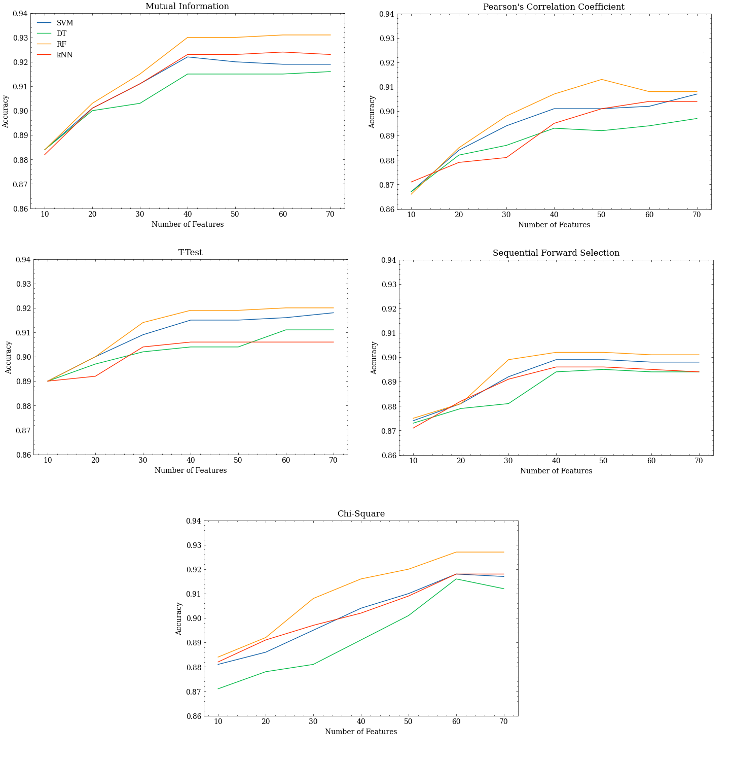
Fig. 2 shows how the accuracy of each model changes based on the size of the feature set. It can be seen that, for all models and feature selection methods, accuracy initially improves as the number of features is increased, but then reaches a plateau point. The best overall accuracy was achieved by RF and SVM models when using 40 permissions, and using more than 40 permissions did not lead to improvement in most cases. A notable difference from the findings of Wang et al. is that this plateau point comes later, which may indicate that more permissions are now required to build reliable malware detection models. Interestingly, the lists of the top 40 permissions produced by mutual information, PCC and T-test had 38 permissions in common across all the CV test folds. For chi-square, the best performing feature set, of 60 permissions, included all the permissions chosen by these other feature selection algorithms. Moreover, the models trained using chi-square permissions plateau later than the other feature selection models and so require more permissions to achieve high accuracy. The best chi-square model also achieved the highest F1-score.

TABLE V: Result comparison between Wang et al. [25] and our reimplementation. Accuracy and F1-scores for the original study are approximate values as they were read from plots provided by the authors.

Wang et al. Results						Our Results
Method	Accuracy	Precision	F1-Score	TPR	TNR	Method	Accuracy	Precision	F1-Score	TPR	TNR
Mutual information	0.996	-	0.895	0.923	-	Mutual information (RF)	0.930 $\pm 0.001$	0.932 $\pm 0.001$	0.929 $\pm 0.002$	0.931 $\pm 0.002$	0.931 $\pm 0.003$
PCC	0.996	-	0.895	0.923	-	PCC (RF)	0.907 $\pm 0.002$	0.910 $\pm 0.003$	0.905 $\pm 0.002$	0.902 $\pm 0.003$	0.911 $\pm 0.001$
T-Test	0.996	-	0.895	0.923	-	T-Test (RF)	0.919 $\pm 0.001$	0.920 $\pm 0.002$	0.921 $\pm 0.002$	0.919 $\pm 0.002$	0.921 $\pm 0.001$
SFS	0.996	-	0.895	0.923	-	SFS (SVM)	0.902 $\pm 0.002$	0.902 $\pm 0.003$	0.901 $\pm 0.002$	0.901 $\pm 0.001$	0.902 $\pm 0.002$
PCA	0.996	-	0.895	0.926	-	PCA (SVM)	0.928 $\pm 0.001$	0.926 $\pm 0.002$	0.927 $\pm 0.003$	0.932 $\pm 0.001$	0.925 $\pm 0.002$
Chi-square	-	-	-	-	-	Chi-square(RF)	0.927 $\pm 0.002$	0.923 $\pm 0.003$	0.946 $\pm 0.002$	0.901 $\pm 0.003$	0.949 $\pm 0.003$

Rathore et al. [27] further experimented with different feature selection and feature dimensionality reduction methods, with the aim of building an efficient model that used a minimal set of permissions. Apart from the original dataset with full permissions (OD), they used variance threshold (VT), PCA, and autoencoders (with one and three layers: AE-1L,AE-3L) to construct reduced feature sets. To this, we added our core set of feature selection algorithms. Unlike Wang et al., they carried out feature selection on the entire set of Android permissions, not just the normal and dangerous permissions. They trained six ML models for each of the feature selection/reduction methods: DT, kNN, SVM, RF, AdaBoost and DNNs (with two, four and seven layers). These were compared against models trained on the full set of 166 permissions.

TABLE VI: Result comparison between Rathore et al. [27] and our reimplementation

	Rathore et al. Results						Our Results
Classifier	Method	Accuracy	Precision	F1-Score	TPR	TNR	Method	Accuracy	Precision	F1-Score	TPR	TNR
Decision Trees	OD	0.926	-	-	0.919	-	OD	0.901 $\pm 0.003$	0.921 $\pm 0.003$	0.918 $\pm 0.002$	0.917 $\pm 0.004$	0.921 $\pm 0.001$
kNN	PCA	0.914	-	-	0.913	-	Mutual information	0.932 $\pm 0.002$	0.928 $\pm 0.001$	0.931 $\pm 0.002$	0.935 $\pm 0.001$	0.928 $\pm 0.002$
SVM	OD	0.910	-	-	0.894	-	AE-3L	0.933 $\pm 0.002$	0.927 $\pm 0.002$	0.935 $\pm 0.002$	0.942 $\pm 0.003$	0.927 $\pm 0.001$
Random Forest	OD	0.940	-	-	0.930	-	VT	0.949 $\pm 0.003$	0.948 $\pm 0.002$	0.950 $\pm 0.001$	0.951 $\pm 0.001$	0.949 $\pm 0.002$
AdaBoost	AE-1L	0.911	-	-	0.898	-	OD	0.928 $\pm 0.003$	0.922 $\pm 0.001$	0.927 $\pm 0.001$	0.934 $\pm 0.001$	0.921 $\pm 0.002$
DNN-2L	AE-1L	0.931	-	-	0.914	-	Mutual information	0.930 $\pm 0.002$	0.922 $\pm 0.003$	0.933 $\pm 0.002$	0.938 $\pm 0.003$	0.921 $\pm 0.001$
DNN-4L	VT	0.931	-	-	0.920	-	PCA	0.932 $\pm 0.001$	0.923 $\pm 0.002$	0.931 $\pm 0.001$	0.941 $\pm 0.003$	0.922 $\pm 0.002$
DNN-7L	OD	0.930	-	-	0.928	-	OD	0.927 $\pm 0.002$	0.922 $\pm 0.001$	0.925 $\pm 0.002$	0.933 $\pm 0.003$	0.921 $\pm 0.002$

Table VI summarises the performance metrics from our reimplementation, showing the figures for the most effective feature reduction method for each ML model. Our results are generally quite similar to those from the original study. Like Rathore et al., we found RFs to be the most effective model, with the highest mean values across all metrics. This is supported by a statistical analysis of the results in Table VI, where Dunn’s tests following a positive Kruskal-Wallis test (H = 54.58, p $<$ 0.05) indicated that RF accuracy was significantly higher than all other models except kNN. Our results also show that there is no particular value in reducing the set of permissions to those which are normal and dangerous prior to carrying out feature selection.

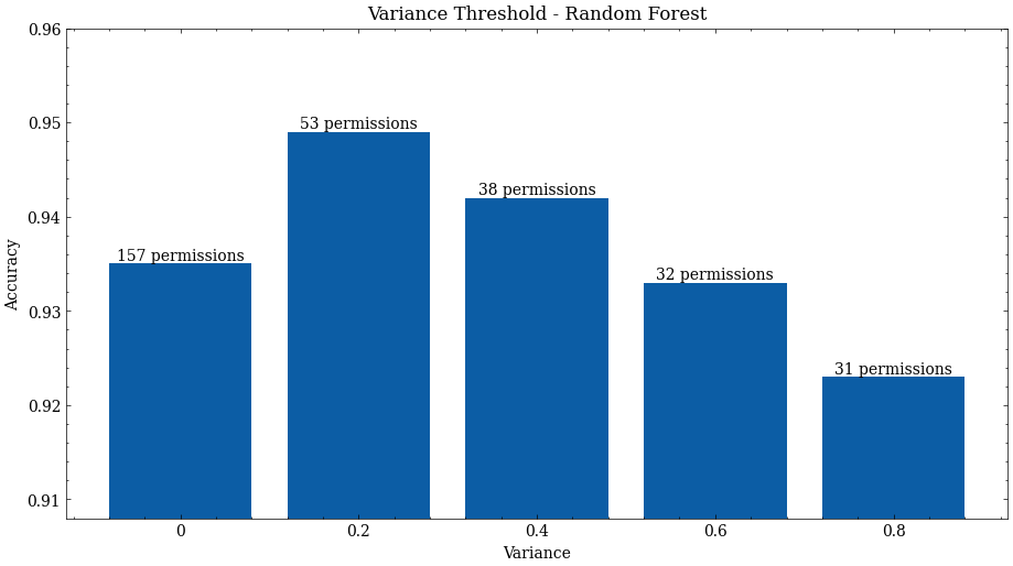
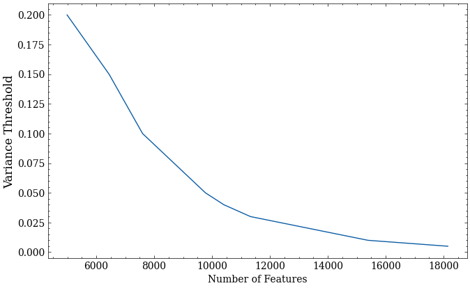
We found that RFs work best when combined with variance threshold. Digging down a bit further, Fig. 3 shows the effect of changing the threshold, indicating that lower thresholds work better. For a threshold of 0.2, the number of permissions can be reduced by 64%, whilst still producing better malware detection than when using all permissions.

To conclude, reasonable levels of performance can be achieved with permissions-based approaches, especially when the number of permissions is reduced using a feature selection algorithm, and RFs are used as the ML model. However, none of the permissions-based models we looked at were competitive against API call-based models.

III-C Representations of API Calls

Next, we take a closer look at the best way of building models based on API calls, beginning with a reimplementation of the research carried out by Ma et al. [28], who considered three different ways of representing feature usage within an application: API usage, API frequency and API sequences.

For API usage, each API call is represented by a binary feature indicating whether the call is used within an application. We created our version of this dataset by using the complete set of 134,207 API calls; i.e., each application is represented by a feature vector $A=\{API_{1},API_{2},API_{3},\dots API_{134207}\}$ , making this a high-dimensional feature set. This is the same dataset used for our earlier reimplementation of Peiravian et al. [24]. The API frequency data set is similar, except that each feature has an integer value, and indicates how many times each call is made within an application. For example, the feature vector for an application would be $M=\{5,4,0\}$ if $A=\{API_{1},API_{2},API_{3}\}$ and the application used $API_{1}$ 5 times, $API_{2}$ 4 times and $API_{3}$ 0 times.

For API sequences, each application is represented as a variable-length sequence of API calls. In our reimplementation, a call graph is extracted using the FLOWDROID module of our static analysis tool. The tool stores the APIs in chronological order and hence allows us to gather information on the order in which the application calls the APIs. We developed an algorithm which uses depth-first search (DFS) to obtain a set of routes for an application. The last API of every route is usually a system API call as user methods and user-defined APIs will always call system APIs. Therefore, we were able to extract system APIs that the application called in chronological order making an API sequence dataset. The resulting API system calls sequence is then converted into a numerical representation. For example, if we have a set of APIs $A=\{a,b,c,d\}$ then the applications are subsets of $A$ . If $M=[a,c,a,d]$ is a malware application and $B=[d,c,b,a]$ is a benign application, then the vector of $M$ will be $\{1,3,1,4\}$ and the vector of $B$ will be $\{4,3,2,4\}$ , where 1 represents $a$ , 2 represents $b$ , etc.

Ma et al. [28] used a different model for the three datasets: a DT for the API usage dataset, a deep neural network (DNN) for the API frequency dataset, and a long short-term memory (LSTM) model for the API sequence dataset. They also built an ensemble from the three models. In Table IX, we summarise our results from using this same approach. This indicates that the API frequency model performs the best, with both the usage and frequency models outperforming the API sequence models. We did not find any benefit to ensembling the models. This is in opposition to the findings of Ma et al. [28], for whom the best model was the ensemble, followed by the sequence model. Like Ma et al., we also looked more closely at the effect of network depth on the performance of the DNN and LSTM models. Table VII shows the results, showing that best performance is now achieved with a DNN of 16 layers, which is twice the depth of the best DNN found by Ma et al.

Kruskal-Wallis showed that the differences between the average accuracies in Table IX are significant (H = 35.63, p $<$ 0.05). Dunn’s tests indicated a significant difference between the frequency model and the sequence model, and no significant difference between the ensemble model, usage model and the frequency model. This supports the conclusion that the simpler usage and frequency-based models are more discriminative, at least within a contemporary Android environment.

A limitation of the original study was that different models were used for different representations, meaning that the effect of changing the representation could not be isolated from the effect of changing the model. To give more insight into whether the additional information embedded in the frequency representation over the usage representation is useful, we trained each of our core models, plus DNN, on both the API usage and frequency datasets. The results are shown in Tables XI and VIII respectively. Two things are notable: first, the differences in model accuracies are relatively small. Second, the ranking of the models changes depending on the representation, with DNNs doing best on the frequency dataset and RFs doing best on the usage dataset. Perhaps coincidentally, this justifies the model choices of Ma et al.

TABLE VII: Results from API Usage, API Frequency and API Sequence features

API Dataset	Layers	Accuracy	Precision	F1-Score	TPR	TNR
Usage	4 (DNN)	0.959 $\pm 0.002$	0.958 $\pm 0.002$	0.958 $\pm 0.002$	0.957 $\pm 0.003$	0.954 $\pm 0.002$
Usage	8 (DNN)	0.953 $\pm 0.002$	0.952 $\pm 0.003$	0.954 $\pm 0.002$	0.955 $\pm 0.003$	0.954 $\pm 0.002$
Usage	16 (DNN)	0.961 $\pm 0.001$	0.962 $\pm 0.003$	0.963 $\pm 0.002$	0.959 $\pm 0.001$	0.962 $\pm 0.001$
Usage	32 (DNN)	0.960 $\pm 0.001$	0.959 $\pm 0.002$	0.961 $\pm 0.002$	0.958 $\pm 0.003$	0.961 $\pm 0.001$
Frequency	4 (DNN)	0.961 $\pm 0.001$	0.955 $\pm 0.002$	0.958 $\pm 0.002$	0.963 $\pm 0.002$	0.956 $\pm 0.002$
Frequency	8 (DNN)	0.967 $\pm 0.002$	0.968 $\pm 0.003$	0.966 $\pm 0.002$	0.966 $\pm 0.002$	0.968 $\pm 0.002$
Frequency	16 (DNN)	0.970 $\pm 0.001$	0.971 $\pm 0.002$	0.969 $\pm 0.002$	0.969 $\pm 0.002$	0.971 $\pm 0.002$
Frequency	32 (DNN)	0.960 $\pm 0.002$	0.961 $\pm 0.002$	0.961 $\pm 0.002$	0.962 $\pm 0.002$	0.962 $\pm 0.002$
Sequence	4 (LSTM)	0.888 $\pm 0.002$	0.890 $\pm 0.002$	0.884 $\pm 0.002$	0.881 $\pm 0.001$	0.891 $\pm 0.003$
Sequence	8 (LSTM)	0.936 $\pm 0.003$	0.935 $\pm 0.004$	0.934 $\pm 0.001$	0.936 $\pm 0.002$	0.935 $\pm 0.001$
Sequence	16 (LSTM)	0.929 $\pm 0.001$	0.930 $\pm 0.002$	0.926 $\pm 0.002$	0.927 $\pm 0.002$	0.931 $\pm 0.002$
Sequence	32 (LSTM)	0.927 $\pm 0.002$	0.927 $\pm 0.001$	0.928 $\pm 0.002$	0.929 $\pm 0.002$	0.927 $\pm 0.002$

TABLE VIII: Evaluation metrics of the full API frequency feature set

Classifier	Accuracy	Precision	F1-Score	TPR	TNR
SVM	0.951 $\pm 0.001$	0.952 $\pm 0.002$	0.953 $\pm 0.002$	0.949 $\pm 0.002$	0.951 $\pm 0.002$
Random Forest	0.962 $\pm 0.001$	0.963 $\pm 0.002$	0.961 $\pm 0.002$	0.958 $\pm 0.001$	0.962 $\pm 0.003$
DT	0.942 $\pm 0.001$	0.943 $\pm 0.002$	0.941 $\pm 0.002$	0.944 $\pm 0.001$	0.945 $\pm 0.001$
kNN	0.943 $\pm 0.001$	0.944 $\pm 0.002$	0.945 $\pm 0.003$	0.948 $\pm 0.001$	0.949 $\pm 0.003$
DNN	0.970 $\pm 0.001$	0.971 $\pm 0.001$	0.969 $\pm 0.002$	0.979 $\pm 0.002$	0.971 $\pm 0.002$

TABLE IX: Result comparison between Ma et al. [28] and our reimplementation

Ma et al. Results							Our Results
Dataset	Model	Accuracy	Precision	F1-Score	TPR	TNR	Model	Accuracy	Precision	F1-Score	TPR	TNR
Usage	DT	-	0.968	0.965	0.962	-	Random Forest	0.966 $\pm 0.002$	0.968 $\pm 0.002$	0.966 $\pm 0.002$	0.964 $\pm 0.003$	0.969 $\pm 0.001$
Frequency	DNN(8)	-	0.977	0.974	0.971	-	DNN (16)	0.970 $\pm 0.001$	0.971 $\pm 0.001$	0.969 $\pm 0.002$	0.979 $\pm 0.002$	0.971 $\pm 0.002$
Sequence	LSTM(8)	-	0.985	0.986	0.988	-	LSTM (8)	0.935 $\pm 0.003$	0.935 $\pm 0.002$	0.936 $\pm 0.001$	0.936 $\pm 0.002$	0.935 $\pm 0.001$
Ensemble	Voting	-	0.991	0.99	0.988	-	Voting	0.965 $\pm 0.002$	0.963 $\pm 0.003$	0.962 $\pm 0.003$	0.967 $\pm 0.002$	0.963 $\pm 0.002$

III-D Reducing the Number of API Calls

Our results indicate that using API call features to build ML models leads to very good rates of malware detection. However, the large number of API calls available in the current Android SDK results in a high computational overhead when building models. In this section, we look at ways of reducing the size of the feature set.

Jung et al. [29] approached this by analysing the top 50 API calls used in benign applications then malware applications, resulting in two feature sets, one from each of the applications type, which they used to train RF models. The approach was evaluated using a dataset of 30,159 benign and 30,084 malicious applications. The results of our reimplementation are shown in Table X. Of the two feature sets, the use of the top 50 malware API calls leads to better models, and this is supported by a Kruskal-Wallis test, which showed a significant difference (H = 14.23, p $<$ 0.05). However, the rates of accuracy achieved in our experiments are considerably less than those reported by Jung et al, and the resulting models performed relatively poorly. This difference may in part be due to the much larger size of the API call set in contemporary versions of Android.

TABLE X: Result comparison between Jung et al. [29] and our reimplementation

Jung et al. Results						Our Results
Dataset	Accuracy	Precision	F1-Score	TPR	TNR	Accuracy	Precision	F1-Score	TPR	TNR
Top 50 Benign	0.999	-	-	-	-	0.701 $\pm 0.002$	0.677 $\pm 0.003$	0.721 $\pm 0.003$	0.632 $\pm 0.005$	0.771 $\pm 0.004$
Top 50 Malware	0.978	-	-	-	-	0.762 $\pm 0.002$	0.691 $\pm 0.002$	0.799 $\pm 0.001$	0.948 $\pm 0.002$	0.576 $\pm 0.002$

Although these results suggest that 50 API calls are insufficient to train accurate models, from a practical perspective, it remains desirable to work with smaller feature sets. Consequently, in Muzaffar et al. [30], we investigated the use of dimensionality reduction in API feature sets more broadly. We used a dataset of 20,000 benign applications and 20,000 malicious applications, and our results showed that the accuracy of the ML models could be improved by reducing the number of API calls by approximately 95% from the original set of 134,207. We trained SVM, RF, DT, AdaBoost and Naïve Bayes models, and used mutual information, variance threshold and PCC for feature selection.

TABLE XI: Result comparison between Muzaffar et al. [30] and our reimplementation

Muzaffar et al. Results						Our Results
Classifier	Accuracy	Precision	F1-Score	TPR	TNR	Accuracy	Precision	F1-Score	TPR	TNR
SVM	0.955 $\pm 0.002$	0.957 $\pm 0.004$	0.955 $\pm 0.002$	0.953 $\pm 0.004$	0.957 $\pm 0.004$	0.953 $\pm 0.004$	0.957 $\pm 0.002$	0.954 $\pm 0.001$	0.956 $\pm 0.003$	0.958 $\pm 0.001$
Random Forest	0.959 $\pm 0.001$	0.960 $\pm 0.001$	0.959 $\pm 0.002$	0.957 $\pm 0.001$	0.960 $\pm 0.002$	0.966 $\pm 0.002$	0.968 $\pm 0.002$	0.966 $\pm 0.002$	0.964 $\pm 0.003$	0.969 $\pm 0.001$
DT	0.940 $\pm 0.000$	0.938 $\pm 0.003$	0.941 $\pm 0.002$	0.943 $\pm 0.002$	0.938 $\pm 0.002$	0.945 $\pm 0.002$	0.950 $\pm 0.002$	0.954 $\pm 0.001$	0.947 $\pm 0.002$	0.950 $\pm 0.002$
Naïve Bayes	0.744 $\pm 0.002$	0.673 $\pm 0.003$	0.789 $\pm 0.002$	0.957 $\pm 0.002$	0.531 $\pm 0.005$	0.750 $\pm 0.001$	0.675 $\pm 0.001$	0.791 $\pm 0.002$	0.957 $\pm 0.002$	0.541 $\pm 0.003$
AdaBoost	0.943 $\pm 0.002$	0.943 $\pm 0.001$	0.943 $\pm 0.002$	0.944 $\pm 0.004$	0.942 $\pm 0.001$	0.943 $\pm 0.002$	0.943 $\pm 0.003$	0.943 $\pm 0.002$	0.944 $\pm 0.004$	0.943 $\pm 0.001$
kNN	-	-	-	-	-	0.942 $\pm 0.003$	0.942 $\pm 0.002$	0.944 $\pm 0.002$	0.941 $\pm 0.002$	0.944 $\pm 0.002$
DNN (16)	-	-	-	-	-	0.961 $\pm 0.001$	0.962 $\pm 0.003$	0.963 $\pm 0.002$	0.959 $\pm 0.001$	0.962 $\pm 0.001$

We reimplemented the study by using the current, considerably larger, dataset of 62,000 benign and 62,000 malicious applications. Table XI shows the results for the full API calls dataset. We also added kNN and Chi-square and compared the results. The RF models achieved the best results, followed by SVM. Naïve Bayes was included because of its training efficiency with large feature sets, but it performed poorly in terms of discrimination.

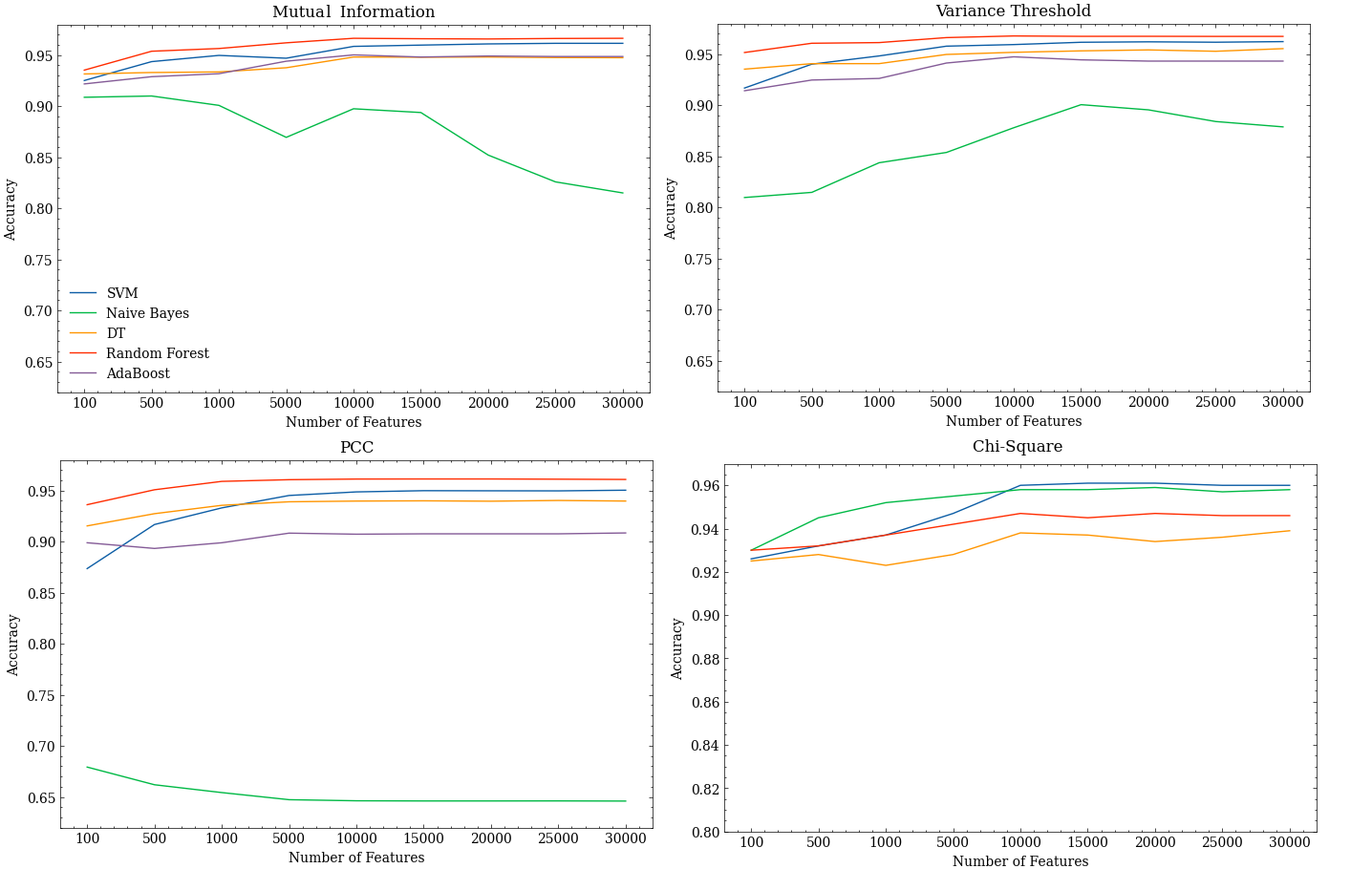
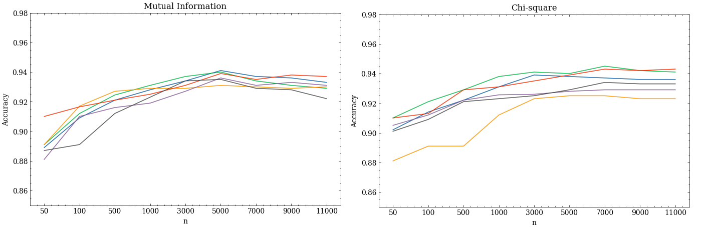
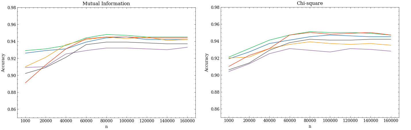
The feature selection algorithms were then used to reduce the feature set sizes to between 100 and 30,000 API calls. Fig. 4 shows the results for model accuracy, indicating that both the feature set size and the feature selection algorithm used have an impact on performance. In each case, it can be seen that accuracy plateaus beyond a certain number of API calls, supporting the idea that we only need to use a subset of the full Android API when training malware detection models.

Regardless of feature set size, RFs were the best models. Table XII shows the RF performance metrics for each of the feature selection algorithms. A Kruskal-Wallis test between the best performing RF model trained on the full API set and the models from Table XII indicated significant differences (H = 32.59, p $<$ 0.05). Post hoc Dunn’s tests then showed that feature sets derived using variance threshold led to significantly better models. Notably, these models could outperform the full API set models across all metrics while using only 5% (6,443) of the total API calls.

TABLE XII: Result comparison between Muzaffar et al’s best performing RF models using top features from feature selection algorithms and our reimplementation

Muzaffar et al. Results							Our Results
Feature Selection	Features	Accuracy	Precision	F1-Score	TPR	TNR	Features	Accuracy	Precision	F1-Score	TPR	TNR
Mutual information	10,000	0.962 $\pm 0.001$	0.960 $\pm 0.001$	0.961 $\pm 0.002$	0.959 $\pm 0.002$	0.963 $\pm 0.002$	10,000	0.967 $\pm 0.001$	0.969 $\pm 0.001$	0.967 $\pm 0.002$	0.963 $\pm 0.002$	0.970 $\pm 0.002$
Variance Threshold	6,443	0.961 $\pm 0.002$	0.964 $\pm 0.001$	0.961 $\pm 0.002$	0.958 $\pm 0.002$	0.964 $\pm 0.001$	6,443	0.968 $\pm 0.002$	0.971 $\pm 0.002$	0.968 $\pm 0.002$	0.965 $\pm 0.002$	0.971 $\pm 0.001$
PCC	15,000	0.951 $\pm 0.001$	0.952 $\pm 0.002$	0.951 $\pm 0.002$	0.938 $\pm 0.001$	0.965 $\pm 0.002$	15,000	0.961 $\pm 0.001$	0.970 $\pm 0.003$	0.961 $\pm 0.002$	0.950 $\pm 0.001$	0.971 $\pm 0.002$
Chi-Square	-	-	-	-	-	-	10,000	0.961 $\pm 0.003$	0.961 $\pm 0.004$	0.954 $\pm 0.002$	0.967 $\pm 0.001$	0.953 $\pm 0.001$

Fig. 5 shows variance values for feature set sizes of 100 to 30,000. This shows that about half the features have a variance below 0.025, which also signifies that many of the API calls are unlikely to play a useful role in discrimination. Overall, these results show that the number of API calls can be significantly reduced without loss of accuracy.

III-E The Drebin feature set

Arp et al’s Drebin dataset [16] is widely used in Android malware detection, both due to its availability and the large number of extracted features. They provided the following features for each application in the dataset:

•

Hardware components: The set of hardware components that an application requests.
•

Requested permissions: The set of permissions an application requests in their manifest file.
•

App components: The different components the application requests in the manifest.
•

Filtered intents: Intents used by the application; these could include intents like “BOOT_COMPLETED”. Applications use intents for inter-process communication.
•

Restricted API calls: Some critical calls are restricted by Android, these are looked for in the Dex files.
•

Used permissions: Felt et al. [31] introduced a method which was used to match API calls to permissions, hence obtaining the permissions which are actually used by the application.
•

Suspicious API calls: API calls that can access sensitive data.
•

Network addresses: These include IP addresses, URLs, and hostnames.

To get an indication of whether this feature set remains useful within a current Android environment, we extracted the same features from our set of contemporary applications. Table XIII outlines the differences in the datasets, showing a growth from 535,000 to three million distinct features. Table XIII also shows the accuracy of SVM models trained on these two datasets. This shows that, although not as effective as the API call models we looked at earlier, the Drebin feature set does remain competitive.

TABLE XIII: Framework comparison between Arp et al. [16] and our reimplementation

	Benign	Malware	No. of features	Accuracy
Drebin	123,453	5,560	535,000	0.94
Our Dataset	62,000	62,000	3 million reduced to 600,000	0.956

However, the size of the feature set means that it is computationally very challenging to train models. To address this, we only used the features that were used by at least two applications in the dataset, thereby reducing the feature set to 600,000. This allowed us to construct a dataset of a similar dimensionality to the original one. We then retrained the SVM models on this reduced dataset, and Table XIV shows that this led to a small reduction in accuracy.

We then looked at whether feature selection algorithms could be used to reduce the Drebin feature set to an even smaller set of useful features. Table XIV shows the results of applying the core set of feature selection algorithms and ML models. Although this significantly decreases the feature set size, it also leads to a significant decrease in accuracy. To conclude, the Drebin feature set does perform well; however, it may be difficult to use it in a production environment and reducing the number of features using feature selection algorithms decreases the performance of the models significantly.

TABLE XIV: Best results from Drebin feature set using feature selection algorithms

Feature Selection	Classifier	Number of Features	Accuracy	F1-Score	Precision	TPR	TNR
Feautres used twice	SVM	600,000	0.956 $\pm 0.002$	0.952 $\pm 0.003$	0.949 $\pm 0.002$	0.961 $\pm 0.002$	0.948 $\pm 0.001$
Mutual information	SVM	30000	0.897 $\pm 0.002$	0.895 $\pm 0.003$	0.887 $\pm 0.003$	0.897 $\pm 0.003$	0.891 $\pm 0.001$
Variance Threshold	SVM	35000	0.893 $\pm 0.002$	0.893 $\pm 0.002$	0.886 $\pm 0.004$	0.894 $\pm 0.002$	0.886 $\pm 0.002$
Chi-square	RF	25000	0.895 $\pm 0.002$	0.892 $\pm 0.004$	0.889 $\pm 0.003$	0.896 $\pm 0.002$	0.889 $\pm 0.002$
PCC	RF	35000	0.891 $\pm 0.002$	0.890 $\pm 0.002$	0.885 $\pm 0.002$	0.894 $\pm 0.002$	0.884 $\pm 0.003$

III-F Opcodes

Rather than a sequence of API calls, a program can instead be viewed, at a lower level, as a sequence of machine language instructions, or opcodes. A relatively small number of studies have considered opcode analysis as a basis for Android malware detection, and most have involved extracting features in the form of n-grams of opcodes, referred to as n-opcodes. For example, lets say that an application $A$ is the sequence $op_{1}$ , $op_{2}$ , $op_{3}$ , $op_{4}$ . A 2-gram, also known as bigram, representation of $A$ would be three bigrams, namely [ $op_{1}$ , $op_{2}$ ], [ $op_{2}$ , $op_{3}$ ] and [ $op_{3}$ , $op_{4}$ ]. To measure the benefits of this approach, and compare it against more traditional static features like permissions and API calls, we reimplement a study by Kang et al. [32], which considered both usage and frequency representations (see Section III-C) of n-opcodes.

Kang et al. used a dataset comprising 1,260 benign and 1,260 malware applications. They extracted n-opcodes of sizes one up to 10, and then used mutual information to reduce the number of features, before training NB, RF, SVM and partial decision tree (PART) models. In our reimplementation, we replaced PART with our standard DT model and also trained kNNs. We used our four core feature selectors. Table XV shows the number of n-opcodes for different values of $n$ up to 10 both for our dataset and the dataset used by Kang et al. This indicates a significant increase in the number of unique n-opcodes, particularly for larger values of $n$ , making feature selection a necessary step. Table XVI shows the number of features for each value of $n$ after carrying out feature selection using mutual information, which we found to be the most effective feature selector in our experiments.

TABLE XV: Number of unique n-opcodes for different values of

n

Kang et al.		Our Dataset
n	n-opcodes	n	n-opcodes
1	214	1	218
2	22,371	2	44,411
3	399,598	3	1,049,741
4	2,201,377	4	8,474,254
5	6,458,246	5	35,033,022
6	12,969,857	6	95,082,086
7	20,404,473	7	195,415,174
8	27,366,890	8	330,418,164
9	33,024,116	9	484,711,644

TABLE XVI: Number of selected n-opcodes using mutual information

n	Usage	Frequency
1	99	159
2	3,991	5,387
3	14,321	20,219
4	38,456	45,201
5	46,781	49,246
6	53,578	56,983
7	60,210	64,392
8	58,219	62,239
9	57,985	59,238
10	58,456	59,249

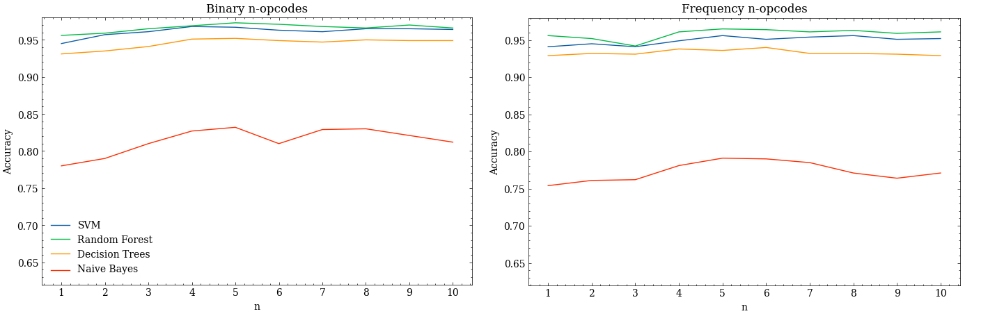
Fig. 6 shows the accuracy of the models trained on the features selected by mutual information, and also shows the effect of varying $n$ . In general, there appears to be little benefit to increasing $n$ much beyond 4, especially given the lower computational effort associated with smaller n-opcodes. Among the four ML models, it can be seen that RF models performed best for all values of $n$ and both feature representations. The average accuracies for models that use usage features were slightly higher than those which used frequency features, but the difference was small in comparison to the effect of ML model choice.

Table XVII summarises the performance of the best models. A Kruskal-Wallis test applied to these results indicates a significant difference (H = 36.44, p $<$ 0.05) between models, with Dunn’s tests showing that RF and SVM models are significantly better than the others. The performance of our models was broadly similar to those reported by Kang et al. Notably, these models have similar performance to models based on API calls. Opcodes take less time to extract compared to API calls and are much easier to train computationally on the base feature sets. However, it is much easier to interpret the API call results as APIs correspond to specific features in the Android SDK.

TABLE XVII: Result comparison between Kang et al. [32] and our reimplementation. F1-scores for the original study are approximate values as they were read from plots provided by the authors

Kang et al.							Our Results
Classifier	n	Accuracy	Precision	F1-Score	TPR	TNR	Classifier	n	Accuracy	Precision	F1-Score	TPR	TNR
Usage							Usage
SVM	3	-	-	0.98	-	-	SVM	4	0.968 $\pm 0.002$	0.971 $\pm 0.001$	0.971 $\pm 0.002$	0.961 $\pm 0.001$	0.971 $\pm 0.002$
Random Forest	4	-	-	0.98	-	-	Random Forest	5	0.973 $\pm 0.002$	0.979 $\pm 0.002$	0.975 $\pm 0.001$	0.965 $\pm 0.001$	0.979 $\pm 0.002$
Decision Trees	5	-	-	0.98	-	-	Decision Trees	5	0.952 $\pm 0.001$	0.952 $\pm 0.001$	0.951 $\pm 0.003$	0.949 $\pm 0.002$	0.952 $\pm 0.001$
Naïve Bayes	3	-	-	0.84	-	-	Naïve Bayes	5	0.832 $\pm 0.002$	0.834 $\pm 0.002$	0.828 $\pm 0.001$	0.821 $\pm 0.003$	0.838 $\pm 0.002$
Frequency							Frequency
SVM	4	-	-	0.96	-	-	SVM	5	0.956 $\pm 0.001$	0.954 $\pm 0.002$	0.956 $\pm 0.002$	0.958 $\pm 0.003$	0.954 $\pm 0.003$
Random Forest	8	-	-	0.97	-	-	Random Forest	5	0.965 $\pm 0.002$	0.969 $\pm 0.003$	0.967 $\pm 0.002$	0.961 $\pm 0.002$	0.970 $\pm 0.002$
Decision Trees	3	-	-	0.97	-	-	Decision Trees	6	0.940 $\pm 0.001$	0.942 $\pm 0.001$	0.937 $\pm 0.002$	0.935 $\pm 0.003$	0.941 $\pm 0.001$
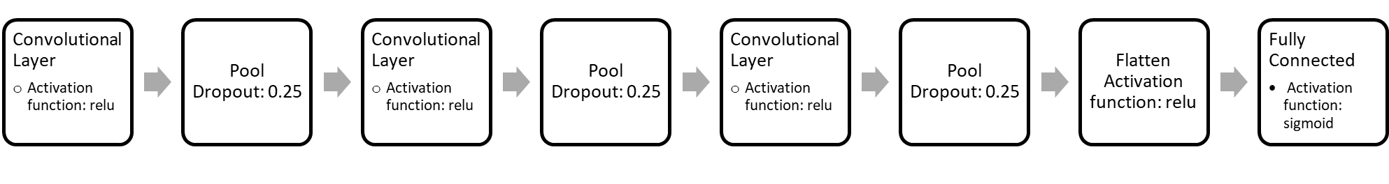
Naïve Bayes	4	-	-	0.85	-	-	Naïve Bayes	5	0.791 $\pm 0.002$	0.794 $\pm 0.001$	0.784 $\pm 0.003$	0.781 $\pm 0.002$	0.798 $\pm 0.001$

A common approach within deep learning is to convert numerical data into pseudoimages and use these to train a convolutional neural network (CNN). An example of this approach within the Android malware detection literature can be found in Xiao and Yang [33], who converted disassembled opcode files into RGB images. To determine whether this has any advantage over n-opcode encodings, we reimplemented the same approach and wrote an algorithm that converts opcode sequence files into RGB images. We then used these to train a CNN model, using the same CNN topology as Xiao and Yang, depicted in Fig. 7. Xiao and Yang trained and evaluated their model using a dataset of 4,406 benign and 6,134 malicious applications. Table XVIII compares evaluation metrics, and shows that there is generally no benefit to using this more complex modelling approach over the simpler models reported in Table XVII. This is supported by a statistical analysis, with Kruskal-Wallis (H = 56.44, p $<$ 0.05) and Dunn’s test showing Xiao and Yang’s approach to be significantly worse on our dataset than the best models in Table XVII.

TABLE XVIII: Result comparison between Xiao and Yang [33] and our reimplementation

Xiao and Yang’s Results					Our Results
Accuracy	Precision	F1-Score	TPR	TNR	Accuracy	Precision	F1-Score	TPR	TNR
0.93	0.936/0.921	0.94	0.944/0.910	0.903	0.913 $\pm 0.003$	0.912 $\pm 0.001$	0.916 $\pm 0.003$	0.921 $\pm 0.001$	0.911 $\pm 0.001$

III-G Comparison of static modelling approaches

To identify the best combination of features, ML models and feature selection algorithms for static analysis, we carried out a Kruskal-Wallis test followed by a pairwise comparison between the modelling approaches from this section. The results indicate that five of the models have statistically better accuracies than the others. Three of these are API call models: SVMs trained using 10,000 features selected using Chi-square, RF models trained using 10,000 features selected using mutual information, and RF models trained using 6,443 features selected using variance threshold Table (XII). The others are the RF usage 5-opcode model, trained using 46,781 features selected using mutual information Table (XVII) and DNN trained using API frequency Table (IX). Neither of these five modelling approaches appears to be significantly better than the others. This suggests that the best classes of features to use for static analysis are opcodes and API calls, and the best ML model to use is likely to be RF. However, the best choice of feature selection algorithm depends on the feature type and model type.

IV Dynamic Analysis

In this section, we focus on the use of dynamic features in building Android malware detection models. We reimplement five previous studies, and also report the results of new experiments that are intended to fill knowledge gaps found in these studies.

Dynamic analysis is not as common as static analysis. This is due to several factors, including the complex set up, relatively high computational costs, and the longer time required to run the analysis. A particular issue when running dynamic analysis is that each application needs to be executed on an emulator in order to record its dynamic features. During this process, some applications terminate unexpectedly. In some cases, the emulator itself crashes. Taking this into account, the set of applications for which we were able to complete dynamic analysis comprises 53,960 benign and 53,202 malware. However, this remains the largest and most up-to-date dataset used for dynamic analysis, to the best of our knowledge.

IV-A System Calls

System calls are the most commonly used dynamic features in the literature. Android applications use system calls to communicate with the kernel of the OS, and the strace module can be used to trace system calls that are made by an application during its runtime.

Ananya et al. [34] used sequences of system calls represented as unigrams, bigrams, and trigrams as the features of their models. They also used feature selection to select relevant features, and trained four ML models: linear regression, decision tree, RF and XGBoost. They used a dataset of 2,475 benign applications and 2,474 malware. The authors proposed two novel approaches to feature selection. The first, called SAILS, builds on the conventional feature selection algorithms mutual information, Chi-square and DFS. These are used to score the benign and malware features. SAILS then sorts the resulting scores in descending order, to create two sorted lists of benign and malware features. It then creates a final list that is the union of these two lists. The second feature selection algorithm proposed was WFS, which assigns weights to system calls. This is done by calculating the ratio of the number of occurrences of the system call in malware to the number of occurrences in the sum of benign and malware. In all the experiments, the authors used SAILS, WFS, mutual information, Chi-square and DFS to select relevant features. In our reimplementation, we also add PCC.

TABLE XIX: Result comparison between Ananya et al. [34] and our reimplementation

Ananya et al. Results

Our Results

Unigram

Classifier

Feature Selection

Accuracy

Precision

F1-Score

TPR

TNR

Feature Selection

Accuracy

Precision

F1-Score

TPR

TNR

SVM

Mutual information

0.928

\pm 0.001

0.926

\pm 0.001

0.924

\pm 0.003

0.922

\pm 0.002

0.929

\pm 0.001

Linear Regression

Mutual information

0.977

Mutual information

0.921

\pm 0.002

0.922

\pm 0.001

0.919

\pm 0.002

0.915

\pm 0.001

0.923

\pm 0.002

Random Forest

WFS

0.972

Mutual information

0.934

\pm 0.001

0.935

\pm 0.001

0.933

\pm 0.003

0.931

\pm 0.003

0.936

\pm 0.001

Decision Tree

Mutual information

0.965

Mutual information

0.925

\pm 0.002

0.926

\pm 0.002

0.921

\pm 0.002

0.922

\pm 0.001

0.926

\pm 0.001

XGBoost

WFS

0.966

Mutual information

0.933

\pm 0.001

0.931

\pm 0.001

0.930

\pm 0.002

0.931

\pm 0.002

0.932

\pm 0.001

kNN

Mutual information

0.922

\pm 0.002

0.918

\pm 0.002

0.921

\pm 0.002

0.917

\pm 0.003

0.923

\pm 0.002

Bigram

Classifier

Feature Selection

Accuracy

Precision

F1-Score

TPR

TNR

Feature Selection

Accuracy

Precision

F1-Score

TPR

TNR

SVM

Mutual information

0.941

\pm 0.002

0.939

\pm 0.002

0.942

\pm 0.003

0.938

\pm 0.002

0.943

\pm 0.001

Linear Regression

Chi-square

0.991

Mutual information

0.936

\pm 0.001

0.930

\pm 0.001

0.934

\pm 0.002

0.938

\pm 0.002

0.931

\pm 0.001

Random Forest

Chi-square

0.988

Chi-square

0.945

\pm 0.002

0.941

\pm 0.001

0.943

\pm 0.001

0.945

\pm 0.002

0.941

\pm 0.002

Decision Tree

Chi-square

0.977

Mutual information

0.931

\pm 0.003

0.929

\pm 0.001

0.929

\pm 0.001

0.931

\pm 0.002

0.929

\pm 0.003

XGBoost

DFS

0.994

Chi-square

0.943

\pm 0.002

0.943

\pm 0.001

0.942

\pm 0.003

0.939

\pm 0.002

0.944

\pm 0.002

kNN

Chi-square

0.932

\pm 0.001

0.929

\pm 0.003

0.931

\pm 0.001

0.926

\pm 0.002

0.931

\pm 0.002

Trigram

Classifier

Feature Selection

Accuracy

Precision

F1-Score

TPR

TNR

Feature Selection

Accuracy

Precision

F1-Score

TPR

TNR

SVM

Chi-square

0.947

\pm 0.001

0.945

\pm 0.002

0.946

\pm 0.002

0.947

\pm 0.002

0.951

\pm 0.003

Linear Regression

Mutual information

0.994

Mutual information

0.932

\pm 0.003

0.932

\pm 0.001

0.934

\pm 0.003

0.937

\pm 0.002

0.932

\pm 0.002

Random Forest

Mutual information

0.982

Chi-square

0.951

\pm 0.002

0.951

\pm 0.001

0.950

\pm 0.002

0.949

\pm 0.003

0.952

\pm 0.001

Decision Tree

WFS

0.987

Mutual information

0.945

\pm 0.003

0.943

\pm 0.001

0.942

\pm 0.002

0.943

\pm 0.002

0.943

\pm 0.001

XGBoost

Mutual information

0.992

Chi-square

0.950

\pm 0.002

0.948

\pm 0.001

0.947

\pm 0.002

0.947

\pm 0.002

0.948

\pm 0.002

kNN

Chi-square

0.942

\pm 0.002

0.941

\pm 0.001

0.943

\pm 0.002

0.938

\pm 0.001

0.941

\pm 0.002

Table XIX shows the best results for each ML model using unigrams, bigrams, and trigrams, and also indicates the most effective feature selection approach in each case. Notably, the performance metrics achieved in our reimplementation are substantially lower than those published in the original study. Ananya et al. reported accuracies of above 99%, whereas our best models achieved an accuracy of around 95%. This shows the importance of reimplementing studies using larger contemporary datasets, since it leads to the conclusion that dynamic analysis using system calls is less effective than the less expensive static analysis approaches considered earlier.

Neverthelesss, our results suggest that larger n-grams are more effective, and that RFs are again the best performing classifiers. A Kruskal-Wallis test between the models in Table XIX showed that there is a statistically significant difference in accuracy (H = 46.64, p $<$ 0.05). Post hoc Dunn’s tests confirmed that RFs outperformed the decision trees and linear regression models. Mutual information and Chi-square selected the best features for malware detection. Fig. 8 shows the accuracy rates of the ML models with different number of features selected by mutual information and Chi-square. The accuracy does not increase significantly, or in some cases dropped, after 90 features for unigrams, 5,000 features for bigrams using mutual information, 7,000 features for bigrams using Chi-square, and 80,000 features for trigrams.

TABLE XX: Result comparison between Malik et al. [35] and our reimplementation

Malik et al. Results						Our Results
Classifier	Accuracy	Precision	F1-Score	TPR	TNR	Classifier	Accuracy	Precision	F1-Score	TPR	TNR
kNN (3)	-	0.852	0.846	0.839	-	kNN (10)	0.820 $\pm 0.003$	0.869 $\pm 0.002$	0.806 $\pm 0.002$	0.752 $\pm 0.002$	0.887 $\pm 0.004$
LSTM (128)	-	0.786	0.859	0.946	-	LSTM (128)	0.7521 $\pm 0.001$	0.753 $\pm 0.003$	0.749 $\pm 0.002$	0.732 $\pm 0.002$	0.758 $\pm 0.001$

We reimplemented one more study that built models solely from system call features, carried out by Malik et al. [35]. This study is notable for using a different group of ML models and a different representation of the features. In particular, they used a 3-layer LSTM to classify malware based on the complete sequence of system calls used by an application, comparing this against a kNN model trained on a system call usage feature set. Both $k$ and the number of neurons per LSTM layer were optimised. Table XX shows the results. Like Malik et al., we found that there was no benefit to using a more complex, slower to train, sequence-based model, since the best kNN model (with $k=3$ ) substantially out-performed the best LSTM (with 128 neurons per layer). However, our LSTM model performed much better than the model reported by Malik et al.

To get a slightly broader perspective, we also trained our standard set of ML models using both the system call usage set and the corresponding system call frequency feature set. The results are shown in Table XXI. Reflecting our previous findings, the effect of moving between a usage-based and a frequency-based representation is relatively small — although, generally, the best models were found when using the usage-based feature set. Increasing the model set shows that kNN is not the best choice, with RF models leading to the best accuracy and F1-scores for both feature representations. This was confirmed by Kruskal-Wallis (H = 22.41, p $<$ 0.05) and Dunn’s tests, which showed RF to be statistically better than the other models, with no significant difference between RF usage and frequency models.

TABLE XXI: Evaluation metrics of usage and frequency system calls

Usage						Frequency
Classifier	Accuracy	Precision	F1-Score	TPR	TNR	Accuracy	Precision	F1-Score	TPR	TNR
SVM	0.830 $\pm 0.002$	0.843 $\pm 0.002$	0.827 $\pm 0.002$	0.811 $\pm 0.003$	0.849 $\pm 0.003$	0.821 $\pm 0.002$	0.823 $\pm 0.004$	0.824 $\pm 0.002$	0.810 $\pm 0.003$	0.832 $\pm 0.003$
Random Forest	0.845 $\pm 0.002$	0.858 $\pm 0.001$	0.842 $\pm 0.002$	0.826 $\pm 0.002$	0.863 $\pm 0.001$	0.839 $\pm 0.002$	0.835 $\pm 0.002$	0.833 $\pm 0.002$	0.856 $\pm 0.002$	0.821 $\pm 0.002$
DT	0.812 $\pm 0.003$	0.818 $\pm 0.002$	0.810 $\pm 0.002$	0.803 $\pm 0.002$	0.821 $\pm 0.001$	0.802 $\pm 0.002$	0.809 $\pm 0.003$	0.806 $\pm 0.003$	0.802 $\pm 0.001$	0.815 $\pm 0.003$
kNN	0.820 $\pm 0.003$	0.869 $\pm 0.002$	0.806 $\pm 0.002$	0.752 $\pm 0.002$	0.887 $\pm 0.004$	0.823 $\pm 0.002$	0.826 $\pm 0.003$	0.828 $\pm 0.003$	0.822 $\pm 0.001$	0.828 $\pm 0.001$

IV-B API Calls

Perhaps an obvious question at this point is whether API calls, which we found to be the most effective class of features in models resulting from static analysis, would also be beneficial for dynamic analysis. Afonso et al. [36] addressed this question to a certain extent by using information about both system calls and API calls in their models. Specifically, they used call frequencies as features, and a dataset of 2,968 benign and 4,552 malicious applications. We reimplemented their approach using SVM, RF, decision trees, kNN and Naïve Bayes. Afonso et al. also considered several other models, but those performed poorly in their study, so we did not reimplement them.

Table XXII shows the results of our reimplementation. The RF model does particularly well, and has comparable performance to the best static approaches. Notably, its performance is significantly higher than the system call-only models reported in the previous section (Kruksal-Wallis, H = 24.57, p $<$ 0.05, supported by Dunn’s tests). However, it should be noted those models used n-gram and sequence-based representations, rather than API call frequencies.

This still leaves the question of whether dynamic API calls alone can be used to build effective models. To address this, Table XXIII shows the performance of RF models trained solely on API call frequencies. The results are shown for both the full feature set and for feature sets reduced using the core feature selection algorithms. It can be seen that the performance of these models is a lot lower than the models that used both system and API calls. This seems to suggest that whilst the combination of dynamic system calls and dynamic API calls is more effective than either of these alone, information about dynamic API calls is not sufficient to train good models. This is an interesting finding, given that information about static API calls was sufficient to train good models. The poor performance of using the dynamic API calls alone could also be explained by the fact that while all system calls are monitored, only a subset of the API calls can be monitored due to their large number (134,207).

TABLE XXII: Result comparison between Afonso et al. [36] best RF model and our reimplementation

Afonso et al. Results						Our Results
Classifier	Accuracy	Precision	F1-Score	TPR	TNR	Classifier	Accuracy	Precision	F1-Score	TPR	TNR
Random Forest	0.968	0.975	0.968	0.961	0.976	Random Forest	0.962 $\pm 0.002$	0.968 $\pm 0.002$	0.964 $\pm 0.001$	0.959 $\pm 0.003$	0.969 $\pm 0.002$
						SVM	0.951 $\pm 0.001$	0.953 $\pm 0.001$	0.952 $\pm 0.001$	0.949 $\pm 0.002$	0.959 $\pm 0.002$
						kNN	0.946 $\pm 0.003$	0.943 $\pm 0.003$	0.946 $\pm 0.003$	0.943 $\pm 0.003$	0.948 $\pm 0.002$
						DT	0.936 $\pm 0.001$	0.938 $\pm 0.001$	0.935 $\pm 0.001$	0.933 $\pm 0.003$	0.938 $\pm 0.002$
						Naïve Bayes	0.857 $\pm 0.002$	0.860 $\pm 0.002$	0.856 $\pm 0.003$	0.851 $\pm 0.002$	0.862 $\pm 0.002$

We also show, in Table XXIII, the performance of models based upon usage (rather than frequency) of dynamic system and API calls. In common with our results from earlier studies, this shows that the choice of usage-based or frequency-based features has only a minor impact upon model performance. However, it is perhaps more notable within a dynamic context, where frequency-based features might be expected to contain information that were not available through static analysis alone, and highlights the fact that this additional information is not necessarily required in order to train good malware detection models.

TABLE XXIII: Evaluation metrics of usage and frequency dynamic API calls

Usage							Frequency
Feature Selection	Classifier	Accuracy	Precision	F1-Score	TPR	TNR	Classifier	Accuracy	Precision	F1-Score	TPR	TNR
Full Set	Random Forest	0.829 $\pm 0.002$	0.839 $\pm 0.003$	0.826 $\pm 0.003$	0.813 $\pm 0.003$	0.844 $\pm 0.001$	Random Forest	0.812 $\pm 0.002$	0.815 $\pm 0.001$	0.812 $\pm 0.002$	0.802 $\pm 0.002$	0.831 $\pm 0.001$
Mutual information	Random Forest	0.855 $\pm 0.003$	0.858 $\pm 0.002$	0.851 $\pm 0.003$	0.855 $\pm 0.001$	0.845 $\pm 0.001$	Random Forest	0.842 $\pm 0.003$	0.841 $\pm 0.001$	0.833 $\pm 0.003$	0.816 $\pm 0.003$	0.846 $\pm 0.003$
PCC	Random Forest	0.842 $\pm 0.002$	0.843 $\pm 0.002$	0.848 $\pm 0.002$	0.834 $\pm 0.002$	0.844 $\pm 0.003$	Random Forest	0.846 $\pm 0.002$	0.851 $\pm 0.002$	0.855 $\pm 0.003$	0.842 $\pm 0.002$	0.833 $\pm 0.001$
Variance Threshold	Random Forest	0.833 $\pm 0.002$	0.845 $\pm 0.002$	0.840 $\pm 0.002$	0.845 $\pm 0.003$	0.831 $\pm 0.002$	Random Forest	0.845 $\pm 0.001$	0.843 $\pm 0.001$	0.843 $\pm 0.003$	0.831 $\pm 0.003$	0.829 $\pm 0.001$
Chi-square	Random Forest	0.829 $\pm 0.002$	0.829 $\pm 0.002$	0.806 $\pm 0.002$	0.814 $\pm 0.002$	0.834 $\pm 0.001$	Random Forest	0.826 $\pm 0.003$	0.821 $\pm 0.002$	0.822 $\pm 0.002$	0.804 $\pm 0.002$	0.834 $\pm 0.002$

TABLE XXIV: Evaluation metrics of combination of usage system calls and API calls

Classifier	Accuracy	Precision	F1-Score	TPR	TNR
Random Forest	0.961 $\pm 0.002$	0.964 $\pm 0.002$	0.963 $\pm 0.001$	0.957 $\pm 0.003$	0.965 $\pm 0.002$
SVM	0.943 $\pm 0.001$	0.948 $\pm 0.001$	0.944 $\pm 0.001$	0.945 $\pm 0.002$	0.949 $\pm 0.002$
kNN	0.956 $\pm 0.003$	0.953 $\pm 0.003$	0.946 $\pm 0.003$	0.946 $\pm 0.003$	0.947 $\pm 0.002$
DT	0.933 $\pm 0.001$	0.938 $\pm 0.001$	0.936 $\pm 0.001$	0.931 $\pm 0.003$	0.935 $\pm 0.002$

IV-C Network Traffic

Dynamic analysis tools can also monitor network traffic during the execution of an application, and this provides another potentially useful source of information about the application’s behaviour. Previous works have focused on using network traffic features extracted from TCP and HTTP protocols.

Zulkifli et al. [37] used DT with TCP-based features in their study. They used a small dataset of 500 benign and 200 malicious applications, the latter assembled from two existing malware collections (Drebin and contagiodumpset). Notably, all the applications were executed on a real Android device. They extracted the following features:

•

The average packet size during the runtime of the dynamic analysis
•

The average of the number of packets sent per flow between host and client during the runtime of the dynamic analysis
•

The average of the number of packets sent per flow between client and host during the runtime of the dynamic analysis
•

The average packet size in terms of bytes sent per flow during the runtime of the dynamic analysis
•

The average packet size in terms of bytes received per flow during the runtime of the dynamic analysis
•

Ratio of the number of incoming bytes to outgoing bytes of every packet during the runtime of the dynamic analysis
•

The average number of packets received per second during the course of the dynamic analysis

TABLE XXV: Result comparison between Zulkifli et al. [37] and our reimplementation

Zulkifli et al. Results						Our Results
Dataset	Classifier	Accuracy	F1-Score	TPR	TNR	Classifier	Accuracy	Precision	F1-Score	TPR	TNR
drebin	DT	0.984	-	0.920	-	SVM	0.961 $\pm 0.001$	0.958 $\pm 0.002$	0.957 $\pm 0.002$	0.952 $\pm 0.002$	0.961 $\pm 0.002$
contagiodumpset	DT	0.976	-	0.920	-	Random Forest	0.977 $\pm 0.003$	0.969 $\pm 0.003$	0.981 $\pm 0.003$	0.978 $\pm 0.002$	0.971 $\pm 0.002$
						DT	0.973 $\pm 0.002$	0.967 $\pm 0.003$	0.977 $\pm 0.001$	0.973 $\pm 0.002$	0.969 $\pm 0.001$
						kNN	0.961 $\pm 0.001$	0.962 $\pm 0.003$	0.959 $\pm 0.002$	0.968 $\pm 0.001$	0.962 $\pm 0.001$

We extracted the same seven features for each of the applications in our dataset and trained the four core ML models. Table XXV shows the results, comparing our reimplementation with Zulkifli et al., who reported results separately for each of their two malware datasets. The best performing model was RF. Significantly, its accuracy and F1-score is the highest we have seen so far, suggesting that network traffic is an important source of information within a malware detection context.

Zulkifli et al. used a small dataset, presumably because they used a real Android device to perform their dynamic analysis. In this respect, it is interesting to see that our results show similar accuracy to the original paper. This supports the case for using an emulator to perform dynamic analysis, especially since an emulator is both a lot faster to configure and allows the OS image to be reloaded each time a dynamic analysis of an application is carried out, meaning that the analysis can be carried out in a controlled environment.

To further investigate network traffic features, we reimplemented another study by Wang et al. [38] involving network data. Wang et al. extracted both TCP and HTTP features from network traffic. Wang et al. used the same set of TCP features as Zulkifli et al., with the exception of average packet size. The features they extracted from HTTP headers were:

•

Host: This field specifies the host and port number that the request is sent to.
•

Request-URI: This is the uniform resource identifier from the requested source.
•

Request-Method: The action to be performed for a given resource. This includes GET and POST requests.
•

User-Agent: This holds information about the application, OS, vendor and version of the requesting user agent.

Wang et al. used a malware dataset consisting of 5,560 applications from the Drebin dataset and 8,312 benign applications downloaded from several application markets. The authors separately trained decision trees on both the HTTP and TCP datasets. In our reimplementation, we expanded on the original study by training our core set of ML models on the HTTP and TCP features both individually and in combination.

Table XXVI shows the results, and compares them against those from the original study. For our reimplementation, Table XXVI shows the results of the best ML models, which were RFs for both the HTTP and TCP feature sets. We observed no benefit to combining the two feature sets, but, for completeness, we also show results for the other models for both the HTTP and combined feature sets in Table XXVII. Whilst the results show good discrimination between benign applications and malware, we did not see the exceptionally high level of accuracy reported by Wang et al. for TCP features, and in fact found these to be less discriminative than HTTP features. These conclusions are supported by a positive Kruskal-Wallis test (H = 14.29, p $<$ 0.05) and Dunn’s tests.

TABLE XXVI: Result comparison between Wang et al. [38] and our reimplementation

Wang et al. Results								Our Results
Dataset	Classifier	Accuracy	Precision	F1-Score	TPR	TNR	Classifier	Accuracy	Precision	F1-Score	TPR	TNR
TCP	DT	0.982	-	-	-	-	Random Forest	0.973 $\pm 0.002$	0.967 $\pm 0.003$	0.977 $\pm 0.001$	0.973 $\pm 0.002$	0.969 $\pm 0.001$
HTTP	DT	0.997	-	-	-	-	Random Forest	0.963 $\pm 0.002$	0.961 $\pm 0.002$	0.965 $\pm 0.002$	0.965 $\pm 0.002$	0.961 $\pm 0.003$

TABLE XXVII: Evaluation metrics of the best performing network traffic models

Network Feature	Classifier	Accuracy	Precision	F1-Score	TPR	TNR
HTTP	SVM	0.941 $\pm 0.003$	0.942 $\pm 0.001$	0.941 $\pm 0.002$	0.943 $\pm 0.002$	0.946 $\pm 0.003$
HTTP	Random Forest	0.963 $\pm 0.002$	0.961 $\pm 0.002$	0.965 $\pm 0.002$	0.965 $\pm 0.002$	0.961 $\pm 0.003$
HTTP	DT	0.932 $\pm 0.002$	0.935 $\pm 0.003$	0.937 $\pm 0.004$	0.933 $\pm 0.001$	0.932 $\pm 0.002$
HTTP	kNN	0.951 $\pm 0.002$	0.956 $\pm 0.003$	0.955 $\pm 0.004$	0.949 $\pm 0.003$	0.959 $\pm 0.002$
TCP + HTTP	SVM	0.938 $\pm 0.002$	0.933 $\pm 0.003$	0.934 $\pm 0.004$	0.933 $\pm 0.001$	0.932 $\pm 0.003$
TCP + HTTP	Random Forest	0.952 $\pm 0.002$	0.953 $\pm 0.002$	0.956 $\pm 0.002$	0.955 $\pm 0.004$	0.951 $\pm 0.002$
TCP + HTTP	DT	0.929 $\pm 0.002$	0.926 $\pm 0.002$	0.925 $\pm 0.003$	0.922 $\pm 0.002$	0.925 $\pm 0.003$
TCP + HTTP	kNN	0.967 $\pm 0.004$	0.964 $\pm 0.002$	0.967 $\pm 0.001$	0.969 $\pm 0.002$	0.964 $\pm 0.003$

Although network traffic can be used to train accurate models, it is worth noting that consistently generating network traffic in an application is a major challenge. For instance, a network connection issue may result in the application not generating any network traffic. Furthermore, depending on the coverage of the dynamic analysis, i.e. the different activities invoked during the analysis, this may impact the network traffic captured.

IV-D Comparison of dynamic modelling approaches

To identify the best combination of ML models and feature selection algorithm on dynamic features, we carried out a Kruskal-Wallis test followed by a pairwise comparison between the models from section IV. This showed that the network traffic models from Table XXVII were significantly better than the others. However, as it can be a challenge to generate network traffic in dynamic analysis, it is useful to identify other well-performing dynamic approaches. Statistically, the best of the rest were the RF and XGBoost models trained on system call trigrams, selected using mutual information and Chi-square, respectively.

RF, as was the case for static features, was the best performing model for most of the dynamic features. Mutual information and Chi-square selected the most relevant features when used with both system calls and API calls. However, the results indicate that using static features generally produced the best results, with the notable exception of network traffic. System calls did lead to results comparable to the best performing static feature, API calls; however, the computational effort and time required to carry out a system call analysis probably outweighs the benefits.

V Hybrid Analysis

Hybrid analysis in theory uses the best of both worlds, static and dynamic features. As with dynamic analysis, hybrid studies are not as common as static analysis. In this section, we report and compare models that use hybrid features by reimplementing and extending past studies. As hybrid analysis uses dynamic features, in this section we use the slightly reduced dataset introduced in section IV, which consists of 53,960 benign and 53,202 malware.

We begin by reimplementing a study by Kandukuru and Sharma [39] that combined dynamic network traffic features with static permission features. The network traffic features included all seven of the TCP features listed in Section IV-C and the authors used a malware dataset of 1,200 applications collected from 2010 to 2011 to train a decision tree model. In our reimplementation, we trained all four core ML models. Table XXVIII compares their performance with Kandukuru and Sharma’s results. Since their performance is worse than models trained only on network features (see Tables tables XXV and XXVI), this suggests that there is no benefit to including information about static permissions.

TABLE XXVIII: Result comparison between Kandukuru and Sharma [39] and our reimplementation

Kandukuru and Sharma Results						Our Results
Classifier	Accuracy	Precision	F1-Score	TPR	TNR	Classifier	Accuracy	Precision	F1-Score	TPR	TNR
DT	0.956	-	-	0.95	0.96	Random Forest	0.943 $\pm 0.001$	0.941 $\pm 0.002$	0.945 $\pm 0.002$	0.948 $\pm 0.002$	0.940 $\pm 0.002$
						SVM	0.933 $\pm 0.002$	0.936 $\pm 0.001$	0.935 $\pm 0.002$	0.939 $\pm 0.001$	0.937 $\pm 0.003$
						DT	0.921 $\pm 0.003$	0.923 $\pm 0.003$	0.923 $\pm 0.002$	0.926 $\pm 0.003$	0.925 $\pm 0.001$
						kNN	0.936 $\pm 0.002$	0.938 $\pm 0.002$	0.939 $\pm 0.002$	0.941 $\pm 0.004$	0.937 $\pm 0.002$

To further investigate the use of hybrid features, we reimplemented a study based around two frequently used groups of static and dynamic features, permissions and system calls [40]. Kapratwar et al. carried out experiments using these features both separately and in combination. In the case of system calls, a frequency-based representation was used. For each experiment, the authors trained RF, decision trees, Naïve Bayes, logistic regression, kNN and SVM. However, as with most past hybrid works, Kapratwar et al. used a small dataset of just 103 malware and 97 benign applications. Therefore, a reimplementation of this approach using a larger contemporary dataset is essential to understand the effect of combining two of the most prevalent features in Android malware detection.

TABLE XXIX: Reimplementation of Kapratwar et al.’s [40] paper on the original feature set

Classifier	Accuracy	Precision	F1-Score	TPR	TNR
SVM	0.937 $\pm 0.01$	0.937 $\pm 0.02$	0.937 $\pm 0.02$	0.923 $\pm 0.01$	0.951 $\pm 0.02$
Random Forest	0.948 $\pm 0.02$	0.949 $\pm 0.01$	0.946 $\pm 0.01$	0.935 $\pm 0.01$	0.959 $\pm 0.02$
Naïve Bayes	0.860 $\pm 0.02$	0.861 $\pm 0.02$	0.860 $\pm 0.02$	0.831 $\pm 0.01$	0.889 $\pm 0.01$
Logistic Regression	0.937 $\pm 0.02$	0.938 $\pm 0.01$	0.936 $\pm 0.02$	0.925 $\pm 0.01$	0.949 $\pm 0.02$
kNN	0.921 $\pm 0.02$	0.924 $\pm 0.02$	0.922 $\pm 0.03$	0.886 $\pm 0.01$	0.958 $\pm 0.01$
Decision Trees	0.919 $\pm 0.02$	0.919 $\pm 0.02$	0.917 $\pm 0.01$	0.923 $\pm 0.02$	0.917 $\pm 0.02$

The results of our reimplementation are shown in Table XXIX, though note that we do not report the results of the original study in this case, since only AUC scores were provided. The performance of our models is comparable to the performance of models discussed earlier that used system calls or permissions separately, so again there does not appear to be any benefit to using a hybrid approach. We also used feature selection to select the most relevant features; mutual information was most useful for this, and Table XXX summarises the performance of the best models trained on the feature sets reduced according to mutual information. This suggests that there is a only a small benefit to doing this. However, as Fig. 9 shows, the number of features can be reduced by about a third without degrading performance. A Kruskal-Wallis test between the models in Table XXX showed that there was a statistically significant difference in accuracy (H = 25.62, p $<$ 0.05), and post hoc Dunn’s tests showed that the best performing ML model was RF.

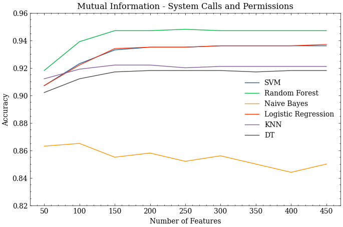
TABLE XXX: Reimplementation of Kapratwar et al.’s [40] paper on the best features selected by mutual information

Classifier	No. of Features	Accuracy	Precision	F1-Score	TPR	TNR
SVM	300	0.936 $\pm 0.02$	0.936 $\pm 0.01$	0.935 $\pm 0.02$	0.921 $\pm 0.01$	0.951 $\pm 0.02$
Random Forest	250	0.948 $\pm 0.02$	0.948 $\pm 0.03$	0.949 $\pm 0.03$	0.935 $\pm 0.01$	0.961 $\pm 0.02$
Naive Bayes	100	0.865 $\pm 0.03$	0.868 $\pm 0.02$	0.864 $\pm 0.01$	0.825 $\pm 0.01$	0.907 $\pm 0.02$
Logistic Regression	300	0.936 $\pm 0.02$	0.937 $\pm 0.02$	0.935 $\pm 0.02$	0.923 $\pm 0.02$	0.949 $\pm 0.02$
kNN	150	0.922 $\pm 0.02$	0.925 $\pm 0.01$	0.922 $\pm 0.01$	0.883 $\pm 0.03$	0.962 $\pm 0.01$
DT	200	0.918 $\pm 0.02$	0.917 $\pm 0.02$	0.916 $\pm 0.02$	0.920 $\pm 0.03$	0.915 $\pm 0.01$

VI Ensemble Models

In the hybrid approaches discussed in the previous section, a single ML model was built from a feature set containing more than one type of feature. However, a limitation of this approach is that all the features must be used with the same model, and must be represented in a way that is compatible with the same model. In this section, we explore a more flexible approach: ensemble modelling. Ensembles are ML models that combine the outputs of other, potentially diverse, ML models. A general benefit of ensembles is that they are often able to combine the strengths of their component models in order to provide a more robust overall prediction.

In the previous sections, we have reported the performance of various malware classification models. In this section, we explore whether better models can be created by combining these models. In particular, we construct voting ensembles from the best classification models seen so far. These base classifiers are listed in Table XXXI. Voting ensembles are constructed by selecting an odd number of models, and then outputting the majority decision, so they do not require further training. We considered each odd combination of base classifiers, and then sorted them by accuracy. Table XXXII lists the top five ensemble models according to this criterion.

TABLE XXXI: Classifiers used for ensemble models

ID	Feature Set	Type	Classifier	Feature Selection	Accuracy	F1-Score	Precision	TPR	TNR
$C_{1}$	API	Static	Random Forest	Mutual information	0.967 $\pm 0.001$	0.969 $\pm 0.001$	0.967 $\pm 0.002$	0.963 $\pm 0.002$	0.970 $\pm 0.002$
$C_{2}$	API	Static	Random Forest	Variance threshold	0.968 $\pm 0.002$	0.971 $\pm 0.002$	0.968 $\pm 0.002$	0.965 $\pm 0.002$	0.971 $\pm 0.001$
$C_{3}$	API	Static	Random Forest	Chi-square	0.961 $\pm 0.003$	0.915 $\pm 0.004$	0.954 $\pm 0.002$	0.967 $\pm 0.001$	0.953 $\pm 0.001$
$C_{4}$	Permissions	Static	Random Forest	Mutual information	0.930 $\pm 0.001$	0.932 $\pm 0.001$	0.929 $\pm 0.002$	0.931 $\pm 0.002$	0.931 $\pm 0.003$
$C_{5}$	Permissions	Static	Random Forest	Variance threshold	0.949 $\pm 0.003$	0.948 $\pm 0.002$	0.950 $\pm 0.001$	0.951 $\pm 0.001$	0.949 $\pm 0.002$
$C_{6}$	Opcodes (5-gram)	Static	Random Forest	Mutual information	0.973 $\pm 0.002$	0.979 $\pm 0.002$	0.975 $\pm 0.001$	0.965 $\pm 0.001$	0.979 $\pm 0.002$
$C_{7}$	System Calls (3-gram)	Dynamic	Random Forest	Chi-square	0.951 $\pm 0.002$	0.951 $\pm 0.001$	0.950 $\pm 0.002$	0.949 $\pm 0.003$	0.952 $\pm 0.001$
$C_{8}$	System Calls + API Calls (Usage)	Dynamic	Random Forest	None	0.961 $\pm 0.002$	0.964 $\pm 0.002$	0.963 $\pm 0.001$	0.957 $\pm 0.003$	0.965 $\pm 0.002$
$C_{9}$	Network Traffic (TCP)	Dynamic	Random Forest	None	0.977 $\pm 0.003$	0.969 $\pm 0.003$	0.981 $\pm 0.003$	0.978 $\pm 0.002$	0.971 $\pm 0.002$
$C_{10}$	Network Traffic (TCP + HTTP)	Dynamic	kNN	None	0.967 $\pm 0.004$	0.964 $\pm 0.002$	0.967 $\pm 0.001$	0.969 $\pm 0.002$	0.964 $\pm 0.003$
$C_{11}$	Network Traffic (TCP) + Permissions	Hybrid	Random Forest	None	0.943 $\pm 0.001$	0.941 $\pm 0.002$	0.945 $\pm 0.002$	0.948 $\pm 0.002$	0.940 $\pm 0.002$
$C_{12}$	Permissions + System Calls	Hybrid	Random Forest	Mutual information	0.948 $\pm 0.02$	0.948 $\pm 0.03$	0.949 $\pm 0.03$	0.935 $\pm 0.01$	0.961 $\pm 0.02$

TABLE XXXII: Ensemble model results

ID	Classifiers	Accuracy	F1-Score	Precision	TPR	TNR
$E_{1}$	$C_{1}$ + $C_{3}$ + $C_{7}$	0.978 $\pm 0.02$	0.976 $\pm 0.03$	0.975 $\pm 0.01$	0.979 $\pm 0.01$	0.977 $\pm 0.03$
$E_{2}$	$C_{2}$ + $C_{3}$ + $C_{7}$	0.971 $\pm 0.02$	0.971 $\pm 0.02$	0.970 $\pm 0.02$	0.971 $\pm 0.02$	0.967 $\pm 0.02$
$E_{3}$	$C_{1}$ + $C_{4}$ + $C_{6}$	0.959 $\pm 0.03$	0.955 $\pm 0.03$	0.953 $\pm 0.02$	0.956 $\pm 0.03$	0.952 $\pm 0.04$
$E_{4}$	$C_{3}$ + $C_{4}$ + $C_{9}$ + $C_{10}$ + $C_{12}$	0.969 $\pm 0.01$	0.970 $\pm 0.04$	0.965 $\pm 0.04$	0.966 $\pm 0.01$	0.969 $\pm 0.03$
$E_{5}$	$C_{4}$ + $C_{5}$ + $C_{8}$ + $C_{9}$ + $C_{10}$	0.954 $\pm 0.02$	0.953 $\pm 0.01$	0.952 $\pm 0.02$	0.955 $\pm 0.01$	0.958 $\pm 0.03$

Whilst all of these models perform better than the hybrid models presented in the previous section, Kruskal-Wallis and Dunn’s tests showed that none of them performed significantly better than the best standalone network traffic model. However, the $E_{1}$ ensemble does perform better than the best API call model, and, importantly, it achieves this by combining non-network features. This is significant because it avoids the challenges (discussed in Section IV-C) of recording network traffic during the dynamic analysis process, resulting in a model that may be more practical for real world deployment.

VII Discussion

This study allowed us to take a broader perspective on the Android malware-detection literature and, arguably for the first time, see how the different ML-based approaches to solving this problem work within contemporary Android systems. Some of the observations were surprising. For instance, our results suggest that there is generally little advantage to using dynamic analysis techniques, and that very accurate models can be built using relatively simple static features, particularly API call usage. The only scenario where dynamic analysis seemed to bring an advantage was when we built models based around network activity. However, this is expensive to implement in practice, since collection of network activity requires dynamic analysis at both training and inference time, and relies on features which are both difficult to collect and potentially brittle.

This is not the only instance where we observed a trade-off between the difficulty of extracting features, and the accuracy of the resulting models. Another notable example is the use of API calls versus permissions. Generating features based upon API calls requires the use of a static analysis tool. By comparison, permissions can be read directly from an application’s manifest file, a trivial operation. However, we found models trained on API call features to be significantly more accurate than models based upon permissions, showing that it is sometimes worth expending more effort on feature extraction.

We also found that hybrid models, built from a combination of static and dynamic features, were no better than those built from static or dynamic features alone. However, importantly, we showed that more accurate models can be constructed by ensembling the best static and dynamic models. Most significantly, we found that ensembling can be used to build models with accuracies comparable to the best network traffic models, but using less brittle features.

A recurring observation was the challenge caused by the growing complexity of Android. For instance, we observed that the number of API calls has grown by two orders of magnitude since early work on ML-based Android malware detection. This means the use of feature selection is now very important in order to reduce feature numbers down to manageable levels. Within this context, an important observation is that feature selection does not just reduce the computational resources needed for training; it also, in most cases, increases the accuracy of the resulting models. Most notably, we have shown that reducing the number of API calls by 95% leads to higher levels of malware discrimination. In general, we found mutual information and chi-square to be the most effective feature selectors.

The Drebin feature set has historically played an important role in ML-based malware detection studies. Although this feature set still performs reasonably well, our results suggest that it is no longer the best feature set to use, and is difficult to deploy due to the large number of features it entails when used within a contemporary Android environment. Unlike other feature sets we studied, it does not benefit from feature selection.

For features such as API calls, where it is possible to measure frequency of use in addition to whether they are used, this extra information generally does not improve a model’s ability to discriminate malware. This is a somewhat unexpected finding, but was observed consistently across a number of feature sets, both static and dynamic.

Beyond features, we also found that model choice is important, and random forests were surprisingly consistent in being the best performing models across the majority of experiments and feature sets. SVMs also performed well in general, but were more expensive to train than random forests. Naïve Bayes models generally performed poorly, suggesting that, for malware detection, interactions between features are important. A somewhat surprising observation, given their increasing prevalence within ML more generally, is that deep neural network models did not perform particularly well. However, there remains significant potential for applying newer deep learning models, such as transformers, to Android malware detection.

Finally, we observed that a number of the malware detection approaches reported in the literature performed significantly less well when we reimplemented and evaluated them on a large contemporary dataset. In many cases, this may be attributed to the increasing complexity of the Android environment; however, poor experimental practice is also likely to be a contributing factor, and we have observed many instances of authors falling into common ML pitfalls, including data leakage and the use of inappropriate metrics. Either way, it shows the importance of periodically reimplementing and reevaluating studies.

VIII Conclusions

In this work, we have have experimentally investigated the factors that affect model accuracy when applying machine learning to Android malware detection. We focused, in particular, on the importance of feature and model selection. An important component of our investigation was the reimplementation and reevaluation of existing approaches from the literature. This allowed us both to carry out a rigorous experimental comparison of these approaches, and to determine whether they remain relevant to contemporary Android systems. We also carried out a number of new experiments to fill in the knowledge gaps found in previous studies. These experiments were supported by the collection of a large up-to-date data set comprising 124,000 Android applications, equally divided between malware and benign applications. The tools used to create this dataset, as well as the tools we developed to extract features, are provided as a resource for the community.

A key observation is that features extracted using static analysis of Android APKs are often more effective than those extracted using dynamic analysis of running applications. This is important to know, since static analysis is much cheaper than dynamic analysis. Within this context, we found that simple representations of API usage led to very effective models, with accuracies of up to 96.8%. The exception to this is when features extracted from network traffic are used to build models. In our study, it is these models that provided the highest levels of malware discrimination, achieving accuracies of up to 97.7%. However, they are expensive to train and use, and rely on features that are difficult to collect and potentially brittle. Fortunately, we also showed that ensemble models built from non-network features can achieve a similar level of discrimination (97.8%), offering a more practical alternative for real world deployment.

Other notable observations include the importance of using feature selection algorithms when dealing with the complexity of modern Android systems, the high accuracy of random forest models in comparison to other ML models (including deep learners), and the relatively poor performance of the historically-important Drebin feature set. In future work, we plan to focus on online ML-based Android malware detection. Keeping a model up to date is important for accurate malware detection, and online learning can also be useful for drift detection. The sheer number of applications released everyday makes Android a prime candidate for online machine learning.

References

[1] S. O’Dea, “Forecast number of mobile users worldwide from 2020 to 2025,” [Online; Accessed: January 16, 2023]. [Online]. Available: https://www.statista.com/statistics/218984/number-of-global-mobile-users-since-2010/
[2] StatCounter, “Mobile operating system market share worldwide,” 2023, [Online; Accessed: January 16, 2023]. [Online]. Available: http://gs.statcounter.com/os-market-share/mobile/worldwide
[3] “Google play store,” https://play.google.com/store, [Online accessed January 10, 2023].
[4] G. Data, “G data mobile security report: Conflict in ukraine causes decline in malicious android apps,” Aug 2022.
[5] N. Elenkov, Android Security Internals. No Starch Press, 2015, vol. 2015, no. 6.
[6] I. M. Almomani and A. A. Khayer, “A comprehensive analysis of the android permissions system,” IEEE Access, vol. 8, pp. 216 671–216 688, 2020.
[7] Sufatrio, D. J. J. Tan, T.-W. Chua, and V. L. L. Thing, “Securing android: A survey, taxonomy, and challenges,” ACM Comput. Surv., vol. 47, no. 4, 5 2015. [Online]. Available: https://doi.org/10.1145/2733306
[8] M. Sikorski and A. Honig, Practical malware analysis: the hands-on guide to dissecting malicious software. no starch press, 2012.
[9] A. Muzaffar, H. R. Hassen, M. A. Lones, and H. Zantout, “An in-depth review of machine learning based android malware detection,” Computers & Security, p. 102833, 2022.
[10] “App downloads for android,” https://en.uptodown.com/android, [Online accessed July 31, 2021].
[11] “Apkmirror,” https://www.apkmirror.com/, [Online accessed July 31, 2021].
[12] “F-droid - free and open source android app repository,” https://www.f-droid.org/, [Online accessed July 31, 2021].
[13] “Virusshare,” https://virusshare.com, [Online accessed January 10, 2023].
[14] “Virustotal,” https://www.virustotal.com, [Online accessed January 10, 2023].
[15] R. Connor Tumbleson, “Apktool,” https://ibotpeaches.github.io/Apktool/, 2019.
[16] D. Arp, M. Spreitzenbarth, M. Hübner, H. Gascon, and K. Rieck, “Drebin: Effective and Explainable Detection of Android Malware in Your Pocket,” in Network and Distributed System Security Symposium (NDSS), no. August, 2014.
[17] Android Developers, “Download android studio & app tools android developers,” https://developer.android.com/studio, Jan 2023, [Online accessed January 10, 2023].
[18] “Wireshark,” https://www.wireshark.org/, [Online accessed January 10, 2023].
[19] “Mobile security framework (mobsf),” https://github.com/MobSF/Mobile-Security-Framework-MobSF.
[20] M. A. Lones, “How to avoid machine learning pitfalls: a guide for academic researchers,” 2021. [Online]. Available: https://arxiv.org/abs/2108.02497
[21] W. H. Kruskal and W. A. Wallis, “Use of ranks in one-criterion variance analysis,” Journal of the American statistical Association, vol. 47, no. 260, pp. 583–621, 1952.
[22] O. J. Dunn, “Multiple comparisons using rank sums,” Technometrics, vol. 6, pp. 241–252, 1964.
[23] T. Hastie, R. Tibshirani, and J. Friedman, The elements of statistical learning: data mining, inference, and prediction. Springer Science & Business Media, 2009.
[24] N. Peiravian and X. Zhu, “Machine Learning for Android Malware Detection Using Permission and API Calls,” in 2013 IEEE 25th International Conference on Tools with Artificial Intelligence. IEEE, nov 2013, pp. 300–305. [Online]. Available: http://ieeexplore.ieee.org/document/6735264/
[25] W. Wang, X. Wang, D. Feng, J. Liu, Z. Han, and X. Zhang, “Exploring permission-induced risk in android applications for malicious application detection,” IEEE Transactions on Information Forensics and Security, vol. 9, no. 11, pp. 1869–1882, 2014.
[26] Android Developers, “Permissions overview: Android developers,” https://developer.android.com/guide/topics/permissions/overview, October 2022, [Online accessed January 11, 2023].
[27] H. Rathore, S. K. Sahay, R. Rajvanshi, and M. Sewak, Identification of Significant Permissions for Efficient Android Malware Detection. Springer International Publishing, 2021, vol. 355. [Online]. Available: http://dx.doi.org/10.1007/978-3-030-68737-3_3
[28] Z. Ma, H. Ge, Y. Liu, M. Zhao, and J. Ma, “A Combination Method for Android Malware Detection Based on Control Flow Graphs and Machine Learning Algorithms,” IEEE Access, vol. 7, no. c, pp. 21 235–21 245, 2019.
[29] J. Jung, H. Kim, D. Shin, M. Lee, H. Lee, S. J. Cho, and K. Suh, “Android Malware Detection Based on Useful API Calls and Machine Learning,” Proceedings - 2018 1st IEEE International Conference on Artificial Intelligence and Knowledge Engineering, AIKE 2018, pp. 175–178, 2018.
[30] A. Muzaffar, H. Ragab Hassen, M. A. Lones, and H. Zantout, “Android malware detection using api calls: A comparison of feature selection and machine learning models,” in International Conference on Applied CyberSecurity. Springer, 2021, pp. 3–12.
[31] A. P. Felt, E. Chin, S. Hanna, D. Song, and D. Wagner, “Android Permissions Demystiﬁed,” in ACM Conference on Computer and Communications Security (CCS), 2011, pp. 627–637.
[32] B. J. Kang, S. Y. Yerima, K. McLaughlin, and S. Sezer, “N-opcode analysis for android malware classification and categorization,” 2016 International Conference on Cyber Security and Protection of Digital Services, Cyber Security 2016, pp. 13–14, 2016.
[33] X. Xiao and S. Yang, “An image-inspired and cnn-based android malware detection approach,” in 2019 34th IEEE/ACM International Conference on Automated Software Engineering (ASE). IEEE, 2019, pp. 1259–1261.
[34] A. Ananya, A. Aswathy, T. R. Amal, P. G. Swathy, P. Vinod, and S. Mohammad, “SysDroid: a dynamic ML-based android malware analyzer using system call traces,” Cluster Computing, vol. 6, 2020. [Online]. Available: https://doi.org/10.1007/s10586-019-03045-6
[35] Y. Malik, C. R. S. Campos, and F. Jaafar, “Detecting Android Security Vulnerabilities Using Machine Learning and System Calls Analysis,” Proceedings - Companion of the 19th IEEE International Conference on Software Quality, Reliability and Security, QRS-C 2019, pp. 109–113, 2019.
[36] V. M. Afonso, M. F. de Amorim, A. R. A. Grégio, G. B. Junquera, and P. L. de Geus, “Identifying Android malware using dynamically obtained features,” Journal of Computer Virology and Hacking Techniques, vol. 11, no. 1, pp. 9–17, 2015.
[37] A. Zulkifli, I. R. A. Hamid, W. M. Shah, and Z. Abdullah, “Android malware detection based on network traffic using decision tree algorithm,” Advances in Intelligent Systems and Computing, vol. 700, pp. 485–494, 2018.
[38] S. Wang, Z. Chen, L. Zhang, Q. Yan, B. Yang, L. Peng, and Z. Jia, “TrafficAV: An effective and explainable detection of mobile malware behavior using network traffic,” 2016 IEEE/ACM 24th International Symposium on Quality of Service, IWQoS 2016, 2016.
[39] S. Kandukuru and R. M. Sharma, “Android malicious application detection using permission vector and network traffic analysis,” in 2017 2nd International Conference for Convergence in Technology (I2CT), 2017, pp. 1126–1132.
[40] A. Kapratwar, F. Di Troia, and M. Stamp, “Static and dynamic analysis of android malware.” in ICISSP, 2017, pp. 653–662.