PAC-Bayesian Soft Actor-Critic Learning

Abstract

Actor-critic algorithms address the dual goals of reinforcement learning (RL), policy evaluation and improvement, via two separate function approximators. The practicality of this approach comes at the expense of training instability, caused mainly by the destructive effect of the approximation errors of the critic on the actor. We tackle this bottleneck by employing an existing Probably Approximately Correct (PAC) Bayesian bound for the first time as the critic training objective of the Soft Actor-Critic (SAC) algorithm. We further demonstrate that online learning performance improves significantly when a stochastic actor explores multiple futures by critic-guided random search. We observe our resulting algorithm to compare favorably to the state of the art on multiple classical control and locomotion tasks in terms of both sample efficiency and regret minimization.

1 Introduction

The process of searching for an optimal policy to govern a Markov Decision Process (MDP) involves solving two sub-problems: i) policy evaluation, and ii) policy improvement (Bertsekas and Tsitsiklis, 1996). The policy evaluation step concers with identifying a function that maps a state to its value, i.e. the total expected reward the agent will collect by following a predetermined policy. The policy improvement step updates the policy parameters such that the states with larger values are visited more frequently. Modern actor-critic methods (Peters et al., 2010; Schulman et al., 2015; Lillicrap et al., 2016; Schulman et al., 2017; Haarnoja et al., 2018) address the two-step nature of policy search by allocating a separate neural network for each step, a critic network for policy evaluation and an actor network for policy improvement. It is often straightforward to achieve policy improvement by taking gradient-ascent steps on actor parameters to maximize the critic output. However, as being the training objective of the actor network, the accuracy of the critic sets a severe bottleneck on the success of the eventual policy search algorithm at the target task. The state of the art attempts to overcome this bottleneck via using copies of critic networks or Bellman target estimators whose parameters are updated with time lag Lillicrap et al. (2016) and using the minimum of two critics for policy evaluation to tackle overestimation due to the Jensen gap (Fujimoto et al., 2018; Haarnoja et al., 2018).

The Probably Approximately Correct (PAC) Bayesian theory (Shawe-Taylor and Williamson, 1997; McAllester, 1999) develops analytical statements about the worst-case generalization performances of Gibbs predictors that hold with high probability (Alquier, 2021). The theory assumes the predictors to follow a posterior measure tunable to observations while maintaining similarity to a desired prior measure. In addition to being in widespread use for deriving analytical guarantees for model performance, PAC Bayesian bounds are useful for developing training objectives with learning-theoretic justifications in supervised learning (Dziugaite and Roy, 2017) and dynamical systems modeling (Haußmann et al., 2021). To date, the potential of using PAC Bayesian training objectives in the RL setups has remained relatively unexplored.

In this paper, we demonstrate how PAC Bayesian bounds can improve the performance of modern actor-critic algorithms when used for robust policy evaluation. We adapt an existing PAC Bayesian bound (Fard et al., 2012) developed earlier for transfer learning for the first time to train the critic network of a SAC algorithm (Haarnoja et al., 2018). We discover the following remarkable outcomes:

• A PAC Bayesian bound can predict the worst-case critic performance with high probability. Hence, when used as a training objective, it naturally overcomes the notorious value overestimation problem of approximate value iteration (Van Hasselt et al., 2016).

• The randomized critic expedites policy improvement when used as a guide for optimal action search via multiple shooting. It does so by sampling multiple one-step-ahead imaginary futures from the randomized critic and actor and chooses the action that gives the highest sampled state-action value.

Based on these two outcomes, we propose a novel algorithm called PAC Bayes for Soft Actor-Critic (PAC4SAC), which delivers consistent performance gains over not only the vanilla SAC algorithm but also alternative approaches to improve the robustness of online reinforcement learning algorithms. We observe our PAC4SAC to solve four continuous control tasks with varying levels of difficulty in fewer environment interactions and smaller cumulative regret than its counterparts. Figure 1 illustrates the idea.

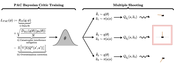
Figure 1: Our novel Probably Approximately Correct Bayes for Soft Actor Critic (PAC4SAC) algorithm trains a critic with random parameters $\theta$ for the first time using a PAC Bayesian bound as its training objective. The random critic also enables effective random optimal action search when used as a guide for a stochastic policy. The resulting algorithm solves online reinforcement learning tasks with fewer environment interactions and smaller cumulative regret than its counterparts.

2 Background

Online reinforcement learning.

We model a learning agent and its environment as a Markov Decision Process (MDP), expressed as a tuple $(\mathcal{S},\mathcal{A},p,p_{0},r,\gamma)$ comprising a $d_{s}-$dimensional continuous state space $\mathcal{S}:=\{s\in\mathbb{R}^{d_{s}}$ }, a $d_{a}-$dimensional continuous action space $\mathcal{A}:=\{a\in\mathbb{R}^{d_{a}}\}$, a reward function with bounded range $r:\mathcal{S}\times\mathcal{A}\rightarrow[r_{min},r_{max}]$, a reward discount factor $\gamma\in[0,1)$, a state transition distribution $p(s_{t+1}|s_{t},a_{t})$, and an initial state distribution $p_{0}(s_{0})$. We denote the visitation density function for state $s_{t+1}$ recursively as

$$p_{\pi}(s_{t+1})=\mathbb{E}_{p_{\pi}(s_{t})\pi(a_{t}|s_{t})}\left[p(s_{t+1}|s_{t},a_{t})\right],$$

where $\mathbb{E}_{p(x)}[f(x)]$ is the expectation of a function $f$ measurable by $p(x)$. The terminal condition of the recursion can be determined as $p_{\pi}(s_{0}):=p_{0}(s_{0})$. The goal of online reinforcement learning is to find a policy distribution $\pi(a_{t}|s_{t})$ such that both its entropy and the expected cumulative reward are maximized after a minimum number of environment interactions, in formal terms:

$$J(\pi) =\sum_{t=0}^{\infty}\mathbb{E}_{p_{\pi}(s_{t})\pi(a_{t}|s_{t})}\left[\gamma^{t}r(s_{t},a_{t})-\alpha\log\pi(a_{t}|s_{t})\right],$$

with respect to $\pi$ where the coefficient $\alpha>0$ is a parameter that regularizes the importance of the policy entropy on the training objective. We study the model-free case where the true state transition distribution $p(s_{t+1}|s_{t},a_{t})$ and the true reward function $r(s_{t},a_{t})$ are unknown to the agent and they are estimated during training from the observed state, action, reward, and next state tuples $(s_{t},a_{t},r_{t},s_{t+1})$.

Actor-critic learning.

Define the true value of a state-action pair under policy $\pi$, referred to as the actor, at time step $t$ of an interaction round with an environment as

$$Q_{\pi}(s_{t},a_{t}):=r(s_{t},a_{t})+\sum_{j=t}^{\infty}\mathbb{E}_{p_{\pi}(s_{j+1})\pi(a_{j+1}|s_{j+1})}\left[\gamma^{j-t}r(s_{j+1},a_{j+1})-\alpha\log\pi(a_{j+1}|s_{j+1})\right],$$

which satisfies the Bellman equation

$$Q_{\pi}(s_{t},a_{t})=r_{t}+\gamma\mathbb{E}_{p(s_{t+1}|s_{t},a_{t})\pi(a_{t+1}|s_{t+1})}[Q_{\pi}(s_{t+1},a_{t+1})]$$

using $r_{t}$ for the case when $r(s_{t},a_{t})$ is observed. As the true value function is unknown to us, we approximate it by a parametric function $Q_{\pi}^{\theta}(\cdot,\cdot)$ which is for instance a neural network, referred to as the critic. One incurs a Bellman error when $\exists(s_{t},a_{t})\in\mathcal{S}\times\mathcal{A}$ such that $Q_{\pi}^{\theta}(s_{t},a_{t})\neq Q_{\pi}(s_{t},a_{t})$, which can be quantified as

$$L(\theta;\mathcal{D})=\left(\mathbb{E}_{\pi(a_{t+1}|s_{t+1})}\left[r_{t}+\gamma Q_{\pi}^{\theta}(s_{t+1},a_{t+1})\right]-Q_{\pi}^{\theta}(s_{t},a_{t})\right)^{2}$$

for a sample set $\mathcal{D}=\{(s_{t},a_{t},r_{t},s_{t+1})|t=1,\ldots,N\}$ called a replay buffer. The Soft Actor-Critic (SAC) algorithm Haarnoja et al. (2018) is trained by alternating between policy evaluation $\arg\min_{\theta}L(\theta;\mathcal{D})$ which minimizes the Bellman error, and policy improvement

$$\arg\max_{\pi}\frac{1}{N}\sum_{t=1}^{N}\mathbb{E}_{\pi(a_{t}|s_{t})}[Q_{\pi}^{\theta}(s_{t},a_{t})-\log\pi(a_{t}|s_{t})]$$ (1)

which minimizes the Kullback-Leibler (KL) divergence between the policy distribution and a Gibbs distribution derived from the value predictor

$$\arg\min_{\pi}D_{KL}\left(\pi(a_{t}|s_{t})\Bigg{|}\Bigg{|}\frac{\exp(Q_{\pi}^{\theta}(a_{t}|s_{t}))}{\int\exp(Q_{\pi}^{\theta}(a^{\prime}_{t}|s_{t})da^{\prime}}\right),$$

where $D_{KL}(q(x)||p(x))=\mathbb{E}_{q(x)}\left[\log q(x)-\log p(x)\right]$ is the KL divergence for $q(x)$ and $p(x)$.

PAC Bayesian analysis.

Assume a prediction task from an input $x\in\mathcal{X}$ to output $y\in\mathcal{Y}$ with an unknown joint distribution $x,y\sim P$, the performance of which is quantified by a bounded loss functional $L(h(x),y):\mathcal{Y}\times\mathcal{Y}\rightarrow[0,L_{max}]$, where $h$ is a prediction hypothesis. A main concern of statistical learning theory is to find the tightest possible bound for the risk functional $R(h)$ that holds with highest possible probability based on its empirical estimate $R_{N}(h)$

$$R(h)=\mathbb{E}_{P(x,y)}[L(h(x),y)],~{}~{}~{}~{}R_{N}(h;\mathcal{D})=\frac{1}{N}\sum_{i=1}^{N}L(h(x_{i}),y_{i})$$

for an observation set $\mathcal{D}=\{(x_{i},y_{i})|i=1,\ldots,N\}$ consisting of $N$ independent and identically distributed (i.i.d.) observations taken from $P$. Bounds that satisfy these desiderata, referred to as Probably Approximately Correct (PAC) (Kearns and Vazirani, 1994), follow the structure below

$$Pr[R(h)\leq C(R_{N}(h;\mathcal{D}),\delta)]\geq 1-\delta$$ (2)

where $C(\delta)$ is an analytical expression dependent on the empirical estimate $R_{N}$ and a tolerance level $\delta\in(0,1)$. PAC Bayesian bounds (Shawe-Taylor and Williamson, 1997; McAllester, 1999) extend the PAC framework to the case where the hypothesis is assumed to be a Gibbs predictor that follows a distribution $h\sim q(h)$. The distribution $q(h)$ is called the posterior, which should desirably be similar to a prior distribution $p_{pri}(h)$ that represents domain knowledge or design choices to be imposed to the learning process. Differently from Bayesian inference, the relationship between the prior and the posterior distributions does not necessarily follow the Bayes theorem in the PAC Bayesian framework. It is sufficient that $p_{pri}$ is chosen a priori, while $q$ may be chosen after observing data. A PAC Bayesian bound has the structure

$$Pr\Bigg{[}\mathbb{E}_{q(h)}[R(h)]\leq C\Big{(}\mathbb{E}_{q(h)}[R_{N}(h;\mathcal{D})],\delta,D_{KL}(q(h)||p_{pri}(h))\Big{)}\Bigg{]}\geq 1-\delta.$$ (3)

The key difference of this bound from Eq. 2 is that it makes a statement about a distribution $q$ on the whole hypothesis space rather than a single hypothesis. Hence, it involves a complexity penalty at the scale of distributions $D_{KL}(q(h)||p_{pri}(h))$.

3 PAC Bayesian Soft Actor-Critic Learning

3.1 The problem and the hypothesis

Main problem.

The performance of online reinforcement learning algorithms is highly sensitive to the precision of the action-value function approximator, i.e. the critic, causing poor performance and sample inefficiency. This sensitivity is caused by two key factors:

• Overestimation bias: When the same function approximator is used for both prediction and target state estimation, the value of the target state is likely to be overestimated in Q-learning as a result of the approximation error. Even for additive noise term $\epsilon$ with zero mean, it holds that $\mathbb{E}_{\epsilon}[\max_{a}^{\prime}(Q_{\pi}^{\theta}(s^{\prime},a^{\prime})+\epsilon)]\geq\max_{a}^{\prime}Q_{\pi}(s^{\prime},a^{\prime})$ Thrun and Schwartz (1993). The same bias has been shown to exist also in actor-critic algorithms (Fujimoto et al., 2018) and to accumulate throughout the training period, resulting in a risk of significant drop in online learning performance.

• Catastrophic interference: Updating $\theta$ to reduce the Bellman error of a small group of states with poor value estimations affects also the other states, many of which may already have accurate value estimations (Pritzel et al., 2017).

The commonplace solutions to mitigate these problems are two-fold:

• Twin critics: Learning two critics concurrently $Q_{\pi}^{\theta_{1}}$ and $Q_{\pi}^{\theta_{2}}$ and using $\min(Q_{\pi}^{\theta_{1}}(s,a),Q_{\pi}^{\theta_{2}}(s,a))$ for all state-action pair evaluations.

• Polyak averaging: Using copies of critics $Q_{\pi}^{\theta^{\prime}}$ for target evaluation when calculating Bellman errors, whose parameters are updated with time lag $\theta^{\prime}:=\tau\theta+(1-\tau)\theta^{\prime}$ where $\tau\in(0,1)$.

We aim to improve the SAC algorithm Haarnoja et al. (2018) by modifications guided by the following hypothesis.

Main hypothesis.

We claim that training a randomized critic with a PAC-Bayesian generalization performance bound reduces the sensitivity of the SAC algorithm to factors (a) and (b). We further claim that using all sources of randomization in the model for optimal action search brings additional performance boost.

3.2 PAC-Bayesian soft policy evaluation

We define our loss as the Bellman error

$$L(Q_{\pi}^{\theta}(s_{t},a_{t}),y_{t}) =\mathbb{E}_{p(s_{t+1}|s_{t},a_{t})\pi(a_{t+1}|s^{\prime}_{t})}\left[(y_{t}-Q_{\pi}^{\theta}(s_{t},a_{t}))^{2}\right]$$ (4)

for an arbitrary time step $t$ where

$$y_{t}=r_{t}+\gamma Q_{\pi}^{\theta}(s_{t+1},\widetilde{a}_{t+1})-\log\pi(\widetilde{a}_{t+1}|s_{t+1})$$

is the soft Bellman target with $\widetilde{a}_{t+1}\sim\pi(a_{t+1}|s_{t+1})$. Then the risk functional and its empirical estimate follow as

$$R(\theta;\pi) =\mathbb{E}_{p_{\pi}(s_{t})\pi(a_{t}|s_{t})}\left[(Q_{\pi}^{\theta}(s_{t},a_{t})-y_{t})^{2}\right],~{}~{}R_{N}(\theta;\pi,\mathcal{D})=\frac{1}{N}\sum_{t=1}^{N}\left(Q_{\pi}^{\theta}(s_{t},a_{t})-y_{t}\right)^{2}$$

for a replay buffer $\mathcal{D}=\{(s_{t},a_{t},r_{t},s_{t+1})|t=1,\ldots,N\}$ comprising a non-i.i.d. set of observations from the target environment and a parameterized hypothesis space $\mathcal{H}_{\pi}:=\{Q_{\pi}^{\theta}|\theta\in\Theta\}$. Let us introduce the soft Bellman backup operator with respect to a stochastic policy $\pi$ as

$$T_{\pi} Q_{\pi}^{\theta}(s_{t},a_{t})=r(s_{t},a_{t})+\mathbb{E}_{p(s_{t+1}|s_{t},a_{t})\pi(a_{t+1}|s_{t+1})}\left[\gamma Q_{\pi}^{\theta}(s^{\prime}_{t},a^{\prime}_{t})-\log\pi(a_{t+1}|s_{t+1})\right].$$

Then provably we have

$$\forall(s_{t},a_{t}),~{}~{}(T_{\pi}Q_{\pi}^{\theta}(s_{t},a_{t})- Q_{\pi}^{\theta}(s_{t},a_{t}))^{2}=0\iff Q_{\pi}^{\theta}=Q_{\pi}$$

which holds only under no approximation error and no estimation error, that is a hypothesis space that contains $Q_{\pi}$, a consistent learning algorithm, and infinite amount of data. Hence it is crucial for a reinforcement learning algorithm to robustly handle a level of approximation error. Our goal is to upper bound this error with high probability. Defining the squared weighted $L_{2}$ norm as $\lVert A(s)\rVert_{\rho(s)}^{2}=\int(A(s))^{2}\,\mathrm{d}\rho(s)$ for a function $A(\cdot)$ measurable by $p$, we get

$$||Q_{\pi}^{\theta}(s_{t},a_{t})- Q_{\pi}(s_{t},a_{t})||_{p_{\pi}(s_{t})\pi(a_{t}|s_{t})}^{2}\leq\frac{1}{(1-\gamma)^{2}}\Big{|}\Big{|}\mathbb{E}_{\pi(a_{t}|s_{t})}[T_{\pi}Q_{\pi}^{\theta}(s_{t},a_{t})-Q_{\pi}^{\theta}(s_{t},a_{t})]\Big{|}\Big{|}_{p_{\pi}(s_{t})}^{2}$$

which characterizes an upper bound on the value approximation error in terms of the Bellman error. See Lemma A.3.1 in Appendix for the proof. We can construct a PAC-Bayesian bound by relating this inequality to the risk functional via the identity below:

$$\lVert T_{\pi}Q_{\pi}^{\theta}(s_{t},a_{t})-Q_{\pi}^{\theta}(s_{t},a_{t})\rVert_{p_{\pi}(s_{t})\pi(a_{t}|s_{t})}^{2}=\mathbb{E}_{p_{\pi}(s_{t})\pi(a_{t}|s_{t})}\left[\left(T_{\pi}Q_{\pi}^{\theta}(s_{t},a_{t})-Q_{\pi}^{\theta}(s_{t},a_{t})\right)^{2}\right]$$

$$=\mathbb{E}_{p_{\pi}(s_{t})\pi(a_{t}|s_{t})}\Bigg{[}\Bigg{(}Q_{\pi}^{\theta}(s_{t},a_{t})-r(s_{t},a_{t})$$ (5)

$$\qquad\qquad\qquad-\mathbb{E}_{p(s_{t+1}|s_{t},a_{t})\pi(a_{t+1}|s_{t+1})}\Big{[}\gamma Q_{\pi}^{\theta}(s_{t+1},a_{t+1})-\log\pi(a_{t+1}|s_{t+1})\Big{]}\Bigg{)}^{2}\Bigg{]}$$

$$=R(\theta;\pi)-\mathbb{E}_{p_{\pi}(s_{t})\pi(a_{t}|s_{t})}\Bigg{[}r(s_{t},a_{t})+\gamma\mathbb{V}_{p(s_{t+1}|s_{t},a_{t})}\Big{[}\mathbb{E}_{\pi(a_{t+1}|s_{t+1})}[Q_{\pi}^{\theta}(s_{t+1},a_{t+1})]\Big{]}\Bigg{]},$$

where $\mathbb{V}_{p(x)}[f(x)]$ denotes the variance of $f(x)$ dependent on a random variable $x$ distributed as measure $p(x)$. This construction allows us to straightforwardly adapt the PAC Bayesian bound of Fard et al. (2012), resulting in the theorem below.

Theorem 3.1.

Let $c_{1},c_{2}\in\mathbb{Z}^{+}$ be arbitrary constants, $p_{pri}$ and $q$ be prior and posterior measures respectively defined on $\Theta$, a set of observations $\mathcal{D}=\{(s_{t},a_{t},r_{t},s_{t+1})|t=1,\ldots,N\}$ following a Markov Decision Process $(\mathcal{S},\mathcal{A},p,p_{0},r,\gamma)$, then for any $N\in\mathbb{N}^{+}$ and $0<\delta<1$ it holds with probability greater than $1-\delta$ that:

$$||Q_{\pi}^{\theta}(s_{t},a_{t}) -Q_{\pi}(s_{t},a_{t})||_{p_{\pi}(s_{t})\pi(a_{t}|s_{t})q(\theta)}^{2}\leq$$

$$\frac{1}{(1-\gamma)^{2}}\Bigg{(}\mathbb{E}_{q(\theta)}[R_{N}(\theta;\pi,\mathcal{D})]+\sqrt{\frac{\log\left(\frac{c_{2}N}{c_{1}(r_{max}+|r_{min}|)^{2}\delta}\right)+D_{KL}(q(\theta)||p_{pri}(\theta))}{\frac{N}{(r_{max}+|r_{min}|)^{2}c_{1}}-1}}$$

$$\qquad-\mathbb{E}_{q(\theta)p_{\pi}(s_{t})\pi(a_{t}|s_{t})}\Bigg{[}r(s_{t},a_{t})+\gamma\mathbb{V}_{p(s_{t+1}|s_{t},a_{t})}\Big{[}\mathbb{E}_{\pi(a_{t+1}|s_{t+1})}[Q_{\pi}^{\theta}(s_{t+1},a_{t+1})]\Big{]}\Bigg{]}\Bigg{)}.$$

3.3 The PAC4SAC algorithm

Assume a parametric family of measures defined on $\Theta$, i.e. $\{q(\theta;\phi)|\phi\in\Phi\}$ for some parameter space $\Phi$. For instance if $q$ is chosen to be normal distributed, then $\Phi$ is the set of all possible mean and variance values. The choice of coefficients $c_{1},c_{2}$ would affect the outcome when the goal is to provide quantitative performance guarantees. As our concern is to develop a training objective for the critic, we simplify the bound while keeping it monotonic with respect to its original form. Choosing $c_{1}=N/(r_{max}+|r_{min}|)^{2})$ and $c_{2}=1$, dropping the terms that are constant with respect to $\phi$, and neglecting the effect of $\log(\delta)$ in the numerator we attain the critic training loss below:

$$L_{PAC4SAC}(\phi):= \underbrace{\mathbb{E}_{q(\theta;\phi)}[R_{N}(\theta;\pi,\mathcal{D})]}_{i)~{}\mathrm{Data~{}fit}}+\underbrace{\sqrt{\frac{D_{KL}(q(\theta;\phi)||p_{pri}(\theta))}{N}}}_{\begin{subarray}{c}\mathrm{ii)~{}Catastrophic~{}interference}\\ \mathrm{mitigation}\end{subarray}}$$ (6)

$$-\underbrace{\gamma\mathbb{E}_{q(\theta)p_{\pi}(s_{t})\pi(a_{t}|s_{t})}\Bigg{[}\mathbb{V}_{p(s_{t+1}|s_{t},a_{t})}\Big{[}\mathbb{E}_{\pi(a_{t+1}|s_{t+1})}[Q_{\pi}^{\theta}(s_{t+1},a_{t+1})]\Big{]}\Bigg{]}}_{iii)~{}\mathrm{Overestimation~{}correction}}.$$

The terms constituting this loss play complementary roles:

i) Data fit minimizes the empirical risk by fitting the parameters $\phi$ to values that best explain the observations in the replay buffer $\mathcal{D}$.

ii) Catastrophic interference mitigation encourages predictors that are similar to the ones generated by the prior $p_{pri}$. Serving as a complexity penalty, this term regulates the rate of change in the model behavior, hence allows the model to observe the effects of catastrophic interference to the data fit term and prevent them before they accumulate and contaminate the whole learning process. This way the modeler can also inject domain knowledge or desiderata such as simplicity into the model as inductive bias. Note that the effect of this term on learning shrinks as the agent collects more observations, i.e. as $N$ grows. Hence the agent is geared mainly by prior knowledge in the early episodes and by observations in the later ones. While excluded in this work, the prior $p_{pri}$ may be chosen as the posterior of the previous episode to build a trust region based algorithm as in (Peters et al., 2010; Schulman et al., 2015, 2017). Put together, terms (i) and (ii) minimize the structured risk (Vapnik, 1999).

iii) Overestimation correction discounts a magnitude from the loss proportional to the expected uncertainty of the value of the next state. Unlike the loss of a deterministic critic that aims only to explain the existing observations well (exploitation), this new term enforces the critic to take into account as many unobserved states as possible by encouraging to maximize its variance. This way it is no longer trivial for the actor to target the states for which the critic makes overly optimistic predictions. Remarkably, this correction term appears in the loss as a consequence of the derived PAC Bayes bound as opposed to the heuristics developed in prior work such as introducing twin critics and operating with the minimum of their estimations (Fujimoto et al., 2018; Van Hasselt et al., 2016). Whereas the exact calculation of the variance term is not tractable in the absence of an accurate environment model, an empirical approximation to it can be efficiently calculated from the minibatch $\{(s_{t},a_{t},r_{t},s_{t+1})|t=1,\ldots,M)\}$ taken from the replay buffer to calculate $R_{N}(q;\pi)$ as below

$$\mathbb{E}_{q(\theta)p_{\pi}(s_{t})\pi(a_{t}|s_{t})}\Bigg{[}\mathbb{V}_{p(s_{t+1}|s_{t},a_{t})}\Big{[}\mathbb{E}_{\pi(a_{t+1}|s_{t+1})}[Q_{\pi}^{\theta}(s_{t+1},a_{t+1})]\Big{]}\Bigg{]}$$ (7)

$$\approx\frac{1}{M}\sum_{t=1}^{M}Q_{\pi}^{\widetilde{\theta}_{t}}(s_{t},a_{t})^{2}-\left(\frac{1}{M}\sum_{t=1}^{M}Q_{\pi}^{\widetilde{\theta}_{t}}(s_{t},a_{t})\right)^{2}$$

where $\widetilde{\theta}_{t}$ is a reparameterized sample taken from $q(\theta;\phi)$. Note that the terms $Q_{\pi}^{\widetilde{\theta}_{t}}(s_{t},a_{t})$ are required also for the computation the critic predictions in a vanilla SAC implementation. It is possible to reuse the same samples for the expected variance calculation, making its computational overhead negligible. Furthermore, since the overestimation correction term appears in the loss subtractively and variance is a positive quantity, multiplying it with any regularization coefficient $\xi\in(0,1]$ would still upper bound the generalization error. Hence it can be treated as a regularization parameter the strength of which could be tuned.

Critic-guided optimal action search by multiple shooting.

Supplementing the random actor of SAC with a random critic has interesting benefits while choosing actions at the time of real environment interaction. When at state $s_{t}$, the agent can simply take an arbitrary number of samples from the actor $\widetilde{a}_{1},\ldots,\widetilde{a}_{(S)}\sim\pi(a_{t}|s_{t})$, take as many samples from the critic parameter distribution $\widetilde{\theta}_{1},\ldots,\widetilde{\theta}_{S}\sim q(\theta;\phi)$, evaluate $Q_{\pi}^{\widetilde{\theta}_{i}}(s_{t},\widetilde{a}_{(i)}),~{}i=1,\ldots,S$ and act $\widetilde{a}_{*}$ which gives the maximum $Q_{\pi}^{\widetilde{\theta}_{*}}(s_{t},\widetilde{a}_{*})$ value. Let us denote this policy as $\pi_{S}(a_{t}|s_{t})$. It is possible to view multiple shooting as an approximate solution to the Q-learning target $Q_{\pi}^{\theta}(s_{t+1},\arg\max_{a^{\prime}}(s_{t+1},a^{\prime}))$ where the actor and critic co-operate to solve the inner $\arg\max$ problem by guided random search. While a model-guided random search has widespread use in the model-based reinforcement learning literature (Chua et al., 2018; Hafner et al., 2019, 2020; Levine, 2013), it is a greatly overlooked opportunity in the realm of model-free reinforcement learning. This is possibly due to the commonplace adoption of deterministic critic networks, which are viewed as being under the overestimation bias of the Jensen gap Van Hasselt et al. (2016). Their guidance at the time of action might have been thought to further increase the risk of over-exploitation.

Convergence properties.

The single shooting version of PAC4SAC, i.e. $S=1$, satisfies the same convergence conditions as given in Haarnoja et al. (2018, Lemma 1, Lemma 2, and Theorem 1), since the proofs apply to any value approximator $Q_{\pi}^{\theta}$. For $S>1$, we have a critic that evaluates $\pi_{S}(a_{t}|s_{t})$ but improves $\pi(a_{t}|s_{t})$, i.e. updates the actor assuming $S=1$. We can show that convergence still holds under such mismatch between policies assumed during policy evaluation and improvement simply by redefining the soft Bellman backup operator as

$$T_{\pi_{S}}Q_{\pi_{S}}^{\theta}(s_{t},a_{t}):=r(s_{t},a_{t})+\mathbb{E}_{p(s_{t+1}|s_{t},a_{t})\pi(a_{t+1}|s_{t+1})}[\gamma Q_{\pi_{S}}^{\theta}(s_{t+1},a_{t+1})-\log\pi(a_{t+1}|s_{t+1})]$$

highlighting the nuance that $Q_{\pi_{S}}^{\theta}$ evaluates $\pi_{S}$, although the current action is taken with $\pi$. Redefining also the reward function as

$$r_{\pi}(s_{t},a_{t}):=r(s_{t},a_{t})-\mathbb{E}_{p(s_{t+1}|s_{t},a_{t})\pi(a_{t+1}|s_{t+1})}[\log\pi(a_{t+1}|s_{t+1})],$$

the classical policy evaluation proof of Sutton and Barto (2018) also adopted in Lemma 1 of Haarnoja et al. (2018) directly applies. Hence, when trained with the loss in Eq. 6, $Q_{\pi_{S}}^{\theta}$ converges to $Q_{\pi_{S}}$. Our random search algorithm also satisfies the policy improvement theorem as stated below.

Theorem 3.2.

Let

$$\pi_{new}(a_{t}|s_{t}):=\arg\min_{\pi}D_{KL}\left(\pi(a_{t}|s_{t})\Bigg{|}\Bigg{|}\frac{\exp(Q_{\pi_{S}^{{old}}}^{\theta}(a_{t}|s_{t}))}{\int\exp(Q_{\pi_{S}^{{old}}}^{\theta}(a^{\prime}_{t}|s_{t})da^{\prime}}\right),$$

then $\quad\quad\quad\quad\quad\quad Q_{\pi_{S}^{{new}}}^{\theta}(s_{t},a_{t})\geq Q_{\pi_{S}^{{old}}}^{\theta}(s_{t},a_{t}),\forall(s_{t},a_{t})\in\mathcal{S}\times\mathcal{A}$.

The proof given in Appendix A.3.2 is an adaptation of Haarnoja et al. (2018, Lemma 2) to the case that the optimizer $\pi_{new}$ improves not only $Q_{\pi_{{old}}}^{\theta}(s_{t},a_{t})$ but also $Q_{\pi_{S}^{old}}^{\theta}(s_{t},a_{t})$. Putting this theorem together with the policy evaluation proof sketched above guarantees the convergence of the PAC4SAC algorithm to an optimal policy. We present the pseudo-code of the algorithm in Appendix A.1.

3.4 Representative baseline design

We aim to challenge our main hypothesis maximally by exploring the most promising alternative design choices that may improve SAC. To this end, we introduce two representative approaches targeting most similar problems to ours and curate new and maximally competitive baseline models from them. We leave a comprehensive literature survey to Appendix A.2.

Fitted Policy Iteration (FPI)

Antos et al. (2008) addresses the relationship between the expected Bellman residual and the risk functional given in Eq. 5 by a loss function

$$L_{\mathrm{FPI}}(Q_{\pi}^{\theta};\pi,g) =R_{N}(\theta;\pi,\mathcal{D})-||g(s_{t},a_{t})-r(s_{t},a_{t})-\gamma Q_{\pi}^{\theta}(s_{t+1},a_{t+1})||_{p_{\pi}(s_{t})\pi(a_{t}|s_{t})}^{2}$$

that uses an auxiliary function $g$ to neutralize the overestimation bias by solving a minimax problem $\arg\min_{\theta}\max_{g}L_{FPI}(Q_{\pi}^{\theta};\pi,g)$. The original paper introduces FPI as a solely theoretical contribution. Since the vanilla implementation of this loss is both computationally expensive and unstable, we strengthen it by assuming a randomized critic, i.e. $\theta\sim q(\theta;\phi)$, use the variance estimator proposed in Eq. 7, adopt soft Bellman backups, and update the actor as in Eq. 7. We coin the resulting baseline as SAC-FPI. Our target model PAC4SAC differs from this baseline by its complexity penalty and the multiple shooting scheme.

Network Randomization (NR)

Lee et al. (2019) aims to sidestep the effects of value estimation errors by randomizing its actor network input. NR passes the actor inputs through an auxiliary network $f$ with random weights. It enhances the robustness of the actor network by inducing invariance to input perturbation via a regularization term, resulting in the loss function below:

$$L_{\mathrm{NR}}(\psi)=\frac{1}{N}\sum_{t=1}^{N}\Big{(}-\log\pi(a_{t}|f(s_{t};\phi);\psi)R_{t}+\beta\lVert h(f(s_{t};\phi);\psi)-h(s_{t};\psi)\rVert^{2}\Big{)},$$

where $f$ is a network with randomly generated and not learned parameters $\phi$ that perturbs the input of the actor network $\pi$ parameterized by $\psi$, the coefficient $R_{t}$ refers to the cumulative reward at time step $t$ and $h$ denotes the output of the penultimate layer of $\pi$. The coefficient $\beta>0$ is a regularization parameter. The original paper implements this REINFORCE-like loss using the Proximal Policy Optimization (PPO) Schulman et al. (2017) design. Our preliminary tries showed significant performance improvement when we use the same randomization scheme in the SAC design, hence train the actor by

$$\arg\max_{\psi}\frac{1}{N}\sum_{t=1}^{N} ~{}\mathbb{E}_{\pi(a_{t}|s_{t};\psi)}[Q_{\pi}^{\theta}(s_{t},a_{t})-\log\pi(a_{t}|f(s_{t};\phi);\psi)]$$

$$+\beta\mathbb{E}_{s_{t}\in\mathcal{D}}\left[\lVert h(f(s_{t};\phi);\psi)-h(s_{t};\psi)\rVert^{2}\right]$$

To the favor of the prior work, we take this version as our baseline and refer to it as SAC-NR.

Table 1: Our PAC4SAC brings a consistent improvement in online reinforcement learning performance in terms of both sample efficiency and cumulative regret in four continuous control tasks with varying state and action dimensionalities.

	Cartpole Swingup	Half Cheetah	Ant	Humanoid
	$(d_{s}=5,d_{a}=1)$ $(r_{limit}=850)$	$(d_{s}=17,d_{a}=6)$ $(r_{limit}=2000)$	$(d_{s}=111,d_{a}=11)$ $(r_{limit}=2500)$	$(d_{s}=376,d_{a}=17)$ $(r_{limit}=3500)$
Max training episodes ($E_{max})$	40	250	500	500
Cumulative Regret ($\downarrow$)
DDPG	$7192.2\pm\color[rgb]{0.2,0.2,0.2}\scriptstyle 1046.7$	$317797.7\pm\color[rgb]{0.2,0.2,0.2}\scriptstyle 24000.5$	$210881.4\pm\color[rgb]{0.2,0.2,0.2}\scriptstyle 21229.0$	$906284.4\pm\color[rgb]{0.2,0.2,0.2}\scriptstyle 7823.3$
SAC	$6494.0\pm\color[rgb]{0.2,0.2,0.2}\scriptstyle 353.6$	$166799.2\pm\color[rgb]{0.2,0.2,0.2}\scriptstyle 10394.8$	$165532.5\pm\color[rgb]{0.2,0.2,0.2}\scriptstyle 17010.4$	$539052.3\pm\color[rgb]{0.2,0.2,0.2}\scriptstyle 20043.4$
SAC-NR	$12271.1\pm\color[rgb]{0.2,0.2,0.2}\scriptstyle 620.6$	$432167.4\pm\color[rgb]{0.2,0.2,0.2}\scriptstyle 14934.7$	$440058.3\pm\color[rgb]{0.2,0.2,0.2}\scriptstyle 24108.1$	$767398.9\pm\color[rgb]{0.2,0.2,0.2}\scriptstyle 11877.0$
SAC-FPI	$7250.2\pm\color[rgb]{0.2,0.2,0.2}\scriptstyle 292.1$	$158567.3\pm\color[rgb]{0.2,0.2,0.2}\scriptstyle 13235.5$	$190370.4\pm\color[rgb]{0.2,0.2,0.2}\scriptstyle 15178.6$	$751951.8\pm\color[rgb]{0.2,0.2,0.2}\scriptstyle 38230.2$
PAC4SAC (Ours)	$\bf 5722.1\pm\color[rgb]{0.2,0.2,0.2}\scriptstyle 348.4$	$\bf 132804.7\pm\color[rgb]{0.2,0.2,0.2}\scriptstyle 10801.1$	$\bf 113299.6\pm\color[rgb]{0.2,0.2,0.2}\scriptstyle 10919.3$	$\bf 528782.2\pm\color[rgb]{0.2,0.2,0.2}\scriptstyle 36529.3$
Number of Episodes Until Task Solved ($\downarrow$)
DDPG	$34.2\pm\color[rgb]{0.2,0.2,0.2}\scriptstyle 3.8$	$250.0\pm\color[rgb]{0.2,0.2,0.2}\scriptstyle 0.0$	$298.6\pm\color[rgb]{0.2,0.2,0.2}\scriptstyle 56.4$	$500.0\pm\color[rgb]{0.2,0.2,0.2}\scriptstyle 0.0$
SAC	$24.4\pm\color[rgb]{0.2,0.2,0.2}\scriptstyle 5.7$	$250.0\pm\color[rgb]{0.2,0.2,0.2}\scriptstyle 0.0$	$302.0\pm\color[rgb]{0.2,0.2,0.2}\scriptstyle 44.8$	$482.2\pm\color[rgb]{0.2,0.2,0.2}\scriptstyle 15.9$
SAC-NR	$40\pm\color[rgb]{0.2,0.2,0.2}\scriptstyle 0.0$	$250.0\pm\color[rgb]{0.2,0.2,0.2}\scriptstyle 0.0$	$500.0\pm\color[rgb]{0.2,0.2,0.2}\scriptstyle 0.0$	$500.0\pm\color[rgb]{0.2,0.2,0.2}\scriptstyle 0.0$
SAC-FPI	$23.6\pm\color[rgb]{0.2,0.2,0.2}\scriptstyle 4.1$	$247.6\pm\color[rgb]{0.2,0.2,0.2}\scriptstyle 2.1$	$352.6\pm\color[rgb]{0.2,0.2,0.2}\scriptstyle 35.5$	$500.0\pm\color[rgb]{0.2,0.2,0.2}\scriptstyle 0.0$
PAC4SAC (Ours)	$\bf 22.0\pm\color[rgb]{0.2,0.2,0.2}\scriptstyle 5.1$	$\bf 223.6\pm\color[rgb]{0.2,0.2,0.2}\scriptstyle 14.6$	$\bf 146.4\pm\color[rgb]{0.2,0.2,0.2}\scriptstyle 12.3$	$\bf 473.8\pm\color[rgb]{0.2,0.2,0.2}\scriptstyle 18.5$

4 Experiments

We assess the empirical support for our main hypothesis via the comparative performance of our PAC4SAC algorithms with respect to:

1. Number of episodes until task solved $\min(E_{solved},E_{max})$ is defined as the minimum of the first episode number where a model exceeds $r_{limit}$ in five consecutive episodes and the maximum number of training episodes $E_{max}$. This metric measures how quickly the agent solves the task.

2. Cumulative Regret is defined as $\Delta:=\sum_{i=1}^{E_{solved}}(r_{limit}-r_{i})$, where $r_{limit}$ is a cumulative reward limit for an episode to accomplish the task in the environment and $r_{i}$ is the cumulative reward for episode $i$. This metric measures how efficiently the agent solves the task.

We report experiments in four continuous state and action space environments with varying levels of difficulty: cartpole swingup, half cheetah, ant, and humanoid. We use the PyBullet physics engine (Coumans and Bai, 2016–2019) under the OpenAI Gym environment (Brockman et al., 2016) with PyBullet Gymperium library (Ellenberger, 2018–2019). While our method is applicable to any actor-critic algorithm, we choose SAC as our base model due to its wide reception as the state of the art. We compare also against DDPG (Lillicrap et al., 2016) as a representative alternative actor-critic design for deep reinforcement learning. We also compare our PAC4SAC to the baselines we curated in Section 3.4 in order to challenge our main hypothesis maximally.

We train all algorithms with step counts proportional to the state and action space dimensionalities of environments: $40000$ for cartpole swingup, $250000$ for half cheetah, and $500000$ for ant and humanoid. Having observed no significant improvement afterwards in preliminary trials, we terminate training at these step counts to keep the cumulative regret scores more comparable. We select $r_{limit}$ as $850$ for cartpole swingup, $2000$ for half cheetah, $2500$ for ant, and $3500$ for ant according to the final and best cumulative rewards of the models. We report all results for five experiment repetitions. We take $500$ action samples for PAC4SAC in all experiments. We give further details of the experiments in Appendix A.4. Our results can be replicated using the source code we share in the supplement. We present our main results in Table 1. The table demonstrates a consistent performance improvement in favor of our PAC4SAC in all four environments in terms of both sample efficiency and cumulative regret.

Computational Cost.

We measure the average wall clock time of 1000 steps in cartpole swingup environment with 20 repetitions to be $5.64\color[rgb]{0.2,0.2,0.2}\scriptstyle\pm 0.08$ seconds for DDPG, $8.80\color[rgb]{0.2,0.2,0.2}\scriptstyle\pm 0.09$ seconds for SAC, $9.92\color[rgb]{0.2,0.2,0.2}\scriptstyle\pm 0.13$ seconds for SAC-NR, $6.09\color[rgb]{0.2,0.2,0.2}\scriptstyle\pm 0.06$ seconds for SAC-FPI, and $8.20\color[rgb]{0.2,0.2,0.2}\scriptstyle\pm 0.01$ seconds for PAC4SAC with an Apple M2 Max chip. Our PAC4SAC has comparable compute time to its counterparts.

Ablation Study.

We quantify the effect of individual loss terms on the performance by an ablation study in the cartpole swingup and half cheetah environments reported in Table 2. When used alone, the data fit term learns faster but limits the learning speed which yields higher cumulative regret. All three terms are required to minimize cumulative regret. We also observe in Figure 2 that PAC4SAC learns faster and incurs less cumulative regret when it takes more actor samples.

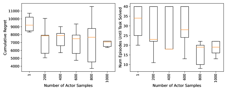
Figure 2: The effect of critic-guided random optimal action search (multiple shooting) on the performance of our PAC4SAC algorithm demonstrated on the cartpole swingup environment. Taking more samples reduces cumulative regret (left panel) and improves sample efficiency (right panel).

Table 2: The contribution of the critic training loss terms to performance. When used alone, the data fit term yields high cumulative regret. Both the catastrophic interference mitigation and overestimation correction terms bring performance improvement. The complete critic loss reaches the lowest cumulative regret and brings improved sample efficiency.

				Cartpole Swingup		Half Cheetah
	Data Fit	Catastrophic Interference Mitigation	Overestimation Correction	Cumulative Regret	Num Episodes Until Task Solved	Cumulative Regret	Num Episodes Until Task Solved
PAC4SAC	$\checkmark$	$\times$	$\times$	$6509.6\pm\color[rgb]{0.2,0.2,0.2}\scriptstyle 1454.1$	$24.6\pm\color[rgb]{0.2,0.2,0.2}\scriptstyle 5.9$	$182229.5\pm\color[rgb]{0.2,0.2,0.2}\scriptstyle 14365.9$	$250.0\pm\color[rgb]{0.2,0.2,0.2}\scriptstyle 0.0$
	$\checkmark$	$\checkmark$	$\times$	$5885.8\pm\color[rgb]{0.2,0.2,0.2}\scriptstyle 348.5$	$25.4\pm\color[rgb]{0.2,0.2,0.2}\scriptstyle 3.4$	$141634.7\pm\color[rgb]{0.2,0.2,0.2}\scriptstyle 21518.0$	$\bf 205.2\pm\color[rgb]{0.2,0.2,0.2}\scriptstyle 21.1$
	$\checkmark$	$\times$	$\checkmark$	$7065.0\pm\color[rgb]{0.2,0.2,0.2}\scriptstyle 990.5$	$\bf 17.0\pm\color[rgb]{0.2,0.2,0.2}\scriptstyle 2.0$	$153038.9\pm\color[rgb]{0.2,0.2,0.2}\scriptstyle 17313.9$	$211.6\pm\color[rgb]{0.2,0.2,0.2}\scriptstyle 21.1$
	$\checkmark$	$\checkmark$	$\checkmark$	$\bf 5722.1\pm\color[rgb]{0.2,0.2,0.2}\scriptstyle 348.4$	$22.0\pm\color[rgb]{0.2,0.2,0.2}\scriptstyle 5.1$	$\bf 132804.7\pm\color[rgb]{0.2,0.2,0.2}\scriptstyle 10801.1$	$223.6\pm\color[rgb]{0.2,0.2,0.2}\scriptstyle 14.6$

5 Discussion, Broader Impact, and Limitations

Our results demonstrate strong evidence in favor of the benefits of using the PAC Bayesian theory as a guideline for improving the performance of the actor-critic algorithms. Despite the demonstrated remarkable empirical performance, the tightness of the PAC Bayesian bound we used deserves dedicated investigation. Following Fard et al. (2012), we adopt one specific PAC Bayesian bound derived by Boucheron et al. (2005) due to its convenience for use in the Markov process setting. There may however be alternative approaches to bound the expectation of a Markov chain more tightly. Such theoretical considerations are topics for follow-up work. The sample efficiency improvement attained thanks to a PAC Bayes trained critic may be amplified even further by extending our findings to model-based and multi-step bootstrapping setups.

The strong empirical results of this work encourages exploration of venues beyond reinforcement learning, where the PAC Bayesian theory may be useful for training loss design. For instance, diffusion models (Berry and Berry, 2018) may derive PAC Bayesian loss functions to improve the notoriously unstable training schemes of deep generative models by semi-informative priors.

While our PAC4SAC shows consistent improvement over existing methods, it introduces additional hyperparameters such as the variance regularization coefficient, the prior distribution, and the number of shootings. Moreover, the need for multiple shooting at the action selection time increases computational complexity linear to the number of shootings. Reusing the same minibatch sample twice in expected variance calculation accelerates computation but is likely to induce bias to the estimator. While our method would still work if the term is calculated instead by resampling, this will increase the computational cost. Last but not least, the probabilistic layers of the critic network have the additional variance parameters to be learned.

Appendix A Appendix

A.1 Algorithm Pseudo-code

Algorithm 1 The PAC4SAC algorithm

0:  Polyak parameter $\tau\in(0,1)$, Learning rate $\eta>0$, Prior distribution $p_{pri}(\theta)$, Minibatch size $M>0$, Entropy coefficient $\alpha>0$, Regularization coefficient $\xi>0$

1:  $\mathcal{D}:=\emptyset,~{}~{}~{}~{}t:=0$ $\triangleright$ Initialize replay buffer and the time index

2:  $s_{0}:=$ env.reset()

3:  $a_{0}:=\arg\max_{a_{(1)},\ldots,a_{(S)}\sim\pi(a_{0}|s_{0})}\{(a_{(i)},Q_{\pi}^{\theta}(s_{0},a_{(i)}))|i=1,\ldots,S\}$ $\triangleright$ Multiple shooting

4:  $(r_{0},s_{1}):=$ env.step($a_{0}$) $\triangleright$ Take action

5:  $\mathcal{D}:=\mathcal{D}\cup(s_{0},a_{0},r_{0},s_{1})$ $\triangleright$ Store first observation into replay buffer

6:  repeat

7:     $a_{t}:=\arg\max_{a_{(1)},\ldots,a_{(S)}\sim\pi(a_{t}|s_{t})}\{(a_{(i)},Q_{\pi}^{\theta}(s_{t},a_{(i)}))|i=1,\ldots,S\}$ $\triangleright$ Multiple shooting

8:     $(r_{t},s_{t+1}):=$ env.step($a_{t}$) $\triangleright$ Take action

9:     $\mathcal{D}:=\mathcal{D}\cup(s_{t},a_{t},r_{t},s_{t+1})$ $\triangleright$ Store new observation into replay buffer

10:     $\widetilde{\mathcal{D}}:=\{(s_{t},a_{t},r_{t},s_{t+1},\widetilde{a}_{t+1})~{}|~{}(s_{t},a_{t},r_{t},s_{t+1})\sim\mathcal{D},~{}~{}\widetilde{a}_{t+1}\sim\pi(a_{t+1}|s_{t+1})$, $t=1,\ldots,M$} $\triangleright$ Sample batch and next actions

11:     $y_{t}\leftarrow r_{t}+\gamma Q_{\pi}^{\widetilde{\theta}}(s_{t+1},\widetilde{a}_{t+1})-\alpha\log\pi(\widetilde{a}_{t+1}|s_{t+1}),\quad\widetilde{\theta}_{t}\sim q(\theta;\phi^{\prime}),\quad\forall t=1,\ldots,M$ $\triangleright$ Calculate soft Bellman targets

12:     $q_{t}\leftarrow Q_{\pi}^{\widetilde{\theta}_{t}}(s_{t},a_{t}),\quad\widetilde{\theta}_{t}\sim q(\theta;\phi),\quad\forall t=1,\ldots,M$ $\triangleright$ Predict state-action values

13:     $\triangleright$ Build critic loss

$$L_{PAC4SAC}(\phi):=$$

$$~{}~{}~{}\frac{1}{M}\sum_{t=1}^{M}(q_{t}-y_{t})^{2}+\sqrt{\frac{D_{KL}(q(\theta;\phi)||p_{pri}(\theta))}{|\mathcal{D}|}}-\gamma\xi\left(\frac{1}{M}\sum_{t=1}^{M}q_{t}^{2}-\left(\frac{1}{M}\sum_{t=1}^{M}q_{t}\right)^{2}\right)$$

14:     $\phi\leftarrow\phi-\eta\nabla_{\phi}L_{PAC4SAC}(\phi)$ $\triangleright$ Policy evaluation

15:     $\pi\leftarrow\pi+\eta\nabla_{\pi}\Big{(}\frac{1}{M}\sum_{t=1}^{M}Q_{\pi}^{\widetilde{\theta}_{t}}(s_{t},\widetilde{a}_{t})\Big{)},\quad\widetilde{a}_{t}\sim\pi(a_{t}|s_{t}),\quad\widetilde{\theta}_{t}\sim q(\theta;\phi),\forall t=1,\ldots,M$ $\triangleright$ Policy improvement

16:     $\phi^{\prime}\leftarrow\tau\phi+(1-\tau)\phi^{\prime}$ $\triangleright$ Target critic update

17:     $s_{t}:=s_{t+1},\qquad t:=t+1$ $\triangleright$ Jump to next state

18:  until convergence

A.2 Prior Art

Actor-critic algorithms.

The Deep Deterministic Policy Gradient (DDPG) algorithm (Lillicrap et al., 2016) is among the pioneer work to adapt actor-critic algorithms to deep learning. The algorithm trains a critic to minimize the Bellman error and a deterministic actor to maximize the critic, following a simplified case of the policy gradient theorem. The Twin Delayed Deep Deterministic Policy Gradient (TD3) algorithm (Fujimoto et al., 2018) improves the robustness of DDPG by adopting twin critic networks backed up by Polyak averaging updated target copies. Trust region algorithms such as Relative Entropy Policy Search (REPS) (Peters et al., 2010), Trust Region Policy Optimization (TRPO) (Schulman et al., 2015), and PPO (Schulman et al., 2017) aim to explore while guaranteeing monotonic expected return improvement and maintaining training stability by restricting the policy updates via a KL divergence penalty between the policy densities before and after a parameter update. Fitted Policy Iteration (FPI) (Antos et al., 2008) is a variance reduced critic estimation method which finds near-optimal policy using a Vapnik-Chervonenkis crossing dimension technique in order to control the influence of variance term as a penalty factor. The Network Randomization method (Lee et al., 2019) enhances the generalization ability of RL agents by incorporating a randomized network that applies random perturbations to input observations which induces robustness to the policy-gradient algorithm by encouraging exploration.

Maximum entropy reinforcement learning.

Incorporation of the entropy of the policy distribution into the learning objective finds its roots in inverse reinforcement learning (Ziebart et al., 2008), which maintained its use also in modern deep inverse reinforcement learning applications Wulfmeier et al. (2015). The soft Q-learning algorithm (Haarnoja et al., 2017) uses the same idea to improve exploration in forward reinforcement learning. SAC (Haarnoja et al., 2018) extends the applicability of the framework to the off-policy setup by also significantly improving its stability and efficiency thanks to an actor training scheme provably consistent with a maximum entropy trained critic network. Among optimistic exploration algorithms, Seo et al. (2021) provides a sample efficient exploration method named RE3 for high-dimensional observation spaces, which estimates the state entropy using k-nearest neighbors in a low-dimensional embedding space. Another exploration method for high-dimensional environments with sparse rewards presented in (Zhang et al., 2021) provides a sample efficient exploration strategy by maximizing deviation from explored areas.

PAC Bayesian learning.

Introduced conceptually by Shawe-Taylor and Williamson (1997), PAC Bayesian analysis has been used by McAllester (1999, 2003) for stochastic model selection and its tightness has been improved by Seeger (2002) with application to Gaussian Processes (GPs). The use of PAC Bayesian bounds to training models while maintaining performance guarantees has raised attention since the pioneer work of Dziugaite and Roy (2017). Reeb et al. (2018) show how PAC Bayesian learning can be extended also to hyperparameter tuning. The first work to develop a PAC Bayesian bound for reinforcement learning is Fard and Pineau (2010). This bound has later on been extended by the same authors to continuous state spaces Fard et al. (2012). PAC Bayesian bounds start to be used in classical control problems for policy search (Veer and Majumdar, 2021), as well as for knowledge transfer (Majumdar, 2018; Farid and Majumdar, 2021). There is no work prior to ours that employs PAC Bayesian bounds for policy evaluation as part of an actor-critic algorithm.

A.3 Proof of Theorem 3.1

The lemma below shows that Theorem 3.1 defined originally in Fard et al. (2012) to build the relationship between the approximation error for the state-action function and the Bellman residual applies also to the soft Bellman operator. The rest of the proof of Theorem 3.1 directly follows.

Lemma A.3.1. For the squared weighted $L_{2}$ norm and Bellman operator defined as

$$T_{\pi}Q_{\pi}^{\theta}(s_{t},a_{t})=r(s_{t},a_{t})+\mathbb{E}_{p(s_{t+1}|s_{t},a_{t})\pi(a_{t+1}|s_{t+1})}[\gamma Q_{\pi}^{\theta}(s_{t+1},a_{t+1})-\log\pi(a_{t+1}|s_{t+1})],$$ (8)

the value approximation error is bounded as below:

$$\lVert Q_{\pi}^{\theta}(s_{t},a_{t})-Q_{\pi}(s_{t},a_{t})\rVert_{p_{\pi}(s_{t})\pi(a_{t}|s_{t})}^{2}\leq\frac{1}{(1-\gamma)^{2}}\lVert T_{\pi}Q_{\pi}^{\theta}(s_{t},a_{t})-Q_{\pi}^{\theta}(s_{t},a_{t})\rVert_{p_{\pi}(s_{t})\pi(a_{t}|s_{t})}^{2}.$$

Proof.

We have that

$$\lVert Q_{\pi}^{\theta} (s_{t},a_{t})-Q_{\pi}(s_{t},a_{t})\rVert_{p_{\pi}(s_{t})\pi(a_{t}|s_{t})}$$

$$=\lVert Q_{\pi}^{\theta}(s_{t},a_{t})-Q_{\pi}(s_{t},a_{t})+T_{\pi}Q_{\pi}^{\theta}(s_{t},a_{t})-T_{\pi}Q_{\pi}^{\theta}(s_{t},a_{t})\rVert_{p_{\pi}(s_{t})\pi(a_{t}|s_{t})}$$

$$\leq\lVert Q_{\pi}^{\theta}(s_{t},a_{t})-T_{\pi}Q_{\pi}^{\theta}(s_{t},a_{t})\rVert_{p_{\pi}(s_{t})\pi(a_{t}|s_{t})}+\lVert T_{\pi}Q_{\pi}^{\theta}(s_{t},a_{t})-Q_{\pi}(s_{t},a_{t})\rVert_{p_{\pi}(s_{t})\pi(a_{t}|s_{t})}\qquad\qquad$$

$$\leq\lVert Q_{\pi}^{\theta}(s_{t},a_{t})-T_{\pi}Q_{\pi}^{\theta}(s_{t},a_{t})\rVert_{p_{\pi}(s_{t})\pi(a_{t}|s_{t})}+\gamma\lVert Q_{\pi}^{\theta}(s_{t},a_{t})-Q_{\pi}(s_{t},a_{t})\rVert_{p_{\pi}(s_{t})\pi(a_{t}|s_{t})}.$$

Above the first inequality is attained via the triangle inequality and the second via the contraction inequality (Bertsekas and Tsitsiklis, 1996)

$$\lVert T_{\pi}Q_{\pi}(s_{t},a_{t})-Q_{\pi}(s_{t},a_{t})\rVert_{p_{\pi}(s_{t})\pi(a_{t}|s_{t})} \leq\gamma\|Q_{\pi}(s_{t},a_{t})-Q_{\pi}(s_{t},a_{t})\rVert_{p_{\pi}(s_{t})\pi(a_{t}|s_{t})}$$

that holds for any $Q_{\pi}$. Arranging the terms we get

$$\lVert Q_{\pi}^{\theta}(s_{t},a_{t})-Q_{\pi}(s_{t},a_{t})\rVert_{p_{\pi}(s_{t})\pi(a_{t}|s_{t})}\leq\frac{1}{1-\gamma}\lVert T_{\pi}Q_{\pi}^{\theta}(s_{t},a_{t})-Q_{\pi}^{\theta}(s_{t},a_{t})\rVert_{p_{\pi}(s_{t})\pi(a_{t}|s_{t})}.$$

Taking the square of both sides gives the desired result. ∎

The following PAC Bayes bound follows from Equation (5) of Fard et al. (2012).

Lemma A.3.2. Let $c_{1},c_{2}\in\mathbb{Z}^{+}$ be arbitrary constants, $p_{pri}$ and $q$ be prior and posterior measures respectively defined on $\Theta$, a set of observations $\mathcal{D}=\{(s_{t},a_{t},r_{t},s_{t+1})|t=1,\ldots,N\}$ following a Markov Decision Process $(\mathcal{S},\mathcal{A},p,p_{0},r,\gamma)$, then for any $N\in\mathbb{N}^{+}$ and $0<\delta<1$ it holds with probability greater than $1-\delta$ that:

$$\mathbb{E}_{q(\theta)}[R(\theta;\pi)]\leq\quad\mathbb{E}_{q(\theta)}[R_{N}(\theta;\pi,\mathcal{D})]+\sqrt{\frac{\log\left(\frac{c_{2}N}{c_{1}(r_{max}+|r_{min}|)^{2}\delta}\right)+D_{KL}(q(\theta)||p_{pri}(\theta))}{\frac{N}{(r_{max}+|r_{min}|)^{2}c_{1}}-1}}.$$

Using the below identity, which is a trivial result of the definition of variance

$$\lVert T_{\pi}Q_{\pi}^{\theta}(s_{t},a_{t})-Q_{\pi}^{\theta}(s_{t},a_{t})\rVert_{p_{\pi}(s_{t})\pi(a_{t}|s_{t})}^{2}=\mathbb{E}_{p_{\pi}(s_{t})\pi(a_{t}|s_{t})}\left[\left(T_{\pi}Q_{\pi}^{\theta}(s_{t},a_{t})-Q_{\pi}^{\theta}(s_{t},a_{t})\right)^{2}\right]$$

$$=R(\theta;\pi)-\mathbb{E}_{p_{\pi}(s_{t})\pi(a_{t}|s_{t})}\Bigg{[}r(s_{t},a_{t})+\gamma\mathbb{V}_{p(s_{t+1}|s_{t},a_{t})}\Big{[}\mathbb{E}_{\pi(a_{t+1}|s_{t+1})}[Q_{\pi}^{\theta}(s_{t+1},a_{t+1})]\Big{]}\Bigg{]}$$

we get

$$\mathbb{E}_{q(\theta)}\Big{[}\lVert T_{\pi}Q_{\pi}^{\theta}(s_{t},a_{t})-Q_{\pi}^{\theta}(s_{t},a_{t})\rVert_{p_{\pi}(s_{t})\pi(a_{t}|s_{t})}^{2}\Big{]}$$

$$\qquad=\lVert T_{\pi}Q_{\pi}^{\theta}(s_{t},a_{t})-Q_{\pi}^{\theta}(s_{t},a_{t})\rVert_{q(\theta)p_{\pi}(s_{t})\pi(a_{t}|s_{t})}^{2}$$

$$\qquad=\mathbb{E}_{q(\theta)}\left[R(\theta;\pi)-\mathbb{E}_{p_{\pi}(s_{t})\pi(a_{t}|s_{t})}\Big{[}r(s_{t},a_{t})+\gamma\mathbb{V}_{p(s_{t+1}|s_{t},a_{t})}\Big{[}\mathbb{E}_{\pi(a_{t+1}|s_{t+1})}[Q_{\pi}^{\theta}(s_{t+1},a_{t+1})]\Big{]}\Big{]}\right]$$

$$\qquad\leq\quad\mathbb{E}_{q(\theta)}[R_{N}(\theta;\pi,\mathcal{D})]+\sqrt{\frac{\log\left(\frac{c_{2}N}{c_{1}(r_{max}+|r_{min}|)^{2}\delta}\right)+D_{KL}(q(\theta)||p_{pri}(\theta))}{\frac{N}{(r_{max}+|r_{min}|)^{2}c_{1}}-1}}$$

$$\qquad\qquad-\mathbb{E}_{q(\theta)p_{\pi}(s_{t})\pi(a_{t}|s_{t})}\Bigg{[}r(s_{t},a_{t})+\gamma\mathbb{V}_{p(s_{t+1}|s_{t},a_{t})}\Big{[}\mathbb{E}_{\pi(a_{t+1}|s_{t+1})}[Q_{\pi}^{\theta}(s_{t+1},a_{t+1})]\Big{]}\Bigg{]}.$$

Lastly, applying in Lemma A.3.1 to the left hand side of the inequality above, we attain the desired result, which is a PAC Bayesian upper bound on the expected approximation error of the state-action value function, i.e. the critic, with respect to a distribution over its parameters: $||Q_{\pi}^{\theta}(s_{t},a_{t})-Q_{\pi}(s_{t},a_{t})||_{p_{\pi}(s_{t})\pi(a_{t}|s_{t})q(\theta)}^{2}$. The full statement of the theorem then reads as follows.

Theorem 3.1. Let $c_{1},c_{2}\in\mathbb{Z}^{+}$ be arbitrary constants, $p_{pri}$ and $q$ be prior and posterior measures respectively defined on $\Theta$, a set of observations $\mathcal{D}=\{(s_{t},a_{t},r_{t},s_{t+1})|t=1,\ldots,N\}$ following a Markov Decision Process $(\mathcal{S},\mathcal{A},p,p_{0},r,\gamma)$, then for any $N\in\mathbb{N}^{+}$ and $0<\delta<1$ it holds with probability greater than $1-\delta$ that:

$$||Q_{\pi}^{\theta}(s_{t},a_{t}) -Q_{\pi}(s_{t},a_{t})||_{p_{\pi}(s_{t})\pi(a_{t}|s_{t})q(\theta)}^{2}\leq$$

$$\frac{1}{(1-\gamma)^{2}}\Bigg{(}\mathbb{E}_{q(\theta)}[R_{N}(\theta;\pi,\mathcal{D})]+\sqrt{\frac{\log\left(\frac{c_{2}N}{c_{1}(r_{max}+|r_{min}|)^{2}\delta}\right)+D_{KL}(q(\theta)||p_{pri}(\theta))}{\frac{N}{(r_{max}+|r_{min}|)^{2}c_{1}}-1}}$$

$$\qquad-\mathbb{E}_{q(\theta)p_{\pi}(s_{t})\pi(a_{t}|s_{t})}\Bigg{[}r(s_{t},a_{t})+\gamma\mathbb{V}_{p(s_{t+1}|s_{t},a_{t})}\Big{[}\mathbb{E}_{\pi(a_{t+1}|s_{t+1})}[Q_{\pi}^{\theta}(s_{t+1},a_{t+1})]\Big{]}\Bigg{]}\Bigg{)}.$$

Appendix A.3.2: Proof of Theorem 3.2

Theorem 3.2. Let

$$\pi_{new}:=\arg\min_{\pi}D_{KL}\left(\pi(a_{t}|s_{t})\Bigg{|}\Bigg{|}\frac{\exp(Q_{\pi_{S}^{{old}}}(a_{t}|s_{t}))}{\int\exp(Q_{\pi_{S}^{{old}}}(a^{\prime}_{t}|s_{t})da^{\prime}}\right),$$

then $Q_{\pi_{S}^{new}}(s_{t},a_{t})\geq Q_{\pi_{S}^{old}}(s_{t},a_{t}),\forall(s_{t},a_{t})\in\mathcal{S}\times\mathcal{A}$.

Proof.

Denote $V_{\pi_{S}}(s_{t})=\mathbb{E}_{\pi(a_{t}|s_{t})}[Q_{\pi_{S}}(s_{t},a_{t})-\log\pi(a_{t}|s_{t})]$ and the optimization objective

$$J(\pi) :=D_{KL}\left(\pi(a_{t}|s_{t})\Bigg{|}\Bigg{|}\frac{\exp(Q_{\pi_{S}^{{old}}}(a_{t}|s_{t}))}{\int\exp(Q_{\pi_{S}^{{old}}}(a^{\prime}_{t}|s_{t})da^{\prime}}\right)$$

$$=\mathbb{E}_{\pi(a_{t}|s_{t})}[\log\pi(a_{t}|s_{t})-Q_{\pi_{S}^{{old}}}(s_{t},a_{t})]+\mathrm{const}.$$

Since $J(\pi_{new})\leq J(\pi_{S}^{old})$, we have

$$\mathbb{E}_{\pi_{new}(a_{t}|s_{t})}[Q_{\pi_{S}^{{old}}}(s_{t},a_{t}) -\log\pi_{new}(a_{t}|s_{t})]$$

$$\geq\mathbb{E}_{\pi_{S}^{{old}}(a_{t}|s_{t})}[Q_{\pi_{S}^{{old}}}(s_{t},a_{t})-\log\pi_{S}^{{old}}(a_{t}|s_{t})]=V_{\pi_{S}^{{old}}}(s_{t}).$$

Taking $S$ action samples from $\pi_{new}$ and choosing the sample that maximizes the state-action value

$$a_{t}^{*} =\arg\max_{a_{(1)},\ldots,a_{(S)}\sim\pi_{{new}}(a_{t}|s_{t})}\{(a_{(i)},Q_{\pi_{{new}}}(s_{t},a_{(i)}))|i=1,\ldots,S\}$$

we will have

$$\mathbb{E}_{\pi_{new}(a_{t}|s_{t})}[Q_{\pi_{S}^{{old}}}(s_{t},a_{t})-\log\pi_{new}(a_{t}|s_{t})]\leq Q_{\pi_{S}^{{old}}}(s_{t},a_{t}^{*})-\mathbb{E}_{\pi_{new}(a_{t}|s_{t})}[\log\pi_{new}(a_{t}|s_{t})].$$

Plugging this inequality into the Bellman equation and expanding it recursively, we get

$$Q_{\pi_{S}^{old}} (s_{t},a_{t})=r(s_{t},a_{t})+\gamma\mathbb{E}_{p(s_{t+1}|s_{t},a_{t})}[V_{\pi_{S}^{old}}(s_{t})]$$

$$\leq r(s_{t},a_{t})+\gamma\mathbb{E}_{p(s_{t+1}|s_{t},a_{t})\pi_{new}(a_{t+1}|s_{t+1})}[Q_{\pi_{S}^{old}}(s_{t+1},a_{t+1})-\log\pi_{new}(a_{t+1}|s_{t+1})]$$

$$\leq r(s_{t},a_{t})+\gamma\mathbb{E}_{p(s_{t+1}|s_{t},a_{t})}[Q_{\pi_{S}^{{old}}}(s_{t+1},a_{t+1}^{*})-\mathbb{E}_{\pi_{new}(a_{t+1}|s_{t+1})}[\log\pi_{new}(a_{t+1}|s_{t+1})]]$$

$$~{}~{}\vdots$$

$$\leq Q_{\pi_{S}^{new}}(s_{t},a_{t}).$$

∎

A.4 Experimental details

We implement all experiments with the PyTorch (Paszke et al., 2019) version $1.13.1$.

Environments.

For experiments, we use PyBullet Gymperium library. We choose the environment handle InvertedPendulumSwingupPyBulletEnv-v0 for Cartpole Swingup, HalfCheetahMuJoCoEnv-v0 for Half Cheetah, AntMuJoCoEnv-v0 for Ant, and HumanoidMuJoCoEnv-v0 for Humanoid.

Hyper-parameters.

We use Adam optimizer (Kingma and Ba, 2015) with a learning rate of $0.001$ for all architectures. We set the length of experience replay as $25000$ and batch size as $32$. For PAC4SAC we set the regularization parameter to $\xi=0.01$. For SAC-NR, we raise the network perturbation coefficient denoted in Lee et al. (2019) as $\alpha$ from $0.1$ to $0.5$, which gave a significant improvement in model performance to the favor of this baseline. We set $\beta=0.002$ as suggested in the original paper.

Architectures.

We use the same architecture for all the environments and models in comparison. There are two main architectures which are actor and critic and we provide the details of the architectures in Table 3.

Actor				Critic
SAC-NR	SAC SAC-FPI PAC4SAC	DDPG		SAC SAC-NR SAC-FPI DDPG	PAC4SAC
NR-Linear($d_{s}$, $d_{s}$)	n/a	n/a
Linear($d_{s}$, 256) LayerNorm(256) Silu()				Linear($d_{s}$ + $d_{a}$, 256) LayerNorm(256) Silu()
Linear(256, 256) LayerNorm(256) Silu()				Linear(256, 256) LayerNorm(256) Silu()
Linear(256, 256) LayerNorm(256) Silu()				Linear(256, 256) LayerNorm(256) Silu()
Linear(256, 2$\times d_{a}$, $\theta$)		Linear(256, $d_{a}$)		Linear(256, 1)	GaussLinear(256, 1)
SquashedGaussian(2$\times d_{a}$, $d_{a}$)		Tanh()

Table 3: Architecture details based on environments. The SquashedGaussian module implements a Gaussian head that uses the first $d_{a}$ of its inputs as the mean and the second $d_{a}$ as the variance of a heteroscedastic normal distribution. The GaussLinear module implements a fully connected layer with weights that follow independent normal distributions. The NR-Linear is a randomized linear layer as in Lee et al. (2019).

References

• Bertsekas and Tsitsiklis (1996) Bertsekas, D.; Tsitsiklis, J. Neuro-dynamic programming; 1996.
• Peters et al. (2010) Peters, J.; Mulling, K.; Altun, Y. Relative entropy policy search. AAAI. 2010.
• Schulman et al. (2015) Schulman, J.; Levine, S.; Abbeel, P.; Jordan, M.; Moritz, P. Trust region policy optimization. ICML. 2015.
• Lillicrap et al. (2016) Lillicrap, T.; Hunt, J.; Pritzel, A.; Heess, N.; Erez, T.; Tassa, Y.; Silver, D.; Wierstra, D. Continuous control with deep reinforcement learning. ICLR. 2016.
• Schulman et al. (2017) Schulman, J.; Wolski, F.; Dhariwal, P.; Radford, A.; Klimov, O. Proximal policy optimization algorithms. arXiv preprint arXiv:1707.06347 2017,
• Haarnoja et al. (2018) Haarnoja, T.; Zhou, A.; Abbeel, P.; Levine, S. Soft Actor-Critic: Off-policy maximum entropy deep reinforcement learning with a stochastic actor. ICML. 2018.
• Fujimoto et al. (2018) Fujimoto, S.; Hoof, H.; Meger, D. Addressing function approximation error in actor-critic methods. ICML. 2018.
• Shawe-Taylor and Williamson (1997) Shawe-Taylor, J.; Williamson, R. A PAC analysis of Bayesian estimator. COLT. 1997.
• McAllester (1999) McAllester, D. PAC-Bayesian model averaging. COLT. 1999.
• Alquier (2021) Alquier, P. User-friendly introduction to PAC-Bayes bounds. arXiv preprint arXiv:2110.11216 2021,
• Dziugaite and Roy (2017) Dziugaite, G.; Roy, D. Computing non-vacuous generalization bounds for deep (stochastic) neural networks with many more parameters than training data. UAI. 2017.
• Haußmann et al. (2021) Haußmann, M.; Gerwinn, S.; Look, A.; Rakitsch, B.; Kandemir, M. Learning partially known stochastic dynamics with empirical PAC Bayes. AISTATS. 2021.
• Fard et al. (2012) Fard, M.; Pineau, J.; Szepesvári, C. PAC-Bayesian policy evaluation for reinforcement learning. AISTATS. 2012.
• Van Hasselt et al. (2016) Van Hasselt, H.; Guez, A.; Silver, D. Deep reinforcement learning with double q-learning. AAAI. 2016.
• Kearns and Vazirani (1994) Kearns, M.; Vazirani, U. An introduction to computational learning theory; MIT press, 1994.
• Thrun and Schwartz (1993) Thrun, S.; Schwartz, A. Issues in using function approximation for reinforcement learning. Proceedings of the Fourth Connectionist Models Summer School. 1993.
• Pritzel et al. (2017) Pritzel, A.; Uria, B.; Srinivasan, S.; Badia, A.; Vinyals, O.; Hassabis, D.; Wierstra, D.; Blundell, C. Neural episodic control. ICML. 2017.
• Vapnik (1999) Vapnik, V. The nature of statistical learning theory; Springer science & business media, 1999.
• Chua et al. (2018) Chua, K.; Calandra, R.; McAllister, R.; Levine, S. Deep reinforcement learning in a handful of trials using probabilistic dynamics models. NeurIPS 2018,
• Hafner et al. (2019) Hafner, D.; Lillicrap, T.; Fischer, I.; Villegas, R.; Ha, D.; Lee, H.; Davidson, J. Learning latent dynamics for planning from pixels. ICML. 2019.
• Hafner et al. (2020) Hafner, D.; Lillicrap, T.; Ba, J.; Norouzi, M. Dream to control: Learning behaviors by latent imagination. ICLR. 2020.
• Levine (2013) Levine, V., S.and Koltun Guided policy search. ICML. 2013.
• Sutton and Barto (2018) Sutton, R.; Barto, A. Reinforcement learning: An introduction; MIT press, 2018.
• Antos et al. (2008) Antos, A.; Szepesvári, C.; Munos, R. Learning near-optimal policies with Bellman-residual minimization based fitted policy iteration and a single sample path. Machine Learning 2008,
• Lee et al. (2019) Lee, K.; Lee, K.; Shin, J.; Lee, H. Network randomization: A simple technique for generalization in deep reinforcement learning. ICLR. 2019.
• Coumans and Bai (2016–2019) Coumans, E.; Bai, Y. PyBullet: a Python module for physics simulation for games, robotics and machine learning. http://pybullet.org, 2016–2019.
• Brockman et al. (2016) Brockman, G.; Cheung, V.; Pettersson, L.; Schneider, J.; Schulman, J.; Tang, J.; Zaremba, W. OpenAI Gym. arXiv preprint arXiv:1606.01540 2016,
• Ellenberger (2018–2019) Ellenberger, B. PyBullet Gymperium. https://github.com/benelot/pybullet-gym, 2018–2019.
• Boucheron et al. (2005) Boucheron, S.; Bousquet, O.; Lugosi, G. Theory of classification: A survey of some recent advances. ESAIM 2005,
• Berry and Berry (2018) Berry, F.; Berry, W. Innovation and diffusion models in policy research. Theories of the policy process 2018,
• Ziebart et al. (2008) Ziebart, B.; Maas, A.; Bagnell, J.; Dey, A., et al. Maximum entropy inverse reinforcement learning. AAAI. 2008.
• Wulfmeier et al. (2015) Wulfmeier, M.; Ondruska, P.; Posner, I. Maximum entropy deep inverse reinforcement learning. arXiv preprint arXiv:1507.04888 2015,
• Haarnoja et al. (2017) Haarnoja, T.; Tang, H.; Abbeel, P.; Levine, S. Reinforcement learning with deep energy-based policies. ICML. 2017.
• Seo et al. (2021) Seo, Y.; Chen, L.; Shin, J.; Lee, H.; Abbeel, P.; Lee, K. State entropy maximization with random encoders for efficient exploration. ICML 2021,
• Zhang et al. (2021) Zhang, T.; Rashidinejad, P.; Jiao, J.; Tian, Y.; Gonzalez, J. E.; Russell, S. Made: Exploration via maximizing deviation from explored regions. NeurIPS 2021,
• McAllester (2003) McAllester, D. PAC-Bayesian stochastic model selection. Machine Learning 2003,
• Seeger (2002) Seeger, M. PAC-Bayesian generalisation error bounds for Gaussian process classification. JMLR 2002,
• Reeb et al. (2018) Reeb, D.; Doerr, A.; Gerwinn, S.; Rakitsch, B. Learning Gaussian processes by minimizing PAC-Bayesian generalization bounds. NeurIPS 2018,
• Fard and Pineau (2010) Fard, M.; Pineau, J. PAC-Bayesian model selection for reinforcement learning. NeurIPS 2010,
• Veer and Majumdar (2021) Veer, S.; Majumdar, A. Probably approximately correct vision-based planning using motion primitives. CoRL. 2021.
• Majumdar (2018) Majumdar, M., A.and Goldstein PAC-Bayes Control: Synthesizing Controllers that Provably Generalize to Novel Environments. CoRL. 2018.
• Farid and Majumdar (2021) Farid, A.; Majumdar, A. Generalization bounds for meta-learning via PAC-Bayes and uniform stability. NeurIPS 2021,
• Paszke et al. (2019) Paszke, A. et al. PyTorch: An Imperative Style, High-Performance Deep Learning Library. NeurIPS 2019,
• Kingma and Ba (2015) Kingma, D.; Ba, J. Adam: A method for stochastic optimization. ICLR. 2015.