Day-timescale variability in the radio light curve of the Tidal Disruption Event AT2022cmc: confirmation of a highly relativistic outflow

Abstract

Tidal disruption events (TDEs) are transient, multi-wavelength events in which a star is ripped apart by a supermassive black hole. Observations show that in a small fraction of TDEs, a short-lived, synchrotron emitting jet is produced. We observed the newly discovered TDE AT2022cmc with a slew of radio facilities over the first 100 days after its discovery. The light curve from the AMI–LA radio interferometer shows day-timescale variability which we attribute to a high brightness temperature emitting region as opposed to scintillation. We measure a brightness temperature of 2$\times$10¹⁵ K, which is unphysical for synchrotron radiation. We suggest that the measured high brightness temperature is a result of relativistic beaming caused by a jet being launched at velocities close to the speed of light along our line of sight. We infer from day-timescale variability that the jet associated with AT2022cmc has a relativistic Doppler factor of at least 16, which corresponds to a bulk Lorentz factor of at least 8 if we are observing the jet directly on axis. Such an inference is the first conclusive evidence that the radio emission observed from some TDEs is from relativistic jets because it does not rely on an outflow model. We also compare the first 100 days of radio evolution of AT2022cmc with that of the previous bright relativistic TDE, Swift J1644, and find a remarkable similarity in their evolution.

1 Introduction

Multiple wide-field radio surveys have demonstrated that up to 30% of the radio sky is variable when observing at centimeter wavelengths (Bolton et al., 2006; Ofek et al., 2011; Bannister et al., 2011; Murphy et al., 2013, 2017; Sarbadhicary et al., 2021). Some variability is extrinsic, a result of scintillation, the scattering of radio waves by free electrons in the interstellar medium resulting in random flux modulations. Variability can also be intrinsic, a result of physical changes within the emitting region that can give clues to the nature of the source. A good example of this is observed in radio data sets of blazars (persistently accreting supermassive black holes (SMBHs) that launch outflows pointing towards Earth) which are highly variable and very luminous (Ulrich et al., 1997; Mundell et al., 2009). These characteristics are indicative of a highly relativistic outflow with a compact emitting region.

Blazars are not the only systems to produce jets, and not all jets are persistent: many stellar-mass black hole systems produce transient jets e.g. gamma-ray bursts or X-ray binaries (Rhodes et al., 2020; Fender et al., 2004; Bright et al., 2020). In the most energetic systems, the kinetic energy required for such an outflow is so high that the radiation must originate from a highly collimated jet as opposed to a spherical outflow (Mochkovitch et al., 1993; Sari et al., 1999; Mooley et al., 2018). The presence of a relativistic jet may be inferred by the detection of superluminal motion/expansion or the presence of a high brightness temperature component as a result of Doppler boosting (also known as relativistic beaming). Doppler boosting occurs when outflowing material is moving at velocities close to the speed of light (i.e. with high bulk Lorentz factors) and close to the observer’s line of sight making it appear more luminous than in the rest frame of the material.

If a star passes too close to a SMBH, the tidal forces of the SMBH can overcome the self-gravity keeping the star together and pull it apart creating a tidal disruption event (TDE; Rees, 1988). Approximately half of the disrupted material is thought to be lost while the other half falls back and is accreted onto the SMBH. In a small fraction of TDEs, the radiation at all wavelengths is dominated by luminous non-thermal emission thought to be produced by a jet. These systems are called relativistic TDEs. The most well-studied relativistic TDE to date is Swift J1644+57 which was first discovered due to a bright gamma-ray flash followed by a luminous, variable and decaying X-ray counterpart (Bloom et al., 2011; Burrows et al., 2011). A bright radio counterpart of Swift J1644+57 has been detected at low frequencies for the past decade and modelled as a narrow, highly relativistic jet pointed towards Earth (Bloom et al., 2011; Berger et al., 2012; Zauderer et al., 2013; Wang et al., 2014; Mimica et al., 2015; Eftekhari et al., 2018). The presence of a jet would be directly confirmed upon either the detection of superluminal motion/expansion (Yang et al., 2016) or the presence of a high brightness temperature as a result of Doppler boosting, but no such evidence has yet been found.

ZTF22aaajecp is a panchromatic transient discovered by the Zwicky Transient Facility on 2022 Feb 11 10:42 UT (MJD 59621.4458, $T_{0}$, Andreoni et al., 2022b) and registered on the Transient Name Server as AT2022cmc. The optical light curve shows a fast decay ($>$1 mag/day) until day 10 post-discovery when it settled into a plateau between 21 and 22 magnitudes (r-band, Pankov et al., 2022; Dimple et al., 2022; Cenko et al., 2022; Fulton et al., 2022). Early optical spectroscopy detected interstellar medium absorption from a likely host galaxy at $z=1.193$ (Tanvir et al., 2022). AT2022cmc is over four times more distant than Swift J1644+57 (assuming $H_{0}$ = 70 km s^-1 Mpc^-1 and $\Omega_{\textrm{M}}$ = 0.3, Levan et al., 2011). Rapid radio, sub-mm, and X-ray follow-up observations were also performed and bright counterparts were detected in all bands (e.g. Perley et al., 2022; Alexander et al., 2022; Dobie et al., 2022; Yao et al., 2022b; Pasham et al., 2022c). The high X-ray luminosity, hour-timescale variability and spectra from NICER and NuSTAR (Han et al., 2022; Yao et al., 2022a; Pasham et al., 2022b) indicated that AT2022cmc is a relativistic TDE, the first to be discovered in over a decade (Bloom et al., 2011; Cenko et al., 2012; Brown et al., 2015).

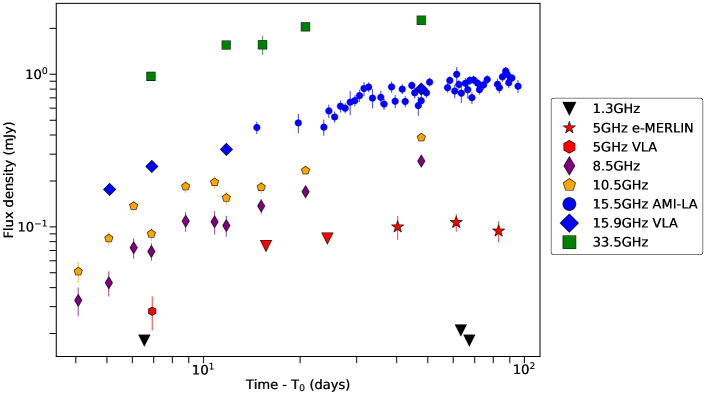
Figure 1: The radio light curve of AT2022cmc, combining the observations presented in this work at 3$\sigma$ upper limits at 1.3 GHz (black downwards facing triangles), e–MERLIN upper limits and detections at 5 GHz as red downwards facing triangles and stars, respectively) and 15.5 GHz detections and upper limits shown as blue circles and downwards facing triangles, respectively. Also shown are detections at 5 (red hexagons), 8.5 (purple narrow diamonds), 10 (gold pentagons), 15.9 (blue wide diamonds) and 33.5 GHz (green squares) from the VLA (Andreoni et al., 2022a). The 15.5 GHz light curve shows clear evidence of inter-observation variability. There is also evidence of variability at 10.5 GHz.

2 Methods

2.1 Observations

We obtained radio observations of AT2022cmc through guaranteed and rapid response time on the Arcminute Microkelvin Imager Large Array (AMI-LA), enhanced – Multi-Element Radio Linked Interferometer Network (e–MERLIN) and MeerKAT radio telescopes.

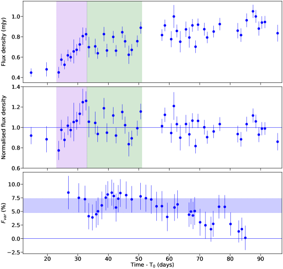
Figure 2: a: The AMI–LA 15.5 GHz light curve of AT2022cmc. The fractional variability is 16.5$\pm$1.3%. b: the 15.5 GHz light curve normalised by dividing through by a single power law fit to the data. The fractional variability of the whole normalised light curve is 6.1$\pm$1.3%. c: the fractional variability of AT2022cmc at 15.5 GHz as a function of time: each data point is the fractional variability of 15 days of observations plotted at the time average of those 15 days. The blue-shaded region is the time average fractional variability for the whole observing campaign. The purple and green shaded regions refer to the periods of ten-day and one-day variability.

2.1.1 AMI–LA

Observations with AMI–LA (Zwart et al., 2008; Hickish et al., 2018) started on 2022 February 26^th 00:40 UT (14.6 days after the initial discovery). For each observation 3C 286 was used as both the interleaved phase calibrator and to set the absolute flux scale. We use the custom pipeline reduce_dc (e.g. Perrott et al. 2013) to flag instrumental issues, calibrate the bandpass response of the array, correct for atmospheric temperatures, and solve for phases on the interleaved calibrator which were then applied to the target field. Because 3C 286 was also used as the complex gain calibrator, we reinitialized the sky-model for 3C 286 from the Perley-Butler 2017 standard (Perley & Butler, 2017) and solved for complex gains (both amplitudes and phases) with a solution interval of 600 s, deriving solutions for each of the eight frequency channels. We then image all observations for both fields using the casa task clean, and measure the flux density of 3C 286 and AT2022cmc using imfit. The resulting flux density was measured for 3C 286 is stable to better than 1.

2.1.2 e–MERLIN

We obtained Rapid Response Time observations (PI: Rhodes, RR13002) of AT2022cmc with e–MERLIN beginning with an initial epoch at 5 GHz on 2022 February 27^th 02:30 UT (15.7 days) with follow-up observations every three weeks. e–MERLIN data are reduced using a casa-based (Version 5.8.0) pipeline (Moldon, 2021). The pipeline averages, flags for radio frequency interference, calibrates and images the data. We do not detect the 5 GHz in the first two epochs. From 40 days onwards, a point source at around 100$\mu$Jy was persistently detected.

2.1.3 MeerKAT

Observations with MeerKAT were awarded through an open-time call for proposals (PI: Rhodes, MKT-20185). Three observations were made over the first 100 days, each at 1.28 GHz with a bandwidth of 0.856 GHz. MeerKAT data are reduced using oxkat, a series of semi-automated python scripts (Heywood, 2020). The scripts flag and calibrate the data using standard procedures in casa (McMullin et al., 2007) then images are made using wsclean (Offringa et al., 2014). A round of phase-only self-calibration is also performed. We do not detect any radio emission at the position of AT2022cmc in any of the three observations reported here.

2.2 Variability and brightness temperature calculations

To interpret the observations we have made of AT2022cmc, we calculate the brightness temperature using different variability timescales. Here, we present the fractional root mean square (rms) variability which is required to check whether any variability observed is statistically significant using the method from Vaughan et al. (2003). Then we demonstrate how to use a given variability timescale to calculate the brightness temperature and from there the relativistic Doppler factor.

The fractional rms variability examines the variability that is in excess of the contribution from the uncertainties associated with the measured flux densities. The fractional variability is given by

$$F_{\mathrm{var}}=\sqrt{\frac{S^{2}-\overline{\sigma_{\mathrm{err}}^{2}}}{\bar{S_{\nu}}^{2}}}$$ (1)

where the variance is

$$S^{2}=\frac{1}{N-1}\sum_{i=1}^{N}\left(S_{\nu,i}-\bar{S_{\nu}}\right)^{2}$$ (2)

and the mean error is,

$$\overline{\sigma_{\mathrm{err}}^{2}}=\frac{1}{N}\sum_{i=1}^{N}\sigma_{\mathrm{err},i}^{2}\text{. }$$ (3)

where $\bar{S_{\nu}}$ is the mean flux density and $N$ is the number of data points. The uncertainty associated with the fractional variability is given by:

$$\operatorname{err}\left(F_{\mathrm{var}}\right)=\sqrt{\left\{\sqrt{\frac{1}{2N}}\cdot\frac{\overline{\sigma_{\mathrm{err}}^{2}}}{\bar{x}^{2}F_{\mathrm{var}}}\right\}^{2}+\left\{\sqrt{\frac{\overline{\sigma_{\mathrm{err}}^{2}}}{N}}\cdot\frac{1}{\bar{x}}\right\}^{2}}$$ (4)

Equations 1 and 4 are used to calculate whether the variability observed in the light curve is real and statistically significant. We consider any F_var value greater than three times its associated uncertainty, $\operatorname{err}\left(F_{\mathrm{var}}\right)$ as statistically significant.

If the observed variability is real, we can calculate the brightness temperature of a radio source starting with:

$$T_{B}=\frac{S_{\nu}c^{2}}{2k_{B}\Omega\nu^{2}}$$ (5)

where $\Omega=R^{2}/D_{A}^{2}$, c is the speed of light, k_B is the Boltzmann constant, $\theta$ is the projected size of the source on the sky, $\nu$ is the observing frequency, $D_{A}$ is the angular diameter distance (i.e. the comoving distance: $D/(1+z)$ or the luminosity distance $D_{L}/(1+z)^{2}$) and $R$ is the radius of the source (Longair, 2011). All of the above variables are observable except for the radius ($R$), which can be inferred from an observed variability timescale: $R=c\Delta t_{\textrm{var}}/(1+z)$. Substituting these values into Equation 5 gives (Wagner & Witzel, 1995):

$$T_{B}=\frac{S_{\nu}D_{L}^{2}}{2k_{B}\nu^{2}t_{\textrm{var}}^{2}(1+z)^{2}}$$ (6)

Brightness temperatures above 10¹² K are not possible from synchrotron radiation (Kellermann & Pauliny-Toth, 1969). Above 10¹² K, the emitting region undergoes significant Compton cooling so that the brightness temperature drops back below 10¹² K, called the inverse-Compton catastrophe. Some incoherent transients have brightness temperatures above 10¹² K, such as gamma-ray bursts, where the cause of the high brightness temperatures is most likely relativistic beaming. Therefore, any brightness temperature measurements above 10¹² K must originate from radiation that is strongly beamed into our line of sight.

We use the brightness temperature measurements to infer the relativistic Doppler factor by substituting the following into Equation 6: $S_{\nu}=I_{\nu}\Omega$, $\nu=\nu^{\prime}/(1+z)$, the angular radius $\theta=(\delta_{\textrm{var}}c\Delta t_{\textrm{var}})/(D_{A}(1+z))$, and I_$\nu$/$\nu^{3}$ = I^′_$\nu$/$\nu^{\prime 3}$. Equation 6 can be rearranged to obtain the Doppler factor in terms of the observed brightness temperature (T_var) and a given rest frame temperature ($\textrm{T}^{\prime}_{\textrm{var}}$):

$$\delta_{\textrm{var}}=\sqrt[3]{(1+z)\frac{T_{\textrm{var}}}{T_{\textrm{var}}^{\prime}}}=\frac{1}{\Gamma(1-\beta\cos{\phi})}$$ (7)

where $\Gamma$ is the bulk Lorentz factor, $\beta$ is the velocity of the outflow material as a fraction of the speed of light and $\phi$ is the angle of the outflow to the line of sight. A result of Doppler boosting is that radiation is beamed into a cone within an opening angle, $\phi\approx 1/\Gamma$. For the work presented in this paper, we assume a rest frame brightness temperature of T^′_var = 10¹² K. However, it is possible that the rest frame temperature is considerably lower (e.g. Readhead, 1994; Lähteenmäki et al., 1999). From Equation 7, one can see that by decreasing T^′_var, the Doppler factor we infer would increase. Therefore, the Doppler factors we present in this work are lower limits.

3 Results

Figure 1 shows radio light curves from MeerKAT (1.3 GHz Jonas & MeerKAT Team, 2016), e–MERLIN (5 GHz) and AMI–LA (15.5 GHz) along with data points at 5, 8.5, 10.5, 15.9 and 33.5 GHz from the Karl G. Jansky Very Large Array (Andreoni et al., 2022a). In all bands (except 1.3 GHz, where AT2022cmc was not detected), the light curves show a slow rise over the duration of the respective observing campaigns. A radio counterpart was first detected with the AMI–LA from 14 days post-discovery (Sfaradi et al., 2022) and at 5 GHz with e–MERLIN at 40 days post-discovery. The high time cadence of the 15.5 GHz AMI–LA light curve shows day-timescale variability with an underlying slowly rising light curve.

To parameterize and understand the short timescale variations occurring within the radio emitting region as observed at 15.5 GHz we use the fractional variability. The fractional variability examines the variability that is in excess of the contribution from the uncertainties associated with the measured flux densities (Vaughan et al., 2003).

We measure a fractional variability of 16.5$\pm$1.3 % for the whole 15.5 GHz data set which considers both the underlying long-term flux density increase as well as the day-to-day variability. In order to determine if the short timescale variability is real, we fit a power law to the 15.5 GHz light curve (shown in Figure 2a) and divide the light curve data by the fit (Figure 2b) and obtain an excess variability of AT2022cmc is 6.1$\pm$1.3 %.

The observed variability is unlikely to be a result of scintillation at 15.5 GHz. For the position of AT2022cmc on the sky, the AMI–LA observing band is firmly in the weak scintillation regime (Cordes & Lazio, 2002). Any effects due to weak scintillation would cause variability on a timescale of approximately 1 hour with an amplitude of about 30% (Goodman, 1997). We measure no statistically significant variability on this timescale.

Given that it is unlikely that scintillation is the origin of the observed variability, it is possible that it originates from the TDE. A significant contribution ($\sim$ one third) to the fractional variability measurement originates from the data points between 23 and 33 days post-discovery where the flux density increases by 50% over 10 days (the highlighted purple region in Figure 2). A variability timescale ($\Delta t$) of 10 days corresponds to a very small emission region ($c\Delta t/(1+z)$) of $\lesssim$ 1.2$\times$10¹⁶ cm and a high brightness temperature of (2.0$\pm$0.4)$\times$10¹³ K.

From the brightness temperature of (2.0$\pm$0.4)$\times$10¹³ K, we use Equation 7, and $\textrm{T}_{\textrm{var}}^{\prime}$ = 10¹² K, to derive a Doppler factor of 4. There are two other rest frame brightness temperature limits that are often used in the literature: 2$\times$10¹¹ K (Sincell & Krolik, 1994) and 5$\times$10¹⁰ K (Readhead, 1994). By using these other values in our calculations, we obtain Doppler factors of 6 and 10, respectively. The dotted blue lines in Figure 3 shows the allowed values of $\Gamma$ and $\phi$ for three values of $\delta_{\textrm{var}}$ quoted above.

Between days 33 and 51 post-discovery (the green highlighted region in Figure 2), the AMI–LA light curve shows evidence of day-timescale variability. Shorter timescale variability corresponds to an even higher brightness temperature of (2.0$\pm$0.4)$\times$10¹⁵ K. We calculate values of $\delta_{\textrm{var}}$ to be 16, 27 and 30, for T^′_var = 10¹², 2$\times$10¹¹ K and 5$\times$10¹⁰ K, respectively (Sincell & Krolik, 1994; Readhead, 1994). All three values are marked by solid blue lines on Figure 3.

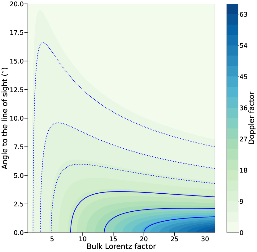
Figure 3: A contour plot showing the relativistic Doppler factor ($\delta_{\textrm{var}}$) as a function of angle to the line of sight and bulk Lorentz factor. The solid blue lines correspond to Doppler factors calculated from the day-timescale variability using rest frame brightness temperatures of 10¹², 2$\times$10¹¹ and 5$\times$10¹⁰ K. The dotted lines are the Doppler factors from the variability timescale of 10 days using the same three rest frame brightness temperatures.

Given the consistently high cadence data over the first 100 days after the TDE discovery, we can also search for changes in variability amplitude. Figure 2(c) shows the percentage fractional variability as a function of time using bins of 15 days. There is significant variability for the first 70 days after which the epoch-to-epoch variability ceases. There is no evidence in the data to link the reduction in variability to any spectral index variations. For the first 100 days, we measure a spectral index of 1.9$\pm$0.1, consistent with what is expected from self-absorbed synchrotron emission.

4 Discussion

Using model-independent analysis, from the Doppler factor calculation (Equation 7), we infer from day-timescale variability, that the bulk Lorentz factor of the outflowing material $\gtrsim$8 for a jet that is pointing directly towards Earth, i.e. the angle to the line of sight is zero degrees. Pasham et al. (2022a) also inferred a slightly higher bulk Lorentz factor through SED modelling. We also find that after the first 70 days post-discovery that there is a reduction in variability. This decrease could reflect a reduction in mass accretion rate (Rees & Meszaros, 1994; Malzac, 2013), or an intrinsic reduction of variability at the shock front.

In order to produce such a highly relativistic outflow, vast amounts of kinetic energy are required, so much so that the observed emission cannot originate from a spherical outflow. Andreoni et al. (2022a) used the X-ray emission to estimate an isotropic equivalent kinetic energy of $\approx 10^{53-54}$ erg. For an estimate of $10^{54}$ erg, at least 20 M_$\odot$ of material is required (by assuming an optimistic efficiency of 10% and considering that 50% of the material will not be accreted on to the SMBH) to produce the observed emission if the outflow is isotropic. This problem is alleviated if instead the outflow is collimated into a jet-like outflow and beamed into our line of sight.

Evidence of relativistic outflows has been found in many classes of systems, both galactic and extragalactic. Using Very Long Baseline Interferometry (e.g. Pearson et al., 1981; Unwin et al., 1985; Jorstad et al., 2001) and multi-wavelength monitoring programs (e.g. Liodakis et al., 2017), Doppler factors as high as those shown in Figure 3 have been found in blazars. Gamma-ray bursts, some of the most powerful explosions known, also require high bulk Lorentz factors of at least 100 (Zou & Piran, 2010; Ghirlanda et al., 2018). High angular resolution observations in multiple bands support the requirement for high launch Lorentz factors where gamma-ray burst jets have Lorentz factors of around 5, at tens to hundreds of days post-burst (Taylor et al., 2004; Mooley et al., 2022). We note that, in the case of gamma-ray bursts, it is often assumed that the angle to the line of sight is zero and Lorentz factors are quoted instead of Doppler factors.

Within the Milky Way, X-ray binaries have a larger range of Doppler factors. The average jet angle to the line of sight is around 60^$\circ$ meaning that in many cases the emission we observe is actually deboosted. When Lorentz factors are calculated considering a given systems inclination angle, they are much lower than those measured for extra-galactic systems, with values around 2 (Bright et al., 2020; Carotenuto et al., 2022).

The Doppler factor we infer from the ten-day-timescale variability observed in AT2022cmc are consistent with the highest superluminal velocities measured in blazar systems (Jorstad et al., 2005; Hovatta et al., 2009; Liodakis et al., 2017) as well as gamma-ray burst jets. The high Lorentz factor measured for AT2022cmc most likely arises from the transient nature of AT2022cmc, the short injection energy resulted in a higher Doppler factor for a short period of time followed by the deceleration of the jet.

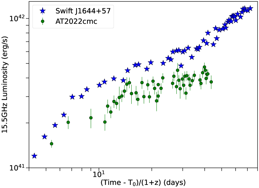
Figure 4: The 15.5 GHz luminosities of Swift J1644 (blue stars) and AT2022cmc (green circles) for the first 100 days in the rest frame of the respective events. The two events show a similar long term evolution for the period in which we have overlap i.e. between 6 and 45 rest frame days. We do not consider the Doppler boosting in calculating the luminosities.

Comparison of the 15.5 GHz luminosities of Swift J1644+57 and AT2022cmc over the first 100 days corrected for their respective redshifts since their respective discovery days (Figure 4). The evolution of both Swift J1644+57 and AT2022cmc show remarkable similarities over the first 40 days in their respective rest frames, where the light curves follow a power law rise of approximately $S_{\nu}\propto t^{0.4}$ (Berger et al., 2012). Unlike in AT2022cmc, Swift J1644+57 shows no statistically significant variability. To infer the same bulk Lorentz factor in the AMI–LA data of Swift J1644+57 as we have for AT2022cmc we would have to observe variability on a timescale of less than one day, a timescale not sampled by the radio follow-up campaigns.

5 Conclusions

Our radio campaign to observe the newly discovered relativistic TDE AT2022cmc has produced high cadence multi-frequency data set spanning the first 100 days post-discovery. The 15.5 GHz light curve shows short timescale variability which corresponds to a very high brightness temperature implying the presence of Doppler boosting and providing a model-independent confirmation of a relativistic outflow. The analysis we have performed here is vital in our long-term understanding, modelling and interpretation of AT2022cmc and other relativistic TDEs. This is the first direct evidence of Doppler beaming in any type of TDE and confirms that such systems are truly relativistic.

Data Availability

All the data used in this paper are available in the online Appendices along with AMI–LA and MeerKAT radio maps and variability consistency checks.

References

- Alexander et al. (2022) Alexander K., et al., 2022, The Astronomer’s Telegram, 15269, 1
- Andreoni et al. (2022a) Andreoni I., et al., 2022a, arXiv e-prints, p. arXiv:2211.16530
- Andreoni et al. (2022b) Andreoni I., et al., 2022b, Transient Name Server AstroNote, 38, 1
- Bannister et al. (2011) Bannister K. W., Murphy T., Gaensler B. M., Hunstead R. W., Chatterjee S., 2011, MNRAS, 412, 634
- Berger et al. (2012) Berger E., Zauderer A., Pooley G. G., Soderberg A. M., Sari R., Brunthaler A., Bietenholz M. F., 2012, ApJ, 748, 36
- Bloom et al. (2011) Bloom J. S., et al., 2011, Science, 333, 203
- Bolton et al. (2006) Bolton R. C., Chandler C. J., Cotter G., Pearson T. J., Pooley G. G., Readhead A. C. S., Riley J. M., Waldram E. M., 2006, MNRAS, 370, 1556
- Bright et al. (2020) Bright J. S., et al., 2020, Nature Astronomy, 4, 697
- Brown et al. (2015) Brown G. C., Levan A. J., Stanway E. R., Tanvir N. R., Cenko S. B., Berger E., Chornock R., Cucchiaria A., 2015, MNRAS, 452, 4297
- Burrows et al. (2011) Burrows D. N., et al., 2011, Nature, 476, 421
- Carotenuto et al. (2022) Carotenuto F., Tetarenko A. J., Corbel S., 2022, MNRAS, 511, 4826
- Cenko et al. (2012) Cenko S. B., et al., 2012, ApJ, 753, 77
- Cenko et al. (2022) Cenko S. B., Andreoni I., Coughlin M., 2022, GRB Coordinates Network, 31729, 1
- Cordes & Lazio (2002) Cordes J. M., Lazio T. J. W., 2002, arXiv e-prints
- Dimple et al. (2022) Dimple et al., 2022, GRB Coordinates Network, 31805, 1
- Dobie et al. (2022) Dobie D., O’Brien A., Zic A., Kaplan D. L., Perley D. A., Ho A. Y. Q., 2022, GRB Coordinates Network, 31665, 1
- Eftekhari et al. (2018) Eftekhari T., Berger E., Zauderer B. A., Margutti R., Alexander K. D., 2018, ApJ, 854, 86
- Fender et al. (2004) Fender R. P., Belloni T. M., Gallo E., 2004, MNRAS, 355, 1105
- Fulton et al. (2022) Fulton M., et al., 2022, Transient Name Server AstroNote, 40, 1
- Ghirlanda et al. (2018) Ghirlanda G., et al., 2018, A&A, 609, A112
- Goodman (1997) Goodman J., 1997, Nature, 2, 449
- Han et al. (2022) Han C., Reynolds M. T., Miller J. M., Gediman B., Hemrattaphan Y., Zak M. K., 2022, The Astronomer’s Telegram, 15349, 1
- Heywood (2020) Heywood I., 2020, oxkat: Semi-automated imaging of MeerKAT observations, Astrophysics Source Code Library, record ascl:2009.003 (ascl:2009.003)
- Hickish et al. (2018) Hickish J., et al., 2018, MNRAS, 475, 5677
- Hovatta et al. (2009) Hovatta T., Valtaoja E., Tornikoski M., Lähteenmäki A., 2009, A&A, 494, 527
- Hunter (2007) Hunter J. D., 2007, Computing in Science Engineering, 9, 90
- Jonas & MeerKAT Team (2016) Jonas J., MeerKAT Team 2016, in MeerKAT Science: On the Pathway to the SKA. p. 1, doi:10.22323/1.277.0001
- Jorstad et al. (2001) Jorstad S. G., Marscher A. P., Mattox J. R., Wehrle A. E., Bloom S. D., Yurchenko A. V., 2001, ApJS, 134, 181
- Jorstad et al. (2005) Jorstad S. G., et al., 2005, AJ, 130, 1418
- Kellermann & Pauliny-Toth (1969) Kellermann K. I., Pauliny-Toth I. I. K., 1969, ApJ, 155, L71
- Lähteenmäki et al. (1999) Lähteenmäki A., Valtaoja E., Wiik K., 1999, ApJ, 511, 112
- Levan et al. (2011) Levan A. J., et al., 2011, Science, 333, 199
- Liodakis et al. (2017) Liodakis I., et al., 2017, MNRAS, 466, 4625
- Longair (2011) Longair M. S., 2011, High Energy Astrophysics, 3rd ed. edn. Cambridge University Press, pp 681–682
- Malzac (2013) Malzac J., 2013, MNRAS, 429, L20
- McMullin et al. (2007) McMullin J. P., Waters B., Schiebel D., Young W., Golap K., 2007, in Shaw R. A., Hill F., Bell D. J., eds, Astronomical Society of the Pacific Conference Series Vol. 376, Astronomical Data Analysis Software and Systems XVI. p. 127
- Mimica et al. (2015) Mimica P., Giannios D., Metzger B. D., Aloy M. A., 2015, MNRAS, 450, 2824
- Mochkovitch et al. (1993) Mochkovitch R., Hernanz M., Isern J., Martin X., 1993, Nature, 361, 236
- Moldon (2021) Moldon J., 2021, eMCP: e-MERLIN CASA pipeline, Astrophysics Source Code Library, record ascl:2109.006 (ascl:2109.006)
- Mooley et al. (2018) Mooley K. P., et al., 2018, Nature, 561, 355
- Mooley et al. (2022) Mooley K. P., Anderson J., Lu W., 2022, Nature, 610, 273
- Mundell et al. (2009) Mundell C. G., Ferruit P., Nagar N., Wilson A. S., 2009, ApJ, 703, 802
- Murphy et al. (2013) Murphy T., et al., 2013, PASA, 30, e006
- Murphy et al. (2017) Murphy T., et al., 2017, MNRAS, 466, 1944
- Ofek et al. (2011) Ofek E. O., Frail D. A., Breslauer B., Kulkarni S. R., Chandra P., Gal-Yam A., Kasliwal M. M., Gehrels N., 2011, ApJ, 740, 65
- Offringa et al. (2014) Offringa A. R., McKinley B., Hurley-Walker et al., 2014, MNRAS, 444, 606
- Pankov et al. (2022) Pankov N., Pozanenko A., Klunko E., Moskvitin A., Maslennikova O. A., Rumyantsev V., Belkin S., IKI FuN G., 2022, GRB Coordinates Network, 31846, 1
- Pasham et al. (2022a) Pasham D. R., et al., 2022a, Nature Astronomy,
- Pasham et al. (2022b) Pasham D., Yao Y., Gendreau K., Perley D., Cenko B., Arzoumanian Z., Ferrara E., 2022b, The Astronomer’s Telegram, 15232, 1
- Pasham et al. (2022c) Pasham D., Gendreau K., Arzoumanian Z., Cenko B., 2022c, GRB Coordinates Network, 31601, 1
- Pearson et al. (1981) Pearson T. J., Unwin S. C., Cohen M. H., Linfield R. P., Readhead A. C. S., Seielstad G. A., Simon R. S., Walker R. C., 1981, Nature, 290, 365
- Perley & Butler (2017) Perley R. A., Butler B. J., 2017, ApJS, 230, 7
- Perley et al. (2022) Perley D., Ho A. Y. Q., Petitpas G., Keating G., 2022, GRB Coordinates Network, 31627, 1
- Perrott et al. (2013) Perrott Y. C., et al., 2013, MNRAS, 429, 3330
- Readhead (1994) Readhead A. C. S., 1994, ApJ, 426, 51
- Rees (1988) Rees M. J., 1988, Nature, 333, 523
- Rees & Meszaros (1994) Rees M. J., Meszaros P., 1994, ApJ, 430, L93
- Rhodes et al. (2020) Rhodes L., et al., 2020, MNRAS, 496, 3326
- Sarbadhicary et al. (2021) Sarbadhicary S. K., et al., 2021, ApJ, 923, 31
- Sari et al. (1999) Sari R., Piran T., Halpern J. P., 1999, ApJ, 519, L17
- Sfaradi et al. (2022) Sfaradi I., Rhodes L., Williams D., Bright J., Horesh A., Fender R., Green D., Titterington D., 2022, GRB Coordinates Network, 31667, 1
- Sincell & Krolik (1994) Sincell M. W., Krolik J. H., 1994, ApJ, 430, 550
- Tanvir et al. (2022) Tanvir N. R., et al., 2022, GRB Coordinates Network, 31602, 1
- Taylor et al. (2004) Taylor G. B., Frail D. A., Berger E., Kulkarni S. R., 2004, ApJ, 609, L1
- Ulrich et al. (1997) Ulrich M.-H., Maraschi L., Urry C. M., 1997, ARAA, 35, 445
- Unwin et al. (1985) Unwin S. C., Cohen M. H., Biretta J. A., Pearson T. J., Seielstad G. A., Walker R. C., Simon R. S., Linfield R. P., 1985, ApJ, 289, 109
- Vaughan et al. (2003) Vaughan S., Edelson R., Warwick R. S., Uttley P., 2003, MNRAS, 345, 1271
- Wagner & Witzel (1995) Wagner S. J., Witzel A., 1995, ARA&A, 33, 163
- Wang et al. (2014) Wang J.-Z., Lei W.-H., Wang D.-X., Zou Y.-C., Zhang B., Gao H., Huang C.-Y., 2014, ApJ, 788, 32
- Yang et al. (2016) Yang J., Paragi Z., van der Horst A. J., Gurvits L. I., Campbell R. M., Giannios D., An T., Komossa S., 2016, MNRAS, 462, L66
- Yao et al. (2022a) Yao Y., Pasham D. R., Gendreau K. C., 2022a, The Astronomer’s Telegram, 15230, 1
- Yao et al. (2022b) Yao Y., Andreoni I., Campana S., Cenko B., 2022b, GRB Coordinates Network, 31641, 1
- Zauderer et al. (2013) Zauderer B. A., Berger E., Margutti R., Pooley G. G., Sari R., Soderberg A. M., Brunthaler A., Bietenholz M. F., 2013, ApJ, 767, 152
- Zou & Piran (2010) Zou Y.-C., Piran T., 2010, MNRAS, 402, 1854
- Zwart et al. (2008) Zwart J. T. L., et al., 2008, MNRAS, 391, 1545
- van der Walt et al. (2011) van der Walt S., Colbert S. C., Varoquaux G., 2011, Computing in Science Engineering, 13, 22