Compression, Generalization and Learning

Abstract

A compression function is a map that slims down an observational set into a subset of reduced size, while preserving its informational content. In multiple applications, the condition that one new observation makes the compressed set change is interpreted that this observation brings in extra information and, in learning theory, this corresponds to misclassification, or misprediction. In this paper, we lay the foundations of a new theory that allows one to keep control on the probability of change of compression (which maps into the statistical “risk” in learning applications). Under suitable conditions, the cardinality of the compressed set is shown to be a consistent estimator of the probability of change of compression (without any upper limit on the size of the compressed set); moreover, unprecedentedly tight finite-sample bounds to evaluate the probability of change of compression are obtained under a generally applicable condition of preference. All results are usable in a fully agnostic setup, i.e., without requiring any a priori knowledge on the probability distribution of the observations. Not only these results offer a valid support to develop trust in observation-driven methodologies, they also play a fundamental role in learning techniques as a tool for hyper-parameter tuning.

Keywords: Compression Schemes, Statistical Risk, Statistical Learning Theory, Scenario Approach

1 Introduction

Compression is an established topic in theoretical learning, and various generalization bounds have been proven for compression schemes.

According to a definition introduced in Littlestone and Warmuth (1986), a compression scheme consists of i. a compression function $\mathsf{c}$, which maps any list of observed examples $S=((x_{1},y_{1}),\ldots,(x_{N},y_{N}))$ ($x_{i}$ is called an “instance” and $y_{i}$ a “label”) into a sub-list $\mathsf{c}(S)$, and ii. a reconstruction function $\rho$, which maps any list of examples $S$ into a classifier $\rho(S)$. An important feature of a classifier is its risk and, in the context of compression schemes, one is interested in the risk associated to the classifier $\rho(\mathsf{c}(S))$. The concept of risk finds a natural definition in statistical learning where one assumes that examples $(x,y)$ are generated according to a random mechanism: the risk of a generic classifier $f$ is then defined as $\mathsf{R}(f)={\mathbb{P}}\{f({\boldsymbol{x}})\neq{\boldsymbol{y}}\}$ (throughout, boldface indicates random quantities). In loose terms, most results in compression schemes establish that low cardinality of the compression implies low risk for the ensuing classifier. A bit more precisely, let ${\boldsymbol{S}}=(({\boldsymbol{x}}_{1},{\boldsymbol{y}}_{1}),\ldots,({\boldsymbol{x}}_{N},{\boldsymbol{y}}_{N}))$ be a list of independent random examples all sharing the same distribution (which coincides with the distribution of $({\boldsymbol{x}},{\boldsymbol{y}})$ in the definition of risk). In the example-consistent framework (i.e., the bound on the risk is only given for lists of examples $S$ for which $\rho(\mathsf{c}(S))$ returns the corresponding label $y_{i}$ for any $x_{i}$ in $S$ – in this case $\rho(\mathsf{c}(S))$ is said to be “consistent” with $S$) and under the assumption that the maximum cardinality of $\mathsf{c}({\boldsymbol{S}})$ is bounded by an integer $d$ ($d$ is called the “size” of the compression scheme), Littlestone and Warmuth (1986) and Floyd and Warmuth (1995) establish results of the type: with high probability $1\!-\!\delta$ with respect to the generation of the list of examples ${\boldsymbol{S}}$, if $\rho(\mathsf{c}({\boldsymbol{S}}))$ is consistent with ${\boldsymbol{S}}$, then the risk of $\mathsf{c}({\boldsymbol{S}})$ is below a known bound that depends on $N$, $d$ and $\delta$ only (in particular, the bound does not depend on the distribution by which examples are generated). Results in this vein have been subsequently extended to the non-consistent framework and to compression schemes with unbounded size, in which context the best known results are given in Graepel et al. (2005).

In a series of recent papers, compression schemes have been studied under a stability condition, a notion that is natural in many contexts and that has its roots in Vapnik and Chervonenkis (1974). For the example-consistent framework and compression schemes with bounded size, Bousquet et al. (2020) succeeded in removing a $\log(N)$ term in the expression of the bound for the risk as compared to the formulation given in the above referenced papers; when applied to Support Vector Machines, this result resolves a long-standing issue that was posed in – and remained open since – Vapnik and Chervonenkis (1974). Later, the scope of Bousquet et al. (2020) has been significantly broadened by Hanneke and Kontorovich (2021), where the non-consistent framework with no upper bounds on the size of the compression scheme has been considered. Since the stable case is most relevant to the present paper, we shall come back to these latter contributions with a more detailed discussion and comparison at the end of Section 3.

In the present paper, we make a paradigm shift: since we are interested in compression as a general tool applicable across various domains, we are well-advised to adopt a “purist” approach in which compression functions are studied in isolation (without a reconstruction function). Our essential goal is to study how the probability of change of compression relates to the size of the compressed set. The corresponding results can be applied to supervised learning, unsupervised learning and, in addition, to any other contexts where compression functions are in use. Our findings are summarized at the end of this section, we start with introducing the formal elements of the problem.

1.1 Mathematical setup and notation

Examples $z$ are elements from a set $\mathcal{Z}$ (for instance, in supervised learning $z$ are pairs $(x,y)$). The compression functions we study are permutation invariant. Correspondingly, given any $n=0,1,2,\ldots$ and a list of examples $(z_{1},\dots,z_{n})$, we introduce the associated multiset written as $\mathsf{ms}(z_{1},\dots,z_{n})$, where the operator “$\mathsf{ms}$” removes the ordering in the list, while maintaining repetitions. The set operations $\cup,\cap,\setminus$ (union, intersection, and set difference) are easily extended to multisets using the notion of multiplicity function $\mu_{U}$ for a multiset $U$, which counts how many times each element of $\mathcal{Z}$ occurs in $U$. Then, $\mu_{U\cup U^{\prime}}(z)=\mu_{U}(z)+\mu_{U^{\prime}}(z)$, $\mu_{U\cap U^{\prime}}(z)=\min\big{\{}\mu_{U}(z),\mu_{U^{\prime}}(z)\big{\}}$, and $\mu_{U\setminus U^{\prime}}(z)=\max\big{\{}0,\mu_{U}(z)-\mu_{U^{\prime}}(z)\big{\}}$. Moreover, $U\subseteq U^{\prime}$ means that $\mu_{U}(z)\leq\mu_{U^{\prime}}(z)$ for all $z$, and $|U|$ stands for the cardinality of a multiset where each example is counted as many times as is its multiplicity. Throughout this paper, multisets have always finite cardinality and, any time a multiset is introduced, it is tacitly assumed that it has finitely many elements. A compression function $\mathsf{c}$ is a map from any multiset of examples $U$ to a sub-multiset: $\mathsf{c}(U)\subseteq U$. We write $\mathsf{c}(z_{1},\ldots,z_{n})$ as a shortcut for $\mathsf{c}(\mathsf{ms}(z_{1},\ldots,z_{n}))$. Also, given a multiset $U$ and one more example $z$, $\mathsf{c}(U,z)$ stands for $\mathsf{c}(U\cup\mathsf{ms}(z))$. Similar notations apply to other maps having a multiset as argument. Throughout, an example is modeled as a realization of a random element defined over a probability space $(\Omega,\mathcal{F},{\mathbb{P}})$; moreover, a list of $n$ examples is the realization of the first $n$ elements of an independent and identically distributed (i.i.d.) sequence ${\boldsymbol{z}}_{1},{\boldsymbol{z}}_{2},\ldots$. A training set is a multiset generated from a list of observed examples. When dealing with problems in machine learning, a learning algorithm $\mathcal{A}$ is a map from training sets to a hypothesis $h$ in a set $\mathcal{H}$ (in supervised binary classification, $h$ is a concept; in supervised learning with continuous label, $h$ is a predictor; in unsupervised learning, $h$ can, e.g., be a collection of clusters; etc.). According to the above notation, we write $\mathcal{A}(z_{1},\dots,z_{N})$ to denote the hypothesis generated by $\mathcal{A}$ when the input is the training set $\mathsf{ms}(z_{1},\dots,z_{N})$. We use a $\{0,1\}$-valued function $\ell(h,z)$ to indicate whether or not a hypothesis $h$ is appropriate for an example $z$: $\ell(h,z)=0$ signifies that $h$ is appropriate for $z$, while $\ell(h,z)=1$ corresponds to inappropriateness (for instance, in supervised classification, $\ell(h,z)=\mathbbm{1}_{h(x)\neq y}$, where $\mathbbm{1}$ is the indicator function). The statistical risk of $h$ is $\mathsf{R}(h)={\mathbb{P}}\{\ell(h,{\boldsymbol{z}})=1\}$, where ${\boldsymbol{z}}$ is a random element distributed as each ${\boldsymbol{z}}_{i}$.

1.2 Main contributions

The contributions of this paper are summarized in the following three points.

(i) Under the property of preference, Theorem 4 establishes a new bound to the probability of change of compression as a function of the cardinality of the compressed multiset. For a finite size of the training set, the bound is informative and useful in applications (see Figure 2). When the size of the training set $N$ tends to infinity, the bound tends to the ratio $k/N$ (where $k$ is the cardinality of the compressed multiset), uniformly in $k\in\{0,1,\ldots,N\}$ (the fact that the range for $k$ arrives at $N$ means that the compressed multiset has no upper limits other than the size of the training set itself), see Proposition 8. No lower bounds to the probability of change of compression are possible under the sole preference property. Under an additional non-associativity property and a condition of non-concentrated probabilistic mass, Theorem 7 establishes a lower bound (see Figure 3). This lower bound also converges to $k/N$ uniformly in $k\in\{0,1,\ldots,N\}$. Hence, under the assumptions of Theorem 7, the probability of change of compression is in sandwich between two bounds that merge one on top of the other as $N\to\infty$ (see Proposition 8). This entails that the cardinality of the compressed multiset is a highly informative statistics to evaluate the probability of change of compression.

(ii) In Section 3, the results in (i) are put at work to study classical compression schemes in the presence of a reconstruction function. It is shown that a preferent compression scheme augmented with the examples that are misclassified preserves the preference property. From this, one finds that the risk can be evaluated without resorting to an incremental approach (as it was customary in previous contributions) in which the empirical risk is incremented with an estimate of the mismatch between empirical and actual risk. The resultant evaluations of the risk, established in Theorem 17, are unprecedentedly sharp. Under the additional conditions of non-associativity and of non-concentrated mass, if certain coherence properties hold, then one obtains bounds on the risk that are valid both from above and from below, which provides a statistically consistent evaluation of the risk. Empirical demonstrations complement the theoretical study and show that the bounds cover tightly the actual stochastic dispersion of the risk.

(iii) As examples of application, the achievements in point (ii) are applied in Section 4 to various support vector methods, including the Support Vector Machine (SVM) and the Support Vector Regression (SVR), and to the Guaranteed Error Machine (GEM). This study shows that, in various learning contexts, one can identify statistics of the data from which consistent estimates of the risk can be obtained without resorting to validation or testing.

1.3 Relation with previous contributions and a more general perspective on this work

The scientific background in which this work has matured lies in some fifteen years of work by its authors in the field of data-driven optimization. In a group of papers, whose forefathers are Calafiore and Campi (2005, 2006); Campi and Garatti (2008) and that include Campi and Garatti (2011); Campi and Carè (2013); Carè et al. (2015); Campi et al. (2018); Garatti et al. (2019, 2023); Garatti and Campi (2023), they laid with co-authors the foundations of the so-called “scenario approach”, a vast body of methods and algorithms to obtain data-driven, theoretically-certified, solutions to uncertain optimization problems. The scenario approach has spurred quite a bit of work also done by others, as witnessed by a large number of theoretical contributions, of which we here only mention the most significant ones: Welsh and Rojas (2009); Welsh and Kong (2011); Pagnoncelli et al. (2012); Schildbach et al. (2013, 2014); Margellos et al. (2014, 2015); Zhang et al. (2015); Esfahani et al. (2015); Crespo et al. (2015); Grammatico et al. (2016); Crespo et al. (2016); Lacerda and Crespo (2017); Margellos et al. (2018); Crespo et al. (2019); Falsone et al. (2019). Recently, the studies on scenario optimization have culminated in the works Campi and Garatti (2018); Garatti and Campi (2022), which are conceptually linked to the present contribution by the fact that the generalization properties of the solution are evaluated from an observable called “complexity” (complexity parallels the size of the compressed multiset of this paper). As compared with all this previous literature, the present contribution introduces two major elements of novelty:

(a) compression takes center stage, beyond any contextualization. By this purist approach, we aim to lay the groundwork for a new theory of wide applicability, to machine learning in primis, but also across the other multiple data science fields in which compression finds application;

(b) by a novel, powerful, theoretical apparatus, this paper establishes bounds on the risk that fare beyond the domain of previous contributions; in particular, they allow one to drop any condition of non-degeneracy, which was a standing and limiting assumption in previous works, e.g., Campi and Garatti (2018); Garatti and Campi (2022).

We hope that the findings presented in this paper will open a new era of exploration and discovery in an important subarea of data-driven methods that is centered around the notion of compression. As previously mentioned, we here already consider support vector methods and improve the results in Campi and Garatti (2021) by eliminating all assumptions on the distribution of the examples for the problem of obtaining upper bounds on the risk. We also study a generalized version of the so-called Guaranteed Error Machine, which was introduced in Campi (2010) under a limiting condition on the complexity of the classifier. Beyond the applications discussed in this paper, we expect that our results will prove useful in various fields where the scenario approach is applicable (including robust optimization, with its multiform applications to diverse contexts). We feel like to also mention that the authors of this paper are at present actively exploring a wide range of example-driven computer science algorithms in which the application of the compression theory of this paper is made possible through an importance procedure for example selection, even in cases where the original algorithm lacks any compression (see Paccagnan et al. (2023) for a study in the context of machine learning). For a broader discussion on the increasing importance of establishing well-founded risk theories for data-driven decision processes, particularly in today’s time in which the use of data is becoming pervasive, the reader is referred to the recent position paper Campi et al. (2021).

1.4 Structure of the paper

The main results on compression schemes are presented in a unified treatment in the next Section 2, which also includes a discussion on the asymptotic behavior of the bounds. Section 3 presents a rapprochement with classical compression schemes in statistical learning that incorporate a reconstruction function, along with some other more general results useful for machine learning problems. Specific machine learning schemes are considered in Section 4. The proofs of the main results are deferred till Section 5.

2 New generalization results for compression schemes

Our interest lies in quantifying the probability with which a change of compression occurs. As it was mentioned in the introduction, and it will be further explored in Section 4, this probability has important implications in relation to learning schemes. We start with a formal definition of probability of change of compression.

Definition 1 (probability of change of compression)

The probability of change of compression is defined as

$$\phi({\boldsymbol{z}}_{1},\dots,{\boldsymbol{z}}_{n})={\mathbb{P}}\{\mathsf{c}(\mathsf{c}({\boldsymbol{z}}_{1},\ldots,{\boldsymbol{z}}_{n}),{\boldsymbol{z}}_{n+1})\neq\mathsf{c}({\boldsymbol{z}}_{1},\ldots,{\boldsymbol{z}}_{n})|{\boldsymbol{z}}_{1},\ldots,{\boldsymbol{z}}_{n}\}.$$

$\star$

On the right-hand side a new element ${\boldsymbol{z}}_{n+1}$ is added to the compression of $\mathsf{ms}({\boldsymbol{z}}_{1},\dots,{\boldsymbol{z}}_{n})$  and it is tested whether this makes the compression change. This gives an event, and our interest lies in the probability of this event. However, in view of its use in applications, what matters is not the probability tout court, rather, we take a more fine-grained standpoint by conditioning on ${\boldsymbol{z}}_{1},\ldots,{\boldsymbol{z}}_{n}$, so as to capture the variability of the probability of change of compression as determined by the examples. This makes $\phi({\boldsymbol{z}}_{1},\dots,{\boldsymbol{z}}_{n})$ into a random variable. In what follows, we shall often use the symbol ${\boldsymbol{\phi}}_{n}$ as a shorthand for the random variable $\phi({\boldsymbol{z}}_{1},\dots,{\boldsymbol{z}}_{n})$.

Before delving into the mathematical developments, we are well-advised to digress a moment to discuss the nature of the results we mean to reach. Let $N$ be the size of the multiset at hand, the one of which we want to study the probability of change of compression. ${\boldsymbol{\phi}}_{N}$ has a probability distribution of its own. Arguably, this distribution may vary significantly with the distribution by which the $z_{i}$’s are generated. This fact has an important implication: any result that describes the distribution of ${\boldsymbol{\phi}}_{N}$ without referring to some prior knowledge on the distribution of the ${\boldsymbol{z}}_{i}$’s is bound to stay on the conservative side and is therefore poorly informative. While this may seem to set fundamental limitations to obtaining distribution-free results on ${\boldsymbol{\phi}}_{N}$ (i.e., results valid without any a priori knowledge on the distribution of the ${\boldsymbol{z}}_{i}$’s), nevertheless it turns out that this conclusion is hasty and incorrect: indeed, one can instead move along a different path and take a bi-variate standpoint, as next explained. Let $|\mathsf{c}({\boldsymbol{z}}_{1},\ldots,{\boldsymbol{z}}_{N})|$ be the cardinality of the compressed multiset $\mathsf{c}({\boldsymbol{z}}_{1},\ldots,{\boldsymbol{z}}_{N})$. We consider the pair $(|\mathsf{c}({\boldsymbol{z}}_{1},\ldots,{\boldsymbol{z}}_{N})|,{\boldsymbol{\phi}}_{N})$ and identify conditions of general interest under which its bi-variate distribution concentrates in a slender, lenticular-shaped, region (see Figure 3). The implications are quite notable: within the lenticular-shaped region, the distribution of $(|\mathsf{c}({\boldsymbol{z}}_{1},\ldots,{\boldsymbol{z}}_{N})|,{\boldsymbol{\phi}}_{N})$ does exhibit a strong variability depending on the problem (which also translates into the variability of the marginal distribution of ${\boldsymbol{\phi}}_{N}$). However, given the realization of ${\boldsymbol{z}}_{1},\ldots,{\boldsymbol{z}}_{N}$ at hand, one can compute the value of $|\mathsf{c}({\boldsymbol{z}}_{1},\ldots,{\boldsymbol{z}}_{N})|$ and intersect the vertical line corresponding to this value with the lenticular-shaped region to obtain an interval for the probability of the change of compression. The so-formulated evaluation is tight and informative even for small values of $N$ and offers an useful assessment tool for applications. Importantly, the corresponding theory retains the characteristic of being distribution-free. This finding is stated below as Theorem 7 and it holds under two properties called preference (Property 2) and non-associativity (Property 5), besides a condition that rules out concentrated masses (Property 6). Interestingly, under the sole preference property, only the lower bound of the lenticular-shaped region is lost while the upper bound maintains its validity (Theorem 4), which provides a result broadly applicable to evaluate an upper limit on the probability of change of compression as a function of the cardinality of the compressed multiset.

Moving towards the mathematical results, we first formalize the concept of preference.

Property 2 (preference)

For any multisets $U$ and $V$ such that $V\subseteq U$, if $V\neq\mathsf{c}(U)$, then $V\neq\mathsf{c}(U,z)$ for all $z\in\mathcal{Z}$. $\star$

Hence, if a sub-multiset is not chosen as the compressed multiset, then it cannot become the compressed multiset at a later stage after augmenting the multiset with a new example.

The following lemma provides a useful reformulation of the preference property.

Lemma 3

A compression function $\mathsf{c}$ satisfies the preference property if and only if $\mathsf{c}(V)=\mathsf{c}(U)$ for all multisets $U,V$ such that $\mathsf{c}(U)\subseteq V\subseteq U$. $\star$

Proof  Assume $\mathsf{c}$ satisfies the preference property and let $z_{1},\ldots,z_{n}$ be the elements in $U\setminus V$ where $U$ and $V$ are multisets such that $\mathsf{c}(U)\subseteq V\subseteq U$. Let $S_{0}=V$ and $S_{i}=S_{i-1}\cup\mathsf{ms}(z_{i})$ for $i=1,\ldots,n$ so that $S_{n}=U$. Now suppose that $\mathsf{c}(V)\neq\mathsf{c}(U)$. Since $\mathsf{c}(S_{0})=\mathsf{c}(V)$ and $\mathsf{c}(S_{n})=\mathsf{c}(U)$, then it must be that $\mathsf{c}(S_{i-1})\neq\mathsf{c}(U)$ and $\mathsf{c}(S_{i-1},z_{i})=\mathsf{c}(U)$ for some $i\in\{1,\ldots,n\}$. However, since $\mathsf{c}(U)\subseteq S_{i-1}$, this contradicts the assumption that $\mathsf{c}$ satisfies the preference property.
For the other direction, assume that the preference property does not hold. Then, we can find $U,V,z$ such that $V\subseteq U$ and $\mathsf{c}(U)\neq V=\mathsf{c}(U,z)$. This implies $\mathsf{c}(U,z)\subseteq U\subseteq U\cup\mathsf{ms}(z)$ and $\mathsf{c}(U)\neq\mathsf{c}(U,z)$, contradicting the statement that $\mathsf{c}(V^{\prime})=\mathsf{c}(U^{\prime})$ for all multisets $U^{\prime},V^{\prime}$ such that $\mathsf{c}(U^{\prime})\subseteq V^{\prime}\subseteq U^{\prime}$.  
An immediate consequence of Lemma 3 is that $\mathsf{c}\big{(}\mathsf{c}(U)\big{)}=\mathsf{c}(U)$ whenever $c$ satisfies the preference property.

The statement of our first theorem is better enunciated by introducing the following functions $\Psi_{k,\delta}:(0,1)\to\mathbb{R}$, which are indexed by $k=0,1,\ldots,N-1$ and by the confidence parameter $\delta\in(0,1)$:

$$\Psi_{k,\delta}(\alpha)=\frac{\delta}{N}\sum_{m=k}^{N-1}\frac{\binom{m}{k}}{\binom{N}{k}}(1-\alpha)^{-(N-m)}~{}.$$

For any $k$ and any $\delta$, the equation $\Psi_{k,\delta}(\alpha)=1$ admits one and only one solution in $(0,1)$. Indeed, $\Psi_{k,\delta}(\alpha)$ is strictly increasing, continuous, and $\Psi_{k,\delta}(\alpha)\leq\delta<1$ when $\alpha\to 0$, while it grows to $+\infty$ when $\alpha\to 1$ (see Figure 1(a)).

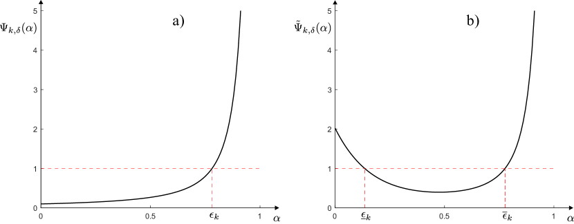
Figure 1: (a) Function $\Psi_{k,\delta}(\alpha)$: it starts below $\delta$ when $\alpha\to 0$ and tends to $+\infty$ when $\alpha\to 1$; (b) Function $\tilde{\Psi}_{k,\delta}(\alpha)$: it tends to $+\infty$ as $\alpha\to 1$ or $\alpha\to-\infty$ and takes a value below $1$ in a point in $(-\infty,1)$.

Define

$$\varepsilon_{k}=\begin{cases}\mbox{solution to }\Psi_{k,\delta}(\alpha)=1,&k=0,1,\ldots,N-1;\\ 1,&k=N.\end{cases}$$ (1)

Theorem 4

Assume the preference Property 2. For any $\delta\in(0,1)$, it holds that

$${\mathbb{P}}\{{\boldsymbol{\phi}}_{N}>\varepsilon_{\boldsymbol{k}}\}\leq\delta,$$ (2)

where $\varepsilon_{\boldsymbol{k}}$ is the random variable obtained by the composition of ${\boldsymbol{k}}:=|\mathsf{c}({\boldsymbol{z}}_{1},\ldots,{\boldsymbol{z}}_{N})|$ (the cardinality of the multiset $\mathsf{c}({\boldsymbol{z}}_{1},\ldots,{\boldsymbol{z}}_{N})$) with the function $\varepsilon_{k}$ given in (1) (in other words, it is $\varepsilon_{k}$ evaluated at the random value ${\boldsymbol{k}}$). $\star$

Proof  The proof of Theorem 4 is given in Section 5.2.  
In the theorem, parameter $\delta$ is called the “confidence parameter” and it is normally selected to a very small value, say $10^{-5}$ or $10^{-6}$. The theorem claims that ${\boldsymbol{\phi}}_{N}$, the probability of change of compression, is upper-bounded, with high confidence $1-\delta$, by $\varepsilon_{\boldsymbol{k}}$, which is a known, deterministic, function $\varepsilon_{k}$ evaluated in correspondence of the cardinality ${\boldsymbol{k}}$ of the compressed multiset. Figure 2 visualizes function $\varepsilon_{k}$ for $N=2000$ and various values of $\delta$.

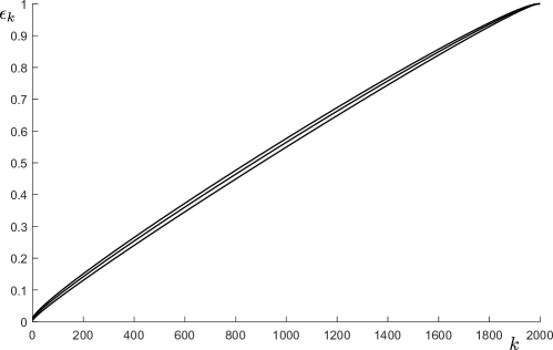
Figure 2: Curve $\varepsilon_{k}$ against the value of $k$ for $N=2000$ and various values of $\delta$ ($10^{-3}$, $10^{-6}$, and $10^{-9}$). As established in Theorem 4, for preferent compression functions this curve sets an upper bound (valid with confidence $1-\delta$) on the probability of change of compression as a function of the cardinality $k$ of the compressed multiset.

In machine learning applications, the interest of Theorem 4 stems from the fact that a change of compression occurs when an example is misclassified, or mispredicted. Hence, the theorem allows one to upper-bound the probability of misclassification, or misprediction, by using an observable, the cardinality of the compressed multiset. Importantly, the evaluation holds independently of the distribution of the ${\boldsymbol{z}}_{i}$’s, hence the user can apply the result without positing any, possibly hazardous, conjecture on how data are generated. An ample space to the use of Theorem 4 in machine learning problems is given in Sections 3 and 4.

Lower and upper bounds on ${\boldsymbol{\phi}}_{N}$ are established under additional conditions, the non-associativity Property 5 and the Property 6 of non-concentrated mass, as described in the following.

Property 5 (non-associativity)

For any $n\geq 0$ and $p\geq 1$,

$${\mathbb{P}}\big{(}E_{1}\setminus E_{2}\big{)}=0,$$

where

$$E_{1}=\{\mathsf{c}({\boldsymbol{z}}_{1},\ldots,{\boldsymbol{z}}_{n},{\boldsymbol{z}}_{n+i})=\mathsf{c}({\boldsymbol{z}}_{1},\ldots,{\boldsymbol{z}}_{n}),\;i=1,\dots,p\},$$

$$E_{2}=\{\mathsf{c}({\boldsymbol{z}}_{1},\ldots,{\boldsymbol{z}}_{n},{\boldsymbol{z}}_{n+1},\ldots,{\boldsymbol{z}}_{n+p})=\mathsf{c}({\boldsymbol{z}}_{1},\ldots,{\boldsymbol{z}}_{n})\}.$$

$\star$

In words, the non-associativity property can be phrased as follows: if the compression does not change adding elements one at a time, then it does non change when they are added altogether, with the possible exception of an event whose probability is zero. The reader may have noticed that Property 5 is given in probability unlike the preference Property 2, which was required to hold for any choice of the examples. The reason is that requiring the validity of the non-associativity property for all examples can be restrictive in some applications.

Property 6 (non-concentrated mass)

$${\mathbb{P}}\{{\boldsymbol{z}}_{i}=z\}=0,\;\forall z\in\mathcal{Z}.$$

$\star$

The property of non-concentrated mass simply requires that any $z$ can only be drawn with probability zero and, hence, it excludes with probability $1$ that the same $z$ occurs twice or more times in a training set.

Theorem 7 is stated by means of the following functions $\tilde{\Psi}_{k,\delta}:(-\infty,1)\to\mathbb{R}$ indexed by $k=0,1,\ldots,N$ and by the confidence parameter $\delta\in(0,1)$:

for $k=0,\ldots,N-1$, let

$$\tilde{\Psi}_{k,\delta}(\alpha)=\frac{\delta}{2N}\sum_{m=k}^{N-1}\frac{{m\choose k}}{{N\choose k}}(1-\alpha)^{-(N-m)}+\frac{\delta}{6N}\sum_{m=N+1}^{4N}\frac{{m\choose k}}{{N\choose k}}(1-\alpha)^{m-N},$$ (3)

while, for $k=N$, let

$$\tilde{\Psi}_{N,\delta}(\alpha)=\frac{\delta}{6N}\sum_{m=N+1}^{4N}{m\choose N}(1-\alpha)^{m-N}.$$

In Appendix A it is shown that, for $k=0,1,\ldots,N-1$, equation $\tilde{\Psi}_{k,\delta}(\alpha)=1$ admits two and only two solutions in $(-\infty,1)$, say $\underline{\alpha}_{k}$ and $\overline{\alpha}_{k}$, with $\underline{\alpha}_{k}<\frac{k}{N}<\overline{\alpha}_{k}$ (see Figure 1(b) for a graphical visualization of $\tilde{\Psi}_{k,\delta}(\alpha)$, $k<N$). Instead, equation $\tilde{\Psi}_{N,\delta}(\alpha)=1$ admits only one solution in $(-\infty,1)$, which is denoted by $\underline{\alpha}_{N}$ (this is easy to verify because $\tilde{\Psi}_{N,\delta}(\alpha)$ is strictly decreasing and it tends to $0$ as $\alpha\to 1$ while it grows to $+\infty$ as $\alpha\to-\infty$). Define

$$\underline{\varepsilon}_{k}=\max\{0,\underline{\alpha}_{k}\},\quad k=0,1,\ldots,N,$$ (4)

and

$$\overline{\varepsilon}_{k}=\begin{cases}\overline{\alpha}_{k},&k=0,1,\ldots,N-1;\\ 1,&k=N.\end{cases}$$ (5)

Theorem 7

Assume the preference Property 2, the non-associativity Property 5 and the non-concentrated mass Property 6. For any $\delta\in(0,1)$, it holds that

$${\mathbb{P}}\{\underline{\varepsilon}_{\boldsymbol{k}}\leq{\boldsymbol{\phi}}_{N}\leq\overline{\varepsilon}_{\boldsymbol{k}}\}\geq 1-\delta,$$ (6)

where $\underline{\varepsilon}_{\boldsymbol{k}}$ is the random variable obtained by the composition of ${\boldsymbol{k}}:=|\mathsf{c}({\boldsymbol{z}}_{1},\ldots,{\boldsymbol{z}}_{N})|$ with the function $\underline{\varepsilon}_{k}$ given in (4) and $\overline{\varepsilon}_{\boldsymbol{k}}$ is the random variable obtained by the composition of ${\boldsymbol{k}}$ with the function $\overline{\varepsilon}_{k}$ given in (5). $\star$

Proof  The proof of Theorem 7 is given in Section 5.3.  

With the additional properties of non-associativity and non-concentrated mass, Theorem 7 assigns upper and lower bounds for the change of compression, as visualized in Figure 3.

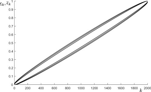
Figure 3: Region delimited by $\underline{\varepsilon}_{k}$ and $\overline{\varepsilon}_{k}$ for $N=2000$ and various values of $\delta$ ($10^{-3}$, $10^{-6}$, and $10^{-9}$). Under the assumptions of Theorem 7, this region contains with confidence $1-\delta$ the probability of change of compression as a function of the cardinality of the compressed multiset.

Strictly speaking, these additional requirements do depend on the underlying probability by which examples are generated and, hence, they cannot be labeled as being “distribution-free”. Nonetheless, in various situations, Theorem 7 becomes applicable under a very limited knowledge on the distribution of the ${\boldsymbol{z}}_{i}$’s, and we shall see examples of this in Section 4. We also note that dropping the assumption of non-concentrated mass makes Theorem 7 false, as shown in the following counterexample. Suppose that one single element $\bar{z}$ has probability $1$ to be selected (so that the non-concentrated mass property is violated), fix any integer $M$ (for example $M=100$) and consider the compression function that returns the initial multiset any time this multiset includes the element $\bar{z}$ less than $M$ times, while it trims the number of elements $\bar{z}$ to $M$ when $\bar{z}$ appears more than $M$ times in the initial multiset. It is easily seen that the preference and non-associativity properties hold. On the other hand, for $N\geq M$ the probability of change of compression is zero with probability $1$, so that no meaningful lower bounds can be assigned in this example.

2.1 Asymptotic behavior of $\varepsilon_{k}$ and $\underline{\varepsilon}_{k}$, $\overline{\varepsilon}_{k}$

The purpose of this section is to establish explicit lower and upper bounds on $\varepsilon_{k}$ and $\overline{\varepsilon}_{k}$, $\underline{\varepsilon}_{k}$ able to reveal the dependencies of these quantities on $k$, $N$, and $\delta$, and also to pinpoint convergence properties as $N$ tends to infinity. The main result is in Proposition 8, followed by some comments. We advise the reader that the explicit bounds in Proposition 8 are in use to clarify various dependencies, but they are not meant for practical computation since they lead to conservative results if used in place of the numerical procedures given in Appendix B.

Proposition 8

$$\overline{\varepsilon}_{k} \;\leq\;\frac{k}{N}+2\frac{\sqrt{k+1}}{N}\left(\sqrt{\ln(k+1)}+4\right)+2\frac{\sqrt{k+1}\sqrt{\ln\frac{1}{\delta}}}{N}+\frac{\ln\frac{1}{\delta}}{N}$$ (7)

$$\underline{\varepsilon}_{k} \;\geq\;\frac{k}{N}-3\frac{\sqrt{k+1}}{N}\left(\sqrt{\ln(k+1)}+2\right)-3\frac{\sqrt{k+1}\sqrt{\ln\frac{1}{\delta}}}{N}.$$ (8)

Moreover, it holds that

$$\frac{k}{N}\leq\varepsilon_{k} \;\leq\;\overline{\varepsilon}_{k}$$

Proof  The proof of Proposition 8 is given in Section 5.4.  
In both (7) and (8), the dependence on $\delta$ is inversely logarithmic, which shows that “confidence is cheap”: very small values of $\delta$ can be enforced without significantly affecting the results and, thereby, the width of the interval $[\underline{\varepsilon}_{k},\overline{\varepsilon}_{k}]$ (see again Figure 3). For any fixed $k$, we see that $\varepsilon_{k}$ and $\overline{\varepsilon}_{k}$, $\underline{\varepsilon}_{k}$ tend to $k/N$ as $O(1/N)$, while for $k$ that grows at the same rate as $N$ (say $k/N$ = constant) $\varepsilon_{k}$ and $\overline{\varepsilon}_{k}$, $\underline{\varepsilon}_{k}$ converge towards $k/N$ as $O(\sqrt{\ln(N)}/\sqrt{N})$. This is just marginally slower than the convergence rate for the law of large numbers, as given by the central limit theorem.

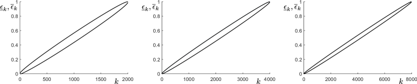
Figure 4: Graph of $\overline{\varepsilon}_{k}$, and $\underline{\varepsilon}_{k}$ as functions of $k$ for $\delta=10^{-6}$ and $N=2000$, $4000$, and $8000$.

The evolution of $\overline{\varepsilon}_{k}$, $\underline{\varepsilon}_{k}$ as $N$ grows can be seen in Figure 4.

Reading the results of this section in the light of Theorem 4, one concludes that, for all compression functions satisfying the preference Property 2, the bi-variate distribution of ${\boldsymbol{k}}=|\mathsf{c}({\boldsymbol{z}}_{1},\ldots,{\boldsymbol{z}}_{N})|$ and ${\boldsymbol{\phi}}_{N}$ all lies below the line $k/N$ plus an offset whose size goes to zero as $O(\sqrt{\ln(N)}/\sqrt{N})$ with the exception of a slim tail whose probabilistic mass is no more than $\delta$. If, additionally, Properties 5 and 6 hold, Theorem 7 shows that the bi-variate distribution of ${\boldsymbol{k}}=|\mathsf{c}({\boldsymbol{z}}_{1},\ldots,{\boldsymbol{z}}_{N})|$ and ${\boldsymbol{\phi}}_{N}$ all lies in a strip around $k/N$ whose size goes to zero as $O(\sqrt{\ln(N)}/\sqrt{N})$ but a slim tail. In this latter case, Theorem 7 also carries the very important implication that the ratio ${\boldsymbol{k}}/N$ is a strongly consistent estimator of ${\boldsymbol{\phi}}_{N}$ irrespective of the problem at hand (it can be proven that Theorem 7 and Proposition 8 together imply that $|{\boldsymbol{k}}/N-{\boldsymbol{\phi}}_{N}|$ converges to zero both in the mean square sense and almost surely).

3 Compression schemes for machine learning

The aim of this section is to connect the theory of Section 2 to that of statistical risk in learning algorithms. Our findings will be compared with existing results at the end of this section. Refer to Section 1.1 for the mathematical setup and notation.

Given a learning algorithm $\mathcal{A}$, suppose that there exists a compression function $\mathsf{c}$ that ties in with the loss function $\ell$ according to the following property.

Property 9 (coherence – part I)

For any $n\geq 0$ and any choice of $z_{1},\ldots,z_{n},z_{n+1}\in\mathcal{Z}$, if $\ell\big{(}\mathcal{A}(z_{1},\ldots,z_{n}),z_{n+1}\big{)}=1$, then $\mathsf{c}\big{(}\mathsf{c}(z_{1},\ldots,z_{n}),z_{n+1}\big{)}\neq\mathsf{c}(z_{1},\ldots,z_{n})$. $\star$

Under Property 9, $\mathsf{R}(\mathcal{A}({\boldsymbol{z}}_{1},\ldots,{\boldsymbol{z}}_{N}))\leq{\boldsymbol{\phi}}_{N}$ holds with probability $1$, and Theorem 4 can be used to bound the risk of the hypothesis returned by the learning algorithm, as specified in the following theorem.

Theorem 10

Given a learning algorithm $\mathcal{A}$, suppose that there exists a compression function $\mathsf{c}$ that satisfies the coherence – part I Property 9. Assume the preference Property 2. For any $\delta\in(0,1)$, it holds that

$${\mathbb{P}}\Big{\{}\mathsf{R}\big{(}\mathcal{A}({\boldsymbol{z}}_{1},\ldots,{\boldsymbol{z}}_{N})\big{)}>\varepsilon_{\boldsymbol{k}}\Big{\}}\leq\delta,$$

where ${\boldsymbol{k}}=|\mathsf{c}({\boldsymbol{z}}_{1},\ldots,{\boldsymbol{z}}_{N})|$ and $\varepsilon_{k}$ is given in (1). $\star$

We next provide a sufficient condition for Property 9 to hold for the case in which the learning algorithm can be reconstructed from the compressed multiset.

Definition 11 (reconstruction function)

Given a learning algorithm $\mathcal{A}$ and a compression function $\mathsf{c}$, a reconstruction function $\rho$ is a map from multisets to hypotheses such that $\rho\big{(}\mathsf{c}(z_{1},\ldots,z_{n})\big{)}=\mathcal{A}(z_{1},\ldots,z_{n})$ for any multiset $\mathsf{ms}(z_{1},\dots,z_{n})$. $\star$

We also need the following property, which requires that the examples in the training set for which the hypothesis chosen by the learning algorithm $\mathcal{A}$ is inappropriate are included in the compressed multiset.

Property 12 (inclusion)

For any multiset $\mathsf{ms}(z_{1},\ldots,z_{n})$ and for any $i=1,2,\ldots,n$, if $\ell\big{(}\mathcal{A}(z_{1},\ldots,z_{n}),z_{i}\big{)}=1$, then $z_{i}$ appears in $\mathsf{c}(z_{1},\ldots,z_{n})$ the same number of times as it appears in $\mathsf{ms}(z_{1},\ldots,z_{n})$. $\star$

The following lemma shows that inclusion implies coherence – part I whenever $\mathcal{A}$ admits a reconstruction function for the given $\mathsf{c}$.

Lemma 13

Given a learning algorithm $\mathcal{A}$ and a compression function $\mathsf{c}$ satisfying the inclusion Property 12, if there exists a reconstruction function for $(\mathcal{A},\mathsf{c})$, then the coherence – part I Property 9 holds. $\star$

Proof  We prove that, under inclusion and existence of a reconstruction function, absence of change of compression is necessarily associated to appropriateness (contrapositive of coherence – part I Property 9).

Let $U:=\mathsf{ms}(z_{1},\ldots,z_{n})$ and suppose that for a new $z_{n+1}$ the compression does not change, i.e.,

$$\mathsf{c}\big{(}\mathsf{c}(U),z_{n+1}\big{)}=\mathsf{c}(U).$$ (9)

Applying $\rho$ to both sides of (9) and using the definition of reconstruction function gives

$$\mathcal{A}\big{(}\mathsf{c}(U),z_{n+1}\big{)}=\mathcal{A}(U).$$ (10)

On the other hand, (9) implies that $z_{n+1}$ appears in $\mathsf{c}\big{(}\mathsf{c}(U),z_{n+1}\big{)}$ as many times as it does in $\mathsf{c}(U)$. Thus, $z_{n+1}$ appears in $\mathsf{ms}\big{(}\mathsf{c}(U),z_{n+1}\big{)}$ one more time than it does in $\mathsf{c}\big{(}\mathsf{c}(U),z_{n+1}\big{)}$. Since $\mathcal{A}$ and $\mathsf{c}$ satisfy the inclusion Property 12, it follows that

$$\ell\Big{(}\mathcal{A}\big{(}\mathsf{c}(U),z_{n+1}\big{)},z_{n+1}\Big{)}=0,$$ (11)

and, substituting (10) in (11) gives

$$\ell\big{(}\mathcal{A}(U),z_{n+1}\big{)}=0.$$

Hence, it remains proven that

$$\mathsf{c}\big{(}\mathsf{c}(U),z_{n+1}\big{)}=\mathsf{c}(U)\;\Longrightarrow\;\ell\big{(}\mathcal{A}(U),z_{n+1}\big{)}=0,$$

which is the contrapositive of Property 9.  

Remark 14

If, for any multiset, an algorithm generates a hypothesis that is appropriate for all the examples in the multiset (i.e., the hypothesis is consistent with the multiset), then the inclusion Property 12 is automatically satisfied and, hence, the existence of a reconstruction function implies the coherence – part I Property 9. The inclusion Property 12 provides a condition for the coherence – part I property to hold when the algorithm is allowed to generate hypotheses without appropriateness requirements on the training set.
Notice also that the inclusion property alone (without a reconstruction function) does not imply the coherence – part I property. For example, consider points $z_{i}\in{{\mathbb{R}}}$ and let $\mathcal{A}(z_{1},\ldots,z_{n})=(-\infty,\mbox{second largest }z_{i}]$ and $\mathsf{c}(z_{1},\ldots,z_{n})=\max\{z_{1},\ldots,z_{n}\}$, and say that $\mathcal{A}(z_{1},\ldots,z_{n})$ is appropriate for $z$ if $z\in\mathcal{A}(z_{1},\ldots,z_{n})$. Here, one can verify that the inclusion property holds, while no reconstruction function exists. If a new point $z_{n+1}$ falls in between the second largest $z_{i}$ and $\max\{z_{1},\ldots,z_{n}\}$, then $\mathcal{A}(z_{1},\ldots,z_{n})$ is not appropriate for this $z_{n+1}$, but the compression does not change, that is, the coherence – part I property does not hold. $\star$

The statement of Lemma 13 does not admit a converse: under the existence of a reconstruction function, coherence – part I does not imply inclusion. To see this, let examples $z_{i}$ be points of ${{\mathbb{R}}}$ and consider $\mathcal{A}(z_{1},\ldots,z_{n})=[\mbox{second largest }z_{i},+\infty)$, while $\mathsf{c}(z_{1},\ldots,z_{n})=\mbox{second largest }z_{i}$. Then, $\mathcal{A}(z_{1},\ldots,z_{n})$ can be reconstructed from $\mathsf{c}(z_{1},\ldots,z_{n})$ and, when a point for which $\mathcal{A}(z_{1},\ldots,z_{n})$ is inappropriate (i.e., the point does not belong to $\mathcal{A}(z_{1},\ldots,z_{n})$) is added to $\mathsf{c}(z_{1},\ldots,z_{n})$, the compression becomes the newly added point (which is now the second largest) so that the coherence – part I property holds. On the other hand, if there are among $z_{1},\ldots,z_{n}$ some examples strictly smaller than the second largest $z_{i}$, then $\mathcal{A}(z_{1},\ldots,z_{n})$ is inappropriate for all of these examples while these examples are not in the compression (and, hence, the inclusion property does not hold).

Interestingly, the properties of inclusion and coherence – part I become equivalent under preference, a fact that is stated in the next lemma.

Lemma 15

Consider a learning algorithm $\mathcal{A}$ and a compression function $\mathsf{c}$ that satisfies the preference Property 2. Assume that there exists a reconstruction function $\rho$ for $(\mathcal{A},\mathsf{c})$. Then, the inclusion Property 12 holds iff the coherence – part I Property 9 holds.

Proof  In view of Lemma 13, we only need to show the implication coherence – part I $\Rightarrow$ inclusion.

Let $U:=\mathsf{ms}(z_{1},\ldots,z_{n})$. Assume the coherence – part I property and, by contradiction, that the inclusion property fails so that there is a $z_{i}\in U$ such that $\ell\big{(}\mathcal{A}(U),z_{i}\big{)}=1$ and $z_{i}$ does not appear in $\mathsf{c}(U)$ as many times as it does in $U$. Now, $\mathcal{A}(\mathsf{c}(U))=\rho(\mathsf{c}(\mathsf{c}(U)))=\rho(\mathsf{c}(U))=\mathcal{A}(U)$ (where the second last equality is true because $\mathsf{c}(\mathsf{c}(U))=\mathsf{c}(U)$ under preference – see the comment immediately after Lemma 3); hence, $\ell\big{(}\mathcal{A}(\mathsf{c}(U)),z_{i}\big{)}=\ell\big{(}\mathcal{A}(U),z_{i}\big{)}=1$. By the coherence – part I property, we then have: $\mathsf{c}(\mathsf{c}(U),z_{i})\neq\mathsf{c}(U)$, which contradicts Lemma 3 by the choice $V=\mathsf{ms}(\mathsf{c}(U),z_{i})$ for which $\mathsf{c}(U)\subseteq V\subseteq U$.  
Under preference and the existence of a reconstruction function, the previous lemma shows that inclusion is strictly necessary to have the coherence – part I property. The next lemma shows a way to secure inclusion (and thereby coherence – part I) by augmenting the compression function so as to include examples for which the hypothesis is inappropriate.

Lemma 16

Consider a learning algorithm $\mathcal{A}$ and a compression function $\mathsf{c}$ that satisfies the preference Property 2 ($(\mathcal{A},\mathsf{c})$ are not required to satisfy the inclusion Property 12). Assume that there exists a reconstruction function $\rho$ for $(\mathcal{A},\mathsf{c})$. Define a new couple $(\tilde{c},\tilde{\rho})$ as follows:

• for any multiset $U$, let $\tilde{\mathsf{c}}(U)=\mathsf{c}(U)\cup\big{(}\mathsf{ms}(z_{i}\in U:\ell(\mathcal{A}(U)),z_{i})=1)\;\setminus\;\mathsf{c}(U)\big{)}$;
  (i.e., $\tilde{\mathsf{c}}(U)$ is $\mathsf{c}(U)$ augmented with the examples that are not already in $\mathsf{c}(U)$ for which $\mathcal{A}(U)$ is inappropriate);

• for any multiset $U$, let $\tilde{\rho}(U)=\mathcal{A}(U)$.

Then,

• $\tilde{\mathsf{c}}$ satisfies the preference Property 2;

• $\tilde{\rho}$ is a reconstruction function for $(\mathcal{A},\tilde{\mathsf{c}})$;

• $(\mathcal{A},\tilde{\mathsf{c}})$ satisfies the inclusion Property 12 (and, thereby, the coherence – part I Property 9). $\star$

Proof     

(i) Consider any two multisets $U$ and $V$ such that $\tilde{\mathsf{c}}(U)\subseteq V\subseteq U$. We want to show that $\tilde{\mathsf{c}}(V)=\tilde{\mathsf{c}}(U)$, which, by Lemma 3, implies that $\tilde{\mathsf{c}}$ satisfies the preference Property 2. By definition of $\tilde{\mathsf{c}}$, it holds that $\mathsf{c}(U)\subseteq\tilde{\mathsf{c}}(U)$, yielding $\mathsf{c}(U)\subseteq V\subseteq U$. Since $\mathsf{c}$ satisfies the preference Property 2, Lemma 3 gives $\mathsf{c}(V)=\mathsf{c}(U)$, which, together with the fact that $\rho$ is a reconstruction function for $(\mathcal{A},\mathsf{c})$, also implies that $\mathcal{A}(V)=\rho(\mathsf{c}(V))=\rho(\mathsf{c}(U))=\mathcal{A}(U)$. Using $\mathsf{c}(V)=\mathsf{c}(U)$ and $\mathcal{A}(V)=\mathcal{A}(U)$ in the definition of $\tilde{\mathsf{c}}(V)$ gives

$$\tilde{\mathsf{c}}(V) = \mathsf{c}(V)\cup\big{(}\mathsf{ms}(z_{i}\in V:\ell(\mathcal{A}(V),z_{i})=1)\;\setminus\;\mathsf{c}(V)\big{)}$$ (12)

$$= \mathsf{c}(U)\cup\big{(}\mathsf{ms}(z_{i}\in V:\ell(\mathcal{A}(U),z_{i})=1)\;\setminus\;\mathsf{c}(U)\big{)}$$

$$= \mathsf{c}(U)\cup\big{(}\mathsf{ms}(z_{i}\in U:\ell(\mathcal{A}(U),z_{i})=1)\;\setminus\;\mathsf{c}(U)\big{)},$$

where the last equality follows by the observation that $\tilde{\mathsf{c}}(U)\subseteq V$ and that $\tilde{\mathsf{c}}(U)$ contains by definition all the $z_{i}\in U$ such that $\ell(\mathcal{A}(U),z_{i})=1$. The thesis follows by observing that the right-hand side of (12) is $\tilde{\mathsf{c}}(U)$.

(ii) For any multiset $U$ it holds that $\mathsf{c}(U)\subseteq\tilde{\mathsf{c}}(U)\subseteq U$ and, since $\mathsf{c}$ satisfies the preference Property 2, Lemma 3 gives that $\mathsf{c}(\tilde{\mathsf{c}}(U))=\mathsf{c}(U)$. Recalling now the definition of $\tilde{\rho}$ and the fact $\rho$ is a reconstruction function for $(\mathcal{A},\mathsf{c})$, we have that

$$\tilde{\rho}(\tilde{\mathsf{c}}(U))=\mathcal{A}(\tilde{\mathsf{c}}(U))=\rho(\mathsf{c}(\tilde{\mathsf{c}}(U)))=\rho(\mathsf{c}(U))=\mathcal{A}(U).$$

(iii) This is obvious in view of the definition of $\tilde{\mathsf{c}}$.  

Using Lemma 16, the following theorem follows immediately from Theorem 10.

Theorem 17

Consider a learning algorithm $\mathcal{A}$ and a compression function $\mathsf{c}$ that satisfies the preference Property 2. Assume that there exists a reconstruction function $\rho$ for $(\mathcal{A},\mathsf{c})$. Define $\tilde{\mathsf{c}}$ as in Lemma 16. For any $\delta\in(0,1)$, it holds that

$${\mathbb{P}}\Big{\{}\mathsf{R}\big{(}\mathcal{A}({\boldsymbol{z}}_{1},\ldots,{\boldsymbol{z}}_{N})\big{)}>\varepsilon_{\boldsymbol{k}}\Big{\}}\leq\delta,$$

where ${\boldsymbol{k}}=|\tilde{\mathsf{c}}({\boldsymbol{z}}_{1},\ldots,{\boldsymbol{z}}_{N})|$ and $\varepsilon_{k}$ is given in (1). $\star$

Upper and lower bounds for $\mathsf{R}(\mathcal{A}({\boldsymbol{z}}_{1},\ldots,{\boldsymbol{z}}_{N}))$ can be established under additional conditions.

Property 18 (coherence – part II)

For any $n\geq 0$ and $p\geq 1$,

$${\mathbb{P}}\big{(}E_{1}\setminus E_{2}\big{)}=0,$$

where

$$E_{1}=\{\mathsf{c}\big{(}\mathsf{c}({\boldsymbol{z}}_{1},\ldots,{\boldsymbol{z}}_{n}),{\boldsymbol{z}}_{n+1}\big{)}\neq\mathsf{c}({\boldsymbol{z}}_{1},\ldots,{\boldsymbol{z}}_{n})\},$$

$$E_{2}=\{\ell\big{(}\mathcal{A}({\boldsymbol{z}}_{1},\ldots,{\boldsymbol{z}}_{n}),{\boldsymbol{z}}_{n+1}\big{)}=1\}.$$

$\star$

The coherence – part II property requires that $E_{2}$ covers $E_{1}$ up to an event of probability zero. The reason for not requiring that $E_{1}\setminus E_{2}=\emptyset$ is that non-pathological examples can be exhibited where this latter condition fails (while the one in probability does hold), showing that this requirement would be unduly restrictive.

We now have the following theorem, which can be proven from Theorem 7 in the light of the two coherence properties.

Theorem 19

Given a learning algorithm $\mathcal{A}$, suppose that there exists a compression function $\mathsf{c}$ that satisfies the coherence – part I Property 9 and the coherence – part II Property 18. Assume the preference Property 2, the non-associativity Property 5 and the non-concentrated mass Property 6. For any $\delta\in(0,1)$, it holds that

$${\mathbb{P}}\Big{\{}\underline{\varepsilon}_{\boldsymbol{k}}\leq\mathsf{R}\big{(}\mathcal{A}({\boldsymbol{z}}_{1},\ldots,{\boldsymbol{z}}_{N})\big{)}\leq\overline{\varepsilon}_{\boldsymbol{k}}\Big{\}}\geq 1-\delta,$$

where ${\boldsymbol{k}}=|\mathsf{c}({\boldsymbol{z}}_{1},\ldots,{\boldsymbol{z}}_{N})|$ and $\underline{\varepsilon}_{k}$, $\overline{\varepsilon}_{k}$ are given respectively in (4), (5). $\star$

Proof  Consider events $E_{1}$ and $E_{2}$ as in the statement of the coherence - part II Property 18 and notice that ${\boldsymbol{\phi}}_{N}={\mathbb{P}}\{E_{1}|{\boldsymbol{z}}_{1},\ldots,{\boldsymbol{z}}_{N}\}$ while $\mathsf{R}\big{(}\mathcal{A}({\boldsymbol{z}}_{1},\ldots,{\boldsymbol{z}}_{N})\big{)}={\mathbb{P}}\{E_{2}|{\boldsymbol{z}}_{1},\ldots,{\boldsymbol{z}}_{N}\}$. Properties 9 and 18 then imply that ${\boldsymbol{\phi}}_{N}\neq\mathsf{R}\big{(}\mathcal{A}({\boldsymbol{z}}_{1},\ldots,{\boldsymbol{z}}_{N})\big{)}$ over a zero probability set only, and the conclusion of Theorem 19 follows in view of (6).  

We close this section with some comparison of the results given here with previous results established under the preference property (or the stability property, as it is phrased in some contributions) for compression schemes that consist of a compression function $\mathsf{c}$ and a reconstruction function $\rho$. In an example-consistent framework (i.e., the bound on the risk is only given for multisets $S$ for which $\rho(\mathsf{c}(S))$ is appropriate for all $z_{i}\in S$), the best available result for the case when a threshold on the maximum cardinality of $\mathsf{c}(S)$ is known is given by Theorem 15 in Bousquet et al. (2020). When $N\to\infty$, the bound on the risk in Bousquet et al. (2020) exhibits a $O(1/N)$ convergence rate to zero, in line with the asymptotic results of this paper given in Section 2.1. The findings of Bousquet et al. (2020) have been extended to compression schemes that have no upper limit for the maximum cardinality of $\mathsf{c}(S)$ in Hanneke and Kontorovich (2021), Theorem 10. As compared to Hanneke and Kontorovich (2021), our upper bound shows a uniform (in $|\mathsf{c}(S)|\in\{0,1,\ldots,N\}$) convergence towards $|\mathsf{c}(S)|/N$, which is unattainable within the approach of Hanneke and Kontorovich (2021) (where $|\mathsf{c}(S)|/N$ is multiplied by a non-unitary constant). Moreover, our bound is unprecedentedly sharp for finite values of $N$ and gets rapidly close to $|\mathsf{c}(S)|/N$ as $N$ grows, see Figure 4. Moving to the non-consistent framework, the available literature aims at bounding the gap between the empirical probability of inappropriateness (ratio between the number of examples in the training set for which the selected hypothesis is inappropriate divided by the size of the training set) and the actual probability of inappropriateness (i.e., the actual risk). Our Theorem 17 departs from this approach by allowing for an evaluation of the risk that uses directly the size of an augmented compression that automatically incorporates the empirical cases of inappropriateness. This allows us to use the same bound for the risk, without distinguishing between the consistent and non-consistent frameworks. The ensuing theory reveals all its sharpness when change of compression and inappropriateness are equivalent as specified in Theorem 19 (this is, e.g., the case for Support Vector Regression in Section 4.1.2 or the Guaranteed Error Machine in Section 4.2 under mild conditions), in which case one can establish lower and upper bounds that converge one to the other for increasing $N$ as shown in Section 2.1 (which is unprecedented in statistical learning). See also the next Example 20 for a numerical simulation that shows that our bounds for finite $N$ well capture the intrinsic stochastic variability of the risk.

Example 20

We consider a sample of $1000$ points drawn in an independent fashion in ${{\mathbb{R}}^{3}}$ and an algorithm $\mathcal{A}$ that constructs the corresponding convex hull (see Figure 5).

Figure 5: Convex hull of points in ${{\mathbb{R}}^{3}}$.

The compression function $\mathsf{c}$ returns the vertexes of the convex hull (in case of multiple points corresponding to the same vertex, only one point is put in the compression) and a new point is appropriate if it belongs to the convex hull. It is easy to check that $\mathsf{c}$ satisfies the preference Property 2 and the non-associativity Property 5 and that coherence – part I Property 9 and coherence – part II Property 18 also hold. Hence, if the probability by which the points are drawn has no concentrated mass (for instance, if it admits density), then the non-concentrated mass Property 6 is also verified and Theorem 19 can be used to assess the risk.

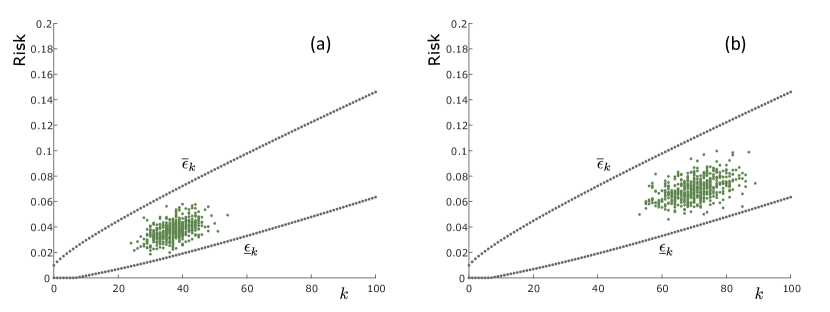
Figure 6: Region delimited by $\underline{\varepsilon}_{k}$ and $\overline{\varepsilon}_{k}$ for $N=1000$ and $\delta=10^{-3}$. The green dots are generated by a Monte-Carlo testing with (a) a Gaussian distribution and (b) a uniform distribution.

Panels (a) and (b) in Figure 6 profile the region delimited by $\underline{\varepsilon}_{k}$ and $\overline{\varepsilon}_{k}$ for $N=1000$ and $\delta=10^{-3}$. The green dots have coordinates equal to the cardinality of the compressed multiset ($x$ axis) and the risk ($y$ axis) in a Monte-Carlo testing in which points in ${{\mathbb{R}}^{3}}$ have a Gaussian distribution – panel (a) – and a uniform distribution in a hyper-cube – panel (b). One sees that the two clouds of green dots in (a) and in (b) are quite different, while, in both cases, they belong to the region (compare with the discussion in Section 2). Moreover, the stochastic fluctuation of the two clouds well covers the gap between the lower and the upper bound, signifying that the bounds are tight. $\star$

Remark 21

(On the role of observations) We feel advisable to just touch upon here an aspect, the full study of which goes beyond the intended goal of this paper. In data-driven applications, it is common practice that observations are split in two sets, used respectively for training and testing. This paper shows that, in a compression setup, data can well stand a double role, in which they are all used for training, while preserving their usability in the process of assessing the risk. Indeed, under the assumptions of Theorem 19 one can show that the quality of risk assessment by means of $\underline{\varepsilon}_{k}$ and $\overline{\varepsilon}_{k}$ (which is based on the sample of data points that has been used for training) only marginally degrades as compared to testing the solution with a new, untouched, sample of data points of equal cardinality. Hence, in this context, saving data for testing seems inappropriate, particularly when data are a scarce or costly resource. $\star$

For the non-consistent framework, it is interesting to further contrast asymptotic bounds that stem from the theory of this paper with previous results. To facilitate the comparison, we first reformulate our upper bound in terms of the empirical probability of inappropriateness $\hat{\mathsf{R}}\big{(}\mathcal{A}({\boldsymbol{S}})\big{)}$ (empirical risk). Start by noticing that $|\tilde{\mathsf{c}}({\boldsymbol{S}})|$ in Theorem 17 can be bounded as follows: $|\tilde{\mathsf{c}}({\boldsymbol{S}})|\leq\hat{\mathsf{R}}\big{(}\mathcal{A}({\boldsymbol{S}})\big{)}N+|\mathsf{c}({\boldsymbol{S}})|$ (strict inequality occurs when one or more examples ${\boldsymbol{z}}_{i}$ are simultaneously inappropriate and also contained in $\mathsf{c}({\boldsymbol{S}})$ and, therefore, counted twice in the right-hand side). Then, Theorem 17 in conjunction with Proposition 8 give, with probability $1-\delta$ with respect to the draw of the training set, that

$$\mathsf{R}\big{(}\mathcal{A}({\boldsymbol{S}})\big{)}$$ (13)

$$\leq \hat{\mathsf{R}}\big{(}\mathcal{A}({\boldsymbol{S}})\big{)}+\frac{|\mathsf{c}({\boldsymbol{S}})|}{N}$$

$$+2\frac{\sqrt{\hat{\mathsf{R}}\big{(}\mathcal{A}({\boldsymbol{S}})\big{)}N+|\mathsf{c}({\boldsymbol{S}})|+1}}{N}\left(\sqrt{\ln\left(\hat{\mathsf{R}}\big{(}\mathcal{A}({\boldsymbol{S}})\big{)}N+|\mathsf{c}({\boldsymbol{S}})|+1\right)}+4\right)$$

$$+2\frac{\sqrt{\hat{\mathsf{R}}\big{(}\mathcal{A}({\boldsymbol{S}})\big{)}N+|\mathsf{c}({\boldsymbol{S}})|+1}\sqrt{\ln\frac{1}{\delta}}}{N}+\frac{\ln\frac{1}{\delta}}{N}$$

$$= \hat{\mathsf{R}}\big{(}\mathcal{A}({\boldsymbol{S}})\big{)}+\frac{|\mathsf{c}({\boldsymbol{S}})|}{N}+$$

$${\scalebox{1.3}{$O$}\left({\left(\frac{\sqrt{\hat{\mathsf{R}}\big{(}\mathcal{A}({\boldsymbol{S}})\big{)}}}{\sqrt{N}}+\frac{\sqrt{|\mathsf{c}({\boldsymbol{S}})|+1}}{N}\right)\left(\sqrt{\ln\left(\hat{\mathsf{R}}\big{(}\mathcal{A}({\boldsymbol{S}})\big{)}N+|\mathsf{c}({\boldsymbol{S}})|+1\right)}+1\right)}\right)}\quad$$

(since our use of the notation $O(\cdot)$ is not standard, we clarify that here and in (14) $g(N,\mathsf{c}({\boldsymbol{S}}),\hat{\mathsf{R}}(\mathcal{A}({\boldsymbol{S}})))=O(f(N,\mathsf{c}({\boldsymbol{S}}),\hat{\mathsf{R}}(\mathcal{A}({\boldsymbol{S}}))))$ means that there exist a constant $C$ and an $\bar{N}$ such that $g(N,\mathsf{c}({\boldsymbol{S}}),\hat{\mathsf{R}}(\mathcal{A}({\boldsymbol{S}})))\leq Cf(N,\mathsf{c}({\boldsymbol{S}}),\hat{\mathsf{R}}(\mathcal{A}({\boldsymbol{S}})))$ for all $\mathsf{c}({\boldsymbol{S}})\in\{0,\ldots,N\}$ and $\hat{\mathsf{R}}(\mathcal{A}({\boldsymbol{S}}))\in[0,1]$ when $N\geq\bar{N}$). This last expression can be compared with the best available result in the literature given by Theorem 17 in Hanneke and Kontorovich (2021), which yields

$$\mathsf{R}\big{(}\mathcal{A}({\boldsymbol{S}})\big{)}=\hat{\mathsf{R}}\big{(}\mathcal{A}({\boldsymbol{S}})\big{)}+{\scalebox{1.3}{$O$}\left({\frac{|\mathsf{c}({\boldsymbol{S}})|+1}{N}+\frac{\sqrt{\hat{\mathsf{R}}\big{(}\mathcal{A}({\boldsymbol{S}})\big{)}}\sqrt{|\mathsf{c}({\boldsymbol{S}})|+1}}{\sqrt{N}}}\right)}.$$ (14)

It stands out that in (13) term $\sqrt{\hat{\mathsf{R}}\big{(}\mathcal{A}({\boldsymbol{S}})\big{)}}$ does not multiply $\sqrt{|\mathsf{c}({\boldsymbol{S}})|+1}$, as it instead does in (14); moreover, $\sqrt{|\mathsf{c}({\boldsymbol{S}})|+1}$ is divided by $N$ instead of $\sqrt{N}$. As a consequence, it is easy to show that, if, e.g., $\hat{\mathsf{R}}\big{(}\mathcal{A}({\boldsymbol{S}})\big{)}$ is replaced by a constant (so as to accommodate typical non-consistent frameworks), then the rate provided by (13) outdoes that of (14) whenever $|\mathsf{c}({\boldsymbol{S}})|$ grows sub-linearly and faster than $\ln(N)$ (when $|\mathsf{c}({\boldsymbol{S}})|$ is slower than $\ln(N)$, the dominant term in (13) is of the type $O(\sqrt{\ln(N)}/\sqrt{N})$, whereas in (14) it is of the type $O(\sqrt{|\mathsf{c}({\boldsymbol{S}})|}/\sqrt{N})$). For instance, replacing $|\mathsf{c}({\boldsymbol{S}})|$ with $\sqrt{N}$ gives the rate $\sqrt{\ln(N)}/\sqrt{N}$ in (13) and the rate $1/N^{\frac{1}{4}}$ in (14).

To close, we finally mention an interesting implication of our result that has been kindly suggested to us by an anonymous reviewer. Suppose that in a binary classification problem a hypothesis is selected from a class $\mathcal{H}$ via a compression scheme that minimizes the empirical risk (such compression scheme is named “agnostic sample compression scheme for $\mathcal{H}$” in David et al., 2016b, Section 2; see also David et al., 2016a), and that this compression scheme is also preferent. Then, (13) and Lemma 3.2 in David et al. (2016b) give (with high probability with respect to the draw of the training set) that

$$\mathsf{R}\big{(}\mathcal{A}({\boldsymbol{S}})\big{)}=\inf_{h\in\mathcal{H}}\mathsf{R}\big{(}h\big{)}+\frac{|\mathsf{c}({\boldsymbol{S}})|}{N}+{\scalebox{1.3}{$O$}\left({\frac{\sqrt{\ln(N)}}{\sqrt{N}}}\right)}.$$ (15)

On the other hand, Theorem 5.2 in Anthony and Bartlett (1999) establishes a bound to the rate at which any hypotheses class $\mathcal{H}$ of Vapnik-Chernovenkis dimension $d$ can be learned:

$$\mathsf{R}\big{(}\mathcal{A}({\boldsymbol{S}})\big{)}-\inf_{h\in\mathcal{H}}\mathsf{R}\big{(}h\big{)}\geq\sqrt{\frac{d}{320\cdot N}}.$$ (16)

Considering classes $\mathcal{H}$ whose Vapnik-Chernovenkis dimension increases with $N$ more than $\ln(N)$, results (15) and (16) imply that these classes cannot admit preferent “agnostic sample compression schemes for $\mathcal{H}$” of a size that increases at a rate less than $\sqrt{d}\sqrt{N}$. This result is in contrast with the case of non-preferent “agnostic sample compression scheme for $\mathcal{H}$”, in which context David et al. (2016b) shows that schemes of smaller cardinality can be found.

4 Application to known learning schemes

The theory developed in Section 3 is here applied to well-known learning techniques: some algorithms within the family of support vector methods and then a more recent classification technique called Guaranteed Error Machine (GEM). In all these cases, Theorem 10 applies without restrictions, while the use of Theorem 19 requires some conditions on the probability distribution of the examples. The content of this section is also meant to illustrate the flexibility and usefulness of the theory of this paper and, in this light, additional schemes that are amenable to be analyzed within the framework of Section 3 are hinted upon at the end of the section.

4.1 Support Vector methods

4.1.1 Support Vector Machines

In supervised binary classification, an example $z$ is a pair $z:=(x,y)$, where $x\in\mathcal{X}$ (think of $\mathcal{X}$ as a generic space without any specific structure) is an “instance” and $y\in\{-1,1\}$ is a “label”. A hypothesis, called a “binary classifier”, is a map $h:\mathcal{X}\to\{-1,1\}$. We let $\ell(h,(x,y))=\mathbbm{1}_{y\neq h(x)}$, so that the loss function equals $0$ when $y=h(x)$ (correct classification) and $1$ when $y\neq h(x)$ (misclassification).

To add flexibility, support vector methods are often got to operate in a feature space. Let $\varphi:\mathcal{X}\to\mathcal{H}$ be a “feature map” from $\mathcal{X}$ into a Hilbert space $\mathcal{H}$ equipped with an inner product $\langle\cdot,\cdot\rangle$. Support Vector Machine (SVM, see Cortes and Vapnik, 1995; Schölkopf and Smola, 1998) is a learning algorithm $\mathcal{A}_{\scriptscriptstyle{\mathrm{SVM}}}$ that maps a training set $S=\mathsf{ms}((x_{1},y_{1}),\ldots,(x_{n},y_{n}))$ into a binary classifier according to the formula

$$\mathcal{A}_{\scriptscriptstyle{\mathrm{SVM}}}(S)(x)=\begin{cases}1,&\text{if }\langle w^{\ast}(S),\varphi(x)\rangle+b^{\ast}(S)\geq 0\\ -1,&\text{if }\langle w^{\ast}(S),\varphi(x)\rangle+b^{\ast}(S)<0,\end{cases}$$

where $x$ is a generic instance and $(w^{\ast}(S),b^{\ast}(S))$ (along with the auxiliary variables $\xi_{i}^{\ast}(S)$ that are used to relax the constraint of exact classification of all the examples in the training set) is the solution to the optimization program

$$\mathcal{P}_{\scriptscriptstyle{\mathrm{SVM}}}(S): \displaystyle\min_{w\in\mathcal{H},b\in\mathbb{R}\atop\xi_{i}\geq 0,i=1,\ldots,n} \quad\displaystyle\|w\|^{2}+\rho\sum_{i=1}^{n}\xi_{i}$$

subject to: $$\displaystyle\quad 1-y_{i}(\langle w,\varphi(x_{i})\rangle+b)\leq\xi_{i},\ \ i=1,\ldots,n.$$

As shown in Theorem 2 in Burges and Crisp (1999), (4.1.1) always admits a minimizer and, moreover, $w^{\ast}(S)$ is unique; however, $b^{\ast}(S)$ (and $\xi^{\ast}_{i}(S)$) need not be unique. When $b^{\ast}(S)$ is not unique, we assume that the tie is broken by selecting the value of $b$ that minimizes $|b|$. Note that once $w^{\ast}(S)$ and $b^{\ast}(S)$ are uniquely determined, then also the optimal values $\xi^{\ast}_{i}(S)$ remain univocally identified.

As is well known, see e.g. Schölkopf and Smola (1998), the feature map $\varphi(\cdot)$ and the inner product $\langle\cdot,\cdot\rangle$ need not be explicitly assigned to solve (4.1.1). The reason is that the determination of the solution to (4.1.1) (as well as the evaluation of $\mathcal{A}_{\scriptscriptstyle{\mathrm{SVM}}}(S)(x)$) only involves the computation of inner products of the type $\langle\varphi(x_{i}),\varphi(x_{j})\rangle$ and $\langle\varphi(x_{i}),\varphi(x)\rangle$. These inner products can indeed be directly obtained from a kernel $k(\cdot,\cdot)$ ($k(\cdot,\cdot)$ is a function $\mathcal{X}\times\mathcal{X}\to\mathbb{R}$ that satisfies suitable conditions of positive definiteness, see Schölkopf and Smola, 1998) and the theory of Reproducing Kernel Hilbert Spaces ensures that any choice of $k(\cdot,\cdot)$ always corresponds to allocate a suitable pair $\varphi(\cdot)$, $\langle\cdot,\cdot\rangle$ so that $k(\cdot,\cdot)=\langle\varphi(\cdot),\varphi(\cdot)\rangle$ (this is the so-called “kernel trick”). We also note that the solution to (4.1.1) is typically obtained by solving a program that is the dual of (4.1.1). However, although important for the practice of SVM, all these remarks are immaterial for the discussion that follows.

To cast SVM within the framework of the present paper, introduce the following compression function $\mathsf{c}_{\scriptscriptstyle{\mathrm{SVM}}}$. First, endow $\mathcal{X}$ with an arbitrary total ordering (to be used below in point (ii)). For any multiset $S$, define $\mathsf{c}_{\scriptscriptstyle{\mathrm{SVM}}}(S)=S_{+}\cup S_{0}$ where:

• $S_{+}$ is the sub-multiset of all the examples (repeated as many times as they appear in $S$) for which $1-y_{i}(\langle w^{\ast}(S),\varphi(x_{i})\rangle+b^{\ast}(S))>0$ (note that this is equivalent to the condition $\xi^{\ast}_{i}(S)>0$);

• consider the sub-multisets $\tilde{S}_{0}$ of smallest cardinality for which:

  • $1-y_{i}(\langle w^{\ast}(S),\varphi(x_{i})\rangle+b^{\ast}(S))=0$; and,

  • the couple $(w^{\ast}(S_{+}\cup\tilde{S}_{0}),b^{\ast}(S_{+}\cup\tilde{S}_{0}))$ given by (4.1.1) with $S_{+}\cup\tilde{S}_{0}$ in place of the original $S$ is the same as $(w^{\ast}(S),b^{\ast}(S))$.

  Among the multisets $\tilde{S}_{0}$, single out $S_{0}$ by using the ordering on $\mathcal{X}$: for each candidate multiset $\tilde{S}_{0}$, identify the element with smallest instance and pick the multiset that exhibits the smallest among all; if a tie remains, move on to compare the second smallest and so on until $S_{0}$ is uniquely determined.

We want to apply Theorem 10 to SVM. To this purpose, we start by verifying that $\mathsf{c}_{\scriptscriptstyle{\mathrm{SVM}}}$ satisfies the preference Property 2.

$\diamond$ Preference. We apply Lemma 3, which requires to show that, for every multisets $S$ and $S^{\prime}$ such that $\mathsf{c}_{\scriptscriptstyle{\mathrm{SVM}}}(S)\subseteq S^{\prime}\subseteq S$, it holds that $\mathsf{c}_{\scriptscriptstyle{\mathrm{SVM}}}(S^{\prime})=\mathsf{c}_{\scriptscriptstyle{\mathrm{SVM}}}(S)$.
First, we show that

$$(w^{\ast}(S^{\prime}),b^{\ast}(S^{\prime}))=(w^{\ast}(S),b^{\ast}(S)).$$ (18)

For the sake of contradiction, suppose that (18) does not hold:

$$(w^{\ast}(S^{\prime}),b^{\ast}(S^{\prime}))\neq(w^{\ast}(S),b^{\ast}(S)).$$ (19)

Note that the value achieved by $(w^{\ast}(S^{\prime}),b^{\ast}(S^{\prime}))$ for the problem that only contains the constraints corresponding to the examples in $\mathsf{c}_{\scriptscriptstyle{\mathrm{SVM}}}(S)$ cannot be worse than the value achieved by $(w^{\ast}(S^{\prime}),b^{\ast}(S^{\prime}))$ for the problem containing the constraints associated to $S^{\prime}$ (because the latter is more constrained than the former); moreover, the value achieved by $(w^{\ast}(S),b^{\ast}(S))$ for the problem containing only the constraints associated to $\mathsf{c}_{\scriptscriptstyle{\mathrm{SVM}}}(S)$ is equal to the value achieved by $(w^{\ast}(S),b^{\ast}(S))$ for the problem containing the constraints associated to $S^{\prime}$ (because the examples in $S^{\prime}$ that are not in $\mathsf{c}_{\scriptscriptstyle{\mathrm{SVM}}}(S)$ corresponds to $\xi_{i}^{\ast}(S)$ whose value is zero). From (19), then, one concludes that $(w^{\ast}(S^{\prime}),b^{\ast}(S^{\prime}))$ must be preferred to $(w^{\ast}(S),b^{\ast}(S))$ for the problem containing only the constraints associated to $\mathsf{c}_{\scriptscriptstyle{\mathrm{SVM}}}(S)$. This, however, leads to a contradiction because, by construction $(w^{\ast}(\mathsf{c}_{\scriptscriptstyle{\mathrm{SVM}}}(S)),b^{\ast}(\mathsf{c}_{\scriptscriptstyle{\mathrm{SVM}}}(S)))=(w^{\ast}(S),b^{\ast}(S))$. Hence, (18) remains proven.
Consider now $\mathsf{c}_{\scriptscriptstyle{\mathrm{SVM}}}(S^{\prime})=S^{\prime}_{+}\cup S^{\prime}_{0}$, where $S^{\prime}_{+}$ and $S^{\prime}_{0}$ are obtained from (i) and (ii) applied to $S^{\prime}$. Since $S^{\prime}\supseteq\mathsf{c}_{\scriptscriptstyle{\mathrm{SVM}}}(S)$, $S^{\prime}$ contains all the examples in $S$ for which $1-y_{i}(\langle w^{\ast}(S),\varphi(x_{i})\rangle+b^{\ast}(S))>0$ and, in view of (18), these examples are also all those in $S^{\prime}$ for which $1-y_{i}(\langle w^{\ast}(S^{\prime}),\varphi(x_{i})\rangle+b^{\ast}(S^{\prime}))>0$. Thus, $S^{\prime}_{+}=S_{+}$. The fact that $S^{\prime}_{0}=S_{0}$ follows instead from observing that $S_{0}$ is the preferred selection according to the ordering procedure in (ii) to recover $(w^{\ast}(S),b^{\ast}(S))$ and, since $(w^{\ast}(S^{\prime}),b^{\ast}(S^{\prime}))=(w^{\ast}(S),b^{\ast}(S))$ and $S_{0}$ is available as a sub-multiset of $S^{\prime}$, this same $S_{0}$ is selected when (ii) is applied to $S^{\prime}$, leading to $S^{\prime}_{0}=S_{0}$. This establishes the validity of Lemma 3 and closes the argument. $\star$

Next, we verify the coherence – part I Property 9.

$\diamond$ Coherence – part I. Notice first that the very definition of $\mathsf{c}_{\scriptscriptstyle{\mathrm{SVM}}}$ implies that $\mathcal{A}_{\scriptscriptstyle{\mathrm{SVM}}}(\mathsf{c}_{\scriptscriptstyle{\mathrm{SVM}}}(S))\break=\mathcal{A}_{\scriptscriptstyle{\mathrm{SVM}}}(S)$, i.e., $\mathcal{A}_{\scriptscriptstyle{\mathrm{SVM}}}$ itself acts as a reconstruction function. Moreover, if we have that $\ell(\mathcal{A}_{\scriptscriptstyle{\mathrm{SVM}}}(S),(x_{i},y_{i}))=1$ for an example $(x_{i},y_{i})$ in $S$, then it must be that $y_{i}(\langle w^{\ast}(S),\varphi(x_{i})\rangle+b^{\ast}(S))\leq 0$ (because $y_{i}$ has sign opposite to that of $\langle w^{\ast}(S),\varphi(x_{i})\rangle+b^{\ast}(S)$). This implies that $1-y_{i}(\langle w^{\ast}(S),\varphi(x_{i})\rangle+b^{\ast}(S))>0$, from which the inclusion Property 12 follows because $\mathsf{c}_{\scriptscriptstyle{\mathrm{SVM}}}(S)$ includes all examples for which this latter inequality holds true. Based on these results, the coherence – part I Property 9 follows from Lemma 13. $\star$

Having established the preference and the coherence - part I properties, the following theorem follows as a corollary of Theorem 10.

Theorem 22

(Risk of SVM) For any $\delta\in(0,1)$, it holds that

$${\mathbb{P}}\Big{\{}\mathsf{R}\big{(}\mathcal{A}_{\scriptscriptstyle{\mathrm{SVM}}}({\boldsymbol{S}})\big{)}>\varepsilon_{\boldsymbol{k}}\Big{\}}\leq\delta,$$

where ${\boldsymbol{k}}=|\mathsf{c}_{\scriptscriptstyle{\mathrm{SVM}}}({\boldsymbol{S}})|$ and $\varepsilon_{k}$ is given in (1). $\star$

We are instead not in a position to establish lower bounds for $\mathsf{R}\big{(}\mathcal{A}_{\scriptscriptstyle{\mathrm{SVM}}}({\boldsymbol{S}})\big{)}$. The reason is that adding a new example $(x_{n+1},y_{n+1})$ for which $1-y_{n+1}(\langle w^{\ast}(S),\varphi(x_{n+1})\rangle+b^{\ast}(S))>0$ changes the compression (refer to (i) in the definition of $\mathsf{c}_{\scriptscriptstyle{\mathrm{SVM}}}$), but this does not exclude that $y_{n+1}(\langle w^{\ast}(S),\varphi(x_{n+1})\rangle+b^{\ast}(S))>0$, in which case the new example is not misclassified. This fact prevents the coherence – part II Property 18 from being satisfied.

Remark 23

(A computational aspect) To evaluate an upper bound to the risk according to Theorem 22, one needs to compute $|\mathsf{c}_{\scriptscriptstyle{\mathrm{SVM}}}(S)|$. Computing the cardinality of $S_{+}$ is easy; determining the cardinality of $S_{0}$, however, is more computationally demanding. On the other hand, $\varepsilon_{k}$ is increasing with $k$ so that a valid result can be easily found by overestimating $|\mathsf{c}_{\scriptscriptstyle{\mathrm{SVM}}}(S)|$ with the cardinality of the set of examples for which $1-y_{i}(\langle w^{\ast}(S),\varphi(x_{i})\rangle+b^{\ast}(S))\geq 0$. Heuristically, this evaluation often turns out to be sharp. $\star$

4.1.2 Support Vector Regression

In regression problems, an example $z$ is a pair $z:=(x,y)$ with $x\in\mathcal{X}$, a generic space, and $y\in\mathbb{R}$. A hypothesis $h$ is called a “predictor” and it is a map from $\mathcal{X}$ to $\mathbb{R}$. As loss function, we take

$$\ell(h,(x,y))=\begin{cases}1,&\text{if }|y-h(x)|>t\\ 0,&\text{if }|y-h(x)|\leq t,\end{cases}$$

where $t$ is the so-called “prediction tolerance”. Let $\varphi:\mathcal{X}\to\mathcal{H}$ be a feature map from $\mathcal{X}$ to a Hilbert space $\mathcal{H}$ endowed with inner product $\langle\cdot,\cdot\rangle$. Support Vector Regression (SVR, see Smola and Schölkopf, 2004) is a learning algorithm $\mathcal{A}_{\scriptscriptstyle{\mathrm{SVR}}}(S)$ that maps any training set $S=\mathsf{ms}((x_{1},y_{1}),\ldots,(x_{n},y_{n}))$ into the predictor

$$\mathcal{A}_{\scriptscriptstyle{\mathrm{SVR}}}(S)(x)=\langle w^{\ast}(S),\varphi(x)\rangle+b^{\ast}(S)$$

where $w^{\ast}(S)$ and $b^{\ast}(S)$ (along with $\xi_{i}^{\ast}(S)$) are the solution to the program

$$\mathcal{P}_{\scriptscriptstyle{\mathrm{SVR}}}(S): \displaystyle\min_{w\in\mathcal{H},b\in\mathbb{R}\atop\xi_{i}\geq 0,i=1,\ldots,n} \displaystyle\quad\|w\|^{2}+\rho\sum_{i=1}^{n}\xi_{i}$$

subject to: $$\displaystyle\quad|y_{i}-\langle w,\varphi(x_{i})\rangle-b|\leq t+\xi_{i},\ \ i=1,\ldots,n.$$

Similarly to SVM, a minimizer certainly exists and $w^{\ast}(S)$ is also unique, but $b^{\ast}(S)$ may not be, see Burges and Crisp (1999). In the latter case, the tie is broken by choosing the minimizer with the smallest value of $|b|$. After that $w^{\ast}(S)$ and $b^{\ast}(S)$ have been made unique, also the values of $\xi_{i}^{\ast}(S)$ remain univocally determined. The kernel trick described for SVM applies here as well, so that $\varphi(\cdot)$ and $\langle\cdot,\cdot\rangle$ need not be specified explicitly and can be assigned via a kernel function.

Our definition of a compression function $\mathsf{c}_{\scriptscriptstyle{\mathrm{SVR}}}$ closely resembles that for SVM. For any multiset of examples $S$, define $\mathsf{c}_{\scriptscriptstyle{\mathrm{SVR}}}(S)=S_{+}\cup S_{0}$ where:

• $S_{+}$ is the multiset of all the examples (repeated as many times as they appear in $S$) for which $|y_{i}-\langle w^{\ast}(S),\varphi(x_{i})\rangle-b^{\ast}(S)|>t$ (note that this is equivalent to the condition $\xi^{\ast}_{i}(S)>0$);

• $S_{0}$ is the smallest sub-multiset only containing examples that satisfy condition $|y_{i}-\langle w^{\ast}(S),\varphi(x_{i})\rangle-b^{\ast}(S)|=t$ for which $w^{\ast}(S_{+}\cup S_{0})=w^{\ast}(S)$ and $b^{\ast}(S_{+}\cup S_{0})=b^{\ast}(S)$. In complete analogy with SVM, $S_{0}$ as defined before may not be unique, in which case an $S_{0}$ is singled out by a total ordering on $\mathcal{X}$.

The proof that $\mathsf{c}_{\scriptscriptstyle{\mathrm{SVR}}}$ satisfies the preference Property 2 and that $(\mathcal{A}_{\scriptscriptstyle{\mathrm{SVR}}},\mathsf{c}_{\scriptscriptstyle{\mathrm{SVR}}})$ satisfies the coherence – part I Property 9 follows the same path, mutatis mutandis, as for SVM and is therefore omitted. This gives the following theorem, obtained as a direct consequence of Theorem 10.

Theorem 24

(Risk of SVR) For any $\delta\in(0,1)$, it holds that

$${\mathbb{P}}\Big{\{}\mathsf{R}\big{(}\mathcal{A}_{\scriptscriptstyle{\mathrm{SVR}}}({\boldsymbol{S}})\big{)}>\varepsilon_{\boldsymbol{k}}\Big{\}}\leq\delta,$$

where ${\boldsymbol{k}}=|\mathsf{c}_{\scriptscriptstyle{\mathrm{SVR}}}({\boldsymbol{S}})|$ and $\varepsilon_{k}$ is given in (1). $\star$

Unlike SVM, for SVR lower and upper bounds for the risk are established under an additional, mild, distributional assumption.

Assumption 25

The regular conditional distribution of ${\boldsymbol{y}}$ given ${\boldsymbol{x}}$ has no concentrated mass almost surely. $\star$

To establish the lower and upper bounds, we resort to Theorem 19. Preliminarily, we show the validity of the assumptions of this theorem.

$\diamond$ Non-associativity. Consider any training set $S=\mathsf{ms}((x_{1},y_{1}),\ldots,(x_{n},y_{n}))$ and an additional multiset of examples $S^{\prime}=\mathsf{ms}((x_{n+1},y_{n+1}),\ldots,(x_{n+p},y_{n+p}))$ such that $\mathsf{c}(S,(x_{n+i},\break y_{n+i}))=\mathsf{c}(S)$ for all $i\in\{1,\ldots,p\}$. Further, assume that $|y_{n+i}-\mathcal{A}_{\scriptscriptstyle{\mathrm{SVR}}}(S)(x_{n+i})|\neq t$ for all $i\in\{1,\ldots,p\}$. Then, it must be that $|y_{n+i}-\mathcal{A}_{\scriptscriptstyle{\mathrm{SVR}}}(S)(x_{n+i})|<t$ for all $i\in\{1,\ldots,p\}$. Indeed, suppose by contradiction the opposite: $|y_{n+i}-\mathcal{A}_{\scriptscriptstyle{\mathrm{SVR}}}(S)(x_{n+i})|>t$ for some $i$. Then, if $\mathcal{A}_{\scriptscriptstyle{\mathrm{SVR}}}(S,(x_{n+i},y_{n+i}))=\mathcal{A}_{\scriptscriptstyle{\mathrm{SVR}}}(S)$, then $|y_{n+i}-\mathcal{A}_{\scriptscriptstyle{\mathrm{SVR}}}(S,(x_{n+i},y_{n+i}))(x_{n+i})|>t$ and $(x_{n+i},y_{n+i})$ is counted in $\mathsf{c}_{\scriptscriptstyle{\mathrm{SVR}}}(S,(x_{n+i},y_{n+i}))$ leading to $\mathsf{c}_{\scriptscriptstyle{\mathrm{SVR}}}(S,(x_{n+i},y_{n+i}))\neq\mathsf{c}_{\scriptscriptstyle{\mathrm{SVR}}}(S)$; if instead $\mathcal{A}_{\scriptscriptstyle{\mathrm{SVR}}}(S,(x_{n+i},y_{n+i}))\neq\mathcal{A}_{\scriptscriptstyle{\mathrm{SVR}}}(S)$, then $\mathcal{A}_{\scriptscriptstyle{\mathrm{SVR}}}(\mathsf{c}_{\scriptscriptstyle{\mathrm{SVR}}}(S,(x_{n+i},y_{n+i})))\neq\mathcal{A}_{\scriptscriptstyle{\mathrm{SVR}}}(\mathsf{c}_{\scriptscriptstyle{\mathrm{SVR}}}(S))$, which means that $\mathsf{c}_{\scriptscriptstyle{\mathrm{SVR}}}(S,(x_{n+i},y_{n+i}))$ cannot be the same as $\mathsf{c}_{\scriptscriptstyle{\mathrm{SVR}}}(S)$. Thus, it remains proven that $|y_{n+i}-\mathcal{A}_{\scriptscriptstyle{\mathrm{SVR}}}(S)(x_{n+i})|<t$ for all $i\in\{1,\ldots,p\}$ and this yields immediately that $\mathcal{A}_{\scriptscriptstyle{\mathrm{SVR}}}(S\cup S^{\prime})=\mathcal{A}_{\scriptscriptstyle{\mathrm{SVR}}}(S)$ and that $\mathsf{c}_{\scriptscriptstyle{\mathrm{SVR}}}(S\cup S^{\prime})=\mathsf{c}_{\scriptscriptstyle{\mathrm{SVR}}}(S)$. This, along with the fact that $|{\boldsymbol{y}}_{n+i}-\mathcal{A}_{\scriptscriptstyle{\mathrm{SVR}}}({\boldsymbol{S}})({\boldsymbol{x}}_{n+i})|\neq t$ for all $i\in\{1,\ldots,p\}$ holds with probability $1$ in view of Assumption 25, gives the non-associativity property. $\star$

$\diamond$ Non-concentrated mass. This is obvious in view of Assumption 25. $\star$

$\diamond$ Coherence – part II. The proof is by contrapositive: letting ${\boldsymbol{S}}=\mathsf{ms}(({\boldsymbol{x}}_{1},{\boldsymbol{y}}_{1}),\ldots,({\boldsymbol{x}}_{n},{\boldsymbol{y}}_{n}))$ we show that

$${\mathbb{P}}\Big{(}\{\ell(\mathcal{A}_{\scriptscriptstyle{\mathrm{SVR}}}({\boldsymbol{S}}),({\boldsymbol{x}}_{n+1},{\boldsymbol{y}}_{n+1}))=0\}\setminus\{\mathsf{c}_{\scriptscriptstyle{\mathrm{SVR}}}(\mathsf{c}_{\scriptscriptstyle{\mathrm{SVR}}}({\boldsymbol{S}}),({\boldsymbol{x}}_{n+1},{\boldsymbol{y}}_{n+1}))=\mathsf{c}_{\scriptscriptstyle{\mathrm{SVR}}}({\boldsymbol{S}})\}\Big{)}=0.$$ (20)

Assumption 25 implies that the case $|y_{n+1}-\mathcal{A}_{\scriptscriptstyle{\mathrm{SVR}}}(S)(x_{n+1})|=t$ can be disregarded because it correpsonds to an event that has probability zero. Moreover, when $|y_{n+1}-\mathcal{A}_{\scriptscriptstyle{\mathrm{SVR}}}(S)(x_{n+1})|>t$, we have that $\ell(\mathcal{A}_{\scriptscriptstyle{\mathrm{SVR}}}(S),(x_{n+1},y_{n+1}))=1$, so that this case can be disregarded too. When instead $|y_{n+1}-\mathcal{A}_{\scriptscriptstyle{\mathrm{SVR}}}(S)(x_{n+1})|<t$, it holds that $\ell\big{(}\mathcal{A}_{\scriptscriptstyle{\mathrm{SVR}}}(S),(x_{n+1},\break y_{n+1})\big{)}=0$. In this case,

$$|y_{n+1}-\mathcal{A}_{\scriptscriptstyle{\mathrm{SVR}}}(\mathsf{c}_{\scriptscriptstyle{\mathrm{SVR}}}(S))(x_{n+1})|=|y_{n+1}-\mathcal{A}_{\scriptscriptstyle{\mathrm{SVR}}}(S)(x_{n+1})|<t$$

yields $\mathcal{A}_{\scriptscriptstyle{\mathrm{SVR}}}(\mathsf{c}_{\scriptscriptstyle{\mathrm{SVR}}}(S),(x_{n+1},y_{n+1}))=\mathcal{A}_{\scriptscriptstyle{\mathrm{SVR}}}(S)$, from which

$$|y_{n+1}-\mathcal{A}_{\scriptscriptstyle{\mathrm{SVR}}}(\mathsf{c}_{\scriptscriptstyle{\mathrm{SVR}}}(S),(x_{n+1},y_{n+1}))(x_{n+1})|<t.$$

Hence, $(x_{n+1},y_{n+1})$ is not in $\mathsf{c}_{\scriptscriptstyle{\mathrm{SVR}}}(\mathsf{c}_{\scriptscriptstyle{\mathrm{SVR}}}(S),(x_{n+1},y_{n+1}))$, so that, owing to the preference Property 2, it must be that $\mathsf{c}_{\scriptscriptstyle{\mathrm{SVR}}}(\mathsf{c}_{\scriptscriptstyle{\mathrm{SVR}}}(S),(x_{n+1},y_{n+1}))=\mathsf{c}_{\scriptscriptstyle{\mathrm{SVR}}}(S)$. This shows the validity of (20). $\star$

Using Theorem 19, we now have the following result.

Theorem 26

(Risk of SVR - bounds from below and from above) Under Assumption 25, for any $\delta\in(0,1)$, it holds that

$${\mathbb{P}}\Big{\{}\underline{\varepsilon}_{\boldsymbol{k}}\leq\mathsf{R}\big{(}\mathcal{A}_{\scriptscriptstyle{\mathrm{SVR}}}({\boldsymbol{S}})\big{)}\leq\overline{\varepsilon}_{\boldsymbol{k}}\Big{\}}\geq 1-\delta,$$

where ${\boldsymbol{k}}=|\mathsf{c}_{\scriptscriptstyle{\mathrm{SVR}}}({\boldsymbol{S}})|$ and $\underline{\varepsilon}_{k}$, $\overline{\varepsilon}_{k}$ are given respectively in (4), (5). $\star$

4.1.3 Other Support Vector methods

The applicability of Theorems 10 and 19 can be carried over to other Support Vector methods. SVR with Adjustable Size, Schölkopf et al. (1998), requires minor modifications. Suitable but conceptually straightforward modifications of the arguments used in this section can also be applied to one-class SVM, Schölkopf et al. (1999), and Support Vector Data Description (SVDD), Tax and Duin (2004) and Wang et al. (2011). In these latter two cases, the setup changes slightly since examples are unlabeled and hypotheses are regions in the set hosting the examples. To apply Theorem 19, one needs here to modify Assumption 25 so as to enforce specific non-accumulation conditions for the method at hand.

4.2 Guaranteed Error Machine

The Guaranteed Error Machine (GEM) is a learning algorithm for classification that was first introduced in Campi (2010) and then further developed in Caré et al. (2018). GEM returns a ternary-valued classifier, which is also allowed to abstain from classifying in case of doubt. To be specific, letting $z=(x,y)$ with $x\in\mathcal{X}$, a generic set, and $y\in\{-1,1\}$ (this is the same setup as in SVM), a hypothesis $h$ is here a map from $\mathcal{X}$ to $\{-1,1,0\}$, where the value $0$ is interpreted as admission of being unable to classify. Issuing an incorrect label ($-1$ in place of $1$ or vice versa) leads to a mistake, and the theory aims at bounding the probability for this to happen. Correspondingly, the loss function is defined as follows:

$$\ell(h,(x,y))=\begin{cases}1,&\text{if }|y-h(x)|=2\\ 0,&\text{if }|y-h(x)|=0\text{ or }1.\end{cases}$$

To describe the operation of GEM, start by introducing a feature map $\varphi:\mathcal{X}\to\mathcal{H}$, where $\mathcal{H}$ is a Hilbert space with inner product $\langle\cdot,\cdot\rangle$ (as for support vector methods, $\varphi$, $\mathcal{H}$, and $\langle\cdot,\cdot\rangle$ need not be explicitly given and can be implicitly defined by means of a kernel) and also assume the existence of an ordering on $\mathcal{X}$ (used later to introduce a tie-break rule). GEM requires that the user chooses an integer $d\geq 1$, which specifies the maximal cardinality for the compression. In loose terms, GEM operates as follows. It is assumed that one has an additional observation $(\bar{x},\bar{y})$ (besides the training set $S=\mathsf{ms}((x_{1},y_{1}),\ldots,(x_{n},y_{n}))$) that acts as initial “center”. GEM constructs the hyper-sphere in $\mathcal{H}$ around $\varphi(\bar{x})$ which is the largest possible under the condition that the hyper–sphere does not include any $\varphi(x_{i})$ with label $y_{i}$ different from $\bar{y}$. All points inside this hyper-sphere are classified as the label $\bar{y}$, and all examples $(x_{i},y_{i})$ for which $\varphi(x_{i})$ is inside the hyper-sphere are removed from the training set. The example that lies on the boundary of the hyper-sphere (and that has therefore prevented the hyper–sphere from further enlarging) is then appointed as the new center (in case of ties, the tie is broken by using the ordering on $\mathcal{X}$) and the procedure is repeated by constructing another hyper-sphere around the new center. This time, only the region given by the difference between the newly constructed hyper-sphere and the first hyper–sphere (which has been already classified) is classified as the label of the second center. This procedure continues the same way and comes to a stop when either the whole space has been classified or the total number of centers is equal to $d$, in which case the portion of $\mathcal{X}$ that has not been covered is classified as $0$. This leads to the algorithm formally described below.

• SET $q:=0$, $P:=S\cup\mathsf{ms}((\bar{x},\bar{y}))$, $C=\emptyset$ and $x_{C}=\bar{x}$, $y_{C}=\bar{y}$;

• SET $q:=q+1$ and SOLVE problem

  $$\displaystyle\max_{r\geq 0} r$$

  subject to: $$\|\varphi(x_{i})-\varphi(x_{C})\|\geq r,\text{ for all }(x_{i},y_{i})\in P\text{ such that }y_{i}\neq y_{C}.$$

  Let $r^{\ast}$ be the optimal solution (note that $r^{\ast}$ can possibly be $+\infty$);

• FORM the region $\mathcal{R}_{q}:=\{x\in\mathcal{X}:\;\|\varphi(x)-\varphi(x_{C})\|<r^{\ast}\}$ and LET $\ell_{q}:=y_{C}$; UPDATE $P$ as follows: if $r^{\ast}>0$, then remove from $P$ all the examples with $x_{i}\in\mathcal{R}_{q}$; if instead $r^{\ast}=0$, then remove from $P$ the example $(x_{C},y_{C})$;

• IF $r^{\ast}<+\infty$, THEN

  • SET $C:=C\cup\mathsf{ms}((x_{i^{\ast}},y_{i^{\ast}}))$, where $(x_{i^{\ast}},y_{i^{\ast}})$ is an example in $P$ such that: a. $\|\varphi(x_{i^{\ast}})-\varphi(x_{C})\|=r^{\ast}$; b. $y_{i^{\ast}}\neq y_{C}$; c. $x_{i^{\ast}}$ is smallest in the ordering of $\mathcal{X}$ among all the examples satisfying a. and b.;

  • SET $(x_{C},y_{C}):=(x_{i^{\ast}},y_{i^{\ast}})$;

• IF either $|C|=d$ or $P=\emptyset$ THEN STOP and RETURN $\ell_{j}$, $\mathcal{R}_{j}$, $j=1,\ldots,q$ and $C$;
  ELSE, GO TO 1.

The GEM predictor is defined as

$$\mathcal{A}_{\scriptscriptstyle{\mathrm{GEM}}}(S)(x)=\begin{cases}0,&\quad\text{if }x\notin\mathcal{R}_{j}\;\forall j=1,\ldots,q;\\ \ell_{j^{\ast}}&\quad\text{otherwise, with }j^{\ast}=\min\big{\{}j\in\{1,\ldots,q\}:\;x\in\mathcal{R}_{j}\big{\}}.\end{cases}$$

The compression function for GEM is $\mathsf{c}_{\scriptscriptstyle{\mathrm{GEM}}}(S)=C$.

We next establish the preference and coherence – part I properties, required to apply Theorem 10.

$\diamond$ Preference. Given any multisets $S$ and $S^{\prime}$ such that $\mathsf{c}_{\scriptscriptstyle{\mathrm{GEM}}}(S)\subseteq S^{\prime}\subseteq S$, it is easy to verify that running STEPS 0-4 with $S^{\prime}$ as input returns the same output as when these steps are run with input $S$. In particular, $\mathsf{c}_{\scriptscriptstyle{\mathrm{GEM}}}(S^{\prime})=C=\mathsf{c}_{\scriptscriptstyle{\mathrm{GEM}}}(S)$ and, therefore, the preference property follows by an application of Lemma 3. $\star$

$\diamond$ Coherence – part I. Since applying STEPS 0-4 to $\mathsf{c}_{\scriptscriptstyle{\mathrm{GEM}}}(S)$ returns the same output as when they are applied to $S$, $\mathcal{A}_{\scriptscriptstyle{\mathrm{GEM}}}$ itself acts as a reconstruction function. Also, the inclusion Property 12 is immediately verified (just pay a bit of care to the case in which more examples with different labels corresponds to the same $x_{C}$). The coherence – part I Property 9 then follows from Lemma 13. $\star$

Applying Theorem 10 we now have the following result.

Theorem 27

(Risk of GEM) For any $\delta\in(0,1)$, it holds that

$${\mathbb{P}}\Big{\{}\mathsf{R}\big{(}\mathcal{A}_{\scriptscriptstyle{\mathrm{GEM}}}({\boldsymbol{S}})\big{)}>\varepsilon_{\boldsymbol{k}}\Big{\}}\leq\delta,$$

where ${\boldsymbol{k}}=|\mathsf{c}_{\scriptscriptstyle{\mathrm{GEM}}}({\boldsymbol{S}})|$ and $\varepsilon_{k}$ is given in (1). $\star$

Notice also that $|\mathsf{c}_{\scriptscriptstyle{\mathrm{GEM}}}({\boldsymbol{S}})|\leq d$ holds by construction, which implies that the bound $\mathsf{R}\big{(}\mathcal{A}_{\scriptscriptstyle{\mathrm{GEM}}}({\boldsymbol{S}})\big{)}\leq\varepsilon_{d}$ is always correct with high confidence $1-\delta$.

We now turn to lower bounds to the risk, which are established by an application of Theorem 19. We start by showing the validity of the non-associativity property.

$\diamond$ Non-associativity. Consider any training set $S=\mathsf{ms}((x_{1},y_{1}),\ldots,(x_{n},y_{n}))$ and an additional multiset of examples $S^{\prime}=\mathsf{ms}((x_{n+1},y_{n+1}),\ldots,(x_{n+p},y_{n+p}))$. Suppose that $\mathsf{c}_{\scriptscriptstyle{\mathrm{GEM}}}(S\cup S^{\prime})\neq\mathsf{c}_{\scriptscriptstyle{\mathrm{GEM}}}(S)$. For this to be, it is required that at least one of these conditions applies: (i) $\ell(\mathcal{A}_{\scriptscriptstyle{\mathrm{GEM}}}(S),(x_{n+i},y_{n+i}))=1$ for some $i\in\{1,\ldots,p\}$; or, (ii) one of the $(x_{n+i},y_{n+i})$, $i\in\{1,\ldots,p\}$, for which $\ell(\mathcal{A}_{\scriptscriptstyle{\mathrm{GEM}}}(S),(x_{n+i},y_{n+i}))=0$ lies on the boundary of a $\mathcal{R}_{j}$ and is lower in order than the example that is chosen as center by the algorithm applied to $S$. However, take in isolation an example $(x_{n+i},y_{n+i})$ that satisfies either (i) or (ii); then, that example alone makes the compression change. This proves the non-associativity property. $\star$

To move on and prove the non-concentrated mass and coherence – part II properties, we need a mild assumption on the distribution of examples.

Assumption 28

For any $c\in\mathcal{H}$ and $\gamma\in{{\mathbb{R}}}$, it holds that

$${\mathbb{P}}\{\|\varphi({{\boldsymbol{x}}})-c\|^{2}=\gamma\}=0.$$

$\star$

$\diamond$ Non-concentrated mass. This immediately follows from Assumption 28: if ${\mathbb{P}}\{{\boldsymbol{z}}=\bar{z}\}\neq 0$ for some $\bar{z}=(\bar{x},\bar{y})$, then Assumption 28 is violated by the choices $c=\varphi(\bar{x})$ and $\gamma=0$. $\star$

$\diamond$ Coherence – part II. In view of Assumption 28, ${\boldsymbol{x}}_{n+1}$ lies on the boundary of a region $\mathcal{R}_{j}$ with probability zero. On the other hand, when $x_{n+1}$ is not on the boundary, a change of compression only occurs if $(x_{n+1},y_{n+1})$ is misclassified, that is, $\ell(\mathcal{A}_{\scriptscriptstyle{\mathrm{GEM}}}(S),(x_{n+1},y_{n+1}))=1$. This proves the coherence – part II property. $\star$

The following theorem now follows from Theorem 19.

Theorem 29

(Risk of GEM - bounds from below and from above) Under Assumption 28, for any $\delta\in(0,1)$, it holds that

$${\mathbb{P}}\Big{\{}\underline{\varepsilon}_{\boldsymbol{k}}\leq\mathsf{R}\big{(}\mathcal{A}_{\scriptscriptstyle{\mathrm{GEM}}}({\boldsymbol{S}})\big{)}\leq\overline{\varepsilon}_{\boldsymbol{k}}\Big{\}}\geq 1-\delta,$$

where ${\boldsymbol{k}}=|\mathsf{c}_{\scriptscriptstyle{\mathrm{GEM}}}({\boldsymbol{S}})|$ and $\underline{\varepsilon}_{k}$, $\overline{\varepsilon}_{k}$ are given respectively in (4), (5). $\star$

4.3 Other learning schemes with a preferent compression

Besides Support Vector methods and GEM, other learning schemes can be studied within the framework of the present paper. We mention here just two additional examples, without working out all the details as it was done in Sections 4.1 and 4.2.

One first example is the class of methods for classification based on the nearest-neighbor (NN) algorithm. Consider for simplicity $1$-NN in a finite Euclidean space $\mathcal{X}$ and with labels generated by a target concept, see Shalev-Shwartz and Ben-David (2014). For every training set $S=\mathsf{ms}((x_{1},y_{1}),\ldots,(x_{n},y_{n}))$ of instance/label pairs, $1$-NN relies on the Voronoi partition of the instance domain $\mathcal{X}$ induced by $S$, where cells are $C_{i}=\{x\in\mathcal{X}:\|x-x_{i}\|\leq\|x-x_{j}\|\;\forall j=1,\ldots,n\}$, $i=1,\ldots,n$. If one eliminates from $S$ all the examples whose associated cell is in the interior of the region labeled as the cell, then the remaining examples form a compressed multiset for which $1$-NN itself acts as a reconstruction function. It is then a simple enough task to show that such a compression function satisfies the preference Property 2; moreover, since the $1$-NN classifier is always consistent with $S$, Lemma 13 allows us to conclude that the coherence – part I Property 9 holds. Thereby, Theorem 10 can be applied to evaluate the probability of misclassification of the $1$-NN classifier. Similar arguments are expected to be applicable to more general $k$-NN schemes, even in generic (infinite dimensional) metric spaces. Further studies can possibly cover more general NN-based methods along the lines of Kontorovich et al. (2017, 2018); Hanneke et al. (2021).

As a second example, again in the context of classification, we would like to mention the Total Recall algorithm of Helmbold et al. (1990), which is in use to learn nested differences of concepts from intersection-closed classes. In the setup of Helmbold et al. (1990), no matter whether the depth of the hypothesis returned by the algorithm is arbitrary or a-priori fixed, it is fairly easy to prove that the union of the spanning sets with minimal cardinality for the multisets of examples used in the various calls to the closure learner by the Total Recall algorithm defines a compression function that satisfies the preference Property 2. By the very definition of spanning sets, we also have that the Total Recall algorithm applied to the union of the minimal spanning sets (i.e., applied to the compressed multiset) returns the same hypothesis as when the algorithm is run on the whole training set. This means that the Total Recall algorithm itself acts as a reconstruction function and Theorem 17 can be used to obtain evaluations of the probability of misclassification. More research can extend this analysis to alternative algorithms, e.g., along the lines discussed in Section 5 in Helmbold et al. (1990).

5 Proofs

5.1 A brief overview of the proofs

To help readability, we first trace a roadmap of the fundamental steps in which the rather long proofs of Theorems 4 and 7 are articulated. To prove Theorem 4, we first establish some properties that have necessarily to be satisfied by any compression scheme that is preferent. These are (i) and (ii) in the second page of the proof. Next, the probability ${\mathbb{P}}\{{\boldsymbol{\phi}}_{N}>\varepsilon_{\boldsymbol{k}}\}$ that appears in the left-hand side of (2) in the statement of Theorem 4 is re-written in integral form with respect to suitable measures that are introduced in (23), and the resulting expression is minimized under conditions (i) and (ii). The ensuing variational problem (33) returns an upper bound to ${\mathbb{P}}\{{\boldsymbol{\phi}}_{N}>\varepsilon_{\boldsymbol{k}}\}$. The next step consists in the evaluation of the optimal value of problem (33). This step is accomplished by dualization, leading to the reformulation (42). Interestingly, dualization does not introduce any conservatism since strong duality holds, as stated in equation (36). To close the proof, we show that the value $\delta$ that appears in the statement of Theorem 4 is achieved by a feasible solution of the dual problem and, thereby, it upper bounds the optimal value of (42) and, by this, that of ${\mathbb{P}}\{{\boldsymbol{\phi}}_{N}>\varepsilon_{\boldsymbol{k}}\}$. This derivation is covered in the last part of the proof that starts after equation (46).

The proof of Theorem 7 follows the same path as that of Theorem 4 with the non-trivial difference that the property (ii) holds with equality in this case (it has an inequality in the proof of Theorem 4). This results in primal and dual problems that have substantial differences from those in the proof of Theorem 4, while the conceptual structure of the proof remains the same.

5.2 Proof of Theorem 4

Result (2) is first proven under the following additional assumption of no concentrated mass

$${\mathbb{P}}\Big{\{}{\boldsymbol{z}}_{i}=z\Big{\}}=0,\;\forall z\in\mathcal{Z};$$ (21)

the extension to the general case is dealt with at the end of this proof.

The quantity of interest ${\mathbb{P}}\{{\boldsymbol{\phi}}_{N}>\varepsilon_{\boldsymbol{k}}\}$ can be expressed as follows

$${\mathbb{P}}\Big{\{}{\boldsymbol{\phi}}_{N}>\varepsilon_{\boldsymbol{k}}\Big{\}} ={\mathbb{P}}\Big{\{}{\boldsymbol{\phi}}_{N}>\varepsilon_{|\mathsf{c}({\boldsymbol{z}}_{1},\ldots,{\boldsymbol{z}}_{N})|}\Big{\}}$$

$$=\sum_{k=0}^{N}{\mathbb{P}}\Big{\{}|\mathsf{c}({\boldsymbol{z}}_{1},\ldots,{\boldsymbol{z}}_{N})|=k\text{ and }{\boldsymbol{\phi}}_{N}>\varepsilon_{k}\Big{\}}$$

$$=\sum_{k=0}^{N}{\mathbb{P}}\left(\bigcup_{\begin{subarray}{c}\{i_{1},\ldots,i_{k}\}\\ \subseteq\{1,\ldots,N\}\end{subarray}}\Big{\{}\mathsf{c}({\boldsymbol{z}}_{1},\ldots,{\boldsymbol{z}}_{N})=\mathsf{ms}({\boldsymbol{z}}_{i_{1}},\ldots,{\boldsymbol{z}}_{i_{k}})\text{ and }{\boldsymbol{\phi}}_{N}>\varepsilon_{k}\Big{\}}\right)$$

$$=\sum_{k=0}^{N}\sum_{\begin{subarray}{c}\{i_{1},\ldots,i_{k}\}\\ \subseteq\{1,\ldots,N\}\end{subarray}}{\mathbb{P}}\Big{\{}\mathsf{c}({\boldsymbol{z}}_{1},\ldots,{\boldsymbol{z}}_{N})=\mathsf{ms}({\boldsymbol{z}}_{i_{1}},\ldots,{\boldsymbol{z}}_{i_{k}})\text{ and }{\boldsymbol{\phi}}_{N}>\varepsilon_{k}\Big{\}},$$

where the last equality holds because: due to (21), ${\boldsymbol{z}}_{1}\neq\cdots\neq{\boldsymbol{z}}_{N}$ occurs with probability $1$, and so the multisets $\mathsf{ms}({\boldsymbol{z}}_{i_{1}},\ldots,{\boldsymbol{z}}_{i_{k}})$ are all different from each other with probability $1$; whence, $\mathsf{c}({\boldsymbol{z}}_{1},\ldots,{\boldsymbol{z}}_{N})=\mathsf{ms}({\boldsymbol{z}}_{i_{1}},\ldots,{\boldsymbol{z}}_{i_{k}})$ holds for one and only one choice of the indexes with probability $1$, implying that the events under the sign of union are disjoint up to overlaps of probability zero.

Now, for any fixed $k$, all the probabilities in the inner summation are equal because the ${\boldsymbol{z}}_{i}$’s are i.i.d. and so we can write

$$\sum_{k=0}^{N}\sum_{\begin{subarray}{c}\{i_{1},\ldots,i_{k}\}\\ \subseteq\{1,\ldots,N\}\end{subarray}} {\mathbb{P}}\Big{\{}\mathsf{c}({\boldsymbol{z}}_{1},\ldots,{\boldsymbol{z}}_{N})=\mathsf{ms}({\boldsymbol{z}}_{i_{1}},\ldots,{\boldsymbol{z}}_{i_{k}})\text{ and }{\boldsymbol{\phi}}_{N}>\varepsilon_{k}\Big{\}}$$

$$=\sum_{k=0}^{N}{N\choose k}{\mathbb{P}}\Big{\{}\mathsf{c}({\boldsymbol{z}}_{1},\ldots,{\boldsymbol{z}}_{N})=\mathsf{ms}({\boldsymbol{z}}_{1},\ldots,{\boldsymbol{z}}_{k})\text{ and }{\boldsymbol{\phi}}_{N}>\varepsilon_{k}\Big{\}}$$

$$=\sum_{k=0}^{N}{N\choose k}\int_{(\varepsilon_{k},1]}\mathrm{d}\mathfrak{m}^{+}_{k,N},$$ (22)

where $\mathfrak{m}^{+}_{k,N}$ is a (positive) measure on $[0,1]$ defined as follows (for future use we introduce a definition that holds for a generic integer $m$, and not just for $m=N$): for all $m=0,1,\ldots$ and $k=0,\ldots,m$, let

$$\mathfrak{m}^{+}_{k,m}(B)={\mathbb{P}}\Big{\{}\mathsf{c}({\boldsymbol{z}}_{1},\ldots,{\boldsymbol{z}}_{m})=\mathsf{ms}({\boldsymbol{z}}_{1},\ldots,{\boldsymbol{z}}_{k})\text{ and }{\boldsymbol{\phi}}_{m}\in B\Big{\}},$$ (23)

with $B$ any Borel set in $[0,1]$.

Next we derive two relations (i) and (ii) that are satisfied by measures $\mathfrak{m}^{+}_{k,m}$ for all compression schemes that satisfy the preference property; relations (i) and (ii) will be in use when evaluating ${\mathbb{P}}\{{\boldsymbol{\phi}}_{N}>\varepsilon_{\boldsymbol{k}}\}$.

• For $m=0,1,\ldots$, it holds that (we use $\alpha$ as variable of integration)

  $$\sum_{k=0}^{m}{m\choose k}\int_{[0,1]}\mathrm{d}\mathfrak{m}^{+}_{k,m}(\alpha)=1;$$ (24)

• For $m=0,1,\ldots$ and $k=0,\ldots,m$, it holds that

  $$\int_{B}\mathrm{d}\mathfrak{m}^{+}_{k,m+1}(\alpha)-\int_{B}(1-\alpha)\;\mathrm{d}\mathfrak{m}^{+}_{k,m}(\alpha)\leq 0,$$ (25)

  for any Borel set $B\subseteq[0,1]$.

For any given $B$, the left-hand side of (25) returns a numerical value and, when $B$ ranges over the Borel sets in $[0,1]$, the left-hand side of (25) defines a signed measure. Condition (25) means that this measure is in fact negative. In the following, this measure will be denoted as $\mathfrak{m}^{+}_{k,m+1}-(1-\alpha)\mathfrak{m}^{+}_{k,m}$, and condition (ii) can also be written as

$$\mathfrak{m}^{+}_{k,m+1}-(1-\alpha)\mathfrak{m}^{+}_{k,m}\in\mathcal{M}^{-},$$

where $\mathcal{M}^{-}$ is the cone of negative finite measures on $[0,1]$.

• Proof of (i): Along the same lines as the proof of (22), we obtain

  $$1 = \sum_{k=0}^{m}{\mathbb{P}}\Big{\{}|\mathsf{c}({\boldsymbol{z}}_{1},\ldots,{\boldsymbol{z}}_{m})|=k\Big{\}}$$

  $$= \sum_{k=0}^{m}{\mathbb{P}}\left(\bigcup_{\begin{subarray}{c}\{i_{1},\ldots,i_{k}\}\\ \subseteq\{1,\ldots,m\}\end{subarray}}\Big{\{}\mathsf{c}({\boldsymbol{z}}_{1},\ldots,{\boldsymbol{z}}_{m})=\mathsf{ms}({\boldsymbol{z}}_{i_{1}},\ldots,{\boldsymbol{z}}_{i_{k}})\Big{\}}\right)$$

  $$= \sum_{k=0}^{m}\sum_{\begin{subarray}{c}\{i_{1},\ldots,i_{k}\}\\ \subseteq\{1,\ldots,m\}\end{subarray}}{\mathbb{P}}\Big{\{}\mathsf{c}({\boldsymbol{z}}_{1},\ldots,{\boldsymbol{z}}_{m})=\mathsf{ms}({\boldsymbol{z}}_{i_{1}},\ldots,{\boldsymbol{z}}_{i_{k}})\Big{\}}$$

  $$= \sum_{k=0}^{m}{m\choose k}{\mathbb{P}}\Big{\{}\mathsf{c}({\boldsymbol{z}}_{1},\ldots,{\boldsymbol{z}}_{m})=\mathsf{ms}({\boldsymbol{z}}_{1},\ldots,{\boldsymbol{z}}_{k})\Big{\}}$$

  $$= \sum_{k=0}^{m}{m\choose k}\int_{[0,1]}\mathrm{d}\mathfrak{m}^{+}_{k,m}.$$

  $\star$

• Proof of (ii): For any given Borel set $B$ in $[0,1]$, we have that

  $$\int_{B}\mathrm{d}\mathfrak{m}^{+}_{k,m+1}={\mathbb{P}}\Big{\{}\mathsf{c}({\boldsymbol{z}}_{1},\ldots,{\boldsymbol{z}}_{m+1})=\mathsf{ms}({\boldsymbol{z}}_{1},\ldots,{\boldsymbol{z}}_{k})\text{ and }{\boldsymbol{\phi}}_{m+1}\in B\Big{\}}.$$ (26)

  By Lemma 3, relation $\mathsf{c}(z_{1},\ldots,z_{m+1})=\mathsf{ms}(z_{1},\ldots,z_{k})$ implies the following two facts:

  • $\mathsf{c}(z_{1},\ldots,z_{m})=\mathsf{ms}(z_{1},\ldots,z_{k})$;

  • $\mathsf{c}(\mathsf{c}(z_{1},\ldots,z_{m}),z_{m+1})=\mathsf{c}(z_{1},\ldots,z_{m})$.

  Equation (a) is an immediate consequence of Lemma 3, while (b) is proven by the following chain of equalities: $\mathsf{c}(\mathsf{c}(z_{1},\ldots,z_{m}),z_{m+1})=[\text{use (a)}]=\mathsf{c}(z_{1},\ldots,z_{k},z_{m+1})=[\text{use Lemma \ref{lemma_fund}}]=\mathsf{c}(z_{1},\ldots,z_{m},z_{m+1})=\mathsf{ms}(z_{1},\ldots,z_{k})=\mathsf{c}(z_{1},\ldots,z_{m})$.

  Over the set where $\mathsf{c}({\boldsymbol{z}}_{1},\ldots,{\boldsymbol{z}}_{m+1})=\mathsf{ms}({\boldsymbol{z}}_{1},\ldots,{\boldsymbol{z}}_{k})$, it therefore holds that

  $${\boldsymbol{\phi}}_{m+1} = {\mathbb{P}}\Big{\{}\mathsf{c}(\mathsf{c}({\boldsymbol{z}}_{1},\ldots,{\boldsymbol{z}}_{m+1}),{\boldsymbol{z}}_{m+2})\neq\mathsf{c}({\boldsymbol{z}}_{1},\ldots,{\boldsymbol{z}}_{m+1})|{\boldsymbol{z}}_{1},\ldots,{\boldsymbol{z}}_{m+1}\Big{\}}$$ (27)

  $$= {\mathbb{P}}\Big{\{}\mathsf{c}(\mathsf{c}({\boldsymbol{z}}_{1},\ldots,{\boldsymbol{z}}_{m}),{\boldsymbol{z}}_{m+2})\neq\mathsf{c}({\boldsymbol{z}}_{1},\ldots,{\boldsymbol{z}}_{m})|{\boldsymbol{z}}_{1},\ldots,{\boldsymbol{z}}_{m+1}\Big{\}}$$

  $$\big{(}\text{where we have used (a), which gives }\mathsf{c}({\boldsymbol{z}}_{1},\ldots,{\boldsymbol{z}}_{m+1})=\mathsf{c}({\boldsymbol{z}}_{1},\ldots,{\boldsymbol{z}}_{m})\big{)}$$

  $$= {\mathbb{P}}\Big{\{}\mathsf{c}(\mathsf{c}({\boldsymbol{z}}_{1},\ldots,{\boldsymbol{z}}_{m}),{\boldsymbol{z}}_{m+2})\neq\mathsf{c}({\boldsymbol{z}}_{1},\ldots,{\boldsymbol{z}}_{m})|{\boldsymbol{z}}_{1},\ldots,{\boldsymbol{z}}_{m}\Big{\}}$$

  $$= {\boldsymbol{\phi}}_{m}\hskip 56.9055pt{\mathbb{P}}\text{-almost surely},$$

  so that the right-had side of (26) can be re-written as

  $${\mathbb{P}}\Big{\{}\mathsf{c}({\boldsymbol{z}}_{1},\ldots,{\boldsymbol{z}}_{m+1})=\mathsf{ms}({\boldsymbol{z}}_{1},\ldots,{\boldsymbol{z}}_{k})\text{ and }{\boldsymbol{\phi}}_{m+1}\in B\Big{\}}$$

  $$={\mathbb{P}}\Big{\{}\mathsf{c}({\boldsymbol{z}}_{1},\ldots,{\boldsymbol{z}}_{m+1})=\mathsf{ms}({\boldsymbol{z}}_{1},\ldots,{\boldsymbol{z}}_{k})\text{ and }{\boldsymbol{\phi}}_{m}\in B\Big{\}}.$$ (28)

  On the other hand, an application of (a) and (b) also gives

  $${\mathbb{P}}\Big{\{}\mathsf{c}({\boldsymbol{z}}_{1},\ldots,{\boldsymbol{z}}_{m+1})=\mathsf{ms}({\boldsymbol{z}}_{1},\ldots,{\boldsymbol{z}}_{k})\text{ and }{\boldsymbol{\phi}}_{m}\in B\Big{\}}$$ (29)

  $$\leq {\mathbb{P}}\Big{\{}\mathsf{c}(\mathsf{c}({\boldsymbol{z}}_{1},\ldots,{\boldsymbol{z}}_{m}),{\boldsymbol{z}}_{m+1})=\mathsf{c}({\boldsymbol{z}}_{1},\ldots,{\boldsymbol{z}}_{m})\text{ and }$$

  $$\hskip 21.33955pt\mathsf{c}({\boldsymbol{z}}_{1},\ldots,{\boldsymbol{z}}_{m})=\mathsf{ms}({\boldsymbol{z}}_{1},\ldots,{\boldsymbol{z}}_{k})\text{ and }{\boldsymbol{\phi}}_{m}\in B\Big{\}}.$$

  Using (5.2) and (29) in (26), we obtain

  $$\int_{B}\mathrm{d}\mathfrak{m}^{+}_{k,m+1} \leq {\mathbb{P}}\Big{\{}\mathsf{c}(\mathsf{c}({\boldsymbol{z}}_{1},\ldots,{\boldsymbol{z}}_{m}),{\boldsymbol{z}}_{m+1})=\mathsf{c}({\boldsymbol{z}}_{1},\ldots,{\boldsymbol{z}}_{m})\text{ and }$$ (30)

  $$\quad\mathsf{c}({\boldsymbol{z}}_{1},\ldots,{\boldsymbol{z}}_{m})=\mathsf{ms}({\boldsymbol{z}}_{1},\ldots,{\boldsymbol{z}}_{k})\text{ and }{\boldsymbol{\phi}}_{m}\in B\Big{\}}.$$

  The proof of (ii) is now established by noticing that the right-hand side of (30) can be re-written as follows

  $$\mathbb{E}\Big{[}\mathbb{E}\big{[}\mathbbm{1}_{\{\mathsf{c}(\mathsf{c}({\boldsymbol{z}}_{1},\ldots,{\boldsymbol{z}}_{m}),{\boldsymbol{z}}_{m+1})=\mathsf{c}({\boldsymbol{z}}_{1},\ldots,{\boldsymbol{z}}_{m})\}}\cdot\mathbbm{1}_{\{\mathsf{c}({\boldsymbol{z}}_{1},\ldots,{\boldsymbol{z}}_{m})=\mathsf{ms}({\boldsymbol{z}}_{1},\ldots,{\boldsymbol{z}}_{k})\text{ and }{\boldsymbol{\phi}}_{m}\in B\}}|{\boldsymbol{z}}_{1},\ldots,{\boldsymbol{z}}_{m}\big{]}\Big{]}$$

  $$\quad=\mathbb{E}\Big{[}\mathbb{E}\big{[}\mathbbm{1}_{\{\mathsf{c}(\mathsf{c}({\boldsymbol{z}}_{1},\ldots,{\boldsymbol{z}}_{m}),{\boldsymbol{z}}_{m+1})=\mathsf{c}({\boldsymbol{z}}_{1},\ldots,{\boldsymbol{z}}_{m})\}}|{\boldsymbol{z}}_{1},\ldots,{\boldsymbol{z}}_{m}\big{]}$$

  $$\quad\quad\quad\ \cdot\mathbbm{1}_{\{\mathsf{c}({\boldsymbol{z}}_{1},\ldots,{\boldsymbol{z}}_{m})=\mathsf{ms}({\boldsymbol{z}}_{1},\ldots,{\boldsymbol{z}}_{k})\text{ and }{\boldsymbol{\phi}}_{m}\in B\}}\Big{]}$$

  $$\quad=\mathbb{E}\Big{[}(1-{\boldsymbol{\phi}}_{m})\cdot\mathbbm{1}_{\{\mathsf{c}({\boldsymbol{z}}_{1},\ldots,{\boldsymbol{z}}_{m})=\mathsf{ms}({\boldsymbol{z}}_{1},\ldots,{\boldsymbol{z}}_{k})\text{ and }{\boldsymbol{\phi}}_{m}\in B\}}\Big{]}$$

  $$\quad=\int_{B}(1-\alpha)\;\mathrm{d}\mathfrak{m}^{+}_{k,m}.$$

  $\star$

We are now ready to upper-bound ${\mathbb{P}}\left\{{\boldsymbol{\phi}}_{N}>\varepsilon_{\boldsymbol{k}}\right\}$ by taking the $\sup$ of the right-hand side of (22) under conditions (i) and (ii) (in addition to the fact that measures $\mathfrak{m}^{+}_{k,m}$ belong to the cone $\mathcal{M}^{+}$ of positive finite measures on $[0,1]$). This gives

$${\mathbb{P}}\left\{{\boldsymbol{\phi}}_{N}>\varepsilon_{\boldsymbol{k}}\right\}\leq\gamma,$$ (31)

where $\gamma$ is defined as the value of the optimization problem

$$\gamma=\sup_{\begin{subarray}{c}\mathfrak{m}^{+}_{k,m}\in\mathcal{M}^{+}\\ m=0,1,\ldots,\;\;k=0,\ldots,m\end{subarray}} \sum_{k=0}^{N}{N\choose k}\int_{(\varepsilon_{k},1]}\mathrm{d}\mathfrak{m}^{+}_{k,N}$$ (32)

subject to: $$\sum_{k=0}^{m}{m\choose k}\int_{[0,1]}\mathrm{d}\mathfrak{m}^{+}_{k,m}=1,\quad m=0,1,\ldots$$

$$\mathfrak{m}^{+}_{k,m+1}-(1-\alpha)\mathfrak{m}^{+}_{k,m}\in\mathcal{M}^{-},\quad m=0,1,\ldots;\;k=0,\ldots,m.$$

To evaluate $\gamma$, we consider a truncated version of problem (32) that only includes the measures $\mathfrak{m}^{+}_{k,m}$ for $m\leq M$ (we take $M\geq N$). We then dualize the truncated problem and let $M$ increase.

The truncated problem is

$$\gamma_{M}=\sup_{\begin{subarray}{c}\mathfrak{m}^{+}_{k,m}\in\mathcal{M}^{+}\\ m=0,\ldots,M,\;\;k=0,\ldots,m\end{subarray}} \sum_{k=0}^{N}{N\choose k}\int_{(\varepsilon_{k},1]}\mathrm{d}\mathfrak{m}^{+}_{k,N}$$ (33a)

subject to: $$\sum_{k=0}^{m}{m\choose k}\int_{[0,1]}\mathrm{d}\mathfrak{m}^{+}_{k,m}=1,\quad m=0,\ldots,M$$ (33c)

$$\mathfrak{m}^{+}_{k,m+1}-(1-\alpha)\mathfrak{m}^{+}_{k,m}\in\mathcal{M}^{-},$$

$$m=0,\ldots,M-1;\;k=0,\ldots,m.$$

As $M$ increases, one adds new constraints (which also contain new variables), while the cost function and previous constraints remain unchanged. Hence, $\gamma_{M}$ does not increase with $M$ and

$$\gamma\leq\gamma_{M},$$ (34)

for all $M$. To dualize (33), consider the Lagrangian:

$$\mathfrak{L} = \sum_{k=0}^{N}{N\choose k}\int_{(\varepsilon_{k},1]}\mathrm{d}\mathfrak{m}^{+}_{k,N}-\sum_{m=0}^{M}\lambda_{m}\left(\sum_{k=0}^{m}{m\choose k}\int_{[0,1]}\mathrm{d}\mathfrak{m}^{+}_{k,m}-1\right)$$ (35)

$$-\sum_{m=0}^{M-1}\sum_{k=0}^{m}\int_{[0,1]}\mu^{+}_{k,m}(\alpha)\;\mathrm{d}[\mathfrak{m}^{+}_{k,m+1}-(1-\alpha)\mathfrak{m}^{+}_{k,m}],$$

which is a function of

• $\mathfrak{m}^{+}_{k,m}\in\mathcal{M}^{+},\;\;m=0,\ldots,M,\;\;k=0,\ldots,m,$

and the Lagrange multipliers

• $\lambda_{m}\in\mathbb{R},\;\;m=0,\ldots,M$,
  

• $\mu^{+}_{k,m}\in\textsf{C}^{0}_{+}[0,1],\;\;m=0,\ldots,M-1,\;\;k=0,\ldots,m$,

where $\textsf{C}^{0}_{+}[0,1]$ is the set of positive and continuous functions over $[0,1]$.

We show below that

$$\gamma_{M}~{}\stackrel{{\scriptstyle\mathrm{(A)}}}{{=}}~{}\sup_{\{\mathfrak{m}^{+}_{k,m}\}}\inf_{\begin{subarray}{c}\{\lambda_{m}\}\\ \{\mu^{+}_{k,m}\}\end{subarray}}\mathfrak{L}~{}\stackrel{{\scriptstyle\mathrm{(B)}}}{{=}}~{}\inf_{\begin{subarray}{c}\{\lambda_{m}\}\\ \{\mu^{+}_{k,m}\}\end{subarray}}\sup_{\{\mathfrak{m}^{+}_{k,m}\}}\mathfrak{L}~{}\stackrel{{\scriptstyle\mathrm{(C)}}}{{=}}~{}\gamma^{\ast}_{M},$$ (36)

where $\gamma^{\ast}_{M}$ is the value of the dual of problem (33) ($\mathbbm{1}$ denotes the indicator function):

$$\gamma^{\ast}_{M}=\inf_{\begin{subarray}{c}\lambda_{m},\;m=0,\ldots,M\\ \mu^{+}_{k,m}\in\textsf{C}^{0}_{+}[0,1],\;m=0,\ldots,M-1,\;\;k=0,\ldots,m\end{subarray}} \sum_{m=0}^{M}\lambda_{m}$$ (37a)

subject to: $${m\choose k}\mathbbm{1}_{\alpha\in(\varepsilon_{k},1]}\mathbbm{1}_{m=N}+(1\!-\!\alpha)\mu^{+}_{k,m}(\alpha)\mathbbm{1}_{m\neq M}$$ (37b)

$$\leq\lambda_{m}{m\choose k}+\mu^{+}_{k,m-1}(\alpha)\mathbbm{1}_{m\neq k},\;\forall\alpha\in[0,1],$$

$$k=0,\ldots,M;\;m=k,\ldots,M$$

(note that in (37b) the indexes run over a range such that there appear functions, for instance $\mu^{+}_{0,-1}$, that are not listed as optimization variables; however, these functions are all multiplied by an indicator function that is zero and they therefore disappear; we have used this way of writing the constraints because it simplifies the notation).

• Proof of (A) in (36): If measures ${\mathfrak{m}^{+}_{k,m}}$ do not satisfy the constraints in (33c) and (33c), then $\inf_{\{\lambda_{m}\},\{\mu^{+}_{k,m}\}}\mathfrak{L}$ is equal to $-\infty$. This is true for (33c) because, if for some $m$ the term

  $$\left(\sum_{k=0}^{m}{m\choose k}\int_{[0,1]}\mathrm{d}\mathfrak{m}^{+}_{k,m}-1\right)$$

  in the right-hand side of (35) is not null, then $\lambda_{m}$ can be taken any large with sign equal to that of that term, bringing $\mathfrak{L}$ down to arbitrary large negative values. Likewise, if (33c) is not satisfied for a given pair $(k,m)$, then the last term in the right-hand side of (35) can be made any large negative by selecting a suitable positive large continuous function $\mu^{+}_{k,m}$. Hence, the $\sup_{\{\mathfrak{m}^{+}_{k,m}\}}$ of $\inf_{\{\lambda_{m}\},\{\mu^{+}_{k,m}\}}\mathfrak{L}$ is attained at measures $\mathfrak{m}^{+}_{k,m}$ satisfying (33c) and (33c) and, once (33c) and (33c) hold, $\inf_{\{\lambda_{m}\},\{\mu^{+}_{k,m}\}}\mathfrak{L}$ is achieved by setting the second and third terms in the right-hand side of (35) to zero (choose $\lambda_{m}$ to be any value and $\mu^{+}_{k,m}$, e.g., equal to zero for all $m$ and $k$). This leads to the conclusion that $\sup_{\{\mathfrak{m}^{+}_{k,m}\}}\inf_{\{\lambda_{m}\},\{\mu^{+}_{k,m}\}}\mathfrak{L}$ equals $\gamma_{M}$ of problem (33). $\star$

• Proof of (B) in (36): This long and technical proof is provided in Appendix C. $\star$

• Proof of (C) in (36): First note that the Lagrangian can be rewritten as follows (in the second last term we have used the change of running index $j=m\!+\!1$)

  $$\mathfrak{L} = \sum_{m=0}^{M}\sum_{k=0}^{m}\int_{[0,1]}{m\choose k}\mathbbm{1}_{\alpha\in(\varepsilon_{k},1]}\mathbbm{1}_{m=N}\;\mathrm{d}\mathfrak{m}^{+}_{k,m}-\sum_{m=0}^{M}\sum_{k=0}^{m}\int_{[0,1]}\lambda_{m}{m\choose k}\;\mathrm{d}\mathfrak{m}^{+}_{k,m}$$

  $$+\sum_{m=0}^{M}\lambda_{m}-\sum_{j=0}^{M}\sum_{k=0}^{j}\int_{[0,1]}\mu^{+}_{k,j-1}(\alpha)\mathbbm{1}_{j\neq k}\;\mathrm{d}\mathfrak{m}^{+}_{k,j}$$

  $$+\sum_{m=0}^{M}\sum_{k=0}^{m}\int_{[0,1]}\mu^{+}_{k,m}(\alpha)\cdot(1-\alpha)\mathbbm{1}_{m\neq M}\;\mathrm{d}\mathfrak{m}^{+}_{k,m}.$$

  By renaming $j$ as $m$ in the second last term and re-arranging the summations $\sum_{m=0}^{M}\sum_{k=0}^{m}$ as $\sum_{k=0}^{M}\sum_{m=k}^{M}$, we then obtain:

  $$\mathfrak{L} = \sum_{m=0}^{M}\lambda_{m}+\sum_{k=0}^{M}\sum_{m=k}^{M}\int_{[0,1]}\Bigg{[}{m\choose k}\mathbbm{1}_{\alpha\in(\varepsilon_{k},1]}\mathbbm{1}_{m=N}+(1-\alpha)\mu^{+}_{k,m}(\alpha)\mathbbm{1}_{m\neq M}$$ (39)

  $$-\lambda_{m}{m\choose k}-\mu^{+}_{k,m-1}(\alpha)\mathbbm{1}_{m\neq k}\Bigg{]}\;\mathrm{d}\mathfrak{m}^{+}_{k,m}.$$

  Now, if for some pair $(k,m)$ the constraint in (37b) is not satisfied for a given $\alpha=\bar{\alpha}$, then $\sup_{\{\mathfrak{m}^{+}_{k,m}\}}\mathfrak{L}$ can be sent to $+\infty$ by choosing $\mathfrak{m}^{+}_{k,m}$ that has an arbitrarily large mass concentrated in $\bar{\alpha}$. Hence, the $\inf_{\{\lambda_{m}\},\{\mu^{+}_{k,m}\}}$ of $\sup_{\{\mathfrak{m}^{+}_{k,m}\}}\mathfrak{L}$ is attained at $\lambda_{m}$’s and $\mu^{+}_{k,m}$’s satisfying (37b) and, once (37b) holds, $\sup_{\{\mathfrak{m}^{+}_{k,m}\}}\mathfrak{L}$ is achieved by setting the second term in the right-hand side of (39) to zero (choose, e.g., $\mathfrak{m}^{+}_{k,m}=0$ for all $k$ and $m$). This leads to the conclusion that $\inf_{\{\lambda_{m}\},\{\mu^{+}_{k,m}\}}\sup_{\{\mathfrak{m}^{+}_{k,m}\}}\mathfrak{L}$ equals $\gamma^{\ast}_{M}$ of problem (37). $\star$

Next we want to evaluate $\gamma^{\ast}_{M}$ of problem (37).

For a better visualization of the constraints in (37b), we write them more explicitly in groups indexed by $k$ as follows:

$$\begin{array}[]{lrcll}\lx@intercol\@ADDCLASS{ltx_eqn_lefteqn}$\displaystyle\underline{k=0,\ldots,N\!-\!1}$\mbox{}\hfil\lx@intercol\\ &(1\!-\!\alpha)\mu^{+}_{k,k}(\alpha)&\leq&\lambda_{k}{k\choose k}&\phantom{A}{}_{m=k}\\ &(1\!-\!\alpha)\mu^{+}_{k,k+1}(\alpha)&\leq&\lambda_{k+1}{k+1\choose k}+\mu^{+}_{k,k}(\alpha)&\phantom{A}{}_{m=k+1}\\ &&\vdots&\\ &(1\!-\!\alpha)\mu^{+}_{k,N-1}(\alpha)&\leq&\lambda_{N-1}{N-1\choose k}+\mu^{+}_{k,N-2}(\alpha)&\phantom{A}{}_{m=N-1}\\ &{N\choose k}\mathbbm{1}_{\alpha\in(\varepsilon_{k},1]}+(1\!-\!\alpha)\mu^{+}_{k,N}(\alpha)&\leq&\lambda_{N}{N\choose k}+\mu^{+}_{k,N-1}(\alpha)&\phantom{A}{}_{m=N}\\ &(1\!-\!\alpha)\mu^{+}_{k,N+1}(\alpha)&\leq&\lambda_{N+1}{N+1\choose k}+\mu^{+}_{k,N}(\alpha)&\phantom{A}{}_{m=N+1}\\ &&\vdots&\\ &(1\!-\!\alpha)\mu^{+}_{k,M-1}(\alpha)&\leq&\lambda_{M-1}{M-1\choose k}+\mu^{+}_{k,M-2}(\alpha)&\phantom{A}{}_{m=M-1}\\ &0&\leq&\lambda_{M}{M\choose k}+\mu^{+}_{k,M-1}(\alpha)&\phantom{A}{}_{m=M}\\ \underline{k=N}&&&\\ &{N\choose N}\mathbbm{1}_{\alpha\in(\varepsilon_{N},1]}+(1\!-\!\alpha)\mu^{+}_{N,N}(\alpha)&\leq&\lambda_{N}{N\choose N}&\phantom{A}{}_{m=N}\\ &(1\!-\!\alpha)\mu^{+}_{N,N+1}(\alpha)&\leq&\lambda_{N+1}{N+1\choose N}+\mu^{+}_{N,N}(\alpha)&\phantom{A}{}_{m=N+1}\\ &&\vdots&\\ &(1\!-\!\alpha)\mu^{+}_{N,M-1}(\alpha)&\leq&\lambda_{M-1}{M-1\choose N}+\mu^{+}_{N,M-2}(\alpha)&\phantom{A}{}_{m=M-1}\\ &0&\leq&\lambda_{M}{M\choose N}+\mu^{+}_{N,M-1}(\alpha)&\phantom{A}{}_{m=M}\end{array}$$ (40a)

$$\begin{array}[]{lrcll}\lx@intercol\@ADDCLASS{ltx_eqn_lefteqn}$\displaystyle\underline{k=N\!+\!1,\ldots,M-1}$\mbox{}\hfil\lx@intercol\\ &(1\!-\!\alpha)\mu^{+}_{k,k}(\alpha)&\leq&\lambda_{k}{k\choose k}&\phantom{A}{}_{m=k}\\ &(1\!-\!\alpha)\mu^{+}_{k,k+1}(\alpha)&\leq&\lambda_{k+1}{k+1\choose k}+\mu^{+}_{k,k}(\alpha)&\phantom{A}{}_{m=k+1}\\ &&\vdots&\\ &(1\!-\!\alpha)\mu^{+}_{k,M-1}(\alpha)&\leq&\lambda_{M-1}{M-1\choose k}+\mu^{+}_{k,M-2}(\alpha)&\phantom{A}{}_{m=M-1}\\ &0&\leq&\lambda_{M}{M\choose k}+\mu^{+}_{k,M-1}(\alpha)&\phantom{A}{}_{m=M}\\ \underline{k=M}&&&\\ &0&\leq&\lambda_{M}{M\choose M}&\phantom{A}{}_{m=M}\end{array}$$ (40b)

For any given $k\in\{0,\ldots,M\}$, consider the corresponding set of inequalities and multiply both sides of the first inequality by $(1-\alpha)^{0}$, both sides of the second inequality by $(1-\alpha)^{1}$, and so on till the last inequality, which is multiplied by $(1-\alpha)^{M-k}$. Then, summing side-by-side the so-obtained inequalities, and noting that all functions $\mu^{+}_{k,m}(\alpha)$ cancel out, one obtains that the constraints in (40) imply the following inequalities:

$$\underline{k=0,\ldots,N} {N\choose k}(1-\alpha)^{N-k}\mathbbm{1}_{\alpha\in(\varepsilon_{k},1]}\leq\sum_{m=k}^{M}\lambda_{m}{m\choose k}(1-\alpha)^{m-k}$$

$$\underline{k=N\!+\!1,\ldots,M} 0\leq\sum_{m=k}^{M}\lambda_{m}{m\choose k}(1-\alpha)^{m-k}.$$ (41)

We next show that the optimal value of problem (37) equals the optimal value of an optimization problem with the same cost function as in problem (37) and the constraints (5.2) complemented with the condition $\lambda_{m}=0$ for $m=N+1,\ldots,M$, viz.

$$\gamma^{\ast}_{M}=\inf_{\lambda_{m},\;m=0,\ldots,M} \sum_{m=0}^{M}\lambda_{m}$$ (42a)

subject to: $${N\choose k}(1-\alpha)^{N-k}\mathbbm{1}_{\alpha\in(\varepsilon_{k},1]}\leq\sum_{m=k}^{M}\lambda_{m}{m\choose k}(1-\alpha)^{m-k},$$ (42d)

$$\forall\alpha\in[0,1],\;k=0,\ldots,N$$

$$0\leq\sum_{m=k}^{M}\lambda_{m}{m\choose k}(1-\alpha)^{m-k},\quad\forall\alpha\in[0,1],$$

$$k=N+1,\ldots,M$$

$$\lambda_{m}=0\text{ for }m=N+1,\ldots,M$$

(clearly, (42d) is automatically satisfied in view of (42d)).

To show that the values of $\gamma^{\ast}_{M}$ given by (37) and (42) are actually the same, start by noting that adding the condition $\lambda_{m}=0$ for $m=N+1,\ldots,M$ to problem $\eqref{eq:dual_M}$ does not change its optimal value. This requires a short proof:

• The constraints in (40) imply that $\lambda_{m}\geq 0$ for $m=0,\ldots,M$ as it can be seen from the first inequality ($m=k$) of each group ($k=0,\ldots,M$) evaluated at $\alpha=1$. Now, given a feasible point of (40) that does not have $\lambda_{m}=0$ for $m=N+1,\ldots,M$, consider a modified point by setting $\lambda_{m}=0$ for $m=N+1,\ldots,M$ and $\mu^{+}_{k,m}=0$ for $k=0,\ldots,M-1$ and $m=\max\{k,N\},\ldots,M-1$, while maintaining the original choices for all other $\lambda_{m}$ and $\mu^{+}_{k,m}$. This point is still feasible for (40) because, for all $k$, all the inequalities for $m\geq N+1$ become $0\leq 0$, the inequality for $m=N$ is a-fortiori satisfied (recall that function $\mu^{+}_{k,N}$ in the left-hand side of this inequality is $\geq 0$ so that setting it to $0$ relaxes the constraint) and all other inequalities are not affected. On the other hand, the value of problem (37) corresponding to the modified point outdoes the value at the original point since all $\lambda_{m}$ in the original feasible point were nonnegative and some of them have been set to zero in the modified point.

Since the condition $\lambda_{m}=0$ for $m=N+1,\ldots,M$ in (42d) can be added to (37) without affecting its optimal value, and considering that the other constraints in (42) for $k=0,\ldots,M$ are implied by those already present in (37) (as shown before equation (5.2)), the optimal value of (42) is not bigger than the optimal value of (37). The reverse inequality that the optimal value of (37) is not bigger than the optimal value of (42) is proven by showing that for any feasible point of (42) one can find a feasible point of (37) that attains the same value. This is shown in the following.

• Consider a feasible point of (42). Evaluating all constraints (42d) for $k=0,\ldots,N$, at $\alpha=1$, one sees that $\lambda_{m}\geq 0$ for $m=0,\ldots,N$. Moreover, it holds that $\lambda_{m}=0$ for $m=N+1,\ldots,M$. To find the sought feasible point of (37), consider the same $\lambda_{m}$ as those for the feasible point of (42) and complement them with the following functions $\mu^{+}_{k,m}$. For $k=0,\ldots,M-1$, $m=\max\{k,N\},\ldots,M-1$, take $\mu^{+}_{k,m}=0$. With this choice, all the inequalities in (40) for $k=0,\ldots,M$, $m=\max\{k,N+1\},\ldots,M$ become $0\leq 0$ and are therefore satisfied. The expressions of $\mu^{+}_{k,m}$ for the remaining indexes are first defined over $[0,1)$ and then extended to the closed interval $[0,1]$. Over $[0,1)$, consider the inequalities in (40) for $k=0,\ldots,N-1$, $m=k,\ldots,N-1$ and take $\mu^{+}_{k,m}(\alpha)$ such that these inequalities are satisfied with equality, starting from top and then proceeding downwards. This gives

  $$\mu^{+}_{k,k}(\alpha) = \frac{\lambda_{k}{k\choose k}}{1-\alpha},$$

  $$\mu^{+}_{k,k+1}(\alpha) = \frac{\lambda_{k+1}{k+1\choose k}}{1-\alpha}+\frac{\lambda_{k}{k\choose k}}{(1-\alpha)^{2}}$$ (43)

  $$\vdots$$

  $$\mu^{+}_{k,N-1}(\alpha) = \sum_{j=k}^{N-1}\frac{\lambda_{j}{j\choose k}}{(1-\alpha)^{N-j}}.$$

  Since $\lambda_{m}\geq 0$, the obtained $\mu^{+}_{k,m}(\alpha)$’s are all positive and, moreover, are continuous over $[0,1)$. We next show that choice (5.2) satisfies over $[0,1)$ the remaining inequalities (those in (40) for $k=0,\ldots,N$ and $m=N$). For $k=0,\ldots,N-1$ and $m=N$, substituting $\mu^{+}_{k,N-1}(\alpha)=\sum_{j=k}^{N-1}\frac{\lambda_{j}{j\choose k}}{(1-\alpha)^{N-j}}$ and $\mu^{+}_{k,N}(\alpha)=0$ gives

  $${N\choose k}\mathbbm{1}_{\alpha\in(\varepsilon_{k},1]}\leq\sum_{j=k}^{N}\lambda_{j}{j\choose k}\frac{1}{(1-\alpha)^{N-j}},$$ (44)

  while for $k=N$ and $m=N$, substituting $\mu^{+}_{N,N}(\alpha)=0$ we have

  $${N\choose N}\mathbbm{1}_{\alpha\in(\varepsilon_{N},1]}\leq\lambda_{N}{N\choose N}.$$ (45)

  Equations (44) and (45) are satisfied because they coincide with (42d) (recall that $\lambda_{m}=0$ for $m=N+1,\ldots,M$ – see (42d)). As for $\alpha=1$, note that functions $\mu^{+}_{k,m}$ defined in (5.2) tend to infinity when $\alpha\to 1$. This poses a problem of existence for $\alpha=1$, which, however, can be easily circumvented by truncating the functions $\mu^{+}_{k,m}$ in the interval $\alpha\in[1\!-\!\rho,1]$ at the value $\mu^{+}_{k,m}(1\!-\!\rho)$ to obtain

  $$\mu^{+,\rho}_{k,m}(\alpha)=\begin{cases}\mu^{+}_{k,m}(\alpha)&\alpha<1-\rho\\ \mu^{+}_{k,m}(1\!-\!\rho)&\alpha\geq 1-\rho,\end{cases}$$

  and noting that all the inequalities are satisfied over $[0,1]$ if $\rho$ is chosen small enough.

Summarizing the results so far, we have

$${\mathbb{P}}\left\{{\boldsymbol{\phi}}_{N}>\varepsilon_{\boldsymbol{k}}\right\}\stackrel{{\scriptstyle\eqref{eq:Pr_ch_comp<=gamma}}}{{\leq}}\gamma\stackrel{{\scriptstyle\eqref{gammaM>gamma}}}{{\leq}}\gamma_{M}\stackrel{{\scriptstyle\eqref{equality-duality}}}{{=}}\gamma^{\ast}_{M},$$ (46)

where $\gamma^{\ast}_{M}$ is given by (42). Notice now that increasing $M$ beyond $N$ in (42) does not change the problem because $\lambda_{m}=0$ for $m\geq N+1$, so that $\gamma^{\ast}_{M}=\gamma^{\ast}_{N}$ for all $M\geq N$. The proof of the theorem (under condition (21)) is concluded by showing that $\gamma^{\ast}_{N}\leq\delta$, which is what we do next.

For $M=N$, problem (42) becomes

$$\gamma^{\ast}_{N}=\inf_{\lambda_{m},\;m=0,\ldots,N} \sum_{m=0}^{N}\lambda_{m}$$ (47)

subject to: $${N\choose k}(1-\alpha)^{N-k}\mathbbm{1}_{\alpha\in(\varepsilon_{k},1]}\leq\sum_{m=k}^{N}\lambda_{m}{m\choose k}(1-\alpha)^{m-k},$$

$$\alpha\in[0,1],\quad k=0,\ldots,N.$$

Take $\lambda_{m}=\frac{\delta}{N}$ for $m=0,\ldots,N-1$ and $\lambda_{N}=0$, so that $\sum_{m=0}^{N}\lambda_{m}=\delta$. We show that these $\lambda_{m}$’s are feasible for $\eqref{eq:dual_simple_M=N}$ so that $\gamma^{\ast}_{N}\leq\sum_{m=0}^{N}\lambda_{m}=\delta$. The inequality for $k=N$ is satisfied because the left-hand side is $0$ (recall that $\varepsilon_{N}=1$ so that the indicator function is $1$ over an empty set). For $k=0,\ldots,N-1$, the inequalities for $\alpha=1$ become $0\leq\lambda_{k}$, which is true, while for $\alpha\in[0,1)$ the inequalities can be rewritten as

$$\mathbbm{1}_{\alpha\in(\varepsilon_{k},1]}\leq\frac{\delta}{N}\sum_{m=k}^{N-1}\frac{\binom{m}{k}}{\binom{N}{k}}(1-\alpha)^{-(N-m)},\quad k=0,\ldots,N-1,$$

and are satisfied in view of the definition of $\varepsilon_{k}$, see (1). This concludes the proof under condition (21).

Next we remove condition (21).

Let us augment each random element ${\boldsymbol{z}}_{i}$ with a random variable ${\boldsymbol{\theta}}_{i}$ uniformly distributed over $[0,1]$ and independent of ${\boldsymbol{z}}_{i}$ so as to form an i.i.d. sequence ${\boldsymbol{z}}^{\prime}_{1}=({\boldsymbol{z}}_{1},{\boldsymbol{\theta}}_{1}),{\boldsymbol{z}}^{\prime}_{2}=({\boldsymbol{z}}_{2},{\boldsymbol{\theta}}_{2}),\ldots$. Clearly, condition (21) applies (mutatis mutandis) to ${\boldsymbol{z}}^{\prime}_{i}$, viz.

$${\mathbb{P}}\Big{\{}{\boldsymbol{z}}^{\prime}_{i}=z^{\prime}\Big{\}}=0,\;\forall z^{\prime}\in\mathcal{Z}\times[0,1].$$ (48)

Given a multiset of augmented examples $\mathsf{ms}(z^{\prime}_{1},\dots,z^{\prime}_{n})$, let

$$\mathrm{proj}[\mathsf{ms}(z^{\prime}_{1},\dots,z^{\prime}_{n})]=\mathsf{ms}(z_{1},\dots,z_{n}),$$

i.e., $\mathrm{proj}$ is the extractor of the $z_{i}$ components. We define a compression $\mathsf{c}^{\prime}$ to be applied to multisets of augmented examples as the compression that satisfies the following rule: $\mathrm{proj}[\mathsf{c}^{\prime}(z^{\prime}_{1},\dots,z^{\prime}_{n})]=\mathsf{c}(z_{1},\ldots,z_{n})$ and, among sub-multisets of $\mathsf{ms}(z^{\prime}_{1},\ldots,z^{\prime}_{n})$ whose projections is $\mathsf{c}(z_{1},\ldots,z_{n})$, $\mathsf{c}^{\prime}$ favors augmented examples with lower second components $\theta_{i}$. We next show that $\mathsf{c}^{\prime}$ inherits from $\mathsf{c}$ the preference property. Suppose that $\mathsf{c}^{\prime}(z^{\prime}_{1},\dots,z^{\prime}_{n},z^{\prime})\subseteq\mathsf{ms}(z^{\prime}_{1},\dots,z^{\prime}_{n})$. This implies that $\mathsf{c}(z_{1},\dots,z_{n},z)\subseteq\mathsf{ms}(z_{1},\dots,z_{n})$. Then,

$$\mathrm{proj}[\mathsf{c}^{\prime}(z^{\prime}_{1},\dots,z^{\prime}_{n},z^{\prime})] = \mathsf{c}(z_{1},\dots,z_{n},z)$$

$$= \mathsf{c}(z_{1},\dots,z_{n})\quad\quad(\mbox{because of the \emph{preference} property of }\mathsf{c})$$

$$= \mathrm{proj}[\mathsf{c}^{\prime}(z^{\prime}_{1},\dots,z^{\prime}_{n})]$$

and, hence, the $z$ components of $\mathsf{c}^{\prime}(z^{\prime}_{1},\dots,z^{\prime}_{n},z^{\prime})$ and those of $\mathsf{c}^{\prime}(z^{\prime}_{1},\dots,z^{\prime}_{n})$ coincide. Moreover, also the $\theta$ components coincide by the rule that favors lower second components. This establishes the preference property of $\mathsf{c}^{\prime}$.

In view of (48) and the fact that $\mathsf{c}^{\prime}$ has the preference property, we are in the position to apply to $\mathsf{c}^{\prime}$ the proof that has been developed before under the assumption of no concentrated mass. Defining ${\boldsymbol{\phi}}^{\prime}_{N}={\mathbb{P}}\{\mathsf{c}^{\prime}(\mathsf{c}^{\prime}({\boldsymbol{z}}^{\prime}_{1},\ldots,{\boldsymbol{z}}^{\prime}_{N}),{\boldsymbol{z}}^{\prime}_{N+1})\neq\mathsf{c}^{\prime}({\boldsymbol{z}}^{\prime}_{1},\ldots,{\boldsymbol{z}}^{\prime}_{N})|{\boldsymbol{z}}^{\prime}_{1},\ldots,{\boldsymbol{z}}^{\prime}_{N}\}$ and ${\boldsymbol{k}}^{\prime}=|\mathsf{c}^{\prime}({\boldsymbol{z}}^{\prime}_{1},\ldots,{\boldsymbol{z}}^{\prime}_{N})|$, we have

$${\mathbb{P}}\{{\boldsymbol{\phi}}^{\prime}_{N}>\varepsilon_{{\boldsymbol{k}}^{\prime}}\}\leq\delta.$$

On the other hand,

$$\mathsf{c}(\mathsf{c}(z_{1},\ldots,z_{N}),z_{N+1})\neq\mathsf{c}(z_{1},\ldots,z_{N})$$

implies that

$$\mathsf{c}^{\prime}(\mathsf{c}^{\prime}(z^{\prime}_{1},\ldots,z^{\prime}_{N}),z^{\prime}_{N+1})\neq\mathsf{c}^{\prime}(z^{\prime}_{1},\ldots,z^{\prime}_{N})$$

(while the vice-versa does not hold), which gives ${\boldsymbol{\phi}}_{N}\leq{\boldsymbol{\phi}}^{\prime}_{N}$ ${\mathbb{P}}$-almost surely. Moreover, ${\boldsymbol{k}}={\boldsymbol{k}}^{\prime}$. Hence,

$${\mathbb{P}}\{{\boldsymbol{\phi}}_{N}>\varepsilon_{\boldsymbol{k}}\}\leq{\mathbb{P}}\{{\boldsymbol{\phi}}^{\prime}_{N}>\varepsilon_{\boldsymbol{k}}\}={\mathbb{P}}\{{\boldsymbol{\phi}}^{\prime}_{N}>\varepsilon_{{\boldsymbol{k}}^{\prime}}\}\leq\delta.$$

This concludes the proof. $\star$

5.3 Proof of Theorem 7

We prove the equivalent statement that

$${\mathbb{P}}\Big{\{}{\boldsymbol{\phi}}_{N}<\underline{\varepsilon}_{\boldsymbol{k}}\text{ or }{\boldsymbol{\phi}}_{N}>\overline{\varepsilon}_{\boldsymbol{k}}\Big{\}}\leq\delta.$$

The proof parallels that of Theorem 4 and we highlight here the differences.

Result (22) holds unaltered in the present context, with the only notational difference that $\varepsilon_{k}$ is now $\overline{\varepsilon}_{k}$. By proving a similar equation for ${\mathbb{P}}\{{\boldsymbol{\phi}}_{N}<\underline{\varepsilon}_{\boldsymbol{k}}\}$, we come to the result

$${\mathbb{P}}\Big{\{}{\boldsymbol{\phi}}_{N}<\underline{\varepsilon}_{\boldsymbol{k}}\text{ or }{\boldsymbol{\phi}}_{N}>\overline{\varepsilon}_{\boldsymbol{k}}\Big{\}}=\sum_{k=0}^{N}{N\choose k}\int_{[0,\underline{\varepsilon}_{k})\cup(\overline{\varepsilon}_{k},1]}\mathrm{d}\mathfrak{m}^{+}_{k,N}.$$ (49)

One main difference arises next in connection with (i) and (ii): while (i) holds as before, (ii) holds in this context with equality, which we write in the following way:

• For $m=0,1,\ldots$ and $k=0,\ldots,m$, it holds that

  $$\mathfrak{m}^{+}_{k,m+1}-(1-\alpha)\mathfrak{m}^{+}_{k,m}=0.$$

• Proof of (ii)^′: Follow the derivation of (ii) till equation (29). Next, we prove that, in the present context of Theorem 7, equation (29) also holds with reversed inequality, so proving that the two sides of (29) are in fact equal. To see this, notice that in the event under the sign of probability in the right-hand side of (29) it holds that $\mathsf{c}(z_{1},\ldots,z_{m})=\mathsf{ms}(z_{1},\ldots,z_{k})$, which, owing to the preference Property 2, implies

  $$\mathsf{c}(z_{1},\ldots,z_{k},z_{i})=\mathsf{ms}(z_{1},\ldots,z_{k}),\quad\quad i=k+1,\ldots,m,$$

  and

  $$\mathsf{c}(z_{1},\ldots,z_{k})=\mathsf{ms}(z_{1},\ldots,z_{k}).$$

  In addition, in the same event it also holds that (simply substitute $\mathsf{c}(z_{1},\ldots,z_{m})$ with $\mathsf{ms}(z_{1},\ldots,z_{k})$ in the first condition that defines the event)

  $$\mathsf{c}(z_{1},\ldots,z_{k},z_{m+1})=\mathsf{ms}(z_{1},\ldots,z_{k}).$$

  Hence,

  $${\mathbb{P}}\Big{\{}\mathsf{c}(\mathsf{c}({\boldsymbol{z}}_{1},\ldots,{\boldsymbol{z}}_{m}),{\boldsymbol{z}}_{m+1})=\mathsf{c}({\boldsymbol{z}}_{1},\ldots,{\boldsymbol{z}}_{m})$$

  $$\quad\quad\text{ and }\mathsf{c}({\boldsymbol{z}}_{1},\ldots,{\boldsymbol{z}}_{m})=\mathsf{ms}({\boldsymbol{z}}_{1},\ldots,{\boldsymbol{z}}_{k})\text{ and }{\boldsymbol{\phi}}_{m}\in B\Big{\}}$$

  $$\quad\leq{\mathbb{P}}\Big{\{}\mathsf{c}({\boldsymbol{z}}_{1},\ldots,{\boldsymbol{z}}_{k},{\boldsymbol{z}}_{i})=\mathsf{c}({\boldsymbol{z}}_{1},\ldots,{\boldsymbol{z}}_{k}),\ \ i=k+1,\ldots m+1$$

  $$\quad\quad\text{ and }\mathsf{c}(z_{1},\ldots,z_{k})=\mathsf{ms}(z_{1},\ldots,z_{k})\text{ and }{\boldsymbol{\phi}}_{m}\in B\Big{\}}$$

  $$\quad\leq{\mathbb{P}}\Big{\{}\mathsf{c}({\boldsymbol{z}}_{1},\ldots,{\boldsymbol{z}}_{m+1})=\mathsf{ms}({\boldsymbol{z}}_{1},\ldots,{\boldsymbol{z}}_{k})\text{ and }{\boldsymbol{\phi}}_{m}\in B\Big{\}},$$

  where the last inequality follows from the non-associativity Property 5. This establishes the reversed inequality of (29) and, therefore, that (29) and (30) hold with equality. The final part of the proof of (ii)^′ consists in re-writing the right-hand side of (30) as is done in the proof of (ii). $\star$

We are now ready to upper-bound ${\mathbb{P}}\Big{\{}{\boldsymbol{\phi}}_{N}<\underline{\varepsilon}_{\boldsymbol{k}}\text{ or }{\boldsymbol{\phi}}_{N}>\overline{\varepsilon}_{\boldsymbol{k}}\Big{\}}$ by taking the $\sup$ of (49) under conditions (i) and (ii)^′ (in addition to the fact that measures $\mathfrak{m}^{+}_{k,m}$ belong to the cone $\mathcal{M}^{+}$ of positive finite measures on $[0,1]$). This gives

$${\mathbb{P}}\Big{\{}{\boldsymbol{\phi}}_{N}<\underline{\varepsilon}_{\boldsymbol{k}}\text{ or }{\boldsymbol{\phi}}_{N}>\overline{\varepsilon}_{\boldsymbol{k}}\Big{\}}\leq\gamma,$$ (50)

where $\gamma$ is defined as the value of the optimization problem

$$\gamma=\sup_{\begin{subarray}{c}\mathfrak{m}^{+}_{k,m}\in\mathcal{M}^{+}\\ m=0,1,\ldots,\;\;k=0,\ldots,m\end{subarray}} \sum_{k=0}^{N}{N\choose k}\int_{[0,\underline{\varepsilon}_{k})\cup(\overline{\varepsilon}_{k},1]}\mathrm{d}\mathfrak{m}^{+}_{k,N}$$

subject to: $$\sum_{k=0}^{m}{m\choose k}\int_{[0,1]}\mathrm{d}\mathfrak{m}^{+}_{k,m}=1,\quad m=0,1,\ldots$$

$$\mathfrak{m}^{+}_{k,m+1}-(1-\alpha)\mathfrak{m}^{+}_{k,m}=0,\quad m=0,1,\ldots;\;k=0,\ldots,m.$$

To evaluate $\gamma$, we consider as before a truncated version of the problem

$$\gamma_{M}=\sup_{\begin{subarray}{c}\mathfrak{m}^{+}_{k,m}\in\mathcal{M}^{+}\\ m=0,\ldots,M,\;\;k=0,\ldots,m\end{subarray}} \sum_{k=0}^{N}{N\choose k}\int_{[0,\underline{\varepsilon}_{k})\cup(\overline{\varepsilon}_{k},1]}\mathrm{d}\mathfrak{m}^{+}_{k,N}$$ (51a)

subject to: $$\sum_{k=0}^{m}{m\choose k}\int_{[0,1]}\mathrm{d}\mathfrak{m}^{+}_{k,m}=1,\quad m=0,\ldots,M$$ (51c)

$$\mathfrak{m}^{+}_{k,m+1}-(1-\alpha)\mathfrak{m}^{+}_{k,m}=0,$$

$$m=0,\ldots,M-1;\;k=0,\ldots,m.$$

and observe that

$$\gamma\leq\gamma_{M},$$ (52)

for all $M$. In evaluating $\gamma_{M}$ by dualization one important difference with the proof of Theorem 4 occurs in the Lagrangian

$$\mathfrak{L} = \sum_{k=0}^{N}{N\choose k}\int_{[0,\underline{\varepsilon}_{k})\cup(\overline{\varepsilon}_{k},1]}\mathrm{d}\mathfrak{m}^{+}_{k,N}-\sum_{m=0}^{M}\lambda_{m}\left(\sum_{k=0}^{m}{m\choose k}\int_{[0,1]}\mathrm{d}\mathfrak{m}^{+}_{k,m}-1\right)$$ (53)

$$-\sum_{m=0}^{M-1}\sum_{k=0}^{m}\int_{[0,1]}\mu_{k,m}(\alpha)\;\mathrm{d}[\mathfrak{m}^{+}_{k,m+1}-(1-\alpha)\mathfrak{m}^{+}_{k,m}],$$

because functions $\mu_{k,m}\in\textsf{C}^{0}[0,1]$ are now required only to be continuous, while their sign is arbitrary (this difference stems from the equality condition on measures in (ii)^′ as opposed to the inequality condition in (ii)).

Tantamount to (36), we here have

$$\gamma_{M}~{}\stackrel{{\scriptstyle\mathrm{(A)}}}{{=}}~{}\sup_{\{\mathfrak{m}^{+}_{k,m}\}}\inf_{\begin{subarray}{c}\{\lambda_{m}\}\\ \{\mu_{k,m}\}\end{subarray}}\mathfrak{L}~{}\stackrel{{\scriptstyle\mathrm{(B)}}}{{=}}~{}\inf_{\begin{subarray}{c}\{\lambda_{m}\}\\ \{\mu_{k,m}\}\end{subarray}}\sup_{\{\mathfrak{m}^{+}_{k,m}\}}\mathfrak{L}~{}\stackrel{{\scriptstyle\mathrm{(C)}}}{{=}}~{}\gamma^{\ast}_{M},$$ (54)

where $\gamma^{\ast}_{M}$ is the value of the dual of problem (51):

$$\gamma^{\ast}_{M}=\inf_{\begin{subarray}{c}\lambda_{m},\;m=0,\ldots,M\\ \mu_{k,m}\in\textsf{C}^{0}[0,1],\;m=0,\ldots,M-1,\;\;k=0,\ldots,m\end{subarray}} \sum_{m=0}^{M}\lambda_{m}$$ (55a)

subject to: $${m\choose k}\mathbbm{1}_{\alpha\in[0,\underline{\varepsilon}_{k})\cup(\overline{\varepsilon}_{k},1]}\mathbbm{1}_{m=N}+(1\!-\!\alpha)\mu_{k,m}(\alpha)\mathbbm{1}_{m\neq M}$$ (55b)

$$\leq\lambda_{m}{m\choose k}+\mu_{k,m-1}(\alpha)\mathbbm{1}_{m\neq k},\quad\forall\alpha\in[0,1],$$

$$k=0,\ldots,M,\;m=k,\ldots,M.$$

• Proof of (A) in (54): If measures ${\mathfrak{m}^{+}_{k,m}}$ do not satisfy the constraints in (51c) and (51c), then $\inf_{\{\lambda_{m}\},\{\mu_{k,m}\}}\mathfrak{L}$ is equal to $-\infty$. The reason why this is true for (51c) is the same as the reason why this is true for (33c) in the proof of (A) in Theorem 4. As for (51c), note that in the present context functions $\mu_{k,m}$ have more flexibility than $\mu^{+}_{k,m}$ in Theorem 4 because they need not be positive. By concentrating on $\mu_{k,m}$’s that are indeed positive, we have as before that $\mathfrak{m}^{+}_{k,m+1}-(1-\alpha)\mathfrak{m}^{+}_{k,m}\in\mathcal{M}^{-}$; similarly, with negative $\mu_{k,m}$’s one concludes that $\mathfrak{m}^{+}_{k,m+1}-(1-\alpha)\mathfrak{m}^{+}_{k,m}\in\mathcal{M}^{+}$, and these two facts together imply (51c). To close the proof of (A), we simply notice that the Lagrangian (53) with (51c) and (51c) in place reduces to (51a). $\star$

• Proof of (B) in (54): As in the proof of Theorem 4, matters of convenience suggest to introduce a modified Lagrangian $\mathfrak{L}_{\tau}$ that corresponds to a continuous cost function. To this aim, for $k=0,1,\ldots,N$, the integral $\int_{[0,\underline{\varepsilon}_{k})\cup(\overline{\varepsilon}_{k},1]}\mathrm{d}\mathfrak{m}^{+}_{k,N}$ in the first term of the Lagrangian is rewritten as $\int_{[0,1]}\mathbbm{1}_{\alpha\in[0,\underline{\varepsilon}_{k})\cup(\overline{\varepsilon}_{k},1]}\mathrm{d}\mathfrak{m}^{+}_{k,N}$ and the indicator function $\mathbbm{1}_{\alpha\in[0,\underline{\varepsilon}_{k})\cup(\overline{\varepsilon}_{k},1]}$ is replaced with a continuous function $\varphi_{k,\tau}(\alpha)$ that perturbs the Lagrangian in a vanishing way as $\tau\to\infty$. Precisely, to obtain a continuous transition, we tilt the edges of the indicator function by a small enough quantity $\tau$ (which creates linear slopes over the intervals $(\underline{\varepsilon}_{k},\underline{\varepsilon}_{k}+\tau]$ and $[\overline{\varepsilon}_{k}-\tau,\overline{\varepsilon}_{k})$ while leaving the indicator function unaltered for other values of $\alpha$) with the only advice that: if $\underline{\varepsilon}_{k}=0$ (so that the left edge does not exist), then $\varphi_{k,\tau}(\alpha)$ continues at the value $0$ till $\alpha=0$; likewise, $\varphi_{k,\tau}(\alpha)$ continues at value $0$ till $\alpha=1$ if $\overline{\varepsilon}_{k}=1$. The modified Lagrangian is

  $$\mathfrak{L}_{\tau} = \sum_{k=0}^{N}{N\choose k}\int_{[0,1]}\varphi_{k,\tau}(\alpha)\;\mathrm{d}\mathfrak{m}^{+}_{k,N}-\sum_{m=0}^{M}\lambda_{m}\left(\sum_{k=0}^{m}{m\choose k}\int_{[0,1]}\mathrm{d}\mathfrak{m}^{+}_{k,m}-1\right)$$

  $$-\sum_{m=0}^{M-1}\sum_{k=0}^{m}\int_{[0,1]}\mu_{k,m}(\alpha)\;\mathrm{d}\!\left[\mathfrak{m}^{+}_{k,m+1}-(1-\alpha)\mathfrak{m}^{+}_{k,m}\right].$$

  In full analogy with (83) in Theorem 4, the proof consists in showing the validity of the following relations:

  $$\begin{array}[]{ccc}\sup_{\{\mathfrak{m}^{+}_{k,m}\}}\inf_{\begin{subarray}{c}\{\lambda_{m}\}\\ \{\mu_{k,m}\}\end{subarray}}\mathfrak{L}_{\tau}&=&\inf_{\begin{subarray}{c}\{\lambda_{m}\}\\ \{\mu_{k,m}\}\end{subarray}}\sup_{\{\mathfrak{m}^{+}_{k,m}\}}\mathfrak{L}_{\tau}\\ \downarrow_{\tau\downarrow 0}&&\mathbin{\rotatebox[origin={c}]{90.0}{$\leq$}}\\ \sup_{\{\mathfrak{m}^{+}_{k,m}\}}\inf_{\begin{subarray}{c}\{\lambda_{m}\}\\ \{\mu_{k,m}\}\end{subarray}}\mathfrak{L}&\leq&\inf_{\begin{subarray}{c}\{\lambda_{m}\}\\ \{\mu_{k,m}\}\end{subarray}}\sup_{\{\mathfrak{m}^{+}_{k,m}\}}\mathfrak{L},\end{array}$$ (56)

  where the only difference with (83) is that the positive functions $\mu^{+}_{k,m}$ are now the functions $\mu_{k,m}$ that are undefined in sign. Here, as in Theorem 4, we need only to show the validity of the $=$ at top and the convergence $\downarrow_{\tau\downarrow 0}$ on the left.
  
  To show the validity of the top equality

  $$\sup_{\{\mathfrak{m}^{+}_{k,m}\}}\inf_{\begin{subarray}{c}\{\lambda_{m}\}\\ \{\mu_{k,m}\}\end{subarray}}\mathfrak{L}_{\tau}=\inf_{\begin{subarray}{c}\{\lambda_{m}\}\\ \{\mu_{k,m}\}\end{subarray}}\sup_{\{\mathfrak{m}^{+}_{k,m}\}}\mathfrak{L}_{\tau},$$ (57)

  one follows the same argument as in Theorem 4 after noting that there is no need here to introduce the positive measures $\mathfrak{p}^{+}_{k,m}$ (in Theorem 4, the $\mathfrak{p}^{+}_{k,m}$’s served the purpose of making null the measures $\mathfrak{q}_{k,m}=\mathfrak{m}^{+}_{k,m+1}-(1-\alpha)\;\mathfrak{m}^{+}_{k,m}+\mathfrak{p}^{+}_{k,m}$ to evaluate the value $V$ and the supervalue $\bar{V}$; this is not needed here because $\mathfrak{m}^{+}_{k,m+1}-(1-\alpha)\;\mathfrak{m}^{+}_{k,m}$ is downright zero and not just negative). Hence, for precise reference, we make explicit that set $H$ in the present context becomes

  $$H := \Big{\{}(v,\{r_{m}\},\big{\{}\mathfrak{q}_{k,m}\big{\}})\in\mathbb{R}\times\mathbb{R}^{M+1}\times\mathcal{M}^{\frac{(M+1)M}{2}}:$$ (58)

  $$\quad\quad\quad v=\sum_{k=0}^{N}{N\choose k}\int_{[0,1]}\varphi_{k,\tau}(\alpha)\ \mathrm{d}\mathfrak{m}^{+}_{k,N},$$

  $$\quad\quad\quad\{r_{m}\}=\left\{\sum_{k=0}^{m}{m\choose k}\int_{[0,1]}\mathrm{d}\mathfrak{m}^{+}_{k,m}-1\right\},$$

  $$\quad\quad\quad\big{\{}\mathfrak{q}_{k,m}\big{\}}=\big{\{}\mathfrak{m}^{+}_{k,m+1}-(1-\alpha)\;\mathfrak{m}^{+}_{k,m}\big{\}},$$

  $$\quad\mbox{where, for all }m\mbox{ and }k,\ \ \mathfrak{m}^{+}_{k,m}\in\mathcal{M}^{+}\Big{\}}.$$

  All derivations from here till the equivalent of equation (90) are identical to those developed in Theorem 4 with the only notice that functions $\mu_{k,m}^{\varepsilon}$ must not be non-negative in the present context (hence, delete from the derivations in Theorem 4 the sentence “Moreover, noting $\ldots$ in place of $\mu_{k,m}^{\varepsilon}$.”). This way one arrives in the present context to the following equivalent of (90), which only differs from (90) because functions $\mu_{k,m}$, which have undefined sign, take the place of $\mu^{+}_{k,m}$:

  $$\inf_{\begin{subarray}{c}\{\lambda_{m}\}\\ \{\mu_{k,m}\}\end{subarray}}\sup_{(v,\{r_{m}\},\{\mathfrak{q}_{k,m}\})\in H}\;\left\{v-\sum_{m=0}^{M}\lambda_{m}r_{m}-\sum_{m=0}^{M-1}\sum_{k=0}^{m}\int_{[0,1]}\mu_{k,m}(\alpha)\;\mathrm{d}\mathfrak{q}_{k,m}\right\}\leq\bar{V}.$$ (59)

  By recalling the expression of $v$, $r_{m}$, $\mathfrak{q}_{k,m}$ in the definition of $H$ given in (58) and noticing that the curly bracket in the left-hand side is nothing but $\mathfrak{L}_{\tau}$ (in Theorem 4 we had to digress to take care of measures $\mathfrak{p}^{+}_{k,m}$), (59) immediately gives the counterpart of (92):

  $$\inf_{\begin{subarray}{c}\{\lambda_{m}\}\\ \{\mu_{k,m}\}\end{subarray}}\sup_{\{\mathfrak{m}^{+}_{k,m}\}}\;\mathfrak{L}_{\tau}\leq\bar{V}.$$

  The last portion after (92) holds unaltered in the present context to conclude that

  $$\inf_{\begin{subarray}{c}\{\lambda_{m}\}\\ \{\mu_{k,m}\}\end{subarray}}\sup_{\{\mathfrak{m}^{+}_{k,m}\}}\;\mathfrak{L}_{\tau}=\bar{V}.$$

  The next step that $V=\bar{V}$ becomes simpler in the present context. Indeed, one has just to suppress $\mathfrak{p}^{+,i}_{k,m}$ wherever encountered to show the validity of equations (97) and (98), while, by a derivation similar to that used to obtain (97) and (98), one obtains from (95) (without $\mathfrak{p}^{+}_{k,m}$) relation

  $$\int_{[0,1]}g_{j}(\alpha)\;\mathrm{d}[\bar{\mathfrak{m}}^{+}_{k,m+1}-(1-\alpha)\;\bar{\mathfrak{m}}^{+}_{k,m}]=0,$$

  $$\forall g_{j}(\alpha),\;j=1,2,\ldots,\ \ \ m=0,1,\ldots,M-1,\ \ \ k=0,\ldots,m.$$ (60)

  The last part now becomes: Taking now any function $f$ in $\textsf{C}^{0}[0,1]$ and noting that $f$ can be arbitrarily approximated in the $\sup$ norm by a function $g_{j}$, (60) yields

  $$\int_{[0,1]}f(\alpha)\;\mathrm{d}[\bar{\mathfrak{m}}^{+}_{k,m+1}-(1-\alpha)\;\bar{\mathfrak{m}}^{+}_{k,m}]=0,$$

  from which

  $$\bar{\mathfrak{m}}^{+}_{k,m+1}-(1-\alpha)\;\bar{\mathfrak{m}}^{+}_{k,m}=0$$ (61)

  (recall Footnote 30). In the light of (97), (98) and (61) one sees that $\{\bar{\mathfrak{m}}^{+}_{k,m}\}$ maps into the point $(\bar{V},\{r_{m}=0\},\big{\{}\mathfrak{q}_{k,m}=0\big{\}})$, which proves that this point is in $H$. Hence, it holds that $V=\bar{V}$ and equation (57) remains proven.
  
  Turning now to equation

  $$\lim_{\tau\to 0}\;\sup_{\{\mathfrak{m}^{+}_{k,m}\}}\inf_{\begin{subarray}{c}\{\lambda_{m}\}\\ \{\mu_{k,m}\}\end{subarray}}\mathfrak{L}_{\tau}=\sup_{\{\mathfrak{m}^{+}_{k,m}\}}\inf_{\begin{subarray}{c}\{\lambda_{m}\}\\ \{\mu_{k,m}\}\end{subarray}}\mathfrak{L}$$ (62)

  (which is the only remaining relation to prove in (56)), we notice that this is a step that contains some major differences from Theorem 4, for which reason we prefer to repeat the whole derivation even at the price of duplicating some parts already contained in the proof of Theorem 4.
  
  Notice that, in both sides of (62), the $\inf$ operator sends the value to $-\infty$ whenever the constraints in (51c) or (51c) are not satisfied by $\{\mathfrak{m}^{+}_{k,m}\}$: hence, (51c) and (51c) must be satisfied and are always assumed from now on. Under (51c) and (51c), (62) is rewritten as

  $$\lim_{\tau\to 0}\;\sup_{\{\mathfrak{m}^{+}_{k,m}\}}\sum_{k=0}^{N}{N\choose k}\int_{[0,1]}\varphi_{k,\tau}(\alpha)\;\mathrm{d}\mathfrak{m}^{+}_{k,N}$$ (63)

  $$= \sup_{\{\mathfrak{m}^{+}_{k,m}\}}\sum_{k=0}^{N}{N\choose k}\int_{[0,1]}\mathbbm{1}_{\alpha\in[0,\underline{\varepsilon}_{k})\cup(\overline{\varepsilon}_{k},1]}\;\mathrm{d}\mathfrak{m}^{+}_{k,N}.$$

  To show the validity of (63), we discretize $\tau$ into $\tau_{i}$, $i=1,2,\ldots$, $\tau_{i}\to 0$, and consider a sequence $\{\breve{\mathfrak{m}}^{+,i}_{k,m}\}$, $i=1,2,\ldots$ (where measures $\breve{\mathfrak{m}}^{+,i}_{k,m}$ satisfy (51c) and (51c) for any $i$), such that

  $$\lim_{i\to\infty}\sum_{k=0}^{N}{N\choose k}\int_{[0,1]}\varphi_{k,\tau_{i}}(\alpha)\;\mathrm{d}\breve{\mathfrak{m}}^{+,i}_{k,N}$$

  equals the left-hand side of (63) (for this to hold, $\breve{\mathfrak{m}}^{+,i}_{k,m}$ must achieve a progressively closer and closer approximation of $\sup_{\{\mathfrak{m}^{+}_{k,m}\}}$ in the left-hand side of (63) as $i$ increases); then, we construct from $\{\breve{\mathfrak{m}}^{+,i}_{k,m}\}$ a new sequence $\{\tilde{\mathfrak{m}}^{+,i}_{k,m}\}$, $i=1,2,\ldots$ (still satisfying (51c) and (51c)), such that

  $$\lim_{i\to\infty}\sum_{k=0}^{N}{N\choose k}\int_{[0,1]}\varphi_{k,\tau_{i}}(\alpha)\;\mathrm{d}\breve{\mathfrak{m}}^{+,i}_{k,N}\leq\lim_{i\to\infty}\sum_{k=0}^{N}{N\choose k}\int_{[0,1]}\mathbbm{1}_{\alpha\in[0,\underline{\varepsilon}_{k})\cup(\overline{\varepsilon}_{k},1]}\;\mathrm{d}\tilde{\mathfrak{m}}^{+,i}_{k,N},$$ (64)

  which shows that the left-hand side of (63) is upper-bounded by a value that is no bigger than the right-hand side of (63). Since, on the other hand, the left-hand side of (63) cannot be smaller than the right-hand side of (63) because $\varphi_{k,\tau}(\alpha)\geq\mathbbm{1}_{\alpha\in[0,\underline{\varepsilon}_{k})\cup(\overline{\varepsilon}_{k},1]}$, (63) remains proven.
  
  The construction of $\{\tilde{\mathfrak{m}}^{+,i}_{k,m}\}$ is in three steps:

  • [construction of $\{\check{\mathfrak{m}}^{+,i}_{k,m}\}$] For all $k\leq N$ for which $\overline{\varepsilon}_{k}\neq 1$ and for all $m$, move the probabilistic mass of $\breve{\mathfrak{m}}^{+,i}_{k,m}$ contained in the interval $(\overline{\varepsilon}_{k}-\tau_{i},\overline{\varepsilon}_{k}]$ into a concentrated mass in point $\overline{\varepsilon}_{k}+\tau_{i}$ and, for all $k\leq N$ for which $\underline{\varepsilon}_{k}\neq 0$ and for all $m$, move the probabilistic mass of $\breve{\mathfrak{m}}^{+,i}_{k,m}$ contained in the interval $[\underline{\varepsilon}_{k},\underline{\varepsilon}_{k}+\tau_{i})$ into a concentrated mass in point $\underline{\varepsilon}_{k}-\tau_{i}$; let $\check{\mathfrak{m}}^{+,i}_{k,m}$ be the corresponding measures.

  • [construction of $\{\hat{\mathfrak{m}}^{+,i}_{k,m}\}$] The mass shift in Step 1 can lead to measures $\check{\mathfrak{m}}^{+,i}_{k,m}$ that violate condition (51c) in $\overline{\varepsilon}_{k}+\tau_{i}$ and/or $\underline{\varepsilon}_{k}-\tau_{i}$; the new measures $\hat{\mathfrak{m}}^{+,i}_{k,m}$ restore the validity of condition (51c). The construction is in two steps that focus on $\overline{\varepsilon}_{k}+\tau_{i}$ and $\underline{\varepsilon}_{k}-\tau_{i}$, respectively. For all $k>N$ and all $k\leq N$ for which $\overline{\varepsilon}_{k}=1$, let $\hat{\mathfrak{m}}^{+,i(1)}_{k,m}=\check{\mathfrak{m}}^{+,i}_{k,m}$, for all $m=k,\ldots,M$. For all other $k$’s, let $\hat{\mathfrak{m}}^{+,i(1)}_{k,k}=\check{\mathfrak{m}}^{+,i}_{k,k}$; then, verify sequentially for $m=k,\ldots,M-1$ whether the condition

    $$\check{\mathfrak{m}}^{+,i}_{k,m+1}(\{\overline{\varepsilon}_{k}+\tau_{i}\})-(1-(\overline{\varepsilon}_{k}+\tau_{i}))\;\hat{\mathfrak{m}}^{+,i(1)}_{k,m}(\{\overline{\varepsilon}_{k}+\tau_{i}\})=0$$ (65)

    is satisfied; if yes, let $\hat{\mathfrak{m}}^{+,i(1)}_{k,m+1}=\check{\mathfrak{m}}^{+,i}_{k,m+1}$, otherwise trim $\check{\mathfrak{m}}^{+,i}_{k,m+1}(\{\overline{\varepsilon}_{k}+\tau_{i}\})$ to the value $(1-(\overline{\varepsilon}_{k}+\tau_{i}))\;\hat{\mathfrak{m}}^{+,i(1)}_{k,m}(\{\overline{\varepsilon}_{k}+\tau_{i}\})$ and define $\hat{\mathfrak{m}}^{+,i(1)}_{k,m+1}$ as the trimmed version of $\check{\mathfrak{m}}^{+,i}_{k,m+1}$. Likewise, we need to restore validity of condition (51c) in $\underline{\varepsilon}_{k}-\tau_{i}$. Since we again want to trim – i.e., reducing rather than raising – measures (for reasons that will become clear in Step 3) and in this case the mass shift is leftward, we are well-advised to scan the values of $m$ from bottom to top. For all $k>N$ and all $k\leq N$ for which $\underline{\varepsilon}_{k}=0$, let $\hat{\mathfrak{m}}^{+,i}_{k,m}=\hat{\mathfrak{m}}^{+,i(1)}_{k,m}$, for all $m=k,\ldots,M$. For all other $k$’s, let $\hat{\mathfrak{m}}^{+,i}_{k,M}=\hat{\mathfrak{m}}^{+,i(1)}_{k,M}$; then, verify sequentially for $m=M-1,M-2\ldots,k$ whether the condition

    $$\hat{\mathfrak{m}}^{+,i}_{k,m+1}(\{\underline{\varepsilon}_{k}-\tau_{i}\})-(1-(\underline{\varepsilon}_{k}-\tau_{i}))\;\hat{\mathfrak{m}}^{+,i(1)}_{k,m}(\{\underline{\varepsilon}_{k}-\tau_{i}\})=0$$

    is satisfied; if yes, let $\hat{\mathfrak{m}}^{+,i}_{k,m}=\hat{\mathfrak{m}}^{+,i(1)}_{k,m}$, otherwise trim $\hat{\mathfrak{m}}^{+,i(1)}_{k,m}(\{\underline{\varepsilon}_{k}-\tau_{i}\})$ to the value $\hat{\mathfrak{m}}^{+,i}_{k,m+1}(\{\underline{\varepsilon}_{k}-\tau_{i}\})/(1-(\underline{\varepsilon}_{k}-\tau_{i}))\;$ and define $\hat{\mathfrak{m}}^{+,i}_{k,m}$ as the trimmed version of $\hat{\mathfrak{m}}^{+,i(1)}_{k,m}$.

  • [construction of $\{\tilde{\mathfrak{m}}^{+,i}_{k,m}\}$] The trimming operation in Step 2 may have unbalanced some equalities in (51c), i.e., it may be that

    $$\sum_{k=0}^{m}{m\choose k}\int_{[0,1]}\mathrm{d}\hat{\mathfrak{m}}^{+,i}_{k,m}<1$$

    for some $m$. If so, re-gain balance by adding to measure $\hat{\mathfrak{m}}^{+,i}_{m,m}$ a suitable probabilistic mass concentrated in $\alpha=1$, while leaving other measures $\hat{\mathfrak{m}}^{+,i}_{k,m}$, $k\neq m$, unaltered. The so-obtained measures are $\tilde{\mathfrak{m}}^{+,i}_{k,m}$. Note that this operation preserves the validity of condition $\tilde{\mathfrak{m}}^{+,i}_{m,m+1}-(1-\alpha)\;\tilde{\mathfrak{m}}^{+,i}_{m,m}=0$ (since we have altered measures $\hat{\mathfrak{m}}^{+,i}_{m,m}$ only in $\alpha=1$ where coefficient $(1-\alpha)$ is null), so that $\{\tilde{\mathfrak{m}}^{+,i}_{k,m}\}$ satisfies (51c) besides (51c).

  Since the mass shift in Step 1 has only moved masses into points where $\varphi_{k,\tau_{i}}(\alpha)$ is bigger, this mass shift can only increase $\sum_{k=0}^{N}{N\choose k}\int_{[0,1]}\varphi_{k,\tau_{i}}(\alpha)\;\mathrm{d}\breve{\mathfrak{m}}^{+,i}_{k,N}$; moreover, any trimming and re-balancing in Steps 2 and 3 involve vanishing masses as $\tau_{i}\to 0$. Therefore,

  $$\lim_{i\to\infty}\sum_{k=0}^{N}{N\choose k}\int_{[0,1]}\varphi_{k,\tau_{i}}(\alpha)\;\mathrm{d}\breve{\mathfrak{m}}^{+,i}_{k,N}\leq\lim_{i\to\infty}\sum_{k=0}^{N}{N\choose k}\int_{[0,1]}\varphi_{k,\tau_{i}}(\alpha)\;\mathrm{d}\tilde{\mathfrak{m}}^{+,i}_{k,N}.$$ (66)

  On the other hand, by construction, $\varphi_{k,\tau_{i}}(\alpha)=\mathbbm{1}_{\alpha\in[0,\underline{\varepsilon}_{k})\cup(\overline{\varepsilon}_{k},1]}$ if $\underline{\varepsilon}_{k}=0$ and $\overline{\varepsilon}_{k}=1$, while, for $\underline{\varepsilon}_{k}\neq 0$ and/or $\overline{\varepsilon}_{k}\neq 1$, $\varphi_{k,\tau_{i}}(\alpha)\neq\mathbbm{1}_{\alpha\in[0,\underline{\varepsilon}_{k})\cup(\overline{\varepsilon}_{k},1]}$ only occurs where $\tilde{\mathfrak{m}}^{+,i}_{k,N}$ is null. Hence,

  $$\sum_{k=0}^{N}{N\choose k}\int_{[0,1]}\varphi_{k,\tau_{i}}(\alpha)\;\mathrm{d}\tilde{\mathfrak{m}}^{+,i}_{k,N}=\sum_{k=0}^{N}{N\choose k}\int_{[0,1]}\mathbbm{1}_{\alpha\in[0,\underline{\varepsilon}_{k})\cup(\overline{\varepsilon}_{k},1]}\;\mathrm{d}\tilde{\mathfrak{m}}^{+,i}_{k,N},$$

  which, substituted in (66), gives (64). This concludes the proof of (B). $\star$

• Proof of (C) in (54): The proof of point (C) follows, mutatis mutandis, that of Theorem 4. Here, the Lagrangian can be re-written as

  $$\mathfrak{L} = \sum_{m=0}^{M}\lambda_{m}+\sum_{k=0}^{M}\sum_{m=k}^{M}\int_{[0,1]}\Bigg{[}{m\choose k}\mathbbm{1}_{\alpha\in[0,\underline{\varepsilon}_{k})\cup(\overline{\varepsilon}_{k},1]}\mathbbm{1}_{m=N}+(1-\alpha)\mu_{k,m}(\alpha)\mathbbm{1}_{m\neq M}$$

  $$-\lambda_{m}{m\choose k}-\mu_{k,m-1}(\alpha)\mathbbm{1}_{m\neq k}\Bigg{]}\;\mathrm{d}\mathfrak{m}^{+}_{k,m},$$

  and the argument is closed as in Theorem 4, in which derivation one has only to substitute $\mu^{+}_{k,m}$ with $\mu_{k,m}$. $\star$

Next we want to evaluate $\gamma^{\ast}_{M}$ for problem (55).

In the present context, the constraints can be rewritten more explicitly as in (40) with the only change that all functions $\mu^{+}_{k,m}$, for any index $m,k$, need not be positive, so that the superscript “+” must be dropped everywhere and, moreover, the indicator function $\mathbbm{1}_{\alpha\in(\varepsilon_{k},1]}$ now becomes $\mathbbm{1}_{\alpha\in[0,\underline{\varepsilon}_{k})\cup(\overline{\varepsilon}_{k},1]}$. The discussion that follows (40) remains the same with only a major difference: the discussion leading up to the conclusion that one can add the constraints $\lambda_{m}=0\quad\text{for }m=N+1,\ldots,M$ ceases to be valid here because it was grounded on the fact that functions $\mu^{+}_{k,m}$ were positive, while here functions $\mu_{k,m}$ do not undergo this requirement. Hence, one comes to the following problem:

$$\inf_{\lambda_{m},\;m=0,\ldots,M} \sum_{m=0}^{M}\lambda_{m}$$ (67a)

subject to: $${N\choose k}(1-\alpha)^{N-k}\mathbbm{1}_{\alpha\in[0,\underline{\varepsilon}_{k})\cup(\overline{\varepsilon}_{k},1]}\leq\sum_{m=k}^{M}\lambda_{m}{m\choose k}(1-\alpha)^{m-k},$$ (67c)

$$\forall\alpha\in[0,1],\;k=0,\ldots,N$$

$$0\leq\sum_{m=k}^{M}\lambda_{m}{m\choose k}(1-\alpha)^{m-k},\quad\forall\alpha\in[0,1],$$

$$k=N+1,\ldots,M$$

and the claim is that it returns the same optimal value $\gamma^{\ast}_{M}$ as (55). The fact that the optimal value of (67) is not bigger than the optimal value of (55) is obvious. The converse result that the optimal value of (55) is not bigger than the optimal value of (67) is proven by showing that for any feasible point of (67) one can find a feasible point of (55) that attains the same value, which is shown in the following.

• Consider a feasible point of (67). To find the sought feasible point of (55), consider the same $\lambda_{m}$ as those for the feasible point of (67) and augment them with the functions $\mu_{k,m}$ defined as follows. Consider the inequalities in (40) where the $\mu^{+}_{k,m}$’s are replaced by the $\mu_{k,m}$’s as it must be in the present context. The inequality for $k=M$ and $m=M$ is satisfied in view of (67c) for $k=M$. Next, satisfy the inequalities corresponding to $k=0,\ldots,M-1$, $m=\max\{k,N\}+1,\ldots,M$ with equality starting from bottom and then proceeding upward. This gives:

  $$\mu_{k,M-1}(\alpha) = -\lambda_{M}{M\choose k},$$

  $$\mu_{k,M-2}(\alpha) = -\lambda_{M-1}{M-1\choose k}-\lambda_{M}{M\choose k}(1-\alpha)$$ (68)

  $$\vdots$$

  $$\mu_{k,\max\{k,N\}}(\alpha) = -\sum_{j=\max\{k,N\}+1}^{M}\lambda_{j}{j\choose k}(1-\alpha)^{j-\max\{k,N\}-1}.$$

  Note that for $k=N+1,\ldots,M-1$, this choice also satisfies the inequalities for $m=k$ in view of (67c). The expression of $\mu_{k,m}$ over $[0,1)$ for the remaining indexes are instead defined as in Theorem 4 by equations (5.2). We show that choices (5.3) and (5.2) satisfy over $[0,1)$ the remaining inequalities (those for $k=0,\ldots,N$ and $m=N$). Substituting $\mu_{k,N-1}(\alpha)=\sum_{j=k}^{N-1}\frac{\lambda_{j}{j\choose k}}{(1-\alpha)^{N-j}}$ and $\mu_{k,N}(\alpha)=-\sum_{j=N+1}^{M}\lambda_{j}{j\choose k}(1-\alpha)^{j-N-1}$ in these inequalities gives

  $${N\choose k}\mathbbm{1}_{\alpha\in[0,\underline{\varepsilon}_{k})\cup(\overline{\varepsilon}_{k},1]}\leq\sum_{j=k}^{N}\lambda_{j}{j\choose k}\frac{1}{(1-\alpha)^{N-j}}+\sum_{j=N+1}^{M}\lambda_{j}{j\choose k}(1-\alpha)^{j-N}.$$ (69)

  Equation (69) is satisfied because it coincides with (67c). As for $\alpha=1$, note that functions $\mu_{k,m}$ defined in (5.2) tend to infinity when $\alpha\to 1$. This poses a problem of existence for $\alpha=1$, which, however, can be easily circumvented as in Theorem 4 by truncating the functions $\mu_{k,m}$ in the interval $\alpha\in[1\!-\!\rho,1]$ at the value $\mu_{k,m}(1\!-\!\rho)$ to obtain

  $$\mu^{\rho}_{k,m}(\alpha)=\begin{cases}\mu_{k,m}(\alpha)&\alpha<1-\rho\\ \mu_{k,m}(1\!-\!\rho)&\alpha\geq 1-\rho,\end{cases}$$

  and noting that all the inequalities are satisfied over $[0,1]$ if $\rho$ is chosen small enough.

Summarizing the results so far, we have

$${\mathbb{P}}\Big{\{}{\boldsymbol{\phi}}_{N}<\underline{\varepsilon}_{\boldsymbol{k}}\text{ or }{\boldsymbol{\phi}}_{N}>\overline{\varepsilon}_{\boldsymbol{k}}\Big{\}}\stackrel{{\scriptstyle\eqref{eq:Pr_ch_comp<=gamma-2}}}{{\leq}}\gamma\stackrel{{\scriptstyle\eqref{gammaM>gamma-Theorem2}}}{{\leq}}\gamma_{M}\stackrel{{\scriptstyle\eqref{equality-duality-Theorem2}}}{{=}}\gamma^{\ast}_{M},$$

where $\gamma^{\ast}_{M}$ is given by (67). Choose now $M=4N$. The proof of the theorem is concluded by showing that $\gamma^{\ast}_{4N}\leq\delta$, which is what we do next.

Take $\lambda_{m}=\frac{\delta}{2N}$ for $m=0,\ldots,N-1$, $\lambda_{N}=0$ and $\lambda_{m}=\frac{\delta}{6N}$ for $m=N+1,\ldots,4N$, so that $\sum_{m=0}^{4N}\lambda_{m}=\delta$. Inequalities (67c) are clearly satisfied because all $\lambda_{m}$ are non-negative. The inequalities in (67c) for $\alpha=1$ are satisfied because they become $0\leq\lambda_{k}$ (for $k<N$, the term $(1-\alpha)^{N-k}$ in the left-hand side of (67c) annihilates, while for $k=N$ it is the indicator function that annihilates because $\overline{\varepsilon}_{N}=1$). For $\alpha\in[0,1)$, (67c) can be rewritten as

$$\mathbbm{1}_{\alpha\in[0,\underline{\varepsilon}_{k})\cup(\overline{\varepsilon}_{k},1]} \leq \frac{\delta}{2N}\sum_{m=k}^{N-1}\frac{\binom{m}{k}}{\binom{N}{k}}(1-\alpha)^{-(N-m)}+\frac{\delta}{6N}\sum_{m=N+1}^{4N}\frac{\binom{m}{k}}{\binom{N}{k}}(1-\alpha)^{m-N},$$

$$\quad k=0,\ldots,N-1,$$

$$\mathbbm{1}_{\alpha\in[0,\underline{\varepsilon}_{N})} \leq \frac{\delta}{6N}\sum_{m=N+1}^{4N}\binom{m}{N}(1-\alpha)^{m-N},\quad k=N,$$

and are satisfied in view of the definition of $\underline{\varepsilon}_{k}$ and $\overline{\varepsilon}_{k}$, see (4) and (5). This concludes the proof. $\star$

Remark 30

Theorem 7 preserves its validity under the following slightly weaker assumption than the non-concentrated mass Property 6 (while maintaining the preference and non-associativity Properties 2 and 5): with probability $1$, if for some $n$ an example $z$ appears in $\mathsf{c}({\boldsymbol{z}}_{1},\ldots,{\boldsymbol{z}}_{n})$, then it appears in $\mathsf{c}({\boldsymbol{z}}_{1},\ldots,{\boldsymbol{z}}_{n})$ as many times as it does in $\mathsf{ms}({\boldsymbol{z}}_{1},\ldots,{\boldsymbol{z}}_{n})$.

Clearly, the non-concentrated mass property implies the assumption stated here because the non-concentrated mass property gives that any multiset does not have repetitions with probability $1$. To instead prove that Theorem 7 preserves its validity under this extension, one proceeds similarly to the last part of the proof of Theorem 4 (where the temporary condition of non-concentrated mass was removed). Precisely, define ${\boldsymbol{z}}^{\prime}_{i}$, $\mathsf{c}^{\prime}$, ${\boldsymbol{\phi}}^{\prime}_{N}$, and ${\boldsymbol{k}}^{\prime}$ as it was done there. Then, the preference property of $\mathsf{c}^{\prime}$ holds as shown in the proof of Theorem 4, while the non-associativity property of $\mathsf{c}^{\prime}$ follows from the non-associativity of $\mathsf{c}$ along a similar argument. Moreover, ${\boldsymbol{z}}^{\prime}_{i}$ satisfies the non-concentrated mass property by construction. Using Theorem 7 for ${\boldsymbol{z}}^{\prime}_{i}$, $\mathsf{c}^{\prime}$, ${\boldsymbol{\phi}}^{\prime}_{N}$, and ${\boldsymbol{k}}^{\prime}$ now gives

$${\mathbb{P}}\{\underline{\varepsilon}_{{\boldsymbol{k}}^{\prime}}\leq{\boldsymbol{\phi}}^{\prime}_{N}\leq\overline{\varepsilon}_{{\boldsymbol{k}}^{\prime}}\}\geq 1-\delta.$$

Then, to prove Theorem 7 for the initial setting, one has to show that ${\boldsymbol{k}}={\boldsymbol{k}}^{\prime}$ and ${\boldsymbol{\phi}}_{N}={\boldsymbol{\phi}}^{\prime}_{N}$, with probability $1$. ${\boldsymbol{k}}={\boldsymbol{k}}^{\prime}$ is obviously true. As for ${\boldsymbol{\phi}}_{N}={\boldsymbol{\phi}}^{\prime}_{N}$, in the proof of Theorem 4, it was already noted that $\mathsf{c}(\mathsf{c}(z_{1},\ldots,z_{N}),z_{N+1})\neq\mathsf{c}(z_{1},\ldots,z_{N})$ implies that $\mathsf{c}^{\prime}(\mathsf{c}^{\prime}(z^{\prime}_{1},\ldots,z^{\prime}_{N}),z^{\prime}_{N+1})\neq\mathsf{c}^{\prime}(z^{\prime}_{1},\ldots,z^{\prime}_{N})$. On the other hand, the assumption introduced in the present remark straightforwardly gives that $\mathsf{c}^{\prime}(\mathsf{c}^{\prime}(z^{\prime}_{1},\ldots,z^{\prime}_{N}),z^{\prime}_{N+1})\neq\mathsf{c}^{\prime}(z^{\prime}_{1},\ldots,z^{\prime}_{N})$ implies that $\mathsf{c}(\mathsf{c}(z_{1},\ldots,z_{N}),z_{N+1})\neq\mathsf{c}(z_{1},\ldots,z_{N})$, except for at most a probability zero event. This gives ${\boldsymbol{\phi}}_{N}={\boldsymbol{\phi}}^{\prime}_{N}$, and we therefore have

$${\mathbb{P}}\{\underline{\varepsilon}_{{\boldsymbol{k}}}\leq{\boldsymbol{\phi}}_{N}\leq\overline{\varepsilon}_{{\boldsymbol{k}}}\}={\mathbb{P}}\{\underline{\varepsilon}_{{\boldsymbol{k}}^{\prime}}\leq{\boldsymbol{\phi}}^{\prime}_{N}\leq\overline{\varepsilon}_{{\boldsymbol{k}}^{\prime}}\}\geq 1-\delta.$$

$\star$

5.4 Proof of Proposition 8

We first establish that $\frac{k}{N}\leq\varepsilon_{k}\leq\overline{\varepsilon}_{k}$. The result is obvious for $k=N$ since $\varepsilon_{k}=1=\overline{\varepsilon}_{k}$. For $k<N$, recall that $\varepsilon_{k}$ is the unique solution to $\Psi_{k,\delta}(\alpha)=1$, while $\overline{\varepsilon}_{k}$ is the solution to $\tilde{\Psi}_{k,\delta}(\alpha)=1$ bigger than $\frac{k}{N}$. Notice that $\tilde{\Psi}_{k,\delta}(\alpha)=\frac{1}{2}\Psi_{k,\delta}(\alpha)+\nu_{k,\delta}(\alpha)$, where $\nu_{k,\delta}(\alpha)=\frac{\delta}{6N}\sum_{m=N+1}^{4N}\frac{{m\choose k}}{{N\choose k}}(1-\alpha)^{m-N}$. Using the same argument given in Appendix A to show that $\tilde{\Psi}_{k,\delta}(\frac{k}{N})<1$, it is easy to prove that $\nu_{k,\delta}(\frac{k}{N})\leq\frac{\delta}{2}<\frac{1}{2}$, which, along with the fact that $\nu_{k,\delta}(\alpha)$ is strictly decreasing over the interval of interest $(0,1)$, yields $\nu_{k,\delta}(\alpha)<\frac{1}{2}$ for $\alpha\in[\frac{k}{N},1)$. Since $\varepsilon_{k}>\frac{k}{N}$ (remember that $\Psi_{k,\delta}(\alpha)$ is monotonically increasing and the argument in Appendix A can be used again to show that $\Psi_{k,\delta}(\frac{k}{N})\leq\delta<1$), we have that

$$\begin{array}[]{rcll}\tilde{\Psi}_{k,\delta}(\varepsilon_{k})&=&\frac{1}{2}\Psi_{k,\delta}(\varepsilon_{k})+\nu_{k,\delta}(\varepsilon_{k})&\\ &=&\frac{1}{2}+\nu_{k,\delta}(\varepsilon_{k})&\quad(\text{since }\Psi_{k,\delta}(\varepsilon_{k})=1)\\ &<&1.&\quad(\text{since }\nu_{k,\delta}(\varepsilon_{k})<\frac{1}{2})\end{array}$$

This, along with the fact that $\tilde{\Psi}_{k,\delta}(\alpha)$ is first decreasing and then increasing, gives $\varepsilon_{k}\leq\overline{\varepsilon}_{k}$.

We next prove equations (7) and (8).

For $k=0,1,\ldots,N-1$, consider the equation (note that the left-hand side is not exactly equal to function $\tilde{\Psi}_{k,\delta}$ in (3) because a “$2$” in the first term has been substituted with a “$6$”)

$$\frac{\delta}{6N}\sum_{m=k}^{N-1}\frac{{m\choose k}}{{N\choose k}}(1-\alpha)^{m-N}+\frac{\delta}{6N}\sum_{m=N+1}^{4N}\frac{{m\choose k}}{{N\choose k}}(1-\alpha)^{m-N}=1.$$ (70)

For every $\alpha$ in $(-\infty,1)$, the left-hand side is no bigger than $\tilde{\Psi}_{k,\delta}(\alpha)$ and, as a function of $\alpha$, it has a behavior similar to $\tilde{\Psi}_{k,\delta}$ (i.e., it is first decreasing and then increasing, diverging to $+\infty$ for both $\alpha\to-\infty$ and $\alpha\to 1$). Thus, (70) admits exactly two solutions in $(-\infty,1)$, one smaller than $k/N$ and one bigger than $k/N$, and these solutions give a lower bound and an upper bound to $\underline{\varepsilon}_{k}$ and $\overline{\varepsilon}_{k}$, respectively. Since $(1-\alpha)^{N-k}\neq 0$ over $(-\infty,1)$, equation (70) is equivalent to

$$\frac{\delta}{6N}\sum_{m=k}^{4N}{m\choose k}(1-\alpha)^{m-k}=\left(1+\frac{\delta}{6N}\right){N\choose k}(1-\alpha)^{N-k},$$ (71)

which is obtained by multiplying both sides of (70) by ${N\choose k}(1-\alpha)^{N-k}$ and then adding on the left and on the right the term $\frac{\delta}{6N}{N\choose k}(1-\alpha)^{N-k}$. Notice that (71) is meaningful for $k=N$ too, and is indeed equivalent to the equation defining $\underline{\varepsilon}_{N}$, i.e., $\tilde{\Psi}_{N,\delta}(\alpha)=1$ (for $k=N$, (71) admits only one solution, which coincides with $\underline{\varepsilon}_{N}$). Thus, summarizing, the solution to (71) smaller than $k/N$ provides a lower bound to $\underline{\varepsilon}_{k}$ for all $k=0,1,\ldots,N$, while the solution greater than $k/N$, which exists for $k=0,1,\ldots,N-1$, provides an upper bound to $\overline{\varepsilon}_{k}$.

We now rewrite (71) in a form that is better suited to obtain an explicit evaluation of its solutions.

For $k=0$, the summation in the left-hand side of (71) is

$$\sum_{m=0}^{4N}(1-\alpha)^{m}=\frac{1-(1-\alpha)^{4N+1}}{\alpha},$$

and, noticing that for a generic $k$ it holds that

$$\sum_{m=k}^{4N}{m\choose k}(1-\alpha)^{m-k}=\frac{(-1)^{k}}{k!}\cdot\frac{\mathrm{d}^{k}}{\mathrm{d}\alpha^{k}}\left[\sum_{m=0}^{4N}(1-\alpha)^{m}\right],$$

a cumbersome, but straightforward, computation gives the following general formula for the left-hand side of (71)

$$\frac{\delta}{6N}\sum_{m=k}^{4N}{m\choose k}(1-\alpha)^{m-k}=\frac{\delta}{6N}\frac{1-\sum_{i=0}^{k}{4N+1\choose i}\alpha^{i}(1-\alpha)^{4N+1-i}}{\alpha^{k+1}}.$$ (72)

Substituting in (71) and multiplying on the left and on the right by $N\alpha^{k+1}$, we then obtain

$$\frac{\delta}{6}\left(1-\sum_{i=0}^{k}{4N+1\choose i}\alpha^{i}(1-\alpha)^{4N+1-i}\right)=\left(1+\frac{\delta}{6N}\right)N{N\choose k}\alpha^{k+1}(1-\alpha)^{N-k},$$ (73)

which, in view of the multiplication by $N\alpha^{k+1}$, is equivalent to (71) for $\alpha\neq 0$. In what follows, the usage of equation (73) to investigate the solutions to (71) will be limited to the interval $(0,1)$ (and, hence, the condition $\alpha\neq 0$ becomes irrelevant). As is clear, this is always the case for the solution greater than $k/N$, which upper bounds $\overline{\varepsilon}_{k}$, while for the solution lower than $k/N$, which lower bounds $\underline{\varepsilon}_{k}$, a sufficient condition for this solution to be in $(0,1)$ is that

$$k>\ln(3/\delta),$$ (74)

as shown in the following derivation.

• Start by noticing that

  $$k>\ln(3/\delta)\Rightarrow\frac{\delta}{6}\mathrm{e}^{k+1}>1\Rightarrow\frac{\delta}{6}\cdot\frac{4^{k+1}}{k+1}>1,$$

  where the latter implication follows from $4^{x}/x>\mathrm{e}^{x}$ for $x\geq 0$. Since $\frac{4N+1}{N+\frac{\delta}{6}}>4$ and $\frac{4N-i}{N-i}\geq 4$ for $i=0,1,\ldots,k-1$, the previous inequality implies that

  $$\frac{\delta}{6}\cdot\frac{4N+1}{N+\frac{\delta}{6}}\cdot\frac{4N}{N}\cdots\frac{4N+1-k}{N+1-k}\cdot\frac{1}{k+1}>1,$$

  which, re-arranging the terms and dividing the left-hand and right-hand sides by $k!$, yields

  $$\frac{\delta}{6N}\frac{(4N+1)\cdots(4N+1-k)}{(k+1)\cdot k!}>\left(1+\frac{\delta}{6N}\right)\frac{N\cdots(N+1-k)}{k!},$$

  or, in a more compact form, $\frac{\delta}{6N}{4N+1\choose k+1}>\left(1+\frac{\delta}{6N}\right){N\choose k}$. Using in this last expression the hockey-stick identity (which asserts that ${4N+1\choose k+1}=\sum_{m=k}^{4N}{m\choose k}$), one concludes that

  $$\frac{\delta}{6N}\sum_{m=k}^{4N}{m\choose k}>\left(1+\frac{\delta}{6N}\right){N\choose k}.$$

  This means that the left-hand side of (71) evaluated at $\alpha=0$ is larger than the right-hand side evaluated at $\alpha=0$, and this implies that the two solutions of (71) (and, thereby, those of (73)) are both within the interval $(0,1)$.

Apart from the factor $\frac{\delta}{6}$, the left-hand side of (73) is a so-called Beta($k+1$,$4N+1-k$) cumulative distribution function and, as such, it takes value $0$ for $\alpha=0$ and is strictly increasing in $(0,1)$ converging to the value $1$.

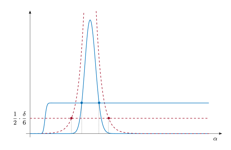
Figure 7: Graph of the left-hand and right-hand sides of (73) (solid blue lines) and of the curves that are used to obtain suitable lower and upper bounds to the solutions to (73) (dashed red lines).

The right-hand side, instead, for $k=0,\ldots,N-1$ takes value $0$ for both $\alpha=0$ and $\alpha=1$ and is first increasing and then decreasing, while for $k=N$ is $0$ for $\alpha=0$ only and it is increasing. A graphical illustration of the typical trend for the left-hand and right-hand sides of (73) for $\ln(3/\delta)<k\leq N-1$ is given in Figure 7 (solid blue lines). Given this state of things, it is clear that if the left-hand side of (73), call it $L(\alpha)$, is replaced by a function that lies below $L(\alpha)$, while the right-hand side, call it $R(\alpha)$, is replaced by a monotonically decreasing function that stays above $R(\alpha)$, the so-obtained equation has the property that any solution to it upper bounds the solution to (73) bigger than $k/N$, which in turn upper bounds $\overline{\varepsilon}_{k}$. Similarly, keeping the same replacement for the left-hand side of (73), but this time substituting the right-hand side $R(\alpha)$ with a monotonically increasing function that stays above $R(\alpha)$, an equation is obtained whose solutions provide lower-bounds to $\underline{\varepsilon}_{k}$. In the following, the sought upper bound to $\overline{\varepsilon}_{k}$ and lower bound to $\underline{\varepsilon}_{k}$ will be obtained by replacing $L(\alpha)$ with a suitable constant function and the right-hand side $R(\alpha)$ with a decreasing exponential and an increasing exponential function, respectively. See again Figure 7 for a graphical illustration (dashed red lines).

$\diamond$ Upper bound to $\overline{\varepsilon}_{k}$

Consider (73) for $k=0,1,\ldots,N-1$. Start with the left-hand side and notice that

$$\frac{\delta}{12}\leq\frac{\delta}{6}\left(1-\sum_{i=0}^{k}{4N+1\choose i}\alpha^{i}(1-\alpha)^{4N+1-i}\right)$$ (75)

for $\alpha\geq\frac{k+1}{4N+2}$. As a matter of fact, $\frac{k+1}{4N+2}$ is the mean of the Beta distribution having cumulative distribution function $1-\sum_{i=0}^{k}{4N+1\choose k}\alpha^{i}(1-\alpha)^{4N+1-i}$ and the mean of this Beta distribution is greater than its median, see Payton et al. (1989).
As for the right-hand side of (73), pick any number $c>1$ and notice that

$$\left(1+\frac{\delta}{6N}\right)N{N\choose k}\alpha^{k+1}(1-\alpha)^{N-k}$$

$$\leq \left(1+\frac{\delta}{6N}\right)(k+1){N+1\choose k+1}\alpha^{k+1}(1-\alpha)^{N+1-(k+1)}$$

$$\leq \frac{7}{6}(k+1)\sum_{i=0}^{k+1}{N+1\choose i}\alpha^{i}(1-\alpha)^{N+1-i}$$

$$\leq \frac{7}{6}(k+1)c^{k+1}\sum_{i=0}^{k+1}{N+1\choose i}\left(\frac{\alpha}{c}\right)^{i}(1-\alpha)^{N+1-i}$$

$$\leq \frac{7}{6}(k+1)c^{k+1}\sum_{i=0}^{N+1}{N+1\choose i}\left(\frac{\alpha}{c}\right)^{i}(1-\alpha)^{N+1-i}$$

$$= \frac{7}{6}(k+1)(1-(1-c))^{k+1}\left(1-\alpha\frac{c-1}{c}\right)^{N+1}$$

$$\leq \frac{7}{6}(k+1)\mathrm{e}^{-(1-c)(k+1)}\mathrm{e}^{-\alpha\frac{c-1}{c}(N+1)}$$

$$\leq \frac{7}{6}(k+1)\mathrm{e}^{-(1-c)(k+1)}\mathrm{e}^{-\alpha\frac{c-1}{c}N},$$

where the second-last inequality derives from relation $1-x\leq\mathrm{e}^{-x}$. Taking now

$$c=1+\frac{\sqrt{\ln(k+1)+\ln\frac{14}{\delta}}}{\sqrt{k+1}},$$

one obtains

$$\left(1+\frac{\delta}{6N}\right)N{N\choose k}\alpha^{k+1}(1-\alpha)^{N-k}$$ (76)

$$\leq \frac{7}{6}(k+1)\mathrm{e}^{\sqrt{\ln(k+1)+\ln\frac{14}{\delta}}\sqrt{k+1}}\mathrm{e}^{-\alpha\frac{\sqrt{\ln(k+1)+\ln\frac{14}{\delta}}\cdot N}{\sqrt{k+1}+\sqrt{\ln(k+1)+\ln\frac{14}{\delta}}}},$$

where the right-hand side is a monotonically decreasing function of $\alpha$. Using (75) and (76) together, in view of the argument given after (73) we have that the solution to

$$\frac{\delta}{12}=\frac{7}{6}(k+1)\mathrm{e}^{\sqrt{\ln(k+1)+\ln\frac{14}{\delta}}\sqrt{k+1}}\mathrm{e}^{-\alpha\frac{\sqrt{\ln(k+1)+\ln\frac{14}{\delta}}\cdot N}{\sqrt{k+1}+\sqrt{\ln(k+1)+\ln\frac{14}{\delta}}}}$$ (77)

upper bounds $\overline{\varepsilon}_{k}$ as long as the solution turns out to be no smaller than $\frac{k+1}{4N+2}$ (which is the condition to ensure that (75) is indeed true). Solving (77) for $\alpha$ gives

$$\overline{\alpha}=\frac{k+1}{N}+2\frac{\sqrt{k+1}\sqrt{\ln(k+1)+\ln\frac{14}{\delta}}}{N}+\frac{\ln(k+1)+\ln\frac{14}{\delta}}{N},$$

which is always greater than $\frac{k+1}{4N+2}$. Thus, it follows that, for $k=0,1,\ldots,N-1$,

$$\overline{\varepsilon}_{k}\leq\frac{k+1}{N}+2\frac{\sqrt{k+1}\sqrt{\ln(k+1)+\ln\frac{14}{\delta}}}{N}+\frac{\ln(k+1)+\ln\frac{14}{\delta}}{N}.$$

Moreover, the bound turns out to be valid for $k=N$ too, since $\overline{\varepsilon}_{N}=1$, while the right-hand side of the previous inequality is greater than $1$ for $k=N$. Using the fact that $\sqrt{\ln(k+1)+\ln\frac{14}{\delta}}\leq\sqrt{\ln(k+1)}+\sqrt{\ln(14)}+\sqrt{\ln\frac{1}{\delta}}$ in the previous expression, and re-arranging the terms, one obtains:

$$\overline{\varepsilon}_{k}\leq\frac{k}{N}+\frac{2\sqrt{k+1}\left(\sqrt{\ln(k+1)}+\sqrt{\ln(14)}\right)+\ln(k+1)+\ln(14)+1}{N}+2\frac{\sqrt{k+1}\sqrt{\ln\frac{1}{\delta}}}{N}+\frac{\ln\frac{1}{\delta}}{N}.$$

It is easy to verify that $\ln(k+1)+\ln(14)+1<4\sqrt{k+1}$; using this fact in the numerator of the second term together with $\sqrt{\ln(14)}+2<4$ yields

$$\overline{\varepsilon}_{k}\leq\frac{k}{N}+2\frac{\sqrt{k+1}}{N}\left(\sqrt{\ln(k+1)}+4\right)+2\frac{\sqrt{k+1}\sqrt{\ln\frac{1}{\delta}}}{N}+\frac{\ln\frac{1}{\delta}}{N},$$

which is the bound in (7).

$\diamond$ Lower bound to $\underline{\varepsilon}_{k}$

Consider (73) again, this time for $k>\ln(\frac{3}{\delta})$ as given in (74) (which, as we have seen, ensures that the solution lower than $k/N$ takes value in the interval $(0,1)$). The right-hand side of (73) is upper bounded as follows ($c$ is any number bigger than $1$):

$$\left(1+\frac{\delta}{6N}\right)N{N\choose k}\alpha^{k+1}(1-\alpha)^{N-k}$$

$$\leq \left(1+\frac{\delta}{6N}\right)(k+1){N+1\choose k+1}\alpha^{k+1}(1-\alpha)^{N+1-(k+1)}$$

$$\leq \frac{7}{6}(k+1)\sum_{i=k+1}^{N+1}{N+1\choose i}\alpha^{i}(1-\alpha)^{N+1-i}$$

$$\leq \frac{7}{6}(k+1)\frac{1}{c^{k+1}}\sum_{i=k+1}^{N+1}{N+1\choose i}(\alpha c)^{i}(1-\alpha)^{N+1-i}$$

$$\leq \frac{7}{6}(k+1)\frac{1}{c^{k+1}}\sum_{i=0}^{N+1}{N+1\choose i}(\alpha c)^{i}(1-\alpha)^{N+1-i}$$

$$= \frac{7}{6}(k+1)\frac{\big{(}1+\alpha(c-1)\big{)}^{N+1}}{\big{(}1+(c-1)\big{)}^{k+1}}$$

$$\leq \frac{7}{6}(k+1)\mathrm{e}^{\alpha(c-1)(N+1)}\mathrm{e}^{-\left(c-1-\frac{(c-1)^{2}}{2}\right)(k+1)},$$

where the last inequality derives from $\mathrm{e}^{x-\frac{x^{2}}{2}}\leq 1+x\leq\mathrm{e}^{x}$ for $x\geq 0$. With the choice

$$c=1+\frac{\sqrt{\ln(k+1)+\ln\frac{14}{\delta}}}{\sqrt{k+1}},$$

we now obtain

$$\left(1+\frac{\delta}{6N}\right)N{N\choose k}\alpha^{k+1}(1-\alpha)^{N-k}$$ (78)

$$\leq \frac{7}{6}(k+1)\mathrm{e}^{\alpha\frac{\sqrt{\ln(k+1)+\ln\frac{14}{\delta}}\cdot(N+1)}{\sqrt{k+1}}}\mathrm{e}^{-\sqrt{\ln(k+1)+\ln\frac{14}{\delta}}\sqrt{k+1}+\frac{1}{2}\left(\ln(k+1)+\ln\frac{14}{\delta}\right)},$$

where the right-hand side is an increasing function of $\alpha$. Using (75) and (78) together, in view of the argument given after (73) we have that the solution to

$$\frac{\delta}{12}=\frac{7}{6}(k+1)\mathrm{e}^{\alpha\frac{\sqrt{\ln(k+1)+\ln\frac{14}{\delta}}\cdot(N+1)}{\sqrt{k+1}}}\mathrm{e}^{-\sqrt{\ln(k+1)+\ln\frac{14}{\delta}}\sqrt{k+1}+\frac{1}{2}\left(\ln(k+1)+\ln\frac{14}{\delta}\right)}$$ (79)

lower bounds $\underline{\varepsilon}_{k}$ as long as the solution turns out to be no smaller than $\frac{k+1}{4N+2}$ (which is the condition to ensure that (75) is indeed true). Solving (79) for $\alpha$ gives

$$\underline{\alpha}=\frac{k+1}{N+1}-\frac{3}{2}\frac{\sqrt{k+1}}{N+1}\sqrt{\ln(k+1)+\ln\frac{14}{\delta}}.$$ (80)

Hence, for those $k$ for which $\underline{\alpha}\geq\frac{k+1}{4N+2}$, we have that $\underline{\varepsilon}_{k}\geq\underline{\alpha}$, which also clearly gives the looser inequality

$$\underline{\varepsilon}_{k}\geq\frac{k+1}{N+1}-3\frac{\sqrt{k+1}}{N+1}\sqrt{\ln(k+1)+\ln\frac{14}{\delta}}.$$ (81)

On the other hand, if $k$ is such that $\underline{\alpha}<\frac{k+1}{4N+2}$, then, substituting the expression for $\underline{\alpha}$ given in (80) in relation $\underline{\alpha}<\frac{k+1}{4N+2}$ yields

$$\frac{3}{2}\frac{\sqrt{k+1}}{N+1}\sqrt{\ln(k+1)+\ln\frac{14}{\delta}}>\frac{k+1}{N+1}-\frac{k+1}{4N+2}>\frac{1}{2}\cdot\frac{k+1}{N+1},$$

from which

$$\frac{k+1}{N+1}-3\frac{\sqrt{k+1}}{N+1}\sqrt{\ln(k+1)+\ln\frac{14}{\delta}}<0,$$

and, since $\underline{\varepsilon}_{k}\geq 0$ by definition, we conclude that (81) remains valid in this case as well.

Go now back to re-consider condition $k>\ln(\frac{3}{\delta})$ introduced at the beginning of this part about lower bounding $\underline{\varepsilon}_{k}$, and consider the opposite case that $k\leq\ln(\frac{3}{\delta})$. If so, it also holds that $k+1\leq 3\sqrt{k+1}\sqrt{\ln(k+1)+\ln\frac{14}{\delta}}$, which in turn implies that the right-hand side of (81) is no bigger than $0$. This, in view of relation $\underline{\varepsilon}_{k}\geq 0$, proves that (81) is valid in this case as well. Hence, we conclude that (81) is valid for all $k=0,1,\ldots,N$. Since $\frac{k+1}{N+1}\geq\frac{k}{N}$, $\frac{1}{N+1}<\frac{1}{N}$, and $\sqrt{\ln(k+1)+\ln\frac{14}{\delta}}\leq\sqrt{\ln(k+1)}+\sqrt{\ln(14)}+\sqrt{\ln\frac{1}{\delta}}$, from (81) we also obtain

$$\underline{\varepsilon}_{k}\geq\frac{k}{N}-3\frac{\sqrt{k+1}}{N}\left(\sqrt{\ln(k+1)}+\sqrt{\ln(14)}\right)-3\frac{\sqrt{k+1}\sqrt{\ln\frac{1}{\delta}}}{N}.$$

The bound in (8) is finally obtained by noticing that $\sqrt{\ln(14)}<2$.

This concludes the proof. $\star$

Acknowledgments and Disclosure of Funding

The authors would like to thank professor Nicolò Cesa-Bianchi for insightful and inspiring discussions on various parts of this manuscript. They also express their gratitude to the editor and to anonimous reviewers for generously providing comments that helped improve the paper.

The research presented in this article has been partly supported by MUR under the PRIN 2022 project “The Scenario Approach for Control and Non-Convex Design” (project number D53D23001440006) and by FAIR (Future Artificial Intelligence Research) project, funded by the NextGenerationEU program within the PNRR-PE-AI scheme (M4C2, Investment 1.3, Line on Artificial Intelligence).

Appendix A A study of the graph of $\tilde{\Psi}_{k,\delta}$

For $k=0,1,\ldots,N-1$, the derivative of $\tilde{\Psi}_{k,\delta}$, i.e.,

$$\frac{\mathrm{d}\tilde{\Psi}_{k,\delta}}{\mathrm{d}\alpha}(\alpha)=\frac{\delta}{2N}\sum_{m=k}^{N-1}\frac{{m\choose k}}{{N\choose k}}(N-m)(1-\alpha)^{-(N-m+1)}-\frac{\delta}{6N}\sum_{m=N+1}^{4N}\frac{{m\choose k}}{{N\choose k}}(m-N)(1-\alpha)^{m-N-1},$$

is a strictly increasing function with limit $-\infty$ for $\alpha\to-\infty$ and limit $+\infty$ for $\alpha\to 1$. Hence, over the interval $(-\infty,1)$, $\tilde{\Psi}_{k,\delta}$ is first decreasing and then increasing, with a unique minimum. Since $\tilde{\Psi}_{k,\delta}\to+\infty$ for both $\alpha\to-\infty$ and $\alpha\to 1$, to prove that the equation $\tilde{\Psi}_{k,\delta}(\alpha)=1$ has indeed two solutions, it is enough to exhibit an $\bar{\alpha}\in(-\infty,1)$ for which $\tilde{\Psi}_{k,\delta}(\bar{\alpha})<1$. To this aim, consider $\bar{\alpha}=\frac{k}{N}$ and notice that

$$\tilde{\Psi}_{k,\delta}(k/N)=\frac{\delta}{2}\left[\frac{1}{N}\sum_{m=k}^{N-1}\frac{{m\choose k}}{{N\choose k}}\frac{N^{N-m}}{(N-k)^{N-m}}+\frac{1}{3N}\sum_{m=N+1}^{4N}\frac{{m\choose k}}{{N\choose k}}\frac{(N-k)^{m-N}}{N^{m-N}}\right].$$ (82)

For $m=k,\ldots,N-1$, we have

$$\frac{{m\choose k}}{{N\choose k}}\frac{N^{N-m}}{(N-k)^{N-m}}=\prod_{i=0}^{N-m-1}\left(\frac{N-k-i}{N-i}\cdot\frac{N}{N-k}\right)\leq 1,$$

where the inequality is satisfied since each term $\frac{N-k-i}{N-i}\cdot\frac{N}{N-k}$ in the product is no bigger than $1$. Similarly, for $m=N+1,\ldots,4N$ we have

$$\frac{{m\choose k}}{{N\choose k}}\frac{(N-k)^{m-N}}{N^{m-N}}=\prod_{i=1}^{m-N}\left(\frac{N+i}{N-k+i}\cdot\frac{N-k}{N}\right)\leq 1$$

(again it is straightforward to verify that each term $\frac{N+i}{N-k+i}\cdot\frac{N-k}{N}$ is no bigger than $1$). We therefore see that both sums in the square brackets in the right-hand side of (82) are arithmetic means of quantities no bigger than $1$, and therefore they are no bigger than $1$ as well. This gives $\tilde{\Psi}_{k,\delta}(k/N)\leq\delta<1$, and it also shows that $\underline{\alpha}_{k}<\frac{k}{N}<\overline{\alpha}_{k}$.

Appendix B MATLAB code

In this Appendix, we provide efficient bisection algorithms in the MATLAB computing environment for the evaluation of $\varepsilon_{k}$, $\underline{\varepsilon}_{k}$ and $\overline{\varepsilon}_{k}$. The algorithms take advantage of some reformulations of the equations $\Psi_{k,\delta}(\alpha)=1$ and $\tilde{\Psi}_{k,\delta}(\alpha)=1$ as discussed in the beginning of the proof of Proposition 8 in Section 5.4. A summary of these reformulations are provided before the MATLAB codes.

B.1 Bisection algorithm for the computation of $\varepsilon_{k}$

Equation $\Psi_{k,\delta}(\alpha)=1$ for $k=0,\ldots,N-1$ can be rewritten as

$$\frac{\delta}{N}\sum_{m=k}^{N-1}{m\choose k}(1-\alpha)^{m-k}={N\choose k}(1-\alpha)^{N-k},$$

and, using a formula analogous to (72) in Section 5.4, but with $N-1$ in place of $4N$, this equation is shown to be equivalent over the interval $(0,1)$ to

$$\delta\left(1-\sum_{i=0}^{k}{N\choose k}\alpha^{i}(1-\alpha)^{N-i}\right)=\alpha N{N\choose k}\alpha^{k}(1-\alpha)^{N-k}.$$

The only solution to this equation in $(0,1)$ is $\varepsilon_{k}$ and it can be computed by bisection starting from $0$ and $1$ as initial extremes. Apart from the coefficient $\delta$, the left-hand side is an incomplete Beta function with parameters $k+1$ and $N-k$, which can be efficiently and accurately evaluated with the betainc function of MATLAB. Similarly, apart from the term $\alpha N$, the right-hand side can be computed as the difference of two incomplete beta functions. The following code provides a ready-to-use implementation of the bisection algorithm in the MATLAB environment.

function eps = find_eps(k,N,delta)

if k==N
eps = 1;
else
t1 = 0;
t2 = 1;
while t2-t1 > 1e-10
t = (t1+t2)/2;
left = delta*betainc(t,k+1,N-k);
right = t*N*(betainc(t,k,N-k+1)-betainc(t,k+1,N-k));
if left > right
t2=t;
else
t1=t;
end
end
eps = t2;
end

end

B.2 Bisection algorithm for the computation of $\underline{\varepsilon}_{k}$ and $\overline{\varepsilon}_{k}$

Following the same argument given in the proof of Proposition 8 to derive (71) (see Section 5.4), it is easy to see that equation $\tilde{\Psi}_{k,\delta}(\alpha)=1$ can be reformulated as

$$\frac{\delta}{3N}\sum_{m=k}^{N-1}{m\choose k}(1-\alpha)^{m-k}+\frac{\delta}{6N}\sum_{m=k}^{4N}{m\choose k}(1-\alpha)^{m-k}=\left(1+\frac{\delta}{6N}\right){N\choose k}(1-\alpha)^{N-k}.$$

Using again formula (72) for the second term in the left-hand side and its variant with $N-1$ in place of $4N$ for the first term, one obtains that $\tilde{\Psi}_{k,\delta}(\alpha)=1$ is equivalent over the interval $(0,1)$ to the equation

$$\frac{\delta}{3}\left(1-\sum_{i=0}^{k}{N\choose k}\alpha^{i}(1-\alpha)^{N-i}\right)+\frac{\delta}{6}\left(1-\sum_{i=0}^{k}{4N+1\choose k}\alpha^{i}(1-\alpha)^{4N+1-i}\right)$$

$$\quad=\left(1+\frac{\delta}{6N}\right)\alpha N{N\choose k}\alpha^{k}(1-\alpha)^{N-k},$$

where, again, the left- and the right-hand sides can be conveniently computed via the incomplete Beta function. A bisection algorithm with $\frac{k}{N}$ and $1$ as extremes can be used to compute $\overline{\alpha}_{k}=\overline{\varepsilon}_{k}$ for $k=0,\ldots,N-1$; instead, for $k=0,\ldots,N$, using $0$ and $\frac{k}{N}$ as extremes, the bisection algorithm converges to $\underline{\alpha}_{k}=\underline{\varepsilon}_{k}$ when $\underline{\alpha}_{k}>0$ and to $0=\underline{\varepsilon}_{k}$ when $\underline{\alpha}_{k}\leq 0$. The following code provides an implementation in MATLAB.

function [epsL, epsU] = find_epsLU(k,N,delta)

t1 = 0;
t2 = k/N;
while t2-t1 > 1e-10
t = (t1+t2)/2;
left = delta/3*betainc(t,k+1,N-k)+delta/6*betainc(t,k+1,4*N+1-k);
right = (1+delta/6/N)*t*N*(betainc(t,k,N-k+1)-betainc(t,k+1,N-k));
if left > right
t1=t;
else
t2=t;
end
end
epsL = t1;

if k==N
epsU = 1;
else
t1 = k/N;
t2 = 1;
while t2-t1 > 1e-10
t = (t1+t2)/2;
left = (delta/2-delta/6)*betainc(t,k+1,N-k)+delta/6*betainc(t,k+1,4*N+1-k);
right = (1+delta/6/N)*t*N*(betainc(t,k,N-k+1)-betainc(t,k+1,N-k));
if left > right
t2=t;
else
t1=t;
end
end
epsU = t2;
end

end

Appendix C Proof of (B) in (36)

Let $\tau>0$ be a number smaller than $1-\varepsilon_{k}$ for all $k$’s for which $\varepsilon_{k}\neq 1$. Matters of convenience (as shown later) suggest to introduce a modified Lagrangian that corresponds to a continuous cost function as follows

$$\mathfrak{L}_{\tau} = \sum_{k=0}^{N}{N\choose k}\int_{[0,1]}\varphi_{k,\tau}(\alpha)\;\mathrm{d}\mathfrak{m}^{+}_{k,N}-\sum_{m=0}^{M}\lambda_{m}\left(\sum_{k=0}^{m}{m\choose k}\int_{[0,1]}\mathrm{d}\mathfrak{m}^{+}_{k,m}-1\right)$$

$$-\sum_{m=0}^{M-1}\sum_{k=0}^{m}\int_{[0,1]}\mu^{+}_{k,m}(\alpha)\;\mathrm{d}\!\left[\mathfrak{m}^{+}_{k,m+1}-(1-\alpha)\mathfrak{m}^{+}_{k,m}\right],$$

where: for all $k$ for which $\varepsilon_{k}\neq 1$, $\varphi_{k,\tau}(\alpha)$ is a continuous function equal to $0$ for $\alpha\in[0,\varepsilon_{k}-\tau]$, equal to $1$ for $\alpha\in[\varepsilon_{k},1]$, and with a linear slope connecting $0$ to $1$ in between; while $\varphi_{k,\tau}(\alpha)$ is identically zero when $\varepsilon_{k}=1$. We show below the validity of the following relations:

$$\begin{array}[]{ccc}\sup_{\{\mathfrak{m}^{+}_{k,m}\}}\inf_{\begin{subarray}{c}\{\lambda_{m}\}\\ \{\mu^{+}_{k,m}\}\end{subarray}}\mathfrak{L}_{\tau}&=&\inf_{\begin{subarray}{c}\{\lambda_{m}\}\\ \{\mu^{+}_{k,m}\}\end{subarray}}\sup_{\{\mathfrak{m}^{+}_{k,m}\}}\mathfrak{L}_{\tau}\\ \downarrow_{\tau\downarrow 0}&&\mathbin{\rotatebox[origin={c}]{90.0}{$\displaystyle\leq$}}\\ \sup_{\{\mathfrak{m}^{+}_{k,m}\}}\inf_{\begin{subarray}{c}\{\lambda_{m}\}\\ \{\mu^{+}_{k,m}\}\end{subarray}}\mathfrak{L}&\leq&\inf_{\begin{subarray}{c}\{\lambda_{m}\}\\ \{\mu^{+}_{k,m}\}\end{subarray}}\sup_{\{\mathfrak{m}^{+}_{k,m}\}}\mathfrak{L}.\end{array}$$ (83)

Notice that the above relations imply the sought result that

$$\sup_{\{\mathfrak{m}^{+}_{k,m}\}}\inf_{\begin{subarray}{c}\{\lambda_{m}\}\\ \{\mu^{+}_{k,m}\}\end{subarray}}\mathfrak{L}=\inf_{\begin{subarray}{c}\{\lambda_{m}\}\\ \{\mu^{+}_{k,m}\}\end{subarray}}\sup_{\{\mathfrak{m}^{+}_{k,m}\}}\mathfrak{L}$$

because

$$\inf_{\begin{subarray}{c}\{\lambda_{m}\}\\ \{\mu^{+}_{k,m}\}\end{subarray}}\sup_{\{\mathfrak{m}^{+}_{k,m}\}}\mathfrak{L}$$

is in sandwich between

$$\sup_{\{\mathfrak{m}^{+}_{k,m}\}}\inf_{\begin{subarray}{c}\{\lambda_{m}\}\\ \{\mu^{+}_{k,m}\}\end{subarray}}\mathfrak{L}$$

and

$$\inf_{\begin{subarray}{c}\{\lambda_{m}\}\\ \{\mu^{+}_{k,m}\}\end{subarray}}\sup_{\{\mathfrak{m}^{+}_{k,m}\}}\mathfrak{L}_{\tau},$$

two quantities that converge one onto the other as $\tau\downarrow 0$.

The two inequalities in (83) are justified as follows: the $\leq$ at the bottom of (83) is valid because relation “$\sup\inf\leq\inf\sup$” is always true, while the $\mathbin{\rotatebox[origin={c}]{90.0}{$\leq$}}$ on the right follows from the fact that $\varphi_{k,\tau}(\alpha)$ in $\mathfrak{L}_{\tau}$ is greater than or equal to $\mathbbm{1}_{\alpha\in(\varepsilon_{k},1]}$ in $\mathfrak{L}$.

What remains to show is thus the $=$ at the top of (83) and the convergence $\downarrow_{\tau\downarrow 0}$ on the left.

We first show that

$$\sup_{\{\mathfrak{m}^{+}_{k,m}\}}\inf_{\begin{subarray}{c}\{\lambda_{m}\}\\ \{\mu^{+}_{k,m}\}\end{subarray}}\mathfrak{L}_{\tau}=\inf_{\begin{subarray}{c}\{\lambda_{m}\}\\ \{\mu^{+}_{k,m}\}\end{subarray}}\sup_{\{\mathfrak{m}^{+}_{k,m}\}}\mathfrak{L}_{\tau},$$ (84)

for which purpose we need to introduce a proper topological vector space, Rudin (1991), as specified in the following.

• Consider the vector space $\mathcal{M}$ of finite signed measures $\mathfrak{m}$ with support on $[0,1]$. Moreover, let $\mathcal{LF}$ be the vector space of linear functionals on $\mathcal{M}$ of the form $\int_{[0,1]}\mu(\alpha)\;\mathrm{d}\mathfrak{m}$, where $\mu$ is a continuous function ($\mu\in\textsf{C}^{0}[0,1]$). In $\mathcal{M}$, introduce the weak topology induced by $\mathcal{LF}$, see Section 3.8 in Rudin (1991). This weak topology makes $\mathcal{M}$ into a locally convex topological vector space whose dual space coincides with $\mathcal{LF}$, see Theorem 3.10 in Rudin (1991). By also considering the standard topology of $\mathbb{R}$ generated by open intervals, the ambient space in which we are going to work is the topological vector space given by $\mathbb{R}\times\mathbb{R}^{M+1}\times\mathcal{M}^{\frac{(M+1)M}{2}}=:\mathcal{S}$ equipped with the product topology.
  
  The interpretation of $\mathcal{S}$ is that it is the codomain of an operator that maps $\mathfrak{m}^{+}_{k,m}$, $m=0,1,\ldots,M$, $k=,0,\ldots,m$ into an element of $\mathcal{S}$ according to the rule:

  $$\big{\{}\mathfrak{m}^{+}_{k,m}\big{\}}_{\begin{subarray}{l}m=0,1,\ldots,M\\ k=0,\ldots,m\end{subarray}} \to \left\{\begin{array}[]{ll}\sum_{k=0}^{N}{N\choose k}\int_{[0,1]}\varphi_{k,\tau}(\alpha)\ \mathrm{d}\mathfrak{m}^{+}_{k,N}&\quad(\in\mathbb{R})\\ \left\{\sum_{k=0}^{m}{m\choose k}\int_{[0,1]}\mathrm{d}\mathfrak{m}^{+}_{k,m}-1\right\}_{m=0,1,\ldots,M}&\quad(\in\mathbb{R}^{M+1})\\ \big{\{}\mathfrak{m}^{+}_{k,m+1}-(1-\alpha)\;\mathfrak{m}^{+}_{k,m}\big{\}}_{\begin{subarray}{l}m=0,1,\ldots,M-1\\ k=0,\ldots,m\end{subarray}}&\quad(\in\mathcal{M}^{\frac{(M+1)M}{2}})\end{array}\right.$$

  (note that this operator returns various terms that are found in $\mathfrak{L}_{\tau}$). We next consider the image of this operator, that is, the range of points in $\mathcal{S}$ that are reached as $\{\mathfrak{m}^{+}_{k,m}\}$ varies in its domain $\left(\mathcal{M}^{+}\right)^{\frac{(M+2)(M+1)}{2}}$. To this image, we further add an arbitrary positive measure $\mathfrak{p}^{+}_{k,m}$ to each term $\mathfrak{m}^{+}_{k,m+1}-(1-\alpha)\;\mathfrak{m}^{+}_{k,m}$ (the reason for this will become clear shortly). The final set that is obtained as $\{\mathfrak{m}^{+}_{k,m}\}$ and $\{\mathfrak{p}^{+}_{k,m}\}$ vary over their domains is denoted by $H$:

  $$H := \Big{\{}(v,\{r_{m}\},\big{\{}\mathfrak{q}_{k,m}\big{\}})\in\mathbb{R}\times\mathbb{R}^{M+1}\times\mathcal{M}^{\frac{(M+1)M}{2}}:$$ (86)

  $$\quad\quad\quad v=\sum_{k=0}^{N}{N\choose k}\int_{[0,1]}\varphi_{k,\tau}(\alpha)\ \mathrm{d}\mathfrak{m}^{+}_{k,N},$$

  $$\quad\quad\quad\{r_{m}\}=\left\{\sum_{k=0}^{m}{m\choose k}\int_{[0,1]}\mathrm{d}\mathfrak{m}^{+}_{k,m}-1\right\},$$

  $$\quad\quad\quad\big{\{}\mathfrak{q}_{k,m}\big{\}}=\big{\{}\mathfrak{m}^{+}_{k,m+1}-(1-\alpha)\;\mathfrak{m}^{+}_{k,m}+\mathfrak{p}^{+}_{k,m}\big{\}},$$

  $$\quad\mbox{where, for all }m\mbox{ and }k,\ \ \mathfrak{m}^{+}_{k,m}\in\mathcal{M}^{+},\mathfrak{p}^{+}_{k,m}\in\mathcal{M}^{+}\Big{\}}.$$

  The closure of $H$ in the topology of $\mathcal{S}$ is denoted by $\bar{H}$. The following definitions refer to the restrictions of $H$ and $\bar{H}$ to the line where all $r_{m}$ and $\mathfrak{q}_{k,m}$ are set to $0$ (i.e., the zero element in $\mathbb{R}$ and $\mathcal{M}$, respectively): quantities

  $$V := \sup\Big{\{}v:\;(v,\{r_{m}=0\},\big{\{}\mathfrak{q}_{k,m}=0\big{\}})\in H\Big{\}}$$

  $$\bar{V} := \sup\Big{\{}v:\;(v,\{r_{m}=0\},\big{\{}\mathfrak{q}_{k,m}=0\big{\}})\in\bar{H}\Big{\}}$$

  are called value and supervalue, respectively. With this notation, we have

  $$\sup_{\{\mathfrak{m}^{+}_{k,m}\}}\inf_{\begin{subarray}{c}\{\lambda_{m}\}\\ \{\mu^{+}_{k,m}\}\end{subarray}}\mathfrak{L}_{\tau}=V$$

  (this fact easily follows from an argument similar to the proof of equality (A) in (36) after noting that $V$ in the present context plays the same role as $\gamma_{M}$ in left-hand side of(36)). On the other hand, we also have

  $$\inf_{\begin{subarray}{c}\{\lambda_{m}\}\\ \{\mu^{+}_{k,m}\}\end{subarray}}\sup_{\{\mathfrak{m}^{+}_{k,m}\}}\mathfrak{L}_{\tau}=\bar{V},$$ (87)

  which requires the proof given below, based on Hahn-Banach theorem. After showing this, the proof of (84) is concluded by proving that $V=\bar{V}$.

  • To prove (87), note that $\bar{H}$ is convex and closed and, for any $\varepsilon>0$, point $s^{\varepsilon}:=(\bar{V}+\varepsilon,\{r_{m}=0\},\{\mathfrak{q}_{k,m}=0\})\notin\bar{H}$. By an application of Hahn-Banach theorem (see Theorem 3.4 in Rudin, 1991), one can therefore find a linear continuous functional defined over $\mathcal{S}$ that “separates” $\bar{H}$ from $s^{\varepsilon}$ in such a way that the functional computed at any point of $\bar{H}$ is strictly smaller than the functional computed at $s^{\varepsilon}$.

    A generic linear continuous functional defined over $\mathcal{S}$ is written as

    $$a\cdot v-\sum_{m=0}^{M}\lambda_{m}r_{m}-\sum_{m=0}^{M-1}\sum_{k=0}^{m}\int_{[0,1]}\mu_{k,m}(\alpha)\;\mathrm{d}\mathfrak{q}_{k,m},$$ (88)

    where $a,\lambda_{m}\in\mathbb{R}$ and $\mu_{k,m}\in\textsf{C}^{0}[0,1]$, and hence the separation condition yields

    $$\begin{array}[]{r}a^{\varepsilon}\cdot v-\sum_{m=0}^{M}\lambda_{m}^{\varepsilon}r_{m}-\sum_{m=0}^{M-1}\sum_{k=0}^{m}\int_{[0,1]}\mu_{k,m}^{\varepsilon}(\alpha)\;\mathrm{d}\mathfrak{q}_{k,m}<a^{\varepsilon}\cdot(\bar{V}+\varepsilon),\\ \forall(v,\{r_{m}\},\{\mathfrak{q}_{k,m}\})\in\bar{H},\end{array}$$ (89)

    where $a^{\varepsilon},\lambda_{m}^{\varepsilon},\mu_{k,m}^{\varepsilon}(\alpha)$ are specific choices of $a,\lambda_{m},\mu_{k,m}(\alpha)$ in (88). Specializing (89) to a point in $\bar{H}$ with $\{r_{m}=0\}$ and $\{\mathfrak{q}_{k,m}=0\}$ yields $a^{\varepsilon}\cdot v<a^{\varepsilon}\cdot(\bar{V}+\varepsilon)$, which implies $a^{\varepsilon}>0$. Moreover, noting that $\mathfrak{q}_{k,m}$ contains $\mathfrak{p}^{+}_{k,m}$, which is positive and arbitrarily large, one concludes that $\mu_{k,m}^{\varepsilon}$ must be non-negative for the inequality to hold over the whole $\bar{H}$. To take notice of this fact, in subsequent derivations we write $\mu_{k,m}^{\varepsilon,+}$ in place of $\mu_{k,m}^{\varepsilon}$. Dividing by $a^{\varepsilon}$, inequality (89) now gives

    $$v-\sum_{m=0}^{M}\frac{\lambda_{m}^{\varepsilon}}{a^{\varepsilon}}r_{m}-\sum_{m=0}^{M-1}\sum_{k=0}^{m}\int_{[0,1]}\frac{\mu_{k,m}^{\varepsilon,+}(\alpha)}{a^{\varepsilon}}\;\mathrm{d}\mathfrak{q}_{k,m}<\bar{V}+\varepsilon,\ \ \ \forall(v,\{r_{m}\},\{\mathfrak{q}_{k,m}\})\in\bar{H}.$$

    Given the arbitrariness of $\varepsilon$ and restricting attention to $H\subseteq\bar{H}$, one concludes that

    $$\inf_{\begin{subarray}{c}\{\lambda_{m}\}\\ \{\mu^{+}_{k,m}\}\end{subarray}}\sup_{(v,\{r_{m}\},\{\mathfrak{q}_{k,m}\})\in H}\;\left\{v-\sum_{m=0}^{M}\lambda_{m}r_{m}-\sum_{m=0}^{M-1}\sum_{k=0}^{m}\int_{[0,1]}\mu_{k,m}^{+}(\alpha)\;\mathrm{d}\mathfrak{q}_{k,m}\right\}\leq\bar{V}.$$ (90)

    On the other hand, recalling the expression of $v$, $r_{m}$, $\mathfrak{q}_{k,m}$ in the definition of $H$ given in (86), the left-hand side of (90) can be rewritten as

    $$\inf_{\begin{subarray}{c}\{\lambda_{m}\}\\ \{\mu^{+}_{k,m}\}\end{subarray}}\sup_{\{\mathfrak{m}^{+}_{k,m}\},\{\mathfrak{p}^{+}_{k,m}\}}\;\left\{\mathfrak{L}_{\tau}-\sum_{m=0}^{M-1}\sum_{k=0}^{m}\int_{[0,1]}\mu_{k,m}^{+}(\alpha)\;\mathrm{d}\mathfrak{p}^{+}_{k,m}\right\},$$

    which further becomes

    $$\inf_{\begin{subarray}{c}\{\lambda_{m}\}\\ \{\mu^{+}_{k,m}\}\end{subarray}}\left\{\sup_{\{\mathfrak{m}^{+}_{k,m}\}}\;\mathfrak{L}_{\tau}+\sup_{\{\mathfrak{p}^{+}_{k,m}\}}\left\{-\sum_{m=0}^{M-1}\sum_{k=0}^{m}\int_{[0,1]}\mu_{k,m}^{+}(\alpha)\;\mathrm{d}\mathfrak{p}^{+}_{k,m}\right\}\right\}=\inf_{\begin{subarray}{c}\{\lambda_{m}\}\\ \{\mu^{+}_{k,m}\}\end{subarray}}\sup_{\{\mathfrak{m}^{+}_{k,m}\}}\mathfrak{L}_{\tau},$$ (91)

    where in the last equality the second term has been suppressed because $\sup_{\{\mathfrak{p}^{+}_{k,m}\}}$ is taken over non-positive quantities and $\mathfrak{p}^{+}_{k,m}=0$ is admissible. Altogether, (90) and (91) give the relation

    $$\inf_{\begin{subarray}{c}\{\lambda_{m}\}\\ \{\mu^{+}_{k,m}\}\end{subarray}}\sup_{\{\mathfrak{m}^{+}_{k,m}\}}\;\mathfrak{L}_{\tau}\leq\bar{V}.$$ (92)

    To prove (87), we show that strict inequality in (92) cannot hold. Indeed, in the opposite, there would exist a linear continuous functional of the form (88) that separates $H$ from $\bar{P}:=(\bar{V},\{r_{m}=0\},\{\mathfrak{q}_{k,m}=0\})$. If we now consider the open set $A$ obtained as counter-image of the reals greater than the value taken by this functional at $\bar{P}$ minus a small enough margin, then $A$ contains $\bar{P}$, while $A$ leaves out all $H$, contradicting the fact that $\bar{P}$ is a contact point of $H$.

  We now show that $V=\bar{V}$, so closing the proof of (84). We start by constructing a sequence of neighborhoods of $\bar{P}=(\bar{V},\{r_{m}=0\},\{\mathfrak{q}_{k,m}=0\})$ that exhibit asymptotic properties of interest. Consider a countable set of continuous functions $g_{1},g_{2},\ldots$ dense in $\textsf{C}^{0}[0,1]$ with respect to the $\sup$ norm (e.g., polynomials with rational coefficients, see Theorem 7.26 in Rudin, 1976). For $i=1,2,\ldots$, the neighborhoods of $\bar{P}$ are defined as follows:

  $$O_{i} := \Big{\{}(v,\{r_{m}\},\{\mathfrak{q}_{k,m}\})\mbox{ with }|v-\bar{V}|<1/i;\ |r_{m}|<1/i,m=0,1,\ldots,M;\mbox{ and }$$

  $$\max_{j=1,\ldots,i}\left|\int_{[0,1]}g_{j}(\alpha)\;\mathrm{d}\mathfrak{q}_{k,m}\right|<1/i,m=0,1,\ldots,M-1\mbox{ and }k=0,\ldots,m\Big{\}}.$$

  Further, for any $m=0,1,\ldots,M$ and $k=0,1,\ldots,m$ consider sequences $\mathfrak{m}^{+,i}_{k,m}$ and $\mathfrak{p}^{+,i}_{k,m}$ indexed in $i$ such that, for each $i=1,2,\ldots$, the pair $(\{\mathfrak{m}^{+,i}_{k,m}\},\{\mathfrak{p}^{+,i}_{k,m}\})$ maps into a point of $H$ that is also in $O_{i}$ (such sequences certainly exist since $\bar{P}$ is a contact point of $H$, see Footnote 37). For these sequences we have

  $$\lim_{i\to\infty}\sum_{k=0}^{N}{N\choose k}\int_{[0,1]}\varphi_{k,\tau}(\alpha)\;\mathrm{d}\mathfrak{m}^{+,i}_{k,N}=\bar{V};$$ (93)

  $$\lim_{i\to\infty}\left[\sum_{k=0}^{m}{m\choose k}\int_{[0,1]}\mathrm{d}\mathfrak{m}^{+,i}_{k,m}-1\right]=0,\ \ \ m=0,1,\ldots,M;$$ (94)

  $$\lim_{i\to\infty}\int_{[0,1]}g_{j}(\alpha)\;\mathrm{d}[\mathfrak{m}^{+,i}_{k,m+1}-(1-\alpha)\;\mathfrak{m}^{+,i}_{k,m}+\mathfrak{p}^{+,i}_{k,m}]=0,$$

  $$\quad\forall g_{j}(\alpha),\;j=1,2,\ldots,\ \ \ m=0,1,\ldots,M-1,\ \ \ k=0,\ldots,m.$$ (95)

  In view of (94), for a given $m$ and $k$, measures $\mathfrak{m}^{+,i}_{k,m}$ are uniformly bounded in $i$ (i.e., $\mathfrak{m}^{+,i}_{k,m}([0,1])\leq C$, $\forall i$, for some positive constant $C<+\infty$). Since measures $\mathfrak{m}^{+,i}_{k,m}$ are supported in $[0,1]$, by Prokhorov’s theorem (see Shiryaev, 1996, Theorem 1, Section 2, Chapter III), we then conclude that there exists a sub-sequence of indexes $i_{h}$ such that $\mathfrak{m}^{+,i_{h}}_{k,m}$ has weak limit $\bar{\mathfrak{m}}^{+}_{k,m}\in\mathcal{M}^{+}$. By repeating the same reasoning in a nested manner, we can further find a sub-sequence of the indexes $i_{h}$ such that weak convergence holds for a new choice of $m$ and $k$. Proceeding the same way for all choices of $m$ and $k$, we conclude that there exists a sub-sequence of indexes (which, with a little abuse of notation, we still indicate as $i_{h}$) for which

  $$\int_{[0,1]}f(\alpha)\;\mathrm{d}\bar{\mathfrak{m}}^{+}_{k,m}=\lim_{i_{h}\to\infty}\int_{[0,1]}f(\alpha)\;\mathrm{d}\mathfrak{m}^{+,i_{h}}_{k,m},\quad\forall\;m,k,$$ (96)

  holds for any continuous function $f\in\textsf{C}^{0}[0,1]$.
  
  Since $\varphi_{k,\tau}$, as well as the constant function equal to $1$, are continuous, (96) together with (93) and (94) yield

  $$\sum_{k=0}^{N}{N\choose k}\int_{[0,1]}\varphi_{k,\tau}(\alpha)\;\mathrm{d}\bar{\mathfrak{m}}^{+}_{k,N}=\bar{V}$$ (97)

  and

  $$\sum_{k=0}^{m}{m\choose k}\int_{[0,1]}\mathrm{d}\bar{\mathfrak{m}}^{+}_{k,m}-1=0,\quad m=0,1,\ldots,M.$$ (98)

  Turn now to consider (95), from which we have

  $$\lim_{i_{h}\to\infty}\int_{[0,1]}g_{j}(\alpha)\;\mathrm{d}[\mathfrak{m}^{+,i_{h}}_{k,m+1}-(1-\alpha)\;\mathfrak{m}^{+,i_{h}}_{k,m}]=-\lim_{i_{h}\to\infty}\int_{[0,1]}g_{j}(\alpha)\;\mathrm{d}\mathfrak{p}^{+,i_{h}}_{k,m},$$ (99)

  where the limit in (95) restricted to the sub-sequence $i_{h}$ can be broken up in the two limits in (99) because the left-hand side of (99) exists due to the weak convergence of measures $\mathfrak{m}^{+,i_{h}}_{k,m}$ (note that $g_{j}(\alpha)$ and $g_{j}(\alpha)(1-\alpha)$ are continuous functions). For the functions $g_{j}$ that are non-negative (i.e., $g_{j}(\alpha)\geq 0$, $\forall\alpha$), which we henceforth write as $g^{+}_{j}$ to help interpretation, (99) gives

  $$\lim_{i_{h}\to\infty}\int_{[0,1]}g^{+}_{j}(\alpha)\;\mathrm{d}[\mathfrak{m}^{+,i_{h}}_{k,m+1}-(1-\alpha)\;\mathfrak{m}^{+,i_{h}}_{k,m}]\leq 0.$$ (100)

  Taking now any non-negative function $f^{+}$ in $\textsf{C}^{0}[0,1]$ and noting that $f^{+}$ can be arbitrarily approximated in the $\sup$ norm by a function $g^{+}_{j}$, weak convergence of $\mathfrak{m}^{+,i_{h}}_{k,m}$ to $\bar{\mathfrak{m}}^{+}_{k,m}$ used in (100) yields

  $$\int_{[0,1]}f^{+}(\alpha)\;\mathrm{d}[\bar{\mathfrak{m}}^{+}_{k,m+1}-(1-\alpha)\;\bar{\mathfrak{m}}^{+}_{k,m}]\leq 0,$$

  from which $\bar{\mathfrak{m}}^{+}_{k,m+1}-(1-\alpha)\;\bar{\mathfrak{m}}^{+}_{k,m}$ is a negative measure (recall Footnote 30).
  
  If we now choose $\bar{\mathfrak{p}}^{+}_{k,m}=-[\bar{\mathfrak{m}}^{+}_{k,m+1}-(1-\alpha)\;\bar{\mathfrak{m}}^{+}_{k,m}]$ (which is in $\mathcal{M}^{+}$), then in the light of (97) and (98) one sees that $(\{\bar{\mathfrak{m}}^{+}_{k,m}\},\{\bar{\mathfrak{p}}^{+}_{k,m}\})$ maps into the point $(\bar{V},\{r_{m}=0\},\big{\{}\mathfrak{q}_{k,m}=0\big{\}})$, which proves that this point is in $H$. Hence, it holds that $V=\bar{V}$ and equation (84) remains proven.

We next show that

$$\lim_{\tau\to 0}\;\sup_{\{\mathfrak{m}^{+}_{k,m}\}}\inf_{\begin{subarray}{c}\{\lambda_{m}\}\\ \{\mu^{+}_{k,m}\}\end{subarray}}\mathfrak{L}_{\tau}=\sup_{\{\mathfrak{m}^{+}_{k,m}\}}\inf_{\begin{subarray}{c}\{\lambda_{m}\}\\ \{\mu^{+}_{k,m}\}\end{subarray}}\mathfrak{L},$$ (101)

which is the only relation in (83) that is still unproven, so concluding the proof.

• Notice that, in both sides of (101), the $\inf$ operator sends the value to $-\infty$ whenever the constraints in (33c) or (33c) are not satisfied by $\{\mathfrak{m}^{+}_{k,m}\}$: hence, (33c) and (33c) must be satisfied and are always assumed from now on. Under (33c) and (33c), $\inf$ is attained for $\lambda_{m}=0$ and $\mu^{+}_{k,m}=0$ for all $m$ and $k$, and (101) is therefore rewritten as

  $$\lim_{\tau\to 0}\;\sup_{\{\mathfrak{m}^{+}_{k,m}\}}\sum_{k=0}^{N}{N\choose k}\int_{[0,1]}\varphi_{k,\tau}(\alpha)\;\mathrm{d}\mathfrak{m}^{+}_{k,N}=\sup_{\{\mathfrak{m}^{+}_{k,m}\}}\sum_{k=0}^{N}{N\choose k}\int_{[0,1]}\mathbbm{1}_{\alpha\in(\varepsilon_{k},1]}\;\mathrm{d}\mathfrak{m}^{+}_{k,N}.$$ (102)

  To show the validity of (102), we discretize $\tau$ into $\tau_{i}$, $i=1,2,\ldots$, $\tau_{i}\to 0$, and consider a sequence $\{\breve{\mathfrak{m}}^{+,i}_{k,m}\}$, $i=1,2,\ldots$ (where measures $\breve{\mathfrak{m}}^{+,i}_{k,m}$ satisfy (33c) and (33c) for any $i$), such that

  $$\lim_{i\to\infty}\sum_{k=0}^{N}{N\choose k}\int_{[0,1]}\varphi_{k,\tau_{i}}(\alpha)\;\mathrm{d}\breve{\mathfrak{m}}^{+,i}_{k,N}$$

  equals the left-hand side of (102) (for this to hold, $\breve{\mathfrak{m}}^{+,i}_{k,m}$ must achieve a progressively closer and closer approximation of $\sup_{\{\mathfrak{m}^{+}_{k,m}\}}$ in the left-hand side of (102) as $i$ increases); then, we construct from $\{\breve{\mathfrak{m}}^{+,i}_{k,m}\}$ a new sequence $\{\tilde{\mathfrak{m}}^{+,i}_{k,m}\}$, $i=1,2,\ldots$ (still satisfying (33c) and (33c)), such that

  $$\lim_{i\to\infty}\sum_{k=0}^{N}{N\choose k}\int_{[0,1]}\varphi_{k,\tau_{i}}(\alpha)\;\mathrm{d}\breve{\mathfrak{m}}^{+,i}_{k,N}\leq\lim_{i\to\infty}\sum_{k=0}^{N}{N\choose k}\int_{[0,1]}\mathbbm{1}_{\alpha\in(\varepsilon_{k},1]}\;\mathrm{d}\tilde{\mathfrak{m}}^{+,i}_{k,N},$$ (103)

  which shows that the left-hand side of (102) is upper-bounded by a value that is no bigger than the right-hand side of (102). Since, on the other hand, the left-hand side of (102) cannot be smaller than the right-hand side of (102) because $\varphi_{k,\tau}(\alpha)\geq\mathbbm{1}_{\alpha\in(\varepsilon_{k},1]}$, (102) remains proven.
  
  The construction of $\{\tilde{\mathfrak{m}}^{+,i}_{k,m}\}$ is in three steps:

  • [construction of $\{\check{\mathfrak{m}}^{+,i}_{k,m}\}$] For all $k\leq N$ for which $\varepsilon_{k}\neq 1$ and for all $m$, move the probabilistic mass of $\breve{\mathfrak{m}}^{+,i}_{k,m}$ contained in the interval $(\varepsilon_{k}-\tau_{i},\varepsilon_{k}]$ into a concentrated mass in point $\varepsilon_{k}+\tau_{i}$; let $\check{\mathfrak{m}}^{+,i}_{k,m}$ be the corresponding measures.

  • [construction of $\{\hat{\mathfrak{m}}^{+,i}_{k,m}\}$] The mass shift in Step 1 can lead to measures $\check{\mathfrak{m}}^{+,i}_{k,m}$ that violate condition (33c) in $\varepsilon_{k}+\tau_{i}$; the new measures $\hat{\mathfrak{m}}^{+,i}_{k,m}$ restore the validity of this condition. For all $k>N$ and all $k\leq N$ for which $\varepsilon_{k}=1$ (so that no mass shift has been performed in Step 1), let $\hat{\mathfrak{m}}^{+,i}_{k,m}=\check{\mathfrak{m}}^{+,i}_{k,m}$, for all $m=k,\ldots,M$. For all other $k$’s, let $\hat{\mathfrak{m}}^{+,i}_{k,k}=\check{\mathfrak{m}}^{+,i}_{k,k}$; then, verify sequentially for $m=k,\ldots,M-1$ whether the condition

    $$\check{\mathfrak{m}}^{+,i}_{k,m+1}(\{\varepsilon_{k}+\tau_{i}\})-(1-(\varepsilon_{k}+\tau_{i}))\;\hat{\mathfrak{m}}^{+,i}_{k,m}(\{\varepsilon_{k}+\tau_{i}\})\leq 0$$

    is satisfied; if yes, let $\hat{\mathfrak{m}}^{+,i}_{k,m+1}=\check{\mathfrak{m}}^{+,i}_{k,m+1}$, otherwise trim $\check{\mathfrak{m}}^{+,i}_{k,m+1}(\{\varepsilon_{k}+\tau_{i}\})$ to the value $(1-(\varepsilon_{k}+\tau_{i}))\;\hat{\mathfrak{m}}^{+,i}_{k,m}(\{\varepsilon_{k}+\tau_{i}\})$ and define $\hat{\mathfrak{m}}^{+,i}_{k,m+1}$ as the trimmed version of $\check{\mathfrak{m}}^{+,i}_{k,m+1}$.

  • [construction of $\{\tilde{\mathfrak{m}}^{+,i}_{k,m}\}$] The trimming operation in Step 2 may have unbalanced some equalities in (33c), i.e., it may be that

    $$\sum_{k=0}^{m}{m\choose k}\int_{[0,1]}\mathrm{d}\hat{\mathfrak{m}}^{+,i}_{k,m}<1$$

    for some $m$. If so, re-gain balance by adding to measure $\hat{\mathfrak{m}}^{+,i}_{m,m}$ a suitable probabilistic mass (e.g., concentrated in $\alpha=1$), while leaving other measures $\hat{\mathfrak{m}}^{+,i}_{k,m}$, $k\neq m$, unaltered. The so-obtained measures are $\tilde{\mathfrak{m}}^{+,i}_{k,m}$. Note that this operation preserves the validity of condition $\tilde{\mathfrak{m}}^{+,i}_{m,m+1}-(1-\alpha)\;\tilde{\mathfrak{m}}^{+,i}_{m,m}\in\mathcal{M}^{-}$, so that $\{\tilde{\mathfrak{m}}^{+,i}_{k,m}\}$ satisfies (33c) besides (33c).

  Since $\varphi_{k,\tau_{i}}(\alpha)$ is non-decreasing in $\alpha$, the mass shift in Step 1 can only increase $\sum_{k=0}^{N}{N\choose k}\int_{[0,1]}\varphi_{k,\tau_{i}}(\alpha)\;\mathrm{d}\breve{\mathfrak{m}}^{+,i}_{k,N}$; moreover, any trimming and re-balancing in Steps 2 and 3 involve vanishing masses as $\tau_{i}\to 0$. Therefore,

  $$\lim_{i\to\infty}\sum_{k=0}^{N}{N\choose k}\int_{[0,1]}\varphi_{k,\tau_{i}}(\alpha)\;\mathrm{d}\breve{\mathfrak{m}}^{+,i}_{k,N}\leq\lim_{i\to\infty}\sum_{k=0}^{N}{N\choose k}\int_{[0,1]}\varphi_{k,\tau_{i}}(\alpha)\;\mathrm{d}\tilde{\mathfrak{m}}^{+,i}_{k,N}.$$ (104)

  On the other hand, by construction, $\varphi_{k,\tau_{i}}(\alpha)=\mathbbm{1}_{\alpha\in(\varepsilon_{k},1]}$ if $\varepsilon_{k}=1$, while, for $\varepsilon_{k}\neq 1$, $\varphi_{k,\tau_{i}}(\alpha)\neq\mathbbm{1}_{\alpha\in(\varepsilon_{k},1]}$ only occurs on the interval $(\varepsilon_{k}-\tau_{i},\varepsilon_{k}]$ where $\tilde{\mathfrak{m}}^{+,i}_{k,N}$ is null. Hence,

  $$\sum_{k=0}^{N}{N\choose k}\int_{[0,1]}\varphi_{k,\tau_{i}}(\alpha)\;\mathrm{d}\tilde{\mathfrak{m}}^{+,i}_{k,N}=\sum_{k=0}^{N}{N\choose k}\int_{[0,1]}\mathbbm{1}_{\alpha\in(\varepsilon_{k},1]}\;\mathrm{d}\tilde{\mathfrak{m}}^{+,i}_{k,N},$$

  which, substituted in (104), gives (103).

This concludes the proof. $\star$

References

- Alamo et al. (2015) T. Alamo, R. Tempo, A. Luque, and D. R. Ramirez. Randomized methods for design of uncertain systems: sample complexity and sequential algorithms. Automatica, 51:160–172, 2015.
- Anthony and Bartlett (1999) M. Anthony and P.L. Bartlett. Neural Network Learning: Theoretical Foundations. Cambridge University Press, Cambridge, UK, 1999.
- Billingsley (1995) P. Billingsley. Probability and Measure. Wiley, New York, NY, 1995.
- Bousquet et al. (2020) O. Bousquet, S. Hanneke, S. Moran, and N. Zhivotovskiy. Proper learning, Helly number, and an optimal SVM bound. In Proceedings of 33rd Conference on Learning Theory, volume 125 of Proceedings of Machine Learning Research, pages 582–609, 2020.
- Burges and Crisp (1999) C.J.C. Burges and D.J. Crisp. Uniqueness of the SVM solution. In Advances in Neural Information Processing Systems 12 (NIPS 1999), pages 223–229, Denver, CO, 1999.
- Calafiore and Campi (2005) G.C. Calafiore and M.C. Campi. Uncertain convex programs: randomized solutions and confidence levels. Mathematical Programming, 102(1):25–46, 2005.
- Calafiore and Campi (2006) G.C. Calafiore and M.C. Campi. The scenario approach to robust control design. IEEE Transactions on Automatic Control, 51(5):742–753, 2006.
- Campi (2010) M.C. Campi. Classification with guaranteed probability of error. Machine Learning, 80:63–84, 2010.
- Campi and Carè (2013) M.C. Campi and A. Carè. Random convex programs with -regularization: sparsity and generalization. SIAM Journal on Control and Optimization, 51(5):3532–3557, 2013.
- Campi and Garatti (2008) M.C. Campi and S. Garatti. The exact feasibility of randomized solutions of uncertain convex programs. SIAM Journal on Optimization, 19(3):1211–1230, 2008.
- Campi and Garatti (2011) M.C. Campi and S. Garatti. A sampling-and-discarding approach to chance-constrained optimization: feasibility and optimality. Journal of Optimization Theory and Applications, 148(2):257–280, 2011.
- Campi and Garatti (2018) M.C. Campi and S. Garatti. Wait-and-judge scenario optimization. Mathematical Programming, 167(1):155–189, 2018.
- Campi and Garatti (2021) M.C. Campi and S. Garatti. A theory of the risk for optimization with relaxation and its application to support vector machines. Journal of Machine Learning Research, 22(288):1–38, 2021.
- Campi et al. (2018) M.C. Campi, S. Garatti, and F.A. Ramponi. A general scenario theory for nonconvex optimization and decision making. IEEE Transactions on Automatic Control, 63:4067–4078, 2018.
- Campi et al. (2021) M.C. Campi, A. Carè, and S. Garatti. The scenario approach: a tool at the service of data-driven decision making. Annual Reviews in Control, 52:1–17, 2021.
- Carè et al. (2015) A. Carè, S. Garatti, and M.C. Campi. Scenario min-max optimization and the risk of empirical costs. SIAM Journal on Optimization, 25(4):2061–2080, 2015.
- Caré et al. (2018) A. Caré, F.A. Ramponi, and M.C. Campi. A new classification algorithm with guaranteed sensitivity and specificity for medical applications. IEEE Control Systems Letters, 2:393–398, 2018.
- Cortes and Vapnik (1995) C. Cortes and V. Vapnik. Support vector networks. Machine Learning, 20:273–297, 1995.
- Crespo et al. (2015) L.G. Crespo, S.P. Kenny, and D.P. Giesy. Random predictor models for rigorous uncertainty quantification. International Journal for Uncertainty Quantification, 5(5):469–489, 2015.
- Crespo et al. (2016) L.G. Crespo, S.P. Kenny, and D.P. Giesy. Interval predictor models with a linear parameter dependency. Journal of Verification, Validation and Uncertainty Quantification, 1(2):1–10, 2016.
- Crespo et al. (2019) L.G. Crespo, B.K. Colbert, S.P. Kenny, and D.P. Giesy. On the quantification of aleatory and epistemic uncertainty using sliced-normal distributions. Systems and Control Letters, 134:104560, 2019.
- David et al. (2016a) O. David, S. Moran, and A. Yehudayoff. Supervised learning through the lens of compression. In Advances in Neural Information Processing Systems 29 (NIPS 2016), Barcelona, Spain, 2016a.
- David et al. (2016b) O. David, S. Moran, and A. Yehudayoff. On statistical learning via the lens of compression. arXiv, 2016b. Paper id. arXiv:1610.03592.
- Esfahani et al. (2015) P.M. Esfahani, T. Sutter, and J. Lygeros. Performance bounds for the scenario approach and an extension to a class of non-convex programs. IEEE Transactions on Automatic Control, 60(1):46–58, 2015.
- Falsone et al. (2019) A. Falsone, L. Deori, D. Ioli, S. Garatti, and M. Prandini. Optimal disturbance compensation for constrained linear systems operating in stationary conditions: A scenario-based approach. Automatica, 110:108537, 2019.
- Floyd and Warmuth (1995) S. Floyd and M. Warmuth. Sample compression, learnability, and the Vapnik-Chervonenkis dimension. Machine Learning, 21:269–304, 1995.
- Garatti and Campi (2022) S. Garatti and M.C. Campi. Risk and complexity in scenario optimization. Mathematical Programming, 191(1):243–279, 2022.
- Garatti and Campi (2023) S. Garatti and M.C. Campi. On conditional risk assessments in scenario optimization. SIAM Journal on Optimization, 33(2):455–480, 2023.
- Garatti et al. (2019) S. Garatti, M.C. Campi, and A. Caré. On a class of interval predictor models with universal reliability. Automatica, 110:108542, 2019.
- Garatti et al. (2023) S. Garatti, M.C. Campi, and A. Caré. Complexity is an effective observable to tune early stopping in scenario optimization. IEEE Transactions on Automatic Control, 68(2):928–942, 2023.
- Graepel et al. (2005) T. Graepel, R. Herbrich, and J.Shawe-Taylor. PAC-Bayesian compression bounds on the prediction error of learning algorithms for classification. Machine Learning, 59:55–76, 2005.
- Grammatico et al. (2016) S. Grammatico, X. Zhang, K. Margellos, P.J. Goulart, and J. Lygeros. A scenario approach for non-convex control design. IEEE Transactions on Automatic Control, 61(2):334–345, 2016.
- Hanneke and Kontorovich (2019) S. Hanneke and A. Kontorovich. A sharp lower bound for agnostic learning with sample compression schemes. In Proceedings of the 30th International Conference on Algorithmic Learning Theory, volume 98 of Proceedings of Machine Learning Research, pages 489–505, 2019.
- Hanneke and Kontorovich (2021) S. Hanneke and A. Kontorovich. Stable sample compression schemes: new applications and an optimal SVM margin bound. In Proceedings of the 32nd International Conference on Algorithmic Learning Theory, volume 132 of Proceedings of Machine Learning Research, pages 1–25, 2021.
- Hanneke et al. (2021) S. Hanneke, A. Kontorovich, S. Sabato, and R. Weiss. Universal Bayes consistency in metric spaces. The Annals of Statistics, 49(4):2129 – 2150, 2021.
- Helmbold et al. (1990) D. Helmbold, R. Sloan, and M.K. Warmuth. Learning nested differences of intersection-closed concept classes. Machine Learning, 5:165–196, 1990.
- Kontorovich et al. (2017) A. Kontorovich, S. Sabato, and R. Weiss. Nearest-neighbor sample compression: Efficiency, consistency, infinite dimensions. In Advances in Neural Information Processing Systems 30 (NeurIPS 2017), Long Beach, CA, 2017.
- Kontorovich et al. (2018) A. Kontorovich, S. Sabato, and R. Urner. Active nearest-neighbor learning in metric spaces. Journal of Machine Learning Research, 18(195):1–38, 2018.
- Lacerda and Crespo (2017) M.J. Lacerda and L. G. Crespo. Interval predictor models for data with measurement uncertainty. In Proceedings of the 2017 American Control Conference (ACC), pages 1487–1492, Seattle, WA, 2017.
- Littlestone and Warmuth (1986) N. Littlestone and M. Warmuth. Relating data compression and learnability. Unpublished manuscript, 1986.
- Margellos et al. (2014) K. Margellos, P.J. Goulart, and J. Lygeros. On the road between robust optimization and the scenario approach for chance constrained optimization problems. IEEE Transactions on Automatic Control, 59(8):2258–2263, 2014.
- Margellos et al. (2015) K. Margellos, M. Prandini, and J. Lygeros. On the connection between compression learning and scenario based single-stage and cascading optimization problems. IEEE Transactions on Automatic Control, 60(10):2716–2721, 2015.
- Margellos et al. (2018) K. Margellos, A. Falsone, S. Garatti, and M. Prandini. Distributed constrained optimization and consensus in uncertain networks via proximal minimization. IEEE Transactions on Automatic Control, 63(5):1372–1387, 2018.
- Paccagnan et al. (2023) D. Paccagnan, M.C. Campi, and S. Garatti. The Pick-to-Learn algorithm: Empowering compression for tight generalization bounds and improved post-training performance. In Advances in Neural Information Processing Systems 36 (NeurIPS 2023), New Orleans, LA, 2023.
- Pagnoncelli et al. (2012) B.K. Pagnoncelli, D. Reich, and M.C. Campi. Risk-return trade-off with the scenario approach in practice: A case study in portfolio selection. Journal of Optimization Theory and Applications, 155(2):707–722, 2012.
- Payton et al. (1989) M.E. Payton, L.J. Young, and J.H. Young. Bounds for the difference between median and mean of beta and negative binomial distributions. Metrika, 36:347–354, 1989.
- Rudin (1976) W. Rudin. Principle of Mathematical Analysis. McGraw-Hill, 1976.
- Rudin (1991) W. Rudin. Functional Analysis. McGraw-Hill, 1991.
- Schildbach et al. (2013) G. Schildbach, L. Fagiano, and M. Morari. Randomized solutions to convex programs with multiple chance constraints. SIAM Journal on Optimization, 23(4):2479–2501, 2013.
- Schildbach et al. (2014) G. Schildbach, L. Fagiano, C. Frei, and M. Morari. The scenario approach for stochastic model predictive control with bounds on closed-loop constraint violations. Automatica, 50(12):3009–3018, 2014.
- Schölkopf and Smola (1998) B. Schölkopf and A.J. Smola. Learning with kernels. MIT press, 1998.
- Schölkopf et al. (1998) B. Schölkopf, P. Bartlett, A. Smola, and R. Williamson. Shrinking the tube: A new support vector regression algorithm. In Advances in Neural Information Processing Systems 11 (NIPS 1998), pages 330–336, Denver, CO, 1998.
- Schölkopf et al. (1999) B. Schölkopf, R. Williamson, A. Smola, J. Shawe-Taylor, and J. Plattt. Support vector method for novelty detection. In Advances in Neural Information Processing Systems 12 (NIPS 1999), pages 582–588, Denver, CO, 1999.
- Shalev-Shwartz and Ben-David (2014) S. Shalev-Shwartz and S. Ben-David. Underwstanding Machine Learning (from theory to algorithms). Cambridge University Press, New York, NY, 2014.
- Shiryaev (1996) A.N. Shiryaev. Probability. Springer, New York, 1996.
- Smola and Schölkopf (2004) A.J. Smola and B. Schölkopf. A tutorial on support vector regression. Statistics and Computing, 14:199–224, 2004.
- Tax and Duin (2004) D.M.J. Tax and R.P.W. Duin. Support vector data description. Machine Learning, 54:45–66, 2004.
- Vapnik and Chervonenkis (1974) V. Vapnik and A. Chervonenkis. Theory of Pattern Recognition. Nauka, Moscow, 1974.
- Wang et al. (2011) X. Wang, F. Chung, and S. Wang. Theoretical analysis for solution of support vector data description. Neural Networks, 24:360–369, 2011.
- Welsh and Kong (2011) J.S. Welsh and H. Kong. Robust experiment design through randomisation with chance constraints. In Proceedings of the 18th IFAC World Congress, Milan, Italy, 2011.
- Welsh and Rojas (2009) J.S. Welsh and C.R. Rojas. A scenario based approach to robust experiment design. In Proceedings of the 15th IFAC Symposium on System Identification, Saint-Malo, France, 2009.
- Zhang et al. (2015) X. Zhang, S. Grammatico, G. Schildbach, P.J. Goulart, and J. Lygeros. On the sample size of random convex programs with structured dependence on the uncertainty. Automatica, 60:182–188, 2015.