Floquet States

Abstract

Quantum systems driven by a time-periodic field are a platform of condensed matter physics where effective (quasi)stationary states, termed “Floquet states”, can emerge with external-field-dressed quasiparticles during driving. They appear, for example, as a prethermal intermediate state in isolated driven quantum systems or as a nonequilibrium steady state in driven open quantum systems coupled to environment. Floquet states may have various intriguing physical properties, some of which can be drastically different from those of the original undriven systems in equilibrium. In this article, we review fundamental aspects of Floquet states, and discuss recent topics and applications of Floquet states in condensed matter physics.

I Key objectives

• Introduce Floquet states in periodically driven quantum systems.

• Describe the basic aspects of the Floquet theory for isolated and open quantum systems.

• Discuss several examples of Floquet states, including ac Wannier-Stark effects and Floquet topological phases.

• Review experimental observations of Floquet states in solids and cold-atom systems.

II Introduction

Driving quantum systems far from equilibrium provides various possibilities to control quantum states and realize new phases of matter that are otherwise inaccessible within thermal equilibrium. The interest on nonequilibrium states in condensed matter physics has grown rapidly due to recent progress both in theories and experiments, the latter of which allow for real-time observation of driven quantum states in a fast time scale in solids as well as in artificial quantum systems. There are many ways to drive quantum systems, among which time-periodic driving generates characteristic (quasi)stationary states called Floquet states, which are often accompanied by quasiparticles dressed by external driving fields. Their physical properties, such as band mass, lifetime, topological nature, etc., deviate from those of equilibrium states, depending on the driving protocol. This opens up a new avenue to control macroscopic phases dynamically.

The term, “Floquet states”, originates from the Floquet theory for a set of ordinary differential equations of the type, $\dot{x}_{m}(t)=\sum_{n}C_{mn}(t)x_{n}(t)$, with $C_{mn}(t)=C_{mn}(t+T)$ being a periodic function with a period $T$, which dates back to the work of a mathematician, G. Floquet in 1883 (Floquet, 1883; Hill, 1886; Magnus and Winkler, 1966). According to the Floquet theory, there exists a solution in a form of $x_{m}(t)=e^{\lambda t}u_{m}(t)$ with a complex number $\lambda$ (characteristic exponent) and a periodic function $u_{m}(t)=u_{m}(t+T)$. The application of the theory to the time-dependent Schrödinger equation in quantum mechanics laid down the foundation for the theory of Floquet states in periodically driven quantum systems (Shirley, 1965; Sambe, 1973; Grifoni and Hänggi, 1998). The Floquet theory can be viewed as a temporal analog of the Bloch theory in solid state physics, which serves as a fundamental framework to treat electronic states in a spatially periodic crystal structure.

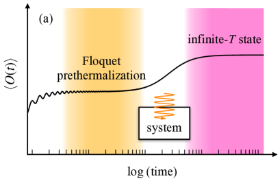
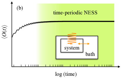
Figure 1: Typical time evolution of an observable $\langle O(t)\rangle$ in (a) periodically driven isolated quantum systems and (b) periodically driven open quantum systems. The former reaches an infinite-temperature steady state through an intermediated quasistationary Floquet prethermal state, while the latter reaches a time-periodic nonequilibrium steady state (NESS).

Periodically driven quantum systems are typically classified into two types: one is the case of isolated quantum systems driven by time-periodic fields, whose time evolution is purely determined by the unitary dynamics. The other is the case of open quantum systems, i.e., systems coupled to environment with dissipation. The dynamics are quite different between them (see Figure 1). The former eventually reaches an infinite-temperature state in the long-time limit (Lazarides et al., 2014; D’Alessio and Rigol, 2014; Ponte et al., 2015a), since the energy is continuously supplied to the system by the periodic driving, which turns into heat in general (nonintegrable) systems. Before approaching the infinite-temperature state, the system may stay at an intermediate quasi-stationary state (called Floquet prethermalization) for a certain time scale, which becomes exponentially long when the driving frequency is relatively high as compared to the system’s energy scale (Mori et al., 2016; Kuwahara et al., 2016; Abanin et al., 2017; Mori et al., 2018). The latter, on the other hand, may arrive at a time-periodic nonequilibrium steady state (NESS), in which the energy absorbed from the external field is balanced with that dissipating into environment (Tsuji et al., 2009; Oka and Aoki, 2009; Dehghani et al., 2014; Mikami et al., 2016; Shirai et al., 2016; Murakami et al., 2017; Ikeda and Sato, 2020).

In addition to these typical cases, nontrivial time-periodic stationary states are known to emerge in driven many-body localized systems, where heating is avoided without coupling to environment due to the effect of strong disorder (Ponte et al., 2015b; Lazarides et al., 2015; Abanin et al., 2016) and the emergence of approximately conserved charges (Das, 2010; Haldar et al., 2018; Haldar and Das, 2022). Recent studies (Sacha, 2015; Khemani et al., 2016; Else et al., 2016; Yao et al., 2017; Moessner and Sondhi, 2017) have unveiled another possibility that time-periodic steady states in periodically driven quantum systems can possess a different periodicity than that of the driving field, which is referred to as a (discrete) time crystal in the sense that the discrete time translation symmetry is spontaneously broken (as in the space translation symmetry broken in a crystal). In this way, the landscape of stationary states in periodically driven quantum systems is widely broadened, and many different types of quasiparticles can be found there.

III Floquet theory

In quantum mechanics, the Floquet theory plays a fundamental role in describing Floquet states that emerge under an application of time-periodic driving fields. In the case of isolated quantum systems, the time evolution is determined by the time-dependent Schrödinger equation,

$$i\frac{d}{dt}|\psi(t)\rangle =H(t)|\psi(t)\rangle,$$ (1)

where $|\psi(t)\rangle$ and $H(t)$ are the system’s wavefunction and hermitian Hamiltonian, respectively, and we set $\hbar=1$ throughout the article. The Hamiltonian is assumed to have time periodicity, $H(t+T)=H(t)$, with a period $T$ (and frequency $\omega=2\pi/T$). The formal solution to the Schrödinger equation (1) is written as $|\psi(t)\rangle=U(t,t_{0})|\psi(t_{0})\rangle$ ($t\geq t_{0}$), where $U(t,t_{0})$ is the unitary evolution operator defined by

$$U(t,t_{0}) :=\mathcal{T}\exp\left(-i\int_{t_{0}}^{t}d\bar{t}\,H(\bar{t})\right)$$ (2)

with $\mathcal{T}$ representing the time-ordered product.

The spirit of the Floquet theory lies in the idea of decomposing the overall dynamics into stroboscopic evolution (i.e., a sequence of snapshots at times $s\to s+T\to s+2T\to\cdots$) and micromotion (i.e., $s\to s+t$ ($0\leq t<T$)). The former contains information about long-time and time-averaged dynamics, while the latter includes information on fast dynamics in a short-time scale. To describe stroboscopic dynamics, it is convenient to consider time evolution by one cycle, starting from time $s$,

$$U(s+T,s) =:e^{-iH_{F}(s)T},$$ (3)

where we define a hermitian operator $H_{F}(s)$ as an effective ‘static’ Hamiltonian that describes time evolution over one period. Alternatively, one can write $H_{F}(s)=iT^{-1}\log U(s+T,s)$. The eigenvalues of $H_{F}(s)$ are determined only up to modulo $\omega=2\pi/T$. Once $H_{F}(s)$ is known, stroboscopic dynamics from $s$ to $s+nT$ ($n=1,2,3,\dots$) is given by $U(s+nT,s)=e^{-inH_{F}(s)T}$. In general, however, $H_{F}(s)$ is a highly non-local and complicated many-body operator.

For general time evolution, one can rewrite the unitary operator $U(t,t_{0})$ (2) as

$$U(t,t_{0}) =U(t,s)e^{i(t-s)H_{F}(s)}e^{-i(t-t_{0})H_{F}(s)}$$

$$\quad\times e^{-i(t_{0}-s)H_{F}(s)}U(s,t_{0})$$ (4)

with a free parameter $s$. The above equation indicates how $U(t,t_{0})$ differs from $e^{-i(t-t_{0})H_{F}(s)}$. If $t_{0}=s$ and $t=s+T$, the two are identical, while in other cases they are not in general. The discrepancy between $U(t,t_{0})$ and $e^{-i(t-t_{0})H_{F}(s)}$ is characterized by a unitary operator

$$P_{s}(t) :=U(t,s)e^{i(t-s)H_{F}(s)},$$ (5)

which is time periodic ($P_{s}(t+T)=P_{s}(t)$) by construction. Using $P_{s}(t)$ (5), one can express the time-evolution operator as

$$U(t,t_{0}) =P_{s}(t)e^{-i(t-t_{0})H_{F}(s)}P_{s}(t_{0})^{-1}.$$ (6)

Now we are in a position to state Floquet’s theorem in the present context.

(Floquet’s theorem) Given a time-periodic Hamiltonian $H(t)=H(t+T)$ and the corresponding unitary evolution operator $U(t,t_{0})$ (2), there exist a time-independent hermitian operator $H_{F}$ and a time-periodic unitary operator $P(t)=P(t+T)$ such that

$$U(t,t_{0}) =P(t)e^{-i(t-t_{0})H_{F}}P(t_{0})^{-1}.$$ (7)

Since we have already given an example of explicit constructions of the operators $H_{F}$ and $P(t)$ in the above (Eqs. (3) and (5)), the proof of the theorem has been completed. The operator $H_{F}$ and its eigenvalues are often referred to as Floquet Hamiltonian and quasienergies, respectively. If one substitutes Eq. (7) in the equation of motion, $i\partial_{t}U(t,t_{0})=H(t)U(t,t_{0})$, one obtains a relation between $H_{F}$ and $P(t)$,

$$H_{F} =P(t)^{-1}\left(H(t)-i\partial_{t}\right)P(t).$$ (8)

The choice of the combination $\{H_{F},P(t)\}$ is not unique. This can be seen in the previous example, where $H_{F}(s)$ (3) and $P_{s}(t)$ (5) depend on the free parameter $s$. On the other hand, $\{H_{F},P(t)\}$ does not necessarily correspond to $\{H_{F}(s),P_{s}(t)\}$ for certain $s$.

Although the combination $\{H_{F},P(t)\}$ is not unique, the eigenvalues of $H_{F}$ are unique (up to mod $\omega$). Suppose that there exist two pairs, $\{H_{F},P(t)\}$ and $\{\tilde{H}_{F},\tilde{P}(t)\}$, that satisfy Eq. (7). By defining a unitary operator $V(t_{0}):=P(t_{0})^{-1}\tilde{P}(t_{0})$, one can see that they are related through

$$e^{-i\tilde{H}_{F}T} =V(t_{0})^{-1}e^{-iH_{F}T}V(t_{0}),$$ (9)

$$\tilde{P}(t) =P(t)e^{-i(t-t_{0})H_{F}}V(t_{0})e^{i(t-t_{0})\tilde{H}_{F}}.$$ (10)

These are a kind of ‘gauge transformations’ that characterize non-uniqueness of $\{H_{F},P(t)\}$. Note that $e^{-i\tilde{H}_{F}T}$ is related to $e^{-iH_{F}T}$ through the unitary transformation, hence the eigenvalues of $H_{F}$ and $\tilde{H}_{F}$ are identical up to mod $\omega$ (except for the difference in order). It is always possible to choose a gauge in such a way that $P(t_{0})=I$ (the identity operator). If $P(t_{0})\neq I$, one can perform a gauge transformation with $V(t_{0})=P(t_{0})^{-1}$, which gives $\tilde{P}(t_{0})=I$. In this particular gauge, the unitary operator is simplified to $U(t,t_{0})=P(t)e^{-i(t-t_{0})H_{F}}$.

The wavefunction evolves, according to Floquet’s theorem (7), as $|\psi(t)\rangle=P(t)e^{-i(t-t_{0})H_{F}}P(t_{0})^{-1}|\psi(t_{0})\rangle$. If $P(t_{0})^{-1}|\psi(t_{0})\rangle$ is an eigenstate (say $|\psi_{\alpha}\rangle$) of $H_{F}$ (with an eigenvalue $\varepsilon_{\alpha}$), the wavefunction takes a form of

$$|\psi(t)\rangle =e^{-i\varepsilon_{\alpha}(t-t_{0})}|u_{\alpha}(t)\rangle$$ (11)

with $|u_{\alpha}(t)\rangle:=P(t)|\psi_{\alpha}\rangle$, which is time periodic, $|u_{\alpha}(t+T)\rangle=|u_{\alpha}(t)\rangle$. Thus, the wavefunction is decomposed into the phase factor and the time-periodic part in Eq. (11). This is analogous to the well-known Bloch’s theorem for spatially periodic systems in solid-state physics, in which the Bloch wavefunction has a form of the product of a plane wave and a spatially periodic function (see Table 1 for comparison).

If $P(t_{0})^{-1}|\psi(t_{0})\rangle$ is not an eigenstate of $H_{F}$, one can still expand it in the complete eigenbasis of the hermitian operator $H_{F}$, $\{|\psi_{\alpha}\rangle\}_{\alpha}$ , as

$$P(t_{0})^{-1}|\psi(t_{0})\rangle =\sum_{\alpha}c_{\alpha}|\psi_{\alpha}\rangle.$$ (12)

Then the wavefunction at time $t$ is given by

$$|\psi(t)\rangle =\sum_{\alpha}c_{\alpha}e^{-i\varepsilon_{\alpha}(t-t_{0})}|u_{\alpha}(t)\rangle,$$ (13)

where $c_{\alpha}$ is a time-independent coefficient. Again, the wavefunction is expressed as a combination of the phase factors and the time-periodic functions $|u_{\alpha}(t)\rangle$.

	Bloch	Floquet
Hamiltonian	$H(\boldsymbol{r}+\boldsymbol{R})=H(\boldsymbol{r})$	$H(t+T)=H(t)$
wavefunction	$|\psi_{\boldsymbol{k}}(\boldsymbol{r})\rangle=e^{i\boldsymbol{k}\cdot\boldsymbol{r}}|u_{\boldsymbol{k}}(\boldsymbol{r})\rangle,$	$|\psi_{\alpha}(t)\rangle=e^{-i\varepsilon_{\alpha}t}|u_{\alpha}(t)\rangle,$
	$|u_{\boldsymbol{k}}(\boldsymbol{r}+\boldsymbol{R})\rangle=|u_{\boldsymbol{k}}(\boldsymbol{r})\rangle$	$|u_{\alpha}(t+T)\rangle=|u_{\alpha}(t)\rangle$
	(crystal momentum $\boldsymbol{k}$)	(quasienergy $\varepsilon_{\alpha}$)
Brillouin zone	$\displaystyle-\frac{\pi}{a}\leq\boldsymbol{k}_{i}<\frac{\pi}{a}$	$\displaystyle-\frac{\omega}{2}\leq\varepsilon<\frac{\omega}{2}$

Table 1: Comparison between Bloch’s theorem for spatially periodic systems and Floquet’s theorem for time-periodic systems. The Brillouin zone in momentum space is shown for a simple cubic lattice with a lattice constant $a$ as an example.

An observable $\langle O(t)\rangle=\langle\psi(t)|O|\psi(t)\rangle$ is not necessarily time periodic due to the presence of off-diagonal terms in the Floquet eigenbasis, $e^{i(\varepsilon_{\alpha}-\varepsilon_{\beta})(t-t_{0})}\langle u_{\alpha}(t)|O|u_{\beta}(t)\rangle$ ($\alpha\neq\beta$). However, there are various situations where the contributions of the off-diagonal terms are suppressed, such as Floquet prethermalized states in an isolated system and nonequilibrium steady states in open systems (Figure 1). In those cases, time evolution of observables becomes periodic with the same periodicity as the driving field. An important exception is a discrete time crystal (Sacha, 2015; Khemani et al., 2016; Else et al., 2016; Yao et al., 2017; Moessner and Sondhi, 2017), where observables become time periodic but its periodicity is integer multiples of that of the driving field.

One can look at Floquet’s theorem from another point of view, which is even closer to that of solid-state physics, i.e., the band picture. By substituting the Floquet wavefunction (11) into the time-dependent Schrödinger equation (1), one obtains $i\frac{d}{dt}|u_{\alpha}(t)\rangle+\varepsilon_{\alpha}|u_{\alpha}(t)\rangle=H(t)|u_{\alpha}(t)\rangle$. Since $|u_{\alpha}(t)\rangle$ and $H(t)$ are both periodic in time, one can Fourier transform them into Fourier modes,

$$H_{mn} :=T^{-1}\int_{0}^{T}dt\,e^{i(m-n)\omega t}H(t),$$ (14)

$$|u_{\alpha}^{n}\rangle :=T^{-1}\int_{0}^{T}dt\,e^{in\omega t}|u_{\alpha}(t)\rangle.$$ (15)

Since $H_{mn}$ only depends on $m-n$, one can also use a shorthand notation of $H_{m-n}:=H_{mn}$. After that, the time-dependent Schrödinger equation turns into a seemingly time-independent equation,

$$\sum_{n}\mathcal{(}\mathcal{H}_{F})_{mn}|u_{\alpha}^{n}\rangle=\varepsilon_{\alpha}|u_{\alpha}^{m}\rangle,$$ (16)

$$(\mathcal{H}_{F})_{mn}:=H_{mn}-m\omega\delta_{mn}.$$ (17)

Here comes an idea of extending the Hilbert space in order to interpret Eq. (16) as an eigenvalue problem. Let $\mathbb{H}$ be the Hilbert space of the system, and let $\mathbb{T}$ be a vector space spanned by Fourier modes of time-periodic functions with the period $T$. For example, a periodic function $f(t)=f(t+T)$ is Fourier transformed as $f(t)=\sum_{n}f_{n}e^{-in\omega t}$. Then a vector $(\cdots,f_{-2},f_{-1},f_{0},f_{1},f_{2},\cdots)$, whose elements are composed of Fourier coefficients, belongs to $\mathbb{T}$. Equation (16) can be viewed as an eigenvalue equation in the extended Hilbert space $\mathbb{H}\otimes\mathbb{T}$ (Sambe space (Sambe, 1973)).

The set $\{\varepsilon_{\alpha}\}_{\alpha}$ has been defined as the eigenvalues of $H_{F}$ acting on $\mathbb{H}$, while in Eq. (16) they appear as the eigenvalues of $\mathcal{H}_{F}$ acting on $\mathbb{H}\otimes\mathbb{T}$. Since the dimensions of $\mathbb{H}$ and $\mathbb{H}\otimes\mathbb{T}$ are different, there must be missing eigenvalues of $\mathcal{H}_{F}$, which can be found if one notices the fact that a vector $|u_{\alpha}^{n-l}\rangle$ shifted from $|u_{\alpha}^{n}\rangle$ by $l$ components ($l=0,\pm 1,\pm 2,\dots$) is also an eigenstate of $\mathcal{H}_{F}$ with an eigenvalue $\varepsilon_{\alpha}-l\omega$. This means that $\{|u_{\alpha}^{n-l}\rangle\}_{\alpha,l}$ consists of a complete set of the eigenstates in $\mathbb{H}\otimes\mathbb{T}$. The spectrum of the corresponding eigenvalues $\{\varepsilon_{\alpha}-l\omega\}_{\alpha,l}$ shows a periodic structure in energy space, in much the same way as the band structure shows a periodic pattern in momentum space for spatially periodic systems. In particular, one can restrict the energy space within $-\frac{\omega}{2}\leq\varepsilon_{\alpha}<\frac{\omega}{2}$ (the Floquet Brillouin zone) by shifting quasienergies by integer multiples of $\omega$ in order to represent quasienergies without mod $\omega$ redundancies.

Thus, $H_{F}$ and $\mathcal{H}_{F}$ share the same eigenvalues up to mod $\omega$. As we have mentioned, $H_{F}$ is a complicated non-local many-body operator that is expected to be difficult to evaluate directly, while $\mathcal{H}_{F}$ is usually a well-behaved local few-body operator. On the other hand, the latter is acting on the extended space $\mathbb{H}\otimes\mathbb{T}$, whose dimension is infinitely larger than $\mathbb{H}$. In practice, one can truncate the Fourier space $\mathbb{T}$ to finite dimensions as an approximation; Off-diagonal elements, $(\mathcal{H}_{F})_{mn}$, physically correspond to $m-n$ photon absorption/emission processes, which would be suppressed when $|m-n|\gg 1$ if the drive strength is not too strong.

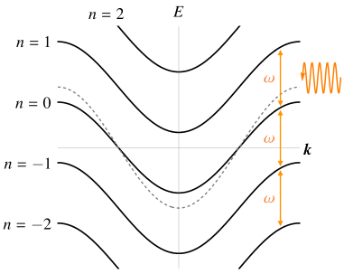
Figure 2: The quasienergy spectrum of noninteracting electrons on a one-dimensional lattice driven by an ac electric field (solid curves). The dashed curve shows the original energy dispersion without the driving field.

IV Examples

As an example, let us consider a single-band system of noninteracting electrons driven by a time-periodic field described by the Hamiltonian

$$H(t) =\sum_{\boldsymbol{k}}\varepsilon_{\boldsymbol{k}}(t)c_{\boldsymbol{k}}^{\dagger}c_{\boldsymbol{k}},$$ (18)

where $c_{\boldsymbol{k}}^{\dagger}$ is a creation operator of electrons with momentum $\boldsymbol{k}$, and $\varepsilon_{\boldsymbol{k}}(t)=\varepsilon_{\boldsymbol{k}}(t+T)$ is a band dispersion including the coupling to a time-periodic field. The eigenvalues (quasienergies) of the corresponding $\mathcal{H}_{F}$ (17) are given by $T^{-1}\int_{0}^{T}dt\,\varepsilon_{\boldsymbol{k}}(t)+n\omega$ ($n=0,\pm 1,\pm 2,\dots$) (Tsuji et al., 2008), i.e., the time-averaged dispersion shifted by integer multiples of the drive frequency $\omega$. One can confirm that these are also eigenvalues of $H_{F}$ (7), since the time evolution operator is given by $U(t,t_{0})=e^{-i\int_{t_{0}}^{t}ds\,\sum_{\boldsymbol{k}}\varepsilon_{\boldsymbol{k}}(s)c_{\boldsymbol{k}}^{\dagger}c_{\boldsymbol{k}}}$ which is free from the time-ordering operator due to $[H(t),H(t^{\prime})]=0$.

If the system is a one-dimensional lattice with a nearest-neighbor hopping with a dispersion $\varepsilon_{k}=-2J\cos k$ driven by an ac electric field with amplitude $E$ (represented by a vector potential $A(t)=-E\sin\omega t/\omega$), the time average of the dispersion is given by $T^{-1}\int_{0}^{T}dt\,(-2J)\cos(k-A(t))=-2J\mathcal{J}_{0}(E/\omega)\cos k$, where the hopping amplitude $J$ is multiplied by $\mathcal{J}_{0}(E/\omega)$, the zeroth-order Bessel-function factor. In Figure 2, we show the corresponding quasienergy spectrum. Due to the presence of the periodic drive, the hopping amplitude is effectively reduced ($|\mathcal{J}_{0}(E/\omega)|\leq 1$), and electrons become heavier. When the Bessel factor exactly vanishes ($\mathcal{J}_{0}(E/\omega)=0$), electrons cannot hop to neighboring sites completely, resulting in dynamical localization (Dunlap and Kenkre, 1986; Holthaus, 1992). In the spectrum (Fig. 2), there are side-band structures (labeled by the Fourier mode index $n$) separated by $\omega$ from the neighboring bands, which is referred to as the dynamic Wannier-Stark ladder. These arise due to the consequence of virtual $n$-photon absorption/emission processes.

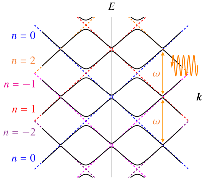
Figure 3: The quasienergy spectrum (solid curves) of Dirac electrons driven by circularly polarized light ($A=1,\omega=5$). The dashed lines with Fourier mode labels $n$ show the spectrum without driving.

Another example is a model of Dirac electrons in two spatial dimensions driven by circularly polarized light (Oka and Aoki, 2009; Mikami et al., 2016). The Hamiltonian reads

$$H(t) =\sum_{\boldsymbol{k}\alpha\beta}c_{\boldsymbol{k}\alpha}^{\dagger}h_{\boldsymbol{k}\alpha\beta}(t)c_{\boldsymbol{k}\beta},$$ (19)

$$h_{\boldsymbol{k}\alpha\beta}(t) =(k_{x}-A_{x}(t))(\sigma_{x})_{\alpha\beta}+(k_{y}-A_{y}(t))(\sigma_{y})_{\alpha\beta},$$ (20)

where $c_{\boldsymbol{k}\alpha}^{\dagger}$ is a creation operator of electrons with two components (corresponding to two bands near the Fermi energy), $(A_{x},A_{y})=(A\cos\omega t,A\sin\omega t)$ is the vector potential for circularly polarized light, and $\sigma_{x}$ and $\sigma_{y}$ are Pauli matrices. In this system, circularly polarized light explicitly breaks time reversal symmetry.

In Figure 3, a typical quasienergy spectrum is shown. When the driving field is absent, the spectrum consists of a Dirac cone (linear dispersion) without energy gap near $E=0$. As one increases the amplitude of the electric field, there emerge energy gaps at the band crossing points, accompanied by sideband structures with energy spacing $\omega$. Especially, at $\boldsymbol{k}=0$ the gap is given by $\Delta=\sqrt{\omega^{2}+4A^{2}}-\omega$ (Oka and Aoki, 2009). This phenomenon, light-induced gap opening in the quasienergy spectrum (accompanied by chiral edge modes), can be interpreted as a topological phase transition, since quasienergy bands are characterized by non-zero topological (Chern) numbers, similar to quantum Hall states in static systems. In this sense, the system is classified to a Floquet topological insulator (Oka and Aoki, 2009; Kitagawa et al., 2010, 2011; Lindner et al., 2011; Roy and Harper, 2017; Rudner and Lindner, 2020), a class of topological phases in periodically driven systems.

While the above example can be understood by mapping to the corresponding static model, there are several examples that show nontrivial topological phases that do not have equilibrium counterparts (Kitagawa et al., 2010, 2012; Rudner et al., 2013; Harper et al., 2020; Nakagawa et al., 2020a; Jangjan et al., 2022): Topologically protected chiral edge modes can appear even though all the bulk Floquet bands have vanishing Chern numbers. This is possible since in Floquet systems edge modes can go across the quasienergy $\varepsilon=\pm\pi/T$ (‘anomalous $\pi$ modes’) and wind around the Floquet Brillouin zone in the frequency domain. In this case, the system is called an anomalous Floquet topological insulator.

V High-frequency expansion

The approach of the Floquet theory becomes particularly effective when the drive frequency is higher than typical energy scales included in the original (un-driven) Hamiltonian. Intuitively, when the frequency is sufficiently large, physical degrees of freedom in the system cannot follow rapid oscillations of the drive field. As a result, the effect of the drive is rounded in the time average, implying that the Floquet Hamiltonian $H_{F}$ defined in Floquet’s theorem (7) is approximated to be the time average of the original Hamiltonian, $H_{F}\approx H_{0}=T^{-1}\int_{0}^{T}dt\,H(t)$. This intuition is actually justified in the form of high-frequency expansions (or $1/\omega$ expansion), a typical one of which reads

$$H_{F} =H_{0}+\sum_{n=1}^{\infty}\frac{[H_{-n},H_{n}]}{n\omega}+\cdots,$$ (21)

where “$\cdots$” contains higher-order terms in $1/\omega$. The second term on the right-hand side of Eq. (21) can be understood as a sum of second-order perturbation corrections for $n$-photon absorption/emission processes.

There are several ways to carry out such an expansion (e.g., Floquet-Magnus expansion (Fel’dman, 1984; Casas et al., 2001; Blanes et al., 2009; Mananga and Charpentier, 2011; Goldman and Dalibard, 2014), van Vleck perturbation theory (Eckardt and Anisimovas, 2015; Bukov et al., 2015), Brillouin-Wigner perturbation theory (Mikami et al., 2016), etc.), all of which are known to be equivalent to each other in the sense that they all give the same high-frequency expansion for the eigenvalues of $H_{F}$ (up to mod $\omega$). One can derive some of them, for example, by starting from Eq. (8), $H_{F}=e^{i\Lambda(t)}(H(t)-i\partial_{t})e^{-i\Lambda(t)}$, where $\Lambda(t)$ is a hermitian operator defined by $P(t)=:e^{-i\Lambda(t)}$. This relation can be rewritten with an adjoint operator ${\rm ad}_{\Lambda(t)}X:=[\Lambda(t),X]$ as

$$\frac{d}{dt}\Lambda(t) =\sum_{n=0}^{\infty}\frac{B_{n}}{n!}(-i)^{n}({\rm ad}_{\Lambda(t)})^{n}[H(t)+(-1)^{n+1}H_{F}],$$ (22)

where $B_{n}$ is the Bernoulli number. One can solve Eq. (22) order-by-order by expanding

$$\Lambda(t) =\sum_{k=1}^{\infty}\Lambda^{(k)}(t),\quad H_{F}=\sum_{k=0}^{\infty}H_{F}^{(k)},$$ (23)

where one assigns an order 1 for $H(t)$, the order $k$ for $\Lambda^{(k)}$, and the order $k+1$ for $H^{(k)}$. In this rule, the superscript $(k)$ of $\Lambda^{(k)}$ and $H^{(k)}$ represents the order in $1/\omega$.

To determine the expansion, one needs to fix the gauge. For example, one can set $\Lambda(t_{0})=0$ at certain time $t_{0}$, which generates the so-called Floquet-Magnus expansion. While the expansion can be uniquely determined, there remains a spurious dependence on $t_{0}$ that appears as a phase factor in the expansion. Another choice that is often employed is $\int_{0}^{T}dt\,\Lambda(t)=0$, which corresponds to the van Vleck perturbation expansion (Eq. 21) that does not have explicit $t_{0}$ dependence. These two expansions are related through unitary transformation.

The high-frequency expansions are usually asymptotic expansions. That is, they do not converge in the ordinary sense but give good approximation if the infinite series are truncated at a certain finite order. In fact, there is a rigorous estimate for the error induced by such a truncation, which suggests that the truncated Floquet-Magnus expansion accurately describes time evolution of periodically driven quantum systems up to a time scale which is exponentially long as a function of drive frequency. As a result, there emerges an exponentially long-lived prethermal regime (Fig. 1(a)) at an early stage of periodic driving, where the system shows thermal behavior with respect to the effective Hamiltonian given by the truncated expansion.

As an example, let us apply the high-frequency expansion to a model of noninteracting electrons on a honeycomb lattice driven by circularly polarized light. The Hamiltonian is given by

$$H(t) =J\sum_{\langle jk\rangle}\left[\exp\left(-i\int_{\boldsymbol{R}_{k}}^{\boldsymbol{R}_{j}}\boldsymbol{A}(t)\cdot d\boldsymbol{r}\right)c_{j}^{\dagger}c_{k}+\mbox{h.c.}\right],$$ (24)

where $\langle jk\rangle$ denotes nearest-neighbor sites at positions $\boldsymbol{R}_{j}$ and $\boldsymbol{R}_{k}$ on the honeycomb lattice, and $\boldsymbol{A}(t)$ represents a vector potential for circularly polarized light, which is included as a Peierls phase. In the high-frequency expansion (21), the corresponding effective Hamiltonian is given by (Mikami et al., 2016)

$$H_{F} =J_{\rm eff}\sum_{\langle jk\rangle}(c_{j}^{\dagger}c_{k}+\mbox{h.c.})+K_{\rm eff}\sum_{\langle\!\langle jk\rangle\!\rangle}(i\tau_{j,k}c_{j}^{\dagger}c_{k}+\mbox{h.c.})$$

$$\quad+O\left(\frac{1}{\omega^{2}}\right),$$ (25)

where $\langle\!\langle jk\rangle\!\rangle$ represents next-nearest-neighbor sites, $J_{\rm eff}=J\mathcal{J}_{0}(A)$, $K_{\rm eff}=-J^{2}/\omega\sum_{n\neq 0}\mathcal{J}_{n}(A)^{2}\sin(2\pi n/3)/n$ ($\mathcal{J}_{n}(A)$ is the $n$th-order Bessel function), and $\tau_{j,k}=\pm 1$ represents the chirality of the hopping from $k$ to $j$ ($+$($-$) is assigned to the clockwise (counterclockwise) path on a hexagon).

In addition to the modulated nearest-neighbor hopping, there appear next-nearest-neighbor hoppings that are purely imaginary. The resulting Hamiltonian is equivalent to the Haldane model (Haldane, 1988), a tight-binding model on a honeycomb lattice with complex next-nearest-neighbor hoppings, which is known to be a model of quantum anomalous Hall states (Chern insulators). Thus, one can understand that the system undergoes a topological phase transition induced by circularly polarized light. This is consistent with the result of the model of Dirac electrons treated in the previous section. As one reduces the drive frequency, higher-order terms in the high-frequency expansion become relevant, and more complicated topological phases can be found with high Chern numbers (Mikami et al., 2016).

VI Periodically driven open quantum systems

In open quantum systems, the time evolution of the system is not simply given by the time-dependent Schrödinger equation (1) due to the effect of environment. Let the total Hamiltonian be given as $H=H_{S}+H_{I}+H_{B}$, where $H_{S}$ is the system’s Hamiltonian, $H_{I}$ represents the interaction between the system and environment, and $H_{B}$ is the Hamiltonian of environment (bath). The density matrix of the total system $\rho$ evolves according to the von Neumann equation, $\frac{d}{dt}\rho=-i[H,\rho]$. What one is interested in here is the time evolution of the system’s density matrix defined by $\rho_{S}={\rm tr}_{B}\rho$ (${\rm tr}_{B}$ denotes the partial trace over environment’s degrees of freedom).

One approach to describe the system’s dynamics is to use a quantum Master equation, which is a quantum analog of Master equations in classical stochastic processes (Breuer and Petruccione, 2007). To derive the quantum Master equation, there are two basic assumptions: (i) Markovianity of system’s time evolution (i.e., $\rho_{S}(t+\Delta t)$ is solely determined from $\rho_{S}(t)$), and (ii) absence of initial correlations between the system and environment (i.e., $\rho(0)=\rho_{S}(0)\otimes\rho_{B}(0)$). In this situation, if a map from arbitrary $\rho_{S}(0)$ to $\rho_{S}(t)$ is completely positive and trace preserving, $\rho_{S}(t)$ obeys the following form of the quantum Master equation (Gorini-Kossakowski-Sudarshan-Lindblad equation (Gorini et al., 1976; Lindblad, 1976)),

$$\frac{d}{dt}\rho_{S} =-i[H_{S},\rho_{S}]+\sum_{j}\left(L_{j}\rho_{S}L_{j}^{\dagger}-\frac{1}{2}\{L_{j}^{\dagger}L_{j},\rho_{S}\}\right),$$ (26)

with a certain set of operators $\{L_{j}\}$ called Lindblad operators (or jump operators). The second term on the right-hand side of Eq. (26) represents the effect of environment, giving non-unitary dynamics. If one defined a non-hermitian effective Hamiltonian, $H_{\rm eff}:=H_{S}-\frac{i}{2}\sum_{j}L_{j}^{\dagger}L_{j}$, Eq. (26) is rewritten as

$$\frac{d}{dt}\rho_{S} =-i(H_{\rm eff}\rho_{S}-\rho_{S}H_{\rm eff}^{\dagger})+\sum_{j}L_{j}\rho_{S}L_{j}^{\dagger}.$$ (27)

The second term on the right-hand side of Eq. (27) represents quantum jump processes, in which the system’s state discontinuously changes in a stochastic manner.

A microscopic justification of the quantum Master equation (26) often requires additional approximations. The conventional approach employs (i) the Born approximation which is valid for the weak coupling between the system and environment and (ii) the secular approximation (or the rotating-wave approximation) that can be justified when the inverse of the level spacing between the eigenvalues of $H_{S}$ is much smaller than the relaxation time of the system. The latter condition does not usually hold for many-body systems, since the level spacing becomes exponentially small as the system size increases. Nevertheless, the quantum Master equation has been used from a phenomenological point of view to describe the dynamics of open quantum many-body systems (Diehl et al., 2010; Prosen, 2011; Tindall et al., 2019; Nakagawa et al., 2020b; Yamamoto et al., 2021).

In the presence of periodic driving, the use of the quantum Master equation needs more careful derivation (Mori, 2023). Especially, if one is interested in nontrivial nonequilibrium steady states, heating due to the periodic drive should be balanced with dissipation. The relaxation time then becomes comparable to the system’s intrinsic time scale, which may invalidate the secular approximation. There has recently been a proposal for the derivation of quantum Master equations without relying on the secular approximation (or the rotating-wave approximation) (Nathan and Rudner, 2020, 2022). The underlying notion is that Markovianity is a property of the bath and the system-bath coupling solely, and should not depend on details of the energy level structure of the system. In fact, one can derive a Markovian quantum Master equation (called the ‘universal Lindblad equation’) when the correlation time of the bath is much shorter than the characteristic time scale of the system-bath interaction.

Another approach to driven open quantum systems is to use nonequilibrium Green’s functions (Kadanoff and Baym, 1962; Keldysh, 1965). The advantage of this approach is that it does not necessarily rely on the Markov and secular approximations. On the other hand, since the approach is based on the Green’s function formalism, one has to adopt certain diagrammatic techniques to treat many-body interactions.

One of the simplest models of environment for electrons is a free-fermion heat bath (Tsuji et al., 2009; Aoki et al., 2014), whose Hamiltonians are given by

$$H_{B} =\sum_{j,k}\varepsilon_{k}b_{j,k}^{\dagger}b_{j,k},$$ (28)

$$H_{I} =\sum_{j,k}V_{k}(c_{j}^{\dagger}b_{j,k}+{\rm h.c.}),$$ (29)

where $c_{j}^{\dagger}$ and $b_{j,k}^{\dagger}$ are creation operators of system’s and bath’s electrons at site $j$ and mode $k$, respectively, $\varepsilon_{k}$ is the energy of bath’s electrons, and $V_{k}$ is a coupling between system’s and bath’s electrons. The system’s retarded, advanced, and Keldysh Green’s functions are defined as

$$G_{ij}^{R}(t,t^{\prime}) =-i\theta(t-t^{\prime})\langle\{c_{i}(t),c_{j}^{\dagger}(t^{\prime})\}\rangle,$$ (30)

$$G_{ij}^{A}(t,t^{\prime}) =i\theta(t^{\prime}-t)\langle\{c_{i}(t),c_{j}^{\dagger}(t^{\prime})\}\rangle,$$ (31)

$$G_{ij}^{K}(t,t^{\prime}) =-i\langle[c_{i}(t),c_{j}^{\dagger}(t^{\prime})]\rangle,$$ (32)

respectively ($\theta(t)$ is the step function). The retarded (and advanced) Green’s function contains information about the single-particle spectrum of the system, while the Keldysh one carries information about the occupation distribution of the spectrum.

Since the total Hamiltonian $H=H_{S}+H_{I}+H_{B}$ is quadratic in $b_{j,k}^{\dagger}$ and $b_{j,k}$, one can integrate out the bath’s degrees of freedom analytically. As a result, the system’s Green’s function satisfies the following Dyson equation,

$$\begin{pmatrix}G^{R}&G^{K}\\ 0&G^{A}\end{pmatrix} =\Bigg{[}\begin{pmatrix}G_{0}^{R}&G_{0}^{K}\\ 0&G_{0}^{A}\end{pmatrix}^{-1}-\begin{pmatrix}\Sigma_{b}^{R}&\Sigma_{b}^{K}\\ 0&\Sigma_{b}^{A}\end{pmatrix}$$

$$\quad-\begin{pmatrix}\Sigma^{R}&\Sigma^{K}\\ 0&\Sigma^{A}\end{pmatrix}\Bigg{]}^{-1},$$ (33)

where $G_{0}$ is the system’s noninteracting Green’s function, $\Sigma_{b}$ is the self-energy due to the coupling to the heat bath, and $\Sigma$ is the system’s self-energy. For the free-fermion bath, the retarded component of $\Sigma_{b}$ is explicitly given in the frequency domain as

$$\Sigma_{b}^{R}(\nu) =\sum_{k}\frac{V_{k}^{2}}{\nu-\varepsilon_{k}+i\eta},$$ (34)

where $\eta$ is an infinitesimal positive constant. By using $1/(\nu+i\eta)=\mathcal{P}(1/\nu)-i\pi\delta(\nu)$ (with $\mathcal{P}$ being the principal value), one obtains the imaginary part of $\Sigma_{b}^{R}(\nu)$,

$$\Gamma(\nu) =\sum_{k}\pi V_{k}^{2}\delta(\nu-\varepsilon_{k}),$$ (35)

which corresponds to the bath’s spectral function. One often assumes a flat density of states for the bath, $\Gamma(\nu)=\Gamma$, as the simplest choice. The real part of $\Sigma_{b}^{R}(\nu)$ gives a potential shift, which can be renormalized into the chemical potential. The advanced component is simply the complex conjugate, $\Sigma_{b}^{A}(\nu)=\Sigma_{b}^{R}(\nu)^{\dagger}$. The Keldysh part of $\Sigma_{b}$ is determined from the fluctuation-dissipation relation for the bath’s Green’s function, giving $\Sigma_{b}^{K}(\nu)=F(\nu)[\Sigma_{b}^{R}(\nu)-\Sigma_{b}^{A}(\nu)]$ with $F(\nu)=\tanh(\beta\nu/2)$ ($\beta$ is the inverse temperature of the heat bath).

To summarize, the self-energy due to the coupling to the free-fermion bath takes a simple form,

$$\begin{pmatrix}\Sigma_{b}^{R}(\nu)&\Sigma_{b}^{K}(\nu)\\ 0&\Sigma_{b}^{A}(\nu)\end{pmatrix} =\begin{pmatrix}-i\Gamma&-2i\Gamma F(\nu)\\ 0&i\Gamma\end{pmatrix}.$$ (36)

Although the free-fermion bath model looks somewhat artificial, it correctly reproduces the semiclassical result of Boltzmann’s transport theory (Han, 2013; Aoki et al., 2014). In this context, the model can be viewed as a two-parameter phenomenology (the relaxation rate $\Gamma$ and heat bath’s temperature $\beta^{-1}$) to describe dissipation. One can also employ other models for a heat bath such as a model of phonons, but then the bath’s degrees of freedom cannot be integrated out analytically, and one has to use certain approximations.

One can incorporate the effect of periodic driving in this approach. To this end, one assumes the existence of time-periodic nonequilibrium steady states. Once the steady state is reached, the Green’s function should satisfy the periodicity in two-time arguments, $G^{\alpha}(t,t^{\prime})=G^{\alpha}(t+T,t^{\prime}+T)$ ($\alpha=R,A,K$). This allows one to define the Floquet Green’s function (Faisal, 1989; Martinez, 2003, 2005; Tsuji et al., 2008; Aoki et al., 2014; Liu et al., 2017),

$$G_{mn}^{\alpha}(\nu)$$

$$:=\frac{1}{T}\int_{0}^{T}ds\int_{-\infty}^{\infty}dt\,e^{i(m-n)\omega s+i\nu t}G^{\alpha}\left(s+\frac{t}{2},s-\frac{t}{2}\right),$$ (37)

which takes a matrix form with indices $m$ and $n$ being the labels of Fourier modes as used in Eq. (14). The Dyson equation maintains the form of Eq. (33) with all the Green’s functions and self-energies written in the above matrix form with the inverse interpreted as the matrix inverse. The Floquet matrix form of $\Sigma_{b}$ reads $\Sigma_{b,mn}^{R}(\nu)=-i\Gamma\delta_{mn}$ and $\Sigma_{b,mn}^{K}(\nu)=-2i\Gamma F(\beta(\nu+n\omega)/2)\delta_{mn}$.

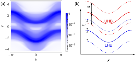
Figure 4: (a) The single-particle spectrum $A(\nu,k)$ of the ac-field-driven Falicov-Kimball model calculated from the Floquet DMFT. (b) The corresponding schematic band structure of the ac-field-driven Mott insulator with the drive frequency $\omega$. The upper and lower Hubbard bands (UHB and LHB) are shown by solid curves, and the accompanied Floquet sidebands are shown by dashed curves. (Adapted from Aoki et al. (2014) Nonequilibrium dynamical mean-field theory and its applications. Rev. Mod. Phys. 86: 779 (Aoki et al., 2014).)

Provided that the self-energy from the system’s interaction is given, the Green’s function in the time-periodic nonequilibrium steady state is determined from the Dyson equation (33). This part requires a (diagrammatic) solver for quantum many-body problems. One such approach is the so-called Floquet dynamical mean-field theory (DMFT) (Tsuji et al., 2008, 2009; Joura et al., 2008; Lubatsch and Kroha, 2009; Aoki et al., 2014), which is a combined formulation of the Floquet theory and nonequilibrium DMFT (Freericks et al., 2006; Aoki et al., 2014). The latter solves nonequilibrium quantum many-body problems under the local approximation of the self-energy (Georges et al., 1996).

In Fig. 4, an example of the result of the Floquet DMFT is shown for the ac-field-driven Falicov-Kimball model (Tsuji et al., 2008, 2009; Aoki et al., 2014), which is a simple model of correlated electrons that shows a Mott insulator-to-metal transition in equilibrium (Freericks and Zlatić, 2003). There emerges an ac-field-induced midgap state between the upper and lower Hubbard bands as Floquet sidebands with an energy spacing $\omega$. Due to this, the system turns from a Mott-insulating state to an ac-field-induced metallic state. This exemplifies a quantum many-body Floquet state.

The nonequilibrium Green’s function approach not only describes the single-particle properties, but also characterizes two-particle ones such as response functions and transport coefficients. To obtain those quantities, one has to evaluate two-particle Green’s functions on top of the single-particle Green’s function. For example, the transport property of the ac-field-driven Falicov-Kimball model can be identified from the optical conductivity spectrum, which shows a Drude-like peak structure at low energy instead of a Mott gap, indicating that the system indeed becomes metallic due to the effect of the ac field (Tsuji et al., 2009).

VII Experimental observations

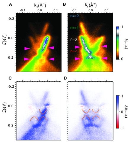
Figure 5: Time-resolved ARPES spectra of surface states of a topological insulator Bi₂Se₃ under circularly polarized laser excitation along (A) $k_{x}$ and (B) $k_{y}$ directions. (C) and (D) are the corresponding spectra after subtracting the spectra at $t=-500$ fs. (Adapted from Wang et al. (2013) Observation of Floquet-Bloch States on the Surface of a Topological Insulator. Science 342: 453-457 (Wang et al., 2013).)

Floquet states have been experimentally observed in various systems. In solid-state materials, occupied single-particle spectra can be measured by angle-resolved photoemission spectroscopy (ARPES), which can map out the band structure of correlated electrons in energy and momentum spaces below the Fermi level. The technique can also be applied to study nonequilibrium states of electrons in solids, in which case pump and probe pulses are applied with a certain time delay in between (time-resolved ARPES). The former pulse is used to drive electrons out of equilibrium, while the latter is used to generate photoelectrons. During irradiation of a pump pulse, the system can be approximately considered to be driven periodically in time if the pump pulse contains sufficiently large number of oscillation cycles. Thus, the time-resolved ARPES offers an opportunity to observe Floquet states for electron systems.

In Fig. 5, an example of time-resolved ARPES spectra is shown for a topological insulator Bi₂Se₃ driven by a circularly polarized laser (Wang et al., 2013). In topological insulators, there are topologically protected gapless surface states, which support an energy dispersion of Dirac cones. This is precisely the same situation as we see in Sec. IV: Dirac electrons driven by circularly polarized light undergoes a transition to a Floquet topological insulator with a gap opening at the Dirac point. In the time-resolved ARPES experiment, the energy gap is observed to appear under the excitation of a circularly polarized laser. On top of that, Floquet sideband structures are observed with the energy spacing of the drive frequency in the ARPES spectra. These are consistent with the results of the Floquet theory (Oka and Aoki, 2009) (see, e.g., Fig. 3). The subsequent experiment has also demonstrated the transition from the Floquet states to Volkov states, i.e., photon-dressed states of free electrons, by time-resolved ARPES (Mahmood et al., 2016).

When Dirac electrons are driven by circularly polarized light and turn to a Floquet topological insulator, the bands around the Dirac point can acquire non-zero Chern numbers. As a result, the system shows the anomalous Hall effect, that is, current flows perpendicular to the direction of an applied dc electric field without a magnetic field. If the distribution of the occupied states are not far from that of zero-temperature equilibrium states, the Hall conductance approaches the quantized value. The Hall conductance of Dirac electrons in a monolayer graphene induced by a circularly polarized laser has been measured experimentally, using an on-chip photoconductive switch device (McIver et al., 2020). The result shows that Floquet topological bands indeed generate the anomalous Hall effect, demonstrating characteristic features of Floquet topological states.

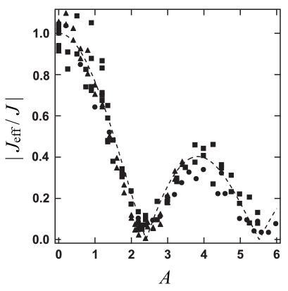
Figure 6: Effective hopping amplitude of Bose-Einstein condensed cold atoms in a periodically shaken optical lattice as a function of the amplitude of the periodic drive. The dashed curve represents the Bessel function $\mathcal{J}_{0}(A)$. (Adapted from Lignier et al. (2007) Dynamical Control of Matter-Wave Tunneling in Periodic Potentials. Phys. Rev. Lett. 99: 220403 (Lignier et al., 2007).)

In contrast to solid-state systems, artificial quantum systems provide high controllability and ideal clean situations to realize Floquet states. For example, cold atomic gases trapped in an optical lattice are well described by a lattice model of isolated quantum many-body systems. One can then drive the system by periodically shaking the optical lattice potential in real space (Eckardt, 2017), mimicking the effect of ac electric fields for electrons.

In Fig. 6, the experimentally measured effective hopping amplitude of Bose-Einstein condensates in a periodically shaken optical lattice is shown as a function of the amplitude $A$ of the periodic drive (Lignier et al., 2007). As we see in Sec. IV and V, the Floquet theory predicts that the hopping amplitude is renormalized by the Bessel factor as $J_{\rm eff}=J\mathcal{J}_{0}(A)$, which perfectly agrees with the experimental observation. Using this effect, one can effectively control the interaction strength with ac fields, inducing, for instance, a superfluid-to-Mott insulator transition in the Bose-Hubbard model (Eckardt et al., 2005). One can even reverse the sign of the hopping if $\mathcal{J}_{0}(A)<0$, which can be used to realize frustrated classical spin systems (Struck et al., 2011) or to effectively convert the interaction from repulsive to attractive in the ac-field-driven Fermi-Hubbard model (Tsuji et al., 2011).

Periodic shaking of optical lattices has also been used to realize the Haldane model in fermionic cold-atom systems (Jotzu et al., 2014), where periodic circular shaking induces the Floquet topological insulator with complex hopping parameters on a honeycomb lattice as discussed above. The generated band gap is probed by momentum-resolved measurement of interband transitions. The effect of Berry curvature has been demonstrated by applying a constant force to atoms and finding an orthogonal drift, in the similar manner as the anomalous Hall effect. The induced Berry curvature has been reconstructed in the entire Brillouin zone experimentally (Fläschner et al., 2016).

Other physical systems that allow experimental observations of Floquet states include photonic systems (Kitagawa et al., 2012; Rechtsman et al., 2013; Maczewsky et al., 2017; Mukherjee et al., 2017; Ozawa et al., 2019), trapped ions (Kiefer et al., 2019), and superconducting qubits (Deng et al., 2015; Roushan et al., 2017).

VIII Summary and outlook

Here we have reviewed basic aspects of Floquet states and their applications to various periodically driven quantum systems. It allows one to control phases of matter dynamically (‘Floquet engineering’ (Bukov et al., 2015; Oka and Kitamura, 2019; Weitenberg and Simonet, 2021)) that may not be realized in equilibrium. While our understanding of Floquet states has been deepened, the inherent potential of Floquet states has not been fully elaborated experimentally, especially in solid-state systems. This may be partly because (i) the required amplitude of electric fields is often large, (ii) one needs ultrafast time resolution to capture driven states during irradiation of a pump pulse, (iii) transitions to higher bands and modulation of the distribution may occur in real materials, (iv) heating will suppress quantum fluctuations, and (v) energy dissipation takes place in complicated ways.

While these will make it a great challenge to realize Floquet states in solids, they can also offer opportunities: The development of new materials and new devices will pave a way to explore the frontier of Floquet states. For example, a recent experiment has shown an ideal behavior of driven two-level systems with the scaling of the Bessel factor up to extremely high orders in a diamond nitrogen-vacancy center (Nishimura et al., 2022). If the interaction between the two-level systems can be implemented in those systems, it will provide an interesting playground of Floquet many-body states. Another opportunity is the effect of dissipation in open quantum systems, which can work in a favorable direction to realize (rather than suppress) new orders and new states of matter in quantum systems. For example, a two-body loss due to inelastic collisions in the Fermi-Hubbard model can effectively change the antiferromagnetic interaction to the ferromagnetic one (Nakagawa et al., 2020b), which has been recently observed in cold-atom systems (Honda et al., 2023). Finally, there has been an experimental progress in probing highly oscillating electronic states through high harmonic generation in solids (Ghimire et al., 2011; Schubert et al., 2014; Luu et al., 2015; Vampa et al., 2015; Hohenleutner et al., 2015), which will be a useful key tool to study Floquet states in the future.

References

- Floquet (1883) G. Floquet, “Sur les équations différentielles linéaires à coefficients périodiques,” Ann. de l’Ecole Norm. Sup. 12, 47 (1883).
- Hill (1886) G. W. Hill, “On the part of the motion of the lunar perigee which is a function of the mean motions of the sun and moon,” Acta Math. 8, 1 (1886).
- Magnus and Winkler (1966) W. Magnus and S. Winkler, Hill’s Equation (John Wiley and Sons, New York, 1966).
- Shirley (1965) J. H. Shirley, “Solution of the Schrödinger Equation with a Hamiltonian Periodic in Time,” Phys. Rev. 138, B979 (1965).
- Sambe (1973) H. Sambe, “Steady States and Quasienergies of a Quantum-Mechanical System in an Oscillating Field,” Phys. Rev. A 7, 2203 (1973).
- Grifoni and Hänggi (1998) M. Grifoni and P. Hänggi, “Driven quantum tunneling,” Phys. Rep. 304, 229 (1998).
- Lazarides et al. (2014) A. Lazarides, A. Das, and R. Moessner, “Equilibrium states of generic quantum systems subject to periodic driving,” Phys. Rev. E 90, 012110 (2014).
- D’Alessio and Rigol (2014) L. D’Alessio and M. Rigol, “Long-time Behavior of Isolated Periodically Driven Interacting Lattice Systems,” Phys. Rev. X 4, 041048 (2014).
- Ponte et al. (2015a) P. Ponte, A. Chandran, Z. Papić, and D. A. Abanin, “Periodically driven ergodic and many-body localized quantum systems,” Ann. Phys. 353, 196 (2015a).
- Mori et al. (2016) T. Mori, T. Kuwahara, and K. Saito, “Rigorous Bound on Energy Absorption and Generic Relaxation in Periodically Driven Quantum Systems,” Phys. Rev. Lett. 116, 120401 (2016).
- Kuwahara et al. (2016) T. Kuwahara, T. Mori, and K. Saito, “Floquet-Magnus theory and generic transient dynamics in periodically driven many-body quantum systems,” Ann. Phys. 367, 96 (2016).
- Abanin et al. (2017) D. Abanin, W. De Roeck, W. W. Ho, and F. Huveneers, “A Rigorous Theory of Many-Body Prethermalization for Periodically Driven and Closed Quantum Systems,” Commun. Math. Phys. 354, 809–827 (2017).
- Mori et al. (2018) T. Mori, T. N. Ikeda, E. Kaminishi, and M. Ueda, “Thermalization and prethermalization in isolated quantum systems: a theoretical overview,” J. Phys. B: At. Mol. Opt. Phys. 51, 112001 (2018).
- Tsuji et al. (2009) N. Tsuji, T. Oka, and H. Aoki, “Nonequilibrium Steady State of Photoexcited Correlated Electrons in the Presence of Dissipation,” Phys. Rev. Lett. 103, 047403 (2009).
- Oka and Aoki (2009) T. Oka and H. Aoki, “Photovoltaic Hall effect in graphene,” Phys. Rev. B 79, 081406(R) (2009).
- Dehghani et al. (2014) H. Dehghani, T. Oka, and A. Mitra, “Dissipative Floquet topological systems,” Phys. Rev. B 90, 195429 (2014).
- Mikami et al. (2016) T. Mikami, S. Kitamura, K. Yasuda, N. Tsuji, T. Oka, and H. Aoki, “Brillouin-Wigner theory for high-frequency expansion in periodically driven systems: Application to Floquet topological insulators,” Phys. Rev. B 93, 144307 (2016).
- Shirai et al. (2016) T. Shirai, J. Thingna, T. Mori, S. Denisov, P. Hänggi, and S. Miyashita, “Effective Floquet-Gibbs states for dissipative quantum systems,” New J. Phys. 18, 053008 (2016).
- Murakami et al. (2017) Y. Murakami, N. Tsuji, M. Eckstein, and P. Werner, “Nonequilibrium steady states and transient dynamics of conventional superconductors under phonon driving,” Phys. Rev. B 96, 045125 (2017).
- Ikeda and Sato (2020) T. N. Ikeda and M. Sato, “General description for nonequilibrium steady states in periodically driven dissipative quantum systems,” Sci. Adv. 6, eabb4019 (2020).
- Ponte et al. (2015b) P. Ponte, Z. Papić, F. Huveneers, and D. A. Abanin, “Many-Body Localization in Periodically Driven Systems,” Phys. Rev. Lett. 114, 140401 (2015b).
- Lazarides et al. (2015) A. Lazarides, A. Das, and R. Moessner, “Fate of Many-Body Localization Under Periodic Driving,” Phys. Rev. Lett. 115, 030402 (2015).
- Abanin et al. (2016) D. A. Abanin, W. De Roeck, and F. Huveneers, “Theory of many-body localization in periodically driven systems,” Ann. Phys. 372, 1 (2016).
- Das (2010) A. Das, “Exotic freezing of response in a quantum many-body system,” Phys. Rev. B 82, 172402 (2010).
- Haldar et al. (2018) A. Haldar, R. Moessner, and A. Das, “Onset of Floquet thermalization,” Phys. Rev. B 97, 245122 (2018).
- Haldar and Das (2022) A. Haldar and A. Das, “Statistical mechanics of Floquet quantum matter: exact and emergent conservation laws,” J. Phys.: Condens. Matter 34, 234001 (2022).
- Sacha (2015) K. Sacha, “Modeling spontaneous breaking of time-translation symmetry,” Phys. Rev. A 91, 033617 (2015).
- Khemani et al. (2016) V. Khemani, A. Lazarides, R. Moessner, and S. L. Sondhi, “Phase Structure of Driven Quantum Systems,” Phys. Rev. Lett. 116, 250401 (2016).
- Else et al. (2016) D. V. Else, B. Bauer, and C. Nayak, “Floquet Time Crystals,” Phys. Rev. Lett. 117, 090402 (2016).
- Yao et al. (2017) N. Y. Yao, A. C. Potter, I.-D. Potirniche, and A. Vishwanath, “Discrete Time Crystals: Rigidity, Criticality, and Realizations,” Phys. Rev. Lett. 118, 030401 (2017).
- Moessner and Sondhi (2017) R. Moessner and S. L. Sondhi, “Equilibration and order in quantum Floquet matter,” Nat. Phys. 13, 424 (2017).
- Tsuji et al. (2008) N. Tsuji, T. Oka, and H. Aoki, “Correlated electron systems periodically driven out of equilibrium: formalism,” Phys. Rev. B 78, 235124 (2008).
- Dunlap and Kenkre (1986) D. H. Dunlap and V. M. Kenkre, “Dynamic localization of a charged particle moving under the influence of an electric field,” Phys. Rev. B 34, 3625 (1986).
- Holthaus (1992) M. Holthaus, “Collapse of minibands in far-infrared irradiated superlattices,” Phys. Rev. Lett. 69, 351 (1992).
- Kitagawa et al. (2010) T. Kitagawa, E. Berg, M. Rudner, and E. Demler, “Topological characterization of periodically driven quantum systems,” Phys. Rev. B 82, 235114 (2010).
- Kitagawa et al. (2011) T. Kitagawa, T. Oka, A. Brataas, L. Fu, and E. Demler, “Transport properties of nonequilibrium systems under the application of light: Photoinduced quantum Hall insulators without Landau levels,” Phys. Rev. B 84, 235108 (2011).
- Lindner et al. (2011) N. H. Lindner, G. Refael, and V. Galitski, “Floquet topological insulator in semiconductor quantum wells,” Nat. Phys. 7, 490 (2011).
- Roy and Harper (2017) R. Roy and F. Harper, “Periodic table for Floquet topological insulators,” Phys. Rev. B 96, 155118 (2017).
- Rudner and Lindner (2020) M. S. Rudner and N. H. Lindner, “Band structure engineering and non-equilibrium dynamics in Floquet topological insulators,” Nat. Rev. Phys. 2, 229 (2020).
- Kitagawa et al. (2012) T. Kitagawa, M. A. Broome, A. Fedrizzi, M. S. Rudner, E. Berg, I. Kassal, A. Aspuru-Guzik, E. Demler, and A. G. White, “Observation of topologically protected bound states in photonic quantum walks,” Nat. Commun. 3, 882 (2012).
- Rudner et al. (2013) M. S. Rudner, N. H. Lindner, E. Berg, and M. Levin, “Anomalous Edge States and the Bulk-Edge Correspondence for Periodically Driven Two-Dimensional Systems,” Phys. Rev. X 3, 031005 (2013).
- Harper et al. (2020) F. Harper, R. Roy, M. S. Rudner, and S. L. Sondhi, “Topology and Broken Symmetry in Floquet Systems,” Annu. Rev. Condens. Matter Phys. 11, 345 (2020).
- Nakagawa et al. (2020a) M. Nakagawa, R.-J. Slager, S. Higashikawa, and T. Oka, “Wannier representation of Floquet topological states,” Phys. Rev. B 101, 075108 (2020a).
- Jangjan et al. (2022) M. Jangjan, L. E. F. Foa Torres, and M. V. Hosseini, “Floquet topological phase transitions in a periodically quenched dimer,” Phys. Rev. B 106, 224306 (2022).
- Fel’dman (1984) E. B. Fel’dman, “On the convergence of the magnus expansion for spin systems in periodic magnetic fields,” Phys. Lett. A 104, 479 (1984).
- Casas et al. (2001) F. Casas, J. A. Oteo, and J. Ros, “Floquet theory: exponential perturbative treatment,” J. Phys. A: Math. Gen. 34, 3379 (2001).
- Blanes et al. (2009) S. Blanes, F. Casas, J.A. Oteo, and J. Ros, “The Magnus expansion and some of its applications,” Phys. Rep. 470, 151 (2009).
- Mananga and Charpentier (2011) E. S. Mananga and T. Charpentier, “Introduction of the Floquet-Magnus expansion in solid-state nuclear magnetic resonance spectroscopy,” J. Chem. Phys. 135, 044109 (2011).
- Goldman and Dalibard (2014) N. Goldman and J. Dalibard, “Periodically Driven Quantum Systems: Effective Hamiltonians and Engineered Gauge Fields,” Phys. Rev. X 4, 031027 (2014).
- Eckardt and Anisimovas (2015) A. Eckardt and E. Anisimovas, “High-frequency approximation for periodically driven quantum systems from a Floquet-space perspective,” New J. Phys. 17, 093039 (2015).
- Bukov et al. (2015) M. Bukov, L. D’Alessio, and A. Polkovnikov, “Universal high-frequency behavior of periodically driven systems: from dynamical stabilization to Floquet engineering,” Adv. Phys. 64, 139 (2015).
- Haldane (1988) F. D. M. Haldane, “Model for a Quantum Hall Effect without Landau Levels: Condensed-Matter Realization of the ”Parity Anomaly”,” Phys. Rev. Lett. 61, 2015 (1988).
- Breuer and Petruccione (2007) H.-P. Breuer and F. Petruccione, The theory of open quantum systems (Oxford University Press, New York, 2007).
- Gorini et al. (1976) V. Gorini, A. Kossakowski, and E. C. G. Sudarshan, “Completely positive dynamical semigroups of -level systems,” J. Math. Phys. 17, 821 (1976).
- Lindblad (1976) G. Lindblad, “On the generators of quantum dynamical semigroups,” Commun. Math. Phys. 48, 119 (1976).
- Diehl et al. (2010) S. Diehl, A. Tomadin, A. Micheli, R. Fazio, and P. Zoller, “Dynamical Phase Transitions and Instabilities in Open Atomic Many-Body Systems,” Phys. Rev. Lett. 105, 015702 (2010).
- Prosen (2011) T. Prosen, “Open Spin Chain: Nonequilibrium Steady State and a Strict Bound on Ballistic Transport,” Phys. Rev. Lett. 106, 217206 (2011).
- Tindall et al. (2019) J. Tindall, B. Buča, J. R. Coulthard, and D. Jaksch, “Heating-Induced Long-Range Pairing in the Hubbard Model,” Phys. Rev. Lett. 123, 030603 (2019).
- Nakagawa et al. (2020b) M. Nakagawa, N. Tsuji, N. Kawakami, and M. Ueda, “Dynamical Sign Reversal of Magnetic Correlations in Dissipative Hubbard Models,” Phys. Rev. Lett. 124, 147203 (2020b).
- Yamamoto et al. (2021) K. Yamamoto, M. Nakagawa, N. Tsuji, M. Ueda, and N. Kawakami, “Collective Excitations and Nonequilibrium Phase Transition in Dissipative Fermionic Superfluids,” Phys. Rev. Lett. 127, 055301 (2021).
- Mori (2023) T. Mori, “Floquet States in Open Quantum Systems,” Annu. Rev. Condens. Matter Phys. 14, 35 (2023).
- Nathan and Rudner (2020) F. Nathan and M. S. Rudner, “Universal Lindblad equation for open quantum systems,” Phys. Rev. B 102, 115109 (2020).
- Nathan and Rudner (2022) F. Nathan and M. S. Rudner, “High accuracy steady states obtained from the Universal Lindblad Equation,” arXiv:2206.02917 (2022).
- Kadanoff and Baym (1962) L. P. Kadanoff and G. Baym, Quantum Statistical Mechanics (W. A. Benjamin, New York, 1962).
- Keldysh (1965) L. V. Keldysh, Sov. Phys. JETP 20, 1018 (1965).
- Aoki et al. (2014) H. Aoki, N. Tsuji, M. Eckstein, M. Kollar, T. Oka, and P. Werner, “Nonequilibrium dynamical mean-field theory and its applications,” Rev. Mod. Phys. 86, 779 (2014).
- Han (2013) J. E. Han, “Solution of electric-field-driven tight-binding lattice coupled to fermion reservoirs,” Phys. Rev. B 87, 085119 (2013).
- Faisal (1989) F. H. M. Faisal, “Floquet Green’s function method for radiative electron scattering and multiphoton ionization in a strong laser field,” Comput. Phys. Rep. 9, 57 (1989).
- Martinez (2003) D. F. Martinez, “Floquet-Green function formalism for harmonically driven Hamiltonians,” J. Phys. A: Math. Gen. 36, 9827 (2003).
- Martinez (2005) D. F. Martinez, “High-order harmonic generation and dynamic localization in a driven two-level system, a non-perturbative solution using the Floquet-Green formalism,” J. Phys. A: Math. Gen. 38, 9979 (2005).
- Liu et al. (2017) D. E. Liu, A. Levchenko, and R. M. Lutchyn, “Keldysh approach to periodically driven systems with a fermionic bath: Nonequilibrium steady state, proximity effect, and dissipation,” Phys. Rev. B 95, 115303 (2017).
- Joura et al. (2008) A. V. Joura, J. K. Freericks, and Th. Pruschke, “Steady-State Nonequilibrium Density of States of Driven Strongly Correlated Lattice Models in Infinite Dimensions,” Phys. Rev. Lett. 101, 196401 (2008).
- Lubatsch and Kroha (2009) A. Lubatsch and J. Kroha, “Optically driven Mott-Hubbard systems out of thermodynamic equilibrium,” Ann. Phys. (Berlin) 18, 863 (2009).
- Freericks et al. (2006) J. K. Freericks, V. M. Turkowski, and V. Zlatić, “Nonequilibrium Dynamical Mean-Field Theory,” Phys. Rev. Lett. 97, 266408 (2006).
- Georges et al. (1996) A. Georges, G. Kotliar, W. Krauth, and M. J. Rozenberg, “Dynamical mean-field theory of strongly correlated fermion systems and the limit of infinite dimensions,” Rev. Mod. Phys. 68, 13 (1996).
- Freericks and Zlatić (2003) J. K. Freericks and V. Zlatić, “Exact dynamical mean-field theory of the Falicov-Kimball model,” Rev. Mod. Phys. 75, 1333 (2003).
- Wang et al. (2013) Y. H. Wang, H. Steinberg, P. Jarillo-Herrero, and N. Gedik, “Observation of Floquet-Bloch States on the Surface of a Topological Insulator,” Science 342, 453 (2013).
- Mahmood et al. (2016) F. Mahmood, C.-K. Chan, Z. Alpichshev, D. Gardner, Y. Lee, P. A. Lee, and N. Gedik, “Selective scattering between Floquet–Bloch and Volkov states in a topological insulator,” Nat. Phys. 12, 306 (2016).
- McIver et al. (2020) J. W. McIver, B. Schulte, F. U. Stein, T. Matsuyama, G. Jotzu, G. Meier, and A. Cavalleri, “Light-induced anomalous Hall effect in graphene,” Nat. Phys. 16, 38 (2020).
- Lignier et al. (2007) H. Lignier, C. Sias, D. Ciampini, Y. Singh, A. Zenesini, O. Morsch, and E. Arimondo, “Dynamical Control of Matter-Wave Tunneling in Periodic Potentials,” Phys. Rev. Lett. 99, 220403 (2007).
- Eckardt (2017) A. Eckardt, “Colloquium: Atomic quantum gases in periodically driven optical lattices,” Rev. Mod. Phys. 89, 011004 (2017).
- Eckardt et al. (2005) A. Eckardt, C. Weiss, and M. Holthaus, “Superfluid-Insulator Transition in a Periodically Driven Optical Lattice,” Phys. Rev. Lett. 95, 260404 (2005).
- Struck et al. (2011) J. Struck, C. Ölschläger, R. Le Targat, P. Soltan-Panahi, A. Eckardt, M. Lewenstein, P. Windpassinger, and K. Sengstock, “Quantum Simulation of Frustrated Classical Magnetism in Triangular Optical Lattices,” Science 333, 996 (2011).
- Tsuji et al. (2011) N. Tsuji, T. Oka, P. Werner, and H. Aoki, “Dynamical Band Flipping in Fermionic Lattice Systems: An ac-Field-Driven Change of the Interaction from Repulsive to Attractive,” Phys. Rev. Lett. 106, 236401 (2011).
- Jotzu et al. (2014) G. Jotzu, M. Messer, R. Desbuquois, M. Lebrat, T. Uehlinger, D. Greif, and T. Esslinger, “Experimental realization of the topological Haldane model with ultracold fermions,” Nature 515, 237 (2014).
- Fläschner et al. (2016) N. Fläschner, B. S. Rem, M. Tarnowski, D. Vogel, D.-S. Lühmann, K. Sengstock, and C. Weitenberg, “Experimental reconstruction of the Berry curvature in a Floquet Bloch band,” Science 352, 1091 (2016).
- Rechtsman et al. (2013) M. C. Rechtsman, J. M. Zeuner, Y. Plotnik, Y. Lumer, D. Podolsky, F. Dreisow, S. Nolte, M. Segev, and A. Szameit, “Photonic Floquet topological insulators,” Nature 496, 196 (2013).
- Maczewsky et al. (2017) L. J. Maczewsky, J. M. Zeuner, S. Nolte, and A. Szameit, “Observation of photonic anomalous Floquet topological insulators,” Nat. Commun. 8, 13756 (2017).
- Mukherjee et al. (2017) S. Mukherjee, A. Spracklen, M. Valiente, E. Andersson, P. Öhberg, N. Goldman, and R. R. Thomson, “Experimental observation of anomalous topological edge modes in a slowly driven photonic lattice,” Nat. Commun. 8, 13918 (2017).
- Ozawa et al. (2019) T. Ozawa, H. M. Price, A. Amo, N. Goldman, M. Hafezi, L. Lu, M. C. Rechtsman, D. Schuster, J. Simon, O. Zilberberg, and I. Carusotto, “Topological photonics,” Rev. Mod. Phys. 91, 015006 (2019).
- Kiefer et al. (2019) P. Kiefer, F. Hakelberg, M. Wittemer, A. Bermúdez, D. Porras, U. Warring, and T. Schaetz, “Floquet-Engineered Vibrational Dynamics in a Two-Dimensional Array of Trapped Ions,” Phys. Rev. Lett. 123, 213605 (2019).
- Deng et al. (2015) C. Deng, J.-L. Orgiazzi, F. Shen, S. Ashhab, and A. Lupascu, “Observation of Floquet States in a Strongly Driven Artificial Atom,” Phys. Rev. Lett. 115, 133601 (2015).
- Roushan et al. (2017) P. Roushan, C. Neill, A. Megrant, Y. Chen, R. Babbush, R. Barends, B. Campbell, Z. Chen, B. Chiaro, A. Dunsworth, A. Fowler, E. Jeffrey, J. Kelly, E. Lucero, J. Mutus, P. J. J. O’Malley, M. Neeley, C. Quintana, D. Sank, A. Vainsencher, J. Wenner, T. White, E. Kapit, H. Neven, and J. Martinis, “Chiral ground-state currents of interacting photons in a synthetic magnetic field,” Nat. Phys. 13, 146 (2017).
- Oka and Kitamura (2019) T. Oka and S. Kitamura, “Floquet Engineering of Quantum Materials,” Annu. Rev. Condens. Matter Phys. 10, 387 (2019).
- Weitenberg and Simonet (2021) C. Weitenberg and J. Simonet, “Tailoring quantum gases by Floquet engineering,” Nat. Phys. 17, 1342 (2021).
- Nishimura et al. (2022) S. Nishimura, K. M. Itoh, J. Ishi-Hayase, K. Sasaki, and K. Kobayashi, “Floquet Engineering Using Pulse Driving in a Diamond Two-Level System Under Large-Amplitude Modulation,” Phys. Rev. Appl. 18, 064023 (2022).
- Honda et al. (2023) K. Honda, S. Taie, Y. Takasu, N. Nishizawa, M. Nakagawa, and Y. Takahashi, “Observation of the Sign Reversal of the Magnetic Correlation in a Driven-Dissipative Fermi Gas in Double Wells,” Phys. Rev. Lett. 130, 063001 (2023).
- Ghimire et al. (2011) S. Ghimire, A. D. DiChiara, E. Sistrunk, P. Agostini, L. F. DiMauro, and D. A. Reis, “Observation of high-order harmonic generation in a bulk crystal,” Nat. Phys. 7, 138 (2011).
- Schubert et al. (2014) O. Schubert, M. Hohenleutner, F. Langer, B. Urbanek, C. Lange, U. Huttner, D. Golde, T. Meier, M. Kira, S. W. Koch, and R. Huber, “Sub-cycle control of terahertz high-harmonic generation by dynamical Bloch oscillations,” Nat. Photonics 8, 119 (2014).
- Luu et al. (2015) T. T. Luu, M. Garg, S. Yu. Kruchinin, A. Moulet, M. Th. Hassan, and E. Goulielmakis, “Extreme ultraviolet high-harmonic spectroscopy of solids,” Nature 521, 498 (2015).
- Vampa et al. (2015) G. Vampa, T. J. Hammond, N. Thiré, B. E. Schmidt, F. Légaré, C. R. McDonald, T. Brabec, and P. B. Corkum, “Linking high harmonics from gases and solids,” Nature 522, 462 (2015).
- Hohenleutner et al. (2015) M. Hohenleutner, F. Langer, O. Schubert, M. Knorr, U. Huttner, S. W. Koch, M. Kira, and R. Huber, “Real-time observation of interfering crystal electrons in high-harmonic generation,” Nature 523, 572 (2015).