A deep-learning search for technosignatures of $820$ nearby stars

Peter Xiangyuan Ma Department of Mathematics, University of Toronto, 40 St. George Street, Toronto, ON M5S 2E4, Canada Department of Physics, University of Toronto, 60 St. George Street, Toronto, ON M5S 1A7, Canada Cherry Ng Dunlap Institute for Astronomy & Astrophysics, University of Toronto, 50 St. George Street, Toronto, ON M5S 3H4, Canada Radio Astronomy Laboratory, 501 Campbell Hall, University of California, Berkeley, CA 94720, USA SETI Institute, Mountain View, CA 94043, USA Leandro Rizk David A. Dunlap Department of Astronomy & Astrophysics, University of Toronto, 50 St. George Street, Toronto, ON M5S 3H4, Canada Steve Croft Radio Astronomy Laboratory, 501 Campbell Hall, University of California, Berkeley, CA 94720, USA SETI Institute, Mountain View, CA 94043, USA Andrew P. V. Siemion Radio Astronomy Laboratory, 501 Campbell Hall, University of California, Berkeley, CA 94720, USA SETI Institute, Mountain View, CA 94043, USA Jodrell Bank Centre for Astrophysics (JBCA), Department of Physics & Astronomy, Alan Turing Building, The University of Manchester, M13 9PL, UK University of Malta, Institute of Space Sciences and Astronomy Bryan Brzycki Radio Astronomy Laboratory, 501 Campbell Hall, University of California, Berkeley, CA 94720, USA Daniel Czech Radio Astronomy Laboratory, 501 Campbell Hall, University of California, Berkeley, CA 94720, USA Jamie Drew Breakthrough Initiatives, Moffett Field, CA 94035, USA Vishal Gajjar Radio Astronomy Laboratory, 501 Campbell Hall, University of California, Berkeley, CA 94720, USA John Hoang Radio Astronomy Laboratory, 501 Campbell Hall, University of California, Berkeley, CA 94720, USA Howard Isaacson Radio Astronomy Laboratory, 501 Campbell Hall, University of California, Berkeley, CA 94720, USA Centre for Astrophysics, University of Southern Queensland, Toowoomba, QLD, Australia Matt Lebofsky Radio Astronomy Laboratory, 501 Campbell Hall, University of California, Berkeley, CA 94720, USA David MacMahon Radio Astronomy Laboratory, 501 Campbell Hall, University of California, Berkeley, CA 94720, USA Imke de Pater Radio Astronomy Laboratory, 501 Campbell Hall, University of California, Berkeley, CA 94720, USA Danny C. Price International Centre for Radio Astronomy Research, Curtin University, Bentley WA 6102, Australia Radio Astronomy Laboratory, 501 Campbell Hall, University of California, Berkeley, CA 94720, USA Sofia Z. Sheikh Radio Astronomy Laboratory, 501 Campbell Hall, University of California, Berkeley, CA 94720, USA S. Pete Worden Breakthrough Initiatives, Moffett Field, CA 94035, USA

Abstract

The goal of the Search for Extraterrestrial Intelligence (SETI) is to quantify the prevalence of technological life beyond Earth via their “technosignatures". One theorized technosignature is narrowband Doppler drifting radio signals. The principal challenge in conducting SETI in the radio domain is developing a generalized technique to reject human radio frequency interference (RFI). Here, we present the most comprehensive deep-learning based technosignature search to date, returning $8$ promising ETI signals of interest for re-observation as part of the Breakthrough Listen initiative. The search comprises $820$ unique targets observed with the Robert C. Byrd Green Bank Telescope, totaling over 480 hr of on-sky data. We implement a novel $\beta-$ Convolutional Variational Autoencoder to identify technosignature candidates in a semi-unsupervised manner while keeping the false positive rate manageably low. This new approach presents itself as a leading solution in accelerating SETI and other transient research into the age of data-driven astronomy.

Submission date: December 10, 2021 Nature Astronomy, Accepted November 30, 2022

“Are we alone?” is one of the most profound scientific questions humans have asked. The search for extraterrestrial intelligence (SETI) aims to answer this question by looking for evidence of intelligent life elsewhere in the galaxy via the “technosignatures” created by their technology. The majority of technosignature searches to date have been conducted at radio frequencies, given the ease of propagation of radio signals through interstellar space [1], as well as the relative efficiency of construction of powerful radio transmitters and receivers. One type of technosignatures that is most readily distinguishable from natural astrophysical radio emissions is that of narrow-band (on the order of 1 Hz) and / or exhibit Doppler drifts due to the relative motions of transmitter and receiver [2]. The detection of an unambiguous technosignature would demonstrate the existence of ETI and is thus of acute interest both to scientists and the general public.

Currently, one of the main driving forces of SETI research is the Breakthrough Listen (BL) Initiative¹¹1https://breakthroughinitiatives.org. Since 2016, BL has been using the Robert C. Byrd Green Bank Telescope (GBT) in the U.S. and the Parkes “Murriyang” Telescope in Australia to search thousands of stars and hundreds of galaxies across multiple bands for technosignatures [3, 4, 5, 6]. Despite the fact that these radio telescopes are located in radio-quiet zones, Radio Frequency Interference (RFI) due to human technology still poses a major challenge for SETI research. In order to reject RFI, one of the techniques employed by the BL team is that of spatial filtering using “cadence” observations, also known as “position switching”. The key idea is that an ETI signal observed on-axis in the primary beam should only appear in the “ON-source” scans, whereas RFI being near-field in nature would appear in multiple adjacent observations within a cadence irrespective of whether it is on or off source. However, the presence of RFI in observational data can often still result in a high false positive rate, as shown by previous searches on a similar GBT dataset as employed in this work, where 29 million hits was reported by [3] and 37 million hits was reported by [5]. In addition, one can imagine a nearly infinite range of possible ETI signals which might not be captured by the conventional de-Doppler SETI algorithm turboSETI [3, 7].

Recently, Machine Learning (ML) has seen an increasing application in the field of astronomy, thanks to its ability to generalize relationships in big datasets. In the context of SETI, some examples include a generic signal classifier for observations obtained at the Allen Telescope Array [8] and at the Five-hundred-meter Aperture Spherical Radio Telescope (FAST) [9], Convolutional Neural Networks (CNN) based RFI identifiers [10, 11], as well as anomaly detection algorithms [12, 13] , although none of these work have yet to construct a purely ML-based SETI analysis pipeline. $\beta$ is the hyperparameter that adjusts the weighting of the KL-Divergence Loss in a traditional VAE [14]. Here we apply recent advances in disentangled deep learning, especially regarding the $\beta-$ Variational Autoencoders ( $\beta$ -VAE) [14] framework, in combination with a Random Forest decision tree to conduct the first comprehensive ML SETI. $\beta$ -VAE defines a neural network that implicitly learns and identifies uncorrelated features within a dataset. This design ultimately tackles the black box problem with neural networks by forcing the network to learn human-interpretable features from training data [15]. More concretely, this design of autoencoders allows the model to implicitly learn the features of “cadence filtering” and “narrowband Doppler drifting signals”, meaning that a wider range of potential ETI signals can be searched. Furthermore, autoencoders can also implicitly learn how RFI appears in observational data, without having to be programmed for the nearly-infinite possible morphologies an RFI signal can take. We apply our ML model on the BL GBT 1.1–1.9 GHz dataset of 820 nearby stars from 1004 cadences. We analyze the observational data in small snippets of 4096 frequency bins $\times$ 16 time bins, which provides sensitivity to a maximum drift rate of $\approx\pm$ 10 Hz/s (refer to the Methods section). We devise an overlapping search (Supplementary Fig. 6) that covers snippets offset by half the size of a snippet window. Our search includes a total of 57 million unique snippets, excluding the regions of the band affected by instrumental effects.

The ML model and training architecture

Our encoder consists of convolution layers with 3 $\times$ 3 kernels and a total of 8 layers with filter sizes of [16, 32, 64, 128] [16]. The number of convolutional layers is determined using a Bayesian optimization technique [17], whereas the filter sizes are fine-tuned empirically. We first stack these convolutional layers to extract “spatial” features from the spectrogram and subsequently feed the data through a traditional fully-connected neural network. Here the model splits off into two layers: the mean ( $\mu$ ) and the log of the deviation ( $\sigma$ ). These two are fed into a sampling layer as part of a standard encoder model [15]. The decoder attempts to recreate the original spectrogram by performing the reverse of what the encoder did, as it is by definition inversely symmetrical to the encoder. The latent space in between the encoder and the decoder has a dense layer of 512 parameters and the latent vector is 8 dimensional in shape. The final model design is shown in Fig. 1. It is implemented using Tensorflow²²2https://www.tensorflow.org/ and Keras³³3https://keras.io/.

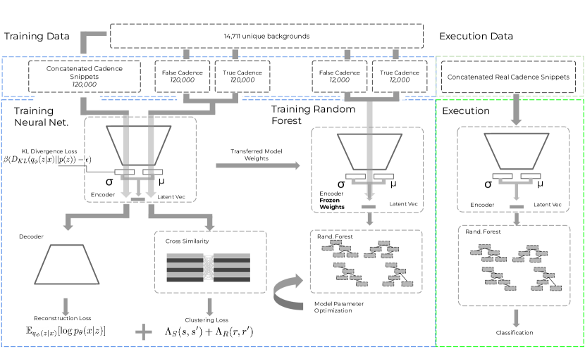
Refer to caption — Figure 1: Model training and execution scheme. Backward propagation of the neural network training is not shown for brevity.

The original VAE framework can be augmented with a single hyperparameter $\beta$ in the loss function that modulates the learning constraints applied to the model, specifically by controlling how much the model is penalized for how the model constructs the sample layer [14]. For our model we empirically select $\beta$ = 1.5 after comparing results from a number of validate sets, which appears to best help the model to learn disentangled features in the latent space. To further improve the model’s performance, we introduce an inductive bias where we assume that ETI signals have similar features in the ON’s and different features in the OFF’s [18]. We also assume that RFI will have similar features in all the OFF’s. This inductive bias is achieved by training the model to minimize or maximize an euclidean loss metric during training when presented with labeled data. Refer to the Methods section on Mathematical representations of the $\beta$ -VAE ML Architecture for further details on the mathematical representations of our model.

After constructing the $\beta-$ VAE we create a Random Forest classifier [19] to perform the classification. Random Forests use an ensemble of decision trees to build a classifier, with each tree acting as a vote of confidence. We employ a Random Forest in combination with our $\beta$ -VAE network because we needed to turn the encoder into a classifier and a Random Forest model is fast to train and execute. The greater the number of estimators (trees), the more robust a classifier is. We use the SciPy library⁴⁴4https://www.scipy.org with 1000 estimators and bootstrap it when constructing the individual trees. Empirically this gives the best run-time vs performance metric.

In order to train our ML algorithm and evaluate the model, we need to provide labelled data for the model to learn from. There are three main categories of labelled data that are relevant: (1) False data with no ETI signals, (2) True data with ETI signals, and (3) True data with ETI signals and RFI. Since we do not have a sample of real observational ETI signals for this purpose, we generate simulated events by artificially injecting signals into the input spectrograms using the Python package setigen⁵⁵5https://github.com/bbrzycki/setigen. A total of $14,711$ different snippets of backgrounds are used, obtained from three different cadences (see the Supplementary Tables. 1 and 2 for more details). This large sample of backgrounds should provide a good variety of scenarios to help the generalization of the training model. From these backgrounds, we randomly draw a heuristic 120,000 samples to form the training set. For (1), we use one quarter (30,000 samples) of the original backgrounds without injections, and an additional 30,000 samples with RFI injected to the backgrounds. Another 30,000 samples are labelled as (2), where we inject ETI signals into the backgrounds and are referred to as “True Single Shot” in this paper. Finally, the last 30,000 samples are labelled as (3), where we inject both ETI signals and RFI with a 1:1 relative intensity ratio into the background spectrograms. We have not simulated all combinations of intensity ratios since the model will, in principle, generalize this parameter. See Fig. 2 for an example of these three types of labelled data used. A caveat is that if a true, non-synthetic ETI signal is present in the original backgrounds, it would lead to a mislabelling of our training dataset. This is an unlikely scenario, and our large, 120,000-sample training set should minimize the effect of individual mislabelled data. Also note that we only train our model to detect signals that last for the entire cadence across the three ON scans. We do not attempt to assess the model’s performance towards intermittent ETI signals or signals that have a shorter span than the full cadence.

Another advantage of using simulated data is that we can control the injection parameters, namely the signal-to-noise ratio (S/N), the drift rate (DR) and the width ( $w$ ) of the signal. We set a range of 10 to 50 for the S/N and a DR of $\pm$ 8 Hz/s. Note that simulated ETI signals with zero drift rate are included. For $w$ , we choose a range where $\mathrm{DR}\times dt+5\leq w\leq\mathrm{DR}\times dt+55$ Hz, with $dt$ being the sampling rate. The lower bound offset of 5 Hz is chosen to be slightly wider than the amount of drift in one time bin at a given drift rate. This is necessary to prevent quantization of the injected signals as we do not have the native resolution in the filterbank-format observational data. Within the above ranges, we randomly draw a combination of S/N, drift rate and width for each simulated signal. See Supplementary Fig. 7 for the distribution of the final set of injected parameters.

In order to obtain the clustering loss matrix and the reconstruction loss vector, we need to train the encoder concurrently with concatenated (collapsed) cadences as well as non-collapsed cadences. We generate separate training sets for these to increase the diversity of the training set — that is, we have 120,000 samples of concatenated cadences as well as an independent 120,000 samples of false cadences and another 120,000 samples of true cadences. Refer to Fig. 1 for the breakdown of the size of the training set. The Random Forest model requires separate training since it needs to be built specific to a neural network where the weights are held constant. This is achieved by taking the outputs encoded by the $\beta$ -VAE and feeding the results into the Random Forest with synthetic labelled data. We create 12,000 false cadences and 12,000 true cadences (24,000 total) with the same breakdown ratio of various labelled categories. Overall, it takes roughly 12 hr to generate and train the full model with 100 iterations each time on our machines (see the Supplementary Figure 6 for further details on the specs of these computers).

Model Evaluation and Demonstration

We test our algorithm against traditional ML approaches, including a support vector machine (SVM) [20], a Random Forest [19], a classic, artificial neural network (ANN)[16], and a 3-D convolutional neural network (CNN)[16] in order to demonstrate its performance. The SVM and the Random Forest are both classifiers and can only work with feature vectors as input, so we perform an additional step of applying principal component analysis (PCA) on the unrolled feature vectors. We implement these models using the python module Scipy⁶⁶6https://www.scipy.org/ with further fine tuning discussed in sections "alternative model hyperparameter tuning" of the methods. A test bench of labelled data using different backgrounds were generated, which consists of 24,000 simulated snippets, with the same ratio of labelled events as our training set described earlier. The goal is to subject different ML models to this test bench and see how successful they are in recovering the correct signal classifications.

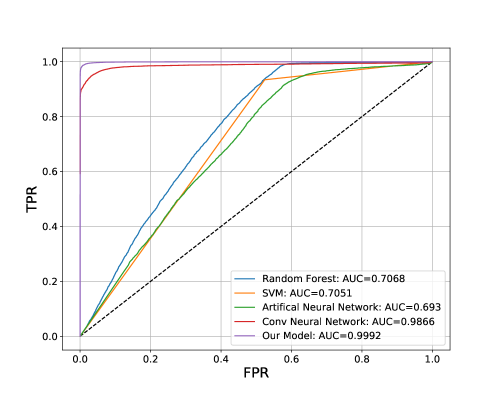
Fig. 3 shows a receiver operating characteristic (ROC) curve which evaluates the performance of each model at varying classification thresholds. All ML models perform well and are above the diagonal line. The Area Under the Curve (AUC) provides an aggregate measure of performance summing over all classification thresholds. A perfect model would have an AUC of 1. Our ML model has an AUC of 0.9993, a precision value of 0.993, a recall of 0.985 and an F1 score of 0.989. These are significantly higher than most of the other classical ML models, and marginally better than the second best model of the CNN. This provides evidence that simpler ML solutions perform less well than our $\beta$ -VAE-based model.

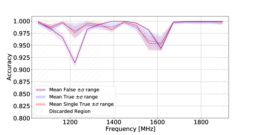
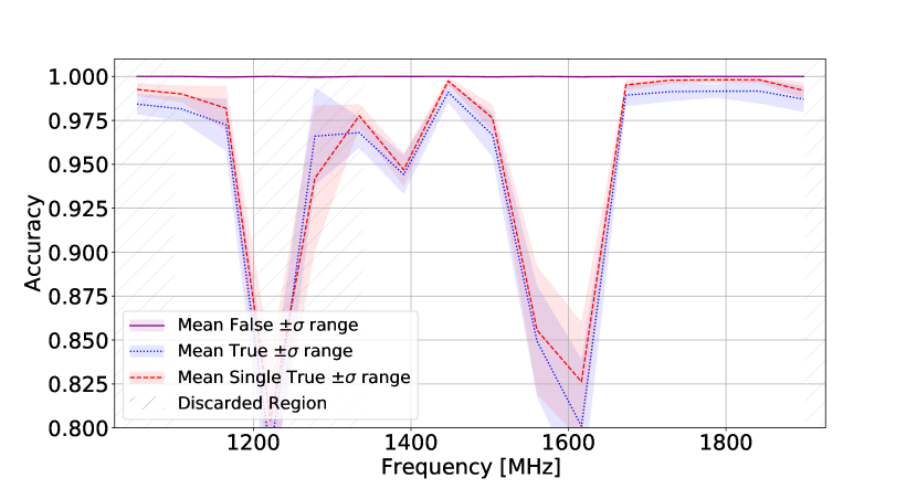
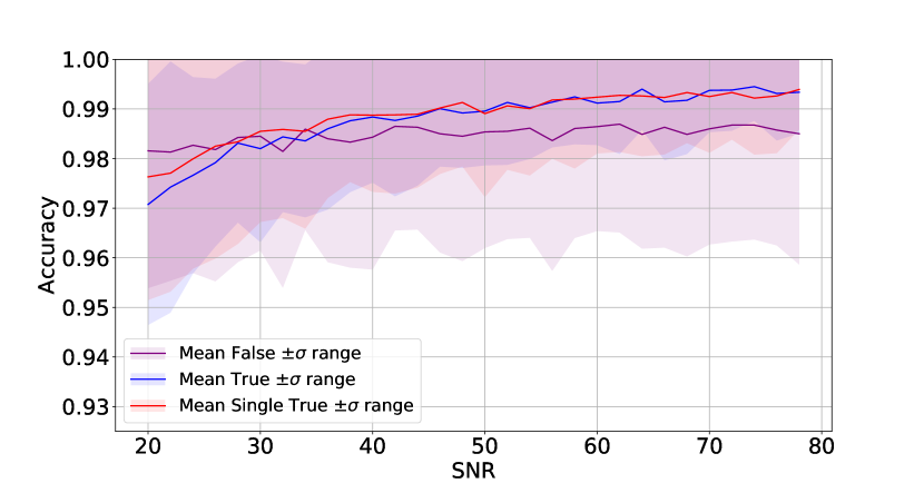
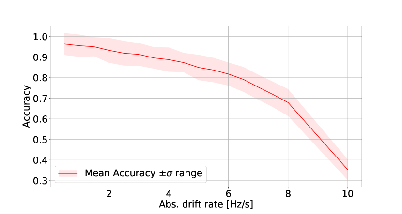
We also evaluate the model performance across the frequency band, the S/N and the drift rate ranges. From Supplementary Fig. 8a, we find that the overall accuracy is fairly high across the full band at a probability threshold of 50 $\%$ , with the majority of the sub-band having accuracy over 97.5%. In other words, False, Single True and Double True labelled data were correctly identified over 97.5% of the time. The few percent drop of accuracy near 1600 MHz corresponds to regions of the band that are heavily affected by RFI signals. As mentioned earlier, high false positive rate has been a persistent bottleneck in SETI efforts. Even a false positive rate of a few percent can translate to tens of thousands of candidates, reducing the search efficiency. We can attempt to drive down the false positive rate by selecting a higher classification threshold. As shown in Supplementary Fig. 8b, we find that at a threshold of 90%, we have a $<$ 1% false positive rate with a maximum 1- $\sigma$ uncertainty of $0.1\%$ . Naturally, a higher threshold will also mean worse true positive detection, meaning that we have a slightly higher chance of missing genuine ETI signals in the data. However, we see that the biggest drop in true positives happens in discarded regions of the band where prominent RFI is present. Barring those regions, we still have a true positive accuracy of above 95% in the rest of the band. For the S/N performance evaluation, we record a pretty consistent accuracy of $\gtrsim 95\%$ across S/N 20 to almost 80 (Supplementary Fig. 9a), with the largest uncertainty of $\pm 2.7\%$ per S/N bin. For the drift rate performance evaluation, we find that our performance drops as the drift rate increases (Supplementary Fig. 9b). At 8 Hz/s, we have roughly 70% accuracy in identifying “Single True” injected signals. This drops to about 35% at 10 Hz/s. This degradation can be explained by our unbalanced test samples (further discussed in the Methods section), where fewer high drift rate signals were employed in the training of the ML model.

Search Results

From the 115 million snippet windows searched, our ML model returns a total of 2,917,789 signals of interest. Small drift rate signal can potentially be seen by two adjacent overlapped snippets. Currently, each snippet is searched independently and we have not attempted to associate detections across them. Hence this 3 million signals of interest is likely an over count. We note that nearly 10% of these events came from a handful ( $\sim$ 1%) of cadences. These observations are heavily contaminated by RFI and skew the false positive rate of our analysis. We visualize the distribution of all events as a function of observing frequency as shown in Fig. 4. It can be seen that certain observing frequencies contain a much higher number of events compared to the others — for example the region around 1600 MHz. This overlaps with known RFI at the GBT site specifically from persistent GPS signals. Those regions of the spectrum are heavily contaminated by RFI and it would be challenging to detect anything apart from RFI in those frequencies. Indeed, from our performance assessment we see that our ML model is, by a few percent, slightly less accurate in these RFI-contaminated frequencies. Using the frequency histogram in the bottom left panel of Fig. 4 which has a histogram bin size of 4.97 MHz, we empirically determine a threshold to discard frequency bins with more than 35,000 events per bin, since this represents a conservative level where the main peaks of RFI clusters can be flagged. This equates to discarding 13 histogram bins, which is about 65 MHz of the entire band.

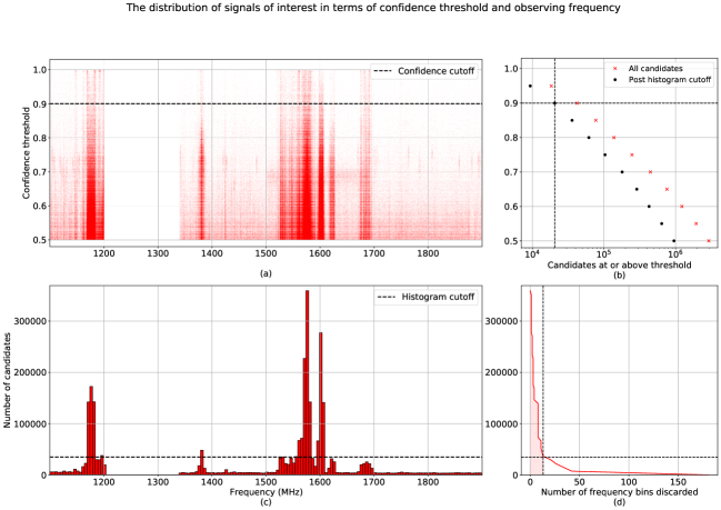
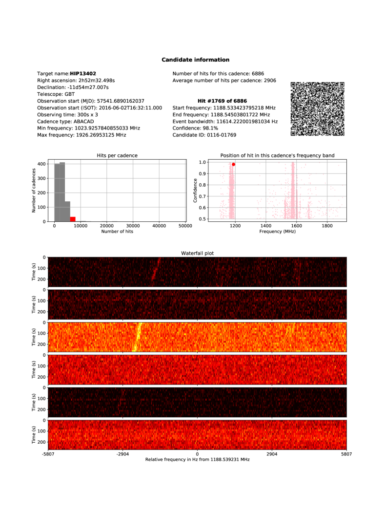
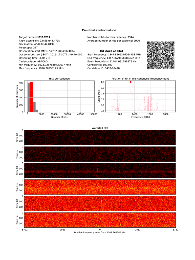
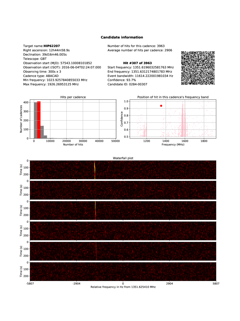
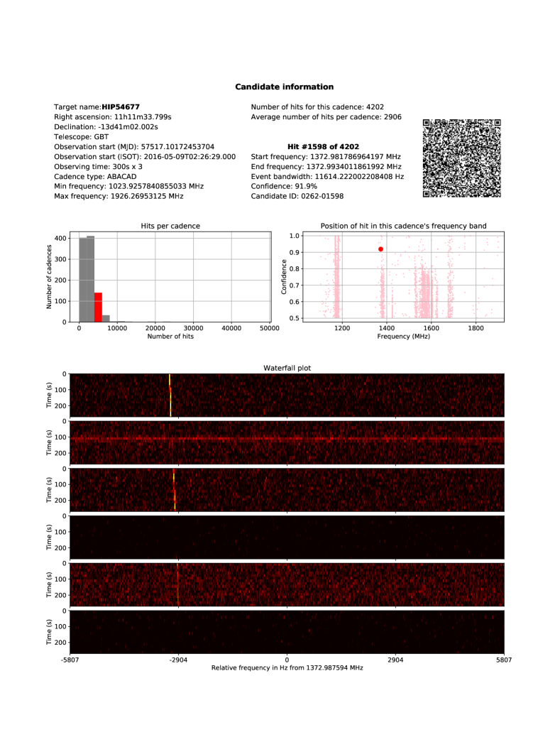
The top right panel of Fig. 4 shows the number of signals of interest at a range of classification thresholds, which has a quadratically increasing trend towards low thresholds. We further limit our signals of interest to those that have a classification threshold of over 90% in order to reduce the number of false positives. After applying these further filtering criteria, we are left with 20,515 signals of interest to assess. Upon a visual inspection, we identify $8$ promising signals of interest that show narrow, drifted signals in the three ON-scans (Fig. 5). Refer to Table 1 for their respective parameters. These $8$ signals of interest come from five different stars. HIP 13402 and 54677 both have spectral type K whereas HIP 62207 is a G star, HIP 56802 an F star and HIP 118212 is an M star. They are all within 30 to 90 ly from Earth. All five targets were analyzed by [3] and by [5] but they did not detect anything similar. Re-observations of these five sources took place on May 21, 2022, at the Green Bank Telescope using the same set up as the original observations. We analyze these data using the same $\beta$ -VAE pipeline and visually inspect all 72 events returned by the search. We do not detect anything like the $8$ signals of interest. This shows that no matter what the true nature of these signals are, they are not persistent in time. Given that the main goal of this work is to apply ML technique to identify signals with a specific pattern, we do not attempt to make a definite conclusion of whether these $8$ signals are genuinely produced by ETI. We encourage further re-observations of these targets.

We individually compute the drift rate and S/N of these signals of interest as they are not a by-product of our ML pipeline. We estimate the drift rate in each ON-scan separately using setigen. The uncertainty of the drift rate is defined to be the deviation of drift rates among the three ON scans. A number of interesting events were rejected despite showing narrow band drifted signals as we find that the drift rates across the three ON-scans are not consistent. We note that a changing drift rate does not necessarily mean the variation is non-physical. However, there is an infinite possibility of orbital motions that can phase connect three arbitrary drift rates. With a single dish SETI experiment, we have no independent way of verifying this and we consider it an intrinsic limitation of our search. We choose to exclude signals that are changing in drift rates for simplicity, as we cannot confidently relate them from one ON scan to the next. We also point out that MLc4 and MLc5 have the same drift rates and come from an observation of the same target, although at slightly different times and at different parts of the band.

ID	Target	Center Freq.	MJD	Confidence	Drift rate	S/N
		(MHz)			(Hz/s)
MLc1	HIP 13402	1188.539231	57541.68902	98.1	$+$ 1.11(25)	6.53
MLc2	HIP 118212	1347.862244	57752.78580	99.9	$-$ 0.44(7)	16.38
MLc3	HIP 62207	1351.625410	57543.08647	93.7	$-$ 0.05(10)	57.52
MLc4	HIP 54677	1372.987594	57517.08789	99.9	$-$ 0.11(3)	30.20
MLc5	HIP 54677	1376.988694	57517.09628	97.9	$-$ 0.11(2)	44.58
MLc6	HIP 56802	1435.940307	57522.13197	99.9	$-$ 0.18(4)	39.61
MLc7	HIP 13402	1487.482046	57544.51645	99.9	$+$ 0.10(2)	129.16
MLc8	HIP 62207	1724.972561	57543.10165	99.9	$-$ 0.126(10)	34.09

Table 1: The top

8

signals of interest identified by our ML model. We list the name of the ON-source target star, the frequency at the middle of the relevant

\sim

11 kHz snippet, the MJD of the detection, the topocentric drift rate, as well as the S/N of the signal. The HIP prefix in the source name shows that these targets are drawn from the Hipparcos catalog [21].

Regarding the nature of the rest of the events, most of them look like false positives associated with RFI signals. We have not exhaustively classified every single event and it is entirely possible that there are additional ETI-like signals that we have not picked up, including those that are too weak to be seen by human eyes. Other reasons as to why the false positive rate is higher than in our validation process include overfitting of backgrounds. The diversity of the RFI environment and the brightness of the RFI signals mean that it is unavoidable that our model would sometimes focus more on the background than the foreground signals. In addition, we do not have real ETI signals to train the model on, and instead have to rely on simulated signals that are injected to the sky backgrounds. Injection of signals might have altered the statistics of the snippets, introducing artefacts that were unintentionally learnt by the ML model.

Discussion

This work represents the most comprehensive ML-based technosignature search to date, and improves on previous work by finding signals of interest not detected before[3, 5]. We generate synthetic, labelled data to train a $\beta$ -VAE framework together with a Random Forest classifier. We observe some level of generalization in the trained model, as the latent space shows interpretable features and the model is able to correctly identify signals beyond the initial training parameter space.

Overall we see a high degree of accuracy when the model is subjected to a different test bench, both across the frequency band as well as over a wide range of signal S/N. Our model also performs better in comparison to a number of classical ML models tested.

By analyzing $1004$ cadences corresponding to approximately 115 million snippets recorded with the GBT 1.1–1.9 GHz receiver, our model returns 2.9 million events. Upon further filtering by discarding RFI affected frequency bins as well as by limiting the classification threshold to 90%, we further reduce the number of events to approximately 20,000. By visually inspecting the individual diagnostic plots, we discover $8$ promising SETI signals of interest with narrow band, drifted signals showing the expected on-off pattern that were not identified by previous turboSETI searches [3, 5]. We limit our search to drifting signals that have a uniform drift rate and are persistent across the three ON scans. However, a modified ML model can be adapted and re-trained to look for other ETI morphologies in the future, such as those with a spread spectrum emission. One main limitation of our ML implementation is that we have a non-uniform training set with fewer synthetic signals at higher drift rates (see Supplementary Fig. 7). This has likely skewed our model and misguided it that low drift rate events are more common.

Looking ahead, we hope to expand this ML technique to other Breakthrough Listen datasets to further increase the impact of ML on SETI. This includes other GBT and Parkes data, as well as the upcoming MeerKAT [22], Very Large Array (VLA)[23], Square Kilometre Array[24] and the next generation VLA (ngVLA; Ng et al., submitted) interferometric SETI projects.[25]

References

[1] Cocconi, G. & Morrison, P. Searching for Interstellar Communications. Nature 184, 844–846 (1959).
[2] Tarter, J. The Search for Extraterrestrial Intelligence (SETI). Annual Review of Astronomy and Astrophysics 39, 511–548 (2001).
[3] Enriquez, J. E. et al. The Breakthrough Listen Search for Intelligent Life: 1.1–1.9 GHz Observations of 692 Nearby Stars. ApJ 849, 104 (2017). URL https://doi.org/10.3847/1538-4357/aa8d1b. Publisher: American Astronomical Society.
[4] Price, D. C. et al. The Breakthrough Listen search for intelligent life: Wide-bandwidth digital instrumentation for the CSIRO Parkes 64-m telescope. Publications of the Astronomical Society of Australia 35 (2018). URL https://www.cambridge.org/core/journals/publications-of-the-astronomical-society-of-australia/article/breakthrough-listen-search-for-intelligent-life-widebandwidth-digital-instrumentation-for-the-csiro-parkes-64m-telescope/B7ABB2F93745A6677DD79BFAC96ACB98. Publisher: Cambridge University Press.
[5] Price, D. C. et al. The Breakthrough Listen Search for Intelligent Life: Observations of 1327 Nearby Stars Over 1.10-3.45 GHz. The Astronomical Journal 159, 86 (2020). 1906.07750.
[6] Price, D. C. et al. Expanded Capability of the Breakthrough Listen Parkes Data Recorder for Observations with the UWL Receiver. Research Notes of the American Astronomical Society 5, 114 (2021). URL https://ui.adsabs.harvard.edu/abs/2021RNAAS...5..114P. ADS Bibcode: 2021RNAAS…5..114P.
[7] Enriquez, E. & Price, D. turboSETI: Python-based SETI search algorithm (2019). 1906.006.
[8] Harp, G. R. et al. Machine Vision and Deep Learning for Classification of Radio SETI Signals. arXiv e-prints arXiv:1902.02426 (2019). 1902.02426.
[9] Zhang, Z.-S. et al. First SETI observations with china’s five-hundred-meter aperture spherical radio telescope (FAST). The Astrophysical Journal 891, 174 (2020). URL https://doi.org/10.3847/1538-4357/ab7376.
[10] Pinchuk, P. & Margot, J.-L. A machine learning–based direction-of-origin filter for the identification of radio frequency interference in the search for technosignatures. The Astronomical Journal 163, 76 (2022). URL https://doi.org/10.3847/1538-3881/ac426f.
[11] Czech, D., Mishra, A. & Inggs, M. A cnn and lstm-based approach to classifying transient radio frequency interference. Astronomy and Computing 25, 52–57 (2018). URL https://www.sciencedirect.com/science/article/pii/S2213133718300386.
[12] Zhang, Y. G., Won, K. H., Son, S. W., Siemion, A. & Croft, S. Self-supervised Anomaly Detection for Narrowband SETI. arXiv:1901.04636 [astro-ph] (2019). URL http://arxiv.org/abs/1901.04636. ArXiv: 1901.04636.
[13] Brzycki, B. et al. Narrow-band Signal Localization for SETI on Noisy Synthetic Spectrogram Data. Publications of the Astronomical Society of the Pacific 132, 114501 (2020). 2006.04362.
[14] Higgins, I. et al. $\beta$ -VAE: LEARNING BASIC VISUAL CONCEPTS WITH A CONSTRAINED VARIATIONAL FRAMEWORK. ICLR 2017 22 (2017).
[15] Kingma, D. P. & Welling, M. Auto-Encoding Variational Bayes. In 2nd International Conference on Learning Representations, ICLR 2014, Banff, AB, Canada, April 14-16, 2014, Conference Track Proceedings (2014). http://arxiv.org/abs/1312.6114v10.
[16] LeCun, Y., Haffner, P., Bottou, L. & Bengio, Y. Object Recognition with Gradient-Based Learning. In Forsyth, D. A., Mundy, J. L., di Gesú, V. & Cipolla, R. (eds.) Shape, Contour and Grouping in Computer Vision, Lecture Notes in Computer Science, 319–345 (Springer, Berlin, Heidelberg, 1999). URL https://doi.org/10.1007/3-540-46805-6_19.
[17] Snoek, J., Larochelle, H. & Adams, R. P. Practical bayesian optimization of machine learning algorithms. Advances in neural information processing systems 25 (2012).
[18] Mitchell, T. M. The need for biases in learning generalizations. Tech. Rep., Rutgers University, New Brunswick, NJ (1980). URL http://dml.cs.byu.edu/~cgc/docs/mldm_tools/Reading/Need%20for%20Bias.pdf.
[19] Breiman, L. Random Forests. Machine Learning 45, 5–32 (2001). URL https://doi.org/10.1023/A:1010933404324.
[20] Cristianini, N. & Ricci, E. Support Vector Machines. In Kao, M.-Y. (ed.) Encyclopedia of Algorithms, 928–932 (Springer US, Boston, MA, 2008). URL https://doi.org/10.1007/978-0-387-30162-4_415.
[21] Perryman, M. A. C. et al. The Hipparcos Catalogue. Astronomy and Astrophysics 500, 501–504 (1997).
[22] Czech, D. et al. The Breakthrough Listen Search for Intelligent Life: MeerKAT Target Selection. Publications of the Astronomical Society of the Pacific 133, 064502 (2021). 2103.16250.
[23] Hickish, J. et al. Commensal, Multi-user Observations with an Ethernet-based Jansky Very Large Array. In Bulletin of the American Astronomical Society, vol. 51, 269 (2019).
[24] Siemion, A. et al. Searching for extraterrestrial intelligence with the square kilometre array. In Proceedings of Advancing Astrophysics with the Square Kilometre Array — PoS(AASKA14) (Sissa Medialab, 2015). URL https://doi.org/10.22323/1.215.0116.
[25] Pinchuk, P. & Margot, J.-L. A machine learning–based direction-of-origin filter for the identification of radio frequency interference in the search for technosignatures. The Astronomical Journal 163, 76 (2022). URL https://dx.doi.org/10.3847/1538-3881/ac426f.
[26] Lebofsky, M. et al. The Breakthrough Listen Search for Intelligent Life: Public Data, Formats, Reduction, and Archiving. PASP 131, 124505 (2019). URL https://doi.org/10.1088/1538-3873/ab3e82. Publisher: IOP Publishing.
[27] Price, D., Enriquez, J., Chen, Y. & Siebert, M. Blimpy: Breakthrough Listen I/O Methods for Python. The Journal of Open Source Software 4, 1554 (2019).
[28] Sochat, V. Singularity Compose: Orchestration for Singularity Instances. JOSS 4, 1578 (2019). URL https://joss.theoj.org/papers/10.21105/joss.01578.
[29] Siemion, A. P. V. et al. A 1.1-1.9 GHz SETI Survey of the Kepler Field. I. A Search for Narrow-band Emission from Select Targets. The Astrophysical Journal 767, 94 (2013). 1302.0845.

Methods

The GBT 1.1–1.9 GHz dataset

We have chosen to deploy an ML SETI algorithm on the Breakthrough Listen GBT 1.1–1.9 GHz dataset, sourced from several different observational campaigns, as it is one of the largest homogeneous SETI datasets available in a single location at the Berkeley SETI Research Center. The majority of this dataset has been made publicly available⁷⁷7https://seti.berkeley.edu/opendata. The dataset used in this work has a frequency range of 1023 $-$ 1926 MHz and consists of a total of $1004$ cadences from $820$ unique targets observed over 480 hr. In total, $\sim 120$ TB of data has been analyzed in this work.

Each cadence has six 4.8-min observations recorded in HDF5 format. In the analysis described here, we exclusively work with the fine-frequency resolution data[26]. More than half of the cadences have a frequency resolution of 2.79 Hz and 322,961,408 frequency channels. The remaining 397 cadences taken before 2016 April have a frequency resolution of 2.84 Hz and 318,230,528 channels per observation. All data have a time resolution of $\sim$ 18 s and 16 time bins for each observation within the cadence. Parts of the band are affected by instrumental artifacts, including steep roll-off on the band edges and at the boundaries of an analog notch filter. These regions are at frequencies $\nu<$ 1.1 GHz, $\nu>$ 1.9 GHz and 1.2 $<\nu<$ 1.34 GHz. Together these equate to about 30% of the full band and are excluded from our search.

Two types of cadences have been used in the GBT observations, the ABACAD pattern and the ABABAB pattern. The difference between these is that the “ON-source” scans (the A scans) can be interspersed with identical “OFF-source” targets (the B scans) or three different “OFF-source” targets (B, C, D). In both cases, the minimum angular offset between ON and OFF source scans is at least six beamwidths, which is well beyond the primary and side lobes of the GBT beams. In fact, the majority (over 80%) of the cadences analyzed have an angular offset of as much as 38 beamwidths. We treat both types of cadences the same way in our analysis, since for the purpose of spatial filtering we only care that the “OFF-scans” are sufficiently far from the “ON-scans”.

In our simulated data, we have assumed no time delay between the six observations in a cadence, although in reality, there is a small amount of slew time switching between ON and OFF scans. We have discarded cadences that have a long ( $\geq$ 2 min) pause between the individual observations, since that would significantly alter the data characteristics due to longer term variation in telescope performance and our ML model has not been trained to detect those. The $1004$ analyzed have typically a small time gap of the order of a minute and we have effectively assumed the observations are continuous for simplicity. For signals with a low drift rate of say 1 Hz/s, this is not really an issue, since a minute of time delay would correspond to a shift of about 60 Hz which is only 2 or 3 frequency bins in the downsampled snippet used for the ML search. However, this issue becomes more prominent at high drift rates. For example, at the maximum detectable drift rate of 10 Hz/s, during the minute of gap the signal would have shifted by about 600 Hz, which is roughly 25 downsampled frequency bins. We note that it is an oversight on our part, as not taking time delay into account could have affected our ability in detecting signals with high drift rates.

Data preprocessing

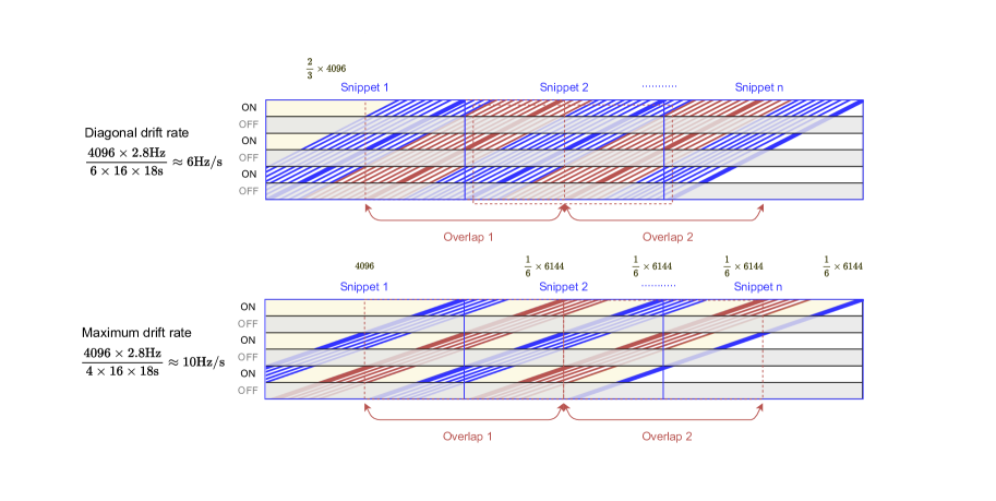
Neural networks perform better if the input data has a shape close to that of a CNN kernel which typically has a 1:1 aspect ratio. In contrast, the fine-resolution GBT data have a very elongated dimension, with over 300 million frequency bins by 16 time bins per observation. Indexing small partitions of the frequency band and searching them independently can solve that problem, but a small frequency band will reduce the maximum drift rates our algorithm is sensitive to, since the algorithm cannot detect any signal that drifts beyond the diagonal of the input data shape. Here we define the maximum drift rate detectable by a search to be when a signal starts drifting from the corner of the first observation and drift out near the opposite corner of the third ON scan, spanning a total of four observations (ON-OFF-ON-OFF) worth of time (see bottom panel of Supplementary Fig. 6a).

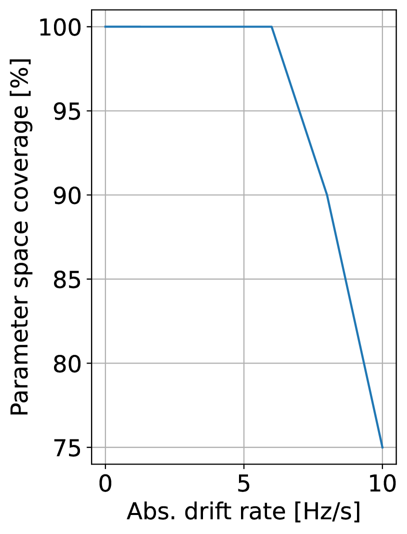
We find a good compromise in using snippets of 4096 frequency bins, which provides sensitivity to a maximum drift rate of 4096 $\times$ 2.8 Hz over 16 $\times$ 18 s per observation over 4 observations $\approx\pm$ 10 Hz/s. These higher drift rates have a proportionally higher chance to drift out of at least one of the snippets depending on where the signals start, partially altering the expected ON-OFF pattern and reducing the sensitivity of our model towards these cases. In order to alleviate this potential issue, we devise an overlapping search that will cover snippets offset by 2048 frequency bins which is half the size of a snippet window (Supplementary Fig. 6). In the scheme illustrated in the top panel of Supplementary Fig. 6a, any drift rate lower than the diagonal drift rate, i.e. 4096 $\times$ 2.8 Hz/(6 $\times$ 16 $\times$ 18 s) $\approx$ 6 Hz/s will either be detectable by the blue snippets or by the red overlap search. Only a very small yellow-highlighted region on the far left is missed since too much of the drifting signals happen before the start of the snippet. Compared to the large number of snippets per cadence, this equates to a 99.999% of parameter space coverage. For signals with higher drift rates than the diagonal, the overlap search would not be quite enough to fully cover some of the parameter space. The bottom panel of Supplementary Fig. 6a shows the most extreme case at the maximum detectable drift rate of 10 Hz/s. At this point, apart from a slightly larger triangle on the left that will be missed, there are now gaps between the blue and the red drifting signals that we are not sensitive to. The probability of having the signal detectable within a cadence drops to $\sim$ 75 % at $\pm$ 10 Hz/s (Supplementary Fig. 6b).

We further downsample the snippets in frequency by a factor of 8 (to a frequency resolution of 22.32 Hz or 22.72 Hz) by averaging every 8 pixels. This results in an input spectrogram with shape [time, frequency]=[16, 512]. This helps to further improve the training time and performance of the neural network, at the expense of decreasing the S/N of a potential signal contained in one channel by $\sqrt{8}$ .

The dynamic range of these GBT data can vary by as much as a factor of $10^{11}$ , as a result of the long Fast Fourier Transform (FFT) used to generate these high spectral resolution data. After the injection stage, we log normalize the data, shift everything to be positive and we scale the data to have a final range within 0 and 1. Note that the normalization is done per snippet of each cadence and not across the entire cadence.

Drift rate range trained

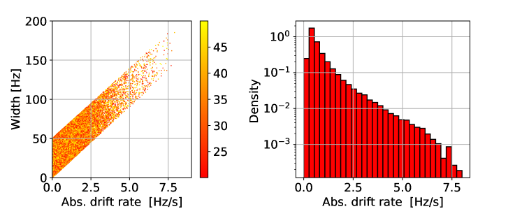
Within the S/N, width, and drift range ranges specified in Table 2, we randomly draw a combination of S/N, drift rate and width for each simulated signal. See Supplementary Fig. 7 for the distribution of the final set of injected parameters. Note that there are fewer simulated signals at higher drift rates. This is partly because there is a higher chance for them to drift out of our detectable parameter space as can be seen in Supplementary Fig. 6, and also because we have not simulated signals that start outside of a snippet but drift into it. Supplementary Fig. 7b shows the density distribution of our simulated sample as a function of drift rate. To quantify the overall detectability of this ML model as a function of drift rate, we should take into account both the parameter coverage as provided by the overlap search (right panel of Supplementary Fig. 6), as well as the sampling distribution of simulated data (right panel of Supplementary Fig. 7). We estimate that we have a $\sim$ 80% sensitivity towards a 6 Hz/s signal that was present in this dataset, a $\sim$ 60% sensitivity towards an 8 Hz/s signal and a $\sim$ 25% sensitivity towards a 10 Hz/s signal. The fact that we do not have a balanced test class with respect to drift rate means our model is less well-trained for the high-drift region of the parameter space.

Mathematical representations of the $\beta$ -VAE ML Architecture

In this analysis, we use a VAE-based ML model [15], which is one of two main families of deep generative models that can produce highly realistic versions of the input data. Autoencoders are neural networks architectures with an encoder and a decoder that form a bottleneck for the data to go through. They are trained to minimize the loss of information during the encoding-decoding process, which is achieved by iterations of gradient descent with the goal of diminishing the reconstruction error. A VAE is a special kind of autoencoder whose encoding distribution is regularized. The term “variational” reflects the relationship between the regularization and the variational inference method in statistics. A mathematical representation of our model is shown by Equation 1, which is a slightly modified version of Equation 3 in [15]. In the referenced paper, $\mathcal{L}$ was used to represent the Lagrangian. Here we flip the sign of the equation to show the loss function $L$ as follow:

L(\theta,\phi,\beta;x,z)=\overbrace{-\mathbb{E}_{q_{\phi}(z|x)}[\log p_{\theta}(x|z)]}^{\mathrm{Reconstruction\leavevmode\nobreak\ Loss}}+\overbrace{\beta(D_{\mathrm{KL}}(q_{\phi}(z|x)||p(z)))}^{\mathrm{KL\leavevmode\nobreak\ Divergence}}.\centering\@add@centering

(1)

In this Equation, $x$ is the observational data and we want to develop an unsupervised deep generative model which will learn the joint distribution of the data $x$ and a set of generative latent factors $z$ . This effectively is the probabilistic decoder, $p_{\theta}(x|z)$ , with generative model parameters $\theta$ , where for a given $z$ it produces a distribution over the possible corresponding values of $x$ . Inversely, $q_{\phi}(z|x)$ is the probabilistic encoder with recognition model parameters $\phi$ , where for a given data point $x$ it produces a distribution over the possible values of $z$ from which the data point $x$ could have been generated. $\mathbb{E}_{q_{\phi}(z|x)}$ computes the (log-)likelihood of effectively each pixel that the model reconstructs. The function $D_{KL}$ is the Kulback-Leibler (KL) Divergence. To summarize, the two main terms in this Equation are the reconstruction loss and the $\beta$ -weighted Kulback-Leibler (KL) divergence. The KL divergence metric is used to measure the statistical similarities between the mean and the log-normalized standard deviation layers.

Specifically for our analysis, we also want the model to be able to group observations with similar features together in the model’s latent space. In order to achieve this we incorporate a clustering loss which we denote $\Lambda$ . We use $\Lambda_{\mathrm{S}}$ for SETI and $\Lambda_{\mathrm{R}}$ for RFI signals. We compute the latent vectors of the cadence for true SETI cases called $S$ with corresponding latent factor $s^{\prime}$ and an input of $s$ . Similarly, we label the corresponding parameters for false SETI cases (RFI) as $R$ with corresponding latent factor $r^{\prime}$ and an input of $r$ :

S=q_{\phi}(s^{\prime}|s)\,,\quad R=q_{\phi}(r^{\prime}|r)\,.

(2)

Each parameter represents a set of six feature vectors corresponding to the six observations each encoded from the cadence. We define two lists to index each vector in the set of features as follow:

\text{ON}=\{0,2,4\}\,,\quad\text{OFF}=\{1,3,5\}\,.

(3)

We compute the distance between each encoded feature vector on the true SETI cadence we have for every pair of ON targets (3 $\times$ 2 different combinations) and pair of OFF targets (another 3 $\times$ 2 different combinations). We compute their similarities, whereas for a pair of adjacent ON-OFF (3 $\times$ 3 different combinations) we compute the inverse. The indices $i$ and $j$ represent the ID of the observation and each goes from 0 to 5. The only condition is that $i\neq j$ . We then average over $n=21$ combinations to get the clustering losses:

\Lambda_{S}=\frac{1}{n}(\sum_{i\in\text{ON}}\sum_{\begin{subarray}{c}j\in\text{ON}\end{subarray}}||S_{i}-S_{j}||^{2}+\sum_{i\in\text{OFF}}\sum_{\begin{subarray}{c}j\in\text{OFF}\end{subarray}}||S_{i}-S_{j}||^{2}+\sum_{i\in\text{ON}}\sum_{j\in\text{OFF}}\frac{1}{||S_{i}-S_{j}||^{2}})\,.

(4)

For the false SETI (RFI) cadence, since we inject a continuous signal across all six observations, we can assume that every pair of observations will look similar. Therefore, we compute the distance between each encoded feature vector for the RFI cadence by calculating the similarity between every pair and average over them to get the clustering losses:

\Lambda_{R}=\frac{1}{n}(\sum_{i\in\text{ON}}\sum_{\begin{subarray}{c}j\in\text{ON}\end{subarray}}||R_{i}-R_{j}||^{2}+\sum_{i\in\text{OFF}}\sum_{\begin{subarray}{c}j\in\text{OFF}\\ \end{subarray}}||R_{i}-R_{j}||^{2}+\sum_{i\in\text{ON}}\sum_{j\in\text{OFF}}||R_{i}-R_{j}||^{2})\,.

(5)

A smaller $\Lambda_{S}$ implies that all the ON targets have vectors that are close together and all the OFF targets are close together, whereas the ONs and OFFs are far apart. This is in contrast to a smaller $\Lambda_{R}$ where all the signals are close to each other. In other words, we can identify true ETI signals this way because the ON scans (A) will be separated furthest from the rest of the OFF scans (B, C, D).

By formulating the cost function in this manner, we help the neural network to make an “implicit” classification that groups relevant features together. Finally we include another hyperparameter weight $\alpha$ to tune the relative “importance” of the loss metric. We empirically set $\alpha=10$ as it gave the best performing model. In summary, the loss function ( $L$ ) of our model can be represented by:

L(\theta,\phi,\beta;x,z,s,r)=\overbrace{-\mathbb{E}_{q_{\phi}(z|x)}[\log p_{\theta}(x|z)]}^{\text{Reconstruction Loss}}+\overbrace{\beta(D_{KL}(q_{\phi}(z|x)||p(z)))}^{\text{KL Divergence }}+\alpha\overbrace{(\Lambda_{S}(s,s^{\prime})}^{\text{SETI }}+\overbrace{\Lambda_{R}(r,r^{\prime})}^{\text{RFI }})\,.

(6)

Backgrounds used for the Training Data and Test Benches

For the training data, a total of $14,711$ different snippets of backgrounds are used, obtained from three different cadences (see Supplementary Table 2). These backgrounds are taken from regions of the band (1418.7 to 1587.9 MHz) that overall showed higher than average RFI as determined by the previous turboSETI search [3], which we can confirm by visually inspecting these regions in the three cadences. The intention is that our model is trained with some examples of the most RFI-contaminated observations. A more rigorous selection of backgrounds could be achieved by identifying snippets with statistical anomalies in energy, as well as by employing a larger number of cadences to increase the diversity in the backgrounds. However, we believe that our large sample of backgrounds should provide a good variety of scenarios to help the generalization of the training model.

Training target	Cadence	Freq range	Bandwidth	Freq. res	No. of snippets	No. of test samples
		(MHz)	(MHz)	(Hz)
$\beta$ -VAE	HIP 110750	1418.7 $-$ 1475.1	56.4	2.79	4928	120,000
	HIP 13402	1475.1 $-$ 1531.5	56.4	2.83	4855
	HIP 8497	1531.5 $-$ 1587.9	56.4	2.79	4928
Random Forest	HIP 110750	1418.7 $-$ 1475.1	57.139	2.79	4928	24,000

Table 2: The breakdown of the number of background snippets and the frequency ranges of each cadence used for the training dataset. The number of test samples simulated in each training set is also listed.

In order to evaluate the model performance, we generate different test benches of labelled data. Supplementary Table 3 summarizes the properties of these test sets. For the test where we compare our $\beta$ -VAE model with other ML models, we create a test bench that consists of an RFI-free band (1418.7 $-$ 1475.1 MHz) of a new observation of HIP15638 that our model has not seen before, as well as an RFIaffected band (1644.5 $-$ 1700.7 MHz) from HIP 13402. 24,000 samples are drawn, with the same ratio of labelled events as our training set, i.e. half False data, a quarter “True Single Shot” and a quarter “True Double Shot”. The goal is to subject different ML models to this test bench and see how successful they are in recovering the correct signal classifications.

In order to evaluate the model performance across the frequency band and across the S/N range, we create one test bench using an observation of HIP 15638 as the background. We split the full GBT data into 16 sub-bands and we step through the S/N range of 20 to 80 with a step size of 2, resulting in 30 S/N bins. We deliberately simulate signals brighter than the max S/N of 50 used in the initial training dataset. The idea is to see if our model has successfully generalized to high S/N signals that it was not previously trained on. For each frequency sub-band and each S/N bin, we simulate 1000 test samples. This amounts to a total of 16 $\times$ 30 $\times$ 1000=48,0000 simulated signals, again with the same ratio of labelled events and same ranges of widths and drift rates as our training set.

For the frequency test, we average over all S/N and compare across the 16 sub-bands. Since our test bench consists of balanced data, i.e., an equal amount of False and True signals, we show the performance at the standard probability threshold of $50\%$ in Supplementary Fig. 8a and we consider a more stringent classification threshold of $90\%$ in Supplementary Fig. 8b. For the S/N test, we average over all frequency sub-bands and compare across the 30 S/N bins in Supplementary Fig. 9a.

For the drift rate performance evaluation, we simulate “Single True” signals between a drift rate range of 0.5 to 10 Hz/s with a step size of 0.5 Hz/s. At each drift rate, we loop through the 16 sub-bands each with 1000 samples of randomly selected S/N within the range of 20 $-$ 80. This sums to a total of 16,000 samples per drift rate and the result can be seen in Supplementary Fig. 9b.

Test type	Source	Freq range	N. Bgs	N. Tests	S/N range	N_bin S/N	$\mid$ DR $\mid$	N_bin DR
		(MHz)					(Hz/s)
Other models	HIP 15638	1418.7 $-$ 1475.1	4928	24000	20 $-$ 80	30	0 $-$ 8	n/a
Other models	HIP 13402	1644.5 $-$ 1700.7	4928	24000	20 $-$ 80	30	0 $-$ 8	n/a
Full-band &	HIP 15638	1023.9 $-$ 1926.3	78848	480000	20 $-$ 80	30	0 $-$ 8	n/a
S/N	HIP 15638	1023.9 $-$ 1926.3	78848	480000	20 $-$ 80	30	0 $-$ 8	n/a
Drift rate	HIP 15638	1023.9 $-$ 1926.3	78848	320000	20 $-$ 80	n/a	0.5 $-$ 10	20
Latent Space	HIP 110750	1531.5 $-$ 1587.9	4928	4928	n/a	n/a	n/a	n/a

Table 3: Summary of the simulated data parameters for the test benches. We list the test type for each test bench. The source name of the cadence and the frequency range used are shown. The corresponding number of unique background snippets (N. Bgs) is listed, from which we randomly draw the said number of test samples (N. Tests) to inject simulated signals. The S/N range for each case is shown as well as the number of S/N bins evenly distributed within the range — except when the S/N are randomly chosen from the range specified we denote the cell with “n/a”. Similarly, we list the absolute value of drift rate (DR) and its number of bins. For the latent space test, no simulated signal is injected.

Alternative Model Hyperparameter Tuning

Four alternative ML models were considered for this SETI project, namely Random Forest, SVM, ANN, and CNN. We conduct a large-scale hyperparameter search in order to find the best configurations for each model. We search 1000 different variations for Random Forest and SVM. For the ANN and CNN, we search 3000 variations and each time train with 100 epochs. Using a Bayesian optimization technique, we sample a total of 128 variations out of all these possibilities, executed on a $k$ -fold cross validation set with 5 splits. In other words, a total of 640 variations were trained. Parameters that have led to the best performing models are highlighted in bold in Table 4. The averaged and best AUC from this search can be found in Table 5. The averaged AUCs all have very small standard deviations, which is to say that the performance of each of these four models are pretty consistent across the hyperparameter space searched, and only marginal improvement has been achieved by fine tuning the hyperparameters over the default, ‘out-of-the-box’ configurations. Note that these AUCs are results of the hyperparameter search using the validation data set, which are not the same as the AUCs listed in Table 6 from the test data. The AUCs from the hyperparameter search appear to be a little higher than those from the test data. This is expected as some degree of overfitting can happen when optimizing on the validation set.

Random forest
Parameters	Values
Number of estimators	10, 50, 100, 200, 500, 1000
Parameter criterion	gini, entropy
Maximum depth	5, 10, 20, 30, None
Maximum features	auto, sqrt, log2
SVM
Parameters	Values
C regularization	0, $1\times 10^{-6}$ , 1, 2, 10, 50, 100
Degree	1, 2, 3, 5, 7, 9
Kernels	linear, poly, rbf, sigmoid
Artificial neural net
Parameters	Values
First layer weights	256, 512
Number of first layers	1, 2
Activations for the first layers	ReLU, sigmoid
Second layer weights	128, 256
Number of second layers	1, 2
Activations for the second layers	ReLU, sigmoid
Third layer weights	32, 64
Number of third layers	1, 2
Activations for the third layers	ReLU, sigmoid
Final activation	sigmoid, softmax
Learning rate	0.001, 0.0001, 0.00001
Convolutional neural net
Parameters	Values
First-layer filter size	8, 16, 24
Number of first layers	1, 2, 3
Activations for the first layers	ReLU, sigmoid
Second-layer filter size	32, 64, 128
Number of second layers	1, 2, 3
Activations for the second layers	ReLU, sigmoid
Third-layer filter size	64, 128
Number of third layers	1, 2, 3
Activations for the third layers	ReLU, sigmoid
Hidden layer weights	256, 128
Final activation	sigmoid, softmax
Learning rate	0.001, 0.0001, 0.00001

Table 4: Parameter values searched for each of the four sets of alternative models. The values in bold indicate the best performing model.

Model	N. variations	Averaged AUC	Best AUC
Random Forest	1000	0.77(1)	0.79
SVM	1000	0.72(9)	0.78
ANN	3000	0.73(1)	0.74
CNN	3000	0.95(2)	0.98

Table 5: The number of variations of parameter values searched, the averaged AUCs with standard deviation shown in brackets, as well as the best AUCs of the four alternative ML models from the hyperparameter tuning using the validation data set.

Further details on the Performance Assessments

For the benchmark test against other ML models, we compute the standard metrics of precision, recall and F1 scores as recorded in Supplementary Table 6. Precision describes how well the positive labels are determined, and is defined by the number of true positives (TP) divided by the number of true positives plus false positives (TP+FP). Recall is defined as TP divided by the total positive samples (true positives plus false negatives; TP+FN). The F1 score is a measure of both of those metrics, where F1=2 $\times$ (Recall $\times$ Precision) / (Recall + Precision). Supplementary Figs. 8 and 9 show our model accuracy as a function of the observing frequency, S/N and drift rate.

Model	Best AUC	Precision	Recall	F1
Random Forest	0.7123	0.641	0.956	0.767
SVM	0.7115	0.643	0.951	0.767
ANN	0.6768	0.636	0.659	0.647
CNN	0.9817	0.992	0.934	0.959
Our Model	0.9993	0.994	0.985	0.989

Table 6: The best AUCs, precision, recall, and F1 scores of the five ML models applied on the test data set.

Latent Space Analysis

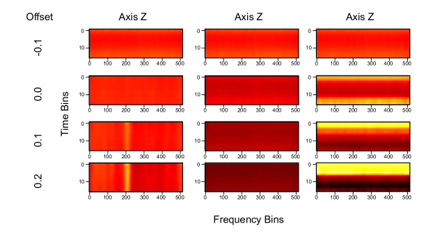
In order to understand and interpret how our ML algorithm makes classification decisions, we study the latent space of the decoder with the goal of finding out whether the network is able to disentangle each of the learned features. The first three axes appear to produce human interpretable results and so we further study their feature vectors and we perturb each axis in steps of 0.1. These variations are then fed back into the decoder and we visualize the resultant spectrograms in Supplementary Fig. 10. Axis $z$ 1 looks to have encoded the feature of S/N as perturbing this axis creates a brighter signal. Axis $z$ 2 appears to represent the level of background noise and axis $z$ 3 corresponds to instrumental artifacts which are commonly seen as bright horizontal bands across part of the spectrum. We interpret this outcome as evidence that the network has learnt relevant features from the dataset, helping it make the right decisions during the classification stage.

To quantify this performance, we implement a disentanglement metric [14] by simulating idealized signals with four axes of latent space vectors, namely drift rate, width of the signal, SNR and frequency. We then applying a linear classifier on the latent space vectors to differentiate between different perturbations of simulation parameters. If disentanglement is successful, a linear classifier is sufficient in separating changes in the four axes just from the latent vectors. The accuracy of the benchmark $\beta$ -VAE from [14] achieved a maximum accuracy of 99.2% where as the traditional VAE had only 61.6%. Our model returns an accuracy of 70.1%, which is superior compared to that of a traditional VAE model and confirming our improvement in disentanglement and interpretability scores. The drop in disentanglement score in respect to the $\beta$ -VAE is due to the fact that our model used a smaller $\beta=1.5$ factor rather than $\beta=4$ factor from the original implementation. This difference in factors was to balance the custom loss function we constructed for the cadence clustering.

Search Pipeline

We develop a processing pipeline in order to systematically analyze the 120 TB of GBT 1.1–1.9 GHz data. Within each 4096-channel snippet, each search is completely independent and hence can be easily parallelized. We have access to three compute nodes at the Berkeley data centre for this analysis (see Supplementary Table 7 for the hardware specifications), therefore we divide up the dataset into three equal sub-sets to run on the three machines independently as shown in Supplementary Fig. 11. On each machine, we launch five parallel instances of the processing that independently work on different cadences. The status of the processing on each machine is monitored and managed manually.

Initially, we divide up the full frequency band into 16 sub-bands. This allows us to load observations faster into memory compared to reading in and processing each 4096-channel snippet one by one, because of the switching cost during input/output (I/O) vs processing. The I/O was done using the python package Blimpy⁸⁸8https://github.com/UCBerkeleySETI/blimpy as described in [27]. We concatenate the six observations of a cadence before feeding it into the neural network, which is built using the Tensorflow API and is GPU-accelerated. Furthermore we distribute the training across multiple GPUs implementing a typical asynchronous mirrored approach. Because we mirror each model on different GPUs we can afford to execute the model on batch sizes of $10^{4}$ snippets given the GPU memory constraints to further parallelize execution. Finally the features are fed into the Random Forest classifier which runs in parallel on the CPU.

The search pipeline, disregarding I/O, takes $<$ 5 s to search $1/16^{\mathrm{th}}$ of the band. The I/O and the preprocessing take the most amount of compute time despite it being implemented to compute in parallel and with just-in-time compilers (JIT) such as NUMBA⁹⁹9https://numba.pydata.org/, taking $50-60$ s to run on the same $1/16^{\mathrm{th}}$ band. The search time on a single 30 min cadence is $18.7\pm 1.6$ min. The variation is mostly due to cache preloading for some data. However the runtime of the core of the search pipeline disregarding the I/O stays relatively constant from cadence to cadence.

We achieve further speed-up via a custom container orchestration using Singularity¹⁰¹⁰10https://sylabs.io/ and the schematic is shown in Supplementary Fig. 11. By running multiple instances of the same search on smaller subsystems on the same compute node, it scales faster in practice than running a single instance on all the resources [28]. This is because each search is completely independent from each other and hence does not require sharing memory or data. This is far more efficient than parallelizing individual operations such as I/O where data needs to then be recombined together.

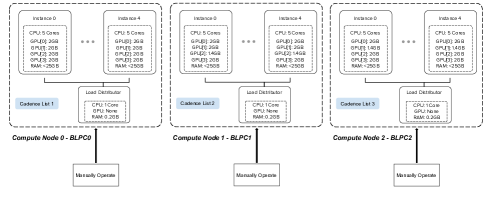
	Compute Node 0	Compute Node 1	Compute Node 2
CPU	Intel Xeon E5-2630	Intel Xeon E5-2630	Intel Xeon Silver 4210
GPU[0]	NVIDIA TITAN X	NVIDIA TITAN X	NVIDIA TITAN X
GPU[1]	NVIDIA TITAN X	NVIDIA TITAN XP	NVIDIA GTX 1080
GPU[2]	NVIDIA TITAN X	NVIDIA GTX 1080	NVIDIA GTX 1080 Ti
GPU[3]	NVIDIA TITAN X	NVIDIA TITAN XP	NVIDIA GTX 1080 Ti
RAM	256 GB	256 GB	196 GB

Table 7: The hardware specifications for each compute node used in this analysis.

Signal of interest visualization

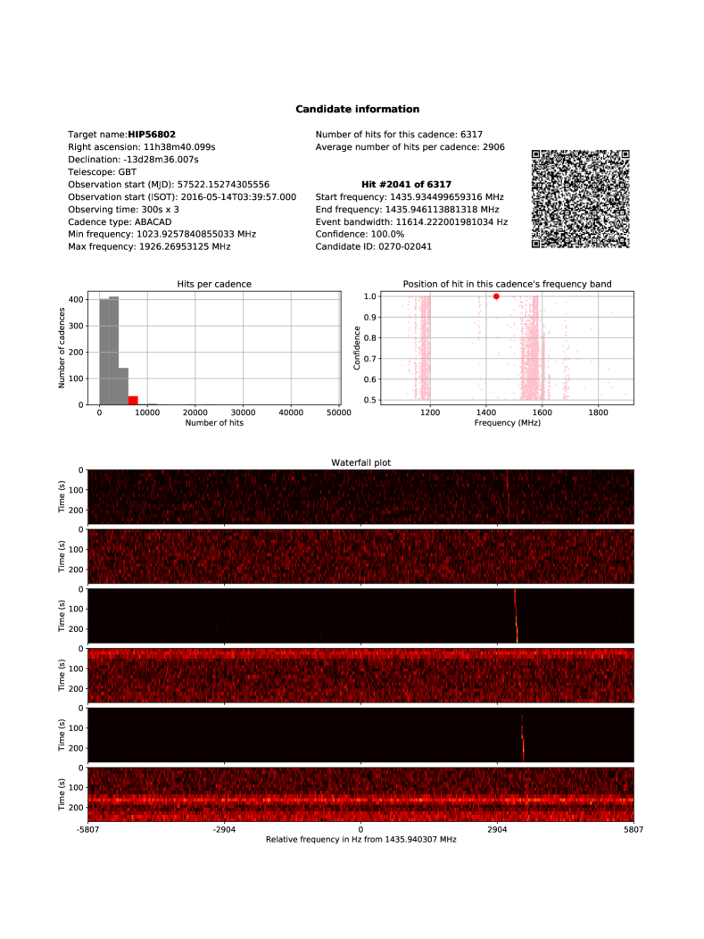
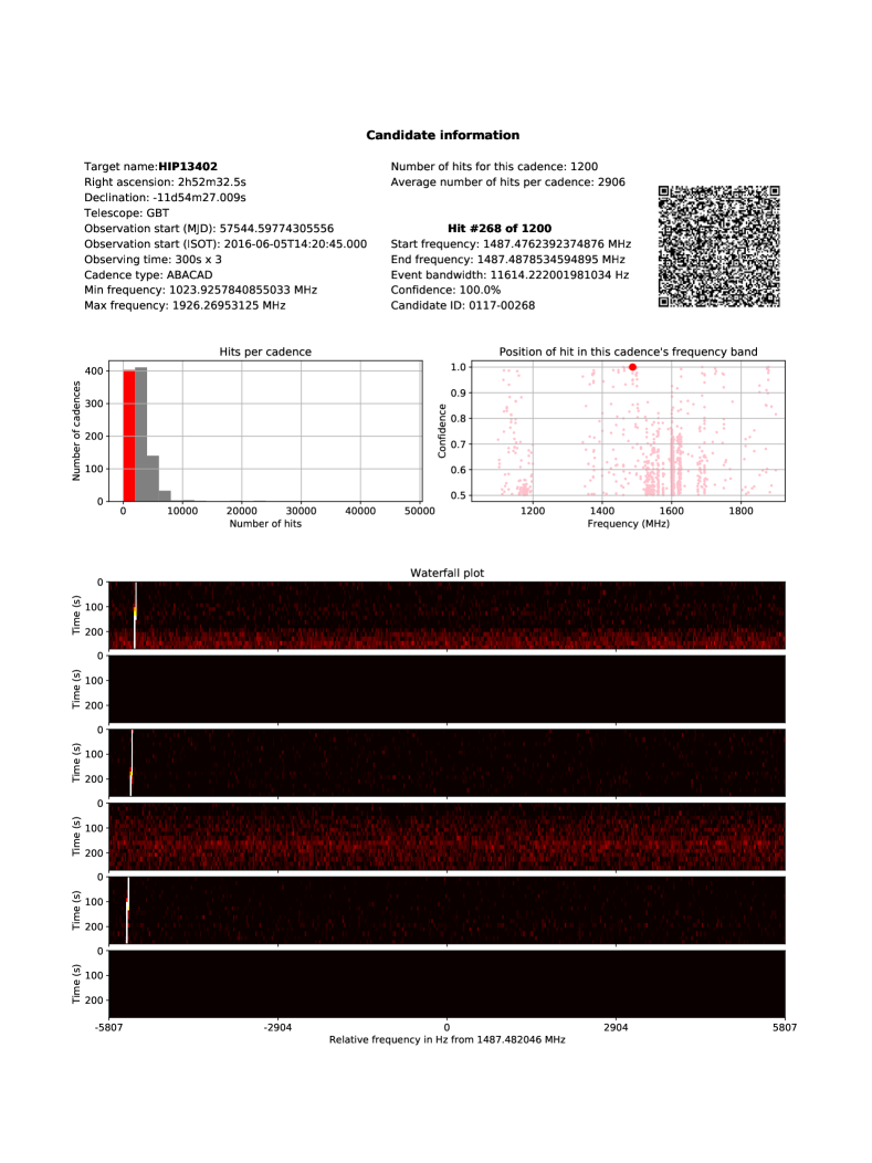
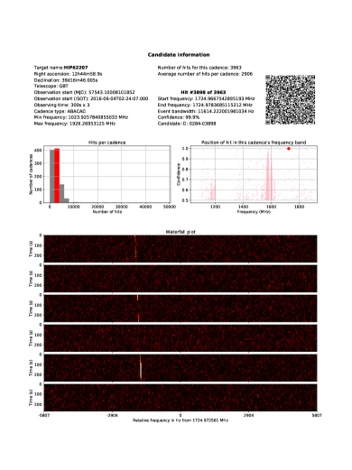
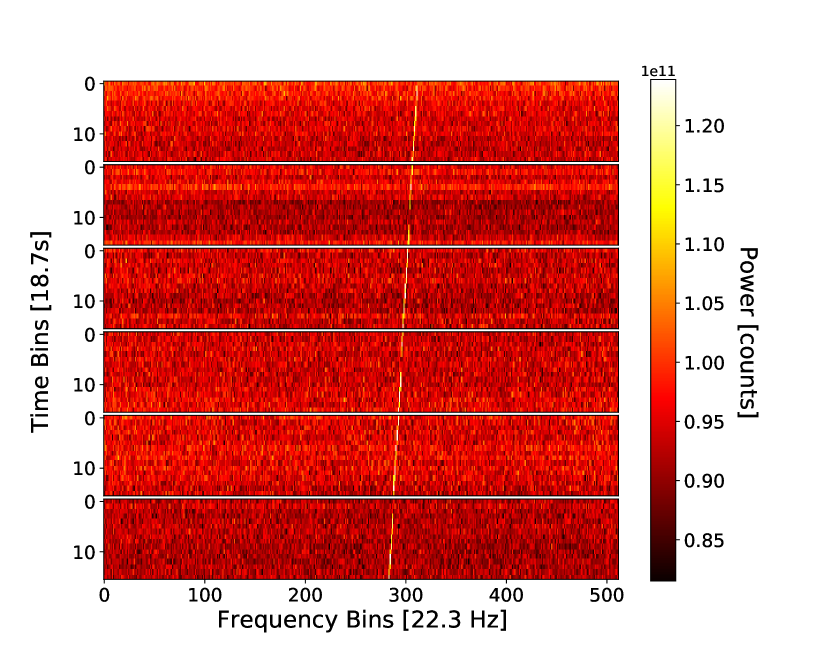
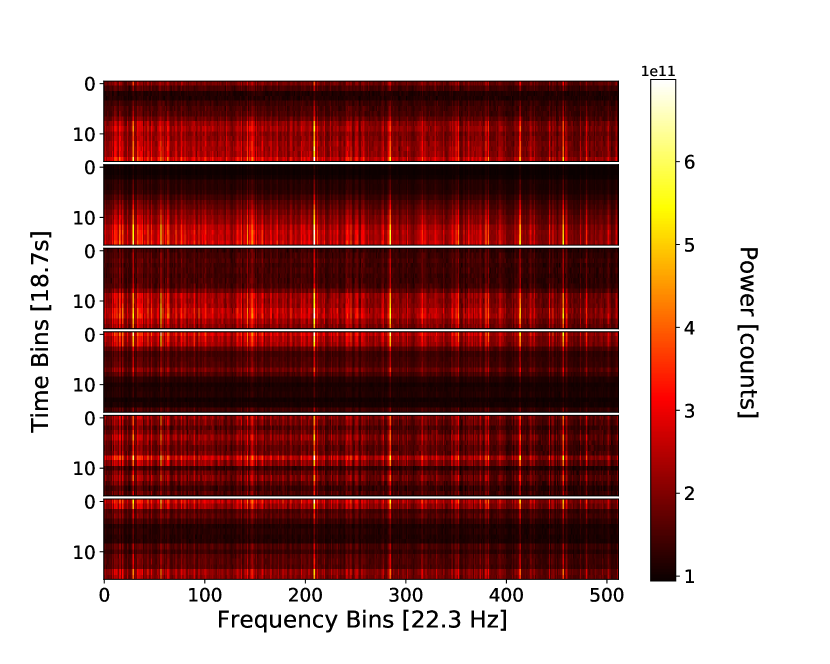
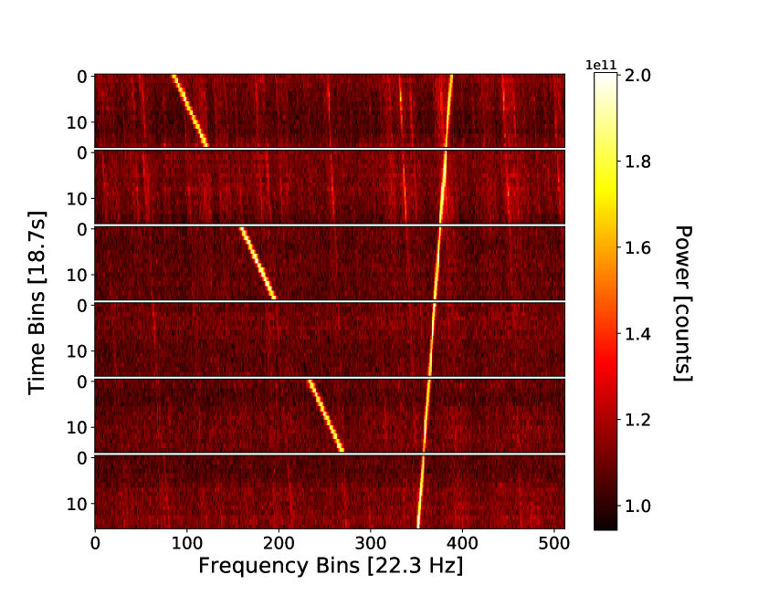
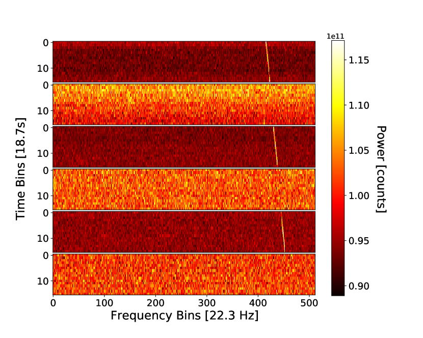
In order to display the information for each signal of interest snippet and to visually assess them, we create diagnostic plots for each of the 20,515 events returned by the ML model using a Python script. Supplementary Fig. 12 shows two examples of these diagrams, one for an event measured in the observation of HIP 54677 (described in Table 1 as MLc5, one of the top $8$ signals of interest of our search) and one for an event in HIP 114456, which is ultimately rejected upon human assessment due to the non-uniform drift rate across the three ON observations.

The header contains information about both the whole cadence and the signal of interest snippet from that cadence returned by the ML model. The information on the cadence includes the catalog name of its target star (the ON observation), its celestial coordinates (right ascension and declination), the telescope used, the start time of the observation written in both modified Julian day (MJD) and in ISO 8601 format for date and time (ISOT), the time spent observing ON-target, the cadence type (ABABAB or ABACAD), as well as the minimum and maximum frequency of this cadence recorded during the observation. Adding to this information are the number of events identified by the ML model for this specific cadence and the average number of events identified for all cadences. The information presented on the signal of interest includes the start and end frequencies of the snippet, the bandwidth of the snippet as well as the confidence rating according to the ML model. Each signal of interest is given a numerical identification composed of a number representing the cadence and a number representing the event snippet in that cadence. The header is juxtaposed with a QR code which encodes the ID of the signal of interest, the cadence target name, the start and end frequencies of the snippet as well as paths to the visualizer itself and to each of the six HDF5 files that make up the cadence. Paths correspond to locations on the Breakthrough Listen computers.

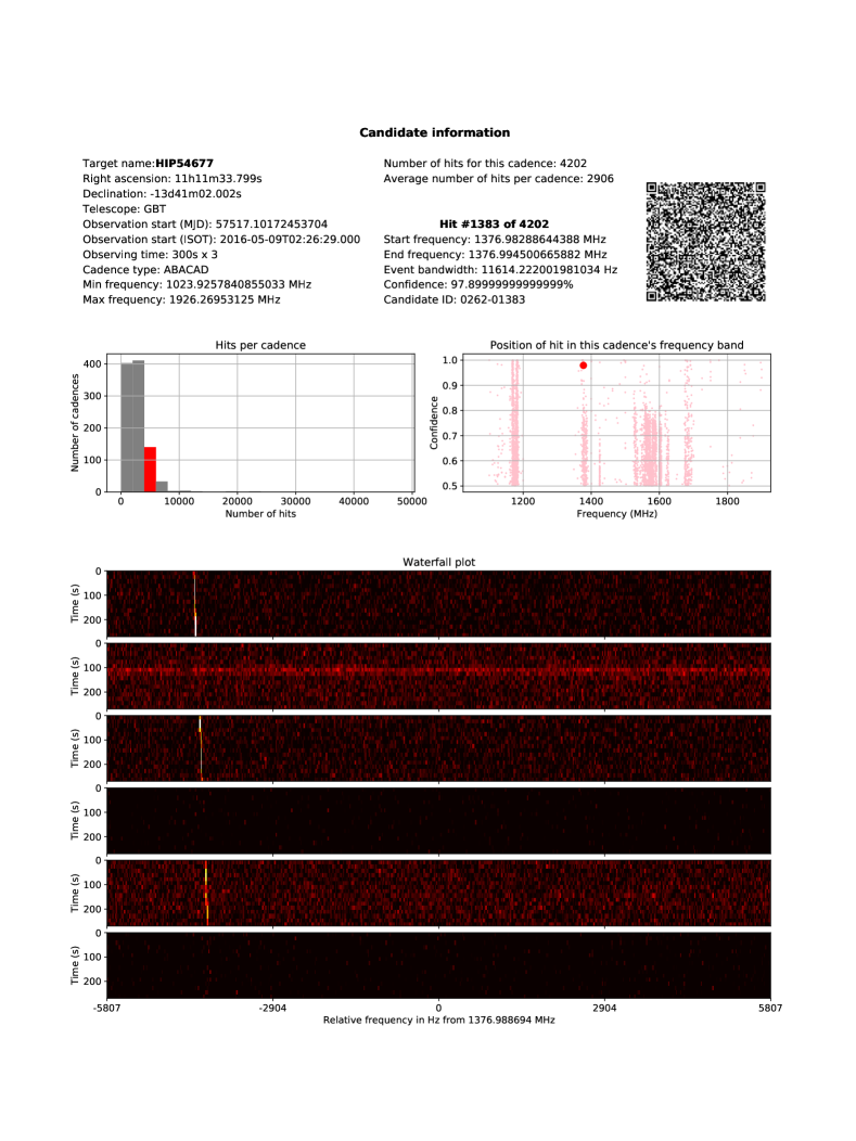
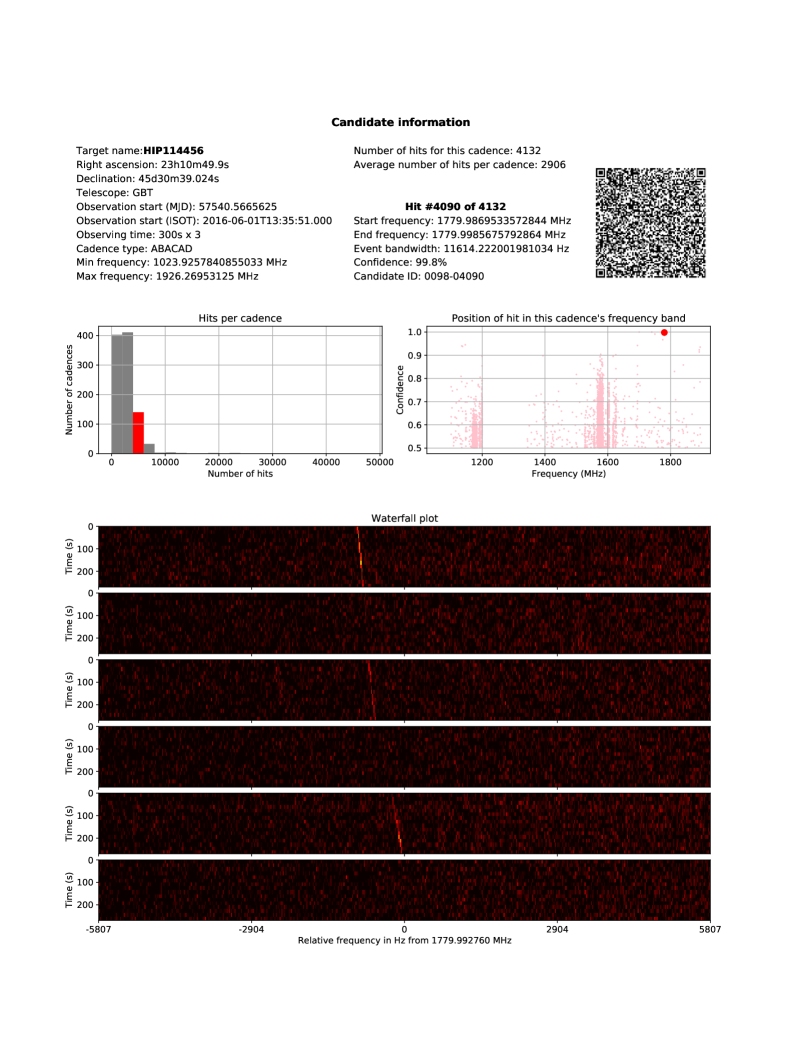
Two analytical plots are included in the middle of the diagram. The plot on the left is a histogram which classifies the cadences by the number of events identified in them, with the bin of the cadence in question highlighted in red. This is used to give a sense whether the specific cadence contains an unusually high amount of events (signals of interest) or not, as that might indicate an observation that is heavily contaminated by RFI and thus potentially less reliable. The plot on the right shows the positions of all events of a cadence in frequency space (i.e. where they fall in the bandwidth of the cadence) as well as the confidence ratings of the signals of interest. The signal of interest in question is represented by a large red dot in this plot. This plot helps to assess whether the specific signal of interest comes from a region of the frequency band that has a large number of events (higher chance that the signal of interest is also RFI) or if the region is relatively empty of events (higher chance that the signal of interest is genuinely special). Finally, the bottom half of the diagram is dedicated to the waterfall plot, a representation of frequency vs. time showing the signal of interest snippet across each of the six ON and OFF observations with lighter color signifying higher intensity. The waterfall plot is created using a modified version of the Python package blimpy¹¹¹¹11https://github.com/UCBerkeleySETI/blimpy and is downsampled by a factor of 8 in frequency, the same as the input dimension to the ML model. In other words, each frequency bin in the plot has a resolution about $\sim 22.4$ Hz.

All 20,515 diagrams generated are collated into an mp4 file to be viewed as a movie with four frames per second. The full video can be found at this weblink¹²¹²12https://www.youtube.com/watch?v=iSdVfOwPVCI.

Comparison with TurboSETI

One of the most extensively used SETI algorithms in Breakthrough Listen’s analysis is turboSETI¹³¹³13https://github.com/UCBerkeleySETI/turbo_seti as described in [3, 7], which is designed to detect these narrowband drifting signals by implementing the “tree de-Doppler” algorithm for incoherent Doppler acceleration searches[29]. One of the reasons we have chosen to work with this GBT dataset is because a thorough ETI search has previously been conducted on it using a standard de-Doppler technique [3, 5]. This provides a way to benchmark our algorithms as we can compare the output of two completely different methods. Out of the $1004$ cadences analyzed here, 688 were studied by [3] and 755 were in the sample used by [5]. The small mismatch in the source list is because we have rejected several cadences that have incomplete observations with less than 16 time bins, which are incompatible with our ML algorithm.

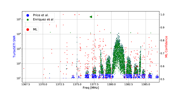
Supplementary Fig. 13 shows a comparison of the hits (not yet grouped per cadence to be considered as events) reported by these two turboSETI searches versus the events found by our ML algorithm on target HIP 54677 in the frequency ranges where we have detected our ETI signal of interest MLc5. The region around the signal of interest is clearly empty of any other detections. The blue and green TurboSETI hits essentially outline the GPS signal in the observing band. In fact eight out of the 11 prime signals-of-interest presented in [3] are from that particular region of 1370 $-$ 1380 MHz. Overall, we find that for every cadence, on average 64% of the events (with a deviation of 15%) flagged by our ML were not found by [3] and on average 61% (with a deviation of 37%) were not found by [5]. It thus appears that the events identified by the two search algorithms are quite distinct from each other.

Comparing our method to the conventional turboSETI, we find that our ML mode is successful in returning fewer false positives and more convincing signals of interest. Part of this is due to the fact that our ML model is built to consider the cadence pattern as a whole, whereas turboSETI searches each observation separately to produce hits, which then require a secondary grouping stage to cluster hits that come from the same signal of interest. We also note that our search has been able to cover a wider drift rate range up to $\pm$ 10 Hz/s and none of our top $8$ signals of interest were identified by the turboSETI searches [3, 5]. Our ML algorithm also has some disadvantages compared to turboSETI. One of them is that unlike turboSETI, we do not directly obtain drift rate and S/N as output of the pipeline. We also do not know precisely where the signal of interest lies in terms of observing frequency and only know within which 4096-channel snippet ( $\sim$ 11.6 kHz width) it is.

Code Availability

The code is available for review here at (https://github.com/PetchMa/ML_GBT_SETI)

Data Availability

All data used in this manuscript are stored as high-resolution filterbank and HDF5 format collected and generated from observations by the Robert C. Byrd Green Bank Telescope, which are available through the Breakthrough Listen Open Data Archive at http://seti.berkeley.edu/opendata. Correspondence and requests for other materials should be addressed to P.M.

Acknowledgements

Breakthrough Listen is managed by the Breakthrough Initiatives, sponsored by the Breakthrough Prize Foundation. (http://www.breakthroughinitiatives.org) We are grateful to the staff of the Green Bank Observatory for their help with installation and commissioning of the Breakthrough Listen backend instrument and extensive support during Breakthrough Listen observations. P.M. was supported by the Laidlaw foundation which has funded this project as part of the undergraduate research and leadership funding initiative. S.Z.S. acknowledges that this material is based upon work supported by the National Science Foundation MPS-Ascend Postdoctoral Research Fellowship under Grant No. 2138147. We thank Yuhong Chen for his helpful discussion on the Machine Learning framework. P.M. would like to thank the kind support of Dr. Laurance Doyle and Dr. Sarah Marzen for their generous guidance and encouragement to him when he first began his research career.