GPU Accelerated Newton for Taylor Series Solutions
of Polynomial Homotopies in Multiple Double Precision

Abstract

A polynomial homotopy is a family of polynomial systems, typically in one parameter $t$. Our problem is to compute power series expansions of the coordinates of the solutions in the parameter $t$, accurately, using multiple double arithmetic. One application of this problem is the location of the nearest singular solution in a polynomial homotopy, via the theorem of Fabry. Power series serve as input to construct Padé approximations.

Exploiting the massive parallelism of Graphics Processing Units capable of performing several trillions floating-point operations per second, the objective is to compensate for the cost overhead caused by arithmetic with power series in multiple double precision. The application of Newton’s method for this problem requires the evaluation and differentiation of polynomials, followed by solving a blocked lower triangular linear system. Experimental results are obtained on NVIDIA GPUs, in particular the RTX 2080, P100 and V100.

Code generated by the CAMPARY software is used to obtain results in double double, quad double, and octo double precision. The programs in this study are self contained, available in a public github repository under the GPL-v3.0 License.

Keywords and phrases. Graphics Processing Unit (GPU), multiple double arithmetic, Newton’s method, numerical analytic continuation, Taylor series.

1 Introduction

Many problems in science and engineering require the solving of a system of polynomial equations in several variables. Homotopy methods define families of polynomial systems which connect a system that must be solved to a system with known solutions. Continuation methods track the solution paths from the known solutions to solutions of the system that must be solved. This paper considers the application of Newton’s method to one solution path.

With multiple double arithmetic Taylor series developments for the solution curves defined by polynomial homotopies can be computed accurately using Newton’s method. The need for multiprecision in analytic continuation can be traced back to [13] via the direct quote “Some reflection shows that in order to get a convergent process the early vectors $A_{n}^{(k)}$ (early with respect to $k$) must be computed more accurately than the late ones” where the italics appear as in [13]. The early vectors refer to the earlier coefficients of the series. This quote appeared in abbreviated form in the recent paper [33].

The Taylor series coefficients are input to algorithms to construct Padé approximants [5], which are related to extrapolation methods [27] and approximation algorithms [32]. An example of an application to electrical engineering is the holomorphic embedding load flow method to solve power flow problems. In the convergence study of [8], results are computed with 400 digits of precision, using [22].

In this paper, acceleration with Graphics Processing Units (GPUs) is applied to compensate for the computational overhead caused by the multiple double arithmetic.

1.1 Problem Statement

The two main concerns are performance and convergence. For performance, the input must be sufficiently large, but still well conditioned enough to allow for Newton’s method to converge. The first problem is to define a setup that allows to scale so good performance can be reached while ensuring convergence. In examining the scalability we address the first key question: how much of the overhead can be compensated by GPU acceleration? Prior work showed that teraflop performance was achieved in the acceleration of the convolutions to evaluate and differentiate polynomials in several variables at power series [37] and in the acceleration of the blocked Householder QR [38] to solve linear systems in the least squares sense in multiple double precision. The differentiation adapts the reverse mode of algorithmic differentiation [11] with power series arithmetic. The acceleration of the blocked Householder QR [6] is explained in [19], and also addressed in [4] and [39]. Additional related work on multicore and accelerated QR can be found in [3], [2], [21], [30], and [31]. The acceleration of the back substitution algorithm applies the formulas of [12], developed further using the ideas of [26].

The second question concerns the combination of various kernels in the linearization of the power series. Of the various different types of kernels that are launched, which types require the most amount of time?

1.2 Multiprecision Arithmetic

A multiple double number is an unevaluated sum of nonoverlapping doubles. The renormalization and arithmetical operations are explained in [25].

MPLAPACK [24] supports quad double arithmetic and provides implementations of arbitrary multiprecision linear algebra operations. A recent application to matrix-matrix multiplication is in [34]. For multiple double precision, the software libraries QDlib [14] and CAMPARY [17] are applied, customized as follows. Instead of working with an array of double double numbers, two arrays of doubles are used: the first array for the most significant doubles and the second one for the least significant doubles, as this memory layout benefits memory coalescing, especially for complex quad double and octo double numbers. The GPU version of the QDlib library [23] uses the double2 and double4 types of the CUDA SDK, which promote good memory access for double doubles and quad doubles, but are not longer suited for complex quad doubles or octo doubles.

Multiple double precision is not true multiprecision in the sense that one cannot select any number of bits for the fraction. The other drawback is the limited size of the exponents (limited to the 11 bits of the 64-bit hardware doubles), which will prohibit the computation with infinitesimal values. In the context of GPU acceleration, recent work of [16] makes an interesting comparison with double double arithmetic: “The double double arithmetic of CAMPARY performs best for the problem of matrix-vector multiplication.” Concerning quad double precision, the authors of [16] write: “the CAMPARY library is faster than our implementation; however as the precision increases the execution time of CAMPARY also increases significantly.” The advantage of multiple double arithmetic is that simple counts of the number of floating-point operations quantify the cost overhead precisely and the flops metrics for performance are directly applicable.

The goal of applying GPU acceleration to offset the cost of multiple double precision arithmetic is related to the recent trend of mixed precision [1], [15], [18].

1.3 Numerical Condition of Taylor Series

The convergence concern is closely related to the numerical conditioning of the problem of power series solutions. Consider the following classical result, applied in [28] to detect nearby singularities.

Theorem 1.1 (the ratio theorem of Fabry [9])

If for the series $x(t)=c_{0}+c_{1}t+c_{2}t^{2}+\cdots+c_{d}t^{d}+c_{d+1}t^{d+1}+\cdots$, we have $\displaystyle\lim_{n\rightarrow\infty}c_{d}/c_{d+1}=z$, then

• $z$ is a singular point of the series, and

• it lies on the boundary of the circle of convergence of the series.

Then the radius of the circle of convergence is less than $|z|$.

In a numerical interpretation of this theorem, observe that the smaller convergence radius, the larger the growth in the coefficients, because then $|c_{d+1}|>|c_{d}|$. For example if $|z|$ is 1/2, then for sufficiently large $d$, $|c_{d+1}|\approx 2|c_{d}|$. Thus, for series of order 64, we could observe coefficients of magnitude $2^{64}\approx 1.8\times 10^{19}$. Therefore, for convergence, it is best to generate examples which have a unique power series solution and use decaying coefficients as in the series developments of exponential functions.

In this paper Newton’s method is applied to compute Taylor series. An alternative is to apply Fourier series methods as done in analytic continuation, see e.g. [10]. These methods are very sensitive to a good choice of the step size for taking samples of the function to be differentiated. As explained in [10] a smaller step size benefits the lower order coefficients while a larger step size may be needed to compute the higher order coefficients accurately.

This paper is another next step to accelerate a new robust path tracking algorithm [28], applying the linearization of [7] and extending the multicore implementation of [29]. As the robust path tracker of [28] scales well to track millions of paths without error, the context of this research effort is to scale the number of equations and variables of the systems. All code used in the experiments is publicly available in the github repository of PHCpack [35], released under the GNU GPL license.

The main experimental result of this research is that on systems of 1024 equations in 1024 variables, when doubling the precision from quad double to octo double, the increase in wall clock time is much less than what can be predicted from the cost overhead factors of the multiple double arithmetical operations as the increase in the time occupied by the kernels is significant. As expected, with multiple double arithmetic, the arithmetic intensity of the computations increases and the GPU becomes more fully occupied, allowing for a compensation of the cost overhead caused by the multiple double arithmetic.

The next section contains a high level description of Newton’s method on power series, using linearizations. The setup of the test problems with the levels of precision is justified in the third section. As defined in the fourth section, Newton’s method is executed using a staggered progression of the order of the power series. To predict the performance of the accelerated code, in section five the arithmetic intensities of different kernels are computed. Section six contains the results of the computational experiments.

2 Linearized Series and Newton’s Method

Figure 1: A task graph to solve a block Toeplitz system of four blocks as in (4). The arrows define data and execution flow. The length of the critical path determines the maximum speedup on a computer with 3 or more cores. With the fine granularity of instruction level parallelism of GPUs much larger speedups are obtained once the GPU is fully occupied. The computationally intensive qr is applied only once.

Instead of working with vectors and matrices of power series, we work with series that have as coefficients vectors and matrices. For example, for series of order 4, we solve $A(t){\bf x}(t)={\bf b}(t)$, with $n$-by-$n$ matrices $A_{0}$, $A_{1}$, $A_{2}$, $A_{3}$:

$$A(t) = A_{0}+A_{1}t+A_{2}t^{2}+A_{3}t^{3},$$ (1)

$${\bf x}(t) = {\bf x}_{0}+{\bf x}_{1}t+{\bf x}_{2}t^{2}+{\bf x}_{3}t^{3},$$ (2)

$${\bf b}(t) = {\bf b}_{0}+{\bf b}_{1}t+{\bf b}_{2}t^{2}+{\bf b}_{3}t^{3}.$$ (3)

The linearization of $A(t){\bf x}(t)={\bf b}(t)$ leads to

$$\left[\begin{array}[]{cccc}A_{0}&&&\\ A_{1}&A_{0}&&\\ A_{2}&A_{1}&A_{0}&\\ A_{3}&A_{2}&A_{1}&A_{0}\\ \end{array}\right]\left[\begin{array}[]{c}{\bf x}_{0}\\ {\bf x}_{1}\\ {\bf x}_{2}\\ {\bf x}_{3}\end{array}\right]=\left[\begin{array}[]{c}{\bf b}_{0}\\ {\bf b}_{1}\\ {\bf b}_{2}\\ {\bf b}_{3}\end{array}\right].$$ (4)

The task graph in Figure 1 defines a coarse grained parallel algorithm for $A(t){\bf x}(t)={\bf b}(t)$.

Even as least squares solutions provide an accuracy close to machine precision, in the forward substitution of the solution of the lower triangular block Toeplitz system in (4) the errors in the coefficient vectors ${\bf x}_{k}$ of ${\bf x}(t)$ propagate through the updates of the right hand side vectors ${\bf b}_{k}$, see Figure 1 for the update formulas. If we lose two decimal places of accuracy in each step, then for series of order four up to eight decimal places may be lost in the last coefficient vector ${\bf x}_{3}$. A more extensive error analysis was made in [29].

Newton’s method takes on input a system of polynomials in several variables, with power series truncated to the same degree and produces a sequence of power series. As an operator, this version of Newton’s method can be considered as turning a problem in many variables where all variables are interdependent into a sequence of power series for each separate variable, thus removing the interdependencies among the variables. A high level description of Newton’s method is shown in the pseudo code below.

	Input:	${\bf f}({\bf x}(t))$, system with power series coefficients;
		${\bf x}_{0}={\bf x}(t)$, initial leading coefficients;
		$N$, the maximum number of iterations;
		$\epsilon$, the tolerance on the accuracy.
	Output: $i$, the number of iterations;
	Output: ${\bf x}(t)$, if $i\leq N$, then $\|{\bf f}({\bf x}(t))\|<\epsilon$.
	${\bf x}(0):={\bf x}_{0}$
	for	$i$ from 1 to $N$ do
		$\displaystyle A(t),{\bf x}(t):=\partial({\bf f}({\bf x}(t)))$
		exit when $\|{\bf b}(t)\|<\epsilon$
		$\Delta{\bf x}(t):=A(t)\backslash{\bf b}(t)$
		report $\|{\bf b}(t)-A(t)\Delta{\bf x}(t)\|$
		${\bf x}(t):={\bf x}(t)+\Delta{\bf x}(t)$
		${\bf b}(t):={\bf b}(t)-A(t){\bf x}(t)$ as in Figure 1
		exit when $\|\Delta{\bf x}(t)\|<\epsilon$

The two computationally intensive operations are the evaluation and differentiation $\partial$ and the linear system solving $\backslash$. The residual computation $\|{\bf b}(t)-A(t)\Delta{\bf x}(t)\|$ is for monitoring the convergence of the method and can be omitted.

The high level description does not incorporate the staggered nature of the updates. As will be explained in section 4 below not all coefficient vectors of the series are involved in all stages.

3 Columns of Monomials

We start by considering polynomial systems of the form ${\bf x}^{E}={\bf b}(t)$, where $E$ is an exponent matrix which contains in its rows the exponent vectors of the variables ${\bf x}$. The right hand side ${\bf b}(t)$ is a vector of power series. For example, $n=3$, ${\bf x}=[x_{1},x_{2},x_{3}]$:

$$E=\left[\begin{array}[]{ccc}1&0&0\\ 1&1&0\\ 1&1&1\end{array}\right]\quad\left\{\begin{array}[]{lcl}x_{1}&\!\!\!=\!\!\!&b_{1}(t)\\ x_{1}x_{2}&\!\!\!=\!\!\!&b_{2}(t)\\ x_{1}x_{2}x_{3}&\!\!\!=\!\!\!&b_{3}(t)\end{array}\right.$$ (5)

with solutions

$$\begin{array}[]{l}x_{1}(t)=\exp(\alpha_{1}t)+O(t^{d})\\ x_{2}(t)=\exp(\alpha_{2}t)+O(t^{d})\\ x_{3}(t)=\exp(\alpha_{3}t)+O(t^{d})\end{array}$$ (6)

where

$$\exp(\alpha t)+O(t^{4})=1+\alpha t+\frac{\alpha^{2}}{2!}t^{2}+\frac{\alpha^{3}}{3!}t^{3}+O(t^{4}),$$ (7)

with $\alpha\in[-1,-1+\delta]\cup[1-\delta,1]$, $\delta>0$, or $|\alpha|=1$ for random $\alpha\in{\mathbb{C}}$. The $\alpha$ introduces numerical variation in the coefficients of the solutions.

The choice of exponential series as solution series avoids that the series in the right hand side vector of the system become large. Considering the series expansion

$$\exp(t)=\sum_{k=0}^{d-1}\frac{t^{k}}{k!}+O(t^{d})$$ (8)

leads in Table 1 to a justification for multiprecision, based on the size of the last coefficient in the truncated series. The levels of precision proceeds in powers of two according to the expected quadratic convergence of Newton’s method.

$k$	$1/k!$	recommended precision	eps
7	2.0e-004	double precision okay	2.2e-16
15	7.7e-013	use double doubles	4.9e-32
23	3.9e-023	use double doubles
31	1.2e-034	use quad doubles	6.1e-64
47	3.9e-060	use octo doubles	4.6e-128
63	5.0e-088	use octo doubles
95	9.7e-149	need hexa doubles	5.3d-256
127	3.3e-214	need hexa doubles

Table 1: Recommended precision levels based on the order of the series, where eps is the smallest positive double that makes a difference when added to 1.0.

The need hexa doubles in Table 1 is because accelerating the least squares solving, evaluation and differentiation at power series with hexa double arithmetic is still a work in progress. The computations in this paper are therefore limited to series of order 64. While computations of larger orders are possible, the accuracy in octo double precision is no longer guaranteed.

While one column of monomials is sufficient for convergence and scalability investigations, consider the 2-column format of monomials

$${\bf c}_{1}{\bf x}^{E_{1}}+{\bf c}_{2}{\bf x}^{E_{2}}={\bf b}(t),$$ (9)

for two $n$-vectors ${\bf c}_{1}$ and ${\bf c}_{2}$ and two exponent matrices $E_{1}$ and $E_{2}$. With the introduction of new variables, any polynomial system can be written in this 2-column format.

For the experiments with two columns of monomials, specific lower and upper triangular matrices of ones are used. For example, for $n=3$:

$$E_{1}=\left[\begin{array}[]{ccc}1&0&0\\ 1&1&0\\ 1&1&1\end{array}\right]\quad\mbox{and}\quad E_{2}=\left[\begin{array}[]{ccc}1&1&1\\ 1&1&0\\ 1&0&0\end{array}\right].$$ (10)

Although the product of the degrees of the system ${\bf c}_{1}{\bf x}^{E_{1}}+{\bf c}_{2}{\bf x}^{E_{2}}={\bf b}(t)$ is now much larger than the systems defined by ${\bf x}^{E_{1}}={\bf b}(t)$ and ${\bf x}^{E_{2}}={\bf b}(t)$, there is still only one solution, which allows for decaying coefficients in the power series and thus for coefficients of modest growth, benefiting the numerical conditioning of the problem.

That ${\bf c}_{1}{\bf x}^{E_{1}}+{\bf c}_{2}{\bf x}^{E_{2}}={\bf b}(t)$, for lower and upper triangular matrices $E_{1}$ and $E_{2}$ as in (10), has only one solution can be seen by considering the $k$-th and the $(n-k)$-th equations:

$$k : c_{1,k\hphantom{-k}}{\bf x}^{{\bf e}_{1,k\hphantom{-k}}}+c_{2,k\hphantom{-k}}{\bf x}^{{\bf e}_{2,k\hphantom{-k}}}=b_{k}(t)$$

$$n-k : c_{1,n-k}{\bf x}^{{\bf e}_{1,n-k}}+c_{2,n-k}{\bf x}^{{\bf e}_{2,n-k}}=b_{n-k}(t).$$

As ${\bf e}_{1,k}={\bf e}_{2,n-k}$ and ${\bf e}_{2,k}={\bf e}_{1,n-k}$, the two equations can be diagonalized into

$$\gamma_{1,k}{\bf x}^{{\bf e}_{1,k}} = \beta_{k}(t)$$

$$\gamma_{1,n-k}{\bf x}^{{\bf e}_{1,n-k}} = \beta_{n-k}(t),$$

so for those two particular choices of $E_{1}$ and $E_{2}$ the system is equivalent to the one-column system ${\bf x}^{E}={\bf b}(t)$ which has a unique solution series.

While ${\bf c}_{1}{\bf x}^{E_{1}}+{\bf c}_{2}{\bf x}^{E_{2}}={\bf b}(t)$ has thus the same good numerical conditioning as ${\bf x}^{E}={\bf b}(t)$, it serves as a good test on the increased cost of evaluation and differentiation. For problems with many nearby singularities, it is recommended to work with a factor $\delta\in(0,1)$ to multiply the parameter $t$ with to dampen the growth of the coefficients in the series, according to the numerical interpretation of Theorem 1.1.

4 Staggered Computations

In computing ${\bf x}(t)={\bf x}_{0}+{\bf x}_{1}t+{\bf x}_{2}t^{2}+\cdots+{\bf x}_{d-1}t^{d-1}$, not all $d$ coefficient vectors need to be involved.

We start ${\bf x}_{0}$ with half its precision correct, otherwise Newton’s method may not converge. The first iteration consists in getting ${\bf x}_{0}$ correct to the full working precision. If Newton’s method would not converge for order zero, then there is no use of increasing the order.

The $d$ in the order $O(t^{d})$ is increased gradually, for example, the update formula for the order

$$d:=d+1+d/2$$ (11)

is optimistically hoping for quadratic convergence.

Once ${\bf x}_{k}$ is correct, the corresponding ${\bf b}_{k}=0$, as ${\bf b}_{k}$ is obtained by evaluation, and then the update $\Delta{\bf x}_{k}$ should no longer be computed because

$$QR\Delta{\bf x}_{k}={\bf b}_{k}={\bf 0}\quad\Rightarrow\quad\Delta{\bf x}_{k}={\bf 0}.$$ (12)

This gives a criterion to stop the iterations.

5 Accelerating Newton’s Method

While the blocked Householder QR is very suitable to GPU acceleration and teraflop performance is achieved already at relatively modest dimensions, it stars only at the very beginning of Newton’s method as it is no longer needed once the QR decomposition is computed. The second part of the least squares solver, the back substitution, is needed in every stage, as are the convolutions to compute the right hand sides of the linear systems.

In [20], the Compute to Global Memory Access (CGMA) ratio is defined as the number of floating-point calculations performed by a kernel for each access to the global memory. This CGMA ratio corresponds to the more general notion of arithmetic intensity of a computation [40].

5.1 Arithmetic Intensity of Convolutions

In the computation of the arithmetic intensity of convolutions, or equivalently, the number of floating-point computations per double, it suffices to consider one monomial. For example, take $n=4$ and let $f=x_{1}x_{2}x_{3}x_{4}$ be the monomial we evaluate and differentiate. Using the reverse mode of algorithmic differentiation, the computations are organized as follows:

$$\begin{array}[]{lll}x_{1}\star x_{2}&x_{4}\star x_{3}&x_{1}x_{2}\\ x_{1}x_{2}\star x_{3}&x_{4}x_{3}\star x_{2}&x_{4}x_{3}\star x_{1}\\ x_{x}x_{2}x_{3}\star x_{4}\end{array}$$ (13)

where each $\star$ indicates a new multiplication. In the three columns we count respectively $n-1=3$, $n-2=2$, $n-2=2$, for a total of $3n-5$ multiplications, for $n$ inputs. If the inputs were doubles, then the arithmetic intensity would be

$$\frac{3n-5}{n}.$$ (14)

Each input is a power series of order $d$. To avoid thread divergence, the coefficients of the second series in each product are padded with zeros. For example, for $d=3$:

$$\begin{array}[]{ll}&(a_{0}+a_{1}t+a_{2}t^{2})(b_{0}+b_{1}t+b_{2}t^{2})\\ =&(a_{0}\star b_{0}+a_{1}\star b_{-1}+a_{2}\star b_{-2})\\ +&(a_{0}\star b_{1}+a_{1}\star b_{0\phantom{-}}+a_{2}\star b_{-1})t\\ +&(a_{0}\star b_{2}+a_{1}\star b_{1\phantom{-}}+a_{2}\star b_{0}\phantom{-})t^{2},\end{array}$$ (15)

where coefficients with negative indices are zero. Ignoring the additions, we count $d^{2}$ multiplications, so we now have $(3n-5)d^{2}$ multiplications for $nd$ inputs. If the coefficients of the power series were doubles, then the arithmetic intensity would be

$$\frac{(3n-5)d^{2}}{nd}.$$ (16)

The coefficients of the power series are multiple doubles. For double double, quad double, and octo double, the number of doubles in the inputs are respectively $2nd$, $4nd$, and $8nd$. Working with complex coefficients doubles the size of the input. Doubling the precision doubles the size of the input, but increase the arithmetical cost significantly, as illustrated by Table 2 (with data from [36]).

	$+$	$-$	$*$	total
double double	5	9	9	23
quad double	99	164	73	336
octo double	529	954	259	1742

Table 2: Arithmetical Cost of Multiple Double Multiplications, e.g.: multiplying two double doubles takes 5 additions of two doubles, 9 subtractions and 9 multiplications, for a total of 23 floating-point operations.

Then the number of floating-point operations per double for the evaluation and differentiation of a product of $n$ power series of order $d$ are respectively for double doubles, quad doubles, and octo doubles:

$$\frac{23(3n-5)d^{2}}{2nd},~{}~{}\frac{336(3n-5)d^{2}}{4nd},~{}~{}\frac{1742(3n-5)d^{2}}{8nd},$$ (17)

where the corresponding multiplication factors $23/2$, $336/4$, and $1742/8$ evaluate respectively to 11.5, 84, and 217.75.

With each doubling of the precision, the arithmetic intensity increases by a factor of 11.5 (from double to double double), by a factor of $7.30\approx 84/11.5$ (from double double to quad double), and by a factor of $2.59\approx 217.75/84$ (from quad double to octo double). As the evaluation and differentiation is needed at every stage of Newton’s method, the high numbers of floating-point operations per double are promising indicators for the success of GPU acceleration.

5.2 Accelerated Least Squares

With the QR decomposition of a matrix $A$, solving $A{\bf x}={\bf b}$ in the least squares sense is reduced to $R{\bf x}=Q^{H}{\bf b}$, which involves the multiplication of $Q^{H}$ with ${\bf b}$, followed by a back substitution.

Assuming the leading coefficient vector ${\bf x}_{0}$ of the series has an accuracy of at least half the working precision, the QR decomposition happens only once in the first stage of Newton’s method, at a cost of $O(n^{3})$. While every stage involves the solution of $R{\bf x}=Q^{H}{\bf b}$, the cost of computing $Q^{H}{\bf b}$ and the back substitution is both $O(n^{2})$. Even if the acceleration of the QR decomposition works better than the acceleration of $R{\bf x}=Q^{H}{\bf b}$, the factor $n$ in the cost overhead of QR over $R{\bf x}=Q^{H}{\bf b}$ makes that the proportion of the QR decomposition will still dominate all $Q^{H}{\bf b}$ computations and all back substitutions, as $n$ equals 1024 and the number of stages is capped to 24.

5.3 Accelerated Updates and Residuals

The updates of the right hand side vectors (see the right of Figure 1) involve many different matrices. For example, the updates to ${\bf b}_{3}$ happen as ${\bf b}_{3}:={\bf b}_{3}-A_{3}{\bf x}_{0}$, ${\bf b}_{3}:={\bf b}_{3}-A_{2}{\bf x}_{1}$, ${\bf b}_{3}:={\bf b}_{3}-A_{1}{\bf x}_{2}$, each time with different matrices $A_{3}$, $A_{2}$, and $A_{1}$ which cannot remain all in the main memory of the device. Even as the cost of these computations is $O(n^{2})$ we may expect the updates to occupy a significant portion of the total execution times.

The same arguments apply to the computation of the residuals, when measuring the accuracy of the computed updates $\Delta{\bf x}$. However, one could significantly reduce the cost by selecting only one or a few random equations instead of computing the residuals for all equations.

For comparison with the arithmetic intensities of the convolutions, consider the matrix-vector product, for an $n$-by-$n$ matrix. Executed on doubles, $n^{2}$ multiplications are performed on $(n+1)n$ doubles. The ratio $n^{2}/(n^{2}+n)$ improves on power series of order $d$, as convolutions with padding take $d^{2}$ multiplications, while the size of the data is multiplied by $d$. Restricting to multiplications, the arithmetic intensity then is

$$\frac{n^{2}d^{2}}{(n+1)nd}\approx d.$$ (18)

Compared to the arithmetic intensity of convolutions, the leading terms of the numerator of (16) divided by the denominator evaluates to $3d$. So the arithmetic intensity of convolutions is three times more than that of matrix-vector products.

NVIDIA GPU	CUDA	#MP	#cores/MP	#cores	GHz
Pascal P100	6.0	56	64	3584	1.33
Volta V100	7.0	80	64	5120	1.91
GeForce RTX 2080	7.5	46	64	2944	1.10
NVIDIA GPU	host CPU			RAM	GHz
Pascal P100	Intel E5-2699			256 GB	2.20
Volta V100	Intel W2123			32 GB	3.60
GeForce RTX 2080	Intel i9-9880H			32 GB	2.30

Table 3: Specifications of the GPUs.

6 Computational Results

The computational experiments attempt to answer the following three questions. Classifying the types of kernels into three categories: convolutions, least squares, updates and residuals, which type of kernel occupies the largest portion of the overall execution time? For which order of the series do we reach teraflop performance? What happens to the wall clock time when the precision is doubled?

6.1 Graphics Processing Units

The code was developed for the “Volta” V100 NVIDIA GPU, and tested on the “Pascal” P100 and RTX 2080 NVIDIA GPUs. Table 3 lists the main characteristics of the GPUs.

The double precision peak performance of the P100 is 4.7 TFLOPS. At 7.9 TFLOPS, the V100 is 1.68 times faster than the P100. To evaluate the algorithms, compare the ratios of the wall clock times on the P100 over V100 with the factor 1.68. For every kernel, the number of arithmetical operations is accumulated. The total number of double precision operations is computed using the cost overhead multipliers.

6.2 Proportions of Kernel Times

We distinguish six different types of kernels: (1) convolutions for evaluation and differentiation; (2) Householder QR; (3) $Q^{H}{\bf b}$ computations; (4) back substitutions to solve $R{\bf x}=Q^{H}{\bf b}$; (5) updates ${\bf b}:={\bf b}-A{\bf x}$; and (6) residual computations $\|{\bf b}-A{\bf x}\|_{1}$. Visualizing the data in Table 4, Figure 2 shows the percentages of the kernels on one column of monomials defined by a triangular exponent matrix of dimension 1024 to compute series of order 64 in octo double precision, done on the V100.

kernel	one column	two columns
convolution	121.386	244.535
Householder QR	24.451	24.123
kernel for $Q^{T}{\bf b}$	5.849	6.139
back substitution	17.053	17.884
updates	111.474	124.080
residuals	125.122	137.963
total time	405.334	554.723
wall clock time	1129.794	1808.480

Table 4: Times in seconds for each kernel on V100, on one column and two columns of monomials in octo double precision.

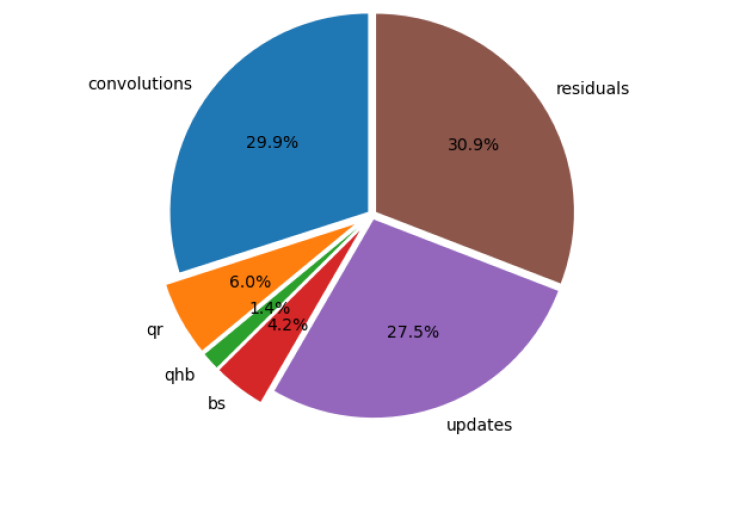
Figure 2: Percentage of each type of accelerated computation for a one column monomial system in octo double precision, on V100.

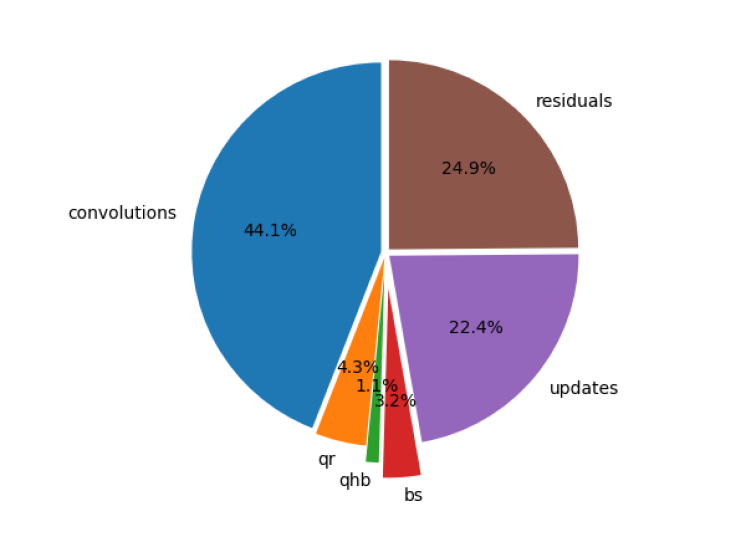
Figure 3: Percentage of each type of accelerated computation for a two column monomial system in octo double precision, on V100.

The largest portion of the time goes to the residual computations, for all equations in the system. The residuals are important to measure the convergence and must be computed in multiple double precision. One optimization could be to select at random one or a couple of equations and compute the residuals for those selected equations instead of for all equations. Figure 3 shows that for a 2-column monomial system, the time spent on convolutions dominates.

order	P100	V100
1	8.041	28.997
2	16.191	59.820
3	23.748	90.003
5	29.277	149.894
8	62.747	240.760
12	94.035	360.816
18	140.918	540.572
27	211.261	810.645
41	351.994	1045.032
62	535.136	1569.347
64	554.654	1658.382

Table 5: Performance in gigaflops of convolution on P100 and V100 to evaluate and differentiate one column of 1024 monomials in octo double precision.

6.3 Performance of Convolutions

Figure 2 shows that the convolutions occupy a substantial part of the computations. For what orders of the series do we observe teraflop performance? Consider Table 5.

On one column of monomials, triangular exponent matrix of ones, $n=1024$, performance of the evaluation and differentiation, in octo double precision, for increasing orders of the series, visualizing the data in Table 5, Figure 4 shows that teraflop performance is observed after order 40 on the V100. But on the P100 only half a teraflop is reached at order 64.

Figure 4: Performance in gigaflops on the P100 (top) and on the V100 (bottom) to evaluate and differentiation at series in octo double precision versus the order of the series.

In the current implementation, in the convolution of two power series each thread is responsible for one coefficient of the result. Threads are launched in blocks of the size that match the number of coefficients. An implementation better suited for series of lower order would employ a finer granularity and have several threads collaborate to compute one coefficient of a convolution of two series.

6.4 Doubling the Precisions

To investigate how much of the cost overhead can be compensated by the acceleration consider the wall clock times and the elapsed times spend by all kernels when the precision is doubled.

	D	2D	4D	8D
P100 kernel times	10.4	44.5	204.4	1263.3
wall clock	418.5	695.3	969.9	3073.6
V100 kernel times	6.2	22.6	146.4	405.3
wall clock	277.9	475.3	834.7	1129.8

Table 6: Wall clock times in seconds for double (D), double double (2D), quad double (4D), and octo double (8D) for one column of 1024 monomials to compute series of order 64 on P100 and V100.

Visualizing Table 6, Figure 5 shows the 2-logarithms of the times of 24 steps with Newton’s method on one column of monomials defined by a triangular exponent matrix of ones of dimension 1024, on the V100. Doubling the precision less than doubles the wall clock time and increases the time spent by all kernels.

Figure 5: In doubling the precision, the wall clock times on P100 (top) and V100 (bottom) less than doubles as the proportion of the elapsed times spent by all kernels increases.

6.5 Experiments on the RTX 2080

	D	2D	4D	8D
Kernel times	1.4	16.6	122.4	380.1
wall clock	35.7	80.0	225.0	474.8

Table 7: Wall clock times in seconds for double (D), double double (2D), quad double (4D), and octo double (8D) for one column of 1024 monomials to compute series of order 64 on RTX 2080.

The last experiments concern the RTX 2080, on 16 steps with Newton’s method on one column of monomials defined by a triangular exponent matrix of ones of dimension 512. The results are summarized in Figure 6, visualizing the data in Table 7.

Figure 6: Doubling the precision on the RTX 2080.

Although several optimizations in the code will improve the performance, this first implementation offers a promising first step towards a scalable nonlinear solver based on results from numerical analytic continuation.

7 Conclusions

Using decaying coefficients of power series expansions, octo double precision suffices for series of order 64. Teraflop performance of the evaluation and differentiation is already attained at order 40 on the V100. The convolutions to evaluate and differentiate at power series remain a significant portion of all computational work. For two columns of monomials which can encode general polynomial systems, the computational effort to evaluate and differentiate dominates all other kernels.

Doubling precisions less than doubles the wall clock times because the computations are then compute bound and thus well suited for acceleration by graphics processing units. Extending the acceleration beyond octo double precision on GPUs more recent than the V100 is a future direction.

References

- [1] A. Abdelfattah, H. Anzt, E. G. Boman, E. Carson, T. Cojean, J. Dongarra, A. Fox, M. Gates, N. J. Higham, X. S. Li, J. Loe, P. Luszczek, S. Pranesh, S. Rajamanickam, T. Ribizel, B. F. Smith, K. Swirydowicz, S. Thomas, S. Tomov, Y. M. Tsai, and U. M. Yang. A survey of numerical linear algebra methods utilizing mixed-precision arithmetic. International Journal of High Performance Computing Applications, 35(4):344–369, 2021.
- [2] E. Agullo, C. Augonnet, J. Dongarra, and M. Faverge. QR factorization on a multicore node enhanced with multiple GPU accelerators. In 2011 IEEE International Parallel and Distributed Processing Symposium, pages 932–943. IEEE, 2011.
- [3] M. Anderson, G. Ballard, J. Demmel, and K. Kreutzer. Communication-avoiding QR decomposition for GPUs. In 2011 IEEE International Parallel and Distributed Processing Symposium, pages 48–58. IEEE, 2011.
- [4] M. Baboulin, J. Dongarra, and S. Tomov. Some issues in dense linear algebra for multicore and special purpose architectures. Technical Report UT-CS-08-200, University of Tennessee, 2008.
- [5] Baker, Jr, G. A. and P. Graves-Morris. Padé Approximants. Cambridge University Press, 1996.
- [6] C. Bischof and C. F. Van Loan. The WY representation for products of Householder matrices. SIAM J. Sci. Stat. Comput., 8(1):s1–s13, 1987.
- [7] N. Bliss and J. Verschelde. The method of Gauss-Newton to compute power series solutions of polynomial homotopies. Linear Algebra and its Applications, 542:569–588, 2018.
- [8] A. Dronamraju, S. Li, Q. Li, Y. Li, D. Tylavsky, D. Shi, and Z. Wang. Implications of Stahl’s theorems to holomorphic embedding part II: numerical convergence. CSEE Journal of Power and Energy Systems, 7(4):773–784, 2021.
- [9] E. Fabry. Sur les points singuliers d’une fonction donnée par son développement en série et l’impossibilité du prolongement analytique dans des cas très généraux. Annales scientifiques de l’École Normale Supérieure, 13:367–399, 1896.
- [10] B. Fornberg. Numerical differentiation of analytic functions. ACM Transactions on Mathematical Software, 7(4):512–526, 1981.
- [11] A. Griewank and A. Walther. Evaluating Derivatives: Principles and Techniques of Algorithmic Differentiation. SIAM, second edition, 2008.
- [12] D. H. Heller. A survey of parallel algorithms in numerical linear algebra. SIAM Review, 20(4):740–777, 1978.
- [13] P. Henrici. An algorithm for analytic continuation. SIAM Journal on Numerical Analysis, 3(1):67–78, 1966.
- [14] Y. Hida, X. S. Li, and D. H. Bailey. Algorithms for quad-double precision floating point arithmetic. In 15th IEEE Symposium on Computer Arithmetic (Arith-15 2001), pages 155–162. IEEE Computer Society, 2001.
- [15] N. J. Higham and T. Mary. Mixed precision algorithms in numerical linear algebra. Acta Numerica, pages 347–414, 2022.
- [16] K. Isupov and V. Knyazkov. Multiple-precision matrix-vector multiplication on graphics processing units. Program Systems: Theory and Applications, 11(3):62–84, 2020.
- [17] M. Joldes, J.-M. Muller, V. Popescu, and Tucker. W. CAMPARY: Cuda Multiple precision arithmetic library and applications. In Mathematical Software – ICMS 2016, the 5th International Conference on Mathematical Software, pages 232–240. Springer-Verlag, 2016.
- [18] C. T. Kelley. Newton’s method in mixed precision. SIAM Review, 64(1):191–211, 2022.
- [19] A. Kerr, D. Campbell, and M. Richards. QR decomposition on GPUs. In D. Kaeli and M. Leeser, editors, Proceedings of 2nd Workshop on General Purpose Processing on Graphics Processing Units (GPGPU’09), pages 71–78. ACM, 2009.
- [20] D. B. Kirk and W. W. Hwu. Programming Massively Parallel Processors. A Hands-on Approach. Morgan Kaufmann, 2010.
- [21] J. Kurzak, R. Nath, P. Du, and J. Dongarra. An implementation of the tile QR factorization for a GPU and multiple GPUs. In Applied Parallel and Scientific Computing, 10th International Conference, PARA 2010, volume 7134 of Lecture Notes in Computer Science, pages 248–257. Springer-Verlag, 2012.
- [22] Advanpix LLC. Multiprecision computing toolbox for MATLAB. www.advanpix.com.
- [23] M. Lu, B. He, and Q. Luo. Supporting extended precision on graphics processors. In Proceedings of the Sixth International Workshop on Data Management on New Hardware (DaMoN 2010), pages 19–26, 2010.
- [24] N. Maho. MPLAPACK version 2.0.1. user manual. arXiv:2109.13406v2 [cs.MS] 12 Sep 2022.
- [25] J.-M. Muller, N. Brunie, F. de Dinechin, C.-P. Jeannerod, M. Joldes, V. Lefèvre, G. Melquiond, N. Revol, and S. Torres. Handbook of Floating-Point Arithmetic. Springer-Verlag, second edition, 2018.
- [26] W. Nasri and Z. Mahjoub. Optimal parallelization of a recursive algorithm for triangular matrix inversion on MIMD computers. Parallel Computing, 27:1767–1782, 2001.
- [27] A. Sidi. Practical Extrapolation Methods. Theory and Applications, volume 10 of Cambridge Monographs on Applied and Computational Mathematics. Cambridge University Press, 2003.
- [28] S. Telen, M. Van Barel, and J. Verschelde. A robust numerical path tracking algorithm for polynomial homotopy continuation. SIAM Journal on Scientific Computing, 42(6):3610–A3637, 2020.
- [29] S. Telen, M. Van Barel, and J. Verschelde. Robust numerical tracking of one path of a polynomial homotopy on parallel shared memory computers. In Proceedings of the 22nd International Workshop on Computer Algebra in Scientific Computing (CASC 2020), volume 12291 of Lecture Notes in Computer Science, pages 563–582. Springer-Verlag, 2020.
- [30] S. Tomov, J. Dongarra, and M. Baboulin. Towards dense linear algebra for hybrid GPU accelerated manycore systems. Parallel Computing, 36(5):232–240, 2010.
- [31] S. Tomov, R. Nath, H. Ltaief, and J. Dongarra. Dense linear algebra solvers for multicore with GPU accelerators. In The 2010 IEEE International Parallel and Distributed Processing Symposium Workshops (IPDPSW), pages 1–8. IEEE, 2010.
- [32] L. N. Trefethen. Approximation Theory and Approximation Practice. SIAM, 2013.
- [33] L. N. Trefethen. Quantifying the ill-conditioning of analytic continuation. BIT Numerical Mathematics, 60(4):901–915, 2020.
- [34] T. Utsugiri and T. Kouya. Acceleration of multiple precision matrix multiplication using Ozaki scheme. arXiv:2301.09960v2 [math.NA] 25 Jan 2023.
- [35] J. Verschelde. Algorithm 795: PHCpack: A general-purpose solver for polynomial systems by homotopy continuation. ACM Trans. Math. Softw., 25(2):251–276, 1999.
- [36] J. Verschelde. Parallel software to offset the cost of higher precision. ACM SIGAda Ada Letters, 40(2):59–64, 2020.
- [37] J. Verschelde. Accelerated polynomial evaluation and differentiation at power series in multiple double precision. In The 2021 IEEE International Parallel and Distributed Processing Symposium Workshops (IPDPSW), pages 740–749. IEEE, 2021.
- [38] J. Verschelde. Least squares on GPUs in multiple double precision. In The 2022 IEEE International Parallel and Distributed Processing Symposium Workshops (IPDPSW), pages 828–837. IEEE, 2022.
- [39] V. Volkov and J. Demmel. Benchmarking GPUs to tune dense linear algebra. In Proceedings of the 2008 ACM/IEEE conference on Supercomputing. IEEE Press, 2008. Article No. 31.
- [40] S. Williams, A. Waterman, and D. Patterson. Roofline: an insightful visual performance model for multicore architectures. Communications of the ACM, 52(4):65–76, 2009.