Active Sequential Two-Sample Testing

Abstract

Two-sample testing tests whether the distributions generating two samples are identical. We pose the two-sample testing problem in a new scenario where the sample measurements (or sample features) are inexpensive to access, but their group memberships (or labels) are costly. We devise the first active sequential two-sample testing framework that not only sequentially but also actively queries sample labels to address the problem. Our test statistic is a likelihood ratio where one likelihood is found by maximization over all class priors, and the other is given by a classification model. The classification model is adaptively updated and then used to guide an active query scheme called bimodal query to label sample features in the regions with high dependency between the feature variables and the label variables. The theoretical contributions in the paper include proof that our framework produces an anytime-valid $p$-value; and, under reachable conditions and a mild assumption, the framework asymptotically generates a minimum normalized log-likelihood ratio statistic that a passive query scheme can only achieve when the feature variable and the label variable have the highest dependence. Lastly, we provide a query-switching (QS) algorithm to decide when to switch from passive query to active query and adapt bimodal query to increase the testing power of our test. Extensive experiments justify our theoretical contributions and the effectiveness of QS.

1 Introduction

A two-sample test is a statistical hypothesis test which is applied on data samples (or measurements) from two distributions. The goal is to test if the data support the hypothesis that the distributions are different. If one were to think of each data point as being composed of features and group membership labels (which tell us which distribution the data is from), then the two-sample test is equivalent to the problem of testing the dependence between the features and the labels. With these lens, the null hypothesis for the two-sample test claims the independence of feature variables and the label variables; the alternate hypothesis states the opposite. A decision maker must decide whether the observed data provides sufficient grounds to reject the null hypothesis. There is a rich literature [1, 2, 3, 4, 5, 6] on two-sample tests. As stated in [7], the process of performing these two-sample tests is understood as follows: Collect data, collect statistical evidence from the observed data, and decide whether to reject the null based on the evidence. The statistical evidence is encapsulated in a statistic, which is then, conventionally, converted into a $p$-value to reflect the confidence of the null hypothesis being true. The $p$-value measures the probability of generating data samples at least as extreme as the one observed, assuming the null hypothesis is true. A test rejects the null if the $p$-value is smaller than a pre-defined significance level $\alpha$, which implies the statistic is unlikely to have been generated under the null.

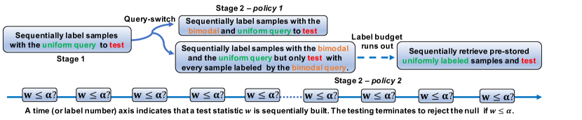
Figure 1: A two-stage active sequential two-sample testing framework. Both policy 1 and 2 alternate between the bimodal and uniform query. Policy 1 updates the test statistic with every sample labeled. In contrast, policy 2 updates the test statistic only with the samples labeled with the bimodal query before the budget runs out and then starts to retrieve the pre-stored uniformly labeled samples to update the test statistic.

A decision maker typically knows little about the difficulty of a two-sample testing problem before running the test. Fixing the sample size to any given value a priori may either result in a test that needs to collect additional evidence to arrive at a final decision (if the problem is hard) or in an inefficient test that has over-collected data (if the problem is simple). To address this dichotomy, the research community proposed sequential two-sample tests [1, 8, 9, 10, 11] that allow the decision maker to sequentially collect data, monitor statistical evidence, i.e., a statistic is computed from the data, and the test can stop anytime when sufficient evidence has been accumulated to make a decision.

Existing sequential two-sample tests [1, 8, 9, 10, 11] are devised to collect both sample features and sample labels simultaneously. This paper considers the sequential two-sample testing problem in a novel practical setting where sample features are inexpensive to access, but sample labels are costly. As a result, the decision maker is allowed to obtain a large collection of sample features and requires the decision maker to sequentially query the label of the samples in this collection to perform the two-sample testing. An immediate application is that doctors validate the dependency between a biomarker ( label variables) and digital test results (feature variables) where the biomarker is expensive to access, and the digital test results are potentially inexpensive replacements for the biomarker; the doctors expect a sequential validation process that uses a reasonable amount of the label budget. Such a design is a special case of the active sequential hypothesis testing elaborated in [12]: A decision maker interacts with the environment and sequentially and actively collects information (sample labels in our case) to test a hypothesis. Existing active sequential hypothesis tests include [12, 13, 14, 15, 16, 17]. However, these works require a clear parametric description of the statistical models of the hypotheses. Although two-sample tests such as the t-test [18] and the Hotelling test [6] assume normality of the feature variables, the problem addressed in our work is a general two-sample independence test, which does not assume a known statistical model.

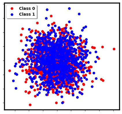
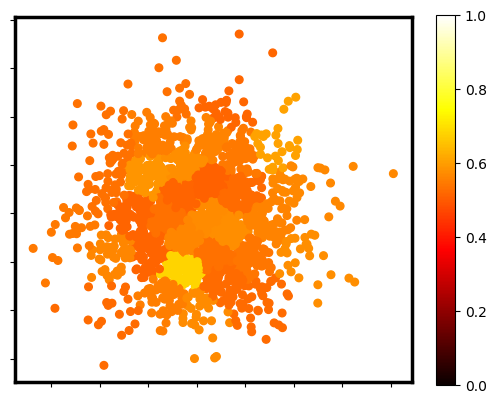
[1pt]Original data [1pt] “Information” map

(a) Case 1

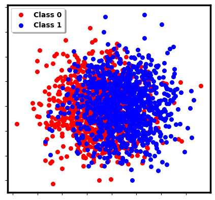
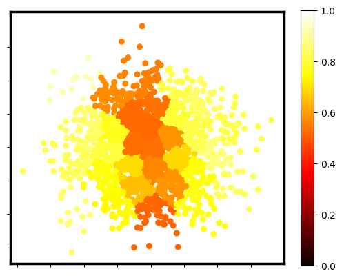
[1pt]Original data [1pt] “Information” map

(b) Case 2

Figure 2: Two data cases under $H_{1}$ and their “information” maps. We compute the “information” maps by partitioning the data into 32 clusters and calculating the proportion of the dominant class samples in a cluster. The brighter color, the more informative samples. Case 1 favors policy 1 as each cluster is similarly informative. Case 2 favors policy 2 as the most distributionally different samples are far more informative than other samples.

This paper proposes the first active sequential two-sample testing framework to test the dependency between the feature variables $S$ and the label variables $Z$ in the setting that a significant number of features realizations $s$ is available but the corresponding label realizations $z$ is expensive to access (See Section 2 for a detailed problem statement). The proposed testing framework is developed based on a likelihood ratio statistic $\prod_{i=1}^{n}\frac{P(z_{i})}{P(z_{i}|s_{i})}$ where $n$ indicates the size of samples participating in the testing so far. Given a feature space $\mathbb{S}$, $P(z)=P(z|s),\forall s\in\mathbb{S}$ and $P(z|s)\neq P(z),\exists s\in\mathbb{S}$ are the statistical models of the two label generation processes, $S\perp\!\!\!\perp Z$ under the null, and $S\not\!\perp\!\!\!\perp Z$ under the alternative hypothesis, respectively. The true $P(z)$ and $P(z\mid s)$ are unknown to a decision maker. We replace $P(z)$ with a prior $\hat{P}(z)$ that maximizes the prior products (likelihood maximization under the null) given the observed labels. In addition, we model $P(z\mid s)$ with a class-probability predictor $Q(z\mid s,\cdot)$. A high-level description of the two-stage testing framework is shown in Figure 1. The framework sequentially builds $w_{n}=\prod_{i=1}^{n}\frac{\hat{P}(z_{i})}{Q_{i}(z_{i}\mid s_{i},\cdot)}$ and rejects the null if $w_{n}$ is smaller than a significance level $\alpha$. Specifically, in the first stage, a decision maker sequentially and uniformly labels samples and construct the test statistic $w$. This stage is an exploration stage in which $Q(z\mid s,\cdot)$ gains enough training samples to guide the selection of informative examples for the second stage. During the second stage, we adopt an active query scheme called the bimodal query [19] to label the samples in regions with high dependency between feature and label variables. We propose one of two policies in the second stage. Both policies alternate between bimodal and uniform queries to label samples sequentially and update $Q(z|s,\cdot)$ with the uniformly labeled samples. However, policy 1 updates $w$ immediately after samples are labeled by the uniform or bimodal query, whereas policy 2 updates $w$ only with the samples labeled by the bimodal query before the label budget runs out. Both policies serve the purpose of producing a small $w$ but are based on different approaches (as selected by a query-switching (QS) scheme): Under Policy 1, the QS scheme predicts that the majority of labeled samples (those acquired via bimodal query and via uniform query) are similarly informative and hence accumulatively multiplies every $\frac{P(z_{i})}{Q_{i}(z_{i}\mid s_{i},\cdot)}$ from both the bimodal and uniform query to produce a small $w$. In contrast, under policy 2 the QS scheme predicts that only the most distributionally different samples are informative so as only to multiply $\frac{P(z_{i})}{Q_{i}(z_{i}\mid s_{i},\cdot)}$ from the bimodal query to generate a small $w$. One of the contributions of this work is a novel QS algorithm that determines when to switch from uniform query (first stage) to active query (second stage) and what policy to use in the second stage. For an intuition about when the QS scheme prefers policy 1 over policy 2 (and vice-versa), we refer the reader to Figure 2 that presents a pictorial case study to illustrate the two policies. We summarize the contributions of our work as follows:

• We devise the first active sequential two-sample testing framework loaded with the two policies following different heuristics.

• We prove that under $H_{0}$, the framework produces an anytime-valid $p$-value to achieve Type I error control. Under $H_{1}$ and reachable conditions and a mild assumption, the framework asymptotically generates a normalized statistic that a passive query can only achieve in the simplest alternative hypothesis where the feature variable and the label variable have the highest dependence (Mutual information $=1$).

• We introduce the QS algorithm to determine when to switch to the second stage and what policy to use in the second stage. While the first stage is proceeding, QS simulates policy 1 and 2 as well as the uniform query by resampling the labeled samples. We compare the simulation results from the three schemes to decide the best parameters to use in the second stage.

• We perform extensive experiments on synthetic data, MNIST, and an application-specific dataset to evaluate the effectiveness of the proposed active sequential test.

Difference from previous work The authors of  [19] devised a label-efficient two-sample test that trains a classifier, uses classifier prediction probabilities to guide the bimodal label query, and performs two-sample testing on the labeled samples. However, their test is a fixed sample size test, and it is unclear when to switch the uniform query to the bimodal query. [8] devised a non-parametric two-sample testing framework. However, their framework is devised to collect both features and labels simultaneously and sequentially. Furthermore, the framework requires a known prior probability of class (label) to construct its statistic. We devise an active sequential two-sample testing framework with a statistic similar to the one in [8] but combined with the bimodal query proposed in [19]. This test has multiple innovations listed in the above contribution section and overcomes the stated limitations of the two tests.

2 Problem Statement and Its Preliminaries

We use a pair of random variables $(S,Z)\in\mathbb{R}^{d}\times\{0,1\}$ to denote a feature variable and its corresponding label variable, and the variable pair admits a joint distribution $p_{SZ}(s,z)$. Formally, a two-sample testing problem consists of null hypothesis $H_{0}$ that states $p_{S\mid Z=0}(s)=p_{S\mid Z=1}(s)$ and an alternative hypothesis $H_{1}$ that states $p_{S\mid Z=0}(s)\neq p_{S\mid Z=1}(s)$. Then, a decision maker collects a sequence $((s,z)_{i})_{i=1}^{N}$ of $N$ realizations of $(S,Z)$ to test $H_{0}$ against $H_{1}$. The problem is equivalent to testing the independency between $S$ and $Z$. Therefore, we declare the following hypotheses for the two-sample testing problem:

$$H_{0}:p_{SZ}(s,z)=p_{S}(s)P_{Z}(z)$$

$$H_{1}:p_{SZ}(s,z)\neq p_{S}(s)P_{Z}(z)$$ (1)

We omit the subscripts in $p_{SZ}(s,z)$, $P_{Z}(z)$ and $p_{S}(s)$ and write them as $p(s,z)$, $P(z)$ and $p(s)$. In addition, we use $s^{N}$, $z^{N}$ and $(s,z)^{N}$ to denote sequences of samples $(s_{i})_{i=1}^{N}$, $(z_{i})_{i=1}^{N}$ and $((s,z)_{i})^{N}_{i=1}$ respectively. We use similar notation throughout the paper.

In the typical setting of a sequential two-sample test, a decision maker does not have prior knowledge of sample features. The decision maker sequentially collects both sample features and their labels simultaneously with the corresponding random variable pair $(S,Z)$ i.i.d. generated from a data-generating process, i.e., $p(s,z)$. We consider a variant of the setting in which accessing sample features is free/inexpensive. Consequently, the decision maker collects a large set $\mathcal{S}_{u}$ of sample features before performing a sequential test. However, accessing the label of a feature in $\mathcal{S}_{u}$ is costly. We assume the following fact throughout the paper: The pre-owned $\mathcal{S}_{u}$ is the result of a sample feature collection process where all $s_{i}\in\mathcal{S}_{u}$ are realizations of random variables $S_{i}$ i.i.d. generated from $p(s)$. There exists an oracle to return a label $z_{i}$ of $s_{i}\in\mathcal{S}_{u}$ with the corresponding random variable $Z_{i}$ and $S_{i}$ admitting the posterior probability $P(z|s)$. We consider the following new sequential two-sample testing problem:

An active sequential two-sample testing problem: Suppose $\mathcal{S}_{u}$ is an unlabeled feature set, there exists an oracle to return a label $z$ of $s\in\mathcal{S}_{u}$, and $N_{q}$ is a limit on the number of times the oracle can be queried (e.g. the label budget). A decision maker sequentially queries the oracle for the $z$ of $s\in\mathcal{S}_{u}$. After querying a new $z_{n}$ of $s_{n}$, for $1\leq n\leq N_{q}$, the decision maker needs to decide whether to terminate the label querying process and make a decision (i.e., whether to reject $H_{0}$) or continue with the querying process if $n<N_{q}$.

A decision maker actively labeling $s_{n}\in\mathcal{S}_{u}$ may result in non-i.i.d pairs of $(S,Z)$, hence the distribution of $(S,Z)$ is shifted away from $p(s,z)$. In contrast, the decision maker passively (or uniformly) labeling $s_{n}\in\mathcal{S}_{u}$ maintains $(S,Z)\sim p(s,z)$. As already generalized in many two-sample testing literature such as [20, 1, 8, 10, 21], a conventional procedure for sequential two-sample testing is to compute a $p$-value from sequentially observed samples and compare it to a pre-defined significance level $\alpha\in[0,1]$ anytime. A decision maker rejects $H_{0}$ and stops the testing if $p\leq\alpha$. We refer readers to [22] for more details. A legitimate sequential two-sample test has the following three attributes:

• The test generates an anytime-valid $p$-value such that, under $H_{0}$, $P_{0}(p\leq\alpha)\leq\alpha$ holds at anytime of the sequential testing process. $P_{0}$ is called a Type I error indicating the probability of making a mistake under the $H_{0}$.

• The test has a high testing power $P_{1}(p\leq\alpha)$ (or low Type II error as Type II error$=1-P_{1}$), which indicates the probability of making a correct decision under $H_{1}$.

• The test is consistent such that $P_{1}(p\leq\alpha)=1$ under $H_{1}$ when the size of test samples goes to infinity.

Bimodal query The authors of [19] proposed the bimodal query to label sample features $s\in\mathbb{S},\mathbb{S}=\operatorname{supp}{(p(s))}$ with the highest $P(Z=0|s)$ or $P(Z=1|s)$. They build a class-probability predictor $Q(z|s,\cdot)$ with uniformly labeled samples to model $P(z\mid s)$. Then, they query the labels of features with the highest $Q(Z=0|s,\cdot)$ or $Q(Z=1|s,\cdot)$ with a fair chance from an unlabeled feature set. A fixed sample size two-sample test in their work constructed by these labeled samples efficiently (in the sense of label query number) reveals the dependency between $S$ and $Z$ when $H_{1}$ is true.

3 A Sequential Two-Sample Testing Statistic

We follow the well-known likelihood ratio test [23] to construct a sequential testing statistic. To achieve this, we use the statistical models that characterize the label generation processes conditional on the observed sample features under $H_{0}$ and $H_{1}$. More precisely, we have the posterior $P(z|s)=P(z)$ to indicate the statistical model under $H_{0}$; this says when $S$ and $Z$ are independent, the posterior probability $P(z|s)$ is the same for any $s$ in the support $\mathbb{S}$ of $p(s)$. In contrast, we have the following statistical model under $H_{1}$: $\exists s\in\mathbb{S},P(z|s)\neq P(z)$. We sequentially collect sample data $(s,z)$, and when a new observation $(s_{n},z_{n})$ arrives, we construct a likelihood ratio $w_{n}$: With $w_{0}=1$, $w_{n}=w_{n-1}\frac{P(z_{n})}{P(z_{n}|s_{n})}=\frac{P(z^{n})}{P(z^{n}\mid s^{n})},n\geq 1$ to assess $H_{0}$ against $H_{1}$. However, the statistical models $P(z)$ and $P(z|s)$ are unknown. We will use a likelihood $\hat{P}(z^{n})$ that is maximized over all the class priors to replace $P(z^{n})$ and build a class-probability predictor $Q_{n}(z\mid s,(s,z)^{t})$ with a past observed sample sequence $(s,z)^{t},t<n$ to model $P(z_{n}\mid s_{n})$. We omit $(s,z)^{t}$ to abbreviate $Q_{n}(z\mid s,(s,z)^{t})$ to $Q_{n}(z\mid s,\cdot)$ and obviously $\sum_{z=0}^{1}Q_{n}(z\mid s,\cdot)=1$. We formally present our sequential testing statistic:

A sequential two-sample testing statistic: Considering $(s,z)$ is sequentially observed, and as a new $(s_{n},z_{n})$ arrives, then, for $n=1,2,\cdots$, a decision maker constructs

$$w_{n}=\frac{\hat{P}(z^{n})}{Q(z^{n}\mid s^{n})}=\prod_{i=1}^{n}\frac{\hat{P}(z_{i})}{Q_{i}(z_{i}\mid s_{i},\cdot)}$$ (2)

where $\hat{P}(Z=1)=\frac{\sum_{i=1}^{n}z_{i}}{n}$ is a class prior chosen to maximize $\hat{P}(z^{n})$ and $Q_{i}(z_{i}\mid s_{i},\cdot)$ is the output of a class-probability predictor built by any past sequence observed before $i$.

We accordingly use $W_{n}$ to indicate a random variable of which $w_{n}$ is a realization. Our test statistic (2) is a generalization of the statistic proposed in [8]. In contrast to that work, our test statistic does not require that the class prior be known, and we devise the statistic to address the practical scenario described in Section 2 where a decision maker has limited access to the label information. The authors of [8] proved that their statistic is an anytime-valid $p$-value; this is also true for our test statistic variant $W_{n}$ used by our testing framework; we formalize this in Section 4.2. A decision maker compares $w_{n}$ with a significance level $\alpha$ for any $n$ and rejects $H_{0}$ if $w_{n}\leq\alpha$. As a result, a small $w_{n}$ is favored under $H_{1}$ to reject $H_{0}$ to endow a sequential two-sample test with the testing power. The class-probability predictor $Q_{i}(z|s,\cdot)$ can be instantiated with classification algorithms such as logistic regression, k-nearest neighbors (KNN), and a support vector machine.

4 Active Sequential Two-Sample Testing

In this section, we propose an active sequential two-sample testing framework that combines the sequential testing statistic in (2) with the bimodal query. Then, we introduce the theorems related to anytime-valid $p$-value and the asymptotic properties. Lastly, we provide the query-switching scheme to determine the parameters to use in the second stage of the proposed framework. We interchangeably use the time to indicate the number of labels progressively queried.

4.1 An Active sequential two-sample testing framework

We propose the active sequential two-sample testing framework shown in Figure 1. Our framework consists of two stages. In the first stage, a decision maker sequentially and uniformly labels samples to update the statistic $w$ (2). In the second stage, the decision maker proceeds either with policy 1 or 2 to alternatively take $M^{1}$ steps of the bimodal query and $M^{2}$ steps of the uniform query (i.e. $M^{1}$ bimodal queries$\to$$M^{2}$ uniform queries$\to$$M^{1}$ bimodal queries$\to$$M^{2}$ uniform queries$\cdots$) to label samples sequentially to update $w$. Policy 1 updates $w$ after querying a new label with the bimodal query or uniform query. Policy 2 updates $w$ only using the samples labeled by the bimodal query, and the uniformly labeled samples are stored; when the label budget runs out, it starts retrieving the uniformly labeled samples to update $w$. In both stages, the decision maker sequentially builds $w$, updates the class-probability predictor $Q(z|s,\cdot)$ only with samples labeled by the uniform query, and rejects $H_{0}$ if $w\leq\alpha$.

To precisely introduce our framework, we use the following notations. We write $\mathcal{S}_{u}$ to denote an unlabeled feature set, write $\mathcal{S}_{w}$ to denote a labeled feature sequence collected from the uniform query, write $\mathcal{Z}_{w}$ to denote the corresponding label sequence, and $\mathcal{S}_{q}$ to denote a sequence of all labeled features. In addition, we write $\mathcal{S}^{*}_{u}$ to denote a set of features that the uniform query has not visited. $\mathcal{S}^{*}_{u}$ is a feature collection that remained after the original feature set (Combines $\mathcal{S}_{u}$ and $\mathcal{S}_{q}$) with $\mathcal{S}_{w}$ uniformly sampled out. This says, $S$ in $\mathcal{S}^{*}_{u}$ and $\mathcal{S}_{u}$ both follow $p(s)$. A decision maker uses the bimodal query on $\mathcal{S}_{u}$ to label features that are most distributionally different, whereas he/she uses the uniform query on $\mathcal{S}^{*}_{u}$ to ensure every uniformly queried $(S,Z)$ follows $p(s,z)$. Such design serves the purpose of producing an anytime-valid $p$-value (see Section 4.2). Since accumulating $(z_{i},Q_{i}(z_{i}|s_{i},\cdot))$ from a labeled sample leads to the test statistic (2), we call each $(z_{i},Q_{i}(z_{i}|s_{i},\cdot))$ by the name test unit. We use $\mathcal{R}_{0}=((z_{i},Q_{i}(z_{i}|s_{i},\cdot)))_{i=1}^{n_{0}}$ to denote a test unit sequence that collects the test units immediately used to build $w$, e.g. $(z_{i},Q_{i}(z_{i}|s_{i},\cdot))$ from the bimodal and uniform query in stage 2–policy 1. Similarly, we use $\mathcal{R}_{1}=((z_{i},Q_{i}(z_{i}|s_{i},\cdot)))_{i=1}^{n_{1}}$ to denote a backup test unit sequence that stores the test units from the uniform query stage 2–policy 2, as these test units are not used to build $w$ until the label budget runs out. In the following, we introduce each stage of our framework, supposing a decision maker will query the $n^{\text{th}}$ new label next for $n\in[1,N_{q}]$. We omit $i$ in $Q_{i}(z|s,\cdot)$ and use $Q(z|s,\cdot)$ to represent the latest class-probability predictor.

• First stage Continuously perform uniform query operation¹ until $H_{0}$ is rejected, the label budget runs out or the decision maker decides to enter the second stage.

• Second stage – policy 1: Alternatively perform $M^{1}$ steps of bimodal query operation and $M^{2}$ steps of uniform query operation¹.

• Second stage – policy 2: Alternatively perform $M^{1}$ steps of bimodal query operation and $M^{2}$ steps of uniform query operation²; if the label budget is exhausted, perform the retrieval operation.

• The bimodal query operation: Label $z_{n}$ of a sample $s_{n}$ from $\mathcal{S}_{u}$ by the bimodal query. Add $(z_{n},Q(z_{n}\mid s_{n},\cdot))$ to $\mathcal{R}_{0}$. Construct the test statistic $w_{n_{0}}$ with $\mathcal{R}_{0}$ and compare it with $\alpha$. Update $\mathcal{S}_{u},\mathcal{S}_{q},\mathcal{S}_{u}^{*}$.

• The uniform query operation¹: Uniformly sample $s_{n}$ from $\mathcal{S}_{u}^{*}$. If $z_{n}$ of $s_{n}$ is not queried, query $z_{n}$, add $(z_{n},Q(z_{n}\mid s_{n},\cdot))$ to $\mathcal{R}_{0}$, and construct the test statistic $w_{n_{0}}$ with $\mathcal{R}_{0}$ and compare it with $\alpha$. Update $\mathcal{S}_{u},\mathcal{S}_{w},\mathcal{S}_{q},\mathcal{Z}_{w},\mathcal{S}_{u}^{*}$; update $Q(z\mid s,\cdot)$ with $\mathcal{S}_{w}$ and $\mathcal{Z}_{w}$.

• The uniform query operation²: Uniformly sample $s_{n}$ from $\mathcal{S}_{u}^{*}$. If $z_{n}$ of $s_{n}$ is not queried, query $z_{n}$ and add $(z_{n},Q(z_{n}\mid s_{n},\cdot))$ to $\mathcal{R}_{1}$. Update $\mathcal{S}_{u},\mathcal{S}_{w},\mathcal{S}_{q},\mathcal{Z}_{w},\mathcal{S}_{u}^{*}$. Update $Q(z\mid s,\cdot)$ with $\mathcal{S}_{w}$ and $\mathcal{Z}_{w}$.

• The retrieval operation: Remove the first element $r_{1}$ from $\mathcal{R}_{1}$ and add $r_{1}$ to $\mathcal{R}_{0}$. Construct the test statistic $w_{n_{0}}$ with $\mathcal{R}_{0}$ and compare it with $\alpha$.

The uniform query operations need to verify if the selected feature is labeled, as some features of $\mathcal{S}^{*}_{u}$ might already be labeled by the bimodal query. The two policies adopt different heuristics. Policy 1 constructs the test statistic with $\mathcal{R}_{0}$ in which $(z_{i},Q_{i}(z_{i}\mid s_{i},\cdot))$ is immediately returned after a sample is labeled by the bimodal query or the uniform query, under the assumption that more test samples lead to a higher testing power. In contrast, policy 2 only adds $(z_{i},Q_{i}(z_{i}\mid s_{i},\cdot))$ returned by the bimodal query to $\mathcal{R}_{0}$ immediately to construct test statistic. Only if the label budget is exhausted, and $H_{0}$ is not rejected, does the policy 2 starts to retrieve $(z_{i},Q_{i}(z_{i}\mid s_{i}\cdot))$ from $\mathcal{R}_{1}$ to construct the test statistic. Policy 2 is based on including only the most distributionally different samples in the two-sample to maximize testing power. The retrieval operation in policy 2 uses the stored uniformly labeled samples that have not participated in the testing to update the test statistic when the label budget runs out, and $H_{0}$ is not rejected, in order to exploit the statistical evidence in the unused uniformly labeled samples. With these preliminaries, we formally introduce our active sequential two-sample testing framework.

An active sequential two-sample testing framework: Suppose $N_{q}$ is a label budget and $\alpha$ is a significance level. A decision maker uses the proposed framework that switches to either policy 1 or 2 at some query-switching time $N_{sw}$ with the step sizes $M^{1}$ and $M^{2}$ to sequentially build the test unit sequence $\mathcal{R}_{0}$. As the $n_{0}^{\text{th}}$ $(z_{n_{0}},Q(z_{n_{0}}|s_{n_{0}},\cdot))$ is added to $\mathcal{R}_{0}$, then for $1\leq n_{0}\leq N_{q}$, we construct the following statistic with $\mathcal{R}_{0}=((z_{i},Q_{i}(z_{i}\mid s_{i},\cdot)))_{i=1}^{n_{0}}$

$$w_{n_{0}}=\prod_{i=1}^{n_{0}}\frac{\hat{P}(z_{i})}{Q_{i}(z_{i}\mid s_{i},\cdot)}.$$ (3)

$H_{0}$ is rejected if $w_{n_{0}}\leq\alpha$ or not rejected if $n_{0}=N_{q}$, otherwise the test continues.

There are several design parameters in the test, including at what time $N_{sw}$ to switch, which policy should be used, and what values of $M^{1}$ and $M^{2}$ should be used. In Section 4.4, we will propose a practical query-switching algorithm that helps a decision maker decide on these parameters.

4.2 The proposed framework controls the Type I error

Our framework rejects $H_{0}$ if the statistic $w_{n_{0}}\leq\alpha$ (3).The following theorem states that under $H_{0}$, $w_{n_{0}}$ is an anytime-valid $p$-value.

Theorem 4.1.

Suppose $N_{q}$ is a label budget, and $\alpha$ is a significance level. A decision maker uses the proposed framework to sequentially query the oracle for $Z$ of $S\in\mathcal{S}_{u}$ resulting in $\mathcal{R}_{0}=((Z_{i},Q_{i}(Z_{i}|S_{i},\cdot)))_{i=1}^{N_{0}}$. Then for $1\leq N_{0}\leq N_{q}$, we have the following under $H_{0}$,

$$P_{0}\left(\exists N_{0},W_{N_{0}}=\prod_{i=1}^{N_{0}}\frac{\hat{P}(Z_{i})}{Q_{i}(Z_{i}\mid S_{i},\cdot)}\leq\alpha\right)\leq\alpha$$ (4)

Theorem 4.1 implies the probability $P_{0}$ (or Type I error) that our framework mistakenly rejects $H_{0}$ is upper-bounded by $\alpha$. The sketch of the proof for Theorem 4.1 is as follows: The decision maker updates $Q_{i}(z|s,\cdot)$ only with past observations collected from the uniform query. It ensures that no label realizations of $Z_{i}$ for $S_{i}\in\mathcal{S}_{u}$ leak to the decision maker. Therefore, $\forall S\in\mathcal{S}_{u}$ and the newly queried $Z$ is independent under $H_{0}$. Furthermore, as $\prod_{i=1}^{N_{0}}\hat{P}(Z_{i})$ is a likelihood maximized over class priors, we use the Ville’s maximum inequality [24, 25] to develop Theorem 4.1. We refer readers to Appendix A.2 for complete proof.

4.3 Asymptotic properties of the proposed framework

Policy 1 and 2 both use the bimodal query to label samples, and $H_{0}$ and $H_{1}$ can be differentiated faster by constructing a small $w_{n_{0}}$ (3) with the labeled samples under $H_{1}$. In the following, we prove that both policies generate a normalized $w_{n_{0}}$ which asymptotically approaches the minimum that a uniform query can only achieve under the simplest $H_{1}$ (i.e. when the feature variable and the label variable have the highest mutual information). Before that, we first define two concepts:

Definition 1.

($\lambda$- hard) $H_{1}$ is a $\lambda$- hard alternative hypothesis if the mutual information (MI) $I(S,Z)=1-\lambda,\forall\lambda\in[0,1)$.

MI is well-known to measure the dependency between features and labels [26]. Under the null $H_{0}$, $I(S,Z)=0$, and under the alternative $H_{1}$, $I(S,Z)>0$. Therefore, $I(S,Z)$ reflects how much $H_{1}$ deviates from $H_{0}$. As a result, in Definition 1, we naturally use $I(S,Z)$ to measure the intrinsic difficulty of detecting $H_{1}$ by the two-sample testing if $H_{1}$ is true.

Definition 2.

$Q_{i}(z|s,\cdot)$ is a pointwise consistent class-probability predictor (p.c.c.p) if $\lim_{i\to\infty}Q_{i}(z|s,\cdot)\to P(z|s)$.

Suppose there is a sequence $(S,Z)^{N}$ with every $(S,Z)$ i.i.d. generated from $p(s,z)$. The authors of [8] and [27] suggest that $Q(z|s,(S,Z)^{N})$ constructed by partitioning, kernel, and nearest neighbor estimates of $P(z|s)$ achieves the point-wise consistency defined in 2 with proper scales (e.g. number of nearest neighbors) as $N$ goes to infinity. We need to make one additional assumption before stating the final result as follows,

Assumption 4.2.

Suppose $\mathbb{S}$ is the support of $p(s)$. Under $H_{1}$, there exists regions $\mathbb{S}_{0}\subset\mathbb{S}$ and $\mathbb{S}_{1}\subset\mathbb{S}$ such that $P(Z=0|s)=1,\forall s\in\mathbb{S}_{0}$ and $P(Z=1|s)=1,\forall s\in\mathbb{S}_{1}$.

Assumption 4.2 states that under $H_{1}$ there are at least two regions with absolute class prediction $p(z|s)=1$ for class 0 and 1. The same assumption was used in [28] to address a nearest neighbor classification problem.

Now, we introduce the asymptotic property of our framework. Considering a test statistic unit sequence $\mathcal{R}_{0}$ built by the policy 1 or 2 in the second stage of our framework, a normalized version $\overline{W}^{q}_{N_{0}}$ of the test statistic in (3) is expressed as $\overline{W}^{q}_{N_{0}}=\frac{1}{N_{0}}\sum_{i=1}^{N_{0}}\log\frac{\hat{P}(Z_{i})}{Q_{i}(Z_{i}\mid S_{i},\cdot)}$ with each $(Z_{i},Q_{i}(Z_{i}\mid S_{i},\cdot))$ is an element of $\mathcal{R}_{0}=((Z_{i},Q_{i}(Z_{i}\mid S_{i},\cdot)))_{i=1}^{N_{0}}$. Similarly, we use $\overline{W}^{p}_{N_{p}}$ to indicate the same normalized statistic produced by a passive (or uniform) query scheme. It is completely constructed from $\{S,Z\}^{N_{p}}$ with its labels sequentially and uniformly queried: $\overline{W}^{p}_{N_{p}}=\frac{1}{N_{p}}\sum_{i=1}^{N_{p}}\log\frac{\hat{P}(Z_{i})}{Q_{i}(Z_{i}\mid S_{i},\cdot)},\forall(S_{i},Z_{i})\sim p(s,z)$. We compare $\overline{W}^{q}_{N_{0}}$ to $\overline{W}^{p}_{N_{p}}$ and introduce the following:

Theorem 4.3.

Suppose a decision maker uses the framework with a p.c.c.p. $Q_{i}(z|s,\cdot)$, and with the step sizes $M^{1}$ and $M^{2}$ having $\lim_{N_{0}\to\infty}\frac{M^{2}}{M^{1}}\to 0$. Then, under Assumption 4.2, we have the following under $H_{1}$,

$$\lim_{N_{p}\to\infty}\overline{W}^{p}_{N_{p}} \to-(H(Z)-H(Z|S))=-I(S,Z)$$

$$\hskip 71.13188pt\quad(S,Z)\sim p(s,z)$$ (5)

$$\lim_{N_{0}\to\infty}\overline{W}^{q}_{N_{0}} \to-(H^{*}(Z)-H^{*}(Z|S))=-I^{*}(S,Z)$$

$$=-1,\quad(S,Z)\sim p^{*}(s,z)$$ (6)

where $I(S,Z)$ is MI resulting from original $H_{1}$ that is $1-I(S,Z)$ hard, and $I^{*}(S,Z)$ is MI constructed with $(S,Z)\sim p^{*}(s,z)$ which is a joint distribution corresponding to the $0$-hard $H_{1}$ ($I^{*}(S,Z)=1$).

We brief the proof of Theorem 4.3 in the following: As $Q_{i}(z|s,\cdot)$ asympotically converges to the true $P(z|s)$ and both policy 1 and 2 only label features with highest $Q_{i}(0|s,\cdot)$ and $Q_{i}(1|s,\cdot)$, when $N_{0}$ is very large, with Assumption 4.2 made, our framework asymptotically modifies the joint distribution of $(S,Z)$ to $p^{*}(s,z)$ by only labelling samples in $\mathbb{S}_{0}$ and $\mathbb{S}_{1}$ where $P(0|s)=1,\forall s\in\mathbb{S}_{0}$ and $P(1|s)=1,\forall s\in\mathbb{S}_{1}$, resulting to $-\overline{W}^{q}_{N_{0}}=I^{*}(S,Z)=1,(S,Z)\sim p^{*}(s,z)$. In contrast, the asymptotic value of $-\overline{W}^{p}_{N_{p}}$ from the uniform query remains as $I(S,Z)$ with $(S,Z)\sim p(s,z)$ and $p(s,z)$ is the original distribution. Please refer to Appendix A.3 for complete proof.

Remark 1.

Theorem 4.3 states that $\overline{W}^{p}_{N_{p}}$ constructed with the uniform label query converges to $-I(S,Z)$ determined by the original $p(s,z)$. In contrast, our framework asymptotically leads to $\overline{W}^{q}_{N_{0}}=-1$, which is a lower bound of $-I(S,Z)=-(H(Z)-H(Z|S))\geq-(1-0)=-1$. This equivalently says that, under $H_{1}$, our framework converts the original $\lambda_{p}$-hard $H_{1}$ to the simplest $0$-hard $H_{1}$

Theorem 4.4.

Under $H_{1}$ and the same conditions of Theorem 4.3, the proposed testing framework is also consistent as

$$\lim_{N_{0}\to\infty}P_{1}\left(\prod_{i=1}^{N_{0}}\frac{\hat{P}(Z_{i})}{Q_{i}(Z_{i}\mid S_{i},\cdot)}\leq\alpha\right)=\lim_{N_{0}\to\infty}P(\overline{W}^{q}_{N_{0}}\leq\frac{1}{N_{0}}\log(\alpha))=P_{1}(-1\leq 0)=1$$ (7)

We refer readers to Appendix A.4 for the elaborated proof.

4.4 Query-switching

In this section, we propose a query-switching (QS) algorithm and refer readers to Algorithm 1 in Appendix for the algorithmic details. During the first stage of our framework, QS simulates policy 1 and 2 as well as the uniform query by resampling the labeled samples, thereby resulting in collections of the statistic from the three schemes. We compare the statistic means of the collections from the uniform query, policy 1 and 2 to decide what time $N_{sw}$ to switch to stage 2, what policy to use, and what step sizes $M^{1}$ and $M^{2}$ of the queries to use in the second stage.

In the first stage, a decision maker periodically uses the QS algorithm for every $T_{sw}$ label query, and $T_{sw}$ is a pre-selected parameter. For instance, after $n=T_{sw}$ uniform label queries in the first stage, the QS algorithm takes the following inputs: A uniformly labeled sample features sequence $(s_{i})_{i=1}^{n}$, the corresponding label sequence $(z_{i})_{i=1}^{n}$, a class-probability predictor sequence $(Q_{i}(z|s,\cdot))_{i=1}^{n}$ and a candidate set of step sizes $\{(M^{1},M^{2})_{i}\}_{i=1}^{L}$. Then, the QS algorithm randomly generates a set of index $\mathcal{T}=\{t_{1},\cdots,t_{I}\},\forall t\in\mathcal{T},1\leq t<n$ and each $t\in\mathcal{T}$ indicates an element index for the sequences $(s_{i})_{i=1}^{n}$, $(z_{i})_{i=1}^{n}$ and $(Q_{i}(z|s,\cdot))_{i=1}^{n}$. Subsequently, elements in these sequences with the index from $t\in\mathcal{T}$ to the end are used to form $I$ subsequences $(s_{i})_{i=t}^{n}$, $(z_{i})_{i=t}^{n}$ and $(Q_{i}(z|s,\cdot))_{i=t}^{n},\forall t\in\mathcal{T}$. We use these subsequences to evaluate the statistics (3) generated from the uniform query, policies 1 and 2 with $L$ different step sizes $M^{1}$ and $M^{2}$. As we will see, these statistics do not participate in the two-sample testing and are only used to predict and compare the performance of the uniform query and the two policies. Thus we call them QS statistics. Suppose there are $N_{u}$ unlabeled samples remaining, and the current label budget is $N_{q}$. The decision maker uses $I$ recorded $(s_{i})_{i=t}^{n},(z_{i})_{i=t}^{n}$ and $(Q_{i}(z|s,\cdot))_{i=t}^{n},\forall t\in\mathcal{T}$ to simulate the uniform query, policy 1 and 2 with different step sizes assuming a label budget of $(n-t+1)\frac{N_{q}}{N_{u}}$ to generate the QS statistics. Next, obtain the QS statistic means of the $I$ QS statistics for the uniform query, policy 1 and 2. The decision maker either remains in the first stage if the uniform QS statistic mean is the smallest or enters the second stage by switching to the policy with $(M^{1},M^{2})\in\{(M^{1},M^{2})_{i}\}_{i=1}^{L}$ that generates the smallest QS statistic mean. Our QS scheme is a variation on bootstrapping [29] since it repeatedly draws samples from a population to estimate a population parameter. The difference is that our QS scheme resamples a subsequence segment from a random starting index to the end of the original sequence. It provides the benefit of reusing past class-probability predictors such that there is no need to rebuild them and that newer $Q_{i}(z\mid s,\cdot)$’s have higher chance to participate in the decision of QS.

Algorithm 1 Query-switching

1:Input: $(s_{i})_{i=1}^{n},(z_{i})_{i=1}^{n},(Q_{i}(z|s,\cdot))_{i=1}^{n},$

2:$\{(M^{1},M^{2})_{i}\}_{i=1}^{L},N_{q},N_{u},I$

3:Output: Stay in stage 1 or enter stage 2 with a selected policy with proper $M^{1}$ and $M^{2}$.

4:Initialization: Set $W^{u}$, all $W^{1}$ in $(W^{1}_{i})_{i=1}^{L}$ and all $W^{2}$ in $(W^{2}_{i})_{i=1}^{L}$ to zero, and set the ratio of the label budget $N_{q}$ to the unlabeled sample number $N_{u}$ to $r=\frac{N_{q}}{N_{u}}$

5:for $T=1,\cdots,I$ do

6:     Sample an element $t$ from $[1,n)$

7:     Get subsequences $(s_{i})_{i=t}^{n},(z_{i})_{i=t}^{n},(Q_{i}(z|s,\cdot))_{i=t}^{n}$

8:     Set a label budget $N_{q}^{{}^{\prime}}=\lfloor(n-t+1)*r\rfloor$ in terms of the subsequence length $n-t+1$

9:     Compute the QS statistics $w^{u}$, $(w^{1}_{i})_{i=1}^{L}$ and $(w^{2}_{i})_{i=1}^{L}$ by applying the uniform query, policy 1 and policy 2 with all $(M^{1},M^{2})\in\{(M^{1},M^{2})_{i}\}_{i=1}^{L}$ respectively to the subsequences $(s_{i})_{i=t}^{n}$, $(z_{i})_{i=t}^{n}$, and $(Q_{i}(z|s,\cdot))_{i=t}^{n}$ for the label budget $N_{q}^{{}^{\prime}}$.

10:     Use element-wise addition to add the resulting $w^{u}$ to $W^{u}$, $(w^{1}_{i})_{i=1}^{L}$ to $(W^{1}_{i})_{i=1}^{L}$ and $(w^{2}_{i})_{i=1}^{L}$ to $(W^{2}_{i})_{i=1}^{L}$

11:end for

12:Divide $W^{u},(W^{1}_{i})_{i=1}^{L},(W^{2}_{i})_{i=1}^{L}$ by $I$ respectively to get the QS statistic means:$\bar{W}^{u},(\bar{W}^{1}_{i})_{i=1}^{L},(\bar{W}^{2}_{i})_{i=1}^{L}$

13:Compare $\bar{W}^{u},(\bar{W}^{1}_{i})_{i=1}^{L},(\bar{W}^{2}_{i})_{i=1}^{L}$

14:Return: Stay in stage 1 if $\bar{W}^{u}$ is the smallest, or enter stage 2 with policy 1 with $M^{1}_{i}$ and $M^{2}_{i}$ if $\bar{W}^{1}_{i}$ from $(\bar{W}^{1}_{i})_{i=1}^{L}$ is the smallest, or with policy 2 with $M^{1}_{i}$ and $M^{2}_{i}$ if $\bar{W}^{2}_{i}$ from $(\bar{W}^{2}_{i})_{i=1}^{L}$ is the smallest

5 Experimental Results

Implementing the proposed active sequential two-sample testing framework with the QS algorithm requires setting up the following five hyper-parameters: A period $T_{sw}$ of using the QS algorithm in the first stage, a set of step sizes $(M^{1},M^{2})$ from which QS can select, an algorithm $\mathcal{A}$ to construct the class-probability predictor $Q(z\mid s,\cdot)$, the size $N_{0}$ of samples to initialize $Q(z\mid s,\cdot)$ and a significance level $\alpha$. We refer readers to Algorithm 2 in Appendix for full algorithmic details. We compare our framework with a sequential testing baseline designed by modifying the sequential test in [8] to evaluate our proposed framework fairly. As the authors of [8] devise their framework assuming the class priors are known, we replace their statistic with our statistic in (2) that addresses the unknown class priors scenario to build our sequential testing baseline. This baseline is a standard sequential two-sample test that passively labels samples. In addition, we use our framework to build another two tests that perform Policy 1 and Policy 2, respectively, from the beginning of the testing without QS. This is to verify the effectiveness of the proposed QS algorithm. We perform our experiments on synthetic datasets, MNIST and Alzheimer’s Disease Neuroimaging Initiative (ADNI) database [30]. We set $T_{sw}=100$ and set $(M^{1},M^{2})$ to $\{(3,1),(2,1),(1,1),(1,2),(1,3)\}$ and $\{(5,1),(4,1),(3,1),(2,1),(1,1)\}$ respectively. We build $Q(z\mid s,\cdot)$ with logistic regression, SVM, or KNN classifiers and set $N_{0}=10$ and $\alpha=0.05$. We present the representative experimental results with the following notations: Baseline – A passive sequential two-sample test [8]. Ours-NoQS¹/Ours-NoQS² – Proposed testing frameworks with policy 1/policy 2 used at the beginning without QS. Ours-QS¹/Ours-QS² – Proposed testing frameworks combined with QS with the two candidate step sets $\{(M^{1},M^{2})_{i}\}_{i=1}^{L}$.

Label budget	200	400	600	800	1000
Baseline	0.83	0.53	0.30	0.11	0.04
Ours-NoQS1	0.55	0.35	0.26	0.19	0.14
Ours-NoQS2	0.50	0.35	0.26	0.19	0.14
Ours-QS1	0.50	0.16	0.04	0.01	0.02
Ours-QS2	0.50	0.16	0.07	0.03	0.03

Table 1: Type II errors of the proposed tests and the baseline test [8] with different label budgets.

$\delta$	0.5	0.4	0.3	0.2
Baseline	63.90	101.02	178.28	451.37
Ours-QS1	63.63	87.67	127.72	271.12
Ours-QS2	63.64	88.18	131.10	276.00

Table 2: Avg. stopping times of the proposed tests and the baseline test [8] for a fixed label budget of 1000.

Label budget	200	400	600	800	1000
Synthetic dataset
Ours-QS1	0.010	0.008	0.010	0.008	0.012
Ours-QS2	0.008	0.012	0.008	0.008	0.012
MNIST
Ours-QS1	0.020	0.020	0.020	0.020	0.020
Ours-QS2	0.020	0.020	0.020	0.020	0.020

Table 3: Type I errors of the proposed tests for different label budgets $N_{q}$ are upper-bounded by $\alpha=0.05$.

5.1 Experiments on synthetic datasets

We create binary synthetic datasets with sample features generated from $p(s\mid Z=0)\equiv\mathcal{N}\left((-\delta,0),I\right)$ and $p(s\mid Z=1)\equiv\mathcal{N}\left((\delta,0),I\right)$ for two classes. We set $P(Z=0)$ from $0.5$ to $0.8$ to vary the ratio of the class zero sample size to the others. We set $\delta=0$ to create the datasets for $H_{0}$, and vary $\delta$ from $0.2$ to $0.5$ to create the datasets for $H_{1}$. All generated datasets are of size 2000. We apply the same choice of hyper-parameter setup for our proposed test and the sequential testing baseline. We ran the tests on the 200 synthetic datasets randomly generated and averaged the generated results. Herein, we present the Type II errors for the sequential tests with the logistic regression used on the dataset with $\delta=0.2$ and $P(Z=0)=0.5$ for $H_{1}$.

Table 1 shows that our active sequential two-sample test combined with the QS algorithm achieves the lowest Type II error rate with a smaller label budget by sequentially and actively labeling samples. Furthermore, we compare our average test-stopping time for datasets of increasing difficulties. More specifically, we vary $\delta$ from $0.5$ to $0.2$ and generate Type II errors with a fixed label budget of 1000. As shown in Table 2, the average test-stopping time of our test increases with decreasing $\delta$ (increasing problem difficulties). It implies that our sequential testing adaptively collects more data to test $H_{0}$ and $H_{1}$ when a considered two-sample testing problem is hard.

Lastly, we implement the proposed active sequential two-sample test on the dataset with $\delta=0$. For this case, $H_{0}$ is true, and we ran the test 500 times on the dataset for $P(Z=0)=0.5$ to generate the Type I error. Table 3 presents the Type I error of the proposed test performed on the dataset with $P(Z=0)=0.5$. We observe that the Type I error is upper-bounded by $\alpha=0.05$, which agrees with Theorem 4.1.

6 Experiments on MNIST and ADNI

$N_{q}$	Methods	Type II error	Stopping time
200	Baseline	0.59	160.85
	Ours-NoQS1	0.51	134.33
	Ours-NoQS2	0.55	133.58
	Ours-QS1	0.27	145.20
	Ours-QS2	0.31	146.46
400	Baseline	0.16	233.20
	Ours-NoQS1	0.23	204.24
	Ours-NoQS2	0.33	223.51
	Ours-QS1	0.02	172.92
	Ours-QS2	0.01	175.59
600	Baseline	0.02	247.46
	Ours-NoQS1	0.07	229.70
	Ours-NoQS2	0.17	270.83
	Ours-QS1	0.01	175.08
	Ours-QS2	0.01	178.82
800	Baseline	0.01	249.27
	Ours-NoQS1	0.02	237.27
	Ours-NoQS2	0.09	293.77
	Ours-QS1	0.00	176.66
	Ours-QS2	0.00	180.32
1000	Baseline	0.01	250.27
	Ours-NoQS1	0.02	241.27
	Ours-NoQS2	0.07	308.05
	Ours-QS1	0.00	173.33
	Ours-QS2	0.00	183.50

$N_{q}$	Methods	Type II error	Stopping time
200	Baseline	0.11	95.58
	Ours-NoQS1	0.33	59.93
	Ours-NoQS2	0.11	74.09
	Ours-QS1	0.04	85.96
	Ours-QS2	0.05	74.09
300	Baseline	0.01	100.89
	Ours-NoQS1	0.10	64.20
	Ours-NoQS2	0.09	83.72
	Ours-QS1	0.00	86.56
	Ours-QS2	0.01	87.37
400	Baseline	0.00	101.15
	Ours-NoQS1	0.04	65.20
	Ours-NoQS2	0.04	90.67
	Ours-QS1	0.00	86.09
	Ours-QS2	0.01	87.96
500	Baseline	0.00	101.15
	Ours-NoQS1	0.04	65.20
	Ours-NoQS2	0.03	94.53
	Ours-QS1	0.00	87.63
	Ours-QS2	0.00	87.75
600	Baseline	0.00	101.15
	Ours-NoQS1	0.04	65.20
	Ours-NoQS2	0.02	96.70
	Ours-QS1	0.00	85.67
	Ours-QS2	0.00	87.96

Table 4: Type II errors and Avg. stopping times of the proposed tests and the baseline test [8] for MNIST (Left, $P(Z=0)=0.6$) and ADNI (Right, $P(Z=0)=0.7$).

MNIST under $H_{0}$ and $H_{1}$: We randomly sample 2000 images from one digit category and label them class zero. We randomly sample another 1400 images from the same category and 600 images from another category. We label these samples as class one. We resample data in class zero ($Z=0$) and one ($Z=1$) to simulate priors $P(Z=0)$ ranging from 0.5 to 0.8. Similarly, we simulate data under $H_{0}$, except that the class zero samples and the class one samples both come from the same digit category. Instead of using the raw input samples, we projected the MNIST data to a 28-dimensional space by a convolutional autoencoder. We produce 200 MNIST two-sample datasets with a size of 2000 for $H_{1}$ and 500 two-sample datasets for $H_{1}$ for different $P(Z=0)$. The Alzheimer’s Disease Neuroimaging Initiative (ADNI) dataset under $H_{1}$: We use the ADNI database [30] to demonstrate a real-world application of the proposed test. The motivation for these results stems from a desire for doctors to replace an expensive Alzheimer’s biomarker with digital test results that are inexpensive to obtain. In this experiment, we evaluate the dependency between the binarized (expensive) biomarker variable (or the label variable) $Z$ and the digital test result variable (or the feature variable) $S$. Evaluating the biomarker $Z$ with CT scans is expensive; hence a statistician assigns a label budget to the two-sample test; we use the proposed test and a fixed label budget for evaluation. We create 200 ADNI two-sample datasets with a size of 1000 for each $P(Z=0)$ from $0.5$ to $0.8$.

We implement the proposed test with the hyper-parameters stated in the first paragraph in Section 5. Table 4 shows the Type II errors generated by using the logistic regression in our testing framework on the MNIST and ADNI two-sample data. We observe that the proposed tests with QS consistently generate lower or equivalent Type II errors compared to other tests for every label budget. Table 4 also presents the corresponding test-stopping times. As observed, our tests reject $H_{0}$ with fewer label queries for all label budgets, which agrees with our Theorem 4.3 that implies the proposed framework tends to generate a small statistic favorable to rejecting $H_{0}$. The proposed tests without QS could lead to a smaller average stopping time, as policy 1 or 2 has been used since the beginning; however, the resulting Type II errors could be higher than the baseline, as there is no QS to decide which policy to use and when to use. Lastly, we produce the Type I error of the proposed test performed on the MNIST two-sample data under $H_{0}$. Table 3 shows that the Type I of our test is upper-bounded by $\alpha=0.05$.

7 Conclusion

We propose an active sequential two-sample hypothesis testing framework capable of sequentially and actively labeling the samples. Experimental results demonstrate the effectiveness of the framework combined with query-switching.

Appendix A Proofs

A.1 Some statistical preliminaries

In probability theory, a sequence of random variables is called martingale if the conditional expectation of the next random variable in the sequence is the expected value of the present random variable. In other words, the conditional expectation of the next random variable only depends on the values of the present variable regardless of past variables in the sequence. The proof of Theorem 4.1 involves theory related to the martingale. We refer interested readers to [31] for an introduction to martingale and related theories. In the following, we present a bare minimum we need for developing Theorem 4.1.

Definition 3.

(Martingale) A sequence of random variables $X_{0},X_{1},\cdots$ is a martingale if, for any $n\geq 0$,

$$\mathop{\mathbb{E}}[|X_{n}|] \leq\infty$$ (8)

$$\mathop{\mathbb{E}}[X_{n+1}|X_{1},X_{2},\cdots,X_{n}] =X_{n}$$ (9)

Theorem A.1.

[32]: If $(X_{n})$ is a nonnegative martingale, then for any $c>0$, we have

$$P\left(\sup_{n\in\mathbb{N}}X_{n}>x\right)\leq\frac{\mathop{\mathbb{E}}[X_{0}]}{c}$$ (10)

A.2 Proof of Theorem 4.1

Proof.

Our framework sequentially and actively queries label $z$ of a feature $s\in\mathcal{S}_{u}$. Our proof consists of two ordered parts: (1) Under the null hypothesis $H_{0}$, the random variables $S$ and $Z$ corresponding to the feature realization $s$ and its label realization $z$ queried in the framework are independent. (2) Under the null, with $\mathcal{R}_{0}=((Z_{i},Q_{i}(Z_{i}\mid S_{i},\cdot)))_{i=1}^{N_{0}}$, we have $P_{0}\left(\exists N_{0},W_{N_{0}}=\prod_{i=1}^{N_{0}}\frac{\hat{P}(Z_{i})}{Q_{i}(Z_{i}\mid S_{i},\cdot)}\leq\alpha\right)\leq P_{0}\left(\exists N_{0},\tilde{W}_{N_{0}}=\prod_{i=1}^{N_{0}}\frac{P(Z_{i})}{Q_{i}(Z_{i}\mid S_{i},\cdot)}\leq\alpha\right)\leq\alpha$
$S$ and $Z$ are independent under $H_{0}$: We use $((\mathcal{S}_{u})_{i})_{i=1}^{N}$ to denote a sequence of the random set variable corresponding to the unlabeled feature set, and use $((\mathcal{Z}_{u})_{i})_{i=1}^{N}$ to denote a sequence of label sequence random variables. Each $(\mathcal{Z}_{u})_{i}$ is conditional on $(\mathcal{S}_{u})_{i}$. Similarly, we use $(Q_{i})_{i=1}^{N}$ to denote a sequence of class-probability predictors. Each $Q_{i}=Q_{i}(z|s,\cdot)$ is the latest class-probability predictor before labeling $S\in(\mathcal{S}_{u})_{i}$. We use $((\mathcal{S}_{u})_{i})_{i=1}^{N}$ and $((\mathcal{Z}_{u})_{i})_{i=1}^{N}$ to model the progression of unlabeled feature set and its corresponding labels (unknown and waiting for query) in our framework. Likewise, we use $(Q_{i})_{i=1}^{N}$ to model the progression of a class-probability predictor. As our framework initializes the class-probability predictor with uniformly labeled samples $\mathcal{S}_{w}$ and $\mathcal{Z}_{w}$, we use $(\mathcal{S}_{u})_{1}$, $(\mathcal{Z}_{u})_{1}$ and $Q_{1}$ to denote the resulting terms after the initialization. Suppose a decision maker has $(\mathcal{S}_{u})_{N}$ and $Q_{N}$ at hand; we use the induction to prove that $Q_{N}\perp\!\!\!\perp(\mathcal{S}_{u})_{N}\perp\!\!\!\perp(\mathcal{Z}_{u})_{N}$ for $1\leq N\leq N_{q}$.
Base case ($N=1$): When $N=1$, the decision maker selects any feature $S\in(\mathcal{S}_{u})_{1}$ and queries its corresponding label $Z$ in $(\mathcal{Z}_{u})_{1}$. As both $(\mathcal{S}_{u})_{1}$ and $(\mathcal{Z}_{u})_{1}$ with their element $(S,Z)\sim p(s,z)$, and $Q_{1}$ is initialized by $S_{w}$ and $Z_{w}$ independent of $(\mathcal{S}_{u})_{1}$ and $(\mathcal{Z}_{u})_{1}$. Hence $Q_{1}\perp\!\!\!\perp(\mathcal{S}_{u})_{1}\perp\!\!\!\perp(\mathcal{Z}_{u})_{1}$ under $H_{0}$.
Induction step ($1<N\leq N_{q}-1$): Suppose $Q_{N}\perp\!\!\!\perp(\mathcal{S}_{u})_{N}\perp\!\!\!\perp(\mathcal{Z}_{u})_{N}$. Then, if the decision maker labels a feature $S\in(\mathcal{S}_{u})_{N}$ by the uniformly query, update $Q_{N}$ with $S$ and its label $Z$, and removes $S$ and its label $Z$ from $(\mathcal{S}_{u})_{N}$ and $(\mathcal{Z}_{u})_{N}$ resulting to $Q_{N+1}$, $(\mathcal{S}_{u})_{N+1}$ and $(\mathcal{Z}_{u})_{N+1}$, we have $Q_{N+1}\perp\!\!\!\perp(\mathcal{S}_{u})_{N+1}\perp\!\!\!\perp(\mathcal{Z}_{u})_{N+1}$. In contrast, if the decision maker uses the bimodal query to label a feature $S\in(\mathcal{S}_{u})_{N}$, maintain $Q_{N}$, and removes $S$ and its label $Z$ from $(\mathcal{S}_{u})_{N}$ and $(\mathcal{Z}_{u})_{N}$ resulting to $Q_{N+1}=Q_{N}$, $(\mathcal{S}_{u})_{N+1}$ and $(\mathcal{Z}_{u})_{N+1}$, we also have $Q_{N+1}\perp\!\!\!\perp(\mathcal{S}_{u})_{N+1}\perp\!\!\!\perp(\mathcal{Z}_{u})_{N+1}$.
Combining the base step and the induction step leads to $(\mathcal{S}_{u})_{N}\perp\!\!\!\perp(\mathcal{Z}_{u})_{N}$ for $1\leq N\leq N_{q}$
Next, we prove the following $P_{0}\left(\exists N_{0},W_{N_{0}}=\prod_{i=1}^{N_{0}}\frac{\hat{P}(Z_{i})}{Q_{i}(Z_{i}\mid S_{i},\cdot)}\leq\alpha\right)\leq P_{0}\left(\exists N_{0},\tilde{W}_{N_{0}}=\prod_{i=1}^{N_{0}}\frac{P(Z_{i})}{Q_{i}(Z_{i}\mid S_{i},\cdot)}\leq\alpha\right)\leq\alpha$. Suppose $((s,z)_{i})_{i=1}^{N_{0}}$ is a sequence of realizations of $(S,Z)$ for $S\perp\!\!\!\perp Z$ under $H_{0}$. We use $\theta$ to denote a class-one prior probability parameter, and hence $P(z_{1},\cdots,z_{N_{0}}\mid\theta)$ is a likelihood function of $\theta$. Maximizing $P(z_{1},\cdots,z_{N_{0}}\mid\theta)$ over the prior parameter $\theta$ leads to the solution $\theta^{*}=\frac{\sum_{i=1}^{N_{0}}z_{i}}{N_{0}}$. We write $\prod_{i=1}^{N_{0}}\hat{P}(z_{i})=P(z_{1},\cdots,z_{N_{0}}\mid\theta^{*})$ with $\theta^{*}=\hat{P}(Z=1)$ to denote the maximized likelihood for $(z)_{i=1}^{N_{0}}$. We use $P(Z=1)$ to denote the true prior-one probability under $H_{0}$, and plugging $P(Z=1)$ to $\theta$ leads to the true likelihood $\prod_{i}^{N_{0}}P(z_{i})$ for $(z_{i})_{i=1}^{N_{0}}$ under $H_{0}$. Obviously $\prod_{i=1}^{N_{0}}\hat{P}(z_{i})\geq\prod_{i}^{N_{0}}P(z_{i})$ thus $\prod_{i=1}^{N_{0}}\frac{\hat{P}(z_{i})}{Q_{i}(z_{i}|s_{i},\cdot)}\geq\prod_{i=1}^{N_{0}}\frac{P(z_{i})}{Q_{i}(z_{i}|s_{i},\cdot)}$ for any realizations $(z_{i})_{i=1}^{N_{0}}$ of $(Z_{i})_{i=1}^{N_{0}}$ under $H_{0}$. It directly leads to $P_{0}\left(\exists N_{0},W_{N_{0}}=\prod_{i=1}^{N_{0}}\frac{\hat{P}(Z_{i})}{Q_{i}(Z_{i}\mid S_{i},\cdot)}\leq\alpha\right)\leq P_{0}\left(\exists N_{0},\tilde{W}_{N_{0}}=\prod_{i=1}^{N_{0}}\frac{P(Z_{i})}{Q_{i}(Z_{i}\mid S_{i},\cdot)}\leq\alpha\right)$.
Lastly, we prove $P_{0}\left(\exists N_{0},W_{N_{0}}=\prod_{i=1}^{N_{0}}\frac{P(Z_{i})}{Q_{i}(Z_{i}\mid S_{i},\cdot)}\leq\alpha\right)\leq\alpha$. We let $\tilde{W}^{\prime}_{N_{0}}\equiv\frac{1}{\tilde{W}_{N_{0}}}$. Therefore, $\tilde{W}^{\prime}_{N_{0}}\equiv\tilde{W}^{\prime}_{N_{0}-1}\frac{Q_{N_{0}}(Z_{N_{0}}\mid S_{N_{0}},\cdot)}{P(Z_{N_{0}})}$ with $\tilde{W}^{\prime}_{0}\equiv 1$ for $1\leq N_{0}\leq N_{q}$. The sequence $(\tilde{W}^{\prime}_{i})_{i=1}^{N_{0}}$ is a nonnegative martingale under $H_{0}$ given

$$\mathop{\mathbb{E}}[\tilde{W}^{\prime}_{N_{0}}\mid\tilde{W}^{\prime}_{1},\cdots,\tilde{W}^{\prime}_{N_{0}-1}] \equiv\mathop{\mathbb{E}}\left[\tilde{W}^{\prime}_{N_{0}-1}\frac{Q_{N_{0}}(Z_{N_{0}}\mid S_{N_{0}},\cdot)}{P(Z_{N_{0}})}\mid\tilde{W}^{\prime}_{1},\cdots,\tilde{W}^{\prime}_{N_{0}-1}\right]$$

$$\equiv\tilde{W}^{\prime}_{N_{0}-1}\mathop{\mathbb{E}}\left[\frac{Q_{N_{0}}(Z_{N_{0}}\mid S_{N_{0}},\cdot)}{P(Z_{N_{0}})}\mid\tilde{W}^{\prime}_{1},\cdots,\tilde{W}^{\prime}_{N_{0}-1}\right]$$

$$=\tilde{W}^{\prime}_{N_{0}-1}\sum_{z=0}^{1}P(Z_{N_{0}}=z)\frac{Q_{N_{0}}(Z_{N_{0}}=z\mid S_{N_{0}},\cdot)}{P(Z_{N_{0}}=z)}$$

$$=\tilde{W}^{\prime}_{N_{0}-1}$$ (11)

Using Ville’s maximal inequality in Theorem 10 leads to the following: For any $\alpha>0$, we have

$$P\left(\sup_{1\leq N_{0}\leq N_{q}}\tilde{W}^{\prime}_{N_{0}}>\frac{1}{\alpha}\right)\leq\frac{\alpha}{\mathop{\mathbb{E}}[\tilde{W}^{\prime}_{0}]}=\alpha$$

$$\equiv P\left(\sup_{1\leq N_{0}\leq N_{q}}\frac{1}{\tilde{W}_{N_{0}}}>\frac{1}{\alpha}\right)\leq\frac{\alpha}{\mathop{\mathbb{E}}\left[\frac{1}{\tilde{W}_{0}}\right]}=\alpha$$

$$\equiv P\left(\inf_{1\leq N_{0}\leq N_{q}}\tilde{W}_{N_{0}}\leq\alpha\right)\leq\alpha$$ (12)

Therefore, we have $P_{0}\left(\exists N_{0},W_{N_{0}}=\prod_{i=1}^{N_{0}}\frac{\hat{P}(Z_{i})}{Q_{i}(Z_{i}\mid S_{i},\cdot)}\leq\alpha\right)\leq P_{0}\left(\exists N_{0},\tilde{W}_{N_{0}}=\prod_{i=1}^{N_{0}}\frac{P(Z_{i})}{Q_{i}(Z_{i}\mid S_{i},\cdot)}\leq\alpha\right)\leq\alpha$. ∎

A.3 Proof of Theorem 4.3

Proof.

Theorem 4.3 states the convergence of the following two terms $\overline{W}^{q}_{N_{0}}$ and $\overline{W}^{p}_{N_{p}}$ under $H_{1}$. Specifically, we have

$$\overline{W}^{q}_{N_{0}} =\frac{\log(W^{q}_{N_{0}})}{N_{0}}$$ (13)

$$=\frac{1}{N_{0}}\sum_{i=1}^{N_{0}}\log\frac{\hat{P}(Z_{i})}{Q_{i}(Z_{i}\mid S_{i},\cdot)}$$ (14)

$$=\frac{1}{N_{0}}\left(\sum_{i=1}^{N_{0}}\log\hat{P}(Z_{i})-\sum_{i=1}^{N_{0}}\log Q_{i}(Z_{i}\mid S_{i},\cdot)\right)$$ (15)

where $(Z_{i},Q_{i}(Z_{i}\mid S_{i},\cdot))$ is a term in $\mathcal{R}_{0}=((Z_{i},Q_{i}(Z_{i}\mid S_{i},\cdot)))_{i=1}^{N_{0}}$. Similarly, we have

$$\overline{W}^{p}_{N_{p}} =\frac{\log(W^{p}_{N_{p}})}{N_{p}}$$ (16)

$$=\frac{1}{N_{p}}\sum_{i=1}^{N_{p}}\log\frac{\hat{P}(Z_{i})}{Q_{i}(Z_{i}\mid S_{i},\cdot)}$$ (17)

$$=\frac{1}{N_{p}}\left(\sum_{i=1}^{N_{p}}\log\hat{P}(Z_{i})-\sum_{i=1}^{N_{p}}\log Q_{i}(Z_{i}\mid S_{i},\cdot)\right),\forall(S_{i},Z_{i})\sim p(s,z)$$ (18)

With a decision maker using a p.c.c.p. (see Definition 2), we have $\lim_{i\to\infty}Q_{i}(z|s,\cdot)\to P(z\mid s)$. As $\hat{P}(Z=1)$ is a class-one prior probability parameter $\theta^{*}$ to maximize the likelihood function $P(Z_{1},\cdots,Z_{N_{0}}|\theta^{*})$ or $P(Z_{1},\cdots,Z_{N_{p}}|\theta^{*})$, we have $\lim_{N_{0}\to\infty}\hat{P}(Z=1)=\lim_{N_{0}\to\infty}\frac{\sum_{i=1}^{N_{0}}z_{i}}{N_{0}}\to P(Z=1)$ for the proposed framework, and $\lim_{N_{p}\to\infty}\hat{P}(Z=1)=\lim_{N_{p}\to\infty}\frac{\sum_{i=1}^{N_{p}}z_{i}}{N_{p}}\to P(Z=1)$ for the passive query case. With the asymptotical properties of $Q_{i}$ and $\hat{P}(Z=0)$, it is straightforward to gain the converged value of $\overline{W}^{p}_{N_{p}}$ for the passive query where $(S_{i},Z_{i})\sim p(s,z)$,

$$\lim_{N_{p}\to\infty}\overline{W}^{p}_{N_{p}} =\lim_{N_{p}\to\infty}\left(\frac{\sum_{i=1}^{N_{p}}\log\hat{P}(Z_{i})}{N_{p}}-\frac{\sum_{i=1}^{N_{p}}\log Q_{i}(Z_{i}\mid S_{i},\cdot)}{N_{p}}\right)$$ (19)

$$\to\sum_{z=0}^{1}P(Z=z)\log(P(Z=z))-\int_{\mathbb{S},\mathbb{Z}}p(z,s)\log(p(z|s))dsdz$$ (20)

$$=-(H(Z)-H(Z\mid S))$$ (21)

$$=-I(S,Z)\geq-1$$ (22)

When $P(Z=1)=0.5$, $H(Z)$ is maximized to one. Combining $H(Z|S)\geq 0$, we have $-I(S,Z)$ lower-bounded by $-1$, which is the smallest normalized log statistic a passive query scheme can only achieve in the simplest $0$-hard $H_{1}$ (see Definition 1).

Now, considering $\overline{W}^{q}_{N_{0}}$ generated by the proposed framework, as $\lim_{N_{0}\to\infty}\frac{M_{2}}{M_{1}}\to 0$, the statistic updated by the samples labeled by the uniform query becomes insignificant as $N_{0}$ goes to very large. In addition, with Assumption 4.2 hold, the bimodal query only labels samples either in $\mathbb{S}_{0}$ or $\mathbb{S}_{1}$ with a fair chance where $P(0|s)=1,\forall s\in\mathbb{S}_{0}$ and $P(1|s)=1,\forall s\in\mathbb{S}_{1}$ with labeled sample size becomes very large. We use $\mathcal{R}_{0}^{u}=((Z_{i},Q_{i}(Z_{i}\mid S_{i},\cdot)))_{i=1}^{N_{0}^{u}}$ and $\mathcal{R}_{0}^{b}=((Z_{i},Q_{i}(Z_{i}\mid S_{i},\cdot)))_{i=1}^{N_{0}^{b}}$ for $N_{0}^{\text{u}}+N_{0}^{\text{b}}=N_{0}$ to denote the two sequences of $(Z_{i},Q_{i}(Z_{i}\mid S_{i},\cdot))$ produced by the uniform query and the bimodal query respectively. Lastly, we write $\overline{W}^{u}_{N_{0}^{u}}=\frac{\sum_{\mathcal{R}_{0}^{u}(i)=(Z_{i},Q_{i}(Z_{i}\mid S_{i})),1\leq i\leq N_{0}^{u}}\left[\log\hat{P}(Z_{i})-\log Q_{i}(Z_{i}\mid S_{i},\cdot)\right]}{N_{0}^{u}}$ and $\overline{W}^{u}_{N_{0}^{b}}=\frac{\sum_{\mathcal{R}_{0}^{b}(i)=(Z_{i},Q_{i}(Z_{i}\mid S_{i})),1\leq i\leq N_{0}^{b}}\left[\log\hat{P}(Z_{i})-\log Q_{i}(Z_{i}\mid S_{i},\cdot)\right]}{N_{0}^{b}}$ to denote two mean variables of $\hat{P}(Z)-\log Q(Z\mid S,\cdot)$ incurred by the uniform query and the bimodal query. In the following, we present the steps of obtaining the convergency of $\overline{W}^{q}_{N_{0}}$.

$$\lim_{N_{0}\to\infty}\overline{W}^{q}_{N_{0}} =\lim_{N_{0}\to\infty}\frac{\sum_{i=1}^{N_{0}}\left[\log\hat{P}(Z_{i})-\log Q_{i}(Z_{i}\mid S_{i},\cdot)\right]}{N_{0}}$$ (23)

$$=\lim_{N_{0}\to\infty}\frac{\sum_{\mathcal{R}_{0}^{u}(i)=(Z_{i},Q_{i}(Z_{i}\mid S_{i})),1\leq i\leq N_{0}^{u}}\left[\log\hat{P}(Z_{i})-\log Q_{i}(Z_{i}\mid S_{i},\cdot)\right]}{N_{0}}$$ (24)

$$+\lim_{N_{0}\to\infty}\frac{\sum_{\mathcal{R}_{1}^{b}(i)=(Z_{i},Q_{i}(Z_{i}\mid S_{i})),1\leq i\leq N_{0}^{b}}\left[\log\hat{P}(Z_{i})-\log Q_{i}(Z_{i}\mid S_{i},\cdot)\right]}{N_{0}}$$ (25)

$$=\lim_{N_{0}\to\infty}\frac{N_{0}^{u}\overline{W}_{N_{0}^{u}}^{u}}{N_{0}}+\lim_{N_{0}\to\infty}\frac{N_{0}^{b}\overline{W}_{N_{0}^{b}}^{b}}{N_{0}}$$ (26)

The condition $\lim_{N_{0}\to\infty}\frac{M_{2}}{M_{1}}\to 0$ leads to $\lim_{N_{0}\to\infty}\frac{N_{0}^{u}}{N_{0}}=0$ and $\lim_{N_{0}\to\infty}\frac{N_{0}^{b}}{N_{0}}=1$. Therefore,

$$\lim_{N_{0}\to\infty}\overline{W}^{q}_{N_{0}} =\lim_{N_{0}\to\infty}\frac{N_{0}^{u}\overline{W}_{N_{0}^{u}}^{u}}{N_{0}}+\lim_{N_{0}\to\infty}\frac{N_{0}^{b}\overline{W}_{N_{0}^{b}}^{b}}{N_{0}}$$ (27)

$$=\lim_{N_{0}^{b}\to\infty}\overline{W}^{b}_{N_{0}^{b}}$$ (28)

$$=\lim_{N_{0}^{b}\to\infty}\frac{\sum_{\mathcal{R}_{0}^{b}(i)=(Z_{i},Q_{i}(Z_{i}\mid S_{i})),1\leq i\leq N_{0}^{b}}\left[\log\hat{P}(Z_{i})-\log Q_{i}(Z_{i}\mid S_{i},\cdot)\right]}{N_{0}^{b}}$$ (29)

$$=\lim_{N_{0}^{b}\to\infty}\frac{\sum_{\mathcal{R}_{0}^{b}(i)=(Z_{i},Q_{i}(Z_{i}\mid S_{i})),1\leq i\leq N_{0}^{b}}\left[\log\hat{P}(Z_{i})\right]}{N_{0}^{b}}$$

$$-\lim_{N_{0}^{b}\to\infty}\frac{\sum_{\mathcal{R}_{0}^{b}(i)=(Z_{i},Q_{i}(Z_{i}\mid S_{i})),1\leq i\leq N_{0}^{b}}\left[\log Q_{i}(Z_{i}\mid S_{i},\cdot)\right]}{N_{0}^{b}}$$ (30)

$$\to\sum_{z=0}^{1}P^{*}(Z=z)\log(P^{*}(Z=z))-\int_{\mathbb{S},\mathbb{Z}}p^{*}(z,s)\log(p(z|s))dsdz$$ (31)

$$=-(H^{*}(Z)-H^{*}(Z\mid S))$$ (32)

$$=-I^{*}(S,Z)=-1$$ (33)

The steps from (30) to (33) are due to bimodal query labeling features in $\mathbb{S}_{0}$ and $\mathbb{S}_{1}$ with a fair chance. Thus we have the converged results of $H^{*}(Z)=1$, and $p^{*}(0,s)=0.5,\forall s\in\mathbb{S}_{0}$ and $p^{*}(1,s)=0.5,\forall s\in\mathbb{S}_{1}$ leading to $\lim_{N_{0}\to\infty}\overline{W}^{q}_{N_{0}}\to-I^{*}(S,Z)=-1$. ∎

A.4 Proof of Theorem 4.4

Proof.

Given the conditions and Assumption 4.2 made in Theorem 4.3, the test statistic $W_{N_{0}}$ constructed by $\mathcal{R}_{0}=((Z_{i},Q_{i}(Z_{i}\mid S_{i},\cdot)))_{i=1}^{N_{0}}$ in the proposed framework follows $W_{N_{0}}=\prod_{i=1}^{N_{0}}\frac{\hat{P}(Z_{i})}{Q_{i}(Z_{i}\mid S_{i},\cdot)}$. Under $H_{1}$, the probability $P_{1}$ (or the testing power) of the test to accept $H_{1}$ is as follows,

$$\lim_{N_{0}\to\infty}P_{1}\left(\prod_{i=1}^{N_{0}}\frac{\hat{P}(Z_{i})}{Q_{i}(Z_{i}\mid S_{i},\cdot)}\leq\alpha\right) =\lim_{N_{0}\to\infty}P_{1}\left(\frac{\sum_{i=1}^{N_{0}}\log\frac{\hat{P}(Z_{i})}{Q_{i}(Z_{i}\mid S_{i},\cdot)}}{N_{0}}\leq\frac{\log\alpha}{N_{0}}\right)$$

$$=\lim_{N_{0}\to\infty}P_{1}\left(-\frac{\sum_{i=1}^{N_{0}}\log\frac{\hat{P}(Z_{i})}{Q_{i}(Z_{i}\mid S_{i},\cdot)}}{N_{0}}\geq-\frac{\log\alpha}{N_{0}}\right)$$ (34)

Specifically, $\lim_{N_{0}\to\infty}-\frac{\sum_{i=1}^{N_{0}}\log\frac{\hat{P}(Z_{i})}{Q_{i}(Z_{i}\mid S_{i},\cdot)}}{N_{0}}\to H^{*}(Z)-H^{*}(Z|S)=I^{*}(S,Z)=1$ and $\lim_{{N_{0}}\to\infty}-\frac{\log\alpha}{N_{0}}\to 0$. Thus, there exists $\sigma>0$, $n(\sigma)$ and $n^{\prime}(\sigma)$ such that, when $\forall N_{0}>n(\sigma)$, $-\frac{\sum_{i=1}^{N_{0}}\log\frac{\hat{P}(Z_{i})}{Q_{i}(Z_{i}\mid S_{i},\cdot)}}{N_{0}}>\sigma$, and when $\forall N_{0}>n^{\prime}(\sigma)$, $-\frac{\log\alpha}{N_{0}}<\sigma$. It directly leads to

$$P_{1}\left(-\frac{\sum_{i=1}^{N_{0}}\log\frac{\hat{P}(Z_{i})}{Q_{i}(Z_{i}\mid S_{i},\cdot)}}{N_{0}}\geq-\frac{\log\alpha}{N_{0}}\right)=1,\quad N_{0}>\max(n(\sigma),n^{\prime}(\sigma)).$$ (35)

Therefore the proposed testing framework is consistent under the conditions and Assumption 4.2 made in Theorem 4.3. ∎

Appendix B The algorithmic instantiation of the framework

B.1 The main algorithm

The main algorithm of the instantiation of the framework is shown in Algorithm 2. Algorithm 2 takes the following as input: An unlabeled feature set $\mathcal{S}_{u}$, a classification algorithm $\mathcal{A}$, a label budget $N_{q}$, the size $N_{0}$ of samples for initializing $\mathcal{A}$, the periodic time $T_{sw}$ of using the QS algorithm 1, the number $\mathcal{I}$ of resampling subsequence for the QS algorithm, a candidate set $\{(M^{1},M^{2})_{i}\}_{i=1}^{L}$ of step sizes to be verified by QS, and lastly a significance level $\alpha$. Algorithm 2 outputs reject or accept $H_{0}$.

A decision maker starts Algorithm 2 from initializing a class-probability predictor $Q(z|s,\cdot)$ by the classification algorithm $\mathcal{A}$ with $N_{0}$ uniformly labeled samples. Then, the decision maker enters the first stage of the framework and continuously uses subroutine 3 to label samples uniformly, updates the statistic $w$ after every uniform query, and updates $Q(z|s,\cdot)$ with the uniformly labeled samples. During stage one, the decision maker rejects $H_{0}$ if $w\leq\alpha$ or accepts $H_{1}$ if $N_{q}=0$. While the test is proceeding, the decision maker uses QS algorithm 1 every $T_{sw}$. If the QS algorithm returns policy 1 or policy 2 with $M^{1}$ and $M^{2}$, then exits stage one and enters stage two. In the second stage, the decision maker alternatively takes $M^{1}$ bimodal queries and $M^{2}$ uniform queries. More precisely, if policy 1 was selected by QS, alternatively takes $M^{1}$ steps of Subroutine 5 (bimodal query) and $M^{2}$ steps of Subroutine 3 (uniform query); reject $H_{0}$ anytime if $w\leq\alpha$ or accept $H_{1}$ if $N_{q}=0$. In contrast, if policy 2 was selected, alternatively takes $M^{1}$ steps of Subroutine 5 (bimodal query) and $M^{2}$ steps of Subroutine 4 (uniform query), and rejects $H_{0}$ anytime if $w\leq\alpha$; if $N_{q}=0$, continuously takes Subroutine 6 to retrieve uniformly labeled samples from $\mathcal{R}_{1}$ until $w\leq\alpha$ to reject $H_{0}$ or $|\mathcal{R}_{1}|=0$ to accept $H_{1}$.

Algorithm 2 An active sequential two-sample test

1:Input: $\mathcal{S}_{u},\mathcal{A},N_{q},N_{0},T_{sw},I,\{(M^{1},M^{2})_{i}\}_{i=1}^{L},\alpha$

2:Output: Reject or accept $H_{0}$

3:Initialization: $\mathcal{S}_{w}=[\enspace],\mathcal{Z}_{w}=[\enspace],\mathcal{S}_{q}=[\enspace],\mathcal{R}_{0}=[\enspace],\mathcal{R}_{1}=[\enspace],\mathcal{Q}=[\enspace],t_{sw}=0$; uniformly sample $N_{0}$ features, label the features and add the labeled features to $\mathcal{S}_{w}$ and the corresponding labels to $\mathcal{Z}_{w}$; remove $\mathcal{S}_{w}$ from $\mathcal{S}_{u}$, add $\mathcal{S}_{w}$ to $\mathcal{S}_{q}$, $N_{q}=N_{q}-N_{0},N_{u}=|\mathcal{S}_{u}|$; use a classification algorithm $\mathcal{A}$ and $\mathcal{S}_{w}$ and $\mathcal{Z}_{w}$ to initialize a class-probability predictor $Q(z|s,\cdot)$. Add $Q(z|s,\cdot)$ to $\mathcal{Q}$

4:First stage:

5:while $N_{q}>0$ do

6:     Decision=UniformQuery${}^{1}(\mathcal{S}_{u},\mathcal{S}_{q},\mathcal{S}_{w},\mathcal{Z}_{w},\mathcal{R}_{0},\mathcal{Q},\mathcal{A},\alpha)$; $N_{q}=|\mathcal{S}_{q}|,N_{u}=|\mathcal{S}_{u}|$

7:     if the Decision is to reject $H_{0}$ then

8:         Return reject $H_{0}$

9:     else

10:         $t_{sw}=t_{sw}+1$

11:     end if

12:     if $t_{sw}$ equals to $T_{sw}$ then

13:         switch = Query-switching$(\mathcal{S}_{w}[N_{w}:],\mathcal{Z}_{w}[N_{w}:],\mathcal{Q},\{(M^{1},M^{2})_{i}\}_{i=1}^{L},N_{q},N_{u},I$)

14:         if the switch decides to enter stage 2 then

15:              break

16:         else

17:              $t_{sw}=0$

18:         end if

19:     end if

20:end while

21:Second stage:

22:if the switch decides to switch to stage 2 then

23:     Set $M^{1}$ and $M^{2}$ the steps given by the switch

24:     while $N_{q}>0$ do

25:         for $m=1\cdots M^{1}$ do

26:              Decision=BimodalQuery$(\mathcal{S}_{u},\mathcal{S}_{q},\mathcal{R}_{0},\mathcal{Q},\alpha)$; $N_{q}=|\mathcal{S}_{q}|,N_{u}=|\mathcal{S}_{u}|$

27:              if the Decision is to reject $H_{0}$ then

28:                  Return reject $H_{0}$

29:              else if $N_{q}==0$ then

30:                  Return accept $H_{1}$

31:              end if

32:         end for

33:         for $m=1\cdots M^{2}$ do

34:              if the policy 1 is given by the switch then

35:                  Decision=UniformQuery${}^{1}(\mathcal{S}_{u},\mathcal{S}_{q},\mathcal{S}_{w},\mathcal{Z}_{w},\mathcal{R}_{0},\mathcal{Q},\mathcal{A},\alpha)$

36:              else

37:                  Decision=UniformQuery${}^{2}(\mathcal{S}_{u},\mathcal{S}_{q},\mathcal{S}_{w},\mathcal{Z}_{w},\mathcal{R}_{1},\mathcal{Q},\mathcal{A})$ $\triangleright$ the policy 2 is selected

38:              end if

39:              $N_{q}=|\mathcal{S}_{q}|,N_{u}=|\mathcal{S}_{u}|$.

40:              if the Decision is to reject $H_{0}$ then

41:                  Return reject $H_{0}$

42:              else if $N_{q}==0$ and the policy 1 is given by the switch then

43:                  Return accept $H_{1}$

44:              end if

45:         end for

46:     end while

47:     while $|\mathcal{R}_{1}|>0$ do

48:         Decision=Retrieval$(\mathcal{R}_{0},\mathcal{R}_{1},\alpha$)

49:         if the Decision is to reject $H_{0}$ then

50:              return reject $H_{0}$

51:         end if

52:     end while

53:end if

54:Return accept $H_{0}$

Sub-routine 3 UniformQuery¹

1:Input: $\mathcal{S}_{u},\mathcal{S}_{q},\mathcal{S}_{w},\mathcal{Z}_{w},\mathcal{R}_{0},\mathcal{Q},\mathcal{A},\alpha$

2:Output: Reject $H_{0}$, or continue testing

3:Uniformly samples a feature $s_{u}$ from $\mathcal{S}_{u}^{*}$ which is a concatenation of $\mathcal{S}_{u}$ and $\mathcal{S}_{q}$ but excluding the uniformly labeled features $\mathcal{S}_{w}$; add $s_{u}$ to $\mathcal{S}_{w}$

4:if $s_{u}$ is not in $\mathcal{S}_{q}$ then

5:     Query the label $z_{u}$ of $s_{u}$; add $z_{u}$ to $\mathcal{Z}_{w}$; remove $s_{u}$ from $\mathcal{S}_{u}$ and add $s_{u}$ to $\mathcal{S}_{q}$

6:     Get the latest $Q(z|s,\cdot)$ from $\mathcal{Q}$

7:     Add $(z_{u},Q(z_{u}\mid s_{u},\cdot))$ to $\mathcal{R}_{0}$

8:     $w=\prod_{\mathcal{R}_{0}=(z_{i},Q_{i}(z_{i}\mid s_{i})),1\leq i\leq N_{0}}\frac{\hat{P}(z_{i})}{Q_{i}(z_{i}\mid s_{i},\cdot)}$

9:     if $w\leq\alpha$ then

10:         Return reject $H_{0}$

11:     end if

12:end if

13:Update $Q(z\mid s,\cdot)$ with $(s_{u},z_{u})$ or rebuild a $Q(z\mid s,\cdot)$ with $\mathcal{S}_{w}$ and $\mathcal{Z}_{w}$ by a classification algorithm $\mathcal{A}$; add the new $Q(z\mid s,\cdot)$ to $\mathcal{Q}$.

14:Return continue testing

Sub-routine 4 UniformQuery²

1:Input: $\mathcal{S}_{u},\mathcal{S}_{q},\mathcal{S}_{w},\mathcal{Z}_{w},\mathcal{R}_{1},\mathcal{Q},\mathcal{A}$

2:Output: continue testing

3:Uniformly samples a feature $s_{u}$ from $\mathcal{S}_{u}^{*}$ which is a concatenation of $\mathcal{S}_{u}$ and $\mathcal{S}_{q}$ but excluding the uniformly labeled features $\mathcal{S}_{w}$; add $s_{u}$ to $\mathcal{S}_{w}$

4:if $s_{u}$ is not in $\mathcal{S}_{q}$ then

5:     Query the label $z_{u}$ of $s_{u}$; add $z_{u}$ to $\mathcal{Z}_{w}$; remove $s_{u}$ from $\mathcal{S}_{u}$ and add $s_{u}$ to $\mathcal{S}_{q}$

6:     Get the latest $Q(z|s,\cdot)$ from $\mathcal{Q}$

7:     Add $(z_{u},Q(z_{u}\mid s_{u},\cdot))$ to $\mathcal{R}_{1}$

8:end if

9:Update $Q(z\mid s,\cdot)$ with $(s_{u},z_{u})$ or rebuild a $Q(z\mid s,\cdot)$ with $\mathcal{S}_{w}$ and $\mathcal{Z}_{w}$ by a classification algorithm $\mathcal{A}$; add the new $Q(z\mid s,\cdot)$ to $\mathcal{Q}$.

10:Return continue testing

Sub-routine 5 BimodalQuery

1:Input: $\mathcal{S}_{u},\mathcal{S}_{q},\mathcal{R}_{0},\mathcal{Q},\alpha$

2:Output: Reject $H_{0}$, or continue testing

3:Get the latest $Q(z|s,\cdot)$ from $\mathcal{Q}$

4:Bimodal query: Samples a feature $s_{u}=$ $s_{q_{0}}$ or $s_{q_{1}}$ with fair chance where $s_{q_{0}}=\arg\max_{s}[Q(Z=0|s,\cdot)],\forall s\in\mathcal{S}_{u}$ and $s_{q_{1}}=\arg\max_{s}[Q_{n}(Z=1|s,\cdot)],\forall s\in\mathcal{S}_{u}$

5:Query the label $z_{u}$ of $s_{u}$; remove $s_{u}$ from $\mathcal{S}_{u}$ and add $s_{u}$ to $\mathcal{S}_{q}$; add $(z_{u},Q(z_{u}\mid s_{u},\cdot))$ to $\mathcal{R}_{0}$

6:$w=\prod_{\mathcal{R}_{0}=(z_{i},Q_{i}(z_{i}\mid s_{i})),1\leq i\leq N_{0}}\frac{\hat{P}(z_{i})}{Q_{i}(z_{i}\mid s_{i},\cdot)}$

7:if $w\leq\alpha$ then

8:     Return reject $H_{0}$

9:else

10:     Return continue testing

11:end if

Sub-routine 6 Retrieval

1:Input: $\mathcal{R}_{0}$, $\mathcal{R}_{1}$,$\alpha$,

2:Output: Reject $H_{0}$ or continue testing

3:Remove the first $r_{1}$ from the sequence $\mathcal{R}_{1}$; add $r_{1}$ to $\mathcal{R}_{0}$; $w=\prod_{\mathcal{R}_{0}=(z_{i},Q_{i}(z_{i}\mid s_{i})),1\leq i\leq N_{0}}\frac{\hat{P}(z_{i})}{Q_{i}(z_{i}\mid s_{i},\cdot)}$

4:if $w\leq\alpha$ then

5:     Return reject $H_{0}$

6:else

7:     Return continue testing

8:end if

Appendix C Full experimental results

In this section, we present the experimental results of implementing the proposed active two-sample testing framework with different algorithm choices $\mathcal{A}$ to build the class-probability predictor $Q(z|s,\cdot)$ and with different step sizes $\{(M^{1},M^{2})\}_{i=1}^{L}$ to be verified by the QS algortihm 1. After that, we present an ablation study on the QS algortihm 1 to reinforce the effectiveness of the query-switching.

C.1 Experiments for different choices of classification algorithms $\mathcal{A}$ and step size set $\{(M^{1},M^{2})\}_{i=1}^{L}$ on synthetic data

In the following, we present complete results for the synthetic data with $P(Z=0)$ varied from $0.5$ to $0.8$ and $\delta$ varied from $0.2$ to $0.5$. We set $\mathcal{A}$ to logistic regression and KNN classifier and set $\{(M^{1},M^{2})\}_{i=1}^{L}=\{(3,1),(2,1),(1,1),(1,2),(1,3)\}$(Ours-QS¹) or $\{(3,1),(2,1),(1,1),(1,2),(1,3)\}$(Ours-QS²). Table 5 and Table 6 shows the Type II errors generated with these setup by running 200 times. As we observe, the proposed framework consistently generates lower Type II errors than the baseline [8] for different label budgets. Furthermore, we verify the Type I errors of our framework with the same choices of $\mathcal{A}$ and $\{(M^{1},M^{2})\}_{i=1}^{L}$ on the synthetic dataset for $\delta=0$ and $P(Z=0)$ varied from $0.5$ to $0.8$. We run 500 trials to generate Type I errors in Table 7 and the Type I errors are upper-bounded by $\alpha=0.05$.

$P(Z=0)=0.5$, Type II error
$\sigma$	0.2					0.3					0.4					0.5
Label budget	200	400	600	800	1000	200	400	600	800	1000	200	400	600	800	1000	200	400	600	800	1000
Baseline	0.83	0.53	0.30	0.11	0.04	0.40	0.03	0.01	0.00	0.00	0.05	0.00	0.00	0.00	0.00	0.00	0.00	0.00	0.00	0.00
Ours-QS1	0.50	0.16	0.04	0.01	0.02	0.12	0.00	0.00	0.00	0.00	0.03	0.00	0.00	0.00	0.00	0.00	0.00	0.00	0.00	0.00
Ours-QS2	0.50	0.16	0.07	0.03	0.03	0.12	0.01	0.00	0.00	0.00	0.03	0.00	0.00	0.00	0.00	0.00	0.00	0.00	0.00	0.00
$P(Z=0)=0.5$, Avg. stopping time
$\sigma$	0.2					0.3					0.4					0.5
Label budget	200	400	600	800	1000	200	400	600	800	1000	200	400	600	800	1000	200	400	600	800	1000
Baseline	183.51	319.70	399.10	438.11	451.37	145.06	176.09	177.96	178.28	178.28	98.79	101.02	101.02	101.02	101.02	63.90	63.90	63.90	63.90	63.90
Ours-QS1	167.28	241.53	257.13	262.25	271.12	122.97	130.74	129.53	132.93	131.10	88.19	89.14	89.09	87.33	88.18	63.69	63.46	63.59	63.80	63.64
Ours-QS2	166.81	237.43	257.43	272.53	276.00	122.97	130.74	129.53	132.93	131.10	88.19	89.14	89.09	87.33	88.18	63.69	63.46	63.59	63.80	63.64
$P(Z=0)=0.6$, Type II error
$\sigma$	0.2					0.3					0.4					0.5
Label budget	200	400	600	800	1000	200	400	600	800	1000	200	400	600	800	1000	200	400	600	800	1000
Baseline	0.80	0.50	0.23	0.12	0.06	0.36	0.04	0.01	0.00	0.00	0.08	0.01	0.00	0.00	0.00	0.01	0.00	0.00	0.00	0.00
Ours-QS1	0.55	0.18	0.07	0.02	0.01	0.12	0.00	0.00	0.00	0.00	0.03	0.00	0.00	0.00	0.00	0.00	0.00	0.00	0.00	0.00
Ours-QS2	0.56	0.21	0.05	0.02	0.01	0.15	0.01	0.00	0.00	0.00	0.03	0.00	0.00	0.00	0.00	0.00	0.00	0.00	0.00	0.00
$P(Z=0)=0.6$, Avg. stopping time
$\sigma$	0.2					0.3					0.4					0.5
Label budget	200	400	600	800	1000	200	400	600	800	1000	200	400	600	800	1000	200	400	600	800	1000
Baseline	182.34	312.41	386.01	419.71	438.97	137.18	171.28	174.69	175.30	175.30	92.13	96.65	96.86	96.86	96.86	65.26	65.46	65.46	65.46	65.46
Ours-QS1	173.81	252.27	285.83	297.73	309.00	128.11	139.45	139.52	140.66	136.78	88.70	88.53	88.51	88.03	88.19	60.68	60.99	60.89	60.87	60.91
Ours-QS2	172.57	252.22	280.65	294.20	304.22	127.96	140.20	142.46	142.12	142.19	88.98	89.07	89.00	90.13	89.975	61.06	60.98	60.84	60.88	60.90
$P(Z=0)=0.7$, Type II error
$\sigma$	0.2					0.3					0.4					0.5
Label budget	200	400	600	800	1000	200	400	600	800	1000	200	400	600	800	1000	200	400	600	800	1000
Baseline	0.81	0.57	0.35	0.22	0.11	0.46	0.14	0.02	0.00	0.00	0.11	0.01	0.00	0.00	0.00	0.02	0.00	0.00	0.00	0.00
Ours-QS1	0.62	0.24	0.11	0.06	0.04	0.15	0.01	0.00	0.00	0.00	0.02	0.00	0.00	0.00	0.00	0.00	0.00	0.00	0.00	0.00
Ours-QS2	0.62	0.23	0.11	0.06	0.05	0.16	0.02	0.00	0.00	0.00	0.03	0.00	0.00	0.00	0.00	0.00	0.00	0.00	0.00	0.00
$P(Z=0)=0.7$, Avg. stopping time
$\sigma$	0.2					0.3					0.4					0.5
Label budget	200	400	600	800	1000	200	400	600	800	1000	200	400	600	800	1000	200	400	600	800	1000
Baseline	184.01	323.33	415.54	472.21	505.04	155.06	209.34	222.64	223.61	223.61	108.78	115.41	115.71	115.71	115.71	74.58	75.68	75.68	75.68	75.68
Ours-QS1	175.71	270.19	304.74	325.32	337.32	130.18	142.51	139.70	142.91	143.45	92.46	93.16	93.05	92.52	93.15	66.15	66.55	66.05	66.49	66.25
Ours-QS2	175.53	262.27	310.53	329.63	349.48	129.15	142.08	140.55	139.91	144.84	93.75	93.80	92.64	93.46	93.33	66.05	66.84	66.12	66.36	66.91
$P(Z=0)=0.8$, Type II error
$\sigma$	0.2					0.3					0.4					0.5
Label budget	200	400	600	800	1000	200	400	600	800	1000	200	400	600	800	1000	200	400	600	800	1000
Baseline	0.88	0.73	0.57	0.36	0.22	0.61	0.23	0.07	0.01	0.01	0.25	0.02	0.00	0.00	0.00	0.04	0.00	0. 00	0.00	0.00
Ours-QS1	0.77	0.38	0.19	0.13	0.09	0.23	0.01	0.00	0.00	0.00	0.05	0.00	0.00	0.00	0.00	0.00	0.00	0.00	0.00	0.00
Ours-QS2	0.78	0.38	0.20	0.13	0.08	0.24	0.01	0.01	0.01	0.00	0.06	0.00	0.00	0.00	0.00	0.01	0.00	0.00	0.00	0.00
$P(Z=0)=0.8$, Avg. stopping time
$\sigma$	0.2					0.3					0.4					0.5
Label budget	200	400	600	800	1000	200	400	600	800	1000	200	400	600	800	1000	200	400	600	800	1000
Baseline	190.81	351.745	479.57	571.12	627.99	166.38	247.05	271.32	277.12	278.12	127.94	148.44	149.34	149.34	149.34	92.50	94.83	94.83	94.83	94.83
Ours-QS1	85.03	306.90	365.60	417.29	438.40	143.98	159.90	164.32	166.30	163.01	105.22	104.29	104.87	105.26	104.73	82.16	81.51	81.96	81.78	82.12
Ours-QS2	185.51	302.02	361.03	407.20	414.79	142.75	164.27	172.29	165.80	167.53	105.61	103.66	104.58	104.76	107.12	82.38	81.12	81.88	82.35	81.79

Table 5: Type II errors and average stopping times of the proposed test and the baseline test [8] for different label budgets for $P(Z=0)$ varied from $0.5$ to $0.8$. Ours-QS¹ implements the framework with $\{(M^{1},M^{2})_{i}\}_{i=1}^{L}=\{(3,1),(2,1),(1,1),(1,2),(1,3)\}$ and Ours-QS² implements the framework with $\{(M^{1},M^{2})_{i}\}_{i=1}^{L}=\{(5,1),(4,1),(3,1),(2,1),(1,1)\}$. The Logistic regression is used.

$P(Z=0)=0.5$, Type II error
$\sigma$	0.2					0.3					0.4					0.5
Label budget	200	400	600	800	1000	200	400	600	800	1000	200	400	600	800	1000	200	400	600	800	1000
Baseline	0.96	0.77	0.50	0.28	0.14	0.72	0.18	0.02	0.00	0.00	0.29	0.01	0.00	0.00	0.00	0.04	0.00	0.00	0.00	0.00
Ours-QS1	0.83	0.46	0.23	0.09	0.06	0.38	0.04	0.01	0.00	0.00	0.09	0.00	0.00	0.00	0.00	0.01	0.00	0.00	0.00	0.00
Ours-QS2	0.82	0.45	0.24	0.12	0.08	0.40	0.05	0.02	0.01	0.00	0.09	0.05	0.00	0.00	0.00	0.01	0.00	0.00	0.00	0.00
$P(Z=0)=0.5$, Avg. stopping time
$\sigma$	0.2					0.3					0.4					0.5
Label budget	200	400	600	800	1000	200	400	600	800	1000	200	400	600	800	1000	200	400	600	800	1000
Baseline	198.07	374.42	500.42	578.08	619.52	185.65	270.58	285.19	287.81	287.81	151.44	166.78	167.36	167.36	167.36	115.68	116.83	116.83	116.83	116.83
Ours-QS1	193.08	327.57	411.07	446.68	479.46	169.68	213.13	227.77	231.08	233.73	136.54	140.83	140.22	143.38	142.30	105.77	106.06	106.09	106.75	107.14
Ours-QS2	193.03	321.36	390.09	457.10	481.35	167.98	212.93	220.50	224.83	228.65	135.45	142.25	140.57	143.63	145.88	105.51	105.66	105.56	106.23	105.84
$P(Z=0)=0.6$, Type II error
$\sigma$	0.2					0.3					0.4					0.5
Label budget	200	400	600	800	1000	200	400	600	800	1000	200	400	600	800	1000	200	400	600	800	1000
Baseline	0.96	0.77	0.48	0.30	0.14	0.73	0.19	0.03	0.00	0.00	0.30	0.01	0.00	0.00	0.00	0.05	0.00	0.00	0.00	0.00
Ours-QS1	0.88	0.45	0.23	0.09	0.05	0.46	0.03	0.00	0.00	0.00	0.09	0.00	0.00	0.00	0.00	0.01	0.00	0.00	0.00	0.00
Ours-QS2	0.87	0.49	0.20	0.11	0.05	0.43	0.04	0.00	0.00	0.00	0.12	0.00	0.00	0.00	0.00	0.01	0.00	0.00	0.00	0.00
$P(Z=0)=0.6$, Avg. stopping time
$\sigma$	0.2					0.3					0.4					0.5
Label budget	200	400	600	800	1000	200	400	600	800	1000	200	400	600	800	1000	200	400	600	800	1000
Baseline	195.95	333.62	415.48	459.70	481.52	177.02	215.89	214.15	217.87	221.37	140.76	145.27	144.32	146.45	147.61	108.59	107.12	108.16	108.95	108.27
Ours-QS1	195.95	333.62	415.48	459.70	481.52	177.02	215.89	214.15	217.87	221.37	140.76	145.27	144.32	146.45	147.61	108.59	107.12	108.16	108.95	108.27
Ours-QS2	196.04	331.68	402.19	447.00	476.26	177.06	211.50	210.53	213.31	214.25	142.71	143.24	144.12	144.14	147.05	108.71	107.57	108.07	108.48	107.35
$P(Z=0)=0.7$, Type II error
$\sigma$	0.2					0.3					0.4					0.5
Label budget	200	400	600	800	1000	200	400	600	800	1000	200	400	600	800	1000	200	400	600	800	1000
Baseline	0.97	0.82	0.58	0.37	0.28	0.79	0.36	0.11	0.02	0.01	0.43	0.04	0.00	0.00	0.00	0.14	0.00	0.00	0.00	0.00
Ours-QS1	0.90	0.48	0.24	0.15	0.08	0.52	0.05	0.01	0.01	0.00	0.13	0.02	0.00	0.00	0.02	0.00	0.00	0.00	0.00	0.00
Ours-QS2	0.87	0.54	0.27	0.13	0.09	0.50	0.04	0.02	0.00	0.01	0.14	0.01	0.00	0.00	0.00	0.03	0.00	0.00	0.00	0.00
$P(Z=0)=0.7$, Avg. stopping time
$\sigma$	0.2					0.3					0.4					0.5
Label budget	200	400	600	800	1000	200	400	600	800	1000	200	400	600	800	1000	200	400	600	800	1000
Baseline	198.26	378.47	519.99	613.42	678.14	188.15	297.09	338.12	347.31	349.35	162.54	195.39	198.17	198.17	198.17	127.68	133.31	133.31	133.31	133.31
Ours-QS1	197.08	345.46	423.71	474.46	507.40	179.23	225.44	238.52	237.83	239.89	147.00	154.95	156.16	156.15	154.42	116.38	117.42	118.08	118.62	117.50
Ours-QS2	195.86	341.41	420.99	470.49	504.33	178.88	222.67	236.71	231.12	242.68	146.07	151.69	153.57	153.55	154.15	116.71	116.59	117.09	117.13	116.92
$P(Z=0)=0.8$, Type II error
$\sigma$	0.2					0.3					0.4					0.5
Label budget	200	400	600	800	1000	200	400	600	800	1000	200	400	600	800	1000	200	400	600	800	1000
Baseline	0.98	0.90	0.77	0.59	0.49	0.87	0.60	0.30	0.08	0.03	0.67	0.16	0.01	0.00	0.00	0.34	0.01	0.00	0.00	0.00
Ours-QS1	0.94	0.70	0.48	0.31	0.20	0.71	0.16	0.05	0.02	0.02	0.30	0.03	0.00	0.00	0.00	0.09	0.00	0.00	0.00	0.00
Ours-QS2	0.94	0.67	0.47	0.31	0.20	0.66	0.18	0.07	0.03	0.02	0.33	0.02	0.00	0.01	0.00	0.10	0.01	0.00	0.00	0.00
$P(Z=0)=0.8$, Avg. stopping time
$\sigma$	0.2					0.3					0.4					0.5
Label budget	200	400	600	800	1000	200	400	600	800	1000	200	400	600	800	1000	200	400	600	800	1000
Baseline	199.01	386.62	554.96	689.48	798.39	193.65	341.79	426.20	461.02	470.26	179.09	255.30	267.93	268.74	268.74	153.04	175.55	176.26	176.26	176.26
Ours-QS1	197.86	371.02	485.64	580.41	642.96	189.98	273.91	297.23	306.91	311.87	164.91	190.44	189.96	194.95	195.87	138.07	141.96	143.55	142.84	143.75
Ours-QS2	197.36	356.70	476.85	563.87	623.55	186.92	266.28	288.77	300.70	311.54	163.97	188.15	188.52	191.85	197.06	136.43	142.54	141.20	141.98	141.88

Table 6: Type II errors and average stopping times of the proposed test and the baseline test [8] for different label budgets for $P(Z=0)$ varied from $0.5$ to $0.8$. Ours-QS¹ implements the framework with $\{(M^{1},M^{2})_{i}\}_{i=1}^{L}=\{(3,1),(2,1),(1,1),(1,2),(1,3)\}$ and Ours-QS² implements the framework with $\{(M^{1},M^{2})_{i}\}_{i=1}^{L}=\{(5,1),(4,1),(3,1),(2,1),(1,1)\}$. The KNN classifier is used.

Logistic regression, Type I error
$P(Z=0)$	0.5					0.6					0.7					0.8
Label budget	200	400	600	800	1000	200	400	600	800	1000	200	400	600	800	1000	200	400	600	800	1000
Ours-QS1	0.010	0.008	0.010	0.008	0.012	0.008	0.010	0.010	0.012	0.008	0.008	0.006	0.008	0.006	0.006	0.010	0.012	0.012	0.014	0.012
Ours-QS2	0.008	0.012	0.008	0.008	0.012	0.008	0.012	0.012	0.010	0.010	0.006	0.008	0.008	0.006	0.006	0.012	0.012	0.012	0.012	0.014
KNN, Type I error
$P(Z=0)$	0.5					0.6					0.7					0.8
Label budget	200	400	600	800	1000	200	400	600	800	1000	200	400	600	800	1000	200	400	600	800	1000
Ours-QS1	0.000	0.004	0.004	0.006	0.01	0.000	0.004	0.006	0.004	0.006	0.002	0.004	0.002	0.008	0.008	0.000	0.000	0.000	0.002	0.000
Ours-QS2	0.000	0.004	0.004	0.006	0.006	0.000	0.008	0.002	0.006	0.004	0.004	0.002	0.002	0.004	0.002	0.000	0.002	0.002	0.002	0.002

Table 7: Type I errors of the proposed test for different label budgets and $P(Z=0)$ varied from $0.5$ to $0.8$. Ours-QS¹ implements the framework with $\{(M^{1},M^{2})_{i}\}_{i=1}^{L}=\{(3,1),(2,1),(1,1),(1,2),(1,3)\}$ and Ours-QS² implements the framework with $\{(M^{1},M^{2})_{i}\}_{i=1}^{L}=\{(5,1),(4,1),(3,1),(2,1),(1,1)\}$. The Logistic regression and KNN are used.

C.2 Experiments for different choices of classification algorithms $\mathcal{A}$ and step size set $\{(M^{1},M^{2})\}_{i=1}^{L}$ on MNIST and ADNI

In the following, we present complete results for MNIST and ADNI with $P(Z=0)$ varied from $0.5$ to $0.8$. We set $\mathcal{A}$ to logistic regression, SVM, and KNN classifier and set $\{(M^{1},M^{2})\}_{i=1}^{L}=\{(3,1),(2,1),(1,1),(1,2),(1,3)\}$(Ours-QS¹) or $\{(3,1),(2,1),(1,1),(1,2),(1,3)\}$(Ours-QS²). Table 8 and Table 9 show the Type II errors generated with these setups by running 200 times for the MNIST and ADNI datasets. As we observe, the proposed framework consistently generates lower Type II errors than the baseline [8] for different label budgets. Furthermore, we verify the Type I errors of our framework with the same choices of $\mathcal{A}$ and $\{(M^{1},M^{2})\}_{i=1}^{L}$ on the MNIST dataset for $P(Z=0)$ varied from $0.5$ to $0.8$. We run 500 trials to generate Type I errors in Table 10 and the Type I errors are upper-bounded by $\alpha=0.05$.

$P(Z=0)=0.5$, Type II error
Classification algorithm	Logistic regression					SVM					KNN
Label budget	200	400	600	800	1000	200	400	600	800	1000	200	400	600	800	1000
Baseline	0.65	0.22	0.02	0.01	0.01	0.60	0.08	0.00	0.00	0.00	0.76	0.54	0.38	0.27	0.19
Ours-QS1	0.52	0.05	0.01	0.01	0.01	0.37	0.02	0.01	0.01	0.00	0.60	0.48	0.37	0.36	0.33
Ours-QS2	0.55	0.06	0.01	0.01	0.00	0.37	0.02	0.01	0.01	0.00	0.79	0.52	0.39	0.32	0.31
$P(Z=0)=0.5$, Avg. stopping time
Classification algorithm	Logistic regression					SVM					KNN
Label budget	200	400	600	800	1000	200	400	600	800	1000	200	400	600	800	1000
Baseline	165.30	251.67	267.88	270.73	271.73	175.43	229.87	233.01	233.01	233.01	91.40	156.72	201.17	233.20	256.30
Ours-QS1	164.11	221.98	237.73	237.96	241.01	163.84	203.41	202.69	210.14	201.42	159.50	265.63	340.86	431.84	515.38
Ours-QS2	164.36	223.04	231.94	236.13	242.92	164.68	206.17	206.35	209.96	207.77	92.55	154.86	200.40	242.33	274.88
$P(Z=0)=0.6$, Type II error
Classification algorithm	Logistic regression					SVM					KNN
Label budget	200	400	600	800	1000	200	400	600	800	1000	200	400	600	800	1000
Baseline	0.59	0.16	0.02	0.01	0.01	0.55	0.05	0.00	0.00	0.00	0.82	0.65	0.53	0.43	0.37
Ours-QS1	0.27	0.02	0.01	0.00	0.00	0.26	0.03	0.01	0.01	0.00	0.51	0.42	0.38	0.37	0.41
Ours-QS2	0.31	0.01	0.01	0.00	0.00	0.35	0.05	0.01	0.02	0.00	0.83	0.51	0.45	0.43	0.35
$P(Z=0)=0.6$, Avg. stopping time
Classification algorithm	Logistic regression					SVM					KNN
Label budget	200	400	600	800	1000	200	400	600	800	1000	200	400	600	800	1000
Baseline	160.85	233.20	247.46	249.27	250.27	173.51	226.84	229.79	229.79	229.79	94.00	167.96	226.40	274.86	313.95
Ours-QS1	145.20	172.92	175.08	176.66	173.33	155.75	185.93	189.15	196.17	199.57	154.08	247.18	327.66	399.73	509.65
Ours-QS2	146.46	175.59	178.82	180.32	183.49	157.73	193.10	197.00	209.14	212.33	93.25	156.24	209.01	255.30	282.02
$P(Z=0)=0.7$, Type II error
Classification algorithm	Logistic regression					SVM					KNN
Label budget	200	400	600	800	1000	200	400	600	800	1000	200	400	600	800	1000
Baseline	0.59	0.22	0.04	0.01	0.00	0.67	0.16	0.01	0.00	0.00	0.83	0.72	0.68	0.65	0.63
Ours-QS1	0.16	0.01	0.01	0.00	0.00	0.25	0.03	0.01	0.00	0.01	0.48	0.25	0.17	0.16	0.15
Ours-QS2	0.21	0.02	0.01	0.00	0.01	0.32	0.05	0.02	0.01	0.01	0.85	0.46	0.37	0.34	0.33
$P(Z=0)=0.7$, Avg. stopping time
Classification algorithm	Logistic regression					SVM					KNN
Label budget	200	400	600	800	1000	200	400	600	800	1000	200	400	600	800	1000
Baseline	160.29	234.78	255.21	257.81	258.01	174.64	252.10	264.60	265.42	265.42	93.98	170.46	240.24	306.21	370.11
Ours-QS1	133.97	149.08	153.09	151.03	150.89	151.34	177.56	189.14	187.51	195.80	163.05	231.22	264.84	290.31	313.25
Ours-QS2	136.98	154.38	156.31	157.79	169.71	154.02	190.88	195.60	206.36	204.73	93.95	154.73	198.48	240.57	275.40
$P(Z=0)=0.8$, Type II error
Classification algorithm	Logistic regression					SVM					KNN
Label budget	200	400	600	800	1000	200	400	600	800	1000	200	400	600	800	1000
Baseline	0.66	0.24	0.05	0.02	0.01	0.77	0.32	0.10	0.02	0.01	0.89	0.84	0.79	0.77	0.76
Ours-QS1	0.15	0.01	0.00	0.00	0.00	0.46	0.13	0.06	0.05	0.03	0.35	0.14	0.11	0.07	0.08
Ours-QS2	0.16	0.03	0.01	0.00	0.00	0.79	0.13	0.04	0.02	0.02	0.91	0.56	0.41	0.39	0.40
$P(Z=0)=0.8$, Avg. stopping time
Classification algorithm	Logistic regression					SVM					KNN
Label budget	200	400	600	800	1000	200	400	600	800	1000	200	400	600	800	1000
Baseline	163.94	243.31	268.11	273.08	275.28	92.63	148.53	167.27	171.72	172.59	95.42	181.39	262.25	340.14	416.37
Ours-QS1	133.07	143.40	145.14	142.86	145.97	163.49	218.40	237.86	255.12	271.70	156.08	197.35	223.40	229.62	241.27
Ours-QS2	132.58	154.98	163.19	165.22	164.95	93.67	126.54	133.53	135.72	141.02	96.94	164.97	211.41	257.43	303.54

Table 8: Type II errors and average stopping times of the proposed test and the baseline test [8] for different label budgets and MNIST with $P(Z=0)$ varied from $0.5$ to $0.8$. Ours-QS¹ implements the framework with $\{(M^{1},M^{2})_{i}\}_{i=1}^{L}=\{(3,1),(2,1),(1,1),(1,2),(1,3)\}$ and Ours-QS² implements the framework with $\{(M^{1},M^{2})_{i}\}_{i=1}^{L}=\{(5,1),(4,1),(3,1),(2,1),(1,1)\}$. The Logistic regression, SVM and KNN are used.

$P(Z=0)=0.5$, Type II error
Classification algorithm	Logistic regression					SVM					KNN
Label budget	200	300	400	500	600	200	300	400	500	600	200	300	400	500	600
Baseline	0.01	0.01	0.00	0.00	0.00	0.18	0.02	0.00	0.00	0.00	0.42	0.31	0.26	0.23	0.23
Ours-QS1	0.02	0.00	0.00	0.00	0.00	0.12	0.00	0.00	0.00	0.00	0.37	0.34	0.30	0.29	0.28
Ours-QS2	0.03	0.00	0.00	0.00	0.00	0.13	0.01	0.01	0.01	0.01	0.35	0.28	0.26	0.28	0.27
$P(Z=0)=0.5$, Avg. stopping time
Classification algorithm	Logistic regression					SVM					KNN
Label budget	200	300	400	500	600	200	300	400	500	600	200	300	400	500	600
Baseline	83.69	85.53	85.56	85.56	85.56	127.16	135.43	136.05	136.05	136.05	132.11	167.62	195.59	219.80	242.59
Ours-QS1	78.79	78.78	78.61	80.35	79.43	126.79	135.83	136.60	139.28	136.01	121.37	154.79	186.25	215.58	242.81
Ours-QS2	78.76	78.36	78.38	79.48	78.91	129.34	137.44	138.72	139.81	139.63	120.74	148.88	177.73	211.32	240.20
$P(Z=0)=0.6$, Type II error
Classification algorithm	Logistic regression					SVM					KNN
Label budget	200	300	400	500	600	200	300	400	500	600	200	300	400	500	600
Baseline	0.05	0.00	0.00	0.00	0.00	0.16	0.01	0.00	0.00	0.00	0.50	0.44	0.41	0.38	0.37
Ours-QS1	0.02	0.00	0.00	0.00	0.00	0.11	0.00	0.00	0.00	0.00	0.45	0.42	0.41	0.39	0.40
Ours-QS2	0.03	0.00	0.00	0.00	0.00	0.06	0.00	0.00	0.00	0.00	0.44	0.41	0.38	0.37	0.39
$P(Z=0)=0.6$, Avg. stopping time
Classification algorithm	Logistic regression					SVM					KNN
Label budget	200	300	400	500	600	200	300	400	500	600	200	300	400	500	600
Baseline	83.97	86.07	86.07	86.07	86.07	120.97	127.48	127.52	127.52	127.52	138.54	184.85	227.00	266.25	303.70
Ours-QS1	78.98	79.66	79.95	79.22	80.07	122.56	129.96	130.36	132.45	131.53	132.21	176.93	216.80	257.91	295.13
Ours-QS2	78.96	80.12	79.71	79.88	79.89	111.76	116.21	117.05	117.72	117.12	131.39	175.86	211.45	251.66	293.44
$P(Z=0)=0.7$, Type II error
Classification algorithm	Logistic regression					SVM					KNN
Label budget	200	300	400	500	600	200	300	400	500	600	200	300	400	500	600
Baseline	0.11	0.01	0.00	0.00	0.00	0.22	0.06	0.00	0.00	0.00	0.57	0.51	0.46	0.45	0.44
Ours-QS1	0.04	0.00	0.00	0.00	0.00	0.13	0.03	0.01	0.00	0.00	0.49	0.47	0.42	0.42	0.45
Ours-QS2	0.05	0.01	0.00	0.00	0.00	0.13	0.04	0.02	0.02	0.02	0.51	0.48	0.46	0.48	0.47
$P(Z=0)=0.7$, Avg. stopping time
Classification algorithm	Logistic regression					SVM					KNN
Label budget	200	300	400	500	600	200	300	400	500	600	200	300	400	500	600
Baseline	95.58	100.89	101.15	101.15	101.15	126.67	139.00	141.35	141.35	141.35	144.97	198.65	246.43	291.84	336.27
Ours-QS1	85.96	86.56	86.09	87.63	85.67	125.75	139.98	139.69	141.21	142.53	142.14	190.93	229.66	277.65	324.70
Ours-QS2	85.95	87.37	87.96	87.75	87.96	118.48	128.31	131.64	137.37	138.78	143.46	193.73	241.65	292.74	334.67
$P(Z=0)=0.8$, Type II error
Classification algorithm	Logistic regression					SVM					KNN
Label budget	200	300	400	500	600	200	300	400	500	600	200	300	400	500	600
Baseline	0.24	0.07	0.01	0.00	0.00	0.53	0.27	0.07	0.02	0.01	0.70	0.65	0.65	0.63	0.62
Ours-QS1	0.12	0.01	0.00	0.00	0.00	0.36	0.12	0.04	0.02	0.01	0.41	0.30	0.28	0.27	0.25
Ours-QS2	0.13	0.01	0.00	0.00	0.00	0.40	0.12	0.05	0.03	0.02	0.42	0.37	0.35	0.30	0.31
$P(Z=0)=0.8$, Avg. stopping time
Classification algorithm	Logistic regression					SVM					KNN
Label budget	200	300	400	500	600	200	300	400	500	600	200	300	400	500	600
Baseline	115.36	128.52	132.54	132.89	132.89	166.93	204.83	219.62	222.83	223.56	163.10	230.49	295.02	358.43	420.53
Ours-QS1	104.74	106.75	108.45	107.28	106.41	154.89	182.67	194.95	201.39	203.52	145.02	180.62	211.32	236.37	260.04
Ours-QS2	105.56	108.38	108.88	107.14	109.76	155.92	183.31	198.30	200.43	204.26	145.71	188.33	230.90	257.15	289.01

Table 9: Type II errors and average stopping times of the proposed test and the baseline test [8] for different label budgets and ADNI with $P(Z=0)$ varied from $0.5$ to $0.8$. Ours-QS¹ implements the framework with $\{(M^{1},M^{2})_{i}\}_{i=1}^{L}=\{(3,1),(2,1),(1,1),(1,2),(1,3)\}$ and Ours-QS² implements the framework with $\{(M^{1},M^{2})_{i}\}_{i=1}^{L}=\{(5,1),(4,1),(3,1),(2,1),(1,1)\}$. The Logistic regression, SVM and KNN are used.

Logistic regression, Type I error
$P(Z=0)$	0.5					0.6					0.7					0.8
Label budget	200	400	600	800	1000	200	400	600	800	1000	200	400	600	800	1000	200	400	600	800	1000
Ours-QS1	0.020	0.020	0.020	0.020	0.020	0.020	0.020	0.020	0.020	0.020	0.010	0.010	0.010	0.010	0.010	0.006	0.006	0.006	0.006	0.006
Ours-QS2	0.020	0.020	0.020	0.020	0.020	0.020	0.020	0.020	0.020	0.020	0.010	0.010	0.010	0.010	0.010	0.006	0.006	0.006	0.006	0.006
SVM, Type I error
$P(Z=0)$	0.5					0.6					0.7					0.8
Label budget	200	400	600	800	1000	200	400	600	800	1000	200	400	600	800	1000	200	400	600	800	1000
Ours-QS1	0.004	0.006	0.006	0.004	0.006	0.006	0.006	0.006	0.010	0.008	0.014	0.012	0.014	0.014	0.014	0.006	0.004	0.004	0.006	0.004
Ours-QS2	0.004	0.004	0.008	0.008	0.008	0.000	0.009	0.005	0.005	0.005	0.000	0.005	0.005	0.000	0.000	0.005	0.005	0.000	0.005	0.005
KNN, Type I error
$P(Z=0)$	0.5					0.6					0.7					0.8
Label budget	200	400	600	800	1000	200	400	600	800	1000	200	400	600	800	1000	200	400	600	800	1000
Ours-QS1	0.000	0.008	0.002	0.004	0.006	0.000	0.002	0.004	0.004	0.002	0.004	0.006	0.004	0.004	0.000	0.000	0.000	0.004	0.000	0.000
Ours-QS2	0.000	0.004	0.006	0.004	0.008	0.000	0.006	0.002	0.002	0.002	0.000	0.002	0.002	0.004	0.002	0.000	0.002	0.002	0.000	0.000

Table 10: Type I errors of the proposed tests for different label budgets and MNIST with $P(Z=0)$ varied from $0.5$ to $0.8$. Ours-QS¹ implements the framework with $\{(M^{1},M^{2})_{i}\}_{i=1}^{L}=\{(3,1),(2,1),(1,1),(1,2),(1,3)\}$ and Ours-QS² implements the framework with $\{(M^{1},M^{2})_{i}\}_{i=1}^{L}=\{(5,1),(4,1),(3,1),(2,1),(1,1)\}$. The Logistic regression, SVM and KNN are used.

C.3 Abalation study on the query-switching

In this section, we implement the proposed framework without QS-switching algorithm 1. It leads to an instantiation of the framework to adopt either policy 1 or policy 2 at the beginning of the sequential testing. We generate the results of solely running policy 1 or policy 2 from the beginning of the testing and compare the results to those from the proposed framework combined with the QS-algorithm. As we observe in Table 11 and Table 12, the proposed framework combined with the query-switching generally generates lower Type-II errors than the baseline [8] for different label budgets and the synthetic, MNIST and ADNI datasets.

$P(Z=0)=0.5$, Type II error
$\sigma$	0.2					0.3					0.4					0.5
Label budget	200	400	600	800	1000	200	400	600	800	1000	200	400	600	800	1000	200	400	600	800	1000
Ours-NoQS1	0.55	0.35	0.26	0.18	0.14	0.14	0.03	0.01	0.0	0.0	0.02	0.0	0.0	0.0	0.0	0.0	0.0	0.0	0.0	0.0
Ours-NoQS2	0.5	0.35	0.28	0.21	0.17	0.12	0.02	0.01	0.01	0.0	0.01	0.0	0.0	0.0	0.0	0.0	0.0	0.0	0.0	0.0
Ours-QS1	0.5	0.16	0.04	0.01	0.01	0.12	0.0	0.0	0.0	0.0	0.03	0.0	0.0	0.0	0.0	0.0	0.0	0.0	0.0	0.0
Ours-QS2	0.5	0.16	0.07	0.03	0.03	0.12	0.01	0.0	0.0	0.0	0.03	0.0	0.0	0.0	0.0	0.0	0.0	0.0	0.0	0.0
$P(Z=0)=0.5$, Avg. stopping time
$\sigma$	0.2					0.3					0.4					0.5
Label budget	200	400	600	800	1000	200	400	600	800	1000	200	400	600	800	1000	200	400	600	800	1000
Ours-NoQS1	143.8	229.1	286.9	331.5	362.3	77.1	92.5	95.6	95.8	95.8	44.1	44.5	44.5	44.5	44.5	28.3	28.3	28.3	28.3	28.3
Ours-NoQS2	138.8	219.3	282.9	333.4	371.5	79.1	90.7	94.5	96.0	96.3	44.3	45.1	45.1	45.1	45.1	30.8	30.8	30.8	30.8	30.8
Ours-QS1	167.3	241.5	257.1	262.2	271.1	122.6	127.8	131.2	129.2	127.7	88.2	87.8	87.9	87.9	87.7	63.7	63.6	63.3	63.6	63.6
Ours-QS2	166.8	237.4	257.4	272.5	276.0	123.0	130.7	129.5	132.9	131.1	88.2	89.1	89.1	87.3	88.2	63.7	63.5	63.6	63.8	63.6
$P(Z=0)=0.6$, Type II error
$\sigma$	0.2					0.3					0.4					0.5
Label budget	200	400	600	800	1000	200	400	600	800	1000	200	400	600	800	1000	200	400	600	800	1000
Ours-NoQS1	0.55	0.36	0.28	0.23	0.17	0.14	0.04	0.02	0.01	0.01	0.01	0.0	0.0	0.0	0.0	0.0	0.0	0.0	0.0	0.0
Ours-NoQS2	0.54	0.34	0.28	0.24	0.17	0.12	0.04	0.03	0.02	0.01	0.01	0.01	0.01	0.0	0.0	0.0	0.0	0.0	0.0	0.0
Ours-QS1	0.55	0.18	0.07	0.01	0.01	0.12	0.0	0.0	0.0	0.0	0.03	0.0	0.0	0.0	0.0	0.0	0.0	0.0	0.0	0.0
Ours-QS2	0.56	0.21	0.05	0.01	0.01	0.14	0.01	0.0	0.0	0.0	0.03	0.0	0.0	0.0	0.0	0.0	0.0	0.0	0.0	0.0
$P(Z=0)=0.6$, Avg. stopping time
$\sigma$	0.2					0.3					0.4					0.5
Label budget	200	400	600	800	1000	200	400	600	800	1000	200	400	600	800	1000	200	400	600	800	1000
Ours-NoQS1	144.9	234.8	299.8	350.1	391.9	81.4	96.3	102.2	104.8	106.1	45.3	46.1	46.1	46.1	46.1	28.5	28.5	28.5	28.5	28.5
Ours-NoQS2	145.1	228.5	292.7	344.7	386.1	81.3	95.0	102.2	106.5	109.5	45.0	47.4	48.5	49.3	49.3	32.0	32.0	32.0	32.0	32.0
Ours-QS1	173.8	252.3	285.8	297.7	309.0	128.1	139.4	139.5	140.7	136.8	88.7	88.5	88.5	88.0	88.2	60.7	61.0	60.9	60.9	60.9
Ours-QS2	172.6	252.2	280.6	294.2	304.2	128.0	140.2	142.5	142.1	142.2	89.0	89.1	89.0	90.1	90.0	61.1	61.0	60.8	60.9	60.9
$P(Z=0)=0.7$, Type II error
$\sigma$	0.2					0.3					0.4					0.5
Label budget	200	400	600	800	1000	200	400	600	800	1000	200	400	600	800	1000	200	400	600	800	1000
Ours-NoQS1	0.63	0.46	0.36	0.27	0.21	0.21	0.07	0.03	0.01	0.01	0.03	0.0	0.0	0.0	0.0	0.0	0.0	0.0	0.0	0.0
Ours-NoQS2	0.6	0.43	0.33	0.27	0.2	0.23	0.09	0.06	0.01	0.0	0.04	0.01	0.01	0.0	0.0	0.0	0.0	0.0	0.0	0.0
Ours-QS1	0.62	0.24	0.11	0.06	0.04	0.14	0.01	0.0	0.0	0.0	0.01	0.0	0.0	0.0	0.0	0.0	0.0	0.0	0.0	0.0
Ours-QS2	0.62	0.23	0.11	0.06	0.04	0.16	0.02	0.0	0.0	0.0	0.03	0.0	0.0	0.0	0.0	0.0	0.0	0.0	0.0	0.0
$P(Z=0)=0.7$, Avg. stopping time
$\sigma$	0.2					0.3					0.4					0.5
Label budget	200	400	600	800	1000	200	400	600	800	1000	200	400	600	800	1000	200	400	600	800	1000
Ours-NoQS1	152.7	260.3	340.7	404.7	453.5	92.3	118.3	126.8	130.1	131.1	51.5	53.2	53.2	53.2	53.2	32.9	32.9	32.9	32.9	32.9
Ours-NoQS2	152.3	257.3	333.0	392.8	439.6	97.8	127.1	140.8	146.2	147.6	57.6	62.4	63.4	64.1	64.1	39.9	39.9	39.9	39.9	39.9
Ours-QS1	175.7	270.2	304.7	325.3	337.3	130.2	142.5	139.7	142.9	143.4	92.5	93.2	93.0	92.5	93.2	66.1	66.5	66.0	66.5	66.2
Ours-QS2	175.5	262.3	310.5	329.6	349.5	129.2	142.1	140.6	139.9	144.8	93.8	93.8	92.6	93.5	93.3	66.0	66.8	66.1	66.4	66.9
$P(Z=0)=0.8$, Type II error
$\sigma$	0.2					0.3					0.4					0.5
Label budget	200	400	600	800	1000	200	400	600	800	1000	200	400	600	800	1000	200	400	600	800	1000
Ours-NoQS1	0.76	0.61	0.54	0.46	0.41	0.32	0.14	0.07	0.04	0.02	0.08	0.01	0.0	0.0	0.0	0.01	0.0	0.0	0.0	0.0
Ours-NoQS2	0.77	0.62	0.52	0.46	0.36	0.25	0.02	0.0	0.0	0.0	0.14	0.04	0.01	0.0	0.0	0.04	0.01	0.0	0.0	0.0
Ours-QS1	0.77	0.38	0.19	0.13	0.09	0.23	0.01	0.0	0.0	0.0	0.05	0.0	0.0	0.0	0.0	0.0	0.0	0.0	0.0	0.0
Ours-QS2	0.78	0.38	0.2	0.12	0.07	0.24	0.01	0.01	0.01	0.0	0.06	0.0	0.0	0.0	0.0	0.01	0.0	0.0	0.0	0.0
$P(Z=0)=0.8$, Avg. stopping time
$\sigma$	0.2					0.3					0.4					0.5
Label budget	200	400	600	800	1000	200	400	600	800	1000	200	400	600	800	1000	200	400	600	800	1000
Ours-NoQS1	170.6	311.4	426.6	526.7	613.5	115.8	159.7	180.7	191.0	195.6	67.8	73.9	74.3	74.3	74.3	38.8	39.2	39.2	39.2	39.2
Ours-NoQS2	173.9	315.2	430.1	527.2	610.2	129.6	182.7	209.5	225.9	237.1	83.2	98.6	102.0	102.2	102.2	51.7	56.2	56.4	56.4	56.4
Ours-QS1	185.0	306.9	365.6	417.3	438.4	144.0	159.9	164.3	166.3	163.0	105.2	104.3	104.9	105.3	104.7	82.2	81.5	82.0	81.8	82.1
Ours-QS2	185.5	302.0	361.0	407.2	414.8	142.8	164.3	172.3	165.8	167.5	105.6	103.7	104.6	104.8	107.1	82.4	81.1	81.9	82.3	81.8

Table 11: Type II errors and average stopping times of the proposed test with query-switching and without query-switching for different label budgets and the synthetic datasets with $P(Z=0)$ varied from $0.5$ to $0.8$. Ours-QS¹ implements the framework with $\{(M^{1},M^{2})_{i}\}_{i=1}^{L}=\{(3,1),(2,1),(1,1),(1,2),(1,3)\}$ and Ours-QS² implements the framework with $\{(M^{1},M^{2})_{i}\}_{i=1}^{L}=\{(5,1),(4,1),(3,1),(2,1),(1,1)\}$. Ours-NoQS¹ uses policy 1 with $M^{1}=1$ and $M^{2}=1$, and Ours-NoQS² uses policy 2 with $M^{1}=1$ and $M^{2}=1$ from the beginning of the test. The Logistic regression is used.

MNIST, Type II error
$P(Z=0)$	0.5					0.6					0.7					0.8
Label budget	200	400	600	800	1000	200	400	600	800	1000	200	400	600	800	1000	200	400	600	800	1000
Ours-NoQS1	0.67	0.48	0.25	0.07	0.02	0.51	0.23	0.07	0.02	0.02	0.33	0.1	0.04	0.04	0.04	0.2	0.09	0.06	0.06	0.06
Ours-NoQS2	0.71	0.53	0.36	0.2	0.12	0.55	0.33	0.17	0.09	0.07	0.42	0.2	0.12	0.1	0.09	0.3	0.19	0.15	0.12	0.11
Ours-QS1	0.52	0.05	0.01	0.01	0.01	0.27	0.01	0.01	0.0	0.0	0.16	0.01	0.01	0.0	0.0	0.15	0.01	0.0	0.0	0.0
Ours-QS2	0.55	0.06	0.01	0.01	0.0	0.3	0.01	0.01	0.0	0.0	0.21	0.01	0.01	0.0	0.01	0.16	0.03	0.01	0.0	0.0
MNIST, Avg. stopping time
$P(Z=0)$	0.5					0.6					0.7					0.8
Label budget	200	400	600	800	1000	200	400	600	800	1000	200	400	600	800	1000	200	400	600	800	1000
Ours-NoQS1	152.1	271.5	343.6	375.1	383.0	134.3	204.2	229.7	237.3	241.3	119.8	159.5	171.1	180.0	188.8	90.7	116.2	130.7	142.7	154.7
Ours-NoQS2	161.5	286.0	374.8	430.3	461.7	135.6	223.5	270.8	293.8	308.1	121.4	182.5	216.5	238.5	256.6	111.6	158.2	193.3	221.0	243.8
Ours-QS1	164.1	222.0	237.7	238.0	241.0	145.2	172.9	175.1	176.7	173.3	160.3	234.8	255.2	257.8	258.0	163.9	243.3	268.1	273.1	275.3
Ours-QS2	164.4	223.0	231.9	236.1	242.9	146.5	175.6	178.8	180.3	183.5	137.0	154.4	156.3	157.8	169.7	132.6	155.0	163.2	165.2	164.9
ADNI, Type II error
$P(Z=0)$	0.5					0.6					0.7					0.8
Label budget	200	300	400	500	600	200	300	400	500	600	200	300	400	500	600	200	300	400	500	600
Ours-NoQS1	0.03	0.01	0.0	0.0	0.0	0.02	0.0	0.0	0.0	0.0	0.33	0.1	0.04	0.04	0.04	0.15	0.09	0.06	0.04	0.04
Ours-NoQS2	0.07	0.04	0.01	0.01	0.0	0.06	0.04	0.02	0.01	0.01	0.11	0.09	0.04	0.03	0.02	0.26	0.17	0.12	0.1	0.08
Ours-QS1	0.01	0.0	0.0	0.0	0.0	0.02	0.0	0.0	0.0	0.0	0.04	0.0	0.0	0.0	0.0	0.12	0.01	0.0	0.0	0.0
Ours-QS2	0.03	0.0	0.0	0.0	0.0	0.03	0.0	0.0	0.0	0.0	0.04	0.01	0.0	0.0	0.0	0.12	0.01	0.0	0.0	0.0
ADNI, Avg. stopping time
$P(Z=0)$	0.5					0.6					0.7					0.8
Label budget	200	300	400	500	600	200	300	400	500	600	200	300	400	500	600	200	300	400	500	600
Ours-NoQS1	55.3	56.5	56.8	56.8	56.8	53.9	54.3	54.3	54.3	54.3	59.9	64.2	65.2	65.2	65.2	79.0	90.7	97.1	102.1	106.0
Ours-NoQS2	70.2	75.4	78.0	78.9	79.3	62.6	67.2	70.0	71.7	72.6	74.1	83.7	90.7	94.5	96.7	96.1	116.9	131.0	142.1	151.4
Ours-QS1	78.8	78.8	78.6	80.3	79.4	79.0	79.7	79.9	79.2	80.1	86.0	86.6	86.1	87.6	85.7	104.7	106.7	108.5	107.3	106.4
Ours-QS2	78.8	78.4	78.4	79.5	78.9	79.0	80.1	79.7	79.9	79.9	86.0	87.4	88.0	87.7	88.0	105.6	108.4	108.9	107.1	109.8

Table 12: Type II errors and average stopping times of the proposed test with query-switching and without query-switching for different label budgets and the MNIST and ADNI datasets with $P(Z=0)$ varied from $0.5$ to $0.8$. Ours-QS¹ implements the framework with $\{(M^{1},M^{2})_{i}\}_{i=1}^{L}=\{(3,1),(2,1),(1,1),(1,2),(1,3)\}$ and Ours-QS² implements the framework with $\{(M^{1},M^{2})_{i}\}_{i=1}^{L}=\{(5,1),(4,1),(3,1),(2,1),(1,1)\}$. Ours-NoQS¹ uses policy 1 with $M^{1}=1$ and $M^{2}=1$, and Ours-NoQS² uses policy 2 with $M^{1}=1$ and $M^{2}=1$ from the beginning of the test. The Logistic regression is used.

References

- [1] Abraham Wald “Sequential tests of statistical hypotheses” In Breakthroughs in Statistics Springer, 1992, pp. 256–298
- [2] Arthur Gretton, Karsten M Borgwardt, Malte J Rasch, Bernhard Schölkopf and Alexander Smola “A kernel two-sample test” In The Journal of Machine Learning Research 13.1 JMLR. org, 2012, pp. 723–773
- [3] Jerome H Friedman and Lawrence C Rafsky “Multivariate generalizations of the Wald-Wolfowitz and Smirnov two-sample tests” In The Annals of Statistics JSTOR, 1979, pp. 697–717
- [4] Frank J Massey Jr “The Kolmogorov-Smirnov test for goodness of fit” In Journal of the American statistical Association 46.253 Taylor & Francis, 1951, pp. 68–78
- [5] HJ Keselman, Abdul R Othman, Rand R Wilcox and Katherine Fradette “The new and improved two-sample t test” In Psychological Science 15.1 SAGE Publications Sage CA: Los Angeles, CA, 2004, pp. 47–51
- [6] Harold Hotelling “The generalization of Student’s ratio” In Breakthroughs in statistics Springer, 1992, pp. 54–65
- [7] Robert R Johnson and Patricia J Kuby “Elementary statistics” Cengage Learning, 2011
- [8] Alix Lhéritier and Frédéric Cazals “A sequential non-parametric multivariate two-sample test” In IEEE Transactions on Information Theory 64.5 IEEE, 2018, pp. 3361–3370
- [9] J Hajnal “A two-sample sequential t-test” In Biometrika 48.1/2 JSTOR, 1961, pp. 65–75
- [10] Shubhanshu Shekhar and Aaditya Ramdas “Game-theoretic Formulations of Sequential Nonparametric One-and Two-Sample Tests” In arXiv preprint arXiv:2112.09162, 2021
- [11] Akshay Balsubramani and Aaditya Ramdas “Sequential nonparametric testing with the law of the iterated logarithm” In arXiv preprint arXiv:1506.03486, 2015
- [12] Mohammad Naghshvar and Tara Javidi “Active sequential hypothesis testing” In The Annals of Statistics 41.6 Institute of Mathematical Statistics, 2013, pp. 2703–2738
- [13] Herman Chernoff “Sequential design of experiments” In The Annals of Mathematical Statistics 30.3 JSTOR, 1959, pp. 755–770
- [14] Stuart A Bessler “Theory and applications of the sequential design of experiments, k-actions and infinitely many experiments. part i. theory”, 1960
- [15] William J Blot and Duane A Meeter “Sequential experimental design procedures” In Journal of the American Statistical Association 68.343 Taylor & Francis, 1973, pp. 586–593
- [16] Robert Keener “Second order efficiency in the sequential design of experiments” In The Annals of Statistics JSTOR, 1984, pp. 510–532
- [17] J Kiefer and J Sacks “Asymptotically optimum sequential inference and design” In The Annals of Mathematical Statistics JSTOR, 1963, pp. 705–750
- [18] Student “The probable error of a mean” In Biometrika JSTOR, 1908, pp. 1–25
- [19] Weizhi Li, Gautam Dasarathy, Karthikeyan Natesan Ramamurthy and Visar Berisha “A label efficient two-sample test” In Uncertainty in Artificial Intelligence, 2022, pp. 1168–1177 PMLR
- [20] Ramesh Johari, Pete Koomen, Leonid Pekelis and David Walsh “Always valid inference: Continuous monitoring of a/b tests” In Operations Research 70.3 INFORMS, 2022, pp. 1806–1821
- [21] William J Welch “Construction of permutation tests” In Journal of the American Statistical Association 85.411 Taylor & Francis, 1990, pp. 693–698
- [22] Ronald L Wasserstein and Nicole A Lazar “The ASA statement on p-values: context, process, and purpose” In The American Statistician 70.2 Taylor & Francis, 2016, pp. 129–133
- [23] Samuel S Wilks “The large-sample distribution of the likelihood ratio for testing composite hypotheses” In The annals of mathematical statistics 9.1 JSTOR, 1938, pp. 60–62
- [24] Rick Durrett “Probability: theory and examples” Cambridge university press, 2019
- [25] JL Doob “Jean Ville, Étude Critique de la Notion de Collectif” In Bulletin of the American mathematical society 45.11 American Mathematical Society, 1939, pp. 824–824
- [26] Benedikt Gierlichs, Lejla Batina, Pim Tuyls and Bart Preneel “Mutual information analysis” In International Workshop on Cryptographic Hardware and Embedded Systems, 2008, pp. 426–442 Springer
- [27] László Györfi, Michael Kohler, Adam Krzyzak and Harro Walk “A distribution-free theory of nonparametric regression” Springer, 2002
- [28] Robert R Snapp and Santosh S Venkatesh “Asymptotic expansions of the nearest neighbor risk” In The Annals of Statistics 26.3 Institute of Mathematical Statistics, 1998, pp. 850–878
- [29] Tim Hesterberg “Bootstrap” In Wiley Interdisciplinary Reviews: Computational Statistics 3.6 Wiley Online Library, 2011, pp. 497–526
- [30] Clifford R Jack Jr, Matt A Bernstein, Nick C Fox, Paul Thompson, Gene Alexander, Danielle Harvey, Bret Borowski, Paula J Britson, Jennifer L. Whitwell and Chadwick Ward “The Alzheimer’s disease neuroimaging initiative (ADNI): MRI methods” In Journal of Magnetic Resonance Imaging: An Official Journal of the International Society for Magnetic Resonance in Medicine 27.4 Wiley Online Library, 2008, pp. 685–691
- [31] Aaditya Ramdas “Martingales, Ville and Doob” https://www.stat.cmu.edu/~aramdas/martingales18/L2-martingales.pdf, 2018
- [32] Jean Ville “Etude critique de la notion de collectif” In Bull. Amer. Math. Soc 45.11, 1939, pp. 824