Observing a Phase Transition in a Coherent Ising Machine
Abstract
The coherent Ising machine (CIM) is known to provide the low-energy states of the Ising model. Here, we investigate how well the CIM simulates the thermodynamic properties of a two-dimensional square-lattice Ising model. Assuming that the spin sets sampled by the CIM can be regarded as a canonical ensemble, we estimate the effective temperature of spins represented by degenerate optical parametric oscillator pulses by using maximum likelihood estimation. With the obtained temperature, we confirm that the thermodynamic quantities obtained with the CIM exhibit phase-transition-like behavior that matches the analytical and numerical results better than the mean field approximation does.
pacs:
42.65.Yj, 42.50.Dv, 42.50.-p, 05.90.+mRecently, “Ising machines”, which simulate the Ising model by using physical systems that substitute for Ising spins, have been drawing attention as a way to circumvent the apparent plateau in the progress of digital computers [1]. Among the various optical Ising machines demonstrated so far [2, 3, 4, 5, 6, 7, 8, 9, 10, 11] is the coherent Ising machine (CIM) [2, 3, 4, 5, 6], in which a network of degenerate optical parametric oscillators (DOPO) is used to simulate the Ising model. It has been shown that the CIM delivers the low-energy states of the Ising model [3, 4, 5, 6].
On the other hand, it is important to understand how well the CIM reproduces the characteristics of the Ising model. So far, we have simulated a two-dimensional (2D) square-lattice Ising model at low temperature on the CIM in order to understand the machine’s dynamics in its search for the low-energy states [12]. We have also investigated the behavior of a 2D square lattice in an external magnetic field on the CIM and found that its results matched the analytical solutions and Monte-Carlo simulations [13]. The main motivation of this study is to clarify whether a CIM exhibits the thermal phase transition of the ferromagnetic 2D Ising model on a square lattice as a statistical system, which was not investigated in our previous studies mentioned above. The analytical solution for the 2D square lattice, as conceived by Onsager, exhibits a clear phase transition at , where and are respectively the inverse temperature and the spin-spin interaction coefficient [14]. This analytical solution is based on the assumption that the ensemble of Ising spins are canonically distributed in a thermal bath. Therefore, an investigation of phase transitions on a CIM may also lead to a better understanding of the energy distribution of the “spins” represented by the DOPOs.
Another motivation of this work is to see if the performance of the CIM can be simulated using mean-field (MF) dynamics, as described in [15, 1]. It is known that the MF solution to the 2D square lattice Ising model exhibits a phase transition at , which is clearly different from the exact analytical and numerical solutions. Thus, we should be able to learn if there is a difference between the CIM and the “mean field solver” through this study.
In this Letter, we experimentally demonstrate that the CIM can simulate the phase transition of a 2D square-lattice Ising model. By varying the amplitude of the injected optical pulses for coupling the DOPOs, we could change the effective inverse temperature of the Ising spins represented by the DOPO. As a result, we observed a clear phase transition of the magnetization, which matched the theoretical curves of the exact analytical solution and a numerical simulation based on the Wang-Landau (WL) method [16] better than the MF approximation.
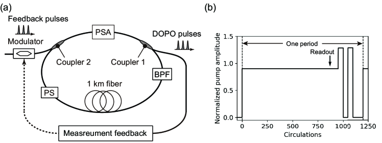
Figure 1 (a) shows the experimental setup (for details, see [13]). The CIM consists of a fiber ring cavity that contains a phase-sensitive amplifier (PSA) based on a periodically poled lithium niobate (PPLN) waveguide, two 9:1 fiber couplers, a 0.1-nm width optical bandpass filter, a piezo-based phase shifter for cavity locking, and a 1-km optical fiber. 780-nm, 1-GHz-repetition pump pulses with a -ps temporal width are launched into the PSA. When pumping starts, the PSA generates squeezed vacuum pulses through signal-idler degenerate parametric downconversion in the PPLN waveguide. The squeezed vacuum pulses circulate in the cavity while undergoing phase-sensitive amplification. Consequently, the pulse amplitude saturates after many circulations in the cavity to form 5055 DOPO pulses multiplexed in the time domain. Among the 5055 pulses, 512 (referred to as “signal pulses” hereafter) are periodically turned on and off to simulate the given Ising model many times, while the remaining pulses oscillate continuously. The DOPO pulses take only either 0 or phase relative to the pump phase as a result of the repetitive phase-sensitive amplification. By assigning 0 () as spin up (down), the DOPO phase can represent an Ising spin state. The “spin-spin interactions” among the DOPO pulses are implemented with the measurement-feedback scheme [3, 4]. In this scheme, a portion of the DOPO pulse energy is split by Coupler 1 in the ring cavity and one of the quadrature amplitudes is measured for all of the DOPO pulses by using a balanced homodyne detector. The measurement results are then analog-to-digital converted and input into a fast matrix calculation circuit realized with a field programmable gate array (FPGA). Here, the spin-spin interaction matrix for a given Ising model of size is uploaded to the FPGA in advance. The FPGA performs the multiplication of the matrix and an -element vector corresponding to the measurement results on the DOPO pulses, so that a feedback signal for each DOPO pulse is obtained in the next round trip. The feedback signal is then used to modulate the amplitude and phase of an optical pulse whose wavelength is the same as that of the DOPO pulse in the cavity, and the optical pulse is launched into the corresponding DOPO pulse through Coupler 2. Here, we denote the amplitude of the injection pulse relative to the DOPO pulses in the cavity by . We repeat the measurement-feedback procedure for each circulation in the cavity. The DOPO pulses circulate 1000 times in the cavity in accordance with the temporal schedule of the pump amplitude shown in Fig. 1 (b). The final readout of the DOPO pulse amplitudes is undertaken at the 870th circulation. With the current measurement-feedback system, we can implement all possible combinations of two-body interactions among 512 signal pulses with an 8-bit resolution.
We implemented an -spin 2D square lattice with periodic boundary conditions on the CIM. The vertical and horizontal links had the same coupling strength. Montroll et al. showed that the spontaneous magnetization of the 2D square-lattice Ising model has an exact solution at the thermodynamic limit, given by [17]
| (1) |
This equation indicates that the model exhibits a phase transition at .
In [18], it was empirically shown using one-dimensional (1D) Ising model that the effective temperature of spins represented by DOPO pulses in a CIM depends on the pump amplitude. As the pump amplitude is set closer to the oscillation threshold, the defect density decreases, implying a decrease in the effective temperature. Similar results were obtained in our numerical simulation based on quantum master equations [19], where not only the pump amplitude but also the injection amplitude altered the effective temperature of the DOPO spins. In the present experiment, the optical amplitude of the feedback pulse is supposed to be proportional to . Therefore, we ran the CIM many times for various values. is proportional to the electrical amplitude of the FPGA output signal, denoted by , which can take an integer value in the range between 0 and 127. Consequently, we obtained samples of spin sets from which we then obtained the internal energy (or sample average of the Ising energy) and magnetization values for each . As stated above, the increase in also changes the effective inverse temperature of a “spin” represented by a DOPO pulse, which means that a change in affects both and . Hereafter, we assume that and the effect of a change in is reflected in . Assuming that the energies are sampled from a canonical distribution, the energy distribution at the effective inverse temperature , , and the density of states (DOS), , can be related to with the following equation:
| (2) |
Here, is the partition function, and of the given graph can be calculated using the WL method [16]. Under this assumption, we estimate the inverse temperature by using maximum likelihood estimation. The internal energy at the estimated coincides with the theoretical value . We plotted the magnetization, entropy , and specific heat (defined later) as a function of estimated for each sample set, where denotes the experimental energy distribution. Regarding the magnetization, we used the root mean square (RMS) of .
We implemented a 2D square-lattice Ising model with . The periodic boundary conditions were implemented by taking advantage of the flexible spin-spin interaction enabled by the measurement feedback. We embedded four graphs together with a 32-node bipartite graph that was used as a “monitor graph” to the signal pulses. These graphs were multiplied with a 432 432 random permutation and spin flip matrix so that the temporal positions and the signs of the spins were randomized to avoid forming ferromagnetic states due to experimental imperfections such as reflections of light inside the fiber cavity.
The CIM performed 256 computations in a single batch of measurements, which yielded 1048 spin sets for the 100-node 2D Ising model. In order to extract results obtained when the CIM stably operated, we eliminated results when the Ising energy of the monitor graph did not reach the ground state. We then used the energies of the remaining results in the batch to estimate . We set 22 values of the amplitude of the FPGA output signal , ranging from 0 to 125, and obtained ten batches of results for each value. We repeated this procedure four times, which means that we accumulated 40,960 spin sets for each value of . On average, 8% of the spin sets passed the filtering by the monitor graph.
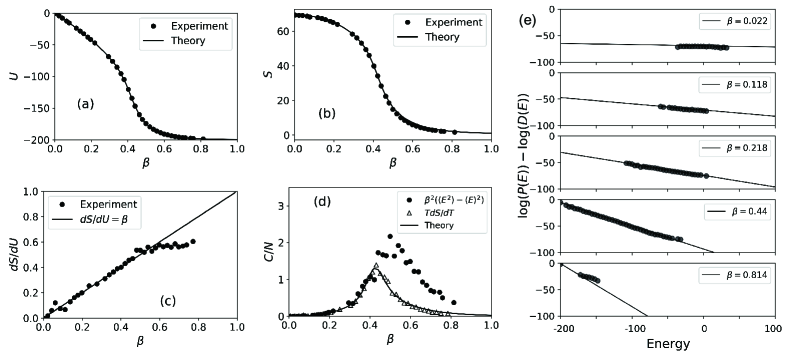
Figure 2 (a) shows the internal energy as a function of the estimated , which fits the theoretical curve as a natural result of the maximum likelihood estimation. The experimental entropy as a function of the estimated is shown by the circles in Fig. 2 (b). The experimental data clearly fits the theoretical curve, suggesting that not only the average energy but also the energy distribution agree with the theory based on the canonical distribution assumption. Using the and relationships, we plotted the curve, and obtained the thermodynamic inverse temperature defined as . The relationship between the obtained and estimated is shown in Fig. 2 (c), which indicates that the estimated temperatures were close to the thermodynamic temperature for up to .
The experimental and theoretical specific heats are shown in Fig. 2 (d). The circles show the experimental specific heat derived from the Ising energies and the statistical-mechanical relationship , and the triangles denote another set of experimental values obtained from the estimated entropy (Fig. 2 (b)) and the thermodynamic relationship . The circles form a clear peak structure that is a characteristic of the theoretical specific heat as a function of temperature, but at a clearly larger . Since is proportional to the variance of the energy, the experimental instability enhanced at around the transition point may have caused the discrepancy from the theory. On the other hand, (the triangles) fits the theoretical curve very well, which suggests that the spin sets produced by the CIM satisfy the thermodynamic relationship.
Using the estimated , we plotted as a function of energy, which should be a linear function with slope . The results are shown in Fig. 2 (e); the experimentally observed distributions fit the theoretical line for the canonical distribution at a around the theoretical transition point () or smaller. In contrast, there is a clear discrepancy from the theoretical line at a relatively larger . This suggests that the effective temperatures obtained in our experiment are close to the value obtained by statistical mechanics under the canonical distribution assumption, except at temperatures significantly below the transition temperature. Note that this tendency resembles the one observed in the curve shown in Fig. 2 (c), where the thermodynamic inverse temperatures are smaller than the effective for . The validity of the estimated effective temperatures was quantified by the Kullback-Leibler divergence (see Supplemental Material [20]). We should emphasize here that the present diffusive system satisfies the canonical distribution assumption throughout most of the temperature region. The experimentally estimated temperature, thermodynamic temperature, and statistical-mechanics temperature under the canonical distribution assumption are in very good agreement, except at very low temperatures.
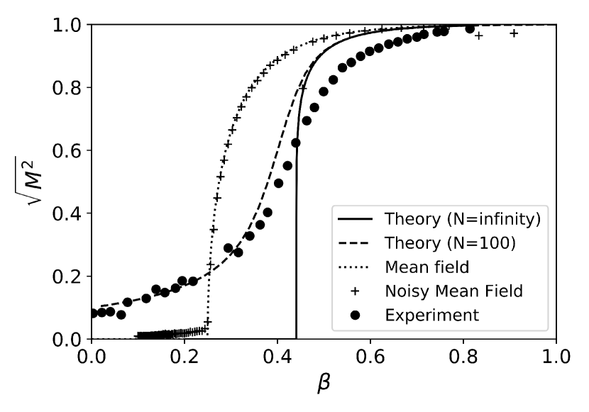
Next, we plotted the RMS magnetization as a function of the effective . As is apparent from Fig. 3, the experimental result exhibits a clear phase-transition-like behavior in the finite-sized system with a critical temperature at . In addition, the RMS magnetization curve obtained by the CIM is closer than the MF one (dotted line) to the theoretical curve of in the thermodynamic limit (solid line) and the theoretical curve of for the case of calculated using the DOS obtained by the WL method (dashed line).
Finally, we performed a numerical simulation using an algorithm based on MF dynamics (noisy MF annealing) [15]. Here, we set the standard deviation of the Gaussian noise and the amplitude splitting parameter to the same values in [15] (both 0.15). As expected, the results (the plots in Fig. 3) were close to the MF solution. These observations indicate that the CIM in its present operational condition well simulates the thermodynamic properties of the Ising model, which are presumably hard to reproduce with the MF approach.
It is not yet clear what caused the discrepancy between the estimated temperatures and the thermodynamic temperatures at in Fig.2 (c). A possible origin of the discrepancy is “mode selection”, which was observed in our numerical simulation of the CIM [19]. In this phenomenon, some instances of the Ising model show a tendency that certain spin configurations are more likely to appear when the pump amplitude is relatively large. Such “selected modes” are visible in the bottom panel of Fig. 2 (e), where the observed energies are discontinuous and do not fit the line that corresponds to the canonical distribution. The formation of such modes may have prevented the thermodynamic inverse temperature from increasing above . Also, the mode-selection phenomenon may have caused a deviation from the canonical distribution in the low-temperature region, which in turn may have caused the deviation in the experimental specific heat from theory in Fig. 2 (d). A similar phenomenon is so-called “freeze out”, which was theoretically discussed in [21] and experimentally observed in [12]. In this phenomenon, when the pump amplitude is sufficiently larger than the oscillation threshold, the DOPO dynamics stop before reaching the ground or low-energy states. We suspect that this effect may be the origin of the mode selection. Further theoretical and experimental investigation are needed on these issues.
Recently, several studies on phase transitions simulated on optical Ising machines have been reported [22, 23]. We should point out that the results of these papers matched those of the MF models, whereas our results are in a clear distinction from what is predicted by MF theory. Another fact that differentiates our work from the literature is that we examined the validity of the effective temperature by observing not only the spontaneous magnetization but also other physical quantities, namely the entropy and the specific heat, and found that the CIM well simulates a thermodynamic system except at very low temperature. MF theory, on the other hand, violates thermodynamic relationships except for a few particular models.
In summary, we simulated the phase transition of a 2D square-lattice Ising model on the CIM. We confirmed that for relatively small , the CIM provides a consistent description of Ising spins in thermal equilibrium from multiple viewpoints, namely thermodynamics, statistical mechanics, and statistical inference. With the obtained thermodynamic quantities, we observed phase-transition-like behavior in a finite-sized system with a transition temperature close to the theoretical value. These results indicate that the CIM is an optical realization of a thermodynamic spin system where all the spins can be independently accessed. We may utilize these characteristics for information processing tasks such as Boltzmann sampling and fast simulation of magnetic systems.
H. T. and Y. Yamada contributed equally to this work.
References
- [1] N. Mohseni, P. L. McMahon, and T. Byrnes, “Ising machines: hardware solvers for combinatorial optimization problems,” Nat. Rev. Phys. 4, 363 (2022).
- [2] A. Marandi, Z. Wang, K. Takata, R. L. Byer, and Y. Yamamoto, “Network of time-multiplexed optical parametric oscillators as a coherent Ising machine,” Nat. Photon. 8, 937-942 (2014).
- [3] T. Inagaki, Y. Haribara, K. Igarashi, T. Sonobe, S. Tamate, T. Honjo, A. Marandi, P. L. McMahon, T. Umeki, K. Enbutsu, O. Tadanaga, H. Takenouchi, K. Aihara, K. Kawarabayashi, K. Inoue, S. Utsunomiya, and H. Takesue, “A coherent Ising machine for 2000-node optimization problems,” Science 354, 603-606 (2016).
- [4] P. L. McMahon, A. Marandi, Y. Haribara, R. Hamerly, C. Langrock, S. Tamate, T. Inagaki, H. Takesue, S. Utsunomiya, K. Aihara, R. L. Byer, M. M. Fejer, H. Mabuchi, and Y. Yamamoto, “A fully-programmable 100-spin coherent Ising machine with all-to-all connections,” Science 354, 614-617 (2016).
- [5] R. Hamerly, T. Inagaki, P. L. McMahon, D. Venturelli, A. Marandi, T. Onodera, E. Ng, C. Langrock, K. Inaba, T. Honjo, K. Enbutsu, T. Umeki, R. Kasahara, S. Utsunomiya, S. Kako, K. Kawarabayashi, R. L. Byer, M. M. Fejer, H. Mabuchi, D. Englund, E. Rieffel, H. Takesue and Y. Yamamoto, “Experimental investigation of performance differences between Coherent Ising Machines and a quantum annealer,” Sci. Adv. 5, eaau0823 (2019).
- [6] T. Honjo, T. Sonobe, K. Inaba, T. Inagaki, T. Ikuta, Y. Yamada, T. Kazama, K. Enbutsu, T. Umeki, R. Kasahara, K. Kawarabayashi, and H. Takesue, “100,000-spin coherent Ising machine,” Sci. Adv. 7, eabh0952 (2021).
- [7] D. Pierangeli, G. Marcucci, and C. Conti, “Large-scale photonic Ising machine by spatial light modulation,” Phys. Rev. Lett. 122, 213902 (2019).
- [8] F. Böhm, G. Verschaffelt, and G. Van der Sande, “A poor man’s coherent Ising machine based on opto-electronic feedback systems for solving optimization problems, “ Nat. Commun. 10, 3538 (2019).
- [9] M. Babaeian, D. T. Nguyen, V. Demir, M. Akbulut, P.-A. Blanche, Y. Kaneda, S. Guha, M. A. Neifeld and N. Peyghambarian, “A single shot coherent Ising machine based on a network of injection-locked multicore fiber lasers,” Nat. Commun. 10, 3516 (2019).
- [10] Y. Okawachi, M. Yu, J. K. Jang, X. Ji, Y. Zhao, B. Y. Kim, M. Lipson, and A. L. Gaeta, “Demonstration of chip-based coupled degenerate optical parametric oscillators for realizing a nanophotonic spin-glass,” Nat. Commun. 11, 4119 (2020).
- [11] T. Inagaki, K. Inaba, T. Leleu, T. Honjo, T. Ikuta, K. Enbutsu, T. Umeki, R. Kasahara, K. Aihara, and H. Takesue, “Collective and synchronous dynamics of photonic spiking neurons,” Nat. Commun. 12, 2325 (2021)
- [12] F. Böhm, T. Inagaki, K. Inaba, T. Honjo, K. Enbutsu, T. Umeki, R. Kasahara, and H. Takesue, “Understanding dynamics of coherent Ising machines through simulation of large-scale 2D Ising models,” Nat. Commun. 9, 5020 (2018).
- [13] H. Takesue, K. Inaba, T. Inagaki, T. Ikuta, Y. Yamada, T. Honjo, T. Kazama, K. Enbutsu, T. Umeki, R. Kasahara, “Simulating Ising spins in external magnetic fields with a network of degenerate optical parametric oscillators,” Phys. Rev. Appl. 13, 054059 (2020).
- [14] L. Onsager, “Crystal statistics. I. A two-dimensional model with an order-disorder transition,” Phys. Rev. 65, 117 (1944).
- [15] A. D. King, W. Bernoudy, J. King, A. J. Berkley, T. Lanting, “Emulating the coherent Ising machine with a mean-field algorithm,” arXiv:1806.08422 (2018).
- [16] F. Wang and D. P. Landau, “Efficient, multiple-range random walk algorithm to calculate the density of states,” Phys. Rev. Lett. 86, 2050 (2001).
- [17] E. W. Montroll, R. B. Potts, and J. C. Ward, “Correlations and spontaneous magnetization of the two-dimensional Ising model,” J. Math. Phys. 4, 308 (1963)
- [18] T. Inagaki, K. Inaba, R. Hamerly, K. Inoue, Y. Yamamoto, and H. Takesue, “Large-scale Ising spin network based on degenerate optical parametric oscillators,” Nat. Photon. 10, 415-419 (2016).
- [19] Y. Yamada and K. Inaba, “Dissipative quantum dynamics in coherent Ising machine with measurement-feedback spin-spin couplings,” Adiabadic Quantum Computing (AQC) 2021, Day 1, Poster B2 (2021).
- [20] See Supplemental Material at http://xxxxx for Kullback-Leibler divergence of the experimentally obtained energy distributions against the canonical distribution obtained using the WL method, the effect of DOPO amplitude heterogeneity, and difference from previous studies on CIM, and Refs. [24, 25].
- [21] R. Hamerly, K. Inaba, T. Inagaki, H. Takesue, Y. Yamamoto, and H. Mabuchi, “Topological defect formation in 1D and 2D spin chains realized by network of optical parametric oscillators,” Int. J. Mod. Phys. B 30, 1630014 (2016).
- [22] Y. Fang, J. Huang, and Z. Ruan, “Experimental observation of phase transition in spatial Ising machine,” Phys. Rev. Lett. 127, 043902 (2021).
- [23] S. Kumar, Z. Li, T. Bu, C. Qu, Y. Huang, “Observation of distinct phase transitions in a nonlinear optical Ising machine,” Commun. Phys. 6, 31 (2023).
- [24] Y. Yamamoto, K. Aihara, T. Leleu, K. Kawarabayashi, S. Kako, M. Fejer, K. Inoue, and H. Takesue, “Coherent Ising machines-optical neural networks operating at the quantum limit,” npj Quantum Information 3, 49 (2017).
- [25] Y. Takeda, S. Tamate, Y. Yamamoto, H. Takesue, T. Inagaki, and S. Utsunomiya, “Bolzmann sampling for an XY model using a non-degenerate optical parametric oscillator network,” Quantum Sci. Technol. 3, 014004 (2018).