Simplifying Subgraph Representation Learning
for Scalable Link Prediction

Abstract.

Link prediction on graphs is a fundamental problem, addressing the task of predicting potential connections between entities in a network, enabling the identification of missing or future relationships. Its applications span various domains, including social networks, recommendation systems, and biological networks, where predicting links can enhance our understanding of network structure and facilitate more effective information dissemination or resource allocation. Subgraph representation learning approaches (SGRLs), by transforming link prediction to graph classification on the subgraphs around the links, have achieved state-of-the-art performance in link prediction. However, SGRLs are computationally expensive and not scalable to large-scale graphs due to expensive subgraph-level operations. To unlock the scalability of SGRLs, we propose a new class of SGRLs, that we call Scalable Simplified SGRL (S3GRL). Aimed at faster training and inference, S3GRL simplifies the message passing and aggregation operations in each link’s subgraph. S3GRL, as a scalability framework, accommodates various subgraph sampling strategies and diffusion operators to emulate computationally expensive SGRLs. We propose multiple instances of S3GRL and empirically study them on small to large-scale graphs. Our extensive experiments demonstrate that the proposed S3GRL models scale up SGRLs without significant performance compromise (even with considerable gains in some cases), while offering substantially lower computational footprints (e.g., multi-fold inference and training speedup).

1. Introduction

Graphs are ubiquitous in representing relationships between interacting entities in a variety of contexts, ranging from social networks (Chen et al., 2020) to polypharmacy (Zitnik et al., 2018). One of the main tasks on graphs is link prediction (Liben-Nowell and Kleinberg, 2003), which involves predicting future or missing relationships between pairs of entities, given the graph structure. Link prediction plays a fundamental role in impactful areas, including molecular interaction predictions (Huang et al., 2020), recommender systems (Ying et al., 2018), and protein-protein interaction predictions (Zhong et al., 2022).

The early solutions to link prediction relied on hand-crafted, parameter-free heuristics based on the proximity of the source-target nodes (Page et al., 1999; Adamic and Adar, 2003). However, these methods require extensive domain knowledge for effective implementation. Recently, the success of graph neural networks (GNNs) in learning latent representations of nodes (Kipf and Welling, 2017) has led to their application in link prediction, through aggregating the source-target nodes’ representations as a link representation (Kipf and Welling, 2016; Pan et al., 2018). However, as GNNs learn a pair of nodes’ representations independent of their relative positions to each other, aggregating independent node representations results in poor link representations (Zhang et al., 2021). To circumvent this, the state-of-the-art subgraph representation learning approaches (SGRLs) (Zhang and Chen, 2018) learn enclosing subgraphs of pairs of source-target nodes, while augmenting node features with structural features. By doing so, the link prediction problem is cast as a binary graph classification on the enclosing subgraph about a link.

The core issue hampering the deployment of GNNs and SGRLs is their high computational demands on large-scale graphs (e.g., OGB datasets (Hu et al., 2020, 2021)). Many approaches have been proposed for GNNs to relieve this bottleneck, ranging from sampling (Chen et al., 2018; Zeng et al., 2020) to simplification (Wu et al., 2019) techniques. However, these techniques fail to be applied directly in SGRL models, where the issue is even more adverse due to subgraph extractions pertaining to each link. Although recent work has focused on tackling SGRL scalability by sampling (Yin et al., 2022; Louis et al., 2022) or sketching (Chamberlain et al., 2023) approaches, little attention is given to simplification techniques. We focus on improving the scalability in SGRLs by simplifying the underlying training mechanism.

Inspired by the simplification techniques in GNNs such as SGCN (Wu et al., 2019) and SIGN (Frasca et al., 2020), we propose Scalable Simplified SGRL (S3GRL) framework, which extends the simplification techniques to SGRLs. Our S3GRL is flexible in emulating many SGRLs by offering choices of subgraph sampling and diffusion operators, producing different-sized convolutional filters for each link’s subgraph. Our S3GRL benefits from precomputing the subgraph diffusion operators, leading to an overall reduction in runtimes while offering a multi-fold scale-up over existing SGRLs in training/inference times. We propose and empirically study multiple instances of our S3GRL framework. Our extensive experiments show substantial speedups in S3GRL models over state-of-the-art SGRLs while maintaining and sometimes surpassing their efficacies. The key contributions are summarized as follows:

• We proposed our S3GRL framework to extend simplification methods introduced in graph neural networks to the context of subgraph representation learning.

• Focusing on the link prediction problem, we introduce multiple instantiations of our S3GRL to showcase the flexibility, robustness, and scalability of our framework. We theoretically analyze the inference time complexity, preprocessing time complexity, and storage requirement of our methods and contrasted them with their competitive counterparts.

• We empirically study and evaluate the performance of our S3GRL instances on 14 small-to-large graph datasets under various evaluation criteria. Our empirical studies and analyses include deep comparisons of our methods against 16 competitive baselines widely utilized in link prediction studies.

• Our empirical results confirm the efficacy improvements of our S3GRL methods over others while offering multi-fold speed-up in training and inference.

• Our results also demonstrate a multi-fold reduction in storage requirements: The S3GRL preprocessed datasets are multiple magnitudes smaller than those of other SGRLs (e.g., SEAL (Zhang and Chen, 2018)).

• We share our findings and framework as an open-source framework, enabling other researchers to devise and test their own S3GRL instances, thereby advancing link prediction research.

2. Related Work

Graph representation learning (GRL) (Hamilton, 2020) has numerous applications in drug discovery (Xiong et al., 2019), knowledge graph completion (Zhang et al., 2020), and recommender systems (Ying et al., 2018). The key downstream tasks in GRL are node classification (Hamilton et al., 2017), link prediction (Zhang and Chen, 2018) and graph classification (Zhang et al., 2018). The early work in GRL, shallow encoders (Perozzi et al., 2014; Grover and Leskovec, 2016), learns dense latent node representations by taking multiple random walks rooted at each node. However, shallow encoders were incapable of consuming node features and being applied in the inductive settings. This shortcoming led to growing interest in Message Passing Graph Neural Networks (MPGNNs) (Bruna et al., 2014; Defferrard et al., 2016) such as Graph Convolutional Networks (GCN) (Kipf and Welling, 2017). In MPGNNs, node feature representations are iteratively updated by first aggregating neighborhood features and then updating them through non-linear transformations. MPGNNs differ in formulations of aggregation and update functions (Hamilton, 2020).

Link prediction is a fundamental problem on graphs, where the objective is to compute the likelihood of the presence of a link between a pair of nodes (e.g., users in a social network) (Liben-Nowell and Kleinberg, 2003). Network heuristics such as Common Neighbors or Katz Index (Katz, 1953) were the first solutions for link prediction. However, these predefined heuristics fail to generalize well on different graphs. To address this, MPGNNs have been used to learn representations of node pairs independently, then aggregate the representations for link probability prediction (Kipf and Welling, 2016; Mavromatis and Karypis, 2021). However, this class of MPGNN solutions falls short in capturing graph automorphism and different structural roles of nodes in forming links (Zhang et al., 2021). SEAL (Zhang and Chen, 2018) successfully overcomes this limitation by casting the link prediction problem as a binary graph classification on the enclosing subgraph about a link, and adding structural labels to node features. This led to the emergence of subgraph representation learning approaches (SGRLs) (Zhang and Chen, 2018; Li et al., 2020), which offer state-of-the-art results on the link prediction task. However, a common theme impeding the practicality and deployment of SGRLs is its lack of scalability to large-scale graphs.

Recently, a new research direction has emerged in GNNs on scalable training and inference techniques, which mainly focuses on node classification tasks. A common practice is to use different sampling techniques—such as node sampling (Hamilton et al., 2017), layer-wise sampling (Zou et al., 2019), and graph sampling (Zeng et al., 2020)—to subsample the training data to reduce computation. Other approaches utilize simplification techniques, such as removing intermediate non-linearities (Wu et al., 2019; Frasca et al., 2020), to speed up the training and inference. These approaches have been shown to fasten learning of MPGNNs (at the global level) for node and graph classification tasks, and even for link prediction (Pho and Mantzaris, 2022); however, they are not directly applicable to SGRLs which exhibit superior performance for link prediction. In this work, we take the scalability-by-simplification approach for SGRLs (rather than for MPGNNs) by introducing Scalable Simplified SGRL (S3GRL). Allowing diverse definitions of subgraphs and subgraph-level diffusion operators for SGRLs, S3GRL emulates SGRLs in generalization while speeding them up.

There is a growing interest in the scalability of SGRLs (Yin et al., 2022; Louis et al., 2022; Chamberlain et al., 2023), with a main emphasis on the sampling approaches. SUREL (Yin et al., 2022), by deploying random walks with restart, approximates subgraph structures; however, it does not use GNNs for link prediction. ScaLed (Louis et al., 2022) uses similar sampling techniques of SUREL, but to sparsify subgraphs in SGRLs for better scalability. ELPH/BUDDY (Chamberlain et al., 2023) uses subgraph sketches as messages in MPGNNs but does not learn link representations explicitly at a subgraph level. Most recently, sampling techniques have improved scalability in subgraph classification tasks (Jacob et al., 2023). Our work complements this body of research. Our framework can be combined with (or host) these methods for better scalability (see our experiments for an example).

3. Preliminaries

Consider a graph $G=(V,E)$, where $V=\{1,\dots,n\}$ is the set of nodes (e.g., individuals, proteins), $E\subseteq V\times V$ represents their relationships (e.g., friendship or protein-to-protein interactions). We also let $\mathbf{A}\in\mathbb{R}^{n\times n}$ represent the adjacency matrix of $G$, where $A_{uv}\neq 0$ if and only if $(u,v)\in E$. We further assume each node possesses a $d$-dimensional feature vector (e.g., user’s profile, features of proteins, etc.) stored as a row in feature matrix $\mathbf{X}\in\mathbb{R}^{n\times d}$.

Link Prediction. The goal is to infer the presence or absence of an edge between target nodes $T=\{u,v\}$ given the observed matrices $\mathbf{A}$ and $\mathbf{X}$. The learning problem is to find a likelihood function $f$ such that it assigns a higher likelihood to those target nodes with a missing link. The likelihood function can be formulated by various neural network architectures (e.g., MLP (Guo et al., 2022) or GNNs (Davidson et al., 2018)).

GNNs. Graph Neural Networks (GNNs) typically take as input $\mathbf{A}$ and $\mathbf{X}$, apply $L$ layers of convolution-like operations, and output $\mathbf{Z}\in\mathbb{R}^{n\times d^{\prime}}$, containing $d^{\prime}$-dimensional representation for each node as a row. For example, the $l^{th}$-layer output of Graph Convolution Network (GCN) (Kipf and Welling, 2017) is given by

(1) $$\mathbf{H}^{(l)}=\sigma\left(\hat{\mathbf{A}}\mathbf{H}^{(l-1)}\mathbf{W}^{(l-1)}\right),$$

where normalized adjacency matrix $\hat{\mathbf{A}}=\tilde{\mathbf{D}}^{-\frac{1}{2}}\tilde{\mathbf{A}}\tilde{\mathbf{D}}^{-\frac{1}{2}}$, $\tilde{\mathbf{A}}=\mathbf{A}+\mathbf{I}$, $\tilde{\mathbf{D}}$ is the diagonal matrix with $\tilde{D}_{ii}=\sum_{j}\tilde{A}_{ij}$, and $\sigma$ is a non-linearity function (e.g., ReLU). Here, $\mathbf{H}^{(0)}=\mathbf{X}$ and $\mathbf{W}^{(l)}$ is the $l^{th}$ layer’s learnable weight matrix. After $L$ stacked layers of Eq. 1, GCN outputs nodal-representation matrix $\mathbf{Z}=\mathbf{H}^{(L)}$. For any target nodes $T=\{u,v\}$, one can compute its joint representation:

(2) $$\mathbf{q}_{uv}=\operatorname{pool}\left(\mathbf{z}_{u},\mathbf{z}_{v}\right),$$

where $\mathbf{z}_{u}$, $\mathbf{z}_{v}$ are $u$’s and $v$’s learned representations in $\mathbf{Z}$, and $\operatorname{pool}$ is a pooling/readout operation (e.g., Hadamard product or concatenation) to aggregate the pairs’ representations. Then, the link probability $p(u,v)$ for the target is given by $p(u,v)=\Omega(\mathbf{q}_{uv})$, where $\Omega$ is a learnable non-linear function (e.g., MLP) transforming the target embedding $\mathbf{q}_{uv}$ into a link probability.

Figure 1. Our S3GRL framework: In the preprocessing phase (shown by the shaded blue arrow), first multiple subgraphs are extracted around the target nodes $u$ and $v$ (shaded in blue) by various sampling strategies. Diffusion matrices are then created from extracted subgraph adjacency matrices by predefined diffusion operators (e.g., powers of subgraphs in this figure). Each diffusion process involves the application of the subgraph diffusion matrix on its nodal features to create the matrix $\mathbf{Z}^{(i)}_{uv}$. The operator-level node representations of selected nodes (with a red border in raw data) are then aggregated for all subgraphs to form the joint $\mathbf{Z}_{uv}$ matrix. The selected nodes in this example are the target nodes $\{u,v\}$, and their common neighbor $d$. In the learning phase (as shown by the shaded red arrow), the joint matrix $\mathbf{Z}_{uv}$ undergoes dimensionality reduction followed by pooling using center pooling (highlighted by blue-border box) and common neighbor pooling (highlighted by purple-border box). Finally, the target representation $\textbf{q}_{uv}$ is transformed by an MLP to a link probability $P_{uv}$.

SGRLs. Subgraph representation learning approaches (SGRLs) (Zhang and Chen, 2017, 2018; Zhang et al., 2021; Yin et al., 2022; Louis et al., 2022) treat link prediction as a binary graph classification problem on enclosing subgraph $G_{uv}=(V_{uv}\subseteq V,E_{uv}\subseteq E)$ around a target $\{u,v\}$. SGRLs aim to classify if the enclosing subgraph $G_{uv}$ is closed or open (i.e., the link exists or not). For each $G_{uv}$, SGRLs produce its nodal-representation matrix $\mathbf{Z}_{uv}$ using the stack of graph convolution operators (see Eq. 1). Then, similar to Eq. 2, the nodal representations would be converted to link probabilities, with the distinction that the pooling function is graph pooling (e.g., SortPooling (Zhang et al., 2018)), operating over all node’s representations (not just those of targets) to produce the fixed-size representation of the subgraph. To improve the expressiveness of GNNs on subgraphs, SGRLs augment node features with some structural features determined by the targets’ positions in the subgraph. These augmented features are known as node labels (Zhang et al., 2021). Node labeling techniques fall into zero-one or geodesic distance-based schemes (Huang et al., 2022). We refer to $\mathbf{X}_{uv}$ as the matrix containing both the initial node features and labels generated by a valid labeling scheme (Zhang et al., 2021). The expressiveness power of SGRLs comes with high computational costs due to subgraph extractions, node labeling, and independent operations on overlapping large subgraphs. This computational overhead is exaggerated in denser graphs and deeper subgraphs due to the exponential growth of subgraph size.

SGCN and SIGN. To improve the scalability of GNNs for node classification tasks, several attempts are made to simplify GNNs by removing their intermediate nonlinearities, thus making them shallower, easier to train, and scalable. Simplified GCN (SGCN) (Wu et al., 2019) has removed all intermediate non-linearities in L-layer GCNs, to predict class label probabilities $\mathbf{Y}$ for all nodes by $\mathbf{Y}=\xi(\hat{\mathbf{A}}^{L}\mathbf{X}\mathbf{W})$, where $\xi$ is softmax or logistic function, and $\mathbf{W}$ is the only learnable weight matrix. The term $\hat{\mathbf{A}}^{L}\mathbf{X}$ can be precomputed once before training. Benefiting from this precomputation and a shallower architecture, SGCN improves scalability. SIGN has extended SGCN to be more expressive yet scalable for node classification tasks. Its crux is to deploy a set of linear diffusion matrices $\mathbf{M}^{(1)},\dots,\mathbf{M}^{(r)}$ that can be applied to node-feature matrix $\mathbf{X}$. The class probabilities $\mathbf{Y}$ are computed by $\mathbf{Y}=\xi(\mathbf{Z}\mathbf{W}^{\prime})$, where

(3) $$\mathbf{Z}=\sigma\left(\bigoplus_{i=0}^{r}\mathbf{M}^{(i)}\mathbf{X}\mathbf{W}_{i}\right).$$

Here, $\xi$ and $\sigma$ are non-linearities, $\mathbf{W}_{i}$ is the learnable weight matrix for diffusion operator $\mathbf{M}^{(i)}$, $\bigoplus$ is a concatenation operation, and $\mathbf{W}^{\prime}$ is the learnable weight matrix for transforming node representations to class probabilities. Letting $\mathbf{I}$ be the identity matrix, $\mathbf{M}^{(0)}=\mathbf{I}$ in Eq. 3 allows the node features to contribute directly (independent of graph structure) into the node representation and consequently to the class probabilities. The $\mathbf{M}^{(i)}$ operator captures different heuristics in the graph. As with SGCN, the terms $\mathbf{M}^{(i)}\mathbf{X}$ in SIGN can be once precomputed before training. These precomputations and the shallow architecture of SIGN lead to substantial speedup during training and inference with limited compromise on node classification efficacy. Motivated by these efficiencies, our S3GRL framework extends SIGN for link prediction on subgraphs while addressing the computational bottleneck of SGRLs.

4. Scalable Simplified SGRL (S3GRL)

We propose Scalable Simplified SGRL (S3GRL), which benefits from the expressiveness power of SGRLs while offering the simplicity and scalability of SIGN and SGCN for link prediction. Our framework leads to a multi-fold speedup in both training and inference of SGRL methods while maintaining or boosting their state-of-the-art performance (see experiments below).

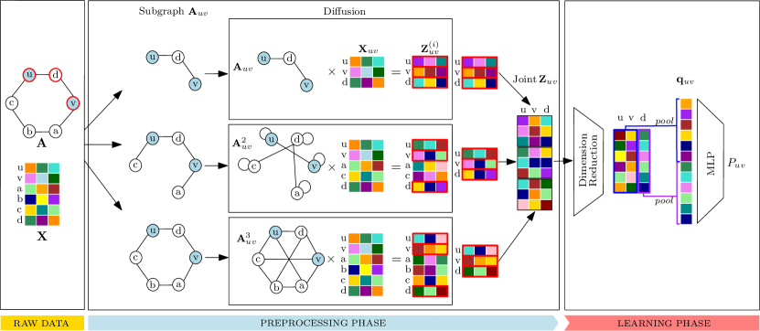
Our S3GRL framework consists of two key components: (i) Subgraph sampling strategy $\Psi(G,T)$ takes as an input the graph $G$ and target pairs $T=\{u,v\}$ and outputs the adjacency matrix $\mathbf{A}_{uv}$ of the enclosing subgraphs $G_{uv}$ around the targets. The subgraph sampling strategy $\Psi$ can capture various subgraph definitions such as $h$-hop enclosing subgraphs (Zhang and Chen, 2018)), random-walk-sampled subgraphs (Yin et al., 2022; Louis et al., 2022), and heuristic-based subgraphs (Zeng et al., 2021); (ii) Diffusion operator $\Phi(\mathbf{A}_{uv})$ takes the subgraph adjacency matrix $\mathbf{A}_{uv}$ and outputs its diffusion matrix $\mathbf{M}_{uv}$. A different class of diffusion operators are available: adjacency/Laplacian operators to capture connectivity, triangle/motif-based operators (Granovetter, 1983) to capture inherent community structure, personalized pagerank-based (PPR) operators (Gasteiger et al., 2019) to identify important connections. Each of these operators and their powers can constitute the different diffusion operators in S3GRL.

In our S3GRL framework, each model is characterized by the sampling-operator set $\mathcal{S}=\{(\Psi_{i},\Phi_{i})\}_{i=0}^{r}$, where $\Psi_{i}$ and $\Phi_{i}$ are the $i^{th}$ subgraph sampling strategy and diffusion operator, respectively. For a graph $G$, target pair $T=\{u,v\}$, and sampling-operator pair $(\Psi_{i},\Phi_{i})$, one can find $T$’s sampled subgraph $\mathbf{A}^{(i)}_{uv}=\Psi_{i}(G,T)$ and its corresponding diffusion matrix $\mathbf{M}^{(i)}_{uv}=\Phi_{i}(\mathbf{A}^{(i)}_{uv})$. For instance, one can define $\Psi_{i}$ to sample the random-walk-induced subgraph $\mathbf{A}_{uv}^{(i)}$ rooted at $\{u,v\}$ in $G$. Then, $\Phi_{i}$ can compute the $l$-th power of $\mathbf{A}_{uv}^{(i)}$, to count the number of $l$-length walks on the subgraph. S3GRL computes the operator-level node representations of the selected subgraph $\mathbf{A}^{(i)}_{uv}$ by

(4) $$\mathbf{Z}^{(i)}_{uv}=\mathbf{M}^{(i)}_{uv}\mathbf{X}^{(i)}_{uv}.$$

Here, $\mathbf{X}^{(i)}_{uv}$ is the node feature matrix for nodes in the selected subgraph $\mathbf{A}^{(i)}_{uv}$ for the sampling-operator pair $(\Psi_{i},\Phi_{i})$. Eq. 4 can be viewed as feature smoothing where the diffusion matrix $\mathbf{M}^{(i)}_{uv}$ is applied over node features $\mathbf{X}^{(i)}_{uv}$. S3GRL then concatenates the operator-level nodal-representation matrix $\mathbf{Z}^{(i)}_{uv}$ of all sampling-operator pairs to form the joint nodal-representation matrix:

(5) $$\mathbf{Z}_{uv}=\bigoplus_{i=0}^{r}\mathbf{Z}^{(i)}_{uv}$$

The concatenation between nodal-representation matrices with dimensionality mismatch should be done with care: the corresponding rows (belonging to the same node) should be inline, where missing rows are filled with zeros (analogous to zero-padding for graph pooling). The joint nodal-representation matrix $\mathbf{Z}_{uv}$ goes through a non-linear feature transformation (for dimensionality reduction) by learnable weight matrix $\mathbf{W}$ and non-linearity $\sigma$. This transformed matrix is then further downsampled by the graph pooling $\operatorname{pool}$ to form the target’s representation:

(6) $$\mathbf{q}_{uv}=\operatorname{pool}\left(\sigma\left(\mathbf{Z}_{uv}\mathbf{W}\right)\right),$$

from which the link probability is computed by

(7) $$P_{uv}=\Omega(\mathbf{q}_{uv}),$$

with $\Omega$ being a learnable non-linear function (e.g., MLP) to convert the target representation $\mathbf{q}_{uv}$ into a link probability.

Our S3GRL exhibits substantial speedup in inference and training through precomputing $\mathbf{Z}_{uv}$ in comparison to more computationally-intensive SGRLs (Li et al., 2020; Pan et al., 2022), designed based on multi-layered GCN or DGCNN (Zhang et al., 2018) (see our experiments for details). Note that only Equations 6 and 7 are utilized in training and inference in S3GRL (see also Figure 1). Apart from this computational speedup, S3GRL offers other advantages analogous to other prominent GNNs:

Disentanglement of Data and Model. The composition of subgraph sampling strategy $\Psi$ and diffusion operator $\Phi$ facilitates the disentanglement (or decoupling) of data (i.e., subgraph) and model (i.e., diffusion operator). This disentanglement resembles shaDow-GNN (Zeng et al., 2021), in which the depth of GNNs (i.e., its number of layers) is decoupled from the depth of enclosing subgraphs. Similarly, in S3GRL, one can explore high-order diffusion operators (e.g., adjacency matrix to a high power) in constrained enclosing subgraphs (e.g., ego network of the target pair). This combination simulates multiple message-passing updates between the nodes in the local subgraph, thus achieving local oversmoothing (Zeng et al., 2021) and ensuring the final subgraph representation possesses information from all the nodes in the local subgraph.

Multi-View Representation. Our S3GRL framework via the sampling-operator pairs provides multiple views of the enclosing neighborhood of each target pair. This capability allows hosting models analogous to multi-view (Abu-El-Haija et al., 2020; Cai and Ji, 2020) models.

5. S3GRL Instances and Computational Complexities

We introduce two instances of S3GRL, differentiating in the choice of sampling-operator pairs, which we call Powers of Subgraphs (PoS) and Subgraphs of Powers (SoP). We then present our graph pooling methods for these two instances. Finally, we deep dive into computational time complexity analyses of these variants and compare them with their competitive counterparts SEAL (Zhang and Chen, 2018).

5.1. Powers of Subgraphs (PoS)

This instance intends to mimic a group of SGRLs with various model depths on a fixed-sized enclosing subgraph while boosting scalability and generalization (e.g., SEAL (Zhang and Chen, 2018)). The sampling-operator set $\mathcal{S}=\{(\Psi_{i},\Phi_{i})\}_{i=0}^{r}$ is defined as follows: (i) the sampling strategy $\Psi_{i}(G,T)$ for any $i$ is constant and returns the adjacency matrix $\mathbf{A}_{uv}$ of the $h$-hop enclosing subgraph $G_{uv}^{h}$ about target $T=\{u,v\}$. The subgraph $G_{uv}^{h}$ is a node-induced subgraph of $G$ with the node set $V^{h}_{uv}=\{j|d(j,u)\leq h\ or\ d(j,v)\leq h\}$, including the nodes with the geodesic distance of at most $h$ from either of the target pairs (Zhang and Chen, 2018); (ii) the $i$-th diffusion operator $\Phi_{i}(\mathbf{A})=\mathbf{A}^{i}$ is the $i$-th power of adjacency matrix $\mathbf{A}$. This operator facilitates information diffusion among nodes $i$-length paths apart. Putting (i) and (ii) together, one can derive $\mathbf{M}^{(i)}_{uv}=\mathbf{A}_{uv}^{i}$ for Eq. 4. Note that $\mathbf{M}^{(0)}_{uv}=$ I allows the node features to contribute directly (independent of graph structure) to subgraph representation. PoS possesses two hyperparameters $r$ and $h$, controlling the number of diffusion operators and the number of hops in enclosing subgraphs, respectively.

One can intuitively view PoS as equivalent to SEAL that uses a GNN model of depth $r$ with “skip-connections" (Xu et al., 2018) on the $h$-hop enclosing subgraphs. The skip-connections property allows consuming all the intermediate learned representations of each layer to construct the final link representation. Similarly, PoS uses varying $i$-th power diffusion operators combined with the concatenation operator in Eq. 6 to generate the representation $\mathbf{q}_{uv}$. In this light, the two hyperparameters of $r$ and $h$ (resp.) in PoS control the (virtual) depth of the model and the number of hops in enclosing subgraphs (resp.).

Table 1. Computational time complexity: $n$ and $m$ are the number of nodes and edges (resp.); $d$ and $d^{\prime}$ are the dimensionality of node features and hidden layers (resp.); $L$ is the number of hidden layers for graph convolutions; and $k$ is the number of $l$-lengh random walks.

	SEAL Dyn.	SEAL Static	POS	POS+ScaLed
Preprocessing	$O(1)$	$O(m)$	$O(rnm+rmd)$	$O(rk^{2}l^{2}+rkld)$
Inference	$O(Lmdd^{\prime}+d^{\prime 2})$	$O(Lmdd^{\prime}+d^{\prime 2})$	$O(rdd^{\prime}+d^{\prime 2})$	$O(rdd^{\prime}+d^{\prime 2})$

5.2. Subgraphs of Powers (SoP)

This instance of S3GRL, by transforming the global input graph G, brings long-range interactions into the local enclosing subgraphs. Let $\Psi_{H}(G,T,h)$ be h-hop sampling strategy, returning the enclosing $h$-hop subgraph about the target pair $T=\{u,v\}$. The SoP model defines $\mathcal{S}=\{(\Psi_{i},\Phi_{i})\}_{i=0}^{r}$ with $\Psi_{i}(G,T)=\Psi_{H}(G^{i},T,h)$ and $\Phi_{i}(\mathbf{A}_{uv})=\mathbf{A}_{uv}$. Here, $G^{i}$ is the $i$-th power of the input graph (computed by $\mathbf{A}^{i}$), in which two nodes are adjacent when their geodesic distance in G is at most $i$. In this sense, the power of graphs brings long-range interactions to local neighborhoods at the cost of neighborhood densification. However, as the diffusion operator is an identity function, SoP prevents overarching to the further-away information of indirect neighbors. SoP consists of two hyperparameters $r$ and $h$ that control the number of diffusion operators and hops in local subgraphs, respectively.

PoS vs. SoP. PoS and SoP are similar in capturing information diffusion among nodes (at most) $r$-hop apart. But, their key distinction is whether long-range diffusion occurs in the global level of the input graph (for SoP) or the local level of the subgraph (for PoS). SoP is not a “typical” SGRL, however, it still uses subgraphs around the target pair on the power of graphs.

5.3. Graph Pooling

Our proposed instances of S3GRL are completed by defining the graph pooling function in Eq. 6. We specifically consider resource-efficient pooling functions, which focus on pooling the targets’ or their direct neighbors’ learned representations. We consider simple center pooling:

$$\operatorname{pool}_{C}(\mathbf{Z})=\mathbf{z}_{u}\odot\mathbf{z}_{v},$$

where $\odot$ is the Hadamard product, and $\mathbf{z}_{u}$, $\mathbf{z}_{v}$ are $u$’s and $v$’s learned representations in nodal-representation matrix $\mathbf{Z}$. We also introduce common-neighbor pooling:

$$\operatorname{pool}_{N}(\mathbf{Z})=AGG(\{\mathbf{z}_{i}|i\in N_{u}\cap N_{v}\}),$$

where $AGG$ is any invariant graph readout function (e.g., mean, max, or sum), and $N_{u}$ and $N_{v}$ are the direct neighborhood of targets $u$, $v$ in the original input graph. We also define center-common-neighbor pooling

$$\operatorname{pool}_{CCN}=\operatorname{pool}_{C}\oplus\operatorname{pool}_{N},$$

where $\oplus$ is the concatenation operator. In addition to their efficacy, these pooling functions allow one to further optimize the data storage and computations. As the locations of pooled nodes (e.g., target pairs and/or their direct neighbors) for these pooling functions are specified in the original graph, one could just conduct necessary (pre)computations and store those data affecting the learned representation of pooled nodes, while avoiding unnecessary computations and data storage. Figure 1 shows this optimization through red-bordered boxes of rows for each $\mathbf{Z}^{(i)}_{uv}$. This information is the only required node representations in $\mathbf{Z}^{(i)}_{uv}$ utilized in the downstream $\operatorname{pool}$ operation. We consider center pooling as the default pooling for PoS and SoP, and we refer to them as $\text{PoS}^{\text{+}}$ and $\text{SoP}^{\text{+}}$ when center-common-neighbor pooling is deployed. We study both center and center-common-neighbor pooling for PoS. However, due to the explosive growth of $h$-hop subgraph sizes in $\text{SoP}^{\text{+}}$, we limit our experiments on SoP to only center pooling.

Table 2. The statistics of the non-attributed, attributed, and OGB datasets.

	Dataset	# Nodes	# Edges	Avg. Deg.	# Feat.
Non-attr.	NS	1,461	2,742	3.75	NA
	Power	4,941	6,594	2.67	NA
	Yeast	2,375	11,693	9.85	NA
	PB	1,222	16,714	27.36	NA
Attributed	Cora	2,708	4,488	3.31	1,433
	CiteSeer	3,327	3,870	2.33	3,703
	PubMed	19,717	37,676	3.82	500
	Texas	183	143	1.56	1,703
	Wisconsin	251	197	1.57	1,703
OGB	Collab	235,868	1,285,465	8.2	128
	DDI	4,267	1,334,889	500.5	NA
	Vessel	3,538,495	5,345,897	2.4	3
	PPA	576,289	30,326,273	73.7	58
	Citation2	2,927,963	30,561,187	20.7	128

5.4. Time Complexities and Storage Requirement

We first discuss the (amortized) inference time complexity for a target pair (i.e., a single link) under any variants of our S3GRL. Then, we dive deeper and compare the preprocessing and inference time complexity of the PoS model and its competitive counterpart SEAL (Zhang and Chen, 2018). Table 1 summarizes our discussion. Finally, we discuss on the disk space requirement for prepossessing of PoS vs. SEAL. Inference Time Complexity. Let $p$ be the number of pooled nodes (e.g., $p=2$ for center pooling), $d$ be the dimension of initial input features, $r$ be the number of operators, and $d^{\prime}$ be the reduced dimensionality in Eq. 6. The inference time complexity for any of PoS, SoP, and their variants is $O(rpdd^{\prime}+d^{\prime 2})$. Consider the dimensionality reduction of the joint matrix $\mathbf{Z}_{uv}$ by the weight matrix $\mathbf{W}$ in Eq. 6. As $\mathbf{Z}_{uv}$ is $rp$ by $d$ and $\mathbf{W}$ is $d$ by $d^{\prime}$, their multiplication is in $O(rpdd^{\prime})$ time. The pooling for any proposed variants is $O(pd^{\prime})$. Assuming the transformation function $\Omega$ in Eq. 7 being an MLP with one $d^{\prime}$-dimensional hidden layer, its computation is in $O(d^{\prime 2})$ time.

Preprocessing time complexity (PoS vs SEAL). Denoting the node feature dimension $d$, the number of operators $r$, the number of nodes $n$ and the number of edges $m=|E|$, the preprocessing time complexity of PoS is $O(rnm+rmd)$. The first term comes from the computation of the powers of sparse subgraph adjacency matrices, which are diffusion matrices in PoS. The second is for the application of diffusion matrices over nodal feature matrices to compute only the smoothed target pair’s representations. We assumed that the subgraph adjacency matrices and their small powers are sparse and have $O(m)$ nonzero elements. To reduce this time complexity, one can control the subgraph size by sampling subgraphs with controllable parameters. For example, we can consider PoS + ScaLed with diffusion operators of PoS operating on sampled enclosing subgraphs, where each subgraph is sampled by $k$ many $l$-length random walks rooted at each target node. One can notice that PoS + ScaLed has the preprocessing time of $O(rk^{2}l^{2}+rkld)$ as the number of nodes in the subgraph is bounded above by $lk$. Note that $l$ and $k$ are set such that $lk\ll n$. For SEAL, we consider its static mode (each subgraph is generated and labeled as a preprocessing step) and dynamic mode (each subgraph is generated on the fly), with $O(m)$ and $O(1)$ preprocessing time, respectively.

Inference time complexity (PoS vs. SEAL). Letting $d^{\prime}$ be the dimensionality of hidden layers, the inference time complexity of PoS and its variants (e.g., PoS + ScaLed) is $O(rdd^{\prime}+d^{\prime 2})$. This is easily derived from the general inference time complexity discussed above by setting the number of pooled nodes $p=2$ for PoS. Note that this time complexity is independent of the subgraph size, the choice of subgraph samplings, and the choice of diffusion operators. For SEAL, regardless of its mode, the inference time complexity is $O(Lmdd^{\prime}+d^{\prime 2})$, where $L$ is the number of convolution layers in DGCNN (Zhang et al., 2018). The first term corresponds to graph convolution operation and message passing over the subgraph. The second term is for MLP in SEAL. Note that the complexity of SEAL heavily depends on the subgraph size (i.e., number of edges $m$). Comparing the time complexities of SEAL and PoS, $O(rdd^{\prime})$ is noticeably faster than $O(Lmdd^{\prime})$ as the number of the operator $r$ is considerably lower than the number edges $m$ (i.e., $r\ll m$).

Time Complexity Discussion (PoS vs SEAL). The preprocessing complexity of PoS $O(rnm+rmd)$ is noticeably greater than that of SEAL for both dynamic $O(1)$ and static $O(m)$ modes . However, this higher complexity is manageable in practice by resorting to sampling such as PoS + ScaLed $O(rk^{2}l^{2}+kld)$ or by leveraging distributed computing infrastructures such as Apache Spark. Even without such mitigation strategies, we argue that incurring this relatively high pre-processing cost to gain faster inference and learning offers efficiency in practice. This contrasts SEAL, suffering from a considerably high inference time complexity of $O(Lmdd^{\prime}+d^{\prime 2})$, which depends on graph size (e.g., the number of edges $m$). It is important to note that the computational cost of inference is repetitive and accumulated over multiple training iterations. Our experiments below validate this argument.

Disk Space Requirement (SEAL vs S3GRL). The preprocessing in SGRLs imposes additional disk space requirements to store preprocessed datasets including enclosing subgraphs for each target pair, and their augmented nodal features. For SEAL, each target pair requires $O(m+nd)$ disk space for storing the subgraph with $m$ edges, $n$ nodes, and $d$ dimensional feature nodes. However, our S3GRl reduces this requirement substantially to $O(rpd)$, where $r$ is the number of diffusion operators and $p$ is the number of selected nodes for pooling (e.g., $p=2$ for PoS). Most importantly, the disk space requirement in S3GRL is independent of graph size as opposed to SEAL. Our experiments demonstrate that our models can achieve up to a 99% data storage reduction compared to SEAL.

6. Experiments

We carefully design an extensive set of experiments to assess the extent to which our model scales up SGRLs while maintaining their state-of-the-art performance. Our experiments intend to address these questions: (Q1) How effective is the S3GRL framework compared with the state-of-the-art SGRLs for link prediction methods? (Q2) What is the computational gain achieved through S3GRL in comparison to SGRLs? (Q3) How well does our best-performing model, $\text{PoS}^{\text{+}}$, perform on the Open Graph Benchmark datasets for link prediction, graphs with millions of nodes and edges (Hu et al., 2020, 2021)? (Q4) How complementary can S3GRL be in combination with other scalable SGRLs (e.g., ScaLed (Louis et al., 2022)) to further boost scalability and generalization?

Table 3. Average AUC for attributed and non-attributed datasets (over 10 runs). The top 3 models are First, Second, and Third. Green is best model among our S3GRL variants. Yellow is the best baseline. Gain is AUC difference of Green and Yellow.

	Model	Non-attributed				Attributed
		NS	Power	PB	Yeast	Cora	CiteSeer	PubMed	Texas	Wisconsin
Heuristic	AA	92.14$\pm$0.77	58.09$\pm$0.55	91.76$\pm$0.56	88.80$\pm$0.55	71.48$\pm$0.69	65.86$\pm$0.80	64.26$\pm$0.40	54.69$\pm$3.68	55.60$\pm$3.14
	CN	92.12$\pm$0.79	58.09$\pm$0.55	91.44$\pm$0.59	88.73$\pm$0.56	71.40$\pm$0.69	65.84$\pm$0.81	64.26$\pm$0.40	54.36$\pm$3.65	55.08$\pm$3.08
	PPR	92.50$\pm$1.06	62.88$\pm$2.18	86.85$\pm$0.48	91.71$\pm$0.74	82.87$\pm$1.01	74.35$\pm$1.51	75.80$\pm$0.35	53.81$\pm$7.53	62.86$\pm$8.13
MPGNN	GCN	91.75$\pm$1.68	69.41$\pm$0.90	90.80$\pm$0.43	91.29$\pm$1.11	89.14$\pm$1.20	87.89$\pm$1.48	92.72$\pm$0.64	67.42$\pm$9.39	72.77$\pm$6.96
	GraphSAGE	91.39$\pm$1.73	64.94$\pm$2.10	88.47$\pm$2.56	87.41$\pm$1.64	85.96$\pm$2.04	84.05$\pm$1.72	81.60$\pm$1.22	53.59$\pm$9.37	61.81$\pm$9.66
	GIN	83.26$\pm$3.81	58.28$\pm$2.61	88.42$\pm$2.09	84.00$\pm$1.94	68.74$\pm$2.74	69.63$\pm$2.77	82.49$\pm$2.89	63.46$\pm$8.87	70.82$\pm$8.25
LF	node2vec	91.44$\pm$0.81	73.02$\pm$1.32	85.08$\pm$0.74	90.60$\pm$0.57	78.32$\pm$0.74	75.36$\pm$1.22	79.98$\pm$0.35	52.81$\pm$5.31	59.57$\pm$5.69
	MF	82.56$\pm$5.90	53.83$\pm$1.76	91.56$\pm$0.56	87.57$\pm$1.64	62.25$\pm$2.21	61.65$\pm$3.80	68.56$\pm$12.13	60.35$\pm$5.62	53.75$\pm$9.00
AE	GAE	92.50$\pm$1.71	68.17$\pm$1.64	91.52$\pm$0.35	93.13$\pm$0.79	90.21$\pm$0.98	88.42$\pm$1.13	94.53$\pm$0.69	68.67$\pm$6.95	75.10$\pm$8.69
	VGAE	91.83$\pm$1.49	66.23$\pm$0.94	91.19$\pm$0.85	90.19$\pm$1.38	92.17$\pm$0.72	90.24$\pm$1.10	92.14$\pm$0.19	74.61$\pm$8.61	74.39$\pm$8.39
	ARVGA	92.16$\pm$1.05	66.26$\pm$1.59	90.98$\pm$0.92	90.25$\pm$1.06	92.26$\pm$0.74	90.29$\pm$1.01	92.10$\pm$0.38	73.55$\pm$9.01	72.65$\pm$7.02
	GIC	90.88$\pm$1.85	62.01$\pm$1.25	73.65$\pm$1.36	88.78$\pm$0.63	91.42$\pm$1.24	92.99$\pm$1.14	91.04$\pm$0.61	65.16$\pm$7.87	75.24$\pm$8.45
SGRL	SEAL	98.63$\pm$0.67	85.28$\pm$0.91	95.07$\pm$0.35	97.56$\pm$0.32	90.29$\pm$1.89	88.12$\pm$0.85	97.82$\pm$0.28	71.68$\pm$6.85	77.96$\pm$10.37
	GCN+DE	98.66$\pm$0.66	80.65$\pm$1.40	95.14$\pm$0.35	96.75$\pm$0.41	91.51$\pm$1.10	88.88$\pm$1.53	98.15$\pm$0.11	76.60$\pm$6.40	74.65$\pm$9.56
	WalkPool	98.92$\pm$0.52	90.25$\pm$0.64	95.50$\pm$0.26	98.16$\pm$0.20	92.24$\pm$0.65	89.97$\pm$1.01	98.36$\pm$0.11	78.44$\pm$9.83	79.57$\pm$11.02
S3GRL	PoS (ours)	97.23$\pm$1.38	86.67$\pm$0.98	94.83$\pm$0.41	95.47$\pm$0.54	94.65$\pm$0.67	95.76$\pm$0.59	98.97$\pm$0.08	73.75$\pm$8.20	82.50$\pm$5.83
	$\text{PoS}^{\text{+}}$ (ours)	98.37$\pm$1.26	87.82$\pm$0.96	95.04$\pm$0.27	96.77$\pm$0.39	94.77$\pm$0.68	95.72$\pm$0.56	99.00$\pm$0.08	78.44$\pm$9.83	79.17$\pm$10.87
	SoP (ours)	90.61$\pm$1.94	75.64$\pm$1.33	94.34$\pm$0.30	92.98$\pm$0.58	91.24$\pm$0.80	88.23$\pm$0.73	95.91$\pm$0.29	69.49$\pm$7.12	72.29$\pm$14.42
Gain		-0.55	-2.43	-0.46	-1.39	+2.51	+2.77	+0.64	0	+2.93

Table 4. Computation time of SGRLs vs. our S3GRL models: average training time (over 50 epochs), average inference time, preprocessing time, and total runtime (preprocessing, training, and inference time) for 50 epochs. Green is the fastest and Red is slowest for each group of SGRLs and S3GRL. Max(min) speedup corresponds to the ratio of time taken by the slowest (fastest) SGRLs to our fastest (slowest) model.

Model	Training	Inference	Preproc.	Runtime	Training	Inference	Preproc.	Runtime	Training	Inference	Preproc.	Runtime
	NS (non-attributed)				Power (non-attributed)				Yeast (non-attributed)
SEAL	4.91$\pm$0.23	0.14$\pm$0.01	17.86	275.28	11.73$\pm$0.02	0.33$\pm$0.01	44.48	658.14	24.03$\pm$0.40	0.54$\pm$0.05	115.02	1362.85
GCN+DE	3.58$\pm$0.12	0.10$\pm$0.01	11.73	198.98	8.62$\pm$0.27	0.25$\pm$0.01	28.59	479.4	18.41$\pm$0.71	0.46$\pm$0.06	82.19	1040.72
WalkPool	7.66$\pm$0.09	0.41$\pm$0.02	12.18	427.03	18.46$\pm$0.76	0.87$\pm$0.06	33.51	1024.55	174.80$\pm$1.06	8.05$\pm$0.11	90.75	9443.17
PoS	2.24$\pm$0.15	0.06$\pm$0.01	34.86	152.23	5.58$\pm$0.48	0.14$\pm$0.01	97.71	388.97	9.95$\pm$1.45	0.20$\pm$0.06	259.96	775.58
$\text{PoS}^{\text{+}}$	2.54$\pm$0.06	0.07$\pm$0.00	41.43	173.78	6.12$\pm$0.24	0.16$\pm$0.01	107.77	426.53	10.49$\pm$0.61	0.20$\pm$0.04	206.52	749.87
SoP	2.26$\pm$0.11	0.06$\pm$0.00	24.67	142.45	5.41$\pm$0.23	0.14$\pm$0.01	65.65	347.62	9.24$\pm$0.74	0.22$\pm$0.04	117.23	597.29
Speedup	3.42(1.41)	6.83(1.43)	0.72(0.28)	3.00(1.14)	3.41(1.41)	6.21(1.56)	0.68(0.27)	2.95(1.12)	18.92(1.76)	40.25(2.09)	0.98(0.32)	15.81(1.34)
	PB (non-attributed)				Cora (attributed)				CiteSeer (attributed)
SEAL	64.62$\pm$5.59	2.32$\pm$0.10	531.79	3947.45	18.37$\pm$1.49	0.73$\pm$0.12	113.32	1090.94	12.54$\pm$0.69	0.58$\pm$0.10	93.52	768.72
GCN+DE	55.82$\pm$1.59	2.01$\pm$0.09	398.81	3346.80	14.85$\pm$0.53	0.62$\pm$0.08	80.48	872.68	11.43$\pm$0.71	0.52$\pm$0.07	71.97	685.98
WalkPool	133.30$\pm$0.52	6.48$\pm$0.15	136.29	7291.50	18.53$\pm$0.91	1.00$\pm$0.15	27.43	1034.33	15.32$\pm$0.54	0.87$\pm$0.05	22.82	859.27
PoS	13.42$\pm$0.77	0.33$\pm$0.04	1754.88	2452.39	5.44$\pm$0.52	0.15$\pm$0.02	106.45	394.12	4.82$\pm$0.22	0.15$\pm$0.01	78.62	335.37
$\text{PoS}^{\text{+}}$	15.56$\pm$1.28	0.29$\pm$0.05	2527.23	3331.56	5.87$\pm$0.17	0.17$\pm$0.01	93.69	401.05	4.91$\pm$0.39	0.17$\pm$0.02	72.02	331.55
SoP	13.32$\pm$0.72	0.25$\pm$0.06	333.58	1022.90	5.04$\pm$0.17	0.15$\pm$0.03	35.65	300.10	4.96$\pm$0.14	0.17$\pm$0.01	31.57	293.96
Speedup	10.01(3.59)	25.92(6.09)	1.59(0.05)	7.13(1.00)	3.68(2.53)	6.67(3.65)	3.18(0.26)	3.64(2.18)	3.18(2.30)	5.80(3.06)	2.96(0.29)	2.92(2.05)
	Pubmed (attributed)				Texas (attributed)				Wisconsin (attributed)
SEAL	533.18$\pm$4.64	38.46$\pm$1.08	141.76	30150.31	0.32$\pm$0.01	0.01$\pm$0.00	2.55	20.46	0.47$\pm$0.01	0.02$\pm$0.00	3.29	29.27
GCN+DE	423.73$\pm$2.67	34.44$\pm$1.21	106.00	24311.00	0.31$\pm$0.01	0.01$\pm$0.00	1.87	18.55	0.43$\pm$0.01	0.02$\pm$0.00	2.63	26.19
WalkPool	150.27$\pm$6.22	8.10$\pm$1.06	341.12	8474.72	0.55$\pm$0.08	0.03$\pm$0.01	0.92	32.54	0.85$\pm$0.04	0.06$\pm$0.00	1.08	49.38
PoS	38.90$\pm$2.89	0.79$\pm$0.10	2986.74	5017.78	0.16$\pm$0.01	0.01$\pm$0.00	1.87	12.71	0.21$\pm$0.02	0.01$\pm$0.00	2.65	15.86
$\text{PoS}^{\text{+}}$	45.32$\pm$2.21	0.92$\pm$0.11	2976.80	5335.86	0.18$\pm$0.01	0.01$\pm$0.00	2.26	11.96	0.24$\pm$0.02	0.01$\pm$0.00	2.91	16.07
SoP	38.38$\pm$2.90	0.75$\pm$0.15	526.62	2526.22	0.15$\pm$0.01	0.01$\pm$0.00	1.34	9.61	0.22$\pm$0.01	0.01$\pm$0.00	1.87	13.75
Speedup	13.89(3.32)	51.28(8.80)	0.65(0.04)	11.93(1.59)	2.62(1.72)	3.00(1.00)	1.90(0.41)	3.39(1.46)	4.05(1.79)	6.00(2.00)	1.76(0.37)	3.59(1.63)

Dataset. For our experiments, we use undirected, weighted and unweighted, attributed and non-attributed datasets that are publicly available and commonly used in other link prediction studies (Zhang and Chen, 2018; Zhang et al., 2018; Li et al., 2020; Pan et al., 2022; Louis et al., 2022; Chamberlain et al., 2023). Table 2 shows the statistics of our datasets. We divide our datasets into three categories: non-attributed datasets, attributed datasets and the OGB datasets. The edges in the attributed and non-attributed dataset categories are randomly split into 85% training, 5% validation, and 10% testing sets, except for Cora, CiteSeer and Pubmed datasets chosen for comparison in Table 5, where we follow the experimental setup in (Chamberlain et al., 2023) with a random split of 70% training, 10% validation, and 20% testing sets. For the OGB datasets, we follow the official dataset split (Hu et al., 2021).

Baselines. For attributed and non-attributed datasets, we compare our S3GRL models (PoS, $\text{PoS}^{\text{+}}$, and SoP) with 15 baselines belonging to five different categories of link prediction models. Our heuristic benchmarks include common neighbors (CN), Adamic Adar (AA) (Adamic and Adar, 2003), and personalized pagerank (PPR). For message-passing GNNs (MPGNNs), we select GCN (Kipf and Welling, 2017), GraphSAGE (Hamilton et al., 2017) and GAT (Vaswani et al., 2017). Our latent factor (LF) benchmarks are node2vec (Grover and Leskovec, 2016) and Matrix Factorization (Koren et al., 2009). The autoencoder (AE) methods include GAE & VGAE (Kipf and Welling, 2016), adversarially regularized variational graph autoencoder (ARVGA) (Pan et al., 2018) and Graph InfoClust (GIC) (Mavromatis and Karypis, 2021). Our examined SGRLs include SEAL (Zhang and Chen, 2018), GCN+DE (Li et al., 2020), and WalkPool (Pan et al., 2022). For OGB datasets, we compare against BUDDY (Chamberlain et al., 2023) and its baselines (i.e., a subset of our baselines listed above).

Setup. For SGRL and S3GRL methods, we set the number of hops $h=2$ for the non-attributed datasets (except WalkPool on the Power dataset with $h=3$), $h=3$ on attributed datasets (except for WalkPool with $h=2$ based on (Pan et al., 2022)), and $h=1$ for OGB datasets. In S3GRL models, we set the number of operators $r=3$ for all datasets except ogbl-collab, ogbl-ppa and ogbl-citation2 where $r=1$. We also use the zero-one labeling scheme for all datasets except for ogbl-citation2 and ogbl-ppa, where DRNL is used instead. The $AGG$ graph readout function in center-common-neighbor pooling is set to a simple mean aggregation, except for ogbl-vessel, ogbl-ppa and ogbl-citation2 where sum is used instead. In S3GRL models, across the attributed and non-attributed datasets, we set the hidden dimension in Eq. 6 to $256$, and also implement $\Omega$ in Eq. 7 as an MLP with one $256$-dimensional hidden layer. For all models, we set the dropout to 0.5 and train them for 50 epochs with Adam (Kingma and Ba, 2015) and a batch size of 32 (except for MPGNNs with full-batch training).

For the comparison against BUDDY, the results are taken from (Chamberlain et al., 2023), except for ogbl-vessel dataset, where the baseline figures are taken from the publicly-shared leaderboards.

For all models, on the attributed and non-attributed datasets, we report the average of the area under the curve (AUC) of the testing data over 10 runs with different fixed random seeds. For the experiments against BUDDY on OGB and Planetoid datasets, we report the average of 10 runs (with different fixed random seeds) on the efficacy measures consistent with (Chamberlain et al., 2023).

In each run, we test a model on the testing data with those parameters with the highest efficacy measure on the validation data. Our code is implemented in PyTorch Geometric (Fey and Lenssen, 2019) and PyTorch (Paszke et al., 2019). To compare the computational efficiency, we report the average training and inference time (over 50 epochs) and the total preprocessing and runtime for a fixed run on the attributed and non-attributed datasets.

Table 5. Results for $\text{PoS}^{\text{+}}$ in comparison to the datasets and baselines chosen in BUDDY (Chamberlain et al., 2023). The top three performing models are highlighted in First, Second, and Third.

Model	Cora	CiteSeer	Pubmed	Collab	DDI	Vessel	Citation2	PPA
	HR@100	HR@100	HR@100	HR@50	HR@20	roc-auc	MRR	HR@100
CN	33.92$\pm$0.46	29.79$\pm$0.90	23.13$\pm$0.15	56.44$\pm$0.00	17.73$\pm$0.00	48.49$\pm$0.00	51.47$\pm$0.00	27.65$\pm$0.00
AA	39.85$\pm$1.34	35.19$\pm$1.33	27.38$\pm$0.11	64.35$\pm$0.00	18.61$\pm$0.00	48.49$\pm$0.00	51.89$\pm$0.00	32.45$\pm$0.00
GCN	66.79$\pm$1.65	67.08$\pm$2.94	53.02$\pm$1.39	44.75$\pm$1.07	37.07$\pm$5.07	43.53$\pm$9.61	84.74$\pm$0.21	18.67$\pm$1.32
SAGE	55.02$\pm$4.03	57.01$\pm$3.74	39.66$\pm$0.72	48.10$\pm$0.81	53.90$\pm$4.74	49.89$\pm$6.78	82.60$\pm$0.36	16.55$\pm$2.40
SEAL	81.71$\pm$1.30	83.89$\pm$2.15	75.54$\pm$1.32	64.74$\pm$0.43	30.56$\pm$3.86	80.50$\pm$0.21	87.67$\pm$0.32	48.80$\pm$3.16
BUDDY	88.00$\pm$0.44	92.93$\pm$0.27	74.10$\pm$0.78	65.94$\pm$0.58	78.51$\pm$1.36	55.14$\pm$0.11	87.56$\pm$0.11	49.85$\pm$0.20
$\text{PoS}^{\text{+}}$ (ours)	91.55$\pm$1.16	94.79$\pm$0.58	79.40$\pm$1.53	66.83$\pm$0.30	22.24$\pm$3.36	80.56$\pm$0.06	88.14$\pm$0.08	42.42$\pm$1.80

Table 6. Average preprocessing and inference runtimes (seconds) for a target pair in OGB datasets. SEAL-S and SEAL-D correspond to SEAL with the static and dynamic modes.

	Vessel			PPA			Citation2
	$\text{PoS}^{\text{+}}$	SEAL-S	SEAL-D	$\text{PoS}^{\text{+}}$	SEAL-S	SEAL-D	$\text{PoS}^{\text{+}}$	SEAL-S	SEAL-D
Preprocessing	2.3E-02	1.9E-02	-	3.2E-02	1.8E-02	-	1.6E-02	1.0E-02	-
Inference	9.8E-05	4.0E-04	1.0E-03	1.2E-04	1.6E-03	1.3E-03	2.1E-04	3.4E-04	1.2E-03

Results: Attributed and Non-attributed Datasets. On the attributed datasets, the S3GRL models, particularly $\text{PoS}^{\text{+}}$ and PoS, consistently outperform others (see Table 3). Their gain/improvement, compared to the best baseline, can reach $2.93$ (for Wisconsin) and $2.77$ (for CiteSeer). This state-of-the-art performance of $\text{PoS}^{\text{+}}$ and PoS suggests that our simplification techniques do not weaken SGRLs’ efficacy and even improve their generalizability. Most importantly, this AUC gain is achieved by multi-fold less computation: The S3GRL models benefit 2.3–13.9x speedup in training time for citation network datasets of Cora, CiteSeer, and Pubmed (see Table 4). Similarly, inference time witnesses 3.1–51.2x speedup, where the maximum speedup is achieved on the largest attributed dataset Pubmed. Our S3GRL models exhibit higher dataset preprocessing times compared to SGRLs (see Table 4). However, this is easily negated by our models’ faster accumulative training and inference times that lead to 1.4–11.9x overall runtime speedup across all attributed datasets (min. for Texas and max. for Pubmed).

We observe comparatively lower AUC values for SoP, which can be attributed to longer-range information being of less value on these datasets. Regardless, SoP still shows comparable AUC to the other SGRLs while offering substantially higher speedups.

Despite only consuming the source-target information, PoS achieves first or second place in the citation networks indicating the power of the center pooling. Moreover, the higher efficacy of $\text{PoS}^{\text{+}}$ compared to PoS across a few datasets indicate added expressiveness provided by center-common-neighbor pooling. Finally, the autoencoder methods outperform SGRLs on citation networks. However, S3GRL instances outperform them and have enhanced the learning capability of SGRLs.

For the non-attributed datasets, although WalkPool outperforms others, we see strong performance from our S3GRL instances. Our instances appear second or third (e.g., Yeast or Power) or have a small margin to the best model (e.g., NS or PB). The maximum loss in our models is bounded to 2.43% (see Power’s gain in Table 3). Regardless of the small loss of efficacy, our S3GRL models demonstrate multi-fold speedup in training and inference times: training with 1.4–18.9x speedup and inference with 1.4–40.2x (the maximum training and inference speedup on Yeast). We see a similar pattern of higher preprocessing times for our models; however, it gets negated by faster training and inference times leading to an overall speedup in runtimes with the maximum of 15.8x for Yeast. SoP shows a relatively lower AUC in the non-attributed dataset except for PB and Yeast, possibly indicating that long-range information is more crucial for them.

For all datasets, we usually observe higher AUC for $\text{PoS}^{\text{+}}$ than its PoS variant suggesting the expressiveness power of center-common-neighbor pooling over simple center pooling. Of course, these slight AUC improvements come with slightly higher computational costs (see Table 4).

Results: OGB. As shown in Table 5, our $\text{PoS}^{\text{+}}$ model can easily scale to graph datasets with millions of nodes and edges. Under the experimental setup in BUDDY, our $\text{PoS}^{\text{+}}$ still outperforms all the baselines (including BUDDY) for all Planetoid datasets, confirming the versatility of our model to different dataset splits and evaluation criteria. Our $\text{PoS}^{\text{+}}$ outperforms others on ogbl-collab, ogbl-citation2, and ogbl-vessel. For ogbl-ppa, we come in third place. For ogbl-ddi, $\text{PoS}^{\text{+}}$ performs significantly lower than SEAL and BUDDY; but we still perform better than the heuristic baselines. This performance on ogbl-ddi might be a limitation of our $\text{PoS}^{\text{+}}$, possibly because the common-neighbor information is noisy in denser ogbl-ddi, with the performance degradation exaggerated by the lack of node feature information. However, this set of experiments confirms the competitive performance of $\text{PoS}^{\text{+}}$ on the OGB datasets with large-scale graphs under different types of efficacy measurements.

For OGB datasets, we also further compare the runtime of our $\text{PoS}^{\text{+}}$ with its main competitive counterparts SEAL. Table 6 reports an average preprocessing and inference time for an instance (i.e., target pair of link prediction). The inference times for $\text{PoS}^{\text{+}}$ are 5–10x faster than those of SEAL with dynamic mode, where the maximum speedup is for PPA. $\text{PoS}^{\text{+}}$ also offers 1.6–10x speedup over SEAL with the static mode. The preprocessing time for SEAL static is slightly faster than that of $\text{PoS}^{\text{+}}$ with the 1.2–1.6x speedup. However, we note that the SEAL static has a relatively low or no speedup over the SEAL dynamic; specifically, it doesn’t even offer any speedup for PPA. This low or no speedup is consistent with our complexity analyses, demonstrating that both modes of SEAL have the same inference time complexity, which is dependent on the graph size.

Table 7. Precomputed dataset sizes in Megabytes (MB) of SEAL vs. our S3GRL models. Green is the smallest and Red is the largest dataset. Reduction % = (Red - Green) / Red $\times$ 100.

	Cora			NS
Model	Training	Validation	Testing	Training	Validation	Testing
PoS	786.44	23.05	46.18	5.27	0.16	0.31
$\text{PoS}^{\text{+}}$	920.93	26.81	53.83	8.83	0.27	0.53
SoP	786.44	23.05	46.18	5.27	0.16	0.31
SEAL	19521.52	620.09	1172.68	21.26	0.64	1.22
Reduction %	95.97	96.28	96.06	75.21	75	74.59
	CiteSeer			Power
Model	Training	Validation	Testing	Training	Validation	Testing
PoS	1750.53	51.34	102.91	12.66	0.37	0.75
$\text{PoS}^{\text{+}}$	1996.66	57.90	117.38	13.27	0.39	0.79
SoP	1750.53	51.34	102.91	12.66	0.37	0.75
SEAL	18716.19	500.03	1083.71	24.88	0.72	1.49
Reduction %	90.64	89.73	90.50	49.11	48.61	49.66
	PubMed			PB
Model	Training	Validation	Testing	Training	Validation	Testing
PoS	2311.06	67.97	135.93	32.09	0.95	1.89
$\text{PoS}^{\text{+}}$	2665.93	78.58	156.21	137.19	4.04	7.99
SoP	2311.06	67.97	135.93	32.09	0.95	1.89
SEAL	287324.77	8500.97	16670.80	27814.36	816.16	1631.41
Reduction %	99.19	99.20	99.18	99.88	99.88	99.88
	Wisconsin			Yeast
Model	Training	Validation	Testing	Training	Validation	Testing
PoS	41.02	1.15	2.40	22.45	0.66	1.32
$\text{PoS}^{\text{+}}$	44.27	1.23	2.50	80.65	2.37	4.75
SoP	41.02	1.15	2.40	22.45	0.66	1.32
SEAL	349.59	9.99	20.04	2321.44	65.63	135.84
Reduction %	88.26	88.48	88.02	99.03	98.99	99.02

Table 8. Results for S3GRL as a scalability framework: ScaLed’s subgraph sampling combined with PoS and $\text{PoS}^{\text{+}}$.

	Model	Training	Preproc.	Runtime	AUC
Cora	PoS	4.82$\pm$0.25	83.28$\pm$3.16	336.70$\pm$2.47	94.65$\pm$0.67
	PoS + ScaLed	4.73$\pm$0.22	60.32$\pm$3.50	308.73$\pm$4.27	94.35$\pm$0.52
	$\text{PoS}^{\text{+}}$	5.59$\pm$0.31	94.33$\pm$7.36	387.95$\pm$7.81	94.77$\pm$0.65
	$\text{PoS}^{\text{+}}$ + ScaLed	5.49$\pm$0.28	69.95$\pm$5.12	358.40$\pm$7.08	94.80$\pm$0.58
CiteSeer	PoS	4.66$\pm$0.20	61.86$\pm$0.64	308.20$\pm$2.86	95.76$\pm$0.59
	PoS + ScaLed	4.65$\pm$0.21	56.65$\pm$2.59	302.45$\pm$3.95	95.52$\pm$0.65
	$\text{PoS}^{\text{+}}$	4.72$\pm$0.35	79.14$\pm$5.34	330.29$\pm$5.61	95.60$\pm$0.52
	$\text{PoS}^{\text{+}}$ + ScaLed	4.66$\pm$0.27	65.56$\pm$5.13	313.38$\pm$6.25	95.60$\pm$0.53

Dataset compression of S3GRL vs SEAL. The preprocessing in SGRLs imposes additional disk space requirements to store preprocessed datasets including enclosing subgraphs for each target pair, and their augmented nodal features. Following up our theoretical analyses in Section 1, we intend to study how effective our S3GRL methods are in compressing the preprocessed datasets. Table 7 reports the disk space requirements of S3GRL models vs SEAL and their effectiveness in disk space reduction. The S3GRL has significantly reduced the space requirement, where the maximum is observed in PB in which PoS reduces the 28GB SEAL (preprocessed) training dataset to only 32MB dataset with the 99.88% reduction. For another example, PoS achieves a 99% reduction in PubMed over SEAL: The SEAL training dataset requires 280GB of disk space in comparison to only about 2GB requirement in all S3GRL models.

S3GRL as a scalability framework. To demonstrate the flexibility of S3GRL as a scalability framework, we explore how easily it can host other scalable SGRLs. Specifically, we exchange the subgraph sampling strategy of PoS (and $\text{PoS}^{\text{+}}$) with the random-walk induced subgraph sampling technique in ScaLed. Through this process, we reduce our operator sizes and benefit from added regularization offered through stochasticity in random walks. We fixed its hyperparameters, the random walk length $h=3$, and the number of random walks $k=20$. Table 8 shows the average computational time and AUC (over 10 runs). The subgraph sampling of ScaLed offers further speedup in PoS and $\text{PoS}^{\text{+}}$ in training, dataset preprocessing, and overall runtimes. For $\text{PoS}^{\text{+}}$ variants, we even witness AUC gains on Cora and no AUC losses on CiteSeer. The AUC gains of $\text{PoS}^{\text{+}}$ could be attributed to the regularization offered through sparser enclosing subgraphs. This demonstration suggests that S3GRL can provide a foundation for hosting various SGRLs to further boost their scalability.

7. Conclusions and Future Work

Subgraph representation learning methods (SGRLs), albeit comprising state-of-the-art models for link prediction, suffer from large computational overheads. In this paper, we propose a novel SGRL framework S3GRL, aimed at faster inference and training times while offering flexibility to emulate many other SGRLs. We achieve this speedup through easily precomputable subgraph-level diffusion operators in place of expensive message-passing schemes. S3GRL supports multiple subgraph selection choices for the creation of the operators, allowing for a multi-scale view around the target links. Our experiments on multiple instances of our S3GRL framework show significant computational speedup over existing SGRLs, while offering matching (or higher) link prediction efficacies. For future work, we intend to devise learnable subgraph selection and diffusion operators, that are catered to the training dataset and computational constraints.

References

- (1)
- Abu-El-Haija et al. (2020) Sami Abu-El-Haija, Amol Kapoor, Bryan Perozzi, and Joonseok Lee. 2020. N-gcn: Multi-scale Graph Convolution for Semi-supervised Node Classification. In Uncertainty in Artificial Intelligence.
- Adamic and Adar (2003) Lada A Adamic and Eytan Adar. 2003. Friends and Neighbors on the Web. Social Networks 25, 3 (2003), 211–230.
- Bruna et al. (2014) Joan Bruna, Wojciech Zaremba, Arthur Szlam, and Yann Lecun. 2014. Spectral networks and locally connected networks on graphs. In International Conference on Learning Representations.
- Cai and Ji (2020) Lei Cai and Shuiwang Ji. 2020. A Multi-Scale Approach for Graph Link Prediction. In AAAI Conference on Artificial Intelligence.
- Chamberlain et al. (2023) Benjamin Paul Chamberlain, Sergey Shirobokov, Emanuele Rossi, Fabrizio Frasca, Thomas Markovich, Nils Hammerla, Michael M Bronstein, and Max Hansmire. 2023. Graph Neural Networks for Link Prediction with Subgraph Sketching. In International Conference on Learning Representations.
- Chen et al. (2018) Jie Chen, Tengfei Ma, and Cao Xiao. 2018. FastGCN: Fast Learning with Graph Convolutional Networks via Importance Sampling. In International Conference on Learning Representations.
- Chen et al. (2020) Liang Chen, Yuanzhen Xie, Zibin Zheng, Huayou Zheng, and Jingdun Xie. 2020. Friend Recommendation based on Multi-social Graph Convolutional Network. IEEE Access 8 (2020), 43618–43629.
- Davidson et al. (2018) Tim R. Davidson, Luca Falorsi, Nicola De Cao, Thomas Kipf, and Jakub M. Tomczak. 2018. Hyperspherical Variational Auto-Encoders. In Uncertainty in Artificial Intelligence.
- Defferrard et al. (2016) Michaël Defferrard, Xavier Bresson, and Pierre Vandergheynst. 2016. Convolutional Neural Networks on Graphs with Fast Localized Spectral Filtering. In Advances in Neural Information Processing Systems. 9 pages.
- Fey and Lenssen (2019) Matthias Fey and Jan E. Lenssen. 2019. Fast Graph Representation Learning with PyTorch Geometric. In ICLR Workshop on Representation Learning on Graphs and Manifolds.
- Frasca et al. (2020) Fabrizio Frasca, Emanuele Rossi, Davide Eynard, Benjamin Chamberlain, Michael Bronstein, and Federico Monti. 2020. SIGN: Scalable Inception Graph Neural Networks. In ICML 2020 Workshop on Graph Representation Learning and Beyond.
- Gasteiger et al. (2019) Johannes Gasteiger, Stefan Weißenberger, and Stephan Günnemann. 2019. Diffusion Improves Graph Learning. In Advances in Neural Information Processing Systems.
- Granovetter (1983) Mark Granovetter. 1983. The strength of weak ties: A network theory revisited. Sociological theory (1983), 201–233.
- Grover and Leskovec (2016) Aditya Grover and Jure Leskovec. 2016. node2vec: Scalable feature learning for networks. In International Conference on Knowledge Discovery and Data mining.
- Guo et al. (2022) Zhichun Guo, William Shiao, Shichang Zhang, Yozen Liu, Nitesh Chawla, Neil Shah, and Tong Zhao. 2022. Linkless Link Prediction via Relational Distillation. arXiv preprint arXiv:2210.05801 (2022).
- Hamilton (2020) William L Hamilton. 2020. Graph representation learning. Synthesis Lectures on Artifical Intelligence and Machine Learning 14, 3 (2020), 1–159.
- Hamilton et al. (2017) William L. Hamilton, Rex Ying, and Jure Leskovec. 2017. Inductive Representation Learning on Large Graphs. In Proceedings of the 31st International Conference on Neural Information Processing Systems (Long Beach, California, USA) (NIPS’17). Curran Associates Inc., Red Hook, NY, USA, 1025–1035.
- Hu et al. (2021) Weihua Hu, Matthias Fey, Hongyu Ren, Maho Nakata, Yuxiao Dong, and Jure Leskovec. 2021. Ogb-lsc: A large-scale challenge for machine learning on graphs. arXiv preprint arXiv:2103.09430 (2021).
- Hu et al. (2020) Weihua Hu, Matthias Fey, Marinka Zitnik, Yuxiao Dong, Hongyu Ren, Bowen Liu, Michele Catasta, and Jure Leskovec. 2020. Open Graph Benchmark: Datasets for Machine Learning on Graphs. arXiv preprint arXiv:2005.00687 (2020).
- Huang et al. (2020) Kexin Huang, Cao Xiao, Lucas M Glass, Marinka Zitnik, and Jimeng Sun. 2020. SkipGNN: predicting molecular interactions with skip-graph networks. Scientific reports 10, 1 (2020), 1–16.
- Huang et al. (2022) Yinan Huang, Xingang Peng, Jianzhu Ma, and Muhan Zhang. 2022. Boosting the Cycle Counting Power of Graph Neural Networks with -GNNs. arXiv preprint arXiv:2210.13978 (2022).
- Jacob et al. (2023) Shweta Ann Jacob, Paul Louis, and Amirali Salehi-Abari. 2023. Stochastic Subgraph Neighborhood Pooling for Subgraph Classification. In Proceedings of the 32nd ACM International Conference on Information and Knowledge Management (Birmingham, United Kingdom) (CIKM ’23). Association for Computing Machinery, 3963–3967.
- Katz (1953) Leo Katz. 1953. A New Status Index derived from Sociometric Analysis. Psychometrika 18, 1 (1953), 39–43.
- Kingma and Ba (2015) Diederik P. Kingma and Jimmy Ba. 2015. Adam: A Method for Stochastic Optimization. In International Conference on Learning Representations.
- Kipf and Welling (2016) Thomas N Kipf and Max Welling. 2016. Variational Graph Auto-encoders. arXiv preprint arXiv:1611.07308 (2016).
- Kipf and Welling (2017) Thomas N. Kipf and Max Welling. 2017. Semi-Supervised Classification with Graph Convolutional Networks. In International Conference on Learning Representations.
- Koren et al. (2009) Yehuda Koren, Robert Bell, and Chris Volinsky. 2009. Matrix factorization techniques for recommender systems. Computer 42, 8 (2009), 30–37.
- Li et al. (2020) Pan Li, Yanbang Wang, Hongwei Wang, and Jure Leskovec. 2020. Distance encoding: Design provably more powerful neural networks for graph representation learning. Advances in Neural Information Processing Systems 33 (2020), 4465–4478.
- Liben-Nowell and Kleinberg (2003) David Liben-Nowell and Jon Kleinberg. 2003. The link prediction problem for social networks. In International Conference on Information and Knowledge Management.
- Louis et al. (2022) Paul Louis, Shweta Ann Jacob, and Amirali Salehi-Abari. 2022. Sampling Enclosing Subgraphs for Link Prediction. In International Conference on Information & Knowledge Management.
- Mavromatis and Karypis (2021) Costas Mavromatis and G. Karypis. 2021. Graph InfoClust: Maximizing Coarse-Grain Mutual Information in Graphs. In PAKDD.
- Page et al. (1999) Lawrence Page, Sergey Brin, Rajeev Motwani, and Terry Winograd. 1999. The PageRank citation ranking: Bringing order to the web. Technical Report. Stanford InfoLab.
- Pan et al. (2022) Liming Pan, Cheng Shi, and Ivan Dokmanić. 2022. Neural Link Prediction with Walk Pooling. In International Conference on Learning Representations.
- Pan et al. (2018) Shirui Pan, Ruiqi Hu, Guodong Long, Jing Jiang, Lina Yao, and Chengqi Zhang. 2018. Adversarially Regularized Graph Autoencoder for Graph Embedding. In International Joint Conference on Artificial Intelligence.
- Paszke et al. (2019) Adam Paszke, Sam Gross, Francisco Massa, Adam Lerer, James Bradbury, Gregory Chanan, Trevor Killeen, Zeming Lin, Natalia Gimelshein, Luca Antiga, Alban Desmaison, Andreas Köpf, Edward Yang, Zach DeVito, Martin Raison, Alykhan Tejani, Sasank Chilamkurthy, Benoit Steiner, Lu Fang, Junjie Bai, and Soumith Chintala. 2019. PyTorch: An Imperative Style, High-Performance Deep Learning Library. In Advances in Neural Information Processing Systems. Article 721, 12 pages.
- Perozzi et al. (2014) Bryan Perozzi, Rami Al-Rfou, and Steven Skiena. 2014. Deepwalk: Online learning of social representations. In International Conference on Knowledge Discovery and Data mining.
- Pho and Mantzaris (2022) Patrick Pho and Alexander V. Mantzaris. 2022. Link Prediction with Simple Graph Convolution and Regularized Simple Graph Convolution. In International Conference on Information System and Data Mining. 5 pages.
- Vaswani et al. (2017) Ashish Vaswani, Noam Shazeer, Niki Parmar, Jakob Uszkoreit, Llion Jones, Aidan N. Gomez, Łukasz Kaiser, and Illia Polosukhin. 2017. Attention is All You Need. In Advances in Neural Information Processing Systems. 11 pages.
- Wu et al. (2019) Felix Wu, Amauri Souza, Tianyi Zhang, Christopher Fifty, Tao Yu, and Kilian Weinberger. 2019. Simplifying Graph Convolutional Networks. In International Conference on Machine Learning.
- Xiong et al. (2019) Zhaoping Xiong, Dingyan Wang, Xiaohong Liu, Feisheng Zhong, Xiaozhe Wan, Xutong Li, Zhaojun Li, Xiaomin Luo, Kaixian Chen, Hualiang Jiang, et al. 2019. Pushing the boundaries of molecular representation for drug discovery with the graph attention mechanism. Journal of medicinal chemistry 63, 16 (2019), 8749–8760.
- Xu et al. (2018) Keyulu Xu, Chengtao Li, Yonglong Tian, Tomohiro Sonobe, Ken-ichi Kawarabayashi, and Stefanie Jegelka. 2018. Representation learning on graphs with jumping knowledge networks. In International Conference on Machine Learning.
- Yin et al. (2022) Haoteng Yin, Muhan Zhang, Yanbang Wang, Jianguo Wang, and Pan Li. 2022. Algorithm and System Co-design for Efficient Subgraph-based Graph Representation Learning. Proceedings of the VLDB Endowment 15, 11 (2022), 2788–2796.
- Ying et al. (2018) Rex Ying, Ruining He, Kaifeng Chen, Pong Eksombatchai, William L Hamilton, and Jure Leskovec. 2018. Graph convolutional neural networks for web-scale recommender systems. In International Conference on Knowledge Discovery and Data mining.
- Zeng et al. (2021) Hanqing Zeng, Muhan Zhang, Yinglong Xia, Ajitesh Srivastava, Andrey Malevich, Rajgopal Kannan, Viktor Prasanna, Long Jin, and Ren Chen. 2021. Decoupling the Depth and Scope of Graph Neural Networks. In Advances in Neural Information Processing Systems.
- Zeng et al. (2020) Hanqing Zeng, Hongkuan Zhou, Ajitesh Srivastava, Rajgopal Kannan, and Viktor Prasanna. 2020. GraphSAINT: Graph Sampling Based Inductive Learning Method. In International Conference on Learning Representations.
- Zhang and Chen (2017) Muhan Zhang and Yixin Chen. 2017. Weisfeiler-lehman Neural Machine for Link Prediction. In International Conference on Knowledge Discovery and Data Mining.
- Zhang and Chen (2018) Muhan Zhang and Yixin Chen. 2018. Link Prediction Based on Graph Neural Networks. In Advances in Neural Information Processing Systems.
- Zhang et al. (2018) Muhan Zhang, Zhicheng Cui, Marion Neumann, and Yixin Chen. 2018. An end-to-end deep learning architecture for graph classification. In AAAI Conference on Artificial Intelligence.
- Zhang et al. (2021) Muhan Zhang, Pan Li, Yinglong Xia, Kai Wang, and Long Jin. 2021. Labeling Trick: A Theory of Using Graph Neural Networks for Multi-Node Representation Learning. In Advances in Neural Information Processing Systems, Vol. 34.
- Zhang et al. (2020) Zhao Zhang, Fuzhen Zhuang, Hengshu Zhu, Zhiping Shi, Hui Xiong, and Qing He. 2020. Relational graph neural network with hierarchical attention for knowledge graph completion. In AAAI Conference on Artificial Intelligence.
- Zhong et al. (2022) Wen Zhong, Changxiang He, Chen Xiao, Yuru Liu, Xiaofei Qin, and Zhensheng Yu. 2022. Long-distance dependency combined multi-hop graph neural networks for protein–protein interactions prediction. BMC bioinformatics 23, 1 (2022), 1–21.
- Zitnik et al. (2018) Marinka Zitnik, Monica Agrawal, and Jure Leskovec. 2018. Modeling polypharmacy side effects with graph convolutional networks. Bioinformatics 34, 13 (2018), i457–i466.
- Zou et al. (2019) Difan Zou, Ziniu Hu, Yewen Wang, Song Jiang, Yizhou Sun, and Quanquan Gu. 2019. Layer-dependent importance sampling for training deep and large graph convolutional networks. In Advances in Neural Information Processing Systems.