AudioLDM: Text-to-Audio Generation with Latent Diffusion Models

Abstract

Text-to-audio (TTA) systems have recently gained attention for their ability to synthesize general audio based on text descriptions. However, previous studies in TTA have limited generation quality with high computational costs. In this study, we propose AudioLDM, a TTA system that is built on a latent space to learn continuous audio representations from contrastive language-audio pretraining (CLAP) embeddings. The pretrained CLAP models enable us to train LDMs with audio embeddings while providing text embeddings as the condition during sampling. By learning the latent representations of audio signals without modelling the cross-modal relationship, AudioLDM improves both generation quality and computational efficiency. Trained on AudioCaps with a single GPU, AudioLDM achieves state-of-the-art TTA performance compared to other open-sourced systems, measured by both objective and subjective metrics. AudioLDM is also the first TTA system that enables various text-guided audio manipulations (e.g., style transfer) in a zero-shot fashion. Our implementation and demos are available at https://audioldm.github.io.

1 Introduction

Generating sound effects, music, or speech according to personalized requirements is important for applications such as augmented and virtual reality, game development, and video editing. Traditionally, audio generation has been achieved through signal processing techniques (Andresen, 1979; Karplus & Strong, 1983). In recent years, generative models (Oord et al., 2016; Ho et al., 2020; Song et al., 2021; Tan et al., 2022), either unconditional or conditioned on other modalities (Kreuk et al., 2022; Żelaszczyk & Mańdziuk, 2022), have revolutionized this task. Previous studies primarily worked on the label-to-sound setting with a small set of labels (Liu et al., 2021b; Pascual et al., 2022) such as the ten sound classes in the UrbanSound8K dataset (Salamon et al., 2014). In comparison, natural language is considerably more flexible than labels as they can include fine-grained descriptions of audio signals, such as pitch, acoustic environment, and temporal order. The task of generating audio prompted with natural language descriptions is known as text-to-audio (TTA) generation.

TTA systems are designed to generate a wide range of high-dimensional audio signals. To efficiently model the data, we adopt a similar approach as DiffSound (Yang et al., 2022) by employing a learned discrete representation to efficiently model high-dimensional audio signals. We also draw inspiration from the recent advancements in autoregressive modelling of discrete representation learnt on the waveform, such as AudioGen (Kreuk et al., 2022), which has surpassed the capabilities of DiffSound. Building on the success of StableDiffusion (Rombach et al., 2022), which uses latent diffusion models (LDMs) for high-quality image generation, we extend previous TTA approaches to continuous latent representations, instead of learning discrete representations. Additionally, as audio manipulations, such as style transfer (Engel et al., 2020; Pascual et al., 2022), are desired for some applications such as games, we explore and achieve various zero-shot text-guided audio manipulations with LDMs, which have not been demonstrated before.

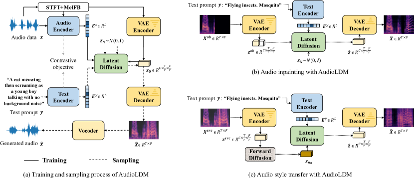
Figure 1: Overview of the AudioLDM system for text-to-audio generation (a). During training, latent diffusion models (LDMs) are conditioned on an audio embedding $\boldsymbol{E}^{x}$ and trained in a continuous space $\boldsymbol{z}_{0}$ learned by VAE. The sampling process uses text embedding $\boldsymbol{E}^{y}$ as the condition. Given a pretrained LDM, zero-shot audio inpainting (b) and style transfer (c) are realized in the reverse diffusion process of LDM. The block Forward Diffusion denotes the process that corrupt data with gaussian noise (see Equation 2).

For previous TTA works, a potential limitation for generation quality is the requirement of large-scale high-quality audio-text data pairs, which are usually not readily available, and where they are available, are of limited quality and quantity (Liu et al., 2022f). To better utilize the low-quality data, several methods for text preprocessing have been proposed (Kreuk et al., 2022; Yang et al., 2022). However, these preprocessing steps limit generation performances by overlooking the relations of sound events  (e.g., a dog is barking at the bark is transformed into dog bark park). By comparison, our proposed method only requires audio data for generative model training, circumvents the challenge of text preprocessing, and performs better than using audio-text paired data, as we will discuss later.

In this work, we present a TTA system, AudioLDM, which achieves high generation quality with continuous LDMs, with good computational efficiency and enables text-conditional audio manipulations. The overview of AudioLDM design for TTA generation and text-guided audio manipulation is shown in Figure 1. Specifically, AudioLDM learns to generate the representation in a latent space encoded by a mel-spectrogram-based variational auto-encoder (VAE). An LDM conditioned on a contrastive language-audio pretraining (CLAP) embedding is developed for VAE latent generation. By leveraging the audio-text-aligned embedding space in CLAP, we remove the requirement for paired audio-text data during training LDM, as the condition for VAE latent generation can directly come from the audio itself. We demonstrate that training an LDM with audio only can be even better than training with audio-text data pairs. The proposed AudioLDM achieves leading TTA performance on the AudioCaps dataset with a Freshet distance (FD) of $23.31$, outperforming the DiffSound baseline (FD of $47.68$) by a large margin. Our system also enables zero-shot audio manipulations in the sampling process. In summary, our contributions are as follows:

• We demonstrate the first attempt to develop a continuous LDM for TTA generation. Our AudioLDM method outperforms existing methods in both subjective evaluation and objective metrics.

• We utilize CLAP embeddings to enable TTA generation without using language-audio pairs to train LDMs.

• We experimentally show that using audio only data in LDM training can obtain a high-quality and computationally efficient TTA system.

• We show that our proposed TTA system can perform text-guided audio styles manipulation, such as audio style transfer, super-resolution, and inpainting, without fine-tuning the model on a specific task.

2 Related Work

Text-to-Audio Generation has gained a lot of attention recently. Two works (Yang et al., 2022; Kreuk et al., 2022) explore how to learn audio representations in a discrete space given a natural language description, and then decode the representations to the audio waveform. Since both works require audio-text paired data for training the latent generation model, they have both proposed methods to address the issues of low quality and scarcity of paired data.

DiffSound (Yang et al., 2022) consists of a text encoder, a decoder, a vector-quantized variational autoencoder (VQ-VAE), and a vocoder. To alleviate the scarcity of audio-text paired data, they propose a mask-based text generation strategy (MBTG) for generating text descriptions from audio labels. For example, the label dog bark, a man speaking will be represented as [M] [M] dog bark [M] man speaking [M], where [M] represent the mask token. However, the text generated by MBTG still only includes the label information, which might potentially limit model performance.

AudioGen (Kreuk et al., 2022) uses a Transformer-based decoder to learn to generate the target discrete tokens that are directly compressed from the waveform. AudioGen is trained on $10$ datasets and proposes data augmentation methods to enhance the diversity of training data. When creating the language-audio pairs, they pre-process the language descriptions to labels to better match the class-label annotation distribution and simplify the task. For example, the text description a dog is barking at the park is transformed to dog bark park. For data augmentation, they mix audio samples according to various signal-to-noise ratios and concatenate the transformed language descriptions. This means that the detailed text descriptions showing the spatial and temporal relationships are discarded.

Diffusion Models (Ho et al., 2020; Song et al., 2021) have achieved state-of-the-art sample quality in tasks such as image generation (Dhariwal & Nichol, 2021; Ramesh et al., 2022; Saharia et al., 2022), image restoration (Saharia et al., 2021), speech generation (Chen et al., 2021; Kong et al., 2021b; Leng et al., 2022), and video generation (Singer et al., 2022; Ho et al., 2022). For speech or audio synthesis, diffusion models have been studied for both mel-spectrogram generation (Popov et al., 2021; Chen et al., 2022c) and waveform generation (Lam et al., 2022; Lee et al., 2022; Chen et al., 2022b).

A major concern with diffusion models is that the iterative generation process in a high-dimensional data space will result in a low inference speed. One of the solutions is to employ diffusion models in a small latent space, an approach used, for example, in image generation (Vahdat et al., 2021; Sinha et al., 2021; Rombach et al., 2022). For TTA generation, the audio waveform has redundant information (Liu et al., 2022e, c) that increases modeling complexity and decreases inference speed. To overcome this, DiffSound (Yang et al., 2022) uses text-conditional discrete diffusion models to generate discrete tokens as a compressed representation of mel-spectrograms. However, the quality of the sound generated by their method is limited. In addition, audio manipulation methods are not explored.

3 Text-Conditional Audio Generation

3.1 Contrastive Language-Audio Pretraining

Text-to-image generation models have shown stunning sample quality by utilizing Contrastive Language-Image Pretraining (CLIP) (Radford et al., 2021) for generating the image prior. Inspired by this, we leverage Contrastive Language-Audio Pretraining (CLAP) (Wu et al., 2022) to facilitate TTA generation.

We denote audio samples as $x$ and the text description as $y$. A text encoder $f_{\text{text}}(\cdot)$ and an audio encoder $f_{\text{audio}}(\cdot)$ are used to extract a text embedding $\boldsymbol{E}^{y}\in\mathbb{R}^{L}$ and an audio embedding $\boldsymbol{E}^{x}\in\mathbb{R}^{L}$ respectively, where $L$ is the dimension of CLAP embedding. A recent study (Wu et al., 2022) has explored different architectures for both the text encoder and the audio encoder when training the CLAP model. We follow their result to build an audio encoder based on HTSAT (Chen et al., 2022a), and built a text encoder based on RoBERTa (Liu et al., 2019). We use a symmetric cross-entropy loss as the training objective (Radford et al., 2021; Wu et al., 2022). For details of the training process and the language-audio datasets see Appendix A.

After training the CLAP model, an audio sample $x$ can be transformed into an embedding $\boldsymbol{E}^{x}$ within an aligned audio and text embedding space. The generalization ability of CLAP model has been demonstrated by various downstream tasks such as the zero-shot audio classification (Wu et al., 2022). Then, for unseen language or audio samples, CLAP embeddings also provide cross-modal information.

3.2 Conditional Latent Diffusion Models

The TTA system can generate an audio sample $\hat{x}$ given text description $y$. With probabilistic generative model LDMs, we estimate the true conditional data distribution $q(\boldsymbol{z}_{0}|\boldsymbol{E}^{y})$ with a model distribution $p_{\theta}(\boldsymbol{z}_{0}|\boldsymbol{E}^{y})$, where $\boldsymbol{z}_{0}\in\mathbb{R}^{C\times\frac{T}{r}\times\frac{F}{r}}$ is the prior of an audio sample $x$ in the space formed from the compressed representation of the mel-spectrogram $\boldsymbol{X}\in\mathbb{R}^{T\times F}$, and $\boldsymbol{E}^{y}$ is the text embedding obtained by pretrained text encoder $f_{\text{text}}(\cdot)$ in CLAP. Here, $r$ denotes the compression level, $C$ denotes the channel of the compressed representation, $T$ and $F$ denote the time-frequency dimensions in the mel-spectrogram $\boldsymbol{X}$. With pretrained CLAP to jointly embed the audio and text information, the audio embedding $\boldsymbol{E}^{x}$ and the text embedding $\boldsymbol{E}^{y}$ share a joint cross-modal space. This allows us to provide $\boldsymbol{E}^{x}$ for training the LDMs, while providing $\boldsymbol{E}^{y}$ for TTA generation.

Diffusion models (Ho et al., 2020; Song et al., 2021) consist of two processes: i) a forward process to transform the data distribution into a standard Gaussian distribution with a predefined noise schedule $0<\beta_{1}<\dots<\beta_{n}<\dots\beta_{N}<1$, and ii) a reverse process to gradually generate data samples from the noise according to an inference noise schedule.

In the forward process, at each time step $n\in[1,\dots,N]$, the transition probability is given by:

$$q(\boldsymbol{z}_{n}|\boldsymbol{z}_{n-1}) =\mathcal{N}(\boldsymbol{z}_{n};\sqrt{1-\beta_{n}}\boldsymbol{z}_{n-1},\beta_{n}\boldsymbol{I}),$$ (1)

$$q(\boldsymbol{z}_{n}|\boldsymbol{z}_{0}) =\mathcal{N}(\boldsymbol{z}_{n};\sqrt{\bar{\alpha}_{n}}\boldsymbol{z}_{0},(1-\bar{\alpha}_{n})\boldsymbol{\epsilon}),$$ (2)

where $\boldsymbol{\epsilon}\sim\mathcal{N}(\boldsymbol{0},\boldsymbol{I})$ denotes injected noise, $\alpha_{n}$ is a reparameterization of $1-\beta_{n}$ and $\bar{\alpha}_{n}:=\prod_{s=1}^{n}\alpha_{s}$ represents the noise level at each step. At the final time step $N$, $\boldsymbol{z}_{N}\sim\mathcal{N}(\boldsymbol{0},\boldsymbol{I})$ has a standard isotropic Gaussian distribution. For model optimization, we employ the reweighted noise estimation training objective (Ho et al., 2020; Kong et al., 2021b; Rombach et al., 2022):

$$L_{n}(\theta)=\mathbb{E}_{\boldsymbol{z}_{0},\boldsymbol{\epsilon},n}\left\|\boldsymbol{\epsilon}-\boldsymbol{\epsilon}_{\theta}(\boldsymbol{z}_{n},n,\boldsymbol{E}^{x})\right\|^{2}_{2},$$ (3)

where $\boldsymbol{E}^{x}$ is the embedding of the audio waveform $x$ produced by the pretrained audio encoder $f_{\text{audio}}(\cdot)$ in CLAP. In the reverse process, starting from Gaussian noise distribution $p(\boldsymbol{z}_{N})\sim\mathcal{N}(\boldsymbol{0},\boldsymbol{I})$ and the text embedding $\boldsymbol{E}^{y}$, a denoising process conditioned on $\boldsymbol{E}^{y}$ gradually generates the audio prior $\boldsymbol{z}_{0}$ by the following process:

$$p_{\theta}(\boldsymbol{z}_{0:N}|\boldsymbol{E}^{y}) =p(\boldsymbol{z}_{N})\prod_{t=n}^{N}p_{\theta}(\boldsymbol{z}_{n-1}|\boldsymbol{z}_{n},\boldsymbol{E}^{y})$$ (4)

$$p_{\theta}(\boldsymbol{z}_{n-1}|\boldsymbol{z}_{n},\boldsymbol{E}^{y}) =\mathcal{N}(\boldsymbol{z}_{n-1};\boldsymbol{\mu}_{\theta}(\boldsymbol{z}_{n},n,\boldsymbol{E}^{y}),\boldsymbol{\sigma}_{n}^{2}\boldsymbol{I}).$$ (5)

The mean and variance are parameterized as (Ho et al., 2020):

$$\boldsymbol{\mu}_{\theta}(\boldsymbol{z}_{n},n,\boldsymbol{E}^{y}) =\frac{1}{\sqrt{\alpha_{n}}}(\boldsymbol{z}_{n}-\frac{\beta_{n}}{\sqrt{1-\bar{\alpha}_{n}}}\boldsymbol{\epsilon}_{\theta}(\boldsymbol{z}_{n},n,\boldsymbol{E}^{y}))$$ (6)

$$\boldsymbol{\sigma}_{n}^{2} =\frac{1-\bar{\alpha}_{n-1}}{1-\bar{\alpha}_{n}}\beta_{n}$$ (7)

where $\boldsymbol{\epsilon}_{\theta}(\boldsymbol{z}_{n},n,\boldsymbol{E}^{y})$ is the predicted generation noise, and $\boldsymbol{\sigma}_{1}^{2}=\beta_{1}$. In the training stage, we learn the generation of an audio prior $\boldsymbol{z}_{0}$ given the cross-modal representation $\boldsymbol{E}^{x}$ of an audio sample $x$. Then, in TTA generation, we provide the text embeddings $\boldsymbol{E}^{y}$ to predict the noise $\boldsymbol{\epsilon}_{\theta}(\boldsymbol{z}_{n},n,\boldsymbol{E}^{y})$. Built on the CLAP embeddings, our LDM realizes TTA generation without text supervision in the training stage. We provide the details of network architecture in Appendix B.

3.3 Conditioning Augmentation

In text-to-image generation, diffusion-based models have demonstrated an ability to capture the fine-grained details between objects and backgrounds (Ramesh et al., 2022; Saharia et al., 2022; Liu et al., 2022d). One of the reasons for this success is the large-scale language-image training pairs, such as $400$ million image-text pairs in the LAION dataset (Schuhmann et al., 2021). For TTA generation, it is also desired to generate compositional audio signals whose relationships are consistent with natural language descriptions. However, the scale of available language-audio datasets is not comparable to that of language-image datasets. For data augmentation, AudioGen (Kreuk et al., 2022) use a mixup strategy which mixes pairs of audio samples and concatenates their respective processed text captions to form new paired data. In our work, as shown in Equation 3, we provide the audio only embedding $\boldsymbol{E}^{x}$ as conditioning information when training LDMs, we can implement data augmentation on audio only signals instead of needing to augment language-audio pairs. Specifically, we perform mixup augmentation on audio $x_{1}$ and $x_{2}$ by:

$$x_{1,2}=\lambda x_{1}+(1-\lambda)x_{2},$$ (8)

where $\lambda$ is a scaling factor varying between $\left[0,1\right]$ sampled from a Beta distribution $\mathcal{B}(5,5)$ (Gong et al., 2021). Here we do not need to consider the corresponding text description $y_{1,2}$, since text information is not needed during LDM training. By mixing audio pairs, we increase the number of training data pairs $(\boldsymbol{z}_{0},\boldsymbol{E}^{x})$ for LDMs, which makes LDMs robust to CLAP embeddings. In the sampling process, given the text embedding $\boldsymbol{E}^{y}$ from unseen language descriptions, LDMs are expected to generate the corresponding audio prior $\boldsymbol{z}_{0}$.

3.4 Classifier-free Guidance

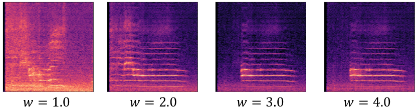
Figure 2: The samples generated with different scales of the classifier-free guidance. The text prompt is “A cat is meowing”.

For diffusion models, controllable generation can be achieved by introducing guidance at each sampling step. After classifier guidance (Song et al., 2021; Nichol & Dhariwal, 2021), classifier-free guidance (Ho & Salimans, 2021; Nichol et al., 2021) (CFG) has been the state-of-the-art technique for guiding diffusion models. During training, we randomly discard our condition $\boldsymbol{E}^{x}$ with a fixed probability, e.g., $10\%$ to train both the conditional LDMs $\boldsymbol{\epsilon}_{\theta}(\boldsymbol{z}_{n},n,\boldsymbol{E}^{x})$ and the unconditional LDMs $\boldsymbol{\epsilon}_{\theta}(\boldsymbol{z}_{n},n)$. In generation, we use text embedding $\boldsymbol{E}^{y}$ as condition and perform sampling with a modified noise estimation $\hat{\boldsymbol{\epsilon}}_{\theta}(\boldsymbol{z}_{n},n,\boldsymbol{E}^{y})$:

$$\hat{\boldsymbol{\epsilon}}_{\theta}(\boldsymbol{z}_{n},n,\boldsymbol{E}^{y})=w\boldsymbol{\epsilon}_{\theta}(\boldsymbol{z}_{n},n)+(1-w)\boldsymbol{\epsilon}_{\theta}(\boldsymbol{z}_{n},n,\boldsymbol{E}^{y}),$$ (9)

where $w$ determines the guidance scale. Compared with AudioGen (Kreuk et al., 2022), we have two differences. First, they leverage CFG on a transformer-based auto-regressive model, while our LDMs retain the theoretical formulation behind the CFG (Ho & Salimans, 2021). Second, our text embedding $\boldsymbol{E}^{y}$ is extracted from unprocessed natural language and therefore enables CFG to make use of the detailed text descriptions as guidance for audio generation. However, AudioGen removed the text details showing spatial or temporal relationships with text preprocessing methods.

3.5 Decoder

We use VAE to compress the mel-spectrogram $\boldsymbol{X}\in\mathbb{R}^{T\times F}$ into a small latent space $\boldsymbol{z}\in\mathbb{R}^{C\times\frac{T}{r}\times\frac{F}{r}}$, where $r$ is the compression level of the latent space. Our VAE is composed of an encoder and a decoder with stacked convolutional modules. In the training objective, we adopt a reconstruction loss, an adversarial loss, and a Gaussian constraint loss. We provide the detailed architecture and training methods in Appendix C. In the sampling process, the decoder is used to reconstruct the mel-spectrogram $\boldsymbol{\hat{X}}$ from the audio prior $\boldsymbol{\hat{z}}_{o}$ generated from LDMs. To explore a compression level $r$ that achieves a small latent space for LDMs without sacrificing sample quality, we test a group of values $r\in\left[1,2,4,8,16\right]$, and take $r\texttt{=}4$ as our default setting because of its high computational efficiency and generation quality. Moreover, as we conduct conditioning augmentation for LDMs, we implement data augmentation with Equation 9 for VAE as well in order to guarantee the reconstruction quality of generated compositional samples. For vocoder, we employ HiFi-GAN (Kong et al., 2020a) to generate the audio sample $\hat{x}$ from the reconstructed mel-spectrogram $\boldsymbol{\hat{X}}$. The training details are shown in Appendix D.

4 Text-Guided Audio Manipulation

Style Transfer Given a source audio sample $x^{src}$, we can calculate its noisy latent representation $\boldsymbol{z}_{n_{0}}$ with a predefined time step $n_{0}\leq N$ according to the forward process shown in Equation 2. By utilizing $\boldsymbol{z}_{n_{0}}$ as the starting point of the reverse process of a pretrained AudioLDM model, we enable the manipulation of audio $x^{src}$ with text input $y$ with a shallow reverse process $p_{\theta}(\boldsymbol{z}_{0:n_{0}}|\boldsymbol{E}^{y})$:

$$p_{\theta}(\boldsymbol{z}_{0:n_{0}}|\boldsymbol{E}^{y}) =p(\boldsymbol{z}_{n_{0}})\prod_{n=1}^{n_{0}}p_{\theta}(\boldsymbol{z}_{n-1}|\boldsymbol{z}_{n},\boldsymbol{E}^{y}),$$ (10)

where $n_{0}$ controls the manipulation results. If we define a $n_{0}\approx N$, the information provided by source audio will not be retained and the manipulation would be similar to TTA generation. We show the effect of $n_{0}$ in Figure 3, where larger manipulations can be seen in the setting of $n_{0}=3N/4$.

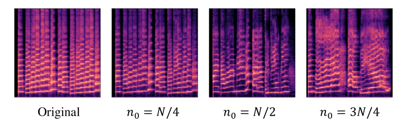
Figure 3: The manipulation result with different starting points $n_{0}$ of the shallow reverse process. The original signal is Trumpet, and the text prompt for style transfer is Children Singing.

Inpainting and Super-Resolution Both audio inpainting and audio super-resolution refer to generating the missing part given the observed part $x^{ob}$. We explore these tasks by incorporating the observed part in latent representation $\boldsymbol{z}^{ob}$ into the generated latent representation $\boldsymbol{z}$. Specifically, in reverse process, starting from $p(\boldsymbol{z}_{N})\sim\mathcal{N}(\boldsymbol{0},\boldsymbol{I})$, after each inference step shown in Equation 5, we modify the generated $\boldsymbol{z}_{n-1}$ with:

$$\boldsymbol{z}^{\prime}_{n-1} =(1-\boldsymbol{m})\odot\boldsymbol{z}_{n-1}+\boldsymbol{m}\odot\boldsymbol{z}^{ob}_{n-1},$$ (11)

where $\boldsymbol{z}^{\prime}$ is the modified latent representation, $\boldsymbol{m}\in\mathbb{R}^{\frac{T}{r}\times\frac{F}{r}}$ denotes an observation mask in latent space, $\boldsymbol{z}^{ob}_{n-1}$ is obtained by adding noise on $\boldsymbol{z}^{ob}$ with the forward process shown by Equation 2.

The values of observation mask $\boldsymbol{m}$ depend on the observed part of a mel-spectrogram $\boldsymbol{X}$. As we adopt a convolutional structure in VAE to learn the latent representation $\boldsymbol{z}$, we can roughly retain the spatial correspondency in mel-spectrogram, as it is shown in Figure 7 in Appendix C. Therefore, if a time-frequency bin $\boldsymbol{X}_{t,f}$ is observed, we set the observation mask $\boldsymbol{m}_{\frac{t}{r},\frac{f}{r}}$ in latent space as $1$. By using $\boldsymbol{m}$ to denote the generation part and observation part in $\boldsymbol{z}$, according to Equation 11, we can generate the missing information conditioned on the text prompt with TTA models, while retaining the ground-truth observation $\boldsymbol{z}^{ob}$.

Model	Text Data	Use CLAP	Params	Duration (h)	FD $\downarrow$	IS $\uparrow$	KL $\downarrow$	FAD $\downarrow$	OVL $\uparrow$	REL $\uparrow$
Ground truth	-	-	-	-	-	-	-	-	$83.61_{\pm 1.1}$	$80.11_{\pm 1.2}$
DiffSound† (Yang et al., 2022)	✓	✗	$400$M	$5420$	$47.68$	$4.01$	$2.52$	$7.75$	$45.00_{\pm 2.6}$	$43.83_{\pm 2.3}$
AudioGen† (Kreuk et al., 2022)	✓	✗	$285$M	$8067$	-	-	$2.09$	$3.13$	-	-
AudioLDM-S-Full-RoBERTa	✓	✗	$181$M	$145$	$32.13$	$4.02$	$3.25$	$5.89$	-	-
AudioLDM-S	✗	✓	$181$M	$145$	$29.48$	$6.90$	$1.97$	$2.43$	$63.41_{\pm 1.4}$	$64.83_{\pm 0.9}$
AudioLDM-L	✗	✓	$739$M	$145$	$27.12$	$7.51$	$1.86$	$2.08$	$64.30_{\pm 1.6}$	$64.72_{\pm 1.6}$
AudioLDM-S-Full	✗	✓	$181$M	$8886$	$23.47$	$7.57$	$1.98$	$2.32$	-	-
AudioLDM-L-Full	✗	✓	$739$M	$8886$	$\mathbf{23.31}$	$\mathbf{8.13}$	$\mathbf{1.59}$	$\mathbf{1.96}$	$\mathbf{65.91}_{\pm 1.0}$	$\mathbf{65.97}_{\pm 1.6}$

Table 1: The comparison between AudioLDM and baseline TTA generation models. Evaluation is conducted on AudioCaps test set. The symbol ^† marks industry-level computation. DiffSound is trained on $32$ V$100$ GPUs and AudioGen is trained on $64$ A$100$ GPUs, while AudioLDM models are trained on a single GPU, RTX $3090$ or A$100$. The AS and AC stand for AudioSet and AudioCaps datasets respectively. The results of AudioGen are employed from  (Kreuk et al., 2022) since their implementation has been not publicly available.

5 Experiments

Training dataset The datasets we used in this paper includes AudioSet (AS) (Gemmeke et al., 2017), AudioCaps (AC) (Kim et al., 2019), Freesound (FS), and BBC Sound Effect library (SFX). AS is currently the largest audio dataset, with $527$ labels and over $5,000$ hours of audio data. AC is a much smaller dataset with around $49,000$ audio clips and text descriptions. Most of the data in AudioSet and AudioCaps are in-the-wild audio from YouTube, so the quality of the audio is not guaranteed. To expand the dataset, especially with high-quality audio data, we crawl the data from the FreeSound and BBC SFX datasets, which have a wide range of categories such as music, speech, and sound effects. We show our detailed data processing methods and training configuration in Appendix E.

Evaluation dataset We evaluate the model on both AC and AS. Each audio clip in AC has $5$ text captions. We generate the evaluation set by randomly selecting one of them as text condition. Because the authors of AC intentionally remove the audio with the label related to music (Kim et al., 2019), to evaluate model performance with a wider range of sound, we randomly select $10\%$ audio samples from AS as another evaluation set. Since AS does not contain text descriptions, we use the concatenation of labels as text descriptions, such as Speech, hip hop music, and crowd cheering.

Evaluation methods We perform both objective evaluation and human subjective evaluation. The main metrics we use for objective evaluation include frechet distance (FD), inception score (IS), and kullback–leibler (KL) divergence. Similar to the frechet inception distance in image generation, the FD in audio indicates the similarity between generated samples and target samples. IS is effective in evaluating both sample quality and diversity. KL is measured at a paired sample level and averaged as the final result. All of these three metrics are built upon a state-of-the-art audio classifier PANNs (Kong et al., 2020b). To compare with (Kreuk et al., 2022), we also adopt the frechet audio distance (FAD) (Kilgour et al., 2019). FAD has a similar idea to FD but it uses VGGish (Hershey et al., 2017) as a classifier which may have inferior performance than PANNs. To better measure the generation quality, we choose FD as the main evaluation metric in this paper. For subjective evaluation, we recruit six audio professionals to carry on a rating process following (Kreuk et al., 2022; Yang et al., 2022). Specifically, the generated samples are rated based on i) overall quality (OVL); and ii) relevance to the input text (REL) between a scale of $1$ to $100$. We include the details of human evaluation in Appendix E. We open-source our evaluation pipeline to facilitate reproducibility.

Models We employ two recently proposed TTA systems, DiffSound (Yang et al., 2022) and AudioGen (Kreuk et al., 2022) as our baseline models. DiffSound is trained on AS and AC datasets with around $400$M parameters. AudioGen is trained on AS, AC, and eight other datasets with around $285$M parameters. Since AudioGen has not released publicly available implementation, we reuse the KL and FAD results reported in their paper. We train two AudioLDM models. One is a small model named AudioLDM-S, which has $181$M parameters, and the other is a large model named AudioLDM-L with $739$M parameters. We describe the details of UNet architecture in Appendix B. To demonstrate the advantage of our method, we simply train these two models only with the AC dataset. Moreover, to explore the effect of the scale of training data, we develop an AudioLDM-L-Full model which is trained on AC, AS, FreeSound, and BBC SFX datasets.

5.1 Results

We show the main evaluation results on the AC test set in Table 1. Given the single training dataset AC, AudioLDM-S can achieve better generation results than the baseline models on both objective and subjective evaluations, even with smaller model size. By expanding model capacity with AudioLDM-L, we further improve the overall results. Then, by incorporating AS and the two other datasets into training, our model AudioLDM-L-Full achieves the best quality, with an FD of $23.31$. Although RoBERTa and CLAP have the same text encoder structure, CLAP has an advantage in that it decouples audio-text relationship learning from generative model training. This decoupling is intuitive as CLAP has already modelled the relationship between audio and text by aligning their embedding spaces. On the other hand, AudioLDM-S-Full-RoBERTa, in which the text encoder only represents textual information, requires the model to learn the text-audio relationships while simultaneously learning the audio generation process. Additionally, our CLAP-based method allows for model training using audio-only data. Therefore, using Roberta without pretraining with CLAP may increase the difficulty of training.

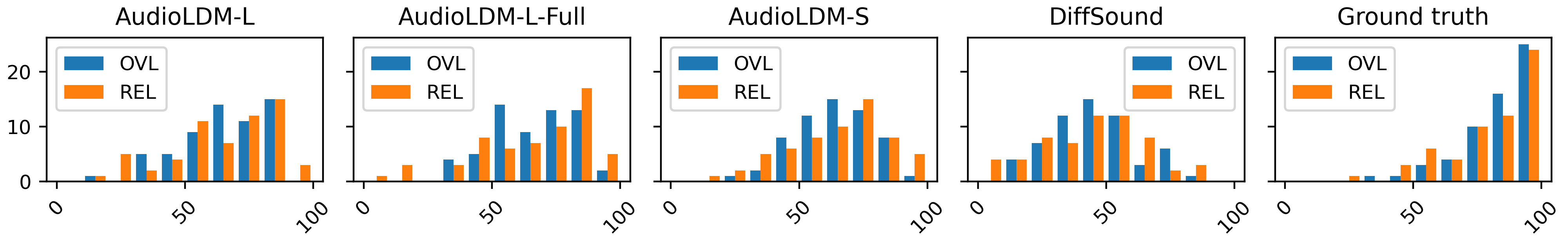
Figure 4: The histogram of the human evaluation result. The horizontal axis and vertical axis represent the rating score and frequency, respectively. OVL denotes the overall quality of audio files and REL denotes the relation between text and generated audio. Both OVL and REL are scored on a scale of $1$ to $100$. Scores on each evaluation file are averaged among all the raters.

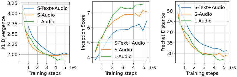
Figure 5: The comparison of various evaluation metrics evaluated in the training process of i) AudioLDM-S trained with text embedding (S-Text+Audio) ii) AudioLDM-S (S-Audio), and iii) AudioLDM-L (L-Audio).

Our human evaluation shows a similar trend as other evaluation metrics. Our proposed methods have OVL and REL of around $64$, outperforming DiffSound with OVL of $45.00$ and REL of $43.83$ by a large margin. On the AudioLDM model size, we notice that the larger model is advantageous for the overall audio qualities. After scaling up the training data, both OVL and REL show significant improvements. Figure 4 shows the score statistic of different models averaged between all the raters. We notice our model is more concentrated on the higher scores compared with DiffSound. Our spam cases, which are randomly selected real recordings, show high scores, indicating the rating result is reliable.

To perform the evaluation on audio data that could include music, we further evaluate our model on the AS evaluation set. We compare our method with DiffSound and show the results in Table 2. Our three AudioLDM models show a similar trend as they perform on the AC test set. We can outperform the DiffSound baseline by a large margin on all the metrics.

Model	FD $\downarrow$	IS $\uparrow$	KL $\downarrow$
DiffSound	$50.40$	$4.19$	$3.63$
AudioLDM-S	$28.08$	$6.78$	$2.51$
AudioLDM-L	$27.51$	$7.18$	$2.49$
AudioLDM-L-Full	$\mathbf{24.26}$	$\mathbf{7.67}$	$\mathbf{2.07}$

Table 2: The evaluation results on the AudioSet evaluation set.

Conditioning Information As we train LDMs conditioned on the audio embedding $\boldsymbol{E}^{x}$ but provide the text embedding $\boldsymbol{E}^{y}$ to LDMs in TTA generation, a natural concern is that if stronger results could be achieved by directly using the text embedding as training condition. We conduct experiments and show the results in Table 3. For a fair comparison, we also conduct data augmentation and we adopt the strategy from AudioGen. Specifically, we use the same mixing method for audio pairs shown in Section 3.3, and concatenate two text captions as conditioning information. Table 3 shows by training LDMs on $\boldsymbol{E}^{x}$, we can achieve better results than training with $\boldsymbol{E}^{y}$.

Model	Text	Audio	FD $\downarrow$	IS $\uparrow$	KL $\downarrow$
AudioLDM-S	✓	✓	$31.26$	$6.35$	$2.01$
AudioLDM-S	✗	✓	$\mathbf{29.48}$	$\mathbf{6.90}$	$\mathbf{1.97}$
AudioLDM-S-Full	✓	✓	$27.20$	$7.52$	$2.38$
AudioLDM-S-Full	✗	✓	$\mathbf{23.47}$	$\mathbf{7.57}$	$\mathbf{1.98}$
AudioLDM-L-Full	✓	✓	$25.79$	$7.95$	$2.26$
AudioLDM-L-Full	✗	✓	$\mathbf{23.31}$	$\mathbf{8.13}$	$\mathbf{1.59}$

Table 3: The comparison between text embedding and audio embedding as conditioning information on the training of LDMs.

We believe the primary reason for the result in Table 3 is that text embedding cannot represent the generation target as good as audio embedding. Firstly, due to the ambiguity and complexity of sound, the text caption is difficult to be accurate and comprehensive. Different human annotators may have different perceptions and descriptions over the same audio, which make training with text-audio pair less stable than with audio only. Moreover, some of the captions are at a highly-abstracted level and cannot correctly describe the audio content. For example, there is an audio in the BBC SFX dataset with caption Boats: Battleships-5.25 conveyor space, which is even difficult for humans to imagine how it sounds. This quality of language-audio pairs may hinder model optimization. By comparison, if we use $\boldsymbol{E}^{x}$ from CLAP latents as a condition, it is extracted directly from the audio signal and is aligned with ideally the best text caption, which enables us to provide strong conditioning information to LDMs without considering the noisy labeled text description. Figure 5 shows sample quality as a function of training progress. We notice that i) training with audio embedding can lead to significantly better results than text embedding throughout the entire training process; and ii) larger models may converge more slowly but can achieve better final performance.

Compression Level We study the effect of compression level $r$ on generation quality. Table 4 shows the performance comparison with $r\texttt{=}4,8,16$. We observe a decreasing trend with the increase of compression levels. Nevertheless, in the setting of $r\texttt{=}16$ where we compress the $64$-band mel-spectrogram into only $4$ dimensions in the frequency axis, our performance is still on par with AudioGen on KL, and better than DiffSound on all the metrics.

Model	$r$	FD $\downarrow$	IS $\uparrow$	KL $\downarrow$
AudioLDM-S	$4$	$\mathbf{29.48}$	$\mathbf{6.90}$	$\mathbf{1.97}$
AudioLDM-S	$8$	$33.50$	$6.13$	$2.04$
AudioLDM-S	$16$	$34.32$	$5.68$	$2.09$

Table 4: The effect of the compression level on AudioLDM.

If we set the compression level as $r\texttt{=}1$, which means we directly generate mel-spectrogram from CLAP embeddings, the training process is difficult to implement on a single RTX $3090$ GPU. Similar results happen on $r\texttt{=}2$. Moreover, the inference speed will be low with $r\texttt{=}1,2$. In our studies, $r\texttt{=}4$ achieves high generation quality while reducing the computational load to a reasonable level. Hence, we use it as the default setting in our experiments.

Text-Guided Audio Manipulation We show the performance of our text-guided audio manipulation methods on two tasks: super-resolution and inpainting. Specifically, for super-resolution, we upsample the audio signal from $8$ kHz to $16$ kHz sampling rate. For the inpainting task, we remove the audio signal between $2.5$ and $7.5$ seconds and refill this part by inpainting. Since most studies on audio super-resolution work on speech signal (Liu et al., 2021a, 2022a), we demonstrate our results on both AudioCaps, and a speech dataset VCTK (Yamagishi et al., 2019), which is a multi-speaker speech dataset. For super-resolution, we employ two models AudioUNet (Kuleshov et al., 2017) and NVSR (Liu et al., 2022a) as baseline models, and employ log-spectral distance (LSD) (Wang & Wang, 2021) as the evaluation metric for comparison. For the inpainting task, we use FAD as a metric and establish a baseline for this task.

Task	Super-resolution		Inpainting
Dataset	AudioCaps	VCTK	AudioCaps
Unprocessed	$2.76$	$2.15$	$10.86$
Kuleshov et al. (2017)	-	$1.32$	-
Liu et al. (2022a)	-	$\mathbf{0.78}$	-
AudioLDM-S	$1.59$	$1.12$	$2.33$
AudioLDM-L	$\mathbf{1.43}$	$0.98$	$\mathbf{1.92}$

Table 5: Performance comparisons on zero-shot super-resolution and inpainting, which are evaluated by LSD and FAD, respectively.

Table 5 shows that AudioLDM can outperform the strong AudioUNet baseline, but the result is not as good as NVSR (Liu et al., 2022a). Recall that AudioLDM is a model trained on a diverse set of audio signals, including those with heavy background noise. This can lead to the presence of white noise or other non-speech sound events in the output of our super-resolution process, potentially reducing performance. Nevertheless, our contribution could open the door to achieving text-guided audio manipulation with the TTA system in a zero-shot way. Further improvements could be expected based on our benchmark results. We provide several samples of our results in Appendix I.

5.2 Ablation Study

Table 6 shows the result of our ablation study on AudioLDM-S. By simplifying the attention mechanism in UNet into a one-layer multi-head self-attention (w. Simple attn), the performance in each metric will have a notable decrease, which indicates complex attention mechanism is preferred. Also, we notice the widely used balanced sampling strategy (Gong et al., 2021; Liu et al., 2022b) in audio classification does not show improvement in TTA (w. Balance samp). Conditional augmentation (see Section 3.3) shows improvement in the subjective evaluation, but it does not show improvement in the objective evaluation metrics (w. Cond aug). The reason could be that conditioning augmentation generates training data that is not representative of the AudioCaps dataset, resulting in model outputs that are not well-aligned with the evaluation data, ultimately leading to lower metric scores. Nevertheless, conditioning augmentation can improve two subjective metrics and we still recommend using it as a data augmentation technique.

Setting	FD$\downarrow$	IS$\uparrow$	KL$\downarrow$	OVL $\uparrow$	REL $\uparrow$
AudioLDM-S	$\mathbf{29.48}$	$\mathbf{6.90}$	$\mathbf{1.97}$	$63.41$	$64.83$
w. Simple attn	$33.12$	$6.15$	$2.09$	-	-
w. Balance samp	$34.05$	$6.21$	$2.16$	-	-
w. Cond aug	$31.88$	$6.25$	$2.02$	$\mathbf{64.49}$	$\mathbf{65.01}$

Table 6: The ablation study on the attention mechanism, the balance sampling technique for training data, and the conditioning augmentation algorithm.

DDIM Sampling Step The number of inference steps in the reverse process of DDPMs can directly affect the generation quality (Ho et al., 2020; Song et al., 2021). Generally, the sample quality can be improved with an increase in the number of sampling steps and computational load at the same time. We explore the effect of the DDIM (Song et al., 2020) sampling steps on our latent diffusion model. Table 7 shows that more sampling steps lead to better quality. With enough sampling steps such as $100$, the gain of adding sampling steps becomes less significant. The result of $200$ steps is only slightly better than that of $100$ steps.

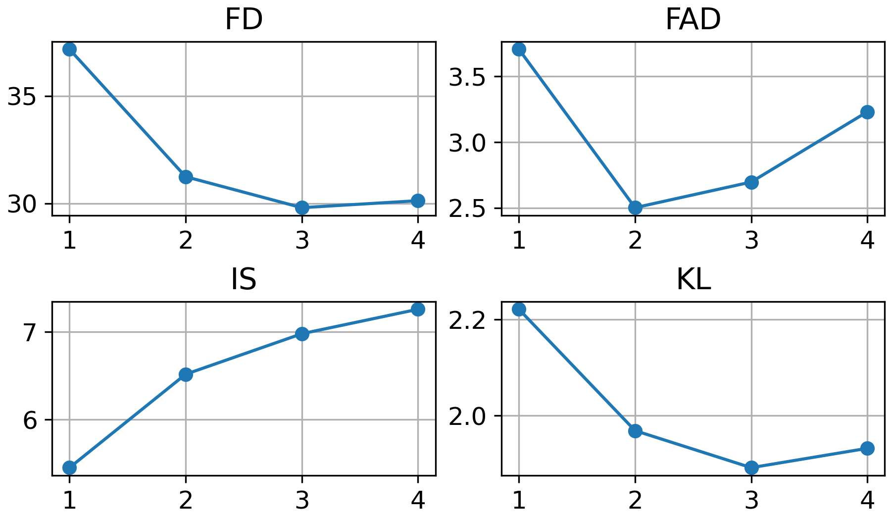
Figure 6: The comparison between different classifier-free guidance scales (on the horizontal axis) for the AudioLDM-S model trained on AudioCaps.

DDIM steps	$10$	$25$	$50$	$100$	$200$
FD	$55.84$	$42.84$	$35.71$	$30.17$	$\mathbf{29.48}$
IS	$4.21$	$5.91$	$6.51$	$6.85$	$\mathbf{6.90}$
KL	$2.47$	$2.12$	$2.01$	$\mathbf{1.94}$	$1.97$

Table 7: Effect of sampling steps of LDMs with a DDIM sampler.

Guidance Scale represents a trade-off between conditional generation quality and sample diversity. A suitable guidance scale can improve the consistency between generated samples and conditioning information at an acceptable cost of generation diversity. We show the effect of guidance scale $w$ on TTA in Figure 6. When $w=3$, we achieve the best results in both FD and KL, but not in FAD. We suppose the reason is the audio classifier in FAD is not as good as FD, as mentioned in Section 5. In this case, the improvement in the adherence to detailed language description may become misleading information to the classifier in FAD. Considering previous studies report FAD results instead of FD, we set $w=2$ for comparison, but also provide detailed effects of $w$ on FAD, FD, IS, and KL, respectively.

Case Study We conduct case study and show the generated results in Appendix I, including style transfer (see Figure 9-11), super-resolution (see Figure 12), inpainting (see Figure 13-14), and text-to-audio generation (see Figure 15-22). Specifically, for text-to-audio, we demonstrate the controllability of AudioLDM, including the control of the acoustic environment, material, sound event, pitch, musical genres, and temporal orders.

6 Conclusions

We have presented a new method AudioLDM for text-to-audio (TTA) generation, with contrastive language-audio pretraining (CLAP) models and latent diffusion models (LDMs). Our method is advantageous in generation quality, computational efficiency, and audio manipulations. With a single training dataset AudioCaps and a single GPU, AudioLDM achieves SOTA generation quality evaluated by both subjective and objective metrics. Moreover, AudioLDM enables zero-shot text-guided audio style transfer, super-resolution, and inpainting.

7 Acknowledgement

We would like to thank James King and Jinhua Liang for the useful discussion on the latent diffusion model. This research was partly supported by the British Broadcasting Corporation Research and Development (BBC R&D), Engineering and Physical Sciences Research Council (EPSRC) Grant EP/T019751/1 “AI for Sound”, and a PhD scholarship from the Centre for Vision, Speech and Signal Processing (CVSSP), Faculty of Engineering and Physical Science (FEPS), University of Surrey. For the purpose of open access, the authors have applied a Creative Commons Attribution (CC BY) license to any Author Accepted Manuscript version arising.

Appendix

A Contrastive Language-Audio Pretraining

We follow the pipeline of the contrastive language-audio pretraining (CLAP) models proposed by (Wu et al., 2022) to capture the similarity between text and audio, and project them into joint latent space. The training dataset includes the currently largest public dataset LAION-Audio-$630$K, the AudioSet dataset whose text caption is augmented with keyword-to-caption by T$5$ model (Raffel et al., 2020), the AudioCaps dataset and the Clotho dataset (Drossos et al., 2020). The LAION-Audio-$630$K dataset contains $633,526$ language-audio pairs and $4325.39$ hours of audio samples. The AudioSet dataset contains $1,912,024$ pairs and $463.48$ hours of audio samples. The AudioCaps dataset contains $49,274$ pairs and $136.87$ hours of audio samples. The Clotho dataset contains $3,839$ pairs and $23.99$ hours of audio samples. These datasets contain various natural sounds, audio effects, music and human activity.

Given the audio sample $x$ and the text data $y$, we use an audio encoder and a text encoder to extract their embedding $\boldsymbol{E}^{x}\in\mathbb{R}^{L}$ and $\boldsymbol{E}^{y}\in\mathbb{R}^{L}$ respectively, where $L$ is set as $512$. We build the audio encoder based on HTSAT (Chen et al., 2022a) and the text encoder based on RoBERTa (Liu et al., 2019). The symmetric cross-entropy loss used to train these contrastive encoders is:

$$L_{s} =\frac{1}{2D}\sum^{D}_{i=1}(l_{1}+l_{2}),$$ (12)

$$l_{1} =\log\frac{\exp(\boldsymbol{E}^{x}_{i}\cdot\boldsymbol{E}^{y}_{i}/\tau)}{\sum^{N}_{i=1}\exp(\boldsymbol{E}^{x}_{i}\cdot\boldsymbol{E}^{y}_{j}/\tau)},$$ (13)

$$l_{2} =\log\frac{\exp(\boldsymbol{E}^{y}_{i}\cdot\boldsymbol{E}^{x}_{i}/\tau)}{\sum^{N}_{i=1}\exp(\boldsymbol{E}^{y}_{i}\cdot\boldsymbol{E}^{x}_{j}/\tau)}),$$ (14)

where $\tau$ is a learnable temperature parameter and $D$ is the batch size.

B Latent Diffusion Model

We adopt the UNet backbone of StableDiffusion (Rombach et al., 2022) as the basic architecture of LDM for AudioLDM. As shown in Equation 5, the UNet model is conditioned on both the time step $t$ and the CLAP embedding $\boldsymbol{E}$. We map the time step into a one-dimensional embedding and then concatenate it with $\boldsymbol{E}$ as conditioning information. Since our condition vector is only one-dimensional, we do not use the cross-attention mechanism in StableDiffusion for conditioning. Instead, we directly use the feature-wise linear modulation layer (Perez et al., 2018) to merge conditioning information with the feature map of the UNet convolution block. The UNet backbone we use has four encoder blocks, a middle block, and four decoder blocks. With a basic channel number of $c_{u}$, the channel dimensions of encoder blocks are $[c_{u},2c_{u},3c_{u},5c_{u}]$. The channel dimensions of decoder blocks are the reverse of encoder blocks, and the channel of the middle block has $5c_{u}$ dimensions. We add an attention block in the last three encoder blocks and the first three decoder blocks. Specifically, we add two multi-head self-attention layers with a fully-connected layer in the middle as the attention block. The number of heads is determined by dividing the embedding dimension of the attention block with a parameter $c_{h}$. We set AudioLDM-S and AudioLDM-L with $c_{u}\texttt{=}128,c_{h}\texttt{=}32$, and $c_{u}\texttt{=}256,c_{h}\texttt{=}64$, respectively. In the forward process, we use $N=1000$ steps. A linear noise schedule from $\beta_{1}=0.0015$ to $\beta_{N}=0.0195$ is used. In sampling, we employ the DDIM (Song et al., 2020) sampler with $200$ sampling steps. For classifier-free guidance, a guidance scale $w$ of $2.0$ is used in Equation 9.

C Variational Autoencoder

We compress the mel-spectrogram $\boldsymbol{X}\in\mathbb{R}^{T\times F}$ of $x$ into a small continuous space $\boldsymbol{z}\in\mathbb{R}^{C\times\frac{T}{r}\times\frac{F}{r}}$ with a convolutional VAE, where $T$ and $F$ is the time and frequency dimension size respectively, $C$ is the channel number of the latent encoding, and $r$ is the compression level (downsampling ratio) of latent space. Both the encoder $\mathcal{E}(\cdot)$ and the decoder $\mathcal{D}(\cdot)$ are composed of stacked convolutional modules. In this way, VAE encoder could preserve the spatial correspondancy between mel-spectrogram and latent space, as it is shown in Figure 7. Each module is formed by ResNet blocks (Kong et al., 2021a) which are made up of convolutional layers and residual connections. The encoding $\boldsymbol{z}$ will be evenly split into two parts, $\boldsymbol{z}_{\boldsymbol{\mu}}$ and $\boldsymbol{z}_{\boldsymbol{\sigma}}$, with shape $(\frac{C}{2},\frac{T}{r},\frac{F}{r})$, representing the mean and variance of the VAE latent space. The input of the decoder is a stochastic encoding $\boldsymbol{\hat{z}}=\boldsymbol{\hat{z}}_{\boldsymbol{\mu}}+\boldsymbol{\hat{z}}_{\boldsymbol{\sigma}}\cdot\boldsymbol{\epsilon},\boldsymbol{\epsilon}\sim\mathcal{N}(0,I)$. During generation, the decoder will be used to reconstruct the mel-spectrogram given the generated latent representations.

We employ three loss functions in our training objective: the mel-spectrogram reconstruction loss, adversarial losses, and a gaussian constraint loss. The reconstruction loss calculates the mean absolute error between the input sample $\boldsymbol{X}\in\mathbb{R}^{T\times F}$ and the reconstructed mel-spectrogram $\hat{\boldsymbol{X}}\in\mathbb{R}^{T\times F}$. The adversarial losses are employed to enhance the reconstruction quality. Specifically, we adopt the PatchGAN (Isola et al., 2017) as our discriminator, which will divide the input image into small patches and predict whether each patch is real or fake by outputting a matrix of logits. The PatchGAN discriminator is trained to maximize the logits of correctly identifying real patches while minimizing the logits of incorrectly identifying fake patches. We also apply the gaussian constraint on the latent space of VAE. By enforcing a gaussian constraint on the latent space, the VAE is encouraged to learn a continuous, structured latent space, rather than a disorganized one. This can help the VAE to better capture the underlying structure of the data, which can result in more stabilized and accurate reconstructions (Kingma & Welling, 2013).

We train our VAE using the Adam optimizer (Kingma & Ba, 2014) with a learning rate of $4.5\times 10^{-6}$ and a batch size of six. The audio data we use includes AudioSet, AudioCaps, Freesound, and BBC SFX. We perform experiments with three compression-level settings $r\texttt{=}4,8,16$, for which the latent channels are $C=8,16,32$, respectively. VAEs in all three settings are trained with at least $1.5$M steps on a single NVIDIA RTX 3090 GPU. To stabilize training, we do not apply the adversarial loss in the first $50$K training steps. We apply the mixup (Kong et al., 2020b) strategy for data augmentation.

Table 8 shows the reconstruction performance of our VAE model with different values of $r$. All three settings achieve comparable metrics score with the GT Mel + Vocoder setting, indicating the autoencoder can perform reliable mel-spectrogram encoding and decoding.

Setting	PSNR$\uparrow$	SSIM$\uparrow$	FD$\downarrow$	IS$\uparrow$	KL$\downarrow$
GT Mel + Vocoder	$25.41$	$0.86$	$8.76$	$10.71$	$0.23$
Compressionr=4	$25.38$	$0.86$	$9.02$	$10.67$	$0.23$
Compressionr=8	$25.14$	$0.84$	$9.68$	$10.50$	$0.25$
Compressionr=16	$24.87$	$0.82$	$9.90$	$9.84$	$0.29$

Table 8: The objective metrics of VAE reconstruction performance with different compression level $r$ on the AudioSet evaluation set.

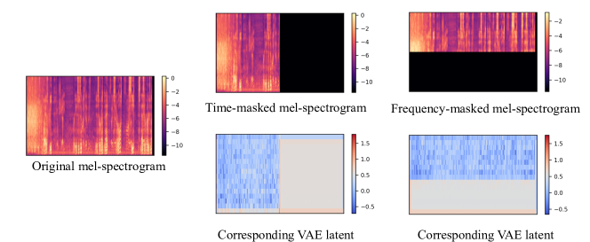
Figure 7: Visualization of the time-frequency-masked spectrogram and their corresponding VAE latent. This figure shows VAE encoder roughly preserves the spatial correspondancy between the spectrogram and the latent.

D Vocoder

In this work, we employ HiFi-GAN (Kong et al., 2020a) as a vocoder, which is widely used for speech waveform generation. It contains two sets of discriminators, a multi-period discriminator, and a multi-scale discriminator, to enhance the perceptual quality. To synthesize the audio waveform, we train it on the AudioSet dataset. For the input samples at the sampling rate of $16,000$Hz, we extract $64$ bands mel-spectrogram. Then we follow the default settings of HiFi-GAN V$1$. The window, FFT, and hop size are set to $1024$, $1024$, and $160$. The $f_{\text{min}}$ and $f_{\text{max}}$ are set as $0$ and $8000$. We use the AdamW optimizer with $0.8$ and $0.99$. The learning rate starts from $2\times 10^{-4}$ and a learning rate decay of $0.999$ is used. We use a batch size of $96$ and train the model with $6$ NVIDIA $3090$ GPUs. We release this pretrained vocoder in our open-source implementation.

E Experiment Details

Data Processing The duration of the audio samples in AudioSet and AudioCaps is $10$ seconds, while it is much longer in FreeSound and BBC SFX datasets. To avoid overusing the data from long audio, which usually have repeated sound, we only use the first thirty seconds of the audio in both the FreeSound and BBC SFX datasets and segment them into ten-second long audio files. Finally, we have in total $3,302,553$ ten-seconds audio samples for model training. It should be noted that even if some datasets, e.g., AudioCaps and BBC SFX, have text captions for the audio, we do not utilize them during the training of LDMs. We only use the audio samples for training. We resample all the datasets into $16$kHz sampling rate and mono format, and all samples are padded to $10$ seconds.

Configuration For each LDM model, we use the compression level $r\texttt{=}4$ as the default setting. Then, we train AudioLDM-S and AudioLDM-L for $0.6$M steps on a single GPU, NVIDIA RTX $3090$, with the batch size of $5$ and $8$, respectively. The learning rate is set as $3\times 10^{-5}$. The AudioLDM-L-Full is trained for $1.5$M steps on one NVIDIA A$100$ with a batch size of $8$. The learning rate is $10^{-5}$. For better performance on AudioCaps, we further fine-tune AudioLDM-L-Full on AudioCaps for $0.25$M steps before evaluation. It should be noted that we limit our batch size because of the scarcity of GPU. However, this potentially restricts the performance of AudioLDM models. In comparison, DiffSound uses $32$ NVIDIA V$100$ GPUs for model training with a batch size of $16$ on each GPU. AudioGen utilizes $64$ A$100$ GPUs with a batch size of $256$.

Human evaluation We construct the dataset for human subjective evaluation with $70$ randomly selected samples where $30$ audios are from AudioCaps, $30$ audios are from AudioSet, and $10$ randomly selected real recordings, which we will refer to as spam cases. Therefore, each model should generate $60$ audio samples given the corresponding text descriptions. We gather the output from models in one folder and anonymize them with random identifiers. An example questionnaire is shown in Table 9. The participant will need to fill in the last two columns for each audio file given the text description. Our final result shows that all the human raters have an average score above $90$ on the spam cases. Hence, their evaluation result is considered reliable.

File name	Text description	Overall impression (1-100)	Relation to the text description (1-100)
random_name_108029.wav	A man talking followed by lights scrapping on a wooden surface	80	90
random_name_108436.wav	Bicycle Music Skateboard Vehicle	70	80
random_name_116883.wav	A power tool drilling as rock music plays	90	95
…	…	…	…

Table 9: Example questionnaire for human evaluation. The participant will need to fill in the last two columns.

F The Effect of Finetuning

Model	Text Data	Use CLAP	Finetuned	FD $\downarrow$	IS $\uparrow$	KL $\downarrow$	FAD $\downarrow$
AudioLDM-S-Full-Roberta	✓	✗	✗	$34.28$	$3.53$	$3.44$	$6.96$
AudioLDM-S-Full-Roberta	✓	✗	✓	$32.13$	$4.02$	$3.25$	$5.89$
AudioLDM-S-Full	✗	✓	✗	$24.13$	$6.68$	$2.36$	$4.94$
AudioLDM-S-Full	✗	✓	✓	$23.47$	$7.57$	$1.98$	$2.32$
AudioLDM-L-Full	✗	✓	✗	$23.51$	$7.11$	$2.19$	$4.19$
AudioLDM-L-Full	✗	✓	✓	$23.31$	$8.13$	$1.59$	$1.96$

Table 10: The comparison between fine-tuned and non-finetuned models on the AudioCaps evaluation set.

Table 10 compares the results obtained with and without fine-tuning on the evaluation set. We observe an improvement in various evaluation metrics, which is expected since the training set of AudioCaps has a distribution that is similar to the evaluation set. However, it is important to note that higher performance on the limited distribution of the evaluation set may not necessarily indicate better performance overall. A model that can generate broader distributions of audio may perform worse on the evaluation set, even though it may have better generalization capabilities. Future work in audio generation can focus on building an evaluation protocal that is more aligned with human perceptions.

G Computation Efficiency Comparison

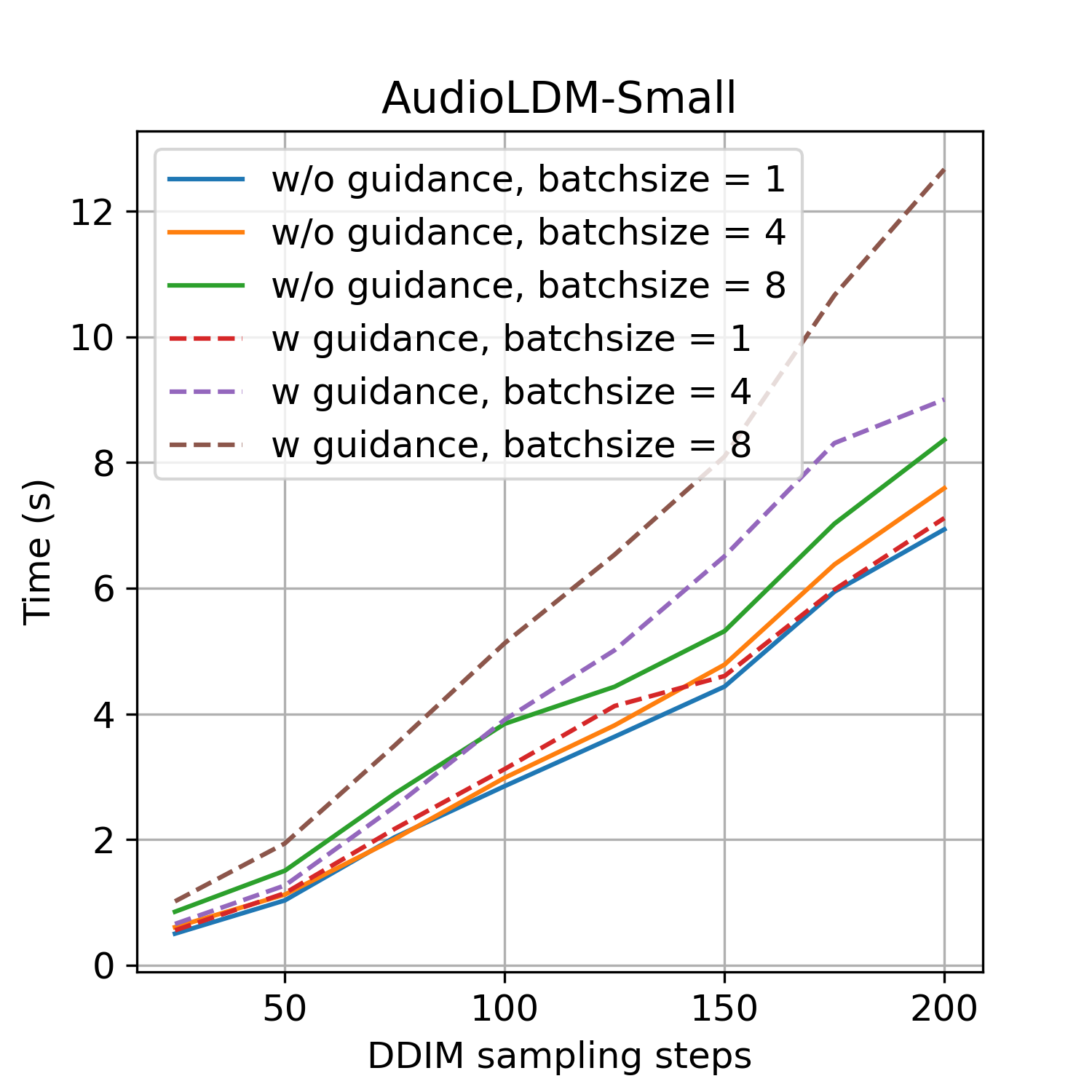
(a) Different batch sizes

(b) Different sampling steps

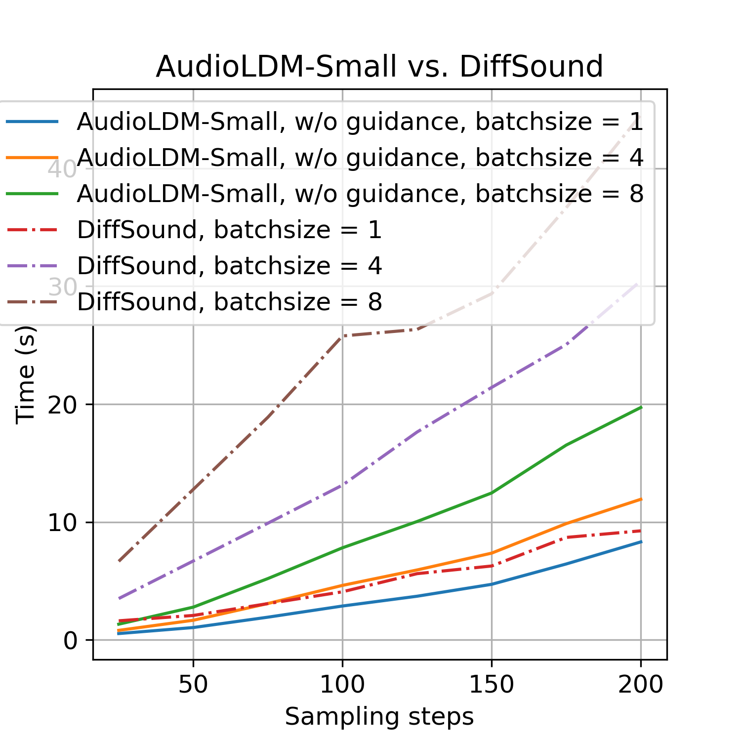
(c) With/Without classifier-free guidance

Figure 8: These three figures show the time cost when generating ten seconds of audio, measured on a single A100 GPU.

As shown in Figure 8(a), AudioLDM-S can generate eight ten-second-long audios within ten seconds without classifier-free guidance. With classifier-free guidance, AudioLDM-Small can generate eight ten-second-long audios with $150$ DDIM steps. Figure 8(c) shows our model is faster than the DiffSound on different batch sizes. Our model can generate eight ten-second-long audios with $20$ seconds while DiffSound needs more than $40$ seconds. Since AudioGen has not been open-sourced yet, we did not perform a speed comparison with AudioGen.

H Limitations

There are several limitations to our study that warrant further investigation in future work. For example, the sampling rate of our model is still insufficient, especially for the generation of music. Exploring higher-fidelity sampling rates such as 32 kHz or 48 kHz could improve the quality of the generated audio. Also, all the modules in AudioLDM are trained separately, which may result in misalignment between different modules. For instance, the latent space learned by VAE may not be optimal for the latent diffusion model. Future work can explore approaches to better align the different modules, such as end-to-end fine-tuning.

The possible negative impact of our method might be the abuse of our technology or released models, e.g., generating fake audio effects to provide misleading information. Moreover, sensitive text content should be restricted in future work to prevent the creation of harmful audio content.

I Demos

Audio Style Transfer

We show three examples of zero-shot audio style transfer with AudioLDM-S, using the developed shallow reverse process (see Equation 10). In Figure 9, we show the transfer from drum beats to ambient music. From left to right, we show the source audio sample drum beats, and the six generated samples guided by text prompt ambient music with different starting points $n_{0}$. Given a smaller $n_{0}$ (i.e., the left part of the figure), the generated sample is similar to drum beats, while when we set $n_{0}=0.8\times N$ for the last sample, the generated sample will be aligned with the text input ambient music. Similarly, we show the source audio trumpt, and the seven generated samples guided by text prompt children singing in Figure 10. We show the source audio sheep vocalization, and the five generated samples guided by text prompt narration, monologue in Figure 11.

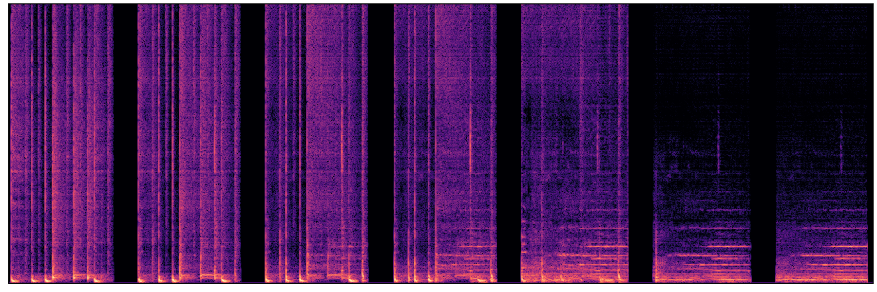
Figure 9: Audio style transfer from drum beats to ambient music.

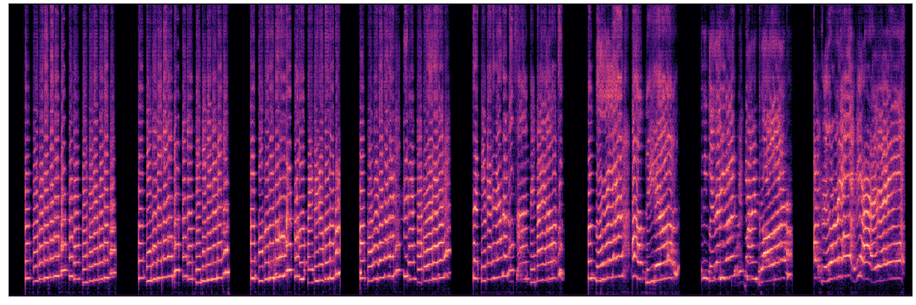
Figure 10: Audio style transfer from trumpet to children singing.

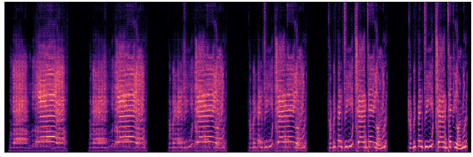
Figure 11: Audio style transfer from sheep vocalization to narration, monologue.

Audio Super-Resolution

In Figure 12, we show four cases of zero-shot audio super-resolution with AudioLDM-S: $1$) violin, $2$) sneezing sound from a woman, $3$) baby crying, and $4$) female speech. The sampling rate of input samples (left) is $8$ kHz, and that of generated samples (middle) and ground-truth samples (right) is $16$ kHz. Our visualization shows we can retain the ground-truth observation in the low-frequency part (below $8$ kHz), while generating the high-frequency missing part (from $8$ kHz to $16$ kHz) with pretrained AudioLDM-S. The generated high-frequency information is consistent with the low-frequency observation.

Figure 12: The examples of zero-shot audio super-resolution with AudioLDM-S.

Audio Inpainting

In Figure 13, we show four samples of zero-shot audio inpainting with AudioLDM-S. The time length of each audio sample is $10$ seconds. In the unprocessed part, we remove the content between $2.5$ and $7.5$ seconds from the ground-truth sample as the input of inpainting. In the inpainting result part, we show the generated samples guided by the same text prompt of the ground-truth sample. In the ground truth part, we show the ground-truth sample for comparison.

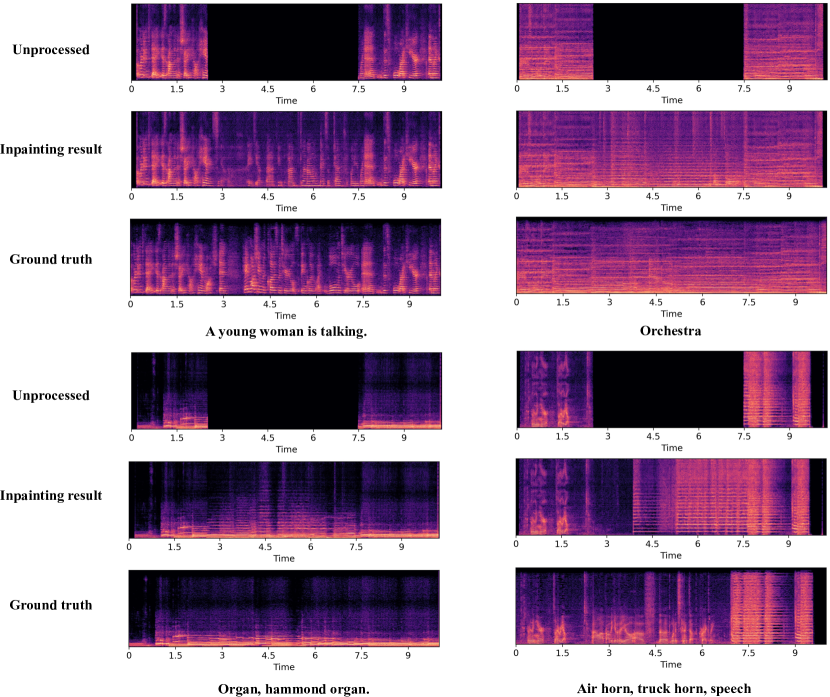
Figure 13: The examples of zero-shot audio inpainting with AudioLDM-S.

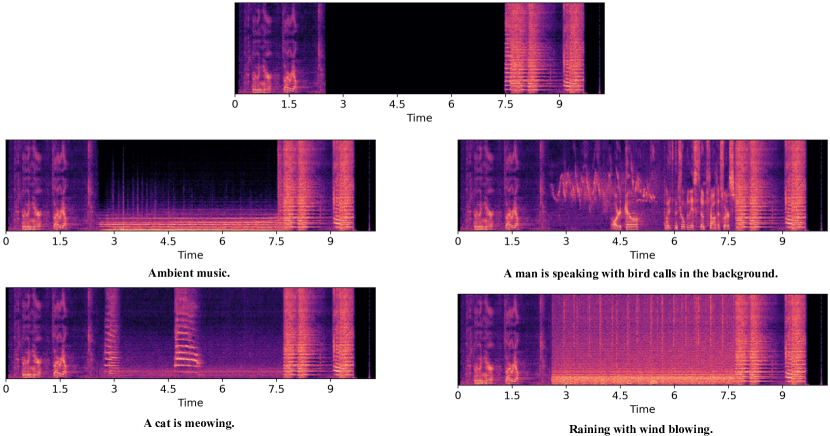
Figure 14: The example of zero-shot audio inpainting with AudioLDM-S given different text prompts.

In Figure 14, we use one sample to demonstrate the audio inpainting guided by different text prompts. Given the observed audio signal shown in the top row, we guide the inpainting process with four different text prompts: $1$) ambient music; $2$) a man is speaking with bird calls in the background; $3$) a cat is meowing; $4$) raining with wind blowing. As can be seen, the observed audio signal is preserved in each generated sample, while the generated content can be controlled by text input.

Environment Control

In Figure 15, we demonstrate that AudioLDM can control the acoustic environment of generated samples with a text description. The four samples are generated with the same random seed, but with different text prompts. Their common text information is “A man is speaking in”, while the specific text information describes the acoustic environment as “a small room”, “a huge room”, “a huge room without background noise”, and “a studio”. These samples show the ability of AudioLDM to capture the fine-grained text description about the acoustic environment, and control the corresponding effects on audio samples, such as reverberation or background noise.

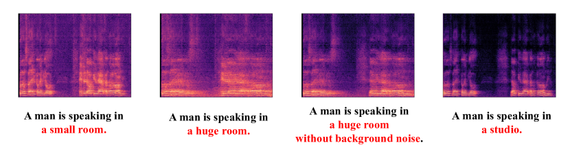
Figure 15: The examples of controlling acoustic environment with AudioLDM-S.

Music Control

In Figure 16, we show the generated music samples when we control the music characteristics with text input. The first sample is generated by “Theme music with bass drum”. Then, we add specific text information “flute”, “fast, flute”, or “flute in the background”, to change the text input. The corresponding variations can be seen in generated mel-spectrograms. We use these samples to demonstrate the ability of AudioLDM to add new musical instruments to music samples, tune the speed of music, and control the foreground-background relations.

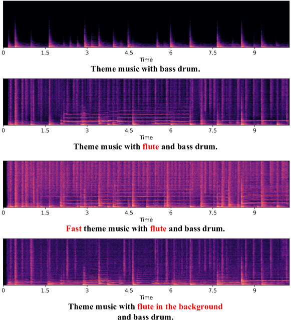
Figure 16: The examples of controlling music characteristics with AudioLDM-S.

Pitch Control

In Figure 17, we show the ability of AudioLDM to control the pitch of generated samples. Pitch is an important characteristic of sound effects, music and speech. Here, we set the common text information as “Sine wave with $\cdots$ pitch”, and input the specific text information “low”, “medium”, and “high”. The text-controlled pitch variation can be seen from the three generated samples.

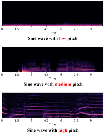
Figure 17: The examples of pitch controlling on generating samples with AudioLDM-S.

Material Control

In Figure 18, we show the ability of AudioLDM to control the materials which generate audio samples. We show four samples generated by the common action “hit” between different materials, e.g., wooden object and wooden environment, or metal object and wooden environment.

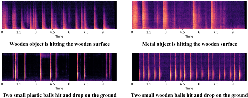
Figure 18: The examples of controlling the materials of generated audio samples with AudioLDM-S.

Temporal Order Control

In Figure 19, we show the ability of AudioLDM to control the temporal order between generated compositional audio signals. When the text description includes multiple sound effects, AudioLDM can generate the audio signals, and the temporal order between them is consistent with the text input.

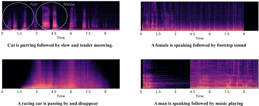
Figure 19: The examples of controlling the temporal order between generated compositional audio samples with AudioLDM-S.

Text-to-Audio Generation

In Figure 20, we show four text-to-audio generation results with AudioLDM-S. They include sound effects in natural environment, human speech, human activity, and sound from objects interaction.

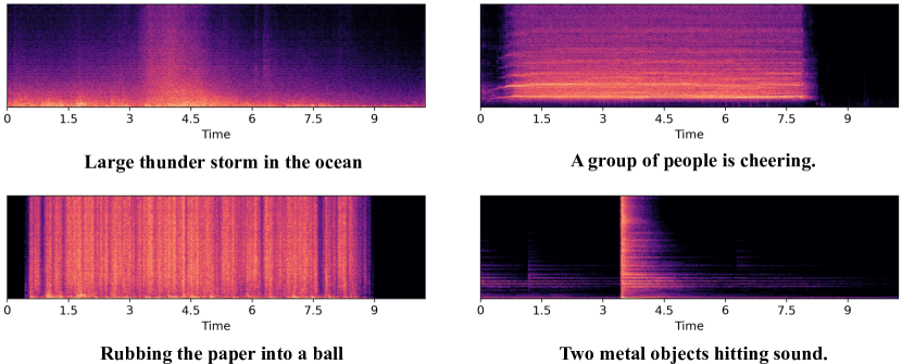
Figure 20: The examples of text-to-audio generation with AudioLDM-S.

Novel Audio Generation

In Figure 21, we show four novel audio samples generated with AudioLDM-S. Their text description is rarely seen, e.g., “A wolf is singing a beautiful song.”. We use them to exhibit the generalization ability of AudioLDM.

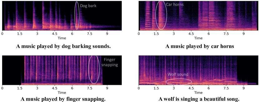
Figure 21: The examples of novel audio generation with AudioLDM-S.

Music Generation

In Figure 22, we show four music samples generated with AudioLDM-S. Here, we are using the labels of AudioSet as text description for music generation, and we are able to specify the music genres of generated samples such as Classical music.

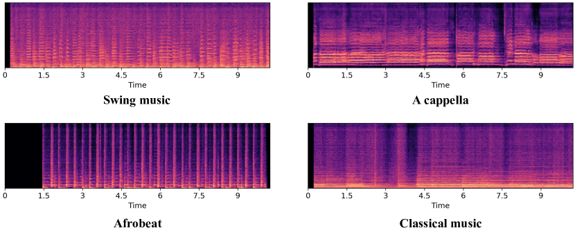
Figure 22: The examples of music generation with AudioLDM-S.

References

- Andresen (1979) Andresen, U. A new way in sound synthesis. In Audio Engineering Society. Audio Engineering Society, 1979.
- Chen et al. (2022a) Chen, K., Du, X., Zhu, B., Ma, Z., Berg-Kirkpatrick, T., and Dubnov, S. HTS-AT: A hierarchical token-semantic audio transformer for sound classification and detection. In IEEE International Conference on Acoustics, Speech and Signal Processing, 2022a.
- Chen et al. (2021) Chen, N., Zhang, Y., Zen, H., Weiss, R., Norouzi, M., and Chan, W. Wavegrad: Estimating gradients for waveform generation. In International Conference on Learning Representations, 2021.
- Chen et al. (2022b) Chen, Z., Tan, X., Wang, K., Pan, S., Mandic, D., He, L., and Zhao, S. Infergrad: Improving diffusion models for vocoder by considering inference in training. In IEEE International Conference on Acoustics, Speech and Signal Processing, 2022b.
- Chen et al. (2022c) Chen, Z., Wu, Y., Leng, Y., Chen, J., Liu, H., Tan, X., Cui, Y., Wang, K., He, L., Zhao, S., Bian, J., and Mandic, D. Resgrad: Residual denoising diffusion probabilistic models for text to speech. arXiv preprint:2212.14518, 2022c.
- Dhariwal & Nichol (2021) Dhariwal, P. and Nichol, A. Diffusion models beat gans on image synthesis. In Conference on Neural Information Processing Systems, 2021.
- Drossos et al. (2020) Drossos, K., Lipping, S., and Virtanen, T. Clotho: an audio captioning dataset. In IEEE International Conference on Acoustics, Speech and Signal Processing, 2020.
- Engel et al. (2020) Engel, J., Hantrakul, L., Gu, C., and Roberts, A. Ddsp: Differentiable digital signal processing. arXiv preprint:2001.04643, 2020.
- Gemmeke et al. (2017) Gemmeke, J. F., Ellis, D. P., Freedman, D., Jansen, A., Lawrence, W., Moore, R. C., Plakal, M., and Ritter, M. AudioSet: An ontology and human-labeled dataset for audio events. In IEEE International Conference on Acoustics, Speech and Signal Processing, pp. 776–780. IEEE, 2017.
- Gong et al. (2021) Gong, Y., Chung, Y.-A., and Glass, J. PSLA: Improving audio tagging with pretraining, sampling, labeling, and aggregation. IEEE/ACM Transactions on Audio, Speech, and Language Processing, 29:3292–3306, 2021.
- Hershey et al. (2017) Hershey, S., Chaudhuri, S., Ellis, D. P., Gemmeke, J. F., Jansen, A., Moore, R. C., Plakal, M., Platt, D., Saurous, R. A., Seybold, B., et al. CNN architectures for large-scale audio classification. In 2017 IEEE International Conference on Acoustics, Speech and Signal Processing, pp. 131–135. IEEE, 2017.
- Ho & Salimans (2021) Ho, J. and Salimans, T. Classifier-free diffusion guidance. In NeurIPS Workshop on Deep Generative Models and Downstream Applications, 2021.
- Ho et al. (2020) Ho, J., Jain, A., and Abbeel, P. Denoising diffusion probabilistic models. In Conference on Neural Information Processing Systems, 2020.
- Ho et al. (2022) Ho, J., Chan, W., Saharia, C., Whang, J., Gao, R., Gritsenko, A., Kingma, D. P., Poole, B., Norouzi, M., Fleet, D. J., and Salimans, T. Imagen video: High definition video generation with diffusion models. arXiv preprint:2210.02303, 2022.
- Isola et al. (2017) Isola, P., Zhu, J.-Y., Zhou, T., and Efros, A. A. Image-to-image translation with conditional adversarial networks. In Proceedings of the IEEE/CVF Conference on Computer Vision and Pattern Recognition, pp. 1125–1134, 2017.
- Karplus & Strong (1983) Karplus, K. and Strong, A. Digital synthesis of plucked-string and drum timbres. Computer Music Journal, 7(2):43–55, 1983.
- Kilgour et al. (2019) Kilgour, K., Zuluaga, M., Roblek, D., and Sharifi, M. Fréchet audio distance: A reference-free metric for evaluating music enhancement algorithms. In INTERSPEECH, pp. 2350–2354, 2019.
- Kim et al. (2019) Kim, C. D., Kim, B., Lee, H., and Kim, G. Audiocaps: Generating captions for audios in the wild. In Proceedings of the 2019 Conference of the North American Chapter of the Association for Computational Linguistics: Human Language Technologies, pp. 119–132, 2019.
- Kingma & Ba (2014) Kingma, D. P. and Ba, J. Adam: A method for stochastic optimization. arXiv preprint:1412.6980, 2014.
- Kingma & Welling (2013) Kingma, D. P. and Welling, M. Auto-encoding variational bayes. arXiv preprint:1312.6114, 2013.
- Kong et al. (2020a) Kong, J., Kim, J., and Bae, J. Hifi-gan: Generative adversarial networks for efficient and high fidelity speech synthesis. Advances in Neural Information Processing Systems, 33:17022–17033, 2020a.
- Kong et al. (2020b) Kong, Q., Cao, Y., Iqbal, T., Wang, Y., Wang, W., and Plumbley, M. D. PANNs: Large-scale pretrained audio neural networks for audio pattern recognition. IEEE/ACM Transactions on Audio, Speech, and Language Processing, 28:2880–2894, 2020b.
- Kong et al. (2021a) Kong, Q., Cao, Y., Liu, H., Choi, K., and Wang, Y. Decoupling magnitude and phase estimation with deep resunet for music source separation. arXiv preprint:2109.05418, 2021a.
- Kong et al. (2021b) Kong, Z., Ping, W., Huang, J., Zhao, K., and Catanzaro, B. Diffwave: A versatile diffusion model for audio synthesis. In International Conference on Learning Representations, 2021b.
- Kreuk et al. (2022) Kreuk, F., Synnaeve, G., Polyak, A., Singer, U., Défossez, A., Copet, J., Parikh, D., Taigman, Y., and Adi, Y. Audiogen: Textually guided audio generation. arXiv preprint:2209.15352, 2022.
- Kuleshov et al. (2017) Kuleshov, V., Enam, S. Z., and Ermon, S. Audio super resolution using neural networks. arXiv:1708.00853, 2017.
- Lam et al. (2022) Lam, M., Wang, J., Huang, R., Su, D., and Yu, D. Bilateral denoising diffusion models. In International Conference on Learning Representations, 2022.
- Lee et al. (2022) Lee, S., Kim, H., Shin, C., Tan, X., Liu, C., Meng, Q., Qin, T., Chen, W., Yoon, S., and Liu, T. Priorgrad: Improving conditional denoising diffusion models with data-driven adaptive prior. In International Conference on Learning Representations, 2022.
- Leng et al. (2022) Leng, Y., Chen, Z., Guo, J., Liu, H., Chen, J., Tan, X., Mandic, D., He, L., Li, X.-Y., Qin, T., et al. Binauralgrad: A two-stage conditional diffusion probabilistic model for binaural audio synthesis. arXiv preprint:2205.14807, 2022.
- Liu et al. (2021a) Liu, H., Kong, Q., Tian, Q., Zhao, Y., Wang, D., Huang, C., and Wang, Y. Voicefixer: Toward general speech restoration with neural vocoder. arXiv preprint:2109.13731, 2021a.
- Liu et al. (2022a) Liu, H., Choi, W., Liu, X., Kong, Q., Tian, Q., and Wang, D. Neural vocoder is all you need for speech super-resolution. arXiv preprint:2203.14941, 2022a.
- Liu et al. (2022b) Liu, H., Kong, Q., Liu, X., Mei, X., Wang, W., and Plumbley, M. D. Ontology-aware learning and evaluation for audio tagging. arXiv preprint:2211.12195, 2022b.
- Liu et al. (2022c) Liu, H., Liu, X., Kong, Q., Wang, W., and Plumbley, M. D. Learning the spectrogram temporal resolution for audio classification. arXiv preprint:2210.01719, 2022c.
- Liu et al. (2022d) Liu, N., Li, S., Du, Y., Torralba, A., and Tenenbaum, J. B. Compositional visual generation with composable diffusion models. In European Conference on Computer Vision, 2022d.
- Liu et al. (2021b) Liu, X., Iqbal, T., Zhao, J., Huang, Q., Plumbley, M. D., and Wang, W. Conditional sound generation using neural discrete time-frequency representation learning. In IEEE International Workshop on Machine Learning for Signal Processing, pp. 1–6. IEEE, 2021b.
- Liu et al. (2022e) Liu, X., Liu, H., Kong, Q., Mei, X., Plumbley, M. D., and Wang, W. Simple pooling front-ends for efficient audio classification. arXiv preprint:2210.00943, 2022e.
- Liu et al. (2022f) Liu, X., Liu, H., Kong, Q., Mei, X., Zhao, J., Huang, Q., Plumbley, M. D., and Wang, W. Separate what you describe: language-queried audio source separation. arXiv preprint:2203.15147, 2022f.
- Liu et al. (2019) Liu, Y., Ott, M., Goyal, N., Du, J., Joshi, M., Chen, D., Levy, O., Lewis, M., Zettlemoyer, L., and Stoyanov, V. Roberta: A robustly optimized BERT pretraining approach. arXiv preprint:1907.11692, 2019.
- Nichol & Dhariwal (2021) Nichol, A. and Dhariwal, P. Improved denoising diffusion probabilistic models. In International Conference on Machine Learning, 2021.
- Nichol et al. (2021) Nichol, A., Dhariwal, P., Ramesh, A., Shyam, P., Mishkin, P., McGrew, B., Sutskever, I., and Chen, M. Glide: Towards photorealistic image generation and editing with text-guided diffusion models. arXiv preprint:2112.10741, 2021.
- Oord et al. (2016) Oord, A. v. d., Dieleman, S., Zen, H., Simonyan, K., Vinyals, O., Graves, A., Kalchbrenner, N., Senior, A., and Kavukcuoglu, K. WaveNet: A generative model for raw audio. arXiv preprint:1609.03499, 2016.
- Pascual et al. (2022) Pascual, S., Bhattacharya, G., Yeh, C., Pons, J., and Serrà, J. Full-band general audio synthesis with score-based diffusion. arXiv preprint:2210.14661, 2022.
- Perez et al. (2018) Perez, E., Strub, F., De Vries, H., Dumoulin, V., and Courville, A. Film: Visual reasoning with a general conditioning layer. In Proceedings of the AAAI Conference on Artificial Intelligence, volume 32, 2018.
- Popov et al. (2021) Popov, V., Vovk, I., Gogoryan, V., Sadekova, T., and Kudinov, M. Grad-tts: A diffusion probabilistic model for text-to-speech. In International Conference on Machine Learning, 2021.
- Radford et al. (2021) Radford, A., Kim, J. W., Hallacy, C., Ramesh, A., Goh, G., Agarwal, S., Sastry, G., Askell, A., Mishkin, P., Clark, J., Krueger, G., and Sutskever, I. Learning transferable visual models from natural language supervision. In International Conference on Machine Learning, 2021.
- Raffel et al. (2020) Raffel, C., Shazeer, N., Roberts, A., Lee, K., Narang, S., Matena, M., Zhou, Y., Li, W., and Liu, P. J. Exploring the limits of transfer learning with a unified text-to-text transformer. Journal of Machine Learning Research, 2020.
- Ramesh et al. (2022) Ramesh, A., Dhariwal, P., Nichol, A., Chu, C., and Chen, M. Hierarchical text-conditional image generation with clip latents. arXiv preprint:2204.06125, 2022.
- Rombach et al. (2022) Rombach, R., Blattmann, A., Lorenz, D., Esser, P., and Ommer, B. High-resolution image synthesis with latent diffusion models. In Proceedings of the IEEE/CVF Conference on Computer Vision and Pattern Recognition, pp. 10684–10695, 2022.
- Saharia et al. (2021) Saharia, C., Ho, J., Chan, W., Salimans, T., Fleet, D. J., and Norouzi, M. Image super-resolution via iterative refinement. arXiv preprint:2104.07636, 2021.
- Saharia et al. (2022) Saharia, C., Chan, W., Saxena, S., Li, L., Whang, J., Denton, E., Ghasemipour, S. K. S., Ayan, B. K., Mahdavi, S. S., Lopes, R. G., Salimans, T., Ho, J., Fleet, D. J., and Norouzi, M. Photorealistic text-to-image diffusion models with deep language understanding. arXiv preprint:2205.11487, 2022.
- Salamon et al. (2014) Salamon, J., Jacoby, C., and Bello, J. P. A dataset and taxonomy for urban sound research. In Proceedings of the 22nd ACM international conference on Multimedia, pp. 1041–1044, 2014.
- Schuhmann et al. (2021) Schuhmann, C., Vencu, R., Beaumont, R., Kaczmarczyk, R., Mullis, C., Katta, A., Coombes, T., Jitsev, J., and Komatsuzaki, A. Laion-400m: Open dataset of clip-filtered 400 million image-text pairs. arXiv preprint:2111.02114, 2021.
- Singer et al. (2022) Singer, U., Polyak, A., Hayes, T., Yin, X., An, J., Zhang, S., Hu, Q., Yang, H., Ashual, O., Gafni, O., Parikh, D., Gupta, S., and Taigman, Y. Make-a-video: Text-to-video generation without text-video data. arXiv preprint:2209.14792, 2022.
- Sinha et al. (2021) Sinha, A., Song, J., Meng, C., and Ermon, S. D2c: Diffusion-decoding models for few-shot conditional generation. In Conference on Neural Information Processing Systems, 2021.
- Song et al. (2020) Song, J., Meng, C., and Ermon, S. Denoising diffusion implicit models. arXiv preprint:2010.02502, 2020.
- Song et al. (2021) Song, Y., Sohl-Dickstein, J., Kingma, D., Kumar, A., Ermon, S., and Poole, B. Score-based generative modeling through stochastic differential equations. In International Conference on Learning Representations, 2021.
- Tan et al. (2022) Tan, X., Chen, J., Liu, H., Cong, J., Zhang, C., Liu, Y., Wang, X., Leng, Y., Yi, Y., He, L., et al. NaturalSpeech: End-to-end text to speech synthesis with human-level quality. arXiv preprint:2205.04421, 2022.
- Vahdat et al. (2021) Vahdat, A., Kreis, K., and Kautz, J. Lsgm: Score-based generative modeling in latent space. In Conference on Neural Information Processing Systems, 2021.
- Wang & Wang (2021) Wang, H. and Wang, D. Towards robust speech super-resolution. IEEE/ACM Transactions on Audio, Speech, and Language Processing, 29:2058–2066, 2021.
- Wu et al. (2022) Wu, Y., Chen, K., Zhang, T., Hui, Y., Berg-Kirkpatrick, T., and Dubnov, S. Large-scale contrastive language-audio pretraining with feature fusion and keyword-to-caption augmentation. arXiv preprint:2211:06687, 2022.
- Yamagishi et al. (2019) Yamagishi, J., Veaux, C., MacDonald, K., et al. CSTR VCTK corpus: English multi-speaker corpus for cstr voice cloning toolkit. 2019.
- Yang et al. (2022) Yang, D., Yu, J., Wang, H., Wang, W., Weng, C., Zou, Y., and Yu, D. Diffsound: Discrete diffusion model for text-to-sound generation. arXiv preprint:2207.09983, 2022.
- Żelaszczyk & Mańdziuk (2022) Żelaszczyk, M. and Mańdziuk, J. Audio-to-image cross-modal generation. In International Joint Conference on Neural Networks, pp. 1–8. IEEE, 2022.