G-fractional diffusion on bounded domains in $\mathbb{R}^{d}$

Abstract.

In this paper we study $g$-fractional diffusion on bounded domains in $\mathbb{R}^{d}$ with absorbing boundary conditions. A new general and explicit representation of the solution is obtained. We study the first-passage time distribution, showing the dependence on the particular choice of the function $g$. Then, we specialize the analysis to the interesting case of a rectangular domain. Finally, we briefly discuss the connection of this general theory with the physical application to the so-called fractional Dodson diffusion model, recently discussed in the literature.

1. Introduction

Time-fractional diffusion processes are widely studied in the literature for their relation to continuous-time random walks (see, e.g., [12]) and for pervasive applications in various fields, from applied physics to pure mathematics and probability (see, for example, the recent monograph [8] and references therein). More recently, $g$-fractional diffusive equations based on the application of fractional derivatives with respect to another function (also named, in the mathematical literature, $\Psi$-fractional derivatives) have gained greater interest. In particular, in a series of interesting papers [13, 14, 15], the authors discussed the relevance of this approach for physical models of anomalous diffusion. In the mathematical literature, starting from the paper by Almeida [1], many papers have been devoted to the analysis of fractional differential equations with respect to another function and this is a developing field, as it allows nontrivial generalizations of classical equations involving Caputo derivatives.

In [2] we have considered the one-dimensional $g$-fractional diffusion equation with absorbing boundary conditions. An interesting outcome of the analysis developed in [2] is that the explicit solution can be found and particular choices of the $g$-function leads to a finite mean first-passage time (MFPT), differently from the time-fractional diffusion in bounded domain involving the classical Caputo derivative (which is the special case $g(t)=t$). In this paper we consider, for the first time, the $g$-fractional diffusion in $d$-dimensional bounded domains with absorbing boundary conditions. We obtain the explicit representation of the solution for the Dirichlet problem in $\mathbb{R}^{d}$, which can be applied to several particular diffusive models in bounded domains. We emphasize that the main difference with the more particular (and simple) one-dimensional case previously treated in [2] lies in the broad generality of the main results presented here, which can be used for realistic diffusive models in higher dimensions. We then study the first-passage time distribution (FPTD), discussing the condition for a finite MFPT.
As a first application of the general results obtained here, we consider the special and interesting case of $g$-fractional diffusion in rectangular domains. We recall that fractional diffusions in multidimensional rectangular domains have been the subject of recent interest in the mathematical literature (see, for example, [18]).
In the final section, we investigate the case of fractional Dodson equation, recently introduced in [9]. This is an interesting heuristic model of fractional diffusion that includes, at the same time, memory effects and the particular exponential time-dependence of the diffusion coefficient. The peculiarity of this model relies on the fact that the corresponding $g$-function is upper bounded, resulting in the existence of stationary solutions, finite values of the asymptotic survival probability and, therefore, undefined MFPT.

2. G-fractional diffusion in bounded domains

We consider a $g$-fractional diffusion process on a bounded domain $\Omega$ in $\mathbb{R}^{d}$:

(2.1) $$\left(\frac{{}^{C}\partial_{g}^{\alpha}u}{\partial t^{\alpha}}\right)({\bf r},t)=D\nabla^{2}u({\bf r},t),$$

where ${\bf r}=\{x_{1},...,x_{d}\}$, $\nabla^{2}=\sum_{i=1}^{d}\frac{\partial^{2}}{\partial x_{i}^{2}}$ is the Laplacian in dimension $d$, $D$ is the generalized diffusion constant and the Caputo-type $g$-fractional derivative of order $\alpha\in(0,1)$ is defined as

(2.2) $$\left(\frac{{}^{C}\partial_{g}^{\alpha}u}{\partial t^{\alpha}}\right)({\bf r},t):=\frac{1}{\Gamma(1-\alpha)}\int_{0}^{t}(g(t)-g(\tau))^{-\alpha}\ \frac{\partial u}{\partial\tau}({\bf r},\tau)d\tau,$$

where $g(t)$ is a deterministic function such that $g(0)=0$ and $g^{\prime}(t)>0$ for $t>0$, where we denote by $g^{\prime}=dg/dt$ the first order time derivative. We consider generic initial condition

(2.3) $$u({\bf r},0)=u_{0}({\bf r}),$$

and absorbing (Dirichlet) boundary conditions

(2.4) $$u({\bf r},t)=0,\hskip 28.45274pt{\bf r}\in\partial\Omega.$$

Solutions can be found by the method of separation of variables, i.e.

$$u({\bf r},t)=X({\bf r})T(t).$$

We have to solve the two equations

(2.5) $$\frac{{}^{C}d_{g}^{\alpha}T(t)}{dt^{\alpha}}=-\lambda DT(t),$$

and

(2.6) $$\nabla^{2}X({\bf r})=-\lambda X({\bf r}).$$

The solution of (2.5) is

(2.7) $$T(t)=T(0)\ E_{\alpha}(-\lambda Dg(t)^{\alpha}),$$

where $E_{\alpha}(\cdot)$ denotes the one-parameter Mittag-Leffler function [10]

(2.8) $$E_{\alpha}(x)=\sum_{k=0}^{\infty}\frac{x^{k}}{\Gamma(\alpha k+1)}.$$

The eigenvalue problem (2.6) – with boundary conditions (2.4) – is solved by an infinite sequence of pairs $(\lambda_{n},\phi_{n})$, with $n\geq 1$ ($\lambda_{1}<\lambda_{2}<...$) and $\phi_{n}({\bf r})$ is a sequence of functions that form a complete orthonormal set in $L^{2}(\Omega)$ [11, 16, 17].
The solution of the $g$-fractional diffusive equation (2.1) can then be expressed as

(2.9) $$u({\bf r},t)=\sum_{n=1}^{\infty}u_{0,n}\ \phi_{n}({\bf r})\ E_{\alpha}(-\lambda_{n}Dg(t)^{\alpha}),$$

where

(2.10) $$u_{0,n}=\int_{\Omega}d{\bf r}\ \phi_{n}({\bf r})\ u_{0}({\bf r}).$$

3. first-passage times

We study here first-passage problems. The FPTD $\varphi(t)$ is defined by

(3.1) $$\varphi(t)=-\frac{d{\mathbb{P}}}{dt}(t),$$

where ${\mathbb{P}}(t)$ is the survival probability, i.e. the probability that a particle has not been absorbed until time $t$

(3.2) $${\mathbb{P}}(t)=\int_{\Omega}d{\bf r}\ u({\bf r},t).$$

We are assuming here that the survival probability goes to zero for $t\to\infty$, i.e., the particle will surely be absorbed during the entire process. This corresponds to consider functions $g(t)$ such that $\lim_{t\to\infty}g(t)=+\infty$. In the last section, treating the fractional Dodson diffusion, we will discuss the main consequences of relaxing such an assumption.
The MFPT $\tau$ is the first moment of (3.1)

(3.3) $$\tau=\int_{0}^{\infty}dt\ t\ \varphi(t).$$

By using (2.9), (3.1) and (3.2), we can then express the FPTD for $g$-fractional diffusion processes as

(3.4) $$\varphi(t)=-\sum_{n=1}^{\infty}u_{0,n}\ \Phi_{n}\ \frac{d}{dt}E_{\alpha}(-\lambda_{n}Dg(t)^{\alpha}),$$

where

(3.5) $$\Phi_{n}=\int_{\Omega}d{\bf r}\ \phi_{n}({\bf r}).$$

By using the property [10]

(3.6) $$E_{\alpha,\alpha}(-x)=-\alpha\frac{d}{dx}E_{\alpha}(-x),$$

where we have introduced the two-parameters Mittag-Leffler function

(3.7) $$E_{\alpha,\beta}(x)=\sum_{k=0}^{\infty}\frac{x^{k}}{\Gamma(\alpha k+\beta)},$$

we finally arrive at the expression for the FPTD

(3.8) $$\varphi(t)=Dg^{\prime}(t)g(t)^{\alpha-1}\sum_{n=1}^{\infty}\lambda_{n}u_{0,n}\ \Phi_{n}\ E_{\alpha,\alpha}(-\lambda_{n}Dg(t)^{\alpha}).$$

It is interesting to show the long time behavior of $\varphi(t)$. By using the asymptotic expansion of the Mittag-Leffler function for $|z|\to\infty$ and $\Re(z)<0$ (see [10], p. 75)

(3.9) $$E_{\alpha,\alpha}(z)=-\frac{z^{-2}}{\Gamma(-\alpha)}+O(|z|^{-3}),$$

we have that the asymptotic behavior of (3.8) is

(3.10) $$\varphi(t)\sim-\frac{g^{\prime}(t)g(t)^{-(\alpha+1)}}{D\Gamma(-\alpha)}\sum_{n=1}^{\infty}\frac{u_{0,n}\ \Phi_{n}}{\lambda_{n}},\hskip 36.98866ptt\to\infty.$$

It is worth noting that the above asymptotic form allows the MFPT (3.3) to be finite only for those functions $g(t)$ satisfying $\lim_{t\to\infty}t^{2}g^{\prime}g^{-\alpha-1}=0$, regardless of boundary shape. In other words, finite MFPTs are obtained if $g(t)$ grows asymptotically faster than $t^{1/\alpha}$, similarly to the one-dimensional case [2].

4. Rectangular domains

We specialize here to the case of rectangle-like domains in ${\mathbb{R}}^{d}$, $\Omega=[0,L_{1}]\times\dots\times[0,L_{d}]$. Variable separation allows the eigenfunctions to be written as (by using the multiple index $n=\{n_{1},...,n_{d}\}$)

(4.1) $$\phi_{n}({\bf r})=\prod_{i=1}^{d}\phi_{n_{i}}^{(i)}(x_{i}),$$

and the eigenvalues as

(4.2) $$\lambda_{n}=\sum_{i=1}^{d}\lambda_{n_{i}}^{(i)}.$$

Considering absorbing boundary conditions (2.4) we have [11, 17]

(4.3) $$\phi_{n_{i}}^{(i)}(x) = (2/L_{i})^{1/2}\ \sin{(\pi n_{i}x/L_{i})},$$

(4.4) $$\lambda_{n_{i}}^{(i)} = \pi^{2}n_{i}^{2}/L_{i}^{2},$$

with $i=1,...,d$ and $n_{i}\geq 1$. Inserting in (2.9) we obtain the solution of the $g$-fractional diffusion equation in rectangular domains with generic initial conditions

(4.5) $$u({\bf r},t)=\sum_{n=1}^{\infty}u_{0,n}\left[\prod_{i=1}^{d}\sqrt{\frac{2}{L_{i}}}\sin{\left(\frac{\pi n_{i}x_{i}}{L_{i}}\right)}\right]\ E_{\alpha}\left(-\lambda_{n}Dg(t)^{\alpha}\right),$$

where $\lambda_{n}$ are given by (4.2). In the following we consider $\delta$-peaked initial conditions

(4.6) $$u_{0}({\bf r})=\delta({\bf r}-{\bf r}_{0}),$$

where ${\bf r}_{0}=\{x_{1,0},...,x_{d,0}\}$. We have, from (2.10),

(4.7) $$u_{0,n}=\prod_{i=1}^{d}\phi_{n_{i}}^{(i)}(x_{i,0})=\prod_{i=1}^{d}\sqrt{\frac{2}{L_{i}}}\sin{\left(\frac{\pi n_{i}x_{i,0}}{L_{i}}\right)},$$

and the solution (4.5) reads

(4.8) $$u({\bf r},t)=\sum_{n=1}^{\infty}\left[\prod_{i=1}^{d}\frac{2}{L_{i}}\sin{\left(\frac{\pi n_{i}x_{i,0}}{L_{i}}\right)}\sin{\left(\frac{\pi n_{i}x_{i}}{L_{i}}\right)}\right]\ E_{\alpha}\left(-\lambda_{n}Dg(t)^{\alpha}\right).$$

We now turn to analyze the FPTD (3.8). We first note that the terms $\Phi_{n}$ (3.5) can be written as

(4.9) $$\Phi_{n}=\prod_{i=1}^{d}\Phi_{n_{i}}^{(i)},$$

where

(4.10) $$\Phi_{n_{i}}^{(i)} = \int_{0}^{L_{i}}dx\ \phi_{n_{i}}^{(i)}(x)=\sqrt{\frac{2}{L_{i}}}\int_{0}^{L_{i}}dx\ \sin{(\pi n_{i}x/L_{i})}$$

$$= \frac{2\sqrt{2L_{i}}}{\pi n_{i}},\quad\quad\mbox{if $n_{i}$ is odd},$$

and null otherwise. We can finally express the FPTD as

(4.11) $$\varphi(t)=\frac{2^{2d}Dg^{\prime}(t)g(t)^{\alpha-1}}{\pi^{d}}\sum_{n=0}^{\infty}\lambda_{2n+1}\left(\prod_{i=1}^{d}\frac{\sin{(\pi(2n_{i}+1)x_{i,0}/L_{i})}}{2n_{i}+1}\right)\ E_{\alpha,\alpha}(-\lambda_{2n+1}Dg(t)^{\alpha}),$$

where $\lambda_{2n+1}=\sum_{i=1}^{d}\pi^{2}(2n_{i}+1)^{2}/L_{i}^{2}$. We note that for $d=1$ the above expression reduces to that obtained in [2] for the one-dimensional case.

As an example, Figure 1 shows the typical behavior of FPTDs at different values of the fractional order $\alpha$. The curves shown are obtained by numerical evaluation of (4.11) and correspond to the Erdérlyi-Kober derivative $g(t)=t^{\beta}$, with $\beta=2$, in a two-dimensional square box with absorbing boundaries. It is evident the power-law decay at long time, affecting the existence of finite MFPTs – see (3.10) and the discussion at the end of the previous section.

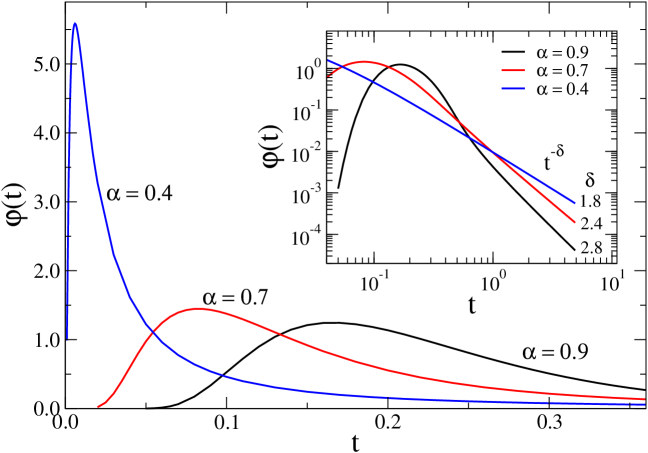
Figure 1. Example of first-passage time distributions at different fractional derivative order $\alpha$ for a particular choice of the $g$-function, $g(t)=t^{2}$ (Erdérlyi-Kober derivative). Inset: the same as in the main panel in logarithmic scale, in order to highlight the long time behavior $t^{-\delta}$. Only the cases for which $\delta=1+2\alpha>2$ correspond to finite values of the MFPT (see (3.10) and subsequent discussion). The curves are obtained by numerical evaluation of the expression (4.11), considering a square box ($d=2$) of size $L=1$ and setting $D=1$, $x_{1,0}=x_{2,0}=L/2$, and $g(t)=t^{2}$.

5. The fractional Dodson diffusion

The Dodson diffusion equation arises in the context of cooling processes in geology [7] and it takes the form (see e.g. [6], pag.104-105)

(5.1) $$\frac{\partial u}{\partial t}=D_{0}\,\exp(-\beta t)\,\frac{\partial^{2}u}{\partial x^{2}},$$

where $1/\beta$ is the so called relaxation time. This is an interesting model where the diffusivity coefficient is time-dependent and, more precisely, it is an exponentially decreasing function of time. As we will see, this slowing down of dynamics generates finite stationary solutions, with important consequences on first-passage processes.

In the recent paper [9], a new generalization of the Dodson diffusion equation was suggested in view of the relevance of the fractional approach for diffusive models with memory effects. In this paper, the fractional Dodson equation is essentially a $g$-fractional diffusion with

(5.2) $$g(t)=\frac{1-e^{-\beta t}}{\beta}.$$

This means that the time-fractional operator appearing in the evolution equation is given by

(5.3) $${}^{C}\left(e^{\beta t}\,\frac{\partial}{\partial t}\right)^{\alpha}u(x,t)=\frac{1}{\Gamma(1-\alpha)}\int_{0}^{t}\left(\frac{e^{-\beta\tau}-e^{-\beta t}}{\beta}\right)^{-\alpha}\,\frac{\partial u}{\partial\tau}\,d\tau,$$

where we used the notation of [9] to underline that this $g$-fractional derivative physically corresponds to an operator that includes the time-dependence of the diffusivity and the memory effects. Moreover, for $\alpha=1$ we recover the classical equation. This is an exploratory generalization of the Dodson diffusion and a concrete potential application of the $g$-fractional approach to diffusive models.
We note that the $g(t)$ (5.2) is a bounded function, as $\lim_{t\to\infty}g(t)=1/\beta$. Having this in mind, we can apply some of the results obtained in the previous sections to the present case of fractional Dodson diffusion in bounded domains with absorbing boundary conditions. We recall that in [9], the authors derived the fundamental solution of the fractional Dodson equation in the one-dimensional case, while the diffusive problem in a bounded domain and in higher dimensions has not been considered before in the literature.
Let us consider the $d$-dimensional fractional Dodson equation

(5.4) $${}^{C}\left(e^{\beta t}\frac{\partial}{\partial t}\right)^{\alpha}u({\bf r},t)=D\nabla^{2}u({\bf r},t),$$

under the initial condition

(5.5) $$u({\bf r},0)=u_{0}({\bf r}),$$

and absorbing boundary conditions

(5.6) $$u({\bf r},t)=0,\hskip 28.45274pt{\bf r}\in\partial\Omega.$$

Then, using the results obtained in the previous sections, we have that the solution can be expressed as

(5.7) $$u({\bf r},t)=\sum_{n=1}^{\infty}u_{0,n}\ \phi_{n}({\bf r})\ E_{\alpha}\bigg{(}-\lambda_{n}D\left(\frac{1-e^{-\beta t}}{\beta}\right)^{\alpha}\bigg{)},$$

where

(5.8) $$u_{0,n}=\int_{\Omega}d{\bf r}\ \phi_{n}({\bf r})\ u_{0}({\bf r}).$$

Thus, the upper bounded $g(t)$ implies the existence of a stationary solution $u_{st.}$:

(5.9) $$u_{st.}({\bf r})=\lim_{t\to\infty}u({\bf r},t)=\sum_{n=1}^{\infty}u_{0,n}\ \phi_{n}({\bf r})\ E_{\alpha}(-\lambda_{n}D\beta^{-\alpha}).$$

We then conclude that the survival probability has a finite asymptotic value

(5.10) $${\mathbb{P}}_{\infty}=\int_{\Omega}d{\bf r}\ u_{st.}({\bf r}),$$

which means that there is a finite probability that the particle will never be absorbed at the boundaries, resulting in a divergent MFPT. This is a general result valid whenever the $g$-function has a finite asymptotic limit, corresponding to a slowing dynamics ending in a “frozen” particle distribution.

6. Conclusions

In this paper we have considered the $g$-fractional diffusion in $\mathbb{R}^{d}$ with absorbing (Dirichlet) boundary conditions. This generalizes the previous one-dimensional study [2] to the $d$-dimensional case. We show that it is possible to find the explicit representation of the solution for a generic $g$-function and bounded domain $\Omega$ in $\mathbb{R}^{d}$. This is the first general treatment of $g$-fractional diffusion in generic $d$ dimension and we obtain a general representation that can be used in realistic models, beyond the one-dimensional analysis developed in the previous literature. We have then analyzed the FPTD and its dependence on the particular choice of the function $g$, leading to a nontrivial generalization of the classical Caputo-fractional diffusion in a bounded domain. We have considered the interesting case of the rectangular domain, obtaining the exact form of the solution. Finally, we have devoted a section to a physical application related to the Dodson diffusion equation recently considered in [9]. In previous research on this topic, the authors obtained the fundamental solution in the one-dimensional case, while here we derive the solution of the Dirichlet problem in higher dimensions. This allows us to discuss the effects of choosing a bounded $g$-function, resulting in a finite asymptotic survival probability and undefined MFPT.

In conclusion, we have demonstrated the nontrivial role of the $g$-function on diffusive behavior in $d$-dimensional domains and its influence on the shape of FPTDs and the existence of finite MFPTs. It would be interesting to extend the analysis to domains of different shapes (such as spherical or cylindrical) and consider different boundary conditions, such as, for example, partial absorption [3, 4] with, possibly, time-dependent rates (see, for example, [5] and references therein) , in order to study the combined effects of fractional diffusion and boundary properties on first-passage processes.

References

- [1] Almeida, R. (2017). A Caputo fractional derivative of a function with respect to another function. Communications in Nonlinear Science and Numerical Simulation, 44, 460-481.
- [2] Angelani, L., Garra, R. (2023). -fractional diffusion models in bounded domains. Phys. Rev. E 107, 014127.
- [3] Angelani, L., Garra, R. (2020). On fractional Cattaneo equation with partially reflecting boundaries. J. Phys. A: Math. Theor. 53, 085204.
- [4] Angelani, L. (2015). Run-and-tumble particles, telegrapher’s equation and absorption problems with partially reflecting boundaries. J. Phys. A: Math. Theor. 48, 495003.
- [5] Bressloff, P. C. (2022). Encounter-based model of a run-and-tumble particle. J. Stat. Mech. 113206.
- [6] Crank, J., The mathematics of diffusion. Oxford university press, (1979).
- [7] Dodson, M. H. (1973). Closure temperature in cooling geochronological and petrological systems, Contrib. Mineral. Petrol., 40, 259-274.
- [8] Evangelista, L. R., Lenzi, E. K. (2018). Fractional diffusion equations and anomalous diffusion. Cambridge University Press.
- [9] Garra, R., Giusti, A., Mainardi, F. (2018). The fractional Dodson diffusion equation: a new approach. Ricerche di Matematica, 67(2), 899-909.
- [10] Gorenflo, R., Kilbas, A.A., Mainardi, F., Rogosin, S.V., Mittag-Leffler Functions, Related Topics and Applications, 2-nd edition, Springer Verlag, Berlin (2020).
- [11] Grebenkov, D. S., Nguyen, B.-T.(2013). Geometrical Structure of Laplacian Eigenfunctions. SIAM REVIEW, Vol. 55, No. 4, pp. 601–667
- [12] Klafter, J., Sokolov, I. M., First Steps in Random Walks: From Tools to Applications, Oxford University Press, New York (2011).
- [13] Kosztołowicz, T., Dutkiewicz, A. (2022). Composite subdiffusion equation that describes transient subdiffusion. Physical Review E, 106(4), 044119.
- [14] Kosztołowicz, T., Dutkiewicz, A. (2021). Subdiffusion equation with Caputo fractional derivative with respect to another function. Physical Review E, 104(1), 014118.
- [15] Kosztołowicz, T., Dutkiewicz, A. (2021). Stochastic interpretation of g-subdiffusion process. Physical Review E, 104(4), L042101.
- [16] Meerschaert, M. M., Nane, E., Vellaisamy, P. (2009). Fractional Cauchy problems on bounded domains. The Annals of Probability, 37(3), 979-1007.
- [17] Nane, E. (2012). Fractional Cauchy problems on bounded domains: Survey of recent results, in Fractional Dynamics and Control, Springer, 185-198 (arXiv:1004.1577v1).
- [18] Pskhu, A. V. (2022). Green Function of the First Boundary-Value Problem for the Fractional Diffusion-Wave Equation in a Multidimensional Rectangular Domain. Journal of Mathematical Sciences, 260(3), 325-334.