Saez-Ballester gravity in Kantowski-Sachs Universe: a new reconstruction paradigm for Barrow Holographic Dark Energy

Abstract

We reconstruct Barrow Holographic Dark Energy (BHDE) within the framework of Saez-Ballester Scalar Tensor Theory. As a specific background, we consider a homogeneous and anisotropic Kantowski-Sachs Universe filled up with BHDE and dark matter. By assuming the Hubble radius as an IR cutoff, we investigate both the cases of non-interacting and interacting dark energy scenarios. We analyze the evolutionary behavior of various model parameters, such as skewness parameter, Equation-of-State parameter, deceleration parameter, jerk parameter and squared sound speed. We also draw the trajectories of $\omega_{D}-\omega^{\prime}_{D}$ phase plane and examine statefinder diagnosis. Observational consistency is discussed by inferring the current value of Hubble’s parameter through the best fit curve of data points from Differential Age (DA) and Baryon Acoustic Oscillations (BAO) and commenting on cosmological perturbations and growth rate of matter fluctuations in BHDE. We show that our model satisfactorily retraces the history of the Universe, thus providing a potential candidate explanation for dark energy. Comparison with other reconstructions of BHDE is finally analyzed.

I Introduction

Precision Cosmology Primack:2006it measurements have definitively shown that our Universe is experiencing an accelerated phase expansion Supern ; Supernbis ; Supernter ; Supernquar ; Supernquin ; ER ; Vag1 ; Vag2 . However, the fuel of this mechanism is not yet known, leaving room for disparate explanations. Tentative descriptions can be basically grouped into two classes: on one side, Extended Gravity Theories CapozDela aim at solving the puzzle by modifying the geometric part of Einstein-Hilbert action in General Relativity. On the other side, one can introduce new degrees of freedom (DoF) in the matter sector, giving rise to dynamical Dark Energy models. In this context, a largely followed approach is the so-called Holographic Dark Energy (HDE) model Cohen:1998zx ; Horava:2000tb ; Thomas:2002pq ; Li:2004rb ; Hsu:2004ri ; Huang:2004ai ; Nojiri:2005pu ; Wang:2005ph ; Setare:2006sv ; Guberina:2006qh ; Granda ; Sheykhi:2011cn ; Bamba:2012cp ; Ghaffari:2014pxa ; Wang:2016och ; Odi1 ; Moradpour:2020dfm ; Zhang ; Li ; Zhang2 ; Lu ; Nojiri:2019kkp , which is based on the use of the holographic principle at cosmological scales.

In the lines of gravity-thermodynamic conjecture, HDE describes our Universe as a hologram, the DoF of which are encoded by Bekenstein-Hawking entropy. Nevertheless, it fails to retrace the evolution of the cosmos properly Horava:2000tb ; Thomas:2002pq ; Li:2004rb , thus motivating suitable amendments to be implemented. Along this line, a promising framework is offered by HDE with deformed horizon entropies Odi ; Odi2 , such as Tsallis Tsallis1 ; Tsallis2 ; Tsallis3 ; Tsallis4 , Kaniadakis Kana1 ; Kana2 ; Kana3 and Barrow Bar1 ; Bar2 ; Bar3 ; Bar4 ; Bar5 ; Bar6 ; Bar7 ; Lucianoarx ; BarUlt entropies, which arise from the effort to introduce non-extensive, relativistic and quantum gravity corrections in the classical Boltzmann-Gibbs statistics, respectively. While predicting a richer phenomenology comparing to the standard Cosmology, generalized HDE models suffer from the absence of an underlying Lagrangian. This somehow questions their relevance in improving our knowledge of Universe at fundamental level.

Preliminary attempts to overcome the above issue have been made by considering reconstructing scenarios, where effective Lagrangian models are built by comparing extended HDE and modified gravity. So far, this recipe has extensively been used for Tsallis HDE, with a number of applications in $f(R)$ EPL , $f(R,T)$ Chinese , $f(G,T)$ fgtgrav , teleparallel Wahe , Brans-Dicke GhaffariBD , logarithmic Brans-Dicke LogBD and tachyon LiuT models, among others. By contrast, comparably less attention has been devoted to Barrow HDE Sarkar ; LucianoPRD ; TeleBar . However, it is such a framework that can potentially open new perspectives in modern theoretical Cosmology, especially in light of the quantum gravitational nature of the underlying Barrow’s conjecture B2020 . And, in fact, in the absence of any fully quantum theory of Universe, the best we can do toward formulating the quantum effective action of cosmological model at this stage is to frame common inputs and empirical predictions of existing quantum gravity-oriented cosmological models in suitable modifications of General Relativity.

Among the several modifications of Einstein’s theory SB , Saez-Ballester Theory (SBT) has recently proven to be versatile enough to both address the dark energy problem and accommodate reconstructing scenarios SBTBianchi1 ; Rasouli1 ; SBTBianchi2 ; Rasouli2 ; Santhi . SBT is a member of the class of Scalar Tensor Theory of gravity. In this theory the metric potentials are coupled to a scalar field, which notoriously plays a key role in gravitation and cosmology (see Kim ; Guth ; Linde ). In a broader context, SBT has been discussed in Bianchi Cosmology in SBTBianchi1 ; SBTBianchi2 , reproducing the transition from decelerating Universe to accelerating phase. On the other hand, in Santhi it has been considered as a background to investigate Tsallis HDE. The ensuing model exhibits qualitative consistency with observations, though it is classically unstable. Currently, SBT and, in general, Extended Gravity are held to align with Precision Cosmology data.

Starting from the above premises, in this work we propose a reconstruction of BHDE in SBT. We frame our analysis in Kantowski-Sachs (KS) geometry KSM , which describes a homogeneous but anisotropic Universe, the spatial section of which has the topology of $\mathbb{R}\times S^{2}$ (see also Req1 for a recent study of the evolution of KS Universe towards de Sitter at late time). The reason why we consider such a type of Universe is that theoretical investigations and new probes such as Cosmic Background Explorer (COBE), Wilkinson Microwave Anisotropy Probe (WMAP) and Planck have recorded the presence of anisotropy in our Universe Ani0 ; Ani1 , thus requiring a generalization of the canonical Friedmann-Lemaitre-Robertson-Walker model. This is also confirmed by recent space-based X-ray observations of hundreds of galaxy clusters Ani . Motivated by these arguments, we explore the history of a KS Universe filled up with anisotropic BHDE and dark matter in SBT. We construct both non-interacting and interacting models by assuming the Hubble radius as an IR cutoff and solving the field equations for a particular relationship between the metric potentials. We focus on the evaluation of skewness parameter, Equation-of-State parameter, deceleration parameter, jerk parameter and squared sound speed. Also, we draw the trajectories of $\omega_{D}-\omega^{\prime}_{D}$ phase plane and discuss the statefinder diagnosis. We discuss observational consistency by deriving the current value of Hubble’s parameter through the best fit curve of 57 data points measured from Differential Age (DA) and Baryon Acoustic Oscillations (BAO) and commenting on cosmological perturbations and structure formation. We show that our model explains the current expansion satisfactorily, thus providing a potential candidate for dark energy. Comparison with observations enables us to constrain the values of free parameters in SBT.

The remainder of the work is organized as follows: in the next Section we review the basics of BHDE and SBT in Kantowski-Sachs Universe. To this aim, we follow Santhi . Section III is devoted to analyze the cosmic history of reconstructed BHDE, while in Sec. IV we discuss Hubble’s parameter evolution and cosmological perturbations. Conclusions and outlook are finally summarized in Sec. V. Throughout the whole manuscript, we use natural units.

II Saez-Ballester Theory and Barrow Holographic Dark Energy: An Introduction

In this Section we set the notation and provide the basic ingredients for the core analysis of this work. We first define the geometry of a KS Universe in SBT, deriving the corresponding field equations. Then, we focus on BHDE framework and its main advantages over the standard HDE scenario. In passing, we mention that a similar study has recently been performed in Bianchi_I in Bianchi-I anisotropic Universe with BHDE.

II.1 Saez-Ballester Theory of Gravity

In SB Scalar Tensor Theory of gravity the Lagrangian is written in the form SB

$$\mathcal{L}_{SB}\,=\,R-w\phi^{n}\phi,_{\gamma}\phi^{,\gamma}\,,$$ (1)

where $R$ is the scalar curvature, $\phi$ a dimensionless scalar field, $w$ and $n$ arbitrary dimensionless constants and $\phi^{,\gamma}\equiv\phi,_{\alpha}g^{\alpha\gamma}$ (as usual we denote partial derivatives by a comma, while covariant derivates by a semicolon).

From the above Lagrangian, one can build the action

$$I_{SB}\,=\,\int_{\sigma}(\mathcal{L}_{SB}+\mathcal{L}_{m})(-g)^{1/2}\,dX^{1}dX^{2}dX^{3}dX^{4}\,,$$ (2)

up to an overall factor multiplying the matter Lagrangian $\mathcal{L}_{m}$. Here $g$ is the determinant of the metric, $X^{i}$ the coordinates and $\Sigma$ an arbitrary domain of integration.

Now, for arbitrary independent variations of the metric and the scalar field vanishing at the boundary surface of $\Sigma$, the variational principle $\delta I_{SB}=0$ leads to the field equations

$$G_{\alpha\beta}-w\phi^{n}\left(\phi,_{\alpha}\phi,_{\beta}-\frac{1}{2}g_{\alpha\beta}\phi,_{\gamma}\phi^{,\gamma}\right) = -(T_{\alpha\beta}\,+\,\widetilde{T}_{\alpha\beta})\,,$$ (3)

$$2\phi^{n}\phi^{,\gamma}_{;\gamma}\,+\,n\phi^{n-1}\phi,_{\gamma}\phi^{,\gamma} = 0\,,$$ (4)

where $G_{\alpha\beta}$ is the Einstein tensor and $T_{\alpha\beta}$ the energy-momentum tensor (EMT) defined form $\mathcal{L}_{m}$ in the usual way. For later convenience, here we have separated out the contribution $\widetilde{T}_{\alpha\beta}$ due to dark energy.

From relations (3) and (4), it is easy to prove that the following conservation equation holds

$$(T^{\alpha\beta}+\widetilde{T}^{\alpha\beta})_{;\alpha}\,=\,0\,.$$ (5)

For dark matter of density $\rho_{m}$ and anisotropic DE of density $\rho_{D}$, the EMTs read Santhi

$$T_{\alpha\beta} = \mathrm{diag}\left[1,0,0,0\right]\rho_{m}\,,$$ (6)

$$\widetilde{T}_{\alpha\beta} = \mathrm{diag}\left[\rho_{D},-p^{x}_{D},-p^{y}_{D},-p^{z}_{D}\right]$$ (7)

$$= \mathrm{diag}\left[1,-\omega^{x}_{D},-\omega^{y}_{D},-\omega^{z}_{D}\right]\rho_{D}$$

$$= \mathrm{diag}\left[1,-\omega_{D},-(\omega_{D}+\alpha),-(\omega_{D}+\alpha)\right]\rho_{D}\,,$$

respectively, where $p_{D}$ is the dark energy pressure and $\omega_{D}=p_{D}/\rho_{D}$ the related Equation of State (EoS) parameter. The deviation from isotropy is parametrized by setting $\omega^{x}_{D}=\omega_{D}$ and introducing the deviations along $y$ and $z$ axes by the (time-dependent) skewness parameter $\alpha$. Clearly, the standard isotropic framework is recovered in the $\alpha\rightarrow 0$ limit.

Let us now consider a homogeneous and anisotropic KS Universe of metric

$$ds^{2}\,=\,dt^{2}-A^{2}(t)\,dr^{2}-B^{2}(t)\,(d\theta^{2}+\sin^{2}\theta\,d\phi^{2})\,,$$ (8)

where $A$ and $B$ are the (time-dependent) metric potentials. In this framework, the field equations (3) become

$$2\frac{\ddot{B}}{B}+\frac{\dot{B}^{2}}{B}+\frac{1}{B^{2}}-\frac{w}{2}\phi^{n}\dot{\phi}^{2} = -\omega_{D}\rho_{D}\,,$$ (9)

$$\frac{\ddot{A}}{A}+\frac{\ddot{B}}{B}+\frac{\dot{A}\dot{B}}{AB}-\frac{w}{2}\phi^{n}\dot{\phi}^{2} = -(\omega_{D}+\alpha)\rho_{D}\,,$$ (10)

$$2\frac{\dot{A}\dot{B}}{AB}+\frac{\dot{B}^{2}}{B^{2}}+\frac{1}{B^{2}}+\frac{w}{2}\phi^{n}\dot{\phi}^{2} = \rho_{m}+\rho_{D}\,,$$ (11)

$$\ddot{\phi}+\left(\frac{\dot{A}}{A}+2\frac{\dot{B}}{B}\right)\dot{\phi}+\frac{n}{2}\frac{\dot{\phi}^{2}}{\phi} = 0\,,$$ (12)

where the dot denotes ordinary derivative with respect to the cosmic time $t$.

Similarly, the continuity equation (5) can be cast as

$$\dot{\rho}_{m}+\left(\frac{\dot{A}}{A}+2\frac{\dot{B}}{B}\right)\rho_{m}+\dot{\rho}_{D}+\left(\frac{\dot{A}}{A}+2\frac{\dot{B}}{B}\right)\left(1+\omega_{D}\right)\rho_{D}$$

$$+2\frac{\dot{B}}{B}\alpha\rho_{D}=0\,.$$ (13)

In order to solve the system of four equations (9)-(12) in the seven unknowns $A,B,\rho_{m},\rho_{D},\omega_{D}$, $\alpha$ and $\phi$, we need to impose some extra conditions. Following Collins , we require the metric potentials to be related by

$$A\,=\,B^{k}\,,$$ (14)

with $k\neq 1$ being a positive constant. Furthermore, we set Skewness1 ; Skewness2

$$\alpha\,=\,\frac{\alpha_{0}\left(k-1\right)\dot{B}B-1}{B^{2}\rho_{D}}\,,$$ (15)

where $\alpha_{0}$ is an arbitrary constant.

In so doing, the metric potentials take the form

$$A = \left[\frac{\alpha_{1}\left(k+2\right)}{\alpha_{0}}e^{\alpha_{0}t}+\alpha_{2}(k+2)\right]^{\frac{k}{k+2}}\,,$$ (16)

$$B = \left[\frac{\alpha_{1}\left(k+2\right)}{\alpha_{0}}e^{\alpha_{0}t}+\alpha_{2}(k+2)\right]^{\frac{1}{k+2}}\,,$$ (17)

where $\alpha_{1}$ and $\alpha_{2}$ are integration constants. Hence, Eq. (8) with the substitution of Eqs. (16) and (17) describes the geometry of KS Universe in SBT.

Finally, we observe that the Hubble parameter for our model is given by Santhi

$$H\,=\,\left(\frac{\dot{A}}{A}+2\,\frac{\dot{B}}{B}\right)\,$$ (18)

where we have absorbed an overall $1/3$ in the redefinition of $A$ and $B$.

II.2 Barrow Holographic Dark Energy

HDE in its most common formulation avails of the Hubble horizon as an IR cutoff and Bekenstein-Hawking area law for the horizon DoF of Universe. However, its failures to reproduce the whole cosmic evolution have motivated tentative changes over the years. Some proposals have been put forward by considering either different IR cutoffs Wang:2016och ; Wang:2016lxa or modified horizon entropies Tsallis1 ; Tsallis2 ; Tsallis3 ; Tsallis4 ; Kana1 ; Kana2 ; Kana3 ; Bar1 ; Bar2 ; Bar3 ; Bar4 ; Bar5 ; Bar6 ; Bar7 . Among the latter models, HDE based on Barrow entropy B2020 has been attracting great attention in the last years Bar1 ; Bar2 ; Bar3 ; Bar4 ; Bar5 ; Bar6 ; Bar7 .

Inspired by the Covid-19 virus structure, Barrow has proposed that quantum gravity effects might affect black hole horizon structure, introducing intricate, fractal features B2020 . In turn, this would generalize black hole entropy formula to

$$S\sim{A}^{1+\Delta/2}\,,$$ (19)

where $0\leq\Delta\leq 1$, with $\Delta=1$ ($\Delta=0$) corresponding to the maximal (vanishing) deviation from the standard entropy-area law. Notice that observational constraints on $\Delta$ have been derived in Bar6 ; Anagnostopoulos:2020ctz ; Barrow:2020kug ; LucianoInf .

Based on Eq. (19) and exploiting the deep connection between gravity and thermodynamics, Barrow’s paradigm has recently been extended to Cosmology. Specifically, as argued in Bar1 the definition of HDE density in Barrow’s picture appears as

$$\rho_{D}\,=\,CL^{\Delta-2}\,,$$ (20)

where $C$ is an unknown parameter with dimensions $[L]^{-2-\Delta}$. By setting the Hubble horizon as IR cutoff, we then get

$$\rho_{D}\,=\,CH^{2-\Delta}\,.$$ (21)

where $H$ is given by Eq. (18). From this relation, we easily get

$$\dot{\rho}_{D}\,=\,C\left(2-\Delta\right)H^{1-\Delta}\dot{H}\,.$$ (22)

Equations (16), (17) and (21) provide the necessary tools for our next reconstruction of BHDE in SBT.

III BHDE reconstruction in Saez-Ballester Theory

Let us now describe the evolution of a KS Universe with anisotropic BHDE and dark matter. We analyze separately the cases where: i) there is no energy exchange between the cosmos sectors and ii) a suitable interaction is assumed to exist.

III.1 Non-interacting model

As a first step, we observe that in this model the energy conservation equations for dark matter and BHDE can be decoupled to give

$$\dot{\rho}_{m}+3H\rho_{m}\,=\,0\,,$$ (23)

$$\dot{\rho}_{D}+3H(1+\omega_{D})\rho_{D}+2\alpha\rho_{D}\frac{\dot{B}}{B}\,=\,0\,.$$ (24)

respectively. Also, from Eq. (12) we obtain

$$\phi^{\frac{n+2}{2}} = \left(\frac{n+2}{2}\right)\phi_{0}$$ (25)

$$\times\,\int\left[\frac{\alpha_{1}\left(k+2\right)}{\alpha_{0}}\,e^{\alpha_{0}t}+\alpha_{2}\left(k+2\right)\right]^{-3}dt\,+\,\phi_{1}\,,$$

where $\phi_{0}$ and $\phi_{1}$ are integration constants.

By plugging Eqs. (17), (21) and (25) into (11), we are led to

$$\rho_{m} = \frac{\left(2k+1\right)\alpha_{0}^{2}\,\alpha_{1}^{2}\,e^{2\alpha_{0}t}}{\left(k+2\right)^{2}\left(\alpha_{1}e^{\alpha_{0}t}+\alpha_{0}\alpha_{2}\right)^{2}}$$ (26)

$$+\,\left[\frac{\left(k+2\right)\left(\alpha_{1}\,e^{\alpha_{0}t}+\alpha_{0}\alpha_{2}\right)}{\alpha_{0}}\right]^{-\frac{2}{k+2}}$$

$$-\,C\left(\frac{\alpha_{0}\alpha_{1}}{\alpha_{1}+\alpha_{0}\alpha_{2}\,e^{-\alpha_{0}t}}\right)^{2-\Delta}$$

$$+\,\frac{w\,\alpha_{0}^{6}\,\phi_{0}^{2}}{2\left(k+2\right)^{6}\left(\alpha_{1}\,e^{\alpha_{0}t}+\alpha_{0}\alpha_{2}\right)^{6}}\,.$$

In order to understand the role of skewness and Barrow parameters in the evolution of the Universe, we now analyze the dynamics of model parameters for various values of $\alpha_{0}$ and $\Delta$. The evolution of $\rho_{D}$ versus the redshift $z$ is plotted in Fig. 1. One can see that BHDE increases as $z$ decreases and comes to dominate the energy budget of the Universe in the far future. Also, $\rho_{D}$ increases with increasing $\alpha_{0}$ (see the upper panel of Fig. 1), while it is only slightly affected by variation of $\Delta$ (see the lower panel of Fig. 1).

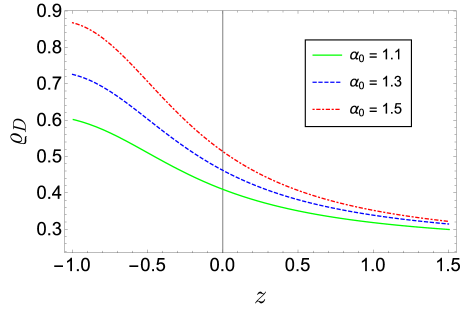
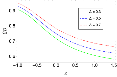
Figure 1: Evolution of $\rho_{D}$ versus $z$ for different values of $\alpha_{0}$ (upper panel) and $\Delta$ (lower panel) in non-interacting model. We have set $C=0.1$, $k=1.1$, $\alpha_{1}=0.9$, $\alpha_{2}=0.52$, $w=10$, $\phi_{0}=5$ and $\Delta=0.5$ in the upper panel, while $\alpha_{0}=1.1$ in the lower one (online colors).

In Fig. 2 we depict the evolution of the skewness parameter (15). We observe that it is negative and approaches constant values in the far future for selected values of $\alpha_{0}$ (upper panel) and $\Delta$ (lower panel). The same asymptotic behavior is exhibited in Raju for the case of a Kantowski-Sachs cosmological model with anisotropic dark energy fluid and massive scalar field.

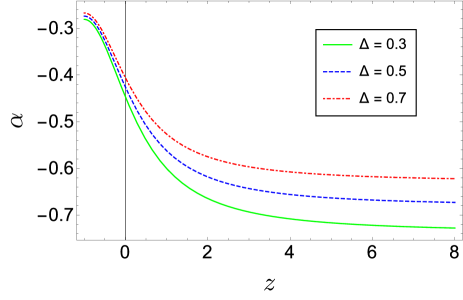
Figure 2: Evolution of skewness parameter versus $z$ for different values of $\alpha_{0}$ (upper panel) and $\Delta$ (lower panel) in non-interacting model. For all model parameters, we have set the same values as in Fig. 1 (online colors).

Now, from Eqs. (17), (21) and (24) we can derive the expression of the EoS parameter of BHDE as

$$\omega_{D} = -1\,-\frac{2\,e^{3\alpha_{0}t}\,\alpha_{0}^{5}\,\alpha_{1}^{\Delta-2}\left(\frac{\alpha_{0}}{\alpha_{1}+e^{-\alpha_{0}t}\,\alpha_{0}\alpha_{2}}\right)^{-\Delta}}{3C\left(k+2\right)^{2}\left(\alpha_{1}\,e^{\alpha_{0}t}+\alpha_{0}\alpha_{2}\right)^{5}}$$ (27)

$$\times\,\left\{\left(k-1\right)e^{\alpha_{0}t}\,\alpha_{0}\alpha_{1}-\left[\frac{\left(k+2\right)\left(\alpha_{1}\,e^{\alpha_{0}t}+\alpha_{0}\alpha_{2}\right)}{\alpha_{0}}\right]^{\frac{k}{2+k}}\right\}$$

$$+\,C\,e^{\alpha_{0}t}\,\alpha_{0}\,\alpha_{1}\,\alpha_{2}\left(\frac{\alpha_{0}\alpha_{1}}{\alpha_{1}+e^{-\alpha_{0}t}\alpha_{0}\alpha_{2}}\right)^{1-\Delta}\left(\Delta-2\right).$$

This is plotted in Fig. 3: from the upper panel we see that BHDE evolves from quintessence ($-1<\omega_{D}<-1/3$) at late time to approximately cosmological constant ($\omega_{D}=-1$) at present and phantom ($\omega_{D}<-1$) in the far future. In this regard, it is worth noting that largely negative values of $\omega_{D}$ indicate that the Universe might either end up with a big-rip or remain in the same current accelerating status.

By comparison with results of Santhi , we infer that the obtained behavior is peculiar to BHDE model in KS Universe. In fact, Tsallis HDE always lies in a quintessence-like regime and approaches cosmological constant in the far future. On the other hand, the same evolution is exhibited in the context of BHDE in Brans-Dicke Cosmology with a linear interaction Bar7 and Bianchi-type I BHDE in teleparallel gravity TeleBar . Furthermore, quantitative analysis gives us $\omega_{D_{0}}\in[-1.07,-0.99]$ for the current value of the EoS parameter and the considered values of $\alpha_{0}$. This is in good agreement with the recent constraint $\omega_{0}\in[-1.38,-0.89]$ obtained from Planck+WP+BAO measurements Planck . A qualitatively similar transition from quintessence to cosmological constant and phantom is displayed in the lower panel of Fig. 3 for fixed $\alpha_{0}$ and varying $\Delta$. In this case we find $\omega_{D_{0}}\in[-0.99,-0.95]$, which is still consistent with observations Planck .

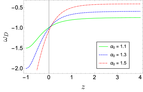
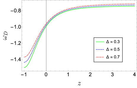
Figure 3: Evolution of EoS parameter versus $z$ for different values of $\alpha_{0}$ (upper panel) and $\Delta$ (lower panel) in non-interacting mode. For all model parameters, we have set the same values as in Fig. 1 (online colors).

Let us now investigate trajectories of $\omega_{D}-\omega_{D}^{\prime}$ plane. Here the overhead prime denotes derivative respect to the logarithm of the scale factor $a$, which is as usual related to the Hubble parameter by $H=\dot{a}/a$. $\omega_{D}-\omega_{D}^{\prime}$ plane has been introduced by Caldwell and Linder CL and represents a useful tool to distinguish among dark energy models. Firstly, it has been applied to quintessence model, which gives two different regions in this plane, i.e. the thawing ($\omega_{D}<0,\omega_{D}^{\prime}>0$) and freezing ($\omega_{D}<0,\omega_{D}^{\prime}<0$) domains. Subsequently, it has been generalized and extended to other dynamical dark energy models, see for instance Sche ; Chiba ; Guo ; Sharif . Cosmic trajectories of $\omega_{D}-\omega_{D}^{\prime}$ plane for the present framework are plotted in Fig. 4. We observe that our model predicts freezing region for BHDE, which is consistent with the current behavior of the Universe, since freezing regime is associated to a more accelerating era of cosmic expansion respect to thawing domain. The same result is exhibited in TeleBar for the case of BHDE in teleparallel gravity TeleBar , while the opposite scenario occurs in Tsallis HDE in KS Universe Santhi .

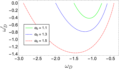
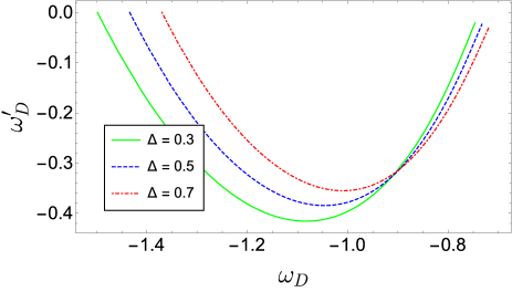
Figure 4: Evolution of $\omega_{D}-\omega^{\prime}_{D}$ trajectories for different values of $\alpha_{0}$ (upper panel) and $\Delta$ (lower panel) in non-interacting model. For all model parameters, we have set the same values as in Fig. 1 (online colors).

Another quantity that should be taken into account to establish whether a dark energy model is phenomenologically consistent is the deceleration parameter

$$q\,=\,-\frac{\ddot{a}}{aH^{2}}\,=\,-1-\frac{\dot{H}}{H^{2}}\,.$$ (28)

From this equation, we infer that positive values of $q$ correspond to a decelerated expansion of the Universe ($\ddot{a}<0$), while negative values characterize the accelerated regime ($\ddot{a}>0$). The behavior of $q$ is displayed in Fig. 5, showing that our model correctly reproduces the current accelerating phase of the cosmos. We emphasize that this is an advantage of BHDE scenario over standard HDE, which by contrast fails to explain the present accelerated expansion. Quantitatively speaking, for the selected values of $\alpha_{0}$ we find $q_{0}\in[-1.35,-1.23]$ for the current deceleration parameter. Although it slightly deviates from the standard $\Lambda$CDM model value $q_{0}=-0.55$ Planck , it overlaps with the estimation $q_{0}\in[-1.37,-0.79]$ recently obtained in Camerana via local supernovae measurements.

In Fig. 6 we present the evolution of the jerk parameter, which is a dimensionless third derivative of the scale factor respect to the cosmic time, i.e. Blandford:2004ah

$$j = \frac{1}{aH^{3}}\frac{d^{3}a}{dt^{3}}\,=\,q\left(2q+1\right)+\left(1+z\right)\frac{dq}{dz}$$ (29)

$$=\,1\,+\frac{9e^{-\frac{3\alpha_{0}}{1+(1+z)^{2}}}\alpha_{0}\alpha_{2}\left\{\left[2+z\left(2+z\right)\right]^{2}-2\left(1+z\right)^{2}\alpha_{0}\right\}}{\left[2+z\left(2+z\right)\right]^{2}\alpha_{1}}$$

$$+\,\frac{18e^{-\frac{6\alpha_{0}}{1+\left(1+z\right)^{2}}}\alpha_{0}^{2}\,\alpha_{2}^{2}}{\alpha_{1}^{2}}\,.$$

Figure 5: Evolution of deceleration parameter for different values of $\alpha_{0}$ in non-interacting model. For all model parameters, we have set the same values as in Fig. 1 (online colors).

We point out that the this parameter allows us to quantify deviations from $\Lambda$CDM model, which is indeed characterized by $j=1$. From Fig. 6 we can see that our model departs from $\Lambda$CDM at early times, while consistency is achieved in the far future. Also, we have $j_{0}\in[1.34,1.83]$ for the selected values of $\alpha_{0}$.

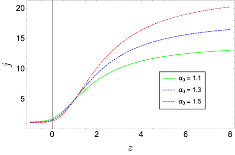
Figure 6: Evolution of jerk parameter for different values of $\alpha_{0}$ in non-interacting model. For all model parameters, we have set the same values as in Fig. 1 (online colors).

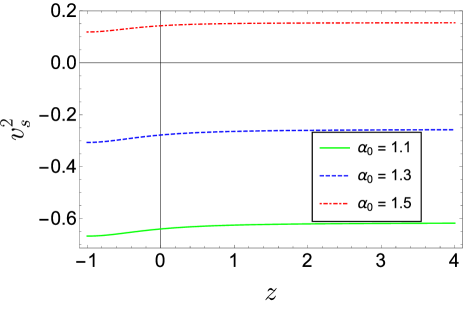
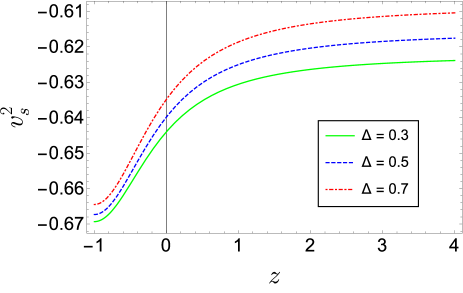
Figure 7: Evolution of squared speed of sound for different values of $\alpha_{0}$ (upper panel) and $\Delta$ (lower panel) in non-interacting model. For all model parameters, we have set the same values as in Fig. 1 (online colors).

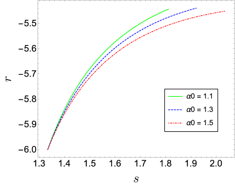
Figure 8: Evolution of $(r,s)$ plane trajectories for different values of $\alpha_{0}$. For all model parameters, we have set the same values as in Fig. 1 (online colors).

In order to study the classical stability of our model against small perturbations, let us now evaluate the squared speed of sound

$$v_{s}^{2}\,=\,\frac{\dot{p}_{D}}{\dot{\rho}_{D}}\,.$$ (30)

Notice that, in order for a given dark energy model to be stable, we must have $v_{s}^{2}>0$. Indeed, for a density perturbation, positive values of $v_{s}^{2}$ correspond to a regular propagation mode. On the other hand, for $v_{s}^{2}<0$ one has that the perturbation equation becomes an irregular wave equation, giving rise to an escalating mode Pert1 . In this setting, the pressure turns out to decrease when the density perturbation increases, thus favoring the development of an instability.

For the present BHDE model, we obtain the non-trivial expression

$$v_{s}^{2} = -1+C\alpha_{0}\,\alpha_{1}\,\alpha_{2}\left(\Delta-2\right)e^{\alpha_{0}t}H^{1-\Delta}\,+\,\frac{2\,\alpha_{1}^{2\Delta-5}}{3C}\bigg{\{}1-\alpha_{0}\alpha_{1}\left(k-1\right)e^{\alpha_{0}t}\left[\frac{\alpha_{1}(k+2)}{\alpha_{0}}\,e^{\alpha_{0}t}+\alpha_{2}\left(k+2\right)\right]^{-\frac{k}{2+k}}\bigg{\}}$$ (31)

$$\times\,\left[\frac{\alpha_{1}(k+2)}{\alpha_{0}}\,e^{\alpha_{0}t}+\alpha_{2}\left(k+2\right)\right]^{-\frac{4+k}{2+k}}\,H^{3-\Delta}\,+\,C\alpha_{0}\,\alpha_{1}\,\alpha_{2}\,\left(\Delta-2\right)e^{\alpha_{0}t}H^{-\left(1+\Delta\right)}\left[\left(1-\Delta\right)\dot{H}+\alpha_{0}\,H\right]\frac{H^{1-\Delta}}{(2-\Delta)\dot{H}}$$

$$+\,\frac{2\,\alpha_{1}^{2\Delta-5}H^{4-\Delta}}{3C\left(2-\Delta\right)\dot{H}}\left[\frac{\alpha_{1}(k+2)}{\alpha_{0}}\,e^{\alpha_{0}t}+\alpha_{2}\left(k+2\right)\right]^{-\frac{4+k}{2+k}}\Bigg{\{}\bigg{\{}1-\alpha_{0}\,\alpha_{1}\left(k-1\right)e^{\alpha_{0}t}\left[\frac{\alpha_{1}(k+2)}{\alpha_{0}}\,e^{\alpha_{0}t}+\alpha_{2}\left(k+2\right)\right]^{-\frac{k}{2+k}}\bigg{\}}$$

$$\times\,\bigg{\{}\left(3-\Delta\right)\frac{\dot{H}}{H}-\left(\frac{4+k}{2+k}\right)\left[\frac{\alpha_{1}(k+2)}{\alpha_{0}}\,e^{\alpha_{0}t}+\alpha_{2}\left(k+2\right)\right]^{-1}\bigg{\}}+\alpha_{0}^{2}\,\alpha_{1}\left(1-k\right)e^{\alpha_{0}t}\bigg{\{}\left[\frac{\alpha_{1}(k+2)}{\alpha_{0}}\,e^{\alpha_{0}t}+\alpha_{2}\left(k+2\right)\right]^{-\frac{k}{2+k}}$$

$$-\,\frac{\alpha_{1}\,k}{\alpha_{0}}\,e^{\alpha_{0}t}\left[\frac{\alpha_{1}(k+2)}{\alpha_{0}}\,e^{\alpha_{0}t}+\alpha_{2}\left(k+2\right)\right]^{-\frac{k+1}{2+k}}\bigg{\}}\Bigg{\}}\,.$$

This is plotted in Fig. 7 for different values of $\alpha_{0}$ (upper panel) and $\Delta$ (lower panel). From the upper panel, we see that the model is classically stable throughout the whole evolution for higher skewness (red curve), while it exhibits the opposite behavior as skewness decreases (green and blue curves), no matter the value of Barrow parameter (see lower panel). By contrast, SBT-based reconstruction of Tsallis HDE, as well as non-interacting BHDE in Brans-Dicke Cosmology are always unstable Santhi . This is a further advantage of our reconstruction.

Before moving onto the study of the interacting model, we focus on the statefinder diagnosis of BHDE. The statefinder parameters $r$ and $s$ were first introduced in rs to differentiate among the plethora of dark energy models. In the definition of these parameters, derivatives of the scale factor exceed the second order. In particular, we have

$$r \equiv \frac{\dddot{a}}{aH^{3}}\,,$$ (32)

$$s \equiv \frac{r-1}{3(q-\frac{1}{2})}\,.$$ (33)

We remind that the evolutionary trajectories of dark energy models in the $(r,s)$ plane can be classified as quintessence if $r<1$ and $s>0$ or Chaplygin gas if $r>1$ and $s<0$ class . For the present model we obtain Santhi

$$r = -\frac{\alpha_{0}^{2}\alpha_{2}\,e^{\alpha_{0}t}}{\alpha_{1}^{2}}\left[\frac{\alpha_{1}}{\alpha_{0}}+\alpha_{2}^{2}\left(1+2\,e^{-\alpha_{0}t}\right)\right]$$ (34)

$$+\,\frac{3\alpha_{0}\alpha_{2}\,e^{-\alpha_{0}t}}{\alpha_{1}}-6\,,$$

$$s = -\frac{2\alpha_{0}^{2}\alpha_{2}\,e^{-\alpha_{0}t}}{3\alpha_{1}\left(2\alpha_{0}\alpha_{2}\,e^{-\alpha_{0}t}-3\alpha_{1}\right)}\left[\frac{\alpha_{1}}{\alpha_{0}}+\alpha_{2}^{2}\left(1+2\,e^{-\alpha_{0}t}\right)\right]$$ (35)

$$+\frac{2\alpha_{0}\alpha_{1}\alpha_{2}\,e^{-\alpha_{0}t}\,-\,4\alpha_{1}}{\left(2\alpha_{0}\alpha_{2}\,e^{-\alpha_{0}t}-3\alpha_{1}\right)},$$

The trajectories of $(r,s)$ plane are plotted in Fig. 8, indicating that BHDE in this framework gives a correspondence with quintessence model.

III.2 Interacting model

Let us now examine how the above framework gets modified when considering a more realistic scenario with interacting dark matter and BHDE. In this case the continuity equation (13) can be split into the two relations

$$\dot{\rho}_{m}+3H\rho_{m}\,=\,Q\,,$$ (36)

$$\dot{\rho}_{D}+3H(1+\omega_{D})\rho_{D}+2\alpha\rho_{D}\frac{\dot{B}}{B}\,=\,-Q\,,$$ (37)

with $Q$ being the interaction term.

While there is no natural guidance from fundamental physics on the form of $Q$, phenomenological arguments have led to explore many possible scenarios over the years Q1 ; Q2 ; Q3 ; Q4 ; ComT0 ; ComT1 ; ComT2 . Following ComT0 ; ComT1 ; ComT2 , here we assume

$$Q=3\beta Hq\rho_{D}\,,$$ (38)

where $\beta$ is a dimensionless constant, which should take negative values according to observational measurements ComT1 .

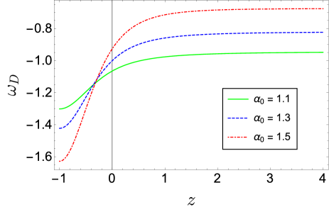
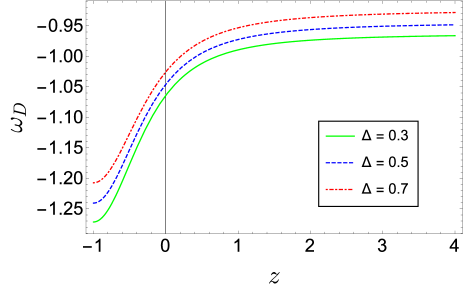
Figure 9: Evolution of EoS parameter for different values of $\alpha_{0}$ (upper panel), $\Delta$ (middle panel) and $\beta$ (lower panel) in interacting model. For all model parameters, we have set the same values as in Fig. 1. For the upper and middle panels, we have considered $\beta=-0.1$ (online colors).

Within this framework, the EoS parameter for dark energy becomes

$$\omega_{D} = -1\,-\frac{2\,e^{3\alpha_{0}t}\,\alpha_{0}^{5}\,\alpha_{1}^{\Delta-2}\left(\frac{\alpha_{0}}{\alpha_{1}+e^{-\alpha_{0}t}\,\alpha_{0}\alpha_{2}}\right)^{-\Delta}}{3C\left(k+2\right)^{2}\left(\alpha_{1}\,e^{\alpha_{0}t}+\alpha_{0}\alpha_{2}\right)^{5}}$$

$$\times\,\left\{\left(k-1\right)e^{\alpha_{0}t}\,\alpha_{0}\alpha_{1}-\left[\frac{\left(k+2\right)\left(\alpha_{1}\,e^{\alpha_{0}t}+\alpha_{0}\alpha_{2}\right)}{\alpha_{0}}\right]^{\frac{k}{2+k}}\right\}$$

$$+\,C\,e^{\alpha_{0}t}\,\alpha_{0}\,\alpha_{1}\,\alpha_{2}\left(\frac{\alpha_{0}\alpha_{1}}{\alpha_{1}+e^{-\alpha_{0}t}\alpha_{0}\alpha_{2}}\right)^{1-\Delta}\left(\Delta-2\right)\,-\,\beta q\,.$$

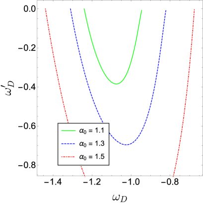
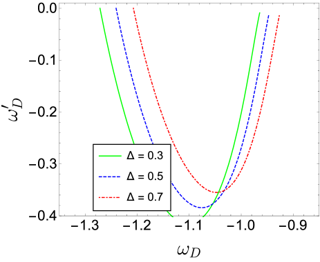
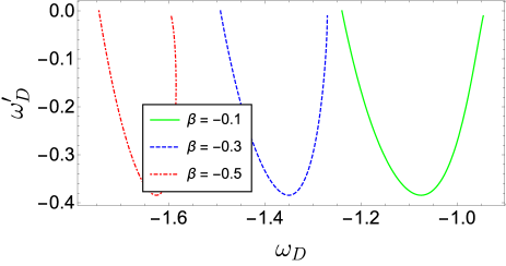
Figure 10: Evolution of $\omega_{D}-\omega^{\prime}_{D}$ trajectories for different values of $\alpha_{0}$ (upper panel), $\Delta$ (middle panel) and $\beta$ (lower panel) panel in interacting model. For all model parameters, we have set the same values as in Fig. 1. For the upper and middle panels, we have considered $\beta=-0.1$ (online colors).

For interaction small enough, the predicted evolution is qualitatively similar to the previous model, with the sequence of quintessence-, cosmological constant- and phantom-like behaviors (see upper and middle panels of Fig. 9). Estimation of the present value of $\omega_{D}$ now gives $\omega_{D_{0}}\in[-1.06,-0.92]$ for fixed $\Delta=0.5,\beta=-0.1$ and varying $\alpha_{0}$ (upper panel), and $\omega_{D_{0}}\in[-1.06,-1.02]$ for fixed $\alpha_{0}=1.1,\beta=-0.1$ and varying $\Delta$ (middle panel). Both these ranges are still in good agreement with observations (see the discussion below Eq. (27)). However, by increasing the magnitude of $\beta$, we find that BHDE always lies in the phantom regime (see blue and red curves in the lower panel), yielding $\omega_{D_{0}}\in[-1.61,-1.04]$. Therefore, we infer that large values of $\beta$ are phenomenologically disfavored, in line with the result of ComT1 .

Figure 10 displays the trajectories of $\omega_{D}-\omega^{\prime}_{D}$ phase plane. As for non-interacting model, they show that BHDE in SBT lies in the freezing domain.

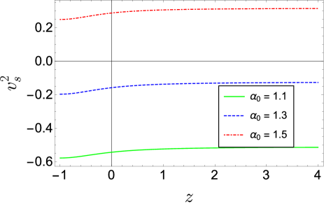
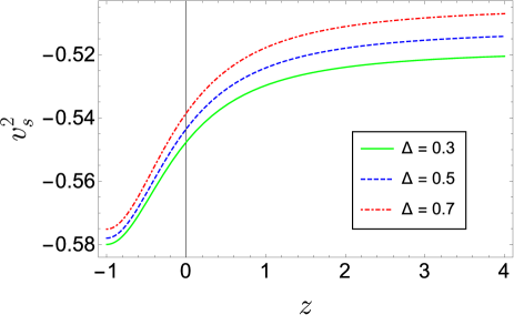
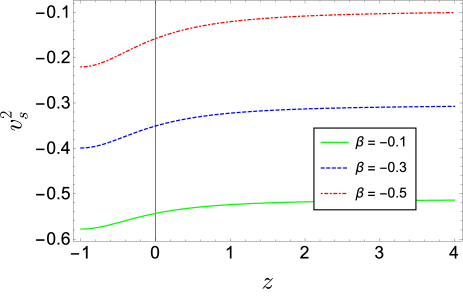
Figure 11: Evolution of squared speed of sound for different values of $\alpha_{0}$ (upper panel), $\Delta$ (middle panel) and $\beta$ (lower panel) in interacting model. For all model parameters, we have set the same values as in Fig. 1. For the upper and middle panels, we have considered $\beta=-0.1$ (online colors).

Let us finally consider how the classical stability is affected by Eq. (38). After some algebra, we find the following expression for the squared sound speed

$$v_{s}^{2} = -1+C\alpha_{0}\,\alpha_{1}\,\alpha_{2}\left(\Delta-2\right)e^{\alpha_{0}t}H^{1-\Delta}\,+\,\frac{2\,\alpha_{1}^{2\Delta-5}}{3C}\bigg{\{}1-\alpha_{0}\alpha_{1}\left(k-1\right)e^{\alpha_{0}t}\left[\frac{\alpha_{1}(k+2)}{\alpha_{0}}\,e^{\alpha_{0}t}+\alpha_{2}\left(k+2\right)\right]^{-\frac{k}{2+k}}\bigg{\}}$$ (40)

$$\times\,\left[\frac{\alpha_{1}(k+2)}{\alpha_{0}}\,e^{\alpha_{0}t}+\alpha_{2}\left(k+2\right)\right]^{-\frac{4+k}{2+k}}\,H^{3-\Delta}\,+\,C\alpha_{0}\,\alpha_{1}\,\alpha_{2}\,\left(\Delta-2\right)e^{\alpha_{0}t}H^{-\left(1+\Delta\right)}\left[\left(1-\Delta\right)\dot{H}+\alpha_{0}\,H\right]\frac{H^{1-\Delta}}{(2-\Delta)\dot{H}}$$

$$+\,\frac{2\,\alpha_{1}^{2\Delta-5}H^{4-\Delta}}{3C\left(2-\Delta\right)\dot{H}}\left[\frac{\alpha_{1}(k+2)}{\alpha_{0}}\,e^{\alpha_{0}t}+\alpha_{2}\left(k+2\right)\right]^{-\frac{4+k}{2+k}}\Bigg{\{}\bigg{\{}1-\alpha_{0}\,\alpha_{1}\left(k-1\right)e^{\alpha_{0}t}\left[\frac{\alpha_{1}(k+2)}{\alpha_{0}}\,e^{\alpha_{0}t}+\alpha_{2}\left(k+2\right)\right]^{-\frac{k}{2+k}}\bigg{\}}$$

$$\times\,\bigg{\{}\left(3-\Delta\right)\frac{\dot{H}}{H}-\left(\frac{4+k}{2+k}\right)\left[\frac{\alpha_{1}(k+2)}{\alpha_{0}}\,e^{\alpha_{0}t}+\alpha_{2}\left(k+2\right)\right]^{-1}\bigg{\}}+\alpha_{0}^{2}\,\alpha_{1}\left(1-k\right)e^{\alpha_{0}t}\bigg{\{}\left[\frac{\alpha_{1}(k+2)}{\alpha_{0}}\,e^{\alpha_{0}t}+\alpha_{2}\left(k+2\right)\right]^{-\frac{k}{2+k}}$$

$$-\,\frac{\alpha_{1}\,k}{\alpha_{0}}\,e^{\alpha_{0}t}\left[\frac{\alpha_{1}(k+2)}{\alpha_{0}}\,e^{\alpha_{0}t}+\alpha_{2}\left(k+2\right)\right]^{-\frac{k+1}{2+k}}\bigg{\}}\Bigg{\}}\,-\,\frac{\beta\dot{q}}{H}\,.$$

The behavior of $v_{s}^{2}$ is plotted in Fig. 11, indicating that increasing interactions might work in favor of a classical stabilization of the model against small perturbations (see the lower panel of Fig. 11, where it is shown that the larger the magnitude of $\beta$, the less stable BHDE becomes). More discussion on the above results can be found in the last Section, along with further directions to explore.

IV Observational constraints

IV.1 Hubble’s parameter

In order to explore the experimental consistency of reconstructed BHDE and constrain Barrow exponent $\Delta$, let us study the evolution of Hubble’s parameter $H(z)$ from Eq. (28). We develop our analysis for the non-interacting model and fixed parameters as in Sec. III, but similar considerations can be extended to the case when Eq. (38) is taken into account. Following TeleBar , we use data points obtained from 57 Hubble’s parameter measurements in the range $0.07\leq z\leq 2.36$. These points have been obtained through Differential Age (31 points), BAO and other methods (the remaining 26 points) and are outlined in Tab. 1 (see also TeleBar for more details).

$z$	$H(z)\,$	$\sigma_{H}$	$z\,$	$H(z)$	$\sigma_{H}$
0.070	69.0	19.6	0.4783	80	99
0.90	69	12	0.480	97	62
0.120	68.6	26.2	0.593	104	13
0.170	83	8	0.6797	92	8
0.1791	75	4	0.7812	105	12
0.1993	75	5	0.8754	125	17
0.200	72.9	29.6	0.880	90	40
0.270	77	14	0.900	117	23
0.280	88.8	36.6	1.037	154	20
0.3519	83	14	1.300	168	17
0.3802	83.0	13.5	1.363	160.0	33.6
0.400	95	17	1.430	177	18
0.4004	77.0	10.2	1.530	140	14
0.4247	87.1	11.2	1.750	202	40
0.4497	92.8	12.9	1.965	186.5	50.4
0.470	89	34

$z$	$H(z)\,$	$\sigma_{H}$	$z\,$	$H(z)$	$\sigma_{H}$
0.24	79.69	2.99	0.52	94.35	2.64
0.30	81.70	6.22	0.56	93.34	2.30
0.31	78.18	4.74	0.57	87.6	7.8
0.34	83.80	3.66	0.57	96.8	3.4
0.35	82.7	9.1	0.59	98.48	3.18
0.36	79.94	3.38	0.60	87.9	6.1
0.38	81.5	1.9	0.61	97.3	2.1
0.40	82.04	2.03	0.64	98.82	2.98
0.43	86.45	3.97	0.73	97.3	7.0
0.44	82.6	7.8	2.30	224.0	8.6
0.44	84.81	1.83	2.33	224	8
0.48	87.90	2.03	2.34	222.0	8.5
0.51	90.4	1.9	2.36	226.0	9.3

Table 1: 57 experimental points of $H(z)$ ($H$ is expressed in $\mathrm{km\,s^{-1}\,Mpc^{-1}}$ and $\sigma_{H}$ represents the uncertainty for each data point).

The best fit is found by employing the statistical $R^{2}$-test, which is defined by

$$R^{2}\,=\,1-\frac{\sum_{i=1}^{57}\left[(H_{i})_{ob}-(H_{i})_{th}\right]^{2}}{\sum_{i=1}^{57}\left[(H_{i})_{ob}-(H_{i})_{mean}\right]^{2}}\,,$$ (41)

where $(H_{i})_{ob}$ and $(H_{i})_{th}$ are the observed and predicted values of Hubble’s parameter, respectively. Minimizing the departure of $|R^{2}-1|$ from zero gives the constraint $\Delta\simeq 0.07$ at $95\%$ confidence level. This estimate is in line with recent predictions in literature Anagnostopoulos:2020ctz , though being less stringent than that obtained via Big Bang Nucleosynthesis measurements Barrow:2020kug . The fit in Fig. 12 also allows us to infer $H_{0}=(65.02\pm 4.3)\,\mathrm{km\,s^{-1}\,Mpc^{-1}}$, which is close to the recent observation from Planck Collaboration $H_{0}=\left(67.27\pm 0.60\right)\mathrm{km\,s^{-1}\,Mpc^{-1}}$ Planck , but deviates from $H_{0}=\left(74.03\pm 1.42\right)\mathrm{km\,s^{-1}\,Mpc^{-1}}$ derived from 2019 SH0ES collaboration SH0ES .

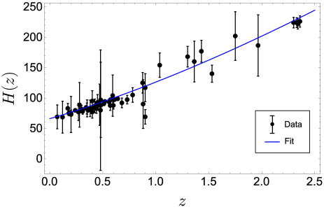
Figure 12: Best fit curve of Hubble’s parameter $H$ versus $z$. Dots represent data in Tab. 1, while the curve is the theoretical fit (online colors).

IV.2 Cosmological perturbations in BHDE

We now preliminarily investigate cosmological perturbations and structure formation in BHDE. For this analysis, we are inspired by Dago . In particular, we work in the linear regime on sub-horizon scales, studying the growth rate of matter fluctuations for clustering dark matter and a homogeneous dark energy component. More discussion along this line can be found in Sheykhi:2022gzb . For the case of weakly interacting dark components and scalar fluctuations of the metric in the Newtonian gauge, the line element (8) is modified by including a potential term $\phi$ as in Mukha . By introducing the density contrasts $\delta_{i}\equiv{\delta\rho_{i}}/{\rho_{i}}$ and divergences of the fluid velocities $\theta_{i}\equiv\vec{\nabla}\cdot\vec{v}_{i}$ for dark energy and dark matter, the evolution equations for the perturbations in the Fourier space take the form given in Abramo . We notice that DE effects on the growth of perturbations are only appreciable for $c^{2}_{eff}\equiv\delta p_{D}/\delta{\rho}_{D}\ll 1$, since in this case dark energy and dark matter cluster in a similar way (adiabaticity condition) Eric . On the other hand, $c^{2}_{eff}\simeq 1$ implies no growth because fluctuations would be suppressed by pressure. We can use evolution equations along with the relation $\frac{d}{dt}=\dot{a}\frac{d}{da}=aH\frac{d}{da}$ to extract differential equations for dark energy and matter perturbations in the form

$$\frac{d^{2}\delta_{m}}{da^{2}}+A_{m}\frac{d\delta_{m}}{da}+B_{m}\delta_{m} = S_{m}\,,$$ (42)

$$\frac{d^{2}\delta_{D}}{da^{2}}+A_{D}\frac{d\delta_{D}}{da}+B_{D}\delta_{D} = S_{D}\,,$$ (43)

where

$$A_{m} = \frac{3}{2a}\left(1-\omega_{D}\Omega_{D}\right)\,,$$ (44)

$$B_{m} = 0\,,$$ (45)

$$S_{m} = \frac{3}{2a^{2}}\left[\Omega_{m}\delta_{m}+\left(1+3c_{eff}^{2}\right)\Omega_{D}\delta_{D}\right],$$ (46)

$$A_{D} = \frac{1}{a}\left[\frac{3}{2}\left(1-\omega_{D}\Omega_{D}\right)-\frac{a}{1+\omega_{D}}\frac{d\omega_{D}}{da}-3\omega_{D}\right],$$ (47)

$$B_{D} = \frac{1}{a^{2}}\left[3\left(\frac{1}{2}-\frac{3}{2}\omega_{D}\Omega_{D}-\frac{a}{1+\omega_{D}}\frac{d\omega_{D}}{da}-3c^{2}_{eff}\right)\right.$$ (48)

$$\left.\times\,\left(c^{2}_{eff}-\omega_{D}\right)-3a\frac{d\omega_{D}}{da}+\frac{k}{a^{2}H^{2}}c^{2}_{eff}\right],$$

$$S_{D} = \frac{3}{2a^{2}}\left(1+\omega_{D}\right)\left[\Omega_{m}\delta_{m}+\left(1+3c_{eff}^{2}\right)\Omega_{D}\delta_{D}\right],$$ (49)

where $\Omega_{m}=\rho_{m}/\rho_{c}$ and $\Omega_{D}=\rho_{D}/\rho_{c}$ are the fractional energy density parameters of dark matter and BHDE, respectively, and $\rho_{c}=3m_{p}^{2}H^{2}$ the critical energy density. Hhere, $k$ identifies the (sub-horizon) scale in the Fourier space.

To solve the above equations, we need to impose initial conditions. Concerning $\delta_{m}$, perturbed Einstein equations lead to Dago

$$\delta^{(in)}_{m} = -2\phi_{(in)}\left(1+\frac{k^{2}}{3a^{2}_{(in)}H^{2}_{(in)}}\right),$$ (50)

$$\left(\frac{d\delta_{m}}{da}\right)^{(in)} = -\frac{2}{3}\frac{k^{2}\,\phi_{(in)}}{a^{2}_{(in)}H^{2}_{(in)}}\,.$$ (51)

Similarly, the adiabaticity condition gives for $\delta_{D}$ Kodama

$$\delta_{D}^{(in)} = \left(1+\omega_{D}\right)\delta_{m}^{(in)}\,,$$ (52)

$$\left(\frac{d\delta_{D}}{da}\right)^{(in)} = \left(1+\omega_{D}\right)\left(\frac{d\delta_{m}}{da}\right)^{(in)}+\frac{d\omega_{D}}{da}\delta_{m}^{(in)}\,.$$ (53)

For homogeneous BHDE (i.e. $\delta_{D}=0$), the following evolution for the linear matter perturbation on sub-horizon scales is obtained

$$\frac{d^{2}\delta_{m}}{da^{2}}+\left(\frac{3}{a}+\frac{1}{E}\frac{dE}{da}\right)\frac{d\delta_{m}}{da}-\frac{3\left(1-\Omega_{D}\right)}{2a^{2}}\delta_{m}\,=\,0\,,$$ (54)

where $E(a)$ is defined by

$$E(a)\equiv\frac{H(a)}{H_{0}}\,.$$ (55)

Now, from Eq. (54) we can calculate the growth rate of matter density perturbations as

$$f(a)\,\equiv\,a\,\frac{d\delta_{m}(a)}{da}\,.$$ (56)

We compare the above function with measurements of $f\sigma_{8}(a)\equiv f(a)\sigma_{8}(a)$ from redshift-space distortion observations for $0<z<1.5$ Boss , where $\sigma_{8}(a)=\sigma_{8}\delta_{m}(a)/\delta_{m}(1)$ is the linear-density field fluctuations in $8h^{-1}\,\mathrm{Mpc}$ radius and $\sigma_{8}$ its current value. We use the Gold-2017 dataset of 18 measurements of $f\sigma_{8}$ Nesseris , which are rescaled with respect to a given fiducial cosmological model. We consider $\Lambda$CDM as fiducial framework and introduce

$$r(z)\,=\,\frac{H(z)\hskip 0.56905ptd_{A}(z)}{H_{fid}(z)d_{A,fid}(z)}\,,$$ (57)

where

$$H_{fid}(z)\,=\,H_{0}\sqrt{\Omega_{m0}\left(1+z\right)^{3}+\left(1-\Omega_{m0}\right)}\,,$$ (58)

is the Hubble expansion rate in $\Lambda$CDM model. Measurements can then be corrected by means of the vector

$$\textbf{Y}\,=\,r(z_{i})\hskip 0.56905ptf\hskip 0.56905pt\sigma_{8}^{obs}(z_{i})-f\hskip 0.56905pt\sigma_{8}^{th}(z_{i})\,.$$ (59)

Thus, the likelihood function is given by $\mathcal{L}\,\propto\,e^{-\frac{1}{2}\hskip 0.56905pt\textbf{X}_{GRF}}$, where $\textbf{X}_{GRF}\,\equiv\,\textbf{Y}^{T}\,\textbf{C}_{GRF}^{-1}\,\textbf{Y}$ and $\textbf{C}_{GRF}$ is the covariance matrix of data listed in Tab. 2.

$z$	$f\sigma_{8}\,$	$z$	$f\sigma_{8}\,$
0.02	0.428 $\pm$ 0.0465	0.37	0.4602 $\pm$ 0.0378
0.02	0.398 $\pm$ 0.065	0.32	0.384 $\pm$ 0.095
0.02	0.314 $\pm$ 0.048	0.59	0.488 $\pm$ 0.060
0.10	0.370 $\pm$ 0.130	0.44	0.413 $\pm$ 0.080
0.15	0.490 $\pm$ 0.145	0.60	0.390 $\pm$ 0.063
0.17	0.510 $\pm$ 0.060	0.73	0.437 $\pm$ 0.072
0.18	0.360 $\pm$ 0.090	0.60	0.550 $\pm$ 0.120
0.38	0.440 $\pm$ 0.060	0.86	0.400 $\pm$ 0.110
0.25	0.3512 $\pm$ 0.0583	1.40	0.482 $\pm$ 0.116

Table 2: Dataset of 18 $f\sigma_{8}(z)$ measurements from different surveys Nesseris .

In Fig. 13 we show the growth rate of matter fluctuations for the BHDE (blue curve) model compared to the $\Lambda$CDM scenario (green curve). We see that the BHDE curve is nearly overlapped with the $\Lambda$CDM one at low redshifts. On the other hand, the two plots depart as $z$ increases, with the BHDE curve fitting high-redshift data better than $\Lambda$CDM. In particular, perturbations are found to grow up faster compared to predictions from the standard Cosmology. Such a discrepancy at high redshift can be understood by stressing that Barrow entropy is an effort to account for quantum-gravity corrections on the horizon surface. Clearly, these effects are expected to have more impact in the early Universe, when gravity should be quantum. A similar result has been recently exhibited in Sheykhi:2022gzb , where the faster growth of perturbations has been attributed to the exquisitely fractal structure of Universe horizon in Barrow framework, which can potentially work in favor of the growth of fluctuations of energy density.

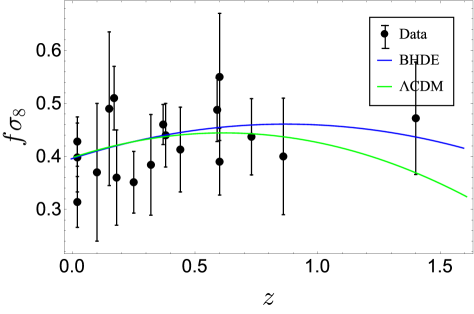
Figure 13: Growth of matter perturbations in BHDE (blue curve) and $\Lambda$CDM (green curve). We have set $\Delta=0.07$ and $\sigma_{8}=0.895$, $\delta^{(in)}_{m}=10^{-2}$, $(d\delta_{m}/da)^{(in)}=1$ as initial conditions Dago , while all other relevant parameters have been fixed as in Fig. 1 (online colors).

A final comment is in order here: to show the viability of a model, one needs complementary constraints by combing different observables. Indeed, single observational test cannot give solid sound result in principle. In this regard, we emphasize that cosmological models attempting to include quantum gravity effects in the standard Cosmology - like BHDE - are quite tough to test experimentally at present time, since quantum gravity effects (and their implications on the history of the Universe) are expected to be prominent in the very early Universe, where observational data are still lacking or not accurate enough. And in fact, constraints on Barrow entropy from relatively recent astrophysical/cosmological phenomena give very tiny deviations of Barrow parameter from zero, which in turn signal very small departure (if any) from Boltzmann-Gibbs entropy at that age (see, for instance, Bar6 ; Anagnostopoulos:2020ctz ; Barrow:2020kug ; LucianoInf ). In this sense, and also motivated by the analysis of Sheykhi:2022gzb , we have then realized that a useful test bench for Barrow proposal could be the study of growth rate factor data of matter fluctuations and structure formation, where even tiny gravitational effects might appear amplified as a result of the amplification of primordial density fluctuations. To further support the viability of this study, we remark that a similar constraint based on the growth of perturbations has been proposed in Dago for the case of Tsallis Holographic Dark Energy. Clearly, one can still insist on parallel tests of Barrow model with different observables. We stress that investigation along this direction is very active in recent literature Bar6 ; Anagnostopoulos:2020ctz ; Barrow:2020kug ; LucianoInf ; Lucianoarx ; Bar7 .

V Conclusions and Outlook

	Free parameters	Non-Interacting Model	Observational value
$\hskip 13.65732pt\omega_{D_{0}}$	(See Fig. 1)	$\hskip 41.25648pt[-1.07,-0.99]$	$[-1.38,-0.89]$ Planck
$q_{0}$	//	$\hskip 41.25648pt[-1.35,-1.23]$	$[-1.37,-0.79]$ Camerana
$j$	//	$j>0$ (for all $z$), $j(z\rightarrow-1)\rightarrow 1$	$j=1$ ($\Lambda$CDM)
$v_{s}^{2}$	//	$v_{s}^{2}<0$ (for $\alpha_{0}=1.1,1.3$) $v_{s}^{2}>0$ (for $\alpha_{0}=1.5$)	-
$\omega_{GT}-\omega^{\prime}_{GT}$	//	freezing	-
$H_{0}$	//	$(65.02\pm 4.3)\,\mathrm{km\,s^{-1}\,Mpc^{-1}}$	$\left(67.27\pm 0.60\right)\mathrm{km\,s^{-1}\,Mpc^{-1}}$ Planck

Table 3: Theoretical and observational values of EoS parameter, deceleration parameter, jerk parameter and squared sound speed for the best combination of arbitrary parameters of BHDE in SBT (for the jerk parameter we have considered the $\Lambda$CDM prediction as reference value).

In this work we have proposed a reconstruction of Barrow Holographic Dark Energy in Saez-Ballester theory of gravity. Motivated by recent observations from COBE, WMAP and Planck Ani0 ; Ani1 ; Ani , we have considered a Kantowski-Sachs Universe filled with dark matter and anisotropic BHDE as a background. To the best of our knowledge, this is the first time that BHDE is reconstructed in an anisotropic background like Kantowski-Sachs Universe. Indeed, all previous studies are framed in the standard homogeneous and isotropic FRW Universe. In this sense, all the results obtained in the present analysis are novel, as they account for anisotropic effects in the evolution of the Universe. By assuming the Hubble radius as an IR cutoff, we have investigated both the cases of non-interacting and interacting dark energy models, with special focus on the calculation of skewness parameter, Equation-of-State parameter, deceleration parameter, jerk parameter and squared sound speed. Among the main advantages over other descriptions of dark energy, we have shown that our model correctly reproduces the current accelerating phase of the cosmos, in contrast to standard HDE. Furthermore, the study of the squared speed of sound has revealed that our reconstruction is classically stable throughout the whole evolution of the Universe for higher skewness. By contrast, Saez Ballester-based reconstruction of Tsallis HDE, as well as non-interacting BHDE in Brans-Dicke Cosmology, are always unstable. Moreover, we have drawn the trajectories of $\omega_{D}-\omega^{\prime}_{D}$ phase plane and discussed statefinder diagnosis for non-interacting mdoel. In order to constrain free parameters, we have estimated current values of EoS parameter, jerk parameter and deceleration parameter, and compared them with recent measurements from Planck+WP+BAO. We have finally discussed the evolution of Hubble’s parameter and growth rate of matter fluctuations in BHDE. Results are summarized in Tab. 3, showing that SBT-based reconstruction of non-interacting BHDE is observationally consistent for $1.1<\alpha_{0}<1.5$, with large values of $\alpha_{0}$ being compatible with classical stability too. On the other hand, large (negative) interactions $\beta$ are phenomenologically disfavored, although they may contribute to stabilize the model against small perturbations.

Several aspects remain to be investigated:

• as discussed in Sec. III, our investigation correctly explains the behavior of various model parameters and the current accelerated expansion of the cosmos, though it does not predict its early-time decelerating phase. A possible explanation is that we are overlooking some ordinary matter DoF, which mostly contributed to the energy content in the early Universe and caused its initial deceleration. We reserve to improve our analysis in future investigation.

• In line with the study of LucianoPRD ; Mamon:2020spa ; Chakraborty:2021uzp , we aim at analyzing the thermodynamic implications of our model in order to establish whether it is thermally stable. This is essential to understand if SBT-based reconstruction of BHDE could clarify the yet unknown nature of DE. In this regard, we remark that thermal stability has been studied in LucianoPRD by considering the heat capacities and compressibilities of both interacting and non-interacting BHDE. It has been shown that such a model does not satisfy the Thermal Stability Condition. Moreover, in Lucianoarx the generalized second law (GSL) of thermodynamics has been analyzed by also including radiation effects in the energy budget of the Universe. Since the total entropy variation is not necessarily a non-negative function, a violation of the GSL can potentially occur. We emphasize that these results are in line with the achievement of Achiev for the case of Tsallis Holographic Dark Energy and, more general, with the outcome of Outc , where it has been found that DE fluids with a time-dependent EoS parameter are in conflict with the physical constraints imposed by thermodynamics. All the above results have been obtained for the usual FRW background. It would be interesting to explore whether and how they appear in the case of anisotropic spacetime, such as Kantowski-Sachs Universe considered here. This aspect is under active investigation and will be presented elsewhere.

• In Alleviate Abdalla et al. have argued that some HDE models can alleviate the $H_{0}$ tension since they predict $\omega_{D}<-1$, which seems a necessary condition to provide a solution based on late-time modifications LT . This requirement is met in both the two models considered above, potentially giving some glimpses toward the resolution of the $H_{0}$ tension. On other hand, in CapozLB it has been argued that the Hubble tension could be somehow removed if the look-back time is correctly referred to the redshift where the measurement is performed. This in turn rests upon the usage of the correct definition of $E(z)=H(z)/H_{0}$ in terms of the different contributions of radiation, matter, cosmological constant and spatial curvature to the density budget of the Universe. In this way, it has been shown that both values of the Hubble constant $H_{0}$ reported by the SH0ES and Planck collaborations Alleviate ; Khodadi can be recovered. It is suggestive to explore whether a similar dynamical resolution of the Hubble tension can be obtained in the context of BHDE. Although we are here working with a fixed IR cutoff, we envisage that some sort of correspondence between BHDE and look-back time approach can be still established by allowing Barrow parameter $\Delta$ to be varying on time. Preliminary studies along this direction have been presented recently in DiGennaro . More work along this direction is inevitably needed.

• BHDE is a generalization of standard Cosmology based on a deformation of the horizon entropy of the Universe. Extended cosmological scenarios, however, can also be obtained by modifying the geometric (i.e. gravitational) sector of Einstein-Hilbert action or motivated by thermodynamic requirements over the cosmological kinematics. In these directions, interesting approaches are provided by the Extended Gravity Cosmography EGC , which is a model-independent framework to tackle the dark energy/modified gravity problem, and the thermodynamic parametrization of dark energy TPDE . Hence, a possible outlook is to study BHDE in parallel with such generalized approaches and possibly reinterpret Barrow’s conjecture in this alternative language.

• In Sec. IV.2 we have discussed cosmological perturbations and structure formation neglecting anisotropy of spacetime. Clearly, a more comprehensive analysis requires including this feature too.

• A further challenging perspective is to extend the present analysis to the case of HDE based on Kaniadakis entropy Kana1 (Kaniadakis Holographic Dark Energy, KHDE), which is a self-consistent relativistic generalization of Boltzmann-Gibbs entropy parameterized by $-1<K<1$ GioKan ; LucRev , or HDE built on other commonly used entropies in physics, such as Abe, Landsberg-Vedral, Sharma-Mittal and Rény entropies. In this context, it would be interesting to find any connection between BHDE and such other models, and possibly constrain deformation parameters of these alternative modified entropies.

• A possible candidate for DE has been recently proposed in Capol1 ; Capol2 ; Capol3 by looking at the properties of the vacuum condensate of flavor mixed fields, in particular neutrinos Blas95 ; Luc23 . Although the origin of this alternative explanation is rooted in particle physics, it would be interesting to discuss these results in connection with our model of HDE. This may also allows us to extend the paradigm of Barrow entropy to the framework of particle physics.

• Finally, since our model attempts to include quantum gravitational effects into HDE, it is important to analyze our results in connection with predictions of more fundamental candidate theories of quantum gravity, such as String Theory, Loop Quantum Gravity and Asymptotically Safe Gravity, or phenomenological approaches, such as Planck-scale deformations of the Heisenberg principle KMM ; Scardigli ; LucGUP .

Work along these and other directions is still in progress and results will be presented elsewhere.

- (1) J. R. Primack, Nucl. Phys. B Proc. Suppl. 173, 1 (2007).
- (2) A. G. Riess et al. [Supernova Search Team], Astron. J. 116, 1009 (1998).
- (3) S. Perlmutter et al. [Supernova Cosmology Project], Astrophys. J. 517, 565 (1999).
- (4) D. N. Spergel et al. [WMAP], Astrophys. J. Suppl. 148, 175 (2003).
- (5) M. Tegmark et al. [SDSS], Phys. Rev. D 69, 103501 (2004).
- (6) P. A. R. Ade et al. [Planck], Astron. Astrophys. 571, A16 (2014).
- (7) S. Vagnozzi, L. Visinelli, P. Brax, A. C. Davis and J. Sakstein, Phys. Rev. D 104, 063023 (2021).
- (8) F. Ferlito, S. Vagnozzi, D. F. Mota and M. Baldi, Mon. Not. Roy. Astron. Soc. 512, 1885 (2022).
- (9) P. Salucci, G. Esposito, G. Lambiase, E. Battista, M. Benetti, D. Bini, L. Boco, G. Sharma, V. Bozza and L. Buoninfante, et al. Front. in Phys. 8, 603190 (2021).
- (10) S. Capozziello and M. De Laurentis, Phys. Rept. 509, 167 (2011).
- (11) A. G. Cohen, D. B. Kaplan and A. E. Nelson, Phys. Rev. Lett. 82, 4971 (1999).
- (12) P. Horava and D. Minic, Phys. Rev. Lett. 85, 1610 (2000).
- (13) S. D. Thomas, Phys. Rev. Lett. 89, 081301 (2002).
- (14) M. Li, Phys. Lett. B 603, 1 (2004).
- (15) S. D. H. Hsu, Phys. Lett. B 594, 13 (2004).
- (16) Q. G. Huang and M. Li, JCAP 08, 013 (2004).
- (17) S. Nojiri and S. D. Odintsov, Gen. Rel. Grav. 38, 1285 (2006).
- (18) B. Wang, C. Y. Lin and E. Abdalla, Phys. Lett. B 637, 357 (2006).
- (19) M. R. Setare, Phys. Lett. B 642, 421 (2006).
- (20) B. Guberina, R. Horvat and H. Nikolic, JCAP 01, 012 (2007).
- (21) L.N. Granda, A. Oliveros, Phys. Lett. B 671275, 199 (2009).
- (22) A. Sheykhi, Phys. Rev. D 84, 107302 (2011).
- (23) K. Bamba, S. Capozziello, S. Nojiri and S. D. Odintsov, Astrophys. Space Sci. 342, 155 (2012).
- (24) S. Ghaffari, M. H. Dehghani and A. Sheykhi, Phys. Rev. D 89, 123009 (2014).
- (25) S. Wang, Y. Wang and M. Li, Phys. Rept. 696, 1 (2017).
- (26) S. Nojiri and S. D. Odintsov, Eur. Phys. J. C 77 528 (2017).
- (27) H. Moradpour, A. H. Ziaie and M. Kord Zangeneh, Eur. Phys. J. C 80, 732 (2020).
- (28) X. Zhang and F. Q. Wu, Phys. Rev. D 72, 043524 (2005).
- (29) M. Li, X. D. Li, S. Wang and X. Zhang, JCAP 06, 036 (2009).
- (30) X. Zhang, Phys. Rev. D 79, 103509 (2009).
- (31) J. Lu, E. N. Saridakis, M. R. Setare and L. Xu, JCAP 03, 031 (2010).
- (32) S. Nojiri, S. D. Odintsov and E. N. Saridakis, Phys. Lett. B 797 134829 (2019).
- (33) S. Nojiri, S. D. Odintsov and V. Faraoni, Phys. Rev. D 105 044042 (2022).
- (34) S. Nojiri, S. D. Odintsov and T. Paul, Symmetry 13 928 (2021).
- (35) M. Tavayef, A. Sheykhi, K. Bamba and H. Moradpour, Phys. Lett. B 781, 195 (2018).
- (36) E. N. Saridakis, K. Bamba, R. Myrzakulov and F. K. Anagnostopoulos, JCAP 12, 012 (2018).
- (37) S. Nojiri, S. D. Odintsov and E. N. Saridakis, Eur. Phys. J. C 79, 242 (2019)..
- (38) G. G. Luciano and J. Gine, Phys. Lett. B 833, 137352 (2022).
- (39) N. Drepanou, A. Lymperis, E. N. Saridakis and K. Yesmakhanova, Eur. Phys. J. C 82, 449 (2022).
- (40) A. Hernández-Almada, G. Leon, J. Magaña, M. A. García-Aspeitia, V. Motta, E. N. Saridakis and K. Yesmakhanova, Mon. Not. Roy. Astron. Soc. 511, 4147 (2022).
- (41) G. G. Luciano, Eur. Phys. J. C 82, 314 (2022).
- (42) E. N. Saridakis, Phys. Rev. D 102, 123525 (2020).
- (43) M. P. Dabrowski and V. Salzano, Phys. Rev. D 102, 064047 (2020).
- (44) A. Sheykhi, Phys. Rev. D 103, 123503 (2021).
- (45) P. Adhikary, S. Das, S. Basilakos and E. N. Saridakis, Phys. Rev. D 104, 123519 (2021).
- (46) S. Nojiri, S. D. Odintsov and T. Paul, Phys. Lett. B 825, 136844 (2022).
- (47) G. G. Luciano and E. N. Saridakis, Eur. Phys. J. C 82, 558 (2022).
- (48) S. Ghaffari, G. G. Luciano and S. Capozziello, Eur. Phys. J. Plus 138, 82 (2023).
- (49) G. G. Luciano and J. Giné, [arXiv:2210.09755 [gr-qc]].
- (50) N. Boulkaboul, Phys. Dark Univ. 40, 101205 (2023).
- (51) P. S. Ens and A. F. Santos, EPL 131, 40007 (2020).
- (52) M. Zubair and L. R. Durrani, Chin. J. Phys. 69, 153 (2021).
- (53) M. Sharif and S. Saba, Symmetry 11, 92 (2019).
- (54) S. Waheed, Eur. Phys. J. Plus 135, 11 (2020).
- (55) S. Ghaffari, H. Moradpour, I. P. Lobo, J. P. Morais Graça and V. B. Bezerra, Eur. Phys. J. C 78, 706 (2018).
- (56) Y. Aditya, S. Mandal, P. K. Sahoo and D. R. K. Reddy, Eur. Phys. J. C 79, 1020 (2019).
- (57) Y. Liu, Eur. Phys. J. Plus 136, 579 (2021).
- (58) A. Sarkar and S. Chattopadhyay, Int. J. Geom. Meth. Mod. Phys. 18, 2150148 (2021).
- (59) G. G. Luciano, Phys. Rev. D 106, 083530 (2022).
- (60) M. Koussour, S. H. Shekh and M. Bennai, Int. J. Mod. Phys. A 37, 2250184 (2022).
- (61) J. D. Barrow, Phys. Lett. B 808, 135643 (2020).
- (62) D. Saez and V.J. Ballester, Phys. Lett. A 113, 467 (1986).
- (63) A. Pradhan, A. Kumar Singh and D. S. Chouhan, Int. J. Theor. Phys. 52, 266 (2013).
- (64) S. M. M. Rasouli and P. Vargas Moniz, Class. Quant. Grav. 35, 025004 (2018).
- (65) U. K. Sharma, R. Zia, A. Pradhan, J. Astrophys. Astr. 40, 2 (2019).
- (66) S. M. M. Rasouli, R. Pacheco, M. Sakellariadou and P. V. Moniz, Phys. Dark Univ. 27, 100446 (2020).
- (67) Y. Sobhanbabu and M. Vijaya Santhi, Eur. Phys. J. C 81, 1040 (2021).
- (68) H. Kim, Mon. Not. R. Astron. Soc. 364, 813 (2005).
- (69) A. H. Guth, Phys. Rev. D 23, 347 (1981).
- (70) A. Linde, Phys. Lett. B 108, 389 (1982).
- (71) R. Kantowski and R. K Sachs, J. Math. Phys 7, 3 (1966).
- (72) A. Sharma, K. Banerjee and J. Bhattacharyya, Phys. Rev. D 106, 063518 (2022).
- (73) W. J. Percival et al. [2dFGRS], Mon. Not. Roy. Astron. Soc. 327, 1297 (2001).
- (74) A. C. Pope et al. [SDSS], Astrophys. J. 607, 655 (2004).
- (75) K. Migkas, G. Schellenberger, T. H. Reiprich, F. Pacaud, M. E. Ramos-Ceja and L. Lovisari, Astron. Astrophys. 636, A15 (2020).
- (76) B. C. Paul, B. C. Roy and A. Saha, Eur. Phys. J. C 82, 76 (2022).
- (77) C. B. Collins, E. N. Glass and D. A. Wilkinson, Gen. Rel. Grav. 12, 805 (1980).
- (78) K.S. Adhav, Int. J. Astron. Astrophys. 1, 204 (2011).
- (79) M.V. Santhi et al., Can. J. Phys. 95, 179 (2017).
- (80) B. Wang, E. Abdalla, F. Atrio-Barandela and D. Pavon, Rept. Prog. Phys. 79, 096901 (2016).
- (81) F. K. Anagnostopoulos, S. Basilakos and E. N. Saridakis, Eur. Phys. J. C 80, 826 (2020).
- (82) J. D. Barrow, S. Basilakos and E. N. Saridakis, Phys. Lett. B 815, 136134 (2021).
- (83) G. G. Luciano, [arXiv:2301.12509 [gr-qc]].
- (84) N. Aghanim et al. [Planck], Astron. Astrophys. 641, A6 (2020) [erratum: Astron. Astrophys. 652, C4 (2021)].
- (85) A. G. Riess, S. Casertano, W. Yuan, L. M. Macri and D. Scolnic, Astrophys. J. 876, 85 (2019).
- (86) R. D’Agostino, Phys. Rev. D 99, 103524 (2019).
- (87) A. Sheykhi and B. Farsi, Eur. Phys. J. C 82, 1111 (2022).
- (88) V. F. Mukhanov, H. A. Feldman, R. Brandenberger, Phys. Rep. 215, 206 (1992).
- (89) L. R. Abramo, R. C. Batista, L. Liberato and R. Rosenfeld, Phys. Rev. D 79, 023516 (2009).
- (90) J. K. Erickson, R. R. Caldwell, P. J. Steinhardt, C. Armendariz-Picon and V. F. Mukhanov, Phys. Rev. Lett. 88, 121301 (2002).
- (91) H. Kodama and M. Sasaki, Prog. Theor. Phys. Suppl. 78, 1 (1984).
- (92) S. Alam et al. [BOSS], Mon. Not. Roy. Astron. Soc. 470, 2617 (2017).
- (93) S. Nesseris, G. Pantazis, L. Perivolaropoulos, Phys. Rev. D 96, 023542 (2017).
- (94) K. D. Raju, M. P. V. V. Bhaskara Rao, Y. Aditya, T. Vinutha and D. R. K. Reddy, Can. J. Phys. 98, 993 (2020).
- (95) R. R. Caldwell and E. V. Linder, Phys. Rev. Lett. 95, 141301 (2005).
- (96) R. J. Scherrer, Phys. Rev. D 73, 043502 (2006).
- (97) T. Chiba, Phys. Rev. D 73, 063501 (2006) [erratum: Phys. Rev. D 80, 129901 (2009)].
- (98) Z. K. Guo, Y. S. Piao, X. Zhang and Y. Z. Zhang, Phys. Rev. D 74, 127304 (2006).
- (99) M. Sharif and A. Jawad, Eur. Phys. J. C 72, 2097 (2012).
- (100) D. Camarena and V. Marra, Phys. Rev. Res. 2, 013028 (2020).
- (101) R. D. Blandford, M. A. Amin, E. A. Baltz, K. Mandel and P. J. Marshall, ASP Conf. Ser. 339, 27 (2005).
- (102) H. Kim, Mon. Not. Roy. Astron. Soc. 364, 813 (2005).
- (103) V. Sahni, T. D. Saini, A. A. Starobinsky and U. Alam, JETP Lett. 77, 201 (2003).
- (104) U. Alam, V. Sahni, T. D. Saini, A. A. Starobinsky, Mon. Not. Roy. Astron. Soc. 344, 1057 (2003).
- (105) H. Wei, Nucl. Phys. B 845, 381 (2011).
- (106) H. Wei, Commun. Theor. Phys. 56, 972 (2011).
- (107) Y. D. Xu and Z. G. Huang, Astrophys. Space Sci. 350, 855 (2014).
- (108) L. P. Chimento, A. S. Jakubi, D. Pavon and W. Zimdahl, Phys. Rev. D 67, 083513 (2003).
- (109) D. Pavon and W. Zimdahl, Phys. Lett. B 628, 206 (2005).
- (110) C. G. Boehmer, G. Caldera-Cabral, R. Lazkoz and R. Maartens, Phys. Rev. D 78, 023505 (2008).
- (111) G. Caldera-Cabral, R. Maartens and L. A. Urena-Lopez, Phys. Rev. D 79, 063518 (2009).
- (112) A. A. Mamon, A. Paliathanasis and S. Saha, Eur. Phys. J. Plus 136, 134 (2021).
- (113) G. Chakraborty, S. Chattopadhyay, E. Güdekli and I. Radinschi, Symmetry 13, 562 (2021).
- (114) M. Abdollahi Zadeh, A. Sheykhi and H. Moradpour, Gen. Rel. Grav. 51, 12 (2019).
- (115) E. M. Barboza, R. C. Nunes, E. M. C. Abreu and J. A. Neto, Phys. Rev. D 92, 083526 (2015).
- (116) E. Abdalla, G. Franco Abellán, A. Aboubrahim, A. Agnello, O. Akarsu, Y. Akrami, G. Alestas, D. Aloni, L. Amendola and L. A. Anchordoqui, et al. JHEAp 34, 49 (2022).
- (117) S. Vagnozzi, Phys. Rev. D 102, 023518 (2020).
- (118) S. Capozziello, G. Sarracino and A. D. A. M. Spallicci, Phys. Dark Univ. 40, 101201 (2023).
- (119) M. Khodadi and M. Schreck, Phys. Dark Univ. 39, 101170 (2023).
- (120) S. Di Gennaro and Y. C. Ong, Universe 8, 541 (2022).
- (121) S. Capozziello, R. D’Agostino and O. Luongo, Int. J. Mod. Phys. D 28, 1930016 (2019).
- (122) S. Capozziello, R. D’Agostino and O. Luongo, Phys. Dark Univ. 36, 101045 (2022).
- (123) G. Kaniadakis, Phys. Rev. E 66, 056125 (2002).
- (124) G.G. Luciano, Entropy 24, 1712 (2022).
- (125) A. Capolupo and A. Quaranta, Phys. Lett. B 840, 137889 (2023).
- (126) A. Capolupo and A. Quaranta, Phys. Lett. B 839, 137776 (2023)
- (127) A. Capolupo, Adv. High Energy Phys. 2018, 9840351 (2018).
- (128) M. Blasone and G. Vitiello, Annals Phys. 244, 283 (1995).
- (129) G. G. Luciano, Eur. Phys. J. Plus 138,, 83 (2023).
- (130) A. Kempf, G. Mangano and R. B. Mann, Phys. Rev. D 52, 1108 (1995).
- (131) F. Scardigli, Phys. Lett. B 452, 39 (1999).
- (132) G. G. Luciano, Eur. Phys. J. C 81, 672 (2021).