Combinatorial Inference on the Optimal Assortment in Multinomial Logit Models

Abstract

Assortment optimization has received active explorations in the past few decades due to its practical importance. Despite the extensive literature dealing with optimization algorithms and latent score estimation, uncertainty quantification for the optimal assortment still needs to be explored and is of great practical significance. Instead of estimating and recovering the complete optimal offer set, decision-makers may only be interested in testing whether a given property holds true for the optimal assortment, such as whether they should include several products of interest in the optimal set, or how many categories of products the optimal set should include. This paper proposes a novel inferential framework for testing such properties. We consider the widely adopted multinomial logit (MNL) model, where we assume that each customer will purchase an item within the offered products with a probability proportional to the underlying preference score associated with the product. We reduce inferring a general optimal assortment property to quantifying the uncertainty associated with the sign change point detection of the marginal revenue gaps. We show the asymptotic normality of the marginal revenue gap estimator, and construct a maximum statistic via the gap estimators to detect the sign change point. By approximating the distribution of the maximum statistic with multiplier bootstrap techniques, we propose a valid testing procedure. We also conduct numerical experiments to assess the performance of our method.

Keyword: Assortment optimization, combinatorial inference, multinomial logit model, multiplier bootstrap, hypothesis testing.

1 Introduction

Assortment optimization has generated extensive research interest due to its important implications in revenue management. Essentially, assortment optimization aims to study the balance between customer demand and product revenues, where the total expected revenues depend on the profits of individual products as well as customers’ preference rankings over the available products. Researchers propose various merchandising strategies to align the offered assortment with the customer decision-making process to maximize the expected revenues. A multitude of applications can be found in the fields of economics (Cachon et al.,, 2005; Çömez Dolgan et al.,, 2022), marketing (Mantrala et al.,, 2009; Kök et al.,, 2015), and operations (Blanchet et al.,, 2016; Aouad et al.,, 2018).

To model the customer choice behavior for assortment planning, many parametric models have been proposed, among which the multinomial logit (MNL) model (McFadden,, 1973) is one of the most popular due to its efficient algorithmic solutions to optimization problems. For a complete assortment of $n$ products, the MNL model associates each product with a preference score, and a customer’s willingness to purchase each product is proportional to the underlying preference scores, while there is a non-zero probability that customers may not purchase any product. The goal of assortment optimization is to solve for the optimal assortment that maximizes the expected revenues from the offered products. In real-world scenarios, it often delivers practical benefits to assess certain properties of the optimal assortment with quantified confidence levels and build the decision-making process upon it, which will be the primary concentration of this paper.

Previous studies have made significant progress in multiple topics regarding the choice models, including the MNL model, among which the algorithm to find the optimal offered assortment is the main focus in the operations research community. The tractable optimization solutions under the MNL model enabled previous studies to propose efficient assortment optimization algorithms (Talluri and Van Ryzin,, 2004; Gallego et al.,, 2004). Li et al., (2018) considered the assortment optimization for the two-stage MNL model based on an empirical estimation method using aggregated data. Other works attempted to generalize the MNL model by proposing new models to accommodate a broader range of choice behaviors, such as the nested logit model (NL) (Williams,, 1977), the generalized attraction model (GAM) (Gallego et al.,, 2015), the marginal distribution model (MDM) (Natarajan et al.,, 2009), and the group marginal distribution model (G-MDM) (Ruan et al.,, 2022). However, assortment optimization under those more general choice models may suffer from intractability. For instance, Rusmevichientong et al., 2010b and Davis et al., (2014) demonstrated that the assortment optimization is NP-hard for a mixture of MNL model and the nested logit model, respectively. Aouad et al., (2018) also characterized the hardness of approximation for assortment optimization under a general choice model by reducing the optimization problem to a computational problem of detecting large independent sets in graphs.

Apart from the intractable optimization solutions, the aforementioned works treated assortment planning as a deterministic process without accounting for the uncertainty induced by random input. Rusmevichientong and Topaloglu, (2012) brought the robustness against perturbation into the scope of assortment optimization under the MNL model by considering the robust optimization approach (Bertsimas and Sim,, 2004; Ahipaşaoğlu et al.,, 2019; Chen and Sim,, 2021; Chen et al., 2022a, ; Perakis et al.,, 2022; Zhu et al.,, 2022), where they aimed to find the optimal offer set that maximizes the worst-case expected revenue over an uncertain set of possible preference scores. However, the robust optimization is tailored to the worst-case scenario and will fail to quantify the uncertainty for general cases. Blanchet et al., (2016) proposed an alternative perspective to the same issue and proposed a Markov-chain-based model as a proper approximation to random utility-based discrete choice models, for which they provided an efficient algorithm. Nevertheless, this approach only approximated the true models without fundamentally addressing the uncertainty quantification.

As mentioned in the preceding discussion, despite the investigations of optimization algorithms, inferential analysis on the optimal assortment remains underexplored, especially considering the great significance of uncertainty quantification in practice (Lam et al.,, 2013; Jaillet et al.,, 2016). Taking the beverage industry (Akhigbe and Worlu,, 2020), for example, beverage retailers may ponder on whether to offer a beverage product they see from an advertisement to obtain maximal revenues. Considering the uncertainty of real-world data, to quantify their confidence in making such decisions, the retailers will need information beyond the estimation of the optimal assortment. For instance, the diverse sales records might lead the retailers to be more confident in one product but less confident in another, and the optimal assortment estimation per se can not capture such a difference. Therefore, we need uncertainty quantification to provide the decision-makers with a complete picture. We provide in the following some illustrative decision-making scenarios that merchandisers might be confronted with in practice. The decision on whether to offer a given product of interest is a popular topic in marketing (Zufryden,, 1986). More specifically, denote by $[n]=\{1,\ldots,n\}$ the full assortment of products, and by $\mathcal{S}^{*}$ the optimal offered assortment, we summarize the single product inclusion problem in the following example.

$\bullet$ Example 1. For a product $i$ of interest, we aim to test whether $i$ is in the optimal assortment.

$$\mathrm{H}_{0}:\text{Product }i\text{ is not in the optimal assortment ${\mathcal{S}}^{*}$,}$$

$$\mathrm{H}_{1}:\text{Product }i\text{ is in the optimal assortment ${\mathcal{S}}^{*}$}.$$

Apart from inferring the inclusion of a single product, research interest also lies in the shelf space allocation to different product categories (Curhan,, 1973) for profit maximization. Returning to the beverage industry example, retailers may wonder about allocating what proportion to each beverage category is the most profitable, e.g., whether to make more than 50% of the offered products on shelf alcoholic and less than 50% non-alcoholic. We formulate this application into the below hypothesis testing example.

$\bullet$ Example 2. For a given category of products $A=\{i_{1},\ldots,i_{K}\}$ and a given ratio $q\%$, we test if we should provide more than $q\%$ of the offered products from the category $A$ to maximize the revenues.

$$\mathrm{H}_{0}:\text{More than $q\%$ of ${\mathcal{S}}^{*}$ are from the category $A$,}$$

$$\mathrm{H}_{1}:\text{No larger than $q\%$ of ${\mathcal{S}}^{*}$ are from the category $A$}.$$

When there are several competitive beverage brands, the retailers may also be interested in which brand to choose as their major supplier. Such supplier selection problem is also important in marketing (Yücel et al.,, 2009), which we summarize in the example below.

$\bullet$ Example 3. For a partition $\{A_{1},\ldots,A_{m}\}$ of the products, we test if set $A_{1}$ constitutes the largest proportion of the optimal assortment ${\mathcal{S}}^{*}$ in comparison with all other $A_{j}$’s.

$$\mathrm{H}_{0}:\text{$A_{1}$ contains the most products in ${\mathcal{S}}^{*}$ compared with any other $A_{j}$'s,}$$

$$\mathrm{H}_{1}:\text{At least one of the other $A_{j}$'s contains more products in ${\mathcal{S}}^{*}$ than $A_{1}$}.$$

Note that the above inferential questions on partial properties of the optimal set do not require knowledge of the entire optimal assortment, and recovering the optimal offer set to answer such questions is inefficient since controlling uncertainty for the entire optimal assortment (i.e., the exact choice of all the products) is more challenging than controlling the uncertainty of only its partial properties (i.e., proportions of a given product category), which also explains why uncertainty quantification beyond estimation is of great practical importance. In summary, the aforementioned hypotheses aim to test whether the optimal assortment satisfies some given properties of interest. More generally, let $\boldsymbol{{\mathcal{S}}}$ be the set of all offer sets, i.e., all non-empty subsets of $[n]$, and let $\boldsymbol{{\mathcal{S}}}_{0}\subseteq{\boldsymbol{\mathcal{S}}}$ be a subset of offer sets satisfying certain properties of interest. We are interested in the following hypothesis testing problem on ${\mathcal{S}}^{*}$ that

$$\mathrm{H}_{0}:{\mathcal{S}}^{*}\in{\boldsymbol{\mathcal{S}}}_{0}\text{\leavevmode\nobreak\ versus\leavevmode\nobreak\ }\mathrm{H}_{1}:{\mathcal{S}}^{*}\notin{\boldsymbol{\mathcal{S}}}_{0}.$$ (1.1)

Examples 1 to 3 are concrete examples of the general hypothesis testing problem (1.1). In Section 2.2, we will provide an equivalent representation of (1.1) that will ease the computational difficulties caused by the combinatorial nature of assortment optimization and enable efficient inference.

1.1 Major Contributions

To the best of our knowledge, our paper provides the first inferential framework for performing general tests on the optimal assortment. Under the MNL choice model, our proposed method is able to test a large set of interesting properties of the optimal assortment, and we provide the theoretical guarantee for the validity of the test. We summarize our major contributions below.

$\bullet$ As far as we know, we are the first to provide the estimator’s rate of convergence under the MNL model, while previous studies mainly presented the MNL model under a deterministic framework and did not characterize the estimation error for random data. Our convergence rate is consistent with previous results under other choice models. We also propose a debiasing procedure under the MNL model to address the bias caused by penalized likelihood estimation, which paves the way for the follow-up inferential procedures.

$\bullet$ By reducing the properties test on the optimal assortment to a sign change point detection problem (Burg and Williams,, 2020), we provide a general inferential framework applicable to testing any arbitrary property under the MNL model. Specifically, we develop an inferential procedure based on multiplier bootstrap to construct a confidence interval for the optimal offer set, and apply the confidence interval to perform hypothesis testing on the optimal assortment. We also discuss concrete examples under the general framework, and by adapting to the case-specific settings, we may simplify the inferential procedure while maintaining the test validity.

$\bullet$ We characterize the estimation rate under the MNL model and provide theoretical guarantees for the validity of the general inferential procedure. In comparison with the ranking problems actively studied in recent literature (Chen et al., 2019b, ; Gao et al.,, 2021; Liu et al., 2022b, ), where the latent preference score is the sole parameter of interest and comparing the magnitudes of the preference scores alone is sufficient for inferring general ranking properties, inference problems in assortment optimization involve new dynamics between the revenues and the customer preferences, with the subject of interest being the result of a discrete optimization procedure. Thus inference in assortment optimization is more complex in nature and requires novel theories for uncertainty quantification.

1.2 Literature Review

The research on choice model has a long history, as reviewed above. Regarding the optimization problem under the MNL model, apart from the classic static assortment optimization (Ryzin and Mahajan,, 1999; Mahajan and Van Ryzin,, 2001), many variants of the MNL model have been proposed to incorporate additional information and make the model more realistic in practical scenarios. Several tracks of works include dynamic assortment optimization with adaptation to unknown customer choice behavior (Caro and Gallien,, 2007; Rusmevichientong et al., 2010a, ; Saure and Zeevi,, 2013; Agrawal et al.,, 2017; Chen and Wang,, 2018; Wang et al.,, 2018; Agrawal et al.,, 2019; Chen et al., 2020b, ), personalized assortment optimization integrating customer features (Golrezaei et al.,, 2014; Cheung and Simchi-Levi,, 2017; Chen et al., 2020a, ; Chen et al., 2022c, ), robust assortment optimization allowing for model misspecification (Besbes and Zeevi,, 2015; Chen et al., 2019a, ), and assortment optimization that restricts customer views to a subset of the offered assortment (Wang and Sahin,, 2018; Gallego et al.,, 2020; Aouad and Segev,, 2021). Specifically, Agrawal et al., (2019) proposed an efficient online algorithm that achieves simultaneous exploration and exploitation without requiring prior knowledge of instant parameters under the capacitated MNL model, and they achieved a near-optimal regret bound. Chen et al., 2020b took into consideration the time-varying features of products and adopted a changing contextual MNL model that allows the utility to be linearly dependent on the underlying time-evolving features, upon which they designed a dynamic policy to simultaneously learn the unknown features while making adaptive decisions for the offered assortment. Cheung and Simchi-Levi, (2017) studied the personalized MNL model where they assign each product with a fixed unknown coefficient and each customer with a known time-varying feature vector. To allow for outlier customer behavior, Chen et al., 2019a adopted the $\varepsilon$-contamination model, which assumes that a small proportion of the observations might be contaminated by an arbitrary distribution of choice behavior.

To maximize the expected revenues, aside from optimizing the offered assortment, pricing optimization provides an alternative perspective and enjoys a wealth of literature (Li et al.,, 2020; Yan et al.,, 2022; Liu et al., 2022a, ). For example, Yan et al., (2022) constructed a data-driven framework for solving the multi-product pricing problem, where they considered a separable representative consumer model (SRCM) to establish mathematical relationships between pricing and product demands. Liu et al., 2022a generalized the work of Yan et al., (2022) and studied a perturbed utility model (PUM) for modeling customers’ choice over subsets of primary products and ancillary services, and they achieved an efficient solution to the pricing problem by approximating the PUM with an additive perturbed utility model (APUM).

Since optimization problems in choice models usually entail knowledge of the latent parameters, recent choice model studies proposed various estimation methods to quantify the error rate resulting from random data. In terms of preference score estimation, the Bradley-Terry-Luce (BTL) model (Chen et al., 2019b, ) is among the most popular and is a special case of the MNL model with the offer set cardinality restricted to two and the no-purchase option removed. Many works in previous literature focused on estimating the preference scores and recovering the ranking of products under the BTL model. For instance, Chen et al., 2019b showed the optimality of both the MLE and spectral method up to some constant factor for the exact recovery of the top-$k$ ranking. Their results were further complemented by Chen et al., 2022b , who further dug into the leading constant factor of the optimal sample complexity and showed that the spectral method is sub-optimal when taking into account the leading constant, whereas the MLE is still optimal. Besides, Chen et al., 2022b established the minimax partial recovery rate for top-$k$ ranking problem under the BTL model. There are also works generalizing the estimation results to other choice models. For example, Mishra et al., (2012) proposed a parsimonious discrete choice model that avoids the Independence of Irrelevant Alternatives (IIA) and Invariant Proportion of Substitution (IPS) properties of the BTL model, and they estimated the choice probabilities through semidefinite optimization.

Apart from parameter estimation, uncertainty quantification also constitutes an important part of the ranking problems under the BTL model and is receiving recent research attention. For example, Gao et al., (2021) characterized the asymptotic normality of the MLE and spectral estimator under the sparse BTL model, which facilitates inferential analysis of the underlying scores. Liu et al., 2022b applied a Lagrangian debiasing correction to the regularized MLE and performed a general inference on the ranking properties based on the resulting estimator. Compared with the rich literature on score estimation, works on inferential analysis are greatly outnumbered in choice model studies, especially for assortment optimization. In this paper, we aim to bridge the gap by proposing a general inferential procedure that quantifies the uncertainty in assortment optimization.

Paper Organization. The rest of the paper is organized as follows. In Section 2, we provide the preliminary setup for optimal assortment inference under the multinomial logit (MNL) choice model, and we introduce some inference-related concepts to facilitate follow-up discussions. In Section 3, we propose our general inferential procedure for testing combinatorial properties of the optimal assortment, which is based upon a debiased likelihood estimator. We also provide a theoretical guarantee for the convergence rate of the estimator and show the validity of the inferential procedure. In Section 4, we perform numerical experiments on simulated data to evaluate the performance of our method on different hypothesis testing examples, followed by brief discussions in Section 5.

Notations. We denote by $|\cdot|$ the cardinality of a set. For two positive sequences $x_{n}$ and $y_{n}$, we denote $x_{n}\lesssim y_{n}$ or $x_{n}=O(y_{n})$ if there exists a positive constant $C>0$ independent of $n$ such that $x_{n}\leq Cy_{n}$ for all $n$ sufficiently large. We say $x_{n}\asymp y_{n}$ if $x_{n}\lesssim y_{n}$ and $y_{n}\lesssim x_{n}$. If $\lim_{n\rightarrow\infty}x_{n}/y_{n}=0$, then we say $x_{n}=o(y_{n})$. For two integers $j>i\geq 1$, denote by $[i]$ the set $\{1,2,\ldots,i\}$, by $i:j$ the set $\{i,i+1,\ldots,j\}$, and by $:$ the full index set. For a vector $\mathbf{v}=(v_{1},\ldots,v_{d})^{\top}$, we use $\|\mathbf{v}\|_{q}:=\left(\sum_{i=1}^{d}|v_{i}|^{q}\right)^{1/q}$ to denote the vector $\ell_{q}$-norm for an integer $q\geq 1$, and $\|\mathbf{v}\|_{\infty}:=\lim_{q\rightarrow\infty}\|\mathbf{v}\|_{q}=\max_{i}|v_{i}|$ to denote the vector $\ell_{\infty}$-norm. For a matrix ${\mathbf{A}}=[A_{ij}]$, we use $\|{\mathbf{A}}\|_{2}$ to denote the matrix spectral norm, $\|{\mathbf{A}}\|_{\infty}:=\sup_{\|\mathbf{x}\|_{\infty}=1}\|{\mathbf{A}}\mathbf{x}\|_{\infty}=\max_{i}\sum_{j}|A_{ij}|$ to denote the matrix $\ell_{\infty}$-norm, and $\|{\mathbf{A}}\|_{2,\infty}:=\sup_{\|\mathbf{x}\|_{2}=1}\|{\mathbf{A}}\mathbf{x}\|_{\infty}=\max_{i}\|{\mathbf{A}}_{i}\|_{2}$ to denote the 2-to-$\infty$ norm. We denote by $\mathbf{1}_{d}$ an $d$-dimensional vector with all entries equal to 1, and we omit the subscript when the dimension is clear from the context. We let $\{\boldsymbol{e}_{i}\}_{i=1}^{d}$ be the canonical basis for $\mathbb{R}^{d}$, where the dimension $d$ might change from place to place. Throughout the paper, we use $c,C$ to represent generic constants, whose values might change in different contexts.

2 Problem Setup

We provide the problem setup by briefly reviewing the assortment optimization problem under the multinomial logit model, followed by inferential analyses on the optimal assortment. Finally, we define the property sets corresponding to the optimal offer set to facilitate our discussions.

2.1 Multinomial Logit Choice Model

We consider the multinomial logit (MNL) model, in which the marginal probability for choosing one product of the offered assortment is proportional to the underlying preference scores associated with each product. More specifically, index by $[n]=\{1,\ldots,n\}$ the $n$ products and by 0 the no-purchase alternative. Define $[n]_{+}=[n]\cup\{0\}$. With each item $i\in[n]_{+}$, we assign a preference score $u_{i}^{*}>0$ and denote by $\bm{u}^{*}=(u_{0}^{*},u_{1}^{*},\ldots,u_{n}^{*})^{\top}$ the preference score vector. We let $\boldsymbol{\theta}^{*}=(\theta_{0}^{*},\theta_{1}^{*},\ldots,\theta_{n}^{*})^{\top}$ be the log-transformation of $\bm{u}^{*}$, where $\theta_{i}^{*}=\log(u_{i}^{*})$ for $i\in[n]_{+}$. We set $\theta_{0}^{*}=0$ to ensure identifiability since the model is invariant up to the constant shifting of $\theta_{i}^{*}$’s. We let the condition number of the preference scores be

$$\kappa_{\boldsymbol{\theta}}=\frac{\max_{i\in[n]_{+}}u_{i}^{*}}{\min_{i\in[n]_{+}}u_{i}^{*}}=\frac{\max_{i\in[n]_{+}}e^{\theta_{i}^{*}}}{\min_{i\in[n]_{+}}e^{\theta_{i}^{*}}},$$

and we consider the scenario where $\kappa_{\boldsymbol{\theta}}=O(1)$. We denote by $\mathcal{S}\subseteq[n]$ the offered assortment, i.e., the available set of products, and define $\mathcal{S}_{+}=\mathcal{S}\cup\{0\}$. Under the MNL model, the probability of choosing item $j\in\mathcal{S}_{+}$ is

$$\mathbb{P}(j\,|\,\mathcal{S}_{+})=\frac{u_{j}^{*}}{1+\sum_{i\in\mathcal{S}}u_{i}^{*}}=\frac{\exp(\theta_{j}^{*})}{1+\sum_{i\in\mathcal{S}}\exp(\theta_{i}^{*})},\quad\text{where }\theta_{0}^{*}=0.$$ (2.1)

Each item $i\in[n]_{+}$ is associated with a corresponding revenue parameter $r_{i}$, where $r_{0}=0$ for the no-purchase alternative. Without loss of generality, assume that we label the products such that $r_{1}\geq r_{2}\geq\ldots\geq r_{n}$. We introduce the condition number for the revenues as

$$\kappa_{r}=r_{1}/r_{n}.$$

Intuitively, a larger condition number indicates a less uniform distribution of revenues. Given an offered assortment $\mathcal{S}\subseteq[n]$, the total expected revenue is defined as

$$r(\mathcal{S})=\sum_{i\in\mathcal{S}}\frac{u_{i}^{*}r_{i}}{1+\sum_{j\in\mathcal{S}}u_{j}^{*}}.$$ (2.2)

We are interested in finding an optimal assortment that maximizes the total expected revenue that

$$\mathcal{S}^{\prime}\in\operatorname{argmax}_{\mathcal{S}\subseteq[n]}r(\mathcal{S}).$$ (2.3)

Since there may not be a unique optimal assortment, we focus on the smallest optimal assortment, i.e., the optimal assortment with the smallest cardinality, which we denote by $\mathcal{S}^{*}$.

Under the MNL model, the following theorem shows that the smallest optimal assortment $\mathcal{S}^{*}$ can be efficiently recovered at a low computational cost.

Theorem 2.1.

[Talluri and Van Ryzin, (2004)] Under the MNL model, the smallest optimal assortment $\mathcal{S}^{*}$ is of the form $\mathcal{S}^{*}=\{1,2,\ldots,K^{*}\}$ for some $K^{*}\in[n]$. Moreover, the following algorithm outputs the smallest optimal assortment $\mathcal{S}^{*}$:

1. For $k\in[n]$, calculate $\Delta_{k}=\sum_{i=1}^{k}r_{i}u_{i}^{*}-(\sum_{i=0}^{k}u_{i}^{*})r_{k}$. If $\Delta_{k}<0$, then $k\in\mathcal{S}^{*}$, and move on to $k=k+1$.

2. If $\Delta_{k}\geq 0$ or $k>n$, stop and output $\mathcal{S}^{*}=[k-1]$.

Note that the recovery of ${\mathcal{S}}^{*}$ in Theorem 2.1 requires the knowledge of $u_{i}^{*}$’s, which are not known to merchandisers in practice. We will discuss in Section 3 how to obtain ${\mathcal{S}}^{*}$ when $u_{i}^{*}$’s are unknown. With the concrete form of $\mathcal{S}^{*}$ in place, we are now ready to introduce the inference problem on $\mathcal{S}^{*}$.

2.2 Inference on the Optimal Offer Set

Recall that we aim to conduct inference on the smallest optimal offer set $\mathcal{S}^{*}$. In particular, we aim to perform general hypothesis testings as in (1.1). By Theorem 2.1, we see that under the MNL model the optimal set $\mathcal{S}^{*}$ takes the form $[K^{*}]$, where $K^{*}\in[n]$ is an integer. In other words, to optimize the total expected revenue, we will choose the products with the highest revenues while taking into account the customers’ chances of buying the products. Since knowing $\mathcal{S}^{*}$ and knowing $K^{*}$ are equivalent, we can see that the hypothesis testing in (1.1) in essence translates into testing whether set $K^{*}$ satisfies certain properties, e.g., Example 3 in Section 1 tests whether all the first $K^{*}$ products belong to a certain set $A$. Then we can reformulate the testing problem in (1.1) as that, for a given set $\mathcal{K}_{0}\subseteq[n]$, we test whether $K^{*}$ belongs to $\mathcal{K}_{0}$,

$$\mathrm{H}_{0}:K^{*}\in\mathcal{K}_{0}\text{\leavevmode\nobreak\ versus\leavevmode\nobreak\ }\mathrm{H}_{1}:K^{*}\notin\mathcal{K}_{0}.$$ (2.4)

We call $\mathcal{K}_{0}$ the property set of $K^{*}$. We formally introduce below the applications provided in Section 1 along with other examples and define the corresponding property set $\mathcal{K}_{0}$ as concrete formulations of (2.4).

Example 1.

For a given product $i\in[n]$, we test if $i$ is in the optimal assortment $\mathcal{S}^{*}$, i.e.,

$$\mathrm{H}_{0}:i\not\in\mathcal{S}^{*}\text{\leavevmode\nobreak\ versus\leavevmode\nobreak\ }\mathrm{H}_{1}:i\in\mathcal{S}^{*}.$$

The corresponding property set is $\mathcal{K}_{0}=\{k\in[n]:k\leq i-1\}$.

Example 2.

For a given set $A\subseteq[n]$, we test if $A$ is a subset of the optimal assortment $\mathcal{S}^{*}$, i.e.,

$$\mathrm{H}_{0}:A\nsubseteq\mathcal{S}^{*}\text{\leavevmode\nobreak\ versus\leavevmode\nobreak\ }\mathrm{H}_{1}:A\subseteq\mathcal{S}^{*}.$$

The corresponding property set is $\mathcal{K}_{0}=\{k\in[n]:k\leq(\max_{i\in A}i)-1\}$.

Example 3.

For a given set $A\subseteq[n]$, we test if the optimal assortment $\mathcal{S}^{*}$ is a subset of $A$, i.e.,

$$\mathrm{H}_{0}:\mathcal{S}^{*}\subseteq A\text{\leavevmode\nobreak\ versus\leavevmode\nobreak\ }\mathrm{H}_{1}:\mathcal{S}^{*}\nsubseteq A.$$

The corresponding property set is $\mathcal{K}_{0}=\{k\in[n]:\forall i\leq k,i\in A\}$.

Example 4.

For a given set $A\subseteq[n]$ and a given ratio $q\%$, we test if the proportion of $\mathcal{S}^{*}$ contained in $A$ is larger than $q\%$, i.e.,

$$\mathrm{H}_{0}:\lvert A\cap\mathcal{S}^{*}\rvert/\lvert\mathcal{S}^{*}\rvert>q\%\text{\leavevmode\nobreak\ versus\leavevmode\nobreak\ }\mathrm{H}_{1}:\lvert A\cap\mathcal{S}^{*}\rvert/\lvert\mathcal{S}^{*}\rvert\leq q\%.$$

The corresponding property set is $\mathcal{K}_{0}=\{k\in[n]:|[k]\cap A|/k>q\%\}$.

Example 5.

For a partition $\{A_{1},\ldots,A_{m}\}$ of the products, i.e., $\bigcup_{j=1}^{m}A_{j}=[n]$ and $A_{j}\cap A_{k}=\varnothing$ for $j\neq k$, we test if the products in $A_{1}$ constitute the largest proportion of the optimal assortment $\mathcal{S}^{*}$ in comparison with all the other $A_{j}$’s, i.e.,

$$\mathrm{H}_{0}:\lvert\mathcal{S}^{*}\cap A_{1}\rvert=\max_{j}\lvert\mathcal{S}^{*}\cap A_{j}\rvert\text{\leavevmode\nobreak\ versus\leavevmode\nobreak\ }\mathrm{H}_{1}:\lvert\mathcal{S}^{*}\cap A_{1}\rvert<\max_{j}\lvert\mathcal{S}^{*}\cap A_{j}\rvert.$$

The corresponding property set is $\mathcal{K}_{0}=\{k\in[n]:|[k]\cap A_{1}|=\max_{j}|[k]\cap A_{j}|\}$.

Example 6.

For a partition $\{A_{1},\ldots,A_{m}\}$ of the products, i.e., $\bigcup_{j=1}^{m}A_{j}=[n]$ and $A_{j}\cap A_{k}=\varnothing$ for $j\neq k$, we test if no less than $n_{0}$ out of the $m$ subsets $A_{j}$’s contain products that constitute the optimal assortment $\mathcal{S}^{*}$, where $n_{0}$ is a given count, i.e.,

$$\mathrm{H}_{0}:\lvert\{j\in[m]:A_{j}\cap\mathcal{S}^{*}\neq\varnothing\}\rvert\geq n_{0},$$

$$\mathrm{H}_{1}:\lvert\{j\in[m]:A_{j}\cap\mathcal{S}^{*}\neq\varnothing\}\rvert<n_{0}.$$

The corresponding property set is $\mathcal{K}_{0}=\{k\in[n]:|\{j\in[m]{:}\min_{i\in A_{j}}i\leq k\}|\geq n_{0}\}$.

We can see that the hypothesis testing on $\mathcal{S}^{*}$ is in essence testing whether the $K^{*}$ satisfies the properties of interest. In practice, the parameter $\boldsymbol{\theta}^{*}$ is unknown, and we will approximate $\boldsymbol{\theta}^{*}$ by its estimator $\widehat{\boldsymbol{\theta}}$ obtained from the observed data and estimate $\bm{u}^{*}$ by the plug-in $\widehat{\bm{u}}=\exp(\widehat{\boldsymbol{\theta}})$. Then we can estimate $\mathcal{S}^{*}$ by replacing $\Delta_{k}$ with $\widehat{\Delta}_{k}=\sum_{i=1}^{k}r_{i}\widehat{u}_{i}-(\sum_{i=0}^{k}\widehat{u}_{i})r_{k}$ in the algorithm proposed in Theorem 2.1. Besides, we can see from Theorem 2.1 that $k\in[n]$ belongs to $\mathcal{S}^{*}$ if and only if $\Delta_{k}<0$, and thus we can construct a confidence interval $[\widehat{K}_{L},\widehat{K}_{U}]$ of confidence level $1-\alpha$ for $K^{*}$ using $\{\widehat{\Delta}_{k}\}_{k\in[n]}$. Then we will reject ${\rm H}_{0}$ if $[\widehat{K}_{L},\widehat{K}_{U}]\cap\mathcal{K}_{0}=\varnothing$. We will discuss the method in more detail in the following section.

3 Method

In this section, we propose the algorithm for conducting general inferences on the optimal assortment ${\mathcal{S}}^{*}$. We begin by introducing how to estimate the latent preference scores from the observed data via a penalized optimization, and then provide a debiasing approach for the resulting estimator. Then we propose the inferential procedure based upon multiplier bootstrap to test arbitrary properties on the optimal offer set ${\mathcal{S}}^{*}$.

3.1 Observed Data and Latent Score Estimation

We first discuss the mechanism for collecting the observed data. In reality, the underlying preference scores $u_{i}^{*}$’s are unknown, and what merchandisers observe are the customers’ choice results among the offered assortments. Since there is an exponential number of possible assortments in total, in practice we may only observe the choice results for a subset of offer sets sampled from all the possible assortments. The goal is to estimate the latent preference scores from the observed data, and apply the estimators to the subsequent inference on ${\mathcal{S}}^{*}$.

More specifically, recall that ${\boldsymbol{\mathcal{S}}}$ is the set of all offer sets. We sample the observed offer sets from ${\boldsymbol{\mathcal{S}}}$ uniformly with probability $p$. More specifically, for each ${\mathcal{S}}\in{\boldsymbol{\mathcal{S}}}$, we define $\mathcal{E}_{{\mathcal{S}}}=1$ if the offer set ${\mathcal{S}}$ is selected and $\mathcal{E}_{{\mathcal{S}}}=0$ otherwise, and we assume that $\mathcal{E}_{{\mathcal{S}}}$ follows a Bernoulli distribution of probability $p$. We denote by $\boldsymbol{\mathcal{E}}=\{{\mathcal{S}}\in{\boldsymbol{\mathcal{S}}}:\mathcal{E}_{{\mathcal{S}}}=1\}$ the set of selected offer sets. For each selected offer set ${\mathcal{S}}$, we observe the choice results among the items in ${\mathcal{S}}_{+}$ for $L$ times independently. Here we assume the sample size $L$ to be the same for all selected sets for the simplicity of presentation. With some technical modifications, the theoretical analysis can be generalized to settings where the sample size $L_{{\mathcal{S}}}$ is different up to a constant factor for different sets ${\mathcal{S}}\in{\boldsymbol{\mathcal{S}}}$. We denote by $x_{{\mathcal{S}}}^{(i,\ell)}$ the choice outcome of the $\ell$-th customer for item $i$ in ${\mathcal{S}}_{+}$, and under the MNL model, $\{x_{{\mathcal{S}}}^{(i,\ell)}\}_{i\in{\mathcal{S}}_{+}}$ follow the following multinomial distribution

$$x_{{\mathcal{S}}}^{(i,\ell)}=\left\{\begin{array}[]{l}1,\text{ with probability }\frac{u_{i}^{*}}{1+\sum_{j\in{\mathcal{S}}}u_{j}^{*}}=\frac{e^{\theta_{i}^{*}}}{1+\sum_{j\in{\mathcal{S}}}e^{\theta_{j}^{*}}}\\ 0,\text{ otherwise }\end{array}\right.,\quad\theta_{0}^{*}=0,\quad\text{ for }{\mathcal{S}}\in{\boldsymbol{\mathcal{S}}}.$$ (3.1)

Then the negative log-likelihood function can be written as

$$\mathcal{L}(\boldsymbol{\theta};\bm{x})=-\sum_{{\mathcal{S}}\in\boldsymbol{\mathcal{E}}}\left\{\sum_{i\in{\mathcal{S}}}x_{{\mathcal{S}}}^{(i)}\theta_{i}-\log\left(1+\sum_{i\in{\mathcal{S}}}e^{\theta_{i}}\right)\right\},$$ (3.2)

where $x_{{\mathcal{S}}}^{(i)}=\frac{1}{L}\sum_{\ell=1}^{L}x_{{\mathcal{S}}}^{(i,\ell)}$. Let $\bm{x}=\{x_{{\mathcal{S}}}^{(i,\ell)}\}$ . We denote by $\widehat{\boldsymbol{\theta}}$ the penalized maximum likelihood estimate (MLE), which solves the following convex problem

$$\min_{\boldsymbol{\theta}\in\mathbb{R}^{n+1},\theta_{0}=0}\mathcal{L}_{\lambda}(\boldsymbol{\theta};\bm{x}):=\mathcal{L}(\boldsymbol{\theta};\bm{x})+\frac{\lambda}{2}\sum_{i\in[n]_{+}}(\theta_{i}-\bar{\theta})^{2},$$ (3.3)

where $\bar{\theta}=\sum_{i\in[n]_{+}}\theta_{i}/(n+1)$, and $\lambda>0$ is a tuning parameter. Here we regularize over the sample variance of $\theta_{i}$’s rather than the $\ell_{2}$-norm of $\boldsymbol{\theta}$ because the regularization over the sample variance of $\theta_{i}$’s will prevent $\theta_{i}$’s from getting too far away from their mean so as to exclude ill-conditioned $\boldsymbol{\theta}$. We characterize the convergence rate of $\widehat{\boldsymbol{\theta}}$ in the following theorem.

Theorem 3.1.

Recall that $\widehat{\boldsymbol{\theta}}$ is the regularized MLE. Under the conditions that $\lambda\asymp\sqrt{\frac{2^{n}p\log n}{nL}}$, $2^{n}p\geq Cn\log n$ for some large enough constant $C>0$ and $n\sqrt{\log n/(2^{n}pL)}\leq c$ for some small enough constant $c>0$ , with probability at least $1-O(n^{-10})$ we have that

$$\|\widehat{\boldsymbol{\theta}}-\boldsymbol{\theta}^{*}\|_{2}\lesssim n\sqrt{\frac{\log n}{2^{n}pL}}.$$ (3.4)

We refer interested readers to Supplementary Materials A for the proof of Theorem 3.1.

For each item $i\in[n]_{+}$, the observed number of purchases in each observation $\ell\in[L]$ is approximately $2^{n}p/n$ in expectation, i.e., $\mathbb{E}\big{(}\sum_{{\mathcal{S}}\in\boldsymbol{\mathcal{E}}:i\in{\mathcal{S}}}x_{{\mathcal{S}}}^{(i,\ell)}\big{)}\asymp 2^{n}p/n$, which is the amount of valid information for item $i$ for each observation. Theorem 3.1 indicates that we need to observe more than $\log n$ purchases of each item in each observation to obtain consistent estimation of $\boldsymbol{\theta}$. Besides, the total number of observed purchases across all $L$ observations for each item $i\in[n]$ needs to exceed $n\log n$, i.e., $2^{n}pL/n\gtrsim n\log n$. If one can sample more offer sets, the scaling condition on $L$ will be weaker.

3.2 Newton Debiasing with Centralization

Recall that $\widehat{\boldsymbol{\theta}}$ is the regularized MLE solving the problem (3.3), and we have the gradient and Hessian of $\mathcal{L}(\boldsymbol{\theta};\bm{x})$ as

$$\nabla\mathcal{L}(\boldsymbol{\theta};\bm{x})=-\sum_{{\mathcal{S}}\in\boldsymbol{\mathcal{E}}}\left\{\sum_{i\in{\mathcal{S}}_{+}}\left(x_{{\mathcal{S}}}^{(i)}-\frac{e^{\theta_{i}}}{\sum_{j\in{\mathcal{S}}_{+}}e^{\theta_{j}}}\right)\boldsymbol{e}_{i}\right\};$$ (3.5)

$$\nabla^{2}\mathcal{L}(\boldsymbol{\theta};\bm{x})=\sum_{{\mathcal{S}}\in\boldsymbol{\mathcal{E}}}\left\{\sum_{i\in{\mathcal{S}}_{+}}\frac{e^{\theta_{i}}(\sum_{j\in{\mathcal{S}}_{+},j\neq i}e^{\theta_{j}})}{\left(\sum_{j\in{\mathcal{S}}_{+}}e^{\theta_{j}}\right)^{2}}\boldsymbol{e}_{i}\boldsymbol{e}_{i}^{\top}-\sum_{\begin{subarray}{c}i,s\in{\mathcal{S}}_{+}\\ i\neq s\end{subarray}}\frac{e^{\theta_{i}}e^{\theta_{s}}}{\left(\sum_{j\in{\mathcal{S}}_{+}}e^{\theta_{j}}\right)^{2}}\boldsymbol{e}_{i}\boldsymbol{e}_{s}^{\top}\right\}.$$ (3.6)

Since the regularized estimation induces bias in the estimator, to perform inferential analysis based on $\widehat{\boldsymbol{\theta}}$, we need to correct for the bias first. We debias the regularized MLE $\widehat{\boldsymbol{\theta}}$ by a one-step Newton correction with centralization that

$$\widehat{\boldsymbol{\theta}}^{d}=\widehat{\boldsymbol{\theta}}^{\prime}-\nabla^{2}\mathcal{L}(\widehat{\boldsymbol{\theta}};\bm{x})^{\dagger}\nabla\mathcal{L}(\widehat{\boldsymbol{\theta}};\bm{x}),$$ (3.7)

where $\nabla^{2}\mathcal{L}(\widehat{\boldsymbol{\theta}};\bm{x})^{\dagger}$ is the Moore-Penrose inverse of the Hessian evaluated at $\widehat{\boldsymbol{\theta}}$ and $\widehat{\boldsymbol{\theta}}^{\prime}$ is the centralized MLE. Namely, $\widehat{\theta}_{i}^{\prime}=\widehat{\theta}_{i}-(n+1)^{-1}\sum_{j\in[n]_{+}}\widehat{\theta}_{j}$ for $i\in[n]_{+}$.

Here we apply centralization to $\widehat{\boldsymbol{\theta}}$ because by (3.6), we have $\nabla^{2}\mathcal{L}(\boldsymbol{\theta};\bm{x})^{\dagger}\mathbf{1}_{n+1}=\mathbf{0}$ for any $\boldsymbol{\theta}\in\mathbb{R}^{n+1}$, which indicates that due to the singularity of the Hessian matrix, the Newton correction will only correct bias on the direction perpendicular to $\mathbf{1}$. Hence to eliminate the bias on the direction of $\mathbf{1}$, we will first project $\widehat{\boldsymbol{\theta}}$ onto the perpendicular space of $\mathbf{1}$, i.e., apply centralization to $\widehat{\boldsymbol{\theta}}$. Besides, from (3.5) and (3.6) we can observe that $\nabla\mathcal{L}(\boldsymbol{\theta};\bm{x})$ and $\nabla^{2}\mathcal{L}(\boldsymbol{\theta};\bm{x})$ are invariant after adding a constant to $\boldsymbol{\theta}$, and hence the projection of $\widehat{\boldsymbol{\theta}}$ does not change the likelihood evaluation.

With the debiased estimator in place, we are now ready to present the inferential procedures. Recall from Section 2.2 that under the MNL model, the inference on the optimal offer set ${\mathcal{S}}^{*}$ is equivalent to the inference on its cardinality $K^{*}$. Furthermore, a product $k\in[n]$ is in ${\mathcal{S}}^{*}$ if and only if $\Delta_{k}<0$, where $\Delta_{k}$ is defined in Theorem 2.1. Thus, we see that $\Delta_{k}$’s serve as pivotal intermediate quantities in the inference of ${\mathcal{S}}^{*}$, and to provide uncertainty quantification for ${\mathcal{S}}^{*}$, we first provide uncertainty quantification for $\Delta_{k}$’s.

More specifically, for $k\in[n]$, we define $\widehat{\Delta}_{k}=\sum_{i=1}^{k}r_{i}\exp(\widehat{\theta}^{d}_{i})-\left(\sum_{i=0}^{k}\exp(\widehat{\theta}^{d}_{i})\right)r_{k}$, which is the estimator for $\Delta_{k}$ by plugging in the debiased estimator $\widehat{\boldsymbol{\theta}}^{d}$. Note that the centralization of $\widehat{\boldsymbol{\theta}}$ when calculating $\widehat{\boldsymbol{\theta}}^{d}$ will scale the plug-in estimators $\widehat{\Delta}_{k}$’s by a positive factor. However, since we are only interested in the signs of $\widehat{\Delta}_{k}$’s, the scaling of $\widehat{\Delta}_{k}$’s bears no impact on the inference. Hence with a slight abuse of notation, we redefine

$$\Delta_{k}=\sum_{i=1}^{k}r_{i}\exp(\theta^{*}_{i}-\bar{\theta}^{*})-\left(\!\sum_{i=0}^{k}\exp(\theta^{*}_{i}-\bar{\theta}^{*})\!\!\right)r_{k}=\exp(-\bar{\theta}^{*})\!\!\left(\sum_{i=1}^{k}r_{i}u_{i}^{*}-(\sum_{i=0}^{k}u_{i}^{*})r_{k}\right),\,\,k\in[n],$$

where $\bar{\theta}^{*}=(n+1)^{-1}\sum_{j\in[n]_{+}}\theta^{*}_{j}$. The following theorem depicts the asymptotic distribution of $\widehat{\Delta}_{k}$’s.

Theorem 3.2.

Under the same conditions as in Theorem 3.1, suppose that $\kappa_{r}=r_{1}/r_{n}\lesssim\sqrt{n}$ and ${n^{2}\log n}/{\sqrt{2^{n}pL}}=o(1)$. Then, for all $k\in[n]$, we have that

$$\sqrt{\frac{L}{\mathbf{v}_{k}^{\top}\nabla^{2}\mathcal{L}(\boldsymbol{\theta}^{*};\bm{x})^{\dagger}\mathbf{v}_{k}}}(\widehat{\Delta}_{k}-\Delta_{k})\overset{d}{\longrightarrow}N(0,1),$$ (3.8)

where $\mathbf{v}_{k}={\exp(-\bar{\theta}^{*})}\cdot\big{(}{(0-r_{k})u_{0}^{*},(r_{1}-r_{k})u_{1}^{*},(r_{2}-r_{k})u_{2}^{*},\ldots,(r_{k-1}-r_{k})u_{k-1}^{*}},0,\ldots,0\big{)}^{\top}$.

The proof of Theorem 3.2 is deferred to Supplementary Materials B. Compared with Theorem 3.1, we have an extra scaling condition on the condition number $\kappa_{r}$ to ensure that the revenue parameters are not ill-conditioned. Besides, we have a stronger scaling condition on the sample size $L$ to guarantee distributional convergence. Since $\boldsymbol{\theta}^{*}$ is unknown in practice, we estimate the asymptotic variance by plugging in the regularized MLE $\widehat{\boldsymbol{\theta}}$. The following corollary of Theorem 3.2 shows the validity of the plug-in estimate.

Corollary 3.3.

Under the same conditions as Theorem 3.2, we have

$$\sqrt{\frac{L}{\widehat{\mathbf{v}}_{k}^{\top}\nabla^{2}\mathcal{L}(\widehat{\boldsymbol{\theta}};\bm{x})^{\dagger}\widehat{\mathbf{v}}_{k}}}(\widehat{\Delta}_{k}-\Delta_{k})\overset{d}{\longrightarrow}N(0,1),$$ (3.9)

where $\widehat{\mathbf{v}}_{k}=\Big{(}{(0-r_{k})\widehat{u}_{0},(r_{1}-r_{k})\widehat{u}_{1},(r_{2}-r_{k})\widehat{u}_{2},\ldots,(r_{k-1}-r_{k})\widehat{u}_{k-1}},0,\ldots,0\Big{)}^{\top}$ with $\widehat{u}_{i}=\exp(\widehat{\theta}_{i}^{\prime})$.

See Supplementary Materials C for the proof of Corollary 3.3. Based upon the asymptotic normality of $\Delta_{k}$’s, we are ready to formally introduce the inferential procedure in the next section.

3.3 Hypothesis Testing for ${\mathcal{S}}^{*}$

In this section, we will perform a general inference on ${\mathcal{S}}^{*}$ to test whether it satisfies certain properties of interest. As established in Section 2.2, the general hypothesis testing for ${\mathcal{S}}^{*}$ defined in (1.1) is equivalent to the following test on $K^{*}$,

$$\mathrm{H}_{0}:K^{*}\in\mathcal{K}_{0}\text{\leavevmode\nobreak\ versus\leavevmode\nobreak\ }\mathrm{H}_{1}:K^{*}\notin\mathcal{K}_{0},$$

where $\mathcal{K}_{0}$ is the property set of $K^{*}$ satisfying certain properties. Then to perform the inference on $K^{*}$, for a given level $\alpha\in(0,1)$, we utilize the equivalence between the events $\{k\in{\mathcal{S}}^{*}\}$ and $\{\Delta_{k}<0\}$, and construct a confidence interval of confidence level $1-\alpha$ for $K^{*}$. Specifically, we define the maximal statistic

$$T=\max_{k\in[n]}\big{(}{\widehat{\Delta}_{k}-\Delta_{k}}\big{)}\Big{/}{\sqrt{\widehat{\mathbf{v}}_{k}^{\top}\nabla^{2}\mathcal{L}(\widehat{\boldsymbol{\theta}};\bm{x})^{\dagger}\widehat{\mathbf{v}}_{k}/L}},$$ (3.10)

and we construct the confidence interval of $K^{*}$ by estimating the quantile of $T$. We consider the Gaussian multiplier bootstrap proposed in Chernozhukov et al., (2013) for estimating the quantile of $T$, which approximates the maximum of a sum of random vectors by the empirical quantiles of Gaussian maximum. In particular, we define the following statistic as the approximation of $T$,

$$W=\max_{k\in[n]}\sum_{\ell=1}^{L}\left\{\frac{\widehat{\mathbf{v}}_{k}^{\top}\nabla^{2}\mathcal{L}(\widehat{\boldsymbol{\theta}};\bm{x})^{\dagger}}{\sqrt{L\cdot\widehat{\mathbf{v}}_{k}^{\top}\nabla^{2}\mathcal{L}(\widehat{\boldsymbol{\theta}};\bm{x})^{\dagger}\widehat{\mathbf{v}}_{k}}}\sum_{S\in\mathcal{I}}\mathcal{E}_{S}\left\{\sum_{i\in S}\left(x_{S}^{(i,\ell)}-\frac{e^{\widehat{\theta}_{i}}}{\sum_{j\in S}e^{\widehat{\theta}_{j}}}\right)\boldsymbol{e}_{i}\right\}z_{S,\ell}\right\},$$ (3.11)

where $\{z_{S,\ell}\}_{\ell=1}^{L}$ are i.i.d. standard Gaussian, and $\mathcal{E}_{S}=1$ if $S$ is selected for the observed data and $\mathcal{E}_{S}=0$ otherwise. For a given level $\alpha\in(0,1)$, we define the quantile of $W$ conditional on the data $\bm{x}$ and the selected sets $\mathcal{E}$ as

$$c_{W}(\alpha,\boldsymbol{\mathcal{E}})=\inf\{t\in\mathbb{R}:\mathbb{P}(W>t\,|\,\boldsymbol{x},\boldsymbol{\mathcal{E}})\leq\alpha\}.$$ (3.12)

We will show that $W$ approximates $T$, and $c_{W}(\alpha,\boldsymbol{\mathcal{E}})$ approximates $T$’s $\alpha$-quantile under some mild conditions. Then we can establish a $(1-\alpha)$-level confidence interval for $K^{*}$: $[\widehat{K}_{L},\widehat{K}_{U}]$, where

$$\widehat{K}_{L}=\max\Bigg{\{}k:\widehat{\Delta}_{k}<-c_{W}(\frac{\alpha}{2},\boldsymbol{\mathcal{E}})\sqrt{\frac{\widehat{\mathbf{v}}_{k}^{\top}\nabla^{2}\mathcal{L}(\widehat{\boldsymbol{\theta}};\bm{x})^{\dagger}\widehat{\mathbf{v}}_{k}}{L}}\Bigg{\}},$$

$$\widehat{K}_{U}=\max\Bigg{\{}k:\widehat{\Delta}_{k}\leq c_{W}(\frac{\alpha}{2},\boldsymbol{\mathcal{E}})\sqrt{\frac{\widehat{\mathbf{v}}_{k}^{\top}\nabla^{2}\mathcal{L}(\widehat{\boldsymbol{\theta}};\bm{x})^{\dagger}\widehat{\mathbf{v}}_{k}}{L}}\Bigg{\}}.$$

We summarize the framework of constructing the confidence interval in Algorithm 1.

Define the parameter space of $\boldsymbol{\theta}^{*}$ as $\mathbf{\Theta}=\{\theta:\kappa_{\theta}\leq C_{\kappa}\}$, where $C_{\kappa}$ is a constant independent of $n$. Then the following theorem shows the validity of the testing procedure based on the confidence interval for $K^{*}$.

Theorem 3.4.

Under the same conditions as Theorem 3.1, suppose $\kappa_{r}\lesssim\sqrt{n}$, and $n^{2}\sqrt{(\log n)^{3}/(2^{n}pL)}=o(1)$. Then, for any level $0<\alpha<1$, we have that

$$\liminf_{n,L\rightarrow\infty}\inf_{\boldsymbol{\theta}^{*}\in\mathbf{\Theta}}\mathbb{P}_{\boldsymbol{\theta}^{*}}(K^{*}\in[\widehat{K}_{L},\widehat{K}_{U}])\geq 1-\alpha.$$ (3.13)

Moreover,

$$\limsup_{n,L\rightarrow\infty}\sup_{\boldsymbol{\theta}^{*}:{\mathcal{S}}^{*}\in{\boldsymbol{\mathcal{S}}}_{0}}\mathbb{P}_{\boldsymbol{\theta}^{*}}(\text{\rm Reject }H_{0})\leq\alpha.$$ (3.14)

We give below a proof sketch of Theorem 3.4 to facilitate understanding. The detailed proof is provided in Section E.

Proof.

Proof Sketch. The proof contains three steps. First, we reduce quantifying the uncertainty of ${\mathcal{S}}^{*}$ to quantifying the uncertainty of the sign change point detection based on the maximal scaled estimation error $T$. Second, we show that the multiplier bootstrap quantile $c_{W}(\alpha,\boldsymbol{\mathcal{E}})$ is valid and in turn, the confidence interval is valid. Third, based on the equivalence between the two hypothesis tests (1.1) and (2.4), we establish the asymptotic validity of our inferential procedure.

Step 1. By previous arguments, we establish the equivalence of the following events:

$$\{k\in{\mathcal{S}}^{*}\}=\{k\leq K^{*}\}=\{\Delta_{k}<0\},$$

which indicates that making inference on ${\mathcal{S}}^{*}$ is equivalent to inferring the signs of $\Delta_{k}$’s. Moreover, we have the following lower bound for the coverage probability

$$\mathbb{P}(K^{*}\in[\widehat{K}_{L},\widehat{K}_{U}])\geq 1\!-\!\mathbb{P}(\widehat{K}_{L}\!>\!K^{*})\!-\!\mathbb{P}(\widehat{K}_{U}\!+\!1\!\leq\!K^{*})\geq 1\!-\!\mathbb{P}(\Delta_{\widehat{K}_{L}}\!\geq\!0)-\mathbb{P}\left(\Delta_{\widehat{K}_{U}+1}\!<\!0\right).$$

By our definition of $\widehat{K}_{L}$ and $\widehat{K}_{U}$, the estimators of $\Delta_{\widehat{K}_{L}}$ and $\Delta_{\widehat{K}_{U}+1}$ failing to predict the signs means that the estimation errors of both $\widehat{\Delta}_{\widehat{K}_{L}}$ and $\widehat{\Delta}_{\widehat{K}_{U}+1}$ exceed the cut-off threshold, i.e.,

$$\widehat{\Delta}_{\widehat{K}_{L}}-\Delta_{\widehat{K}_{L}}<-c_{W}(\frac{\alpha}{2},\boldsymbol{\mathcal{E}})\sqrt{\frac{\widehat{\mathbf{v}}_{\widehat{K}_{L}}^{\top}\nabla^{2}\mathcal{L}(\widehat{\boldsymbol{\theta}};\bm{x})^{\dagger}\widehat{\mathbf{v}}_{\widehat{K}_{L}}}{L}},$$

$$\widehat{\Delta}_{\widehat{K}_{U}+1}-\Delta_{\widehat{K}_{U}+1}>c_{W}(\frac{\alpha}{2},\boldsymbol{\mathcal{E}})\sqrt{\frac{\widehat{\mathbf{v}}_{\widehat{K}_{U}+1}^{\top}\nabla^{2}\mathcal{L}(\widehat{\boldsymbol{\theta}};\bm{x})^{\dagger}\widehat{\mathbf{v}}_{\widehat{K}_{U}+1}}{L}}.$$

Since the statistic $T$ controls the difference $(\widehat{\Delta}_{k}-\Delta_{k})$’s uniformly, we can further lower bound the coverage probability by

$$\mathbb{P}(K^{*}\in[\widehat{K}_{L},\widehat{K}_{U}])\geq 1-\mathbb{P}\big{(}-T<-c_{W}({\alpha}/{2},\boldsymbol{\mathcal{E}})\big{)}-\mathbb{P}\big{(}T>c_{W}({\alpha}/{2},\boldsymbol{\mathcal{E}})\big{)}.$$

Namely, so long as we can accurately estimate the quantile of $T$, we will have a valid confidence interval for $K^{*}$.

Step 2. The following lemma shows that the quantile $c_{W}(\alpha,\boldsymbol{\mathcal{E}})$ obtained from the multiplier bootstrap in Algorithm 1 serves as a valid quantile of $T$ for any $\boldsymbol{\theta}^{*}\in\mathbf{\Theta}$.

Lemma 3.5.

Under the same conditions as Theorem 3.4, we have that

$$\sup_{\boldsymbol{\theta}^{*}\in\mathbf{\Theta}}\sup_{\alpha\in(0,1)}\left|\mathbb{P}_{\boldsymbol{\theta}^{*}}\left(T>c_{W}(\alpha,\boldsymbol{\mathcal{E}})\right)-\alpha\right|=o(1).$$

The proof of Lemma 3.4 is deferred to Supplementary Materials D. Then from Step 1, we have that

$$\sup_{\boldsymbol{\theta}^{*}\in\mathbf{\Theta}}\mathbb{P}_{\boldsymbol{\theta}^{*}}(\widehat{K}_{L}\leq K^{*}\leq\widehat{K}_{U}) \geq 1-\sup_{\boldsymbol{\theta}^{*}\in\mathbf{\Theta}}\mathbb{P}_{\boldsymbol{\theta}^{*}}(-T<-c_{W}(\alpha/2,\boldsymbol{\mathcal{E}}))-\sup_{\boldsymbol{\theta}^{*}\in\mathbf{\Theta}}\mathbb{P}_{\boldsymbol{\theta}^{*}}(T\geq c_{W}(\alpha/2,\boldsymbol{\mathcal{E}}))$$

$$\rightarrow 1-\alpha/2-\alpha/2=1-\alpha.$$

Hence, (3.13) holds, and $[\widehat{K}_{L},\widehat{K}_{U}]$ is a valid confidence interval.

Step 3. Recall that we reject the null if and only if $[\widehat{K}_{L},\widehat{K}_{U}]$ and $\mathcal{K}_{0}$ have no intersection. Then by the equivalence between testing ${\mathcal{S}}^{*}\in{\boldsymbol{\mathcal{S}}}_{0}$ and testing $K^{*}\in\mathcal{K}_{0}$, for large enough $n$ and $L$ we have that

$$\sup_{\boldsymbol{\theta}^{*}:{\mathcal{S}}^{*}\in{\boldsymbol{\mathcal{S}}}_{0}}\mathbb{P}_{\boldsymbol{\theta}^{*}}(\text{Reject }H_{0})=\sup_{\boldsymbol{\theta}^{*}:K^{*}\in\mathcal{K}_{0}}\mathbb{P}_{\boldsymbol{\theta}^{*}}([\widehat{K}_{L},\widehat{K}_{U}]\cap\mathcal{K}_{0}=\varnothing)\leq 1-\inf_{\boldsymbol{\theta}^{*}\in\mathbf{\Theta}}\mathbb{P}_{\boldsymbol{\theta}^{*}}(K^{*}\in[\widehat{K}_{L},\widehat{K}_{U}])\leq\alpha,$$

suggesting that our test is asymptotically valid.

∎

Thus, for the hypothesis test on the smallest optimal set $\mathcal{S}^{*}$, we first construct the property set $\mathcal{K}_{0}$ of $K^{*}$ corresponding to the null hypothesis ${\rm H}_{0}$ as described in Section 2.2. Then, for a given level $\alpha\in(0,1)$, we construct the confidence interval $[\widehat{K}_{L},\widehat{K}_{U}]$ by Algorithm 1 and reject ${\rm H}_{0}$ if and only if $[\widehat{K}_{L},\widehat{K}_{U}]\cap\mathcal{K}_{0}=\varnothing$.

Algorithm 1 Construction of confidence interval for $K^{*}$

  Input: selected sets $\boldsymbol{\mathcal{E}}\subseteq\mathcal{I}$, customer choice data $\{x_{S}^{(i,\ell)}\}_{S\in\boldsymbol{\mathcal{E}},\ell\in[L]}$, regularization parameters $\lambda_{0},\lambda_{1}$, revenue parameters $\{r_{i}\}_{i\in[n]}$, given level $\alpha$.

  Output: Regularized MLE $\widehat{\boldsymbol{\theta}}$, $(1-\alpha)$-level $[\widehat{K}_{L},\widehat{K}_{U}]$.

1:  Compute the regularized MLE $\widehat{\boldsymbol{\theta}}\leftarrow\operatorname{argmin}_{\boldsymbol{\theta}\in\mathbb{R}^{n+1},\theta_{0}=0}\mathcal{L}(\boldsymbol{\theta};\bm{x})+\frac{\lambda}{2}\sum_{i\in[n]_{+}}(\theta_{i}-\bar{\theta})^{2}$;

2:  Obtain the debiased MLE $\widehat{\boldsymbol{\theta}}^{d}$ by (3.7);

3:  Generate $z_{S,\ell}\overset{\text{i.i.d.}}{\sim}N(0,1)$ for $S\in\boldsymbol{\mathcal{E}},\ell\in[L]$,

4:  for $k\in[n]$ do

5:     $w_{k}\leftarrow\sum_{\ell=1}^{L}\left\{\frac{\widehat{\mathbf{v}}_{k}^{\top}\nabla^{2}\mathcal{L}(\widehat{\boldsymbol{\theta}};\bm{x})^{\dagger}}{\sqrt{L\widehat{\mathbf{v}}_{k}^{\top}\nabla^{2}\mathcal{L}(\widehat{\boldsymbol{\theta}};\bm{x})^{\dagger}\widehat{\mathbf{v}}_{k}}}\sum_{S\in\mathcal{I}}\mathcal{E}_{S}\left\{\sum_{i\in S}\left(x_{S}^{(i,\ell)}-\frac{e^{\widehat{\theta}_{i}}}{\sum_{j\in S}e^{\widehat{\theta}_{j}}}\right)\boldsymbol{e}_{i}\right\}z_{S,\ell}\right\}$;

6:  end for

7:  $W\leftarrow\max_{k\in[n]}w_{k}$, compute the $1-\alpha/2$ quantile of $W$: $c_{W}(\alpha/2,\boldsymbol{\mathcal{E}})$;

8:  Compute the confidence interval of level $1-\alpha$, $[\widehat{K}_{L},\widehat{K}_{U}]$:

$$\widehat{K}_{L}=\max\left\{k:\widehat{\Delta}_{k}<-c_{W}(\alpha/2,\boldsymbol{\mathcal{E}})\sqrt{{\widehat{\mathbf{v}}_{k}^{\top}\nabla^{2}\mathcal{L}(\widehat{\boldsymbol{\theta}};\bm{x})^{\dagger}\widehat{\mathbf{v}}_{k}}/{L}}\right\},$$

$$\widehat{K}_{U}=\max\left\{k:\widehat{\Delta}_{k}\leq c_{W}(\alpha/2,\boldsymbol{\mathcal{E}})\sqrt{{\widehat{\mathbf{v}}_{k}^{\top}\nabla^{2}\mathcal{L}(\widehat{\boldsymbol{\theta}};\bm{x})^{\dagger}\widehat{\mathbf{v}}_{k}}/{L}}\right\}.$$

Note that given the specific hypothesis, the testing procedure can be simplified by taking advantage of the structure of the property set $\mathcal{K}_{0}$. For instance, Example 1 essentially boils down to testing ${\rm H}_{0}:\Delta_{i}\geq 0$. As shown by Corollary 3.3 in Section 3.2, under certain conditions, for any $i\in[n]$, $\big{(}\widehat{\mathbf{v}}_{i}^{\top}\nabla^{2}\mathcal{L}(\widehat{\boldsymbol{\theta}};\bm{x})^{\dagger}\widehat{\mathbf{v}}_{i}/L\big{)}^{-1/2}(\widehat{\Delta}_{i}-\Delta_{i})$ converges in distribution to the standard Gaussian. Thus for a given level $\alpha\in(0,1)$, we can construct the confidence interval for $\Delta_{i}$ as

$$\left[\,\,\widehat{\Delta}_{i}-\Phi^{-1}(1-\frac{\alpha}{2})\sqrt{\frac{\widehat{\mathbf{v}}_{i}^{\top}\nabla^{2}\mathcal{L}(\widehat{\boldsymbol{\theta}};\bm{x})^{\dagger}\widehat{\mathbf{v}}_{i}}{L}},\,\widehat{\Delta}_{i}+\Phi^{-1}(1-\frac{\alpha}{2})\sqrt{\frac{\widehat{\mathbf{v}}_{i}^{\top}\nabla^{2}\mathcal{L}(\widehat{\boldsymbol{\theta}};\bm{x})^{\dagger}\widehat{\mathbf{v}}_{i}}{L}}\,\,\right],\quad i\in[n].$$

Then for Example 1, we will reject the null hypothesis if and only if

$$\widehat{\Delta}_{i}+\Phi^{-1}(1-\frac{\alpha}{2})\sqrt{{\widehat{\mathbf{v}}_{i}^{\top}\nabla^{2}\mathcal{L}(\widehat{\boldsymbol{\theta}};\bm{x})^{\dagger}\widehat{\mathbf{v}}_{i}}/{L}}<0,$$

which is more efficient than Algorithm 1.

4 Numerical Results

In this section, we conduct simulation studies to evaluate the empirical performance of the proposed method (Alg. 1). We first evaluate the validity of the constructed confidence intervals by evaluating the empirical coverage probabilities, i.e., the empirical evaluation of $\mathbb{P}(\widehat{K}_{L}\leq K^{*}\leq\widehat{K}_{U})$. We then apply Algorithm 1 to Example 2 and Example 5 discussed in Section 2.2 as representative illustration of the method’s performance. For each example, we provide the empirical evaluation of the Type I error, i.e., probability of rejecting the null when it is true, and the Power, i.e., probability of rejecting the null when it is false. Recall from Theorem 2.1 that the optimal assortment is of the form $\mathcal{S}^{*}=[K^{*}]$, and we aim to conduct general inference on the properties of $\mathcal{S}^{*}$, which is equivalent to testing the general null hypothesis ${\rm H}_{0}:K^{*}\in\mathcal{K}_{0}$ in (2.4). Then the Type I error and the Power are defined by $\mathbb{P}_{K^{*}\in\mathcal{K}_{0}}([\widehat{K}_{L},\widehat{K}_{U}]\cap\mathcal{K}_{0}=\varnothing)$ and $\mathbb{P}_{K^{*}\notin\mathcal{K}_{0}}([\widehat{K}_{L},\widehat{K}_{U}]\cap\mathcal{K}_{0}=\varnothing)$, respectively.

Note that for the multiplier bootstrap in Algorithm 1, we generate 200 independent Gaussian samples to evaluate the quantile of $W$ in (3.11). We generate the $\log$ preference score parameter $\boldsymbol{\theta}^{*}\in\mathbb{R}^{n}$ by $\theta_{i}^{*}\overset{\text{i.i.d.}}{\sim}N(0,\sigma_{\theta}^{2})$ for $i\in[n]$ and $\theta_{0}^{*}=0$. For each given $K^{*}$, we set $\Delta_{k}=-0.001$ if $k\leq K^{*}$, $\Delta_{k}=0$ if $k=K^{*}+1$ and $\Delta_{k}=0.001$ if $k>K^{*}+1$, then we solve for the revenue parameters from $\Delta_{k}$’s through the relationship $\Delta_{k}=\exp(-\bar{\theta}^{*})\left(\sum_{i=1}^{k}r_{i}u_{i}^{*}-(\sum_{i=0}^{k}u_{i}^{*})r_{k}\right)$, $k\in[n]$. Note that since $r_{k}-r_{k+1}=\exp(\bar{\theta}^{*})(\sum_{i=0}^{k}u_{i}^{*})^{-1}(\Delta_{k+1}-\Delta_{k})$, the corresponding revenue parameters satisfy that $r_{1}\geq r_{2}\geq\ldots\geq r_{n}$. For the selection of observed comparison sets, we set the selection probability at $p=n\log n/2^{n}$. We set the penalty parameter $\lambda=c\sqrt{2^{n}p\log n/(nL)}$ according to Theorem 3.1, where $c$ is a tuning constant.

For all settings, we fix $n=30$ and $\sigma^{2}_{\theta}=3$. We set the customer sample size $L$ at different values to evaluate how the performance of Algorithm 1 changes over different sample sizes. We summarize the results of 300 Monte Carlo simulations in the following sections.

4.1 Asymptotic Normality of Debiased Estimators

Before evaluating the performance of Algorithm 1, we demonstrate in this section the asymptotic normality of the debiased MLE $\widehat{\bm{\theta}}^{d}$ and the plug-in estimator $\widehat{\Delta}_{k}$. We select the tuning constant $c=0.25$ for the penalty parameter $\lambda$ via cross-validation, and set $K^{*}=7$. We set the customer sample size at $L=1000$. Figure 1 provides the Q-Q plots of $\widehat{\theta}_{1}^{d}$ and $\widehat{\Delta}_{1}$. We center $\widehat{\theta}_{1}^{d}$ by $\theta^{*}_{1}-\bar{\theta}^{*}$ and scale $\widehat{\theta}_{1}^{d}$ by $\sqrt{\boldsymbol{e}_{2}^{\top}\nabla^{2}\mathcal{L}(\widehat{\boldsymbol{\theta}};\bm{x})^{\dagger}\boldsymbol{e}_{2}/L}$, and we center $\widehat{\Delta}_{1}$ by $\Delta_{1}$ and scale $\widehat{\Delta}_{1}$ by $\sqrt{\widehat{\mathbf{v}}_{1}^{\top}\nabla^{2}\mathcal{L}(\widehat{\boldsymbol{\theta}};\bm{x})^{\dagger}\widehat{\mathbf{v}}_{1}/L}$ according to Corollary 3.3. We see that both $\widehat{\theta}_{1}^{d}$ and $\widehat{\Delta}_{1}$ are approximately normally distributed.

(a) Q-Q plot for $\widehat{\theta}_{1}^{d}$	(b) Q-Q plot for $\widehat{\Delta}_{1}$

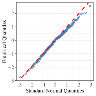
Figure 1: Q-Q plots for $\widehat{\theta}_{1}^{d}$ and $\widehat{\Delta}_{1}$ versus the standard normal distribution.

4.2 Performance of Algorithm 1 on Hypotheses Testing

We apply Algorithm 1 to concrete examples provided in Section 2.2. We select the tuning constant of $\lambda$ through cross-validation by letting $c=1$ for constructing the confidence intervals. We first evaluate the empirical coverage probability of the confidence interval $[\widehat{K}_{L},\widehat{K}_{U}]$. We set the nominal level at $0.95$, and set the sample size at $L\in\{5,50,100,150,250,300\}$ respectively. Figure 2 shows the empirical coverage probability at $K^{*}\in\{7,8,9,10,11,12\}$ for each setting of $L$. We can see that the empirical coverage probability of $[\widehat{K}_{L},\widehat{K}_{U}]$ converges to the nominal level of 0.95 as $L$ increases.

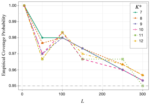
Figure 2: The empirical coverage probability of $[\widehat{K}_{L},\widehat{K}_{U}]$ constructed by Algorithm 1 at $L\in\{5,50,100,150,250,300\}$ when $K^{*}\in\{7,8,9,10,11,12\}$. The grey dashed line represents the nominal coverage probability equal to 0.95.

Then we provide two concrete examples. To characterize the distance of the alternative from the null, for a given set $S\subseteq[n]$, we define $d(K^{*},S)=\min_{i\in S}|i-K^{*}|$. Then for $K^{*}\notin\mathcal{K}_{0}$, $d(K^{*},\mathcal{K}_{0})$ characterizes the difficulty of differentiating ${\rm H}_{1}$ from ${\rm H}_{0}$. We summarize the results of Example 2 and Example 5 below.

Example 2

Recall that we are interested in testing whether a given set $A\subseteq[n]$ is a subset of the optimal set $\mathcal{S}^{*}$. In particular,

$$\mathrm{H}_{0}:A\nsubseteq\mathcal{S}^{*}\text{\leavevmode\nobreak\ versus\leavevmode\nobreak\ }\mathrm{H}_{1}:A\subseteq\mathcal{S}^{*}.$$

We set $A=\{2,4,6,8\}$ and generate $K^{*}\in\{7,8,9,10\}$. It can be seen that $\mathcal{K}_{0}=[7]$. We set the null at $K^{*}=7$ and choose different alternatives to evaluate the empirical Type I error and Power. The results are summarized in Figure 3. We see that the Type I error converges to the nominal 0.05 level as $L$ increases, while the Power increases to 1 as $L$ grows for all settings of $d(K^{*},\mathcal{K}_{0})$.

(a) Type I error	(b) Power

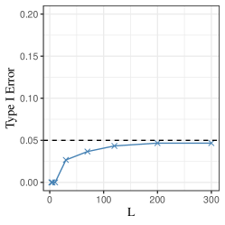
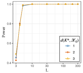
Figure 3: Type I error and Power for Example 2 under different $L$ and $d(K^{*},\mathcal{K}_{0})$, where the dashed line in (a) represents the nominal 0.05 level.

Example 5

Recall that for a partition $\{A_{1},\ldots,A_{m}\}$ of the products, i.e., $\bigcup_{j=1}^{m}A_{j}=[n]$ and $A_{j}\cap A_{k}=\varnothing$ for $j\neq k$, we are interested in testing if $A_{1}$ contains the most elements in $\mathcal{S}^{*}$ in comparison with the other $A_{j}$’s. In particular, we are interested in testing the hypothesis

$$\mathrm{H}_{0}:\lvert\mathcal{S}^{*}\cap A_{1}\rvert=\max_{j}\lvert\mathcal{S}^{*}\cap A_{j}\rvert\text{\leavevmode\nobreak\ versus\leavevmode\nobreak\ }\mathrm{H}_{1}:\lvert\mathcal{S}^{*}\cap A_{1}\rvert<\max_{j}\lvert\mathcal{S}^{*}\cap A_{j}\rvert.$$

For the simulation, we partition $[n]=[30]$ by $A_{1}=[6:8]\cup[14:15]\cup[21:25]$, $A_{2}=[1:3]\cup\{10,12\}\cup[16:20]$ and $A_{3}=[4:5]\cup\{9,11,13\}\cup[26:30]$, and the corresponding $\mathcal{K}_{0}$ is $[8:9]\cup\{15\}\cup[25:30]$. We generate $K^{*}\in\{9,10,11,12\}$ and set the null at $K^{*}=9$. Results are summarized in Figure 4. The Type I error converges to the nominal level of 0.05 as $L$ increases, while the Power increases to 1 as $L$ increases at $d(K^{*},\mathcal{K}_{0})\in\{1,2,3\}$.

(a) Type I error	(b) Power

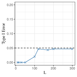
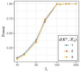
Figure 4: Type I error and Power for Example 5 under different $L$ and $d(K^{*},\mathcal{K}_{0})$, where the dashed line in (a) represents the nominal 0.05 level.

In summary, Algorithm 1 performs well for both examples, which shows the validity of our method.

5 Conclusion

To conclude, we propose a general inferential framework for testing combinatorial properties of the optimal assortment, which is the first paper making such efforts to the best of our knowledge. Under the MNL model, we first estimate the latent preference scores based on penalized likelihood optimization from customer choice data among selected offer sets. Then we apply a Newton debiasing correction to the estimator and perform the assortment optimization algorithm by plugging in the debiased latent score estimator. Finally, we implement the Gaussian multiplier bootstrap to construct confidence intervals for the optimal offer set and then perform hypothesis testing on a given property of interest upon the optimal assortment. We provide theoretical guarantees that our test is valid if the sample size is large enough under some mild conditions.

For future work, we plan to generalize the current results to other choice models, such as the capacitated MNL model with cardinality constraints, or the mixture of multinomial logit models (MMNL). We will also seek to develop a more computationally efficient and scalable method for constructing the confidence interval for $K^{*}$.

Supplementary Materials to

Combinatorial Inference on the Optimal Assortment in Multinomial Logit Models

Before starting with the proofs, we introduce some useful notations to be used later. Define $\mathcal{I}=\{S\subseteq[n]_{+}:S={\mathcal{S}}_{+},{\mathcal{S}}\in{\boldsymbol{\mathcal{S}}}\backslash\varnothing\}$ to be the set of all non-empty offered assortments augmented by the no-purchase option, where we denote ${\mathcal{S}}_{+}$ by $S$ for the convenience of notation. Define $\mathcal{I}_{k}=\{S\subseteq\mathcal{I}:|S|=k\}$ to be the subsets of $\mathcal{I}$ with cardinality equal to $k$, $2\leq k\leq n+1$. Correspondingly, we let $\boldsymbol{\mathcal{E}}_{k}=\{S\in\mathcal{I}_{k}:\mathcal{E}_{S}=1\}$ for $k=2,3,\ldots,n+1$. Denote by $\mathbb{I}\{\cdot\}$ an indicator function of statements, which is equal to 1 if the statement inside $\{\cdot\}$ holds true and 0 otherwise.

A Proof of Theorem 3.1

The proof basically modifies that of Theorem 6 in Chen et al., 2019b . Note that if we take $\boldsymbol{\theta}^{\prime}={\mathbf{P}}_{\mathbf{1}}^{\perp}\boldsymbol{\theta}$, then the convex problem (3.3) can be equivalently written as

$$\min_{\boldsymbol{\theta}^{\prime}\in\mathbb{R}^{n+1},\mathbf{1}^{\top}\boldsymbol{\theta}^{\prime}=0}\mathcal{L}_{\lambda}(\boldsymbol{\theta}^{\prime};\bm{x}):=\mathcal{L}(\boldsymbol{\theta}^{\prime};\bm{x})+\frac{\lambda}{2}\|\boldsymbol{\theta}^{\prime}\|_{2}^{2}.$$ (A.1)

Later we will show that the minimizer of $\mathcal{L}(\boldsymbol{\theta}^{\prime};\bm{x})+\frac{\lambda}{2}\|\boldsymbol{\theta}^{\prime}\|_{2}^{2}$ belongs to the subspace perpendicular to $\mathbf{1}$, and thus we can simplify (A.1) as

$$\min_{\boldsymbol{\theta}\in\mathbb{R}^{n+1}}\mathcal{L}_{\lambda}(\boldsymbol{\theta};\bm{x}):=\mathcal{L}(\boldsymbol{\theta};\bm{x})+\frac{\lambda}{2}\|\boldsymbol{\theta}\|_{2}^{2}.$$ (A.2)

It can be observed that the regularized MLE to (A.2) will be $\widehat{\boldsymbol{\theta}}^{\prime}:={\mathbf{P}}_{\mathbf{1}}^{\perp}\widehat{\boldsymbol{\theta}}$, where $\widehat{\boldsymbol{\theta}}$ is the regularized MLE of problem (3.3). In the following proof, we will consider solving (A.2) instead. We will show the $L_{2}$ convergence rate of the resulting MLE of (A.2), i.e., $\|\widehat{\boldsymbol{\theta}}^{\prime}-{\mathbf{P}}_{\mathbf{1}}^{\perp}\boldsymbol{\theta}^{*}\|_{2}=\|{\mathbf{P}}_{\mathbf{1}}^{\perp}\widehat{\boldsymbol{\theta}}-{\mathbf{P}}_{\mathbf{1}}^{\perp}\boldsymbol{\theta}^{*}\|_{2}$. Since $\widehat{\boldsymbol{\theta}}^{\prime}$ can be easily transformed back to $\widehat{\boldsymbol{\theta}}$ by taking $\widehat{\theta}_{i}=\widehat{\theta}_{i}^{\prime}-\widehat{\theta}^{\prime}_{0}$ for $i\in[n]_{+}$, the $L_{2}$ convergence rates $\|\widehat{\boldsymbol{\theta}}^{\prime}-{\mathbf{P}}_{\mathbf{1}}^{\perp}\boldsymbol{\theta}^{*}\|_{2}$ and $\|\widehat{\boldsymbol{\theta}}-\boldsymbol{\theta}^{*}\|_{2}$ will be different only by a factor of constant. Besides, since $\boldsymbol{\theta}^{*}$ and ${\mathbf{P}}_{\mathbf{1}}^{\perp}\boldsymbol{\theta}^{*}$ essentially specify the same MNL model, without loss of generality, we will replace $\boldsymbol{\theta}^{*}$ by ${\mathbf{P}}_{\mathbf{1}}^{\perp}\boldsymbol{\theta}^{*}$ throughout the proofs, and we will abuse the notation and let $\boldsymbol{\theta}^{*}$ denote $\boldsymbol{\theta}^{*\prime}={\mathbf{P}}_{\mathbf{1}}^{\perp}\boldsymbol{\theta}^{*}$ and let $\widehat{\boldsymbol{\theta}}$ denote $\widehat{\boldsymbol{\theta}}^{\prime}={\mathbf{P}}_{\mathbf{1}}^{\perp}\widehat{\boldsymbol{\theta}}$, i.e., the resulting regularized MLE solving problem (A.2). Before delving into the details, we need the following lemmas to help with the proof.

To study the gradient and Hessian for the log-likelihood, we define the auxiliary matrix

$$\mathbf{L}_{\boldsymbol{\mathcal{E}}}=\sum_{k=2}^{n+1}\sum_{S\in\boldsymbol{\mathcal{E}}_{k}}\bigg{\{}\frac{1}{k^{2}}\sum_{\begin{subarray}{c}i,j\in S\\ i<j\end{subarray}}(\boldsymbol{e}_{i}-\boldsymbol{e}_{j})(\boldsymbol{e}_{i}-\boldsymbol{e}_{j})^{\top}\bigg{\}}.$$

Since $\mathbf{L}_{\boldsymbol{\mathcal{E}}}$ is singular with columns perpendicular to $\mathbf{1}$, we define $\lambda_{\min,\perp}$ to be the smallest eigenvalue restricted to the eigenvectors orthogonal to $\mathbf{1}$. More specifically, for a symmetric matrix $\mathbf{M}$, we define

$$\lambda_{\min,\perp}(\mathbf{M})=\min\{\lambda:\mathbf{v}^{\top}\mathbf{M}\mathbf{v}\geq\lambda,\text{ for all }\mathbf{v}\text{ such that }\|\mathbf{v}\|_{2}=1\text{ and }\mathbf{v}^{\top}\mathbf{1}=0\}.$$

Then the following lemma characterizes the range of eigenvalues of $\mathbf{L}_{\boldsymbol{\mathcal{E}}}$.

Lemma A.1.

We define $M_{n}=\sum_{k=2}^{n+1}\frac{1}{k^{2}}{n-2\choose k-3}\asymp 2^{n}/n^{2}$ and $N_{n}=\sum_{k=2}^{n+1}\frac{1}{k^{2}}{n-1\choose k-2}\asymp 2^{n+1}/n^{2}$. Under the condition that $2^{n}p\geq Cn\log n$ for some large enough constant $C>0$, we have that the event

$$\mathcal{A}_{\mathbf{L}_{\boldsymbol{\mathcal{E}}}}:=\left\{\lambda_{\min,\perp}(\mathbf{L}_{\boldsymbol{\mathcal{E}}})\geq\frac{1}{2}(nM_{n}+N_{n})p,\quad\lambda_{\max}(\mathbf{L}_{\boldsymbol{\mathcal{E}}})\leq\frac{3}{2}(n+1)N_{n}p\right\}$$ (A.3)

holds with probability at least $1-O(n^{-10})$.

The proof of Lemma A.1 is deferred to Section F.1. Based upon Lemma A.1, the following lemmas depict the smoothness and convexity of the log-likelihood function,

Lemma A.2.

Under the same conditions as Lemma A.1, for all $\boldsymbol{\theta}\in\mathbb{R}^{n+1}$ such that $\|\boldsymbol{\theta}-\boldsymbol{\theta}^{*}\|_{\infty}\leq C$ for some $C\geq 0$, under the event $\mathcal{A}_{\mathbf{L}_{\boldsymbol{\mathcal{E}}}}$ defined in (A.3) we have

$$\lambda_{\min,\perp}\!\left(\nabla^{2}\mathcal{L}_{\lambda}(\boldsymbol{\theta};\bm{x})\!\right)\!\geq\!\lambda+\frac{1}{2(\kappa_{\boldsymbol{\theta}}e^{2C})^{2}}(nM_{n}+N_{n})p,\,\,\lambda_{\max}\!\left(\nabla^{2}\mathcal{L}_{\lambda}(\boldsymbol{\theta};\bm{x})\!\right)\!\leq\lambda+\frac{3(\kappa_{\boldsymbol{\theta}}e^{2C})^{2}}{2}(n+1)N_{n}p.$$ (A.4)

Please see Section F.2 for the proof of Lemma A.2.

Lemma A.3.

Under the same conditions as Lemma A.1 and the condition that $\lambda\asymp\sqrt{{nM_{n}p\log n}/{L}}$, the following event

$$\mathcal{A}_{g}:=\left\{\|\nabla\mathcal{L}_{\lambda}(\boldsymbol{\theta}^{*};\bm{x})\|_{2}\lesssim n\sqrt{\frac{M_{n}p\log n}{L}}\right\}$$ (A.5)

occurs with probability at least $1-O(n^{-10})$.

Please refer to Section F.3 for the proof of Lemma A.3.

Lemma A.4.

Under the same conditions as Lemma A.1, with probability at least $1-n^{-10}$, we have that for any $\boldsymbol{\theta}\in\mathbb{R}^{n+1}$ the following event holds

$$\mathcal{A}_{h}:=\left\{\|\nabla^{2}\mathcal{L}_{\lambda}(\boldsymbol{\theta};\bm{x})\|_{2}\leq\lambda+3(n+1)2^{n}p/16\right\}.$$ (A.6)

Please see Section F.4 for the proof of Lemma A.4. Now we begin with the proof. Same as Chen et al., 2019b did in their proof, we let $\boldsymbol{\theta}^{T}$ be the output of the following gradient descent

• Initialize $\boldsymbol{\theta}^{0}=\boldsymbol{\theta}^{*}$,

• for $t=0,1,\ldots,T-1$,

  $$\boldsymbol{\theta}^{t+1}=\boldsymbol{\theta}^{t}-\eta\nabla\mathcal{L}_{\lambda}(\boldsymbol{\theta}^{t};\bm{x}),$$

  where $\eta$ is taken to be $1/(\lambda+n2^{n}p/4)$.

Step I

By Lemma A.4, we know that with probability at least $1-n^{-10}$, $\mathcal{L}_{\lambda}(\boldsymbol{\theta};\bm{x})$ is $(\lambda+n2^{n}p/4)$-smooth and $\lambda$-strongly convex for any $\boldsymbol{\theta}\in\mathbb{R}^{n+1}$, then by Theorem 3.10 in Bubeck et al., (2015) we have

$$\|\boldsymbol{\theta}^{t}-\widehat{\boldsymbol{\theta}}\|_{2}\leq\rho^{t}\|\boldsymbol{\theta}^{*}-\widehat{\boldsymbol{\theta}}\|_{2},$$

where $\rho=1-\frac{\lambda}{\lambda+n2^{n}p/4}$. Note that since $\mathbf{1}^{\top}\bm{\theta}^{*}=0$ and $\mathbf{1}^{\top}\nabla\mathcal{L}(\boldsymbol{\theta};\bm{x})=\mathbf{0}$ for any $\boldsymbol{\theta}\in\mathbb{R}^{n+1}$, it follows by simple induction that $\mathbf{1}^{\top}\boldsymbol{\theta}^{t}=0$ for all $t\geq 1$, and hence $\widehat{\boldsymbol{\theta}}^{\top}\mathbf{1}=0$ due the convergence of $\boldsymbol{\theta}^{t}$ to $\widehat{\boldsymbol{\theta}}$. The following lemma provides an initial upper bound for $\|\boldsymbol{\theta}^{*}-\widehat{\boldsymbol{\theta}}\|_{2}$.

Lemma A.5.

On the event $\mathcal{A}_{g}$ as defined in (A.5), there exists a constant $c>0$ such that

$$\|\widehat{\boldsymbol{\theta}}-\boldsymbol{\theta}^{*}\|_{2}\leq c\sqrt{n}.$$

The proof is deferred to Section F.5. Recall that $\lambda\asymp\sqrt{\frac{2^{n}p\log n}{nL}}$, then with Lemma A.5, under the event $\mathcal{A}_{g}$, for large enough $T$ we have

$$\|\boldsymbol{\theta}^{T}-\widehat{\boldsymbol{\theta}}\|_{2} \leq\rho^{T}\|\widehat{\boldsymbol{\theta}}-\boldsymbol{\theta}^{*}\|_{2}\lesssim\left(1-\frac{\lambda}{\lambda+n2^{n}p/4}\right)^{T}\sqrt{n}$$

$$\leq\exp\left(-\frac{T\lambda}{\lambda+n2^{n}p/4}\right)\sqrt{n}\leq\exp\left(-c_{3}T\sqrt{\frac{\log n}{n^{3}2^{n}pL}}\right)\sqrt{n}$$

$$\lesssim\sqrt{\frac{\log n}{n2^{n}pL}}.$$

Step II

Now we show the convergence rate of $\|\boldsymbol{\theta}^{T}-\boldsymbol{\theta}^{*}\|_{2}$ by induction. More specifically, we propose that with probability at least $1-O(n^{-10})$, the following holds true for some constant $C_{1}>0$ for any $t\in[T]_{+}$,

$$\|\boldsymbol{\theta}^{t}-\boldsymbol{\theta}^{*}\|_{2}\leq C_{1}\sqrt{\frac{\log n}{M_{n}pL}}.$$ (A.7)

Note that the base case $t=0$ holds true trivially because of our setting of $\boldsymbol{\theta}^{0}=\boldsymbol{\theta}^{*}$. Now suppose that (A.7) holds true for the $t$-th iteration, we will show that under the event ${\boldsymbol{\mathcal{A}}}_{g}\cap{\boldsymbol{\mathcal{A}}}_{\mathbf{L}_{\boldsymbol{\mathcal{E}}}}$ (occurring with probability at least $1-O(n^{-10})$), the following holds

$$\|\boldsymbol{\theta}^{t+1}-\boldsymbol{\theta}^{*}\|_{2}\leq C_{1}\sqrt{\frac{\log n}{M_{n}pL}}.$$

First note that if (A.7) holds for the $t$-th iteration, we have

$$\|\boldsymbol{\theta}^{t}-\boldsymbol{\theta}^{*}\|_{\infty}\leq\|\boldsymbol{\theta}^{t}-\boldsymbol{\theta}^{*}\|_{2}\leq C_{1}\sqrt{\frac{\log n}{M_{n}pL}}.$$

The rest of the proof follows the proof of Lemma 14 in Chen et al., 2019b with modifications. From the gradient descent algorithm, we know that

$$\boldsymbol{\theta}^{t+1}-\boldsymbol{\theta}^{*} =\boldsymbol{\theta}^{t}-\eta\nabla\mathcal{L}_{\lambda}\left(\boldsymbol{\theta}^{t};\bm{x}\right)-\boldsymbol{\theta}^{*}$$

$$=\boldsymbol{\theta}^{t}-\eta\nabla\mathcal{L}_{\lambda}\left(\boldsymbol{\theta}^{t};\bm{x}\right)-\left[\boldsymbol{\theta}^{*}-\eta\nabla\mathcal{L}_{\lambda}\left(\boldsymbol{\theta}^{*};\bm{x}\right)\right]-\eta\nabla\mathcal{L}_{\lambda}\left(\boldsymbol{\theta}^{*};\bm{x}\right)$$

$$=\left\{\boldsymbol{I}_{n}-\eta\int_{0}^{1}\nabla^{2}\mathcal{L}_{\lambda}(\boldsymbol{\theta}(\tau);\bm{x})\mathrm{d}\tau\right\}\left(\boldsymbol{\theta}^{t}-\boldsymbol{\theta}^{*}\right)-\eta\nabla\mathcal{L}_{\lambda}\left(\boldsymbol{\theta}^{*};\bm{x}\right),$$

where $\boldsymbol{\theta}(\tau):=\boldsymbol{\theta}^{*}+\tau(\boldsymbol{\theta}^{t}-\boldsymbol{\theta}^{*})$. Then we can see that if $C_{1}\sqrt{{\log n}/{(M_{n}pL)}}\leq\epsilon$ for a sufficiently small constant $\epsilon$, we have that $\|\boldsymbol{\theta}(\tau)-\boldsymbol{\theta}^{*}\|_{\infty}\leq\tau\|\boldsymbol{\theta}^{t}-\boldsymbol{\theta}^{*}\|_{\infty}\leq\epsilon$. Then by Lemma A.2 we have that under event $\mathcal{A}_{\mathbf{L}_{\boldsymbol{\mathcal{E}}}}$ defined in (A.3) (which occurs with probability at least $1-O(n^{-10})$), for all $\tau\in[0,1]$

$$\lambda+\frac{1}{3\kappa_{\boldsymbol{\theta}}^{2}}nM_{n}p\leq\lambda_{\min,\perp}\left(\nabla^{2}\mathcal{L}_{\lambda}(\boldsymbol{\theta}(\tau);\bm{x})\right)\leq\lambda_{\max}\left(\nabla^{2}\mathcal{L}_{\lambda}(\boldsymbol{\theta}(\tau);\bm{x})\right)\leq\lambda+n2^{n}p/4.$$

Now we denote $\mathbf{B}=\int_{0}^{1}\nabla^{2}\mathcal{L}_{\lambda}(\boldsymbol{\theta}(\tau);\bm{x})\mathrm{d}\tau$, then we have

$$\mathbf{B}\mathbf{1}_{n+1} =\int_{0}^{1}\nabla^{2}\mathcal{L}_{\lambda}(\boldsymbol{\theta}(\tau);\bm{x})\mathbf{1}_{n+1}\mathrm{d}\tau=\mathbf{0};$$

$$\lambda_{\min,\perp}(\mathbf{B}) =\min_{\mathbf{v}\in{\mathbf{S}}^{n},\mathbf{v}^{\top}\mathbf{1}=0}\int_{0}^{1}\mathbf{v}^{\top}\nabla^{2}\mathcal{L}_{\lambda}(\boldsymbol{\theta}(\tau);\bm{x})\mathbf{v}\mathrm{d}\tau\geq\int_{0}^{1}\lambda_{\min,\perp}\left(\nabla^{2}\mathcal{L}_{\lambda}(\boldsymbol{\theta}(\tau);\bm{x})\right)\mathrm{d}\tau$$

$$\geq\lambda+\frac{1}{3\kappa_{\boldsymbol{\theta}}^{2}}nM_{n}p;$$

$$\lambda_{\max}(\mathbf{B}) =\max_{\mathbf{v}\in{\mathbf{S}}^{n}}\int_{0}^{1}\mathbf{v}^{\top}\nabla^{2}\mathcal{L}_{\lambda}(\boldsymbol{\theta}(\tau);\bm{x})\mathbf{v}\mathrm{d}\tau\leq\lambda+n2^{n}p/4.$$

Besides, by the definition of $\eta$ we have that $1-\eta\left(\lambda+\frac{1}{3\kappa_{\boldsymbol{\theta}}^{2}}nM_{n}p\right)\geq 1-\eta\left(\lambda+n2^{n}p/4\right)\geq 0$. Combining the above results we have

$$\|\boldsymbol{\theta}^{t+1}-\boldsymbol{\theta}^{*}\|_{2} \leq\left(1-\frac{1}{3\kappa_{\boldsymbol{\theta}}^{2}}\eta nM_{n}p\right)\|\boldsymbol{\theta}^{t}-\boldsymbol{\theta}^{*}\|_{2}+\eta\|\nabla\mathcal{L}_{\lambda}\left(\boldsymbol{\theta}^{*};\bm{x}\right)\|_{2}$$

$$\leq\left(1-\frac{1}{3\kappa_{\boldsymbol{\theta}}^{2}}\eta nM_{n}p\right)C_{1}\sqrt{\frac{\log n}{M_{n}pL}}+C\eta n\sqrt{\frac{M_{n}p\log n}{L}}$$

$$\leq C_{1}\sqrt{\frac{\log n}{M_{n}pL}},$$

so long as $C_{1}$ is large enough.

Step III

Combing the results in Step I and Step II, as $T$ goes to infinity we have that with probability at least $1-O(n^{-10})$,

$$\|\boldsymbol{\theta}^{T}-\boldsymbol{\theta}^{*}\|_{2}\lesssim\sqrt{\frac{\log n}{M_{n}pL}}\lesssim n\sqrt{\frac{\log n}{2^{n}pL}},$$

and

$$\|\widehat{\boldsymbol{\theta}}-\boldsymbol{\theta}^{*}\|_{2}\leq\|\boldsymbol{\theta}^{T}-\widehat{\boldsymbol{\theta}}\|_{2}+\|\boldsymbol{\theta}^{T}-\boldsymbol{\theta}^{*}\|_{2}\lesssim n\sqrt{\frac{\log n}{2^{n}pL}}.$$

B Proof of Theorem 3.2

Before we begin with the proof, we first propose the following lemmas that provide bounds for several terms to be used in the proof.

Lemma B.1.

Under the same conditions as Theorem 3.1, for any $\boldsymbol{\theta}\in\mathbb{R}^{n+1}$ such that $\|\boldsymbol{\theta}-\boldsymbol{\theta}^{*}\|_{\infty}<C$ for some constant $C>0$, with probability at least $1-O(n^{-10})$ we have the following bounds

$$\|\nabla\mathcal{L}(\boldsymbol{\theta}^{*};\bm{x})\|_{\infty}\lesssim\sqrt{\frac{nM_{n}p\log n}{L}},$$ (B.1)

$$\|\nabla\mathcal{L}(\widehat{\boldsymbol{\theta}};\bm{x})-\nabla\mathcal{L}(\boldsymbol{\theta}^{*};\bm{x})-\nabla^{2}\mathcal{L}(\boldsymbol{\theta}^{*};\bm{x})(\widehat{\boldsymbol{\theta}}-\boldsymbol{\theta}^{*})\|_{\infty}\lesssim\frac{n\log n}{L},$$ (B.2)

$$\|\nabla^{2}\mathcal{L}(\widehat{\boldsymbol{\theta}};\bm{x})-\nabla^{2}\mathcal{L}(\boldsymbol{\theta}^{*};\bm{x})\|_{\infty}\lesssim n\sqrt{\frac{M_{n}p\log n}{L}},$$ (B.3)

$$\left\|\begin{pmatrix}\nabla^{2}\mathcal{L}(\widehat{\boldsymbol{\theta}};\bm{x})&\mathbf{1}\\ \mathbf{1}^{\top}&0\end{pmatrix}^{-1}-\begin{pmatrix}\nabla^{2}\mathcal{L}(\boldsymbol{\theta}^{*};\bm{x})&\mathbf{1}\\ \mathbf{1}^{\top}&0\end{pmatrix}^{-1}\right\|_{2}\lesssim\frac{1}{\sqrt{n}M_{n}p}\sqrt{\frac{\log n}{M_{n}pL}}.$$ (B.4)

The proof of Lemma B.1 is deferred to Section F.6. The following corollary of Lemma B.1 helps characterize the Moore-Penrose inverse of the Hessian matrix.

Corollary B.2.

For any $\boldsymbol{\theta}\in\mathbb{R}^{n+1}$, we have that

$$\begin{pmatrix}\nabla^{2}\mathcal{L}(\boldsymbol{\theta};\bm{x})&\mathbf{1}\\ \mathbf{1}^{\top}&0\end{pmatrix}^{-1}=\begin{pmatrix}\nabla^{2}\mathcal{L}(\boldsymbol{\theta};\bm{x})^{\dagger}&\frac{1}{n+1}\mathbf{1}\\ \frac{1}{n+1}\mathbf{1}^{\top}&0\end{pmatrix}.$$

Besides, for $\boldsymbol{\theta}\in\mathbb{R}^{n+1}$ such that $\|\boldsymbol{\theta}-\boldsymbol{\theta}^{*}\|_{\infty}<C$ for some constant $C>0$, with probability at least $1-O(n^{-10})$ we have that $[\nabla^{2}\mathcal{L}(\boldsymbol{\theta};\bm{x})^{\dagger}]_{jj}\asymp\frac{1}{nM_{n}p}$ for $j\in[n+1]$ and $\big{|}[\nabla^{2}\mathcal{L}(\boldsymbol{\theta};\bm{x})^{\dagger}]_{jk}\big{|}\lesssim\frac{1}{nM_{n}p}$ for $j\neq k$.

See Section F.7 for the proof of Corollary B.2. The following lemma provides a decomposition of the error of the debiased MLE $\widehat{\boldsymbol{\theta}}^{d}$ into the leading term and the remainder term.

Lemma B.3.

Under the same conditions as Theorem 3.1 , we have the following decomposition for the debiased MLE

$$\widehat{\boldsymbol{\theta}}^{d}-\boldsymbol{\theta}^{*}=-\nabla^{2}\mathcal{L}(\boldsymbol{\theta}^{*};\bm{x})^{\dagger}\nabla\mathcal{L}(\boldsymbol{\theta}^{*};\bm{x})+\mathbf{R}_{0},$$ (B.5)

where the residual term

$$\|\mathbf{R}_{0}\|_{2}\lesssim\frac{\sqrt{n}\log n}{M_{n}pL}\left(\sqrt{\frac{n\log n}{M_{n}pL}}+1\right)\lesssim\frac{n^{5/2}\log n}{2^{n}pL}\left(\sqrt{\frac{n^{3}\log n}{2^{n}pL}}+1\right),$$

with probability at least $1-O(n^{-10})$.

See Section F.8 for the proof of Lemma B.3. Now we can begin with the proof. We abbreviate $\mathcal{L}(\boldsymbol{\theta};\bm{x})$ to $\mathcal{L}(\boldsymbol{\theta})$ for the convenience of notation in the following proof. For $k\in[n]$, we define the mapping $\mathbf{v}_{k}(\cdot):\mathbb{R}^{n+1}\rightarrow\mathbb{R}^{n+1}$

$$\mathbf{v}_{k}(\boldsymbol{\theta})=\Big{(}\underbrace{(0-r_{k})e^{\theta_{0}},(r_{1}-r_{k})e^{\theta_{1}},(r_{2}-r_{k})e^{\theta_{2}},\ldots,(r_{k-1}-r_{k})e^{\theta_{k-1}}}_{\text{first $k$ entries}},0,\ldots,0\Big{)}^{\top},$$

and for the convenience of notation we let $\mathbf{v}_{k}=\mathbf{v}_{k}(\boldsymbol{\theta}^{*})$. Define the function

$$g_{k}(\boldsymbol{\theta})=\sum_{i=1}^{k}r_{i}\exp(\theta_{i})-(\sum_{i=0}^{k}\exp(\theta_{i}))r_{k},$$

and we have $\nabla g(\boldsymbol{\theta})=\mathbf{v}_{k}(\boldsymbol{\theta})$ and $\nabla^{2}g(\boldsymbol{\theta})=\operatorname{diag}\big{(}\mathbf{v}_{k}(\boldsymbol{\theta})\big{)}$, where

$$\mathbf{v}_{k}(\boldsymbol{\theta})=\Big{(}\underbrace{(0-r_{k})e^{\theta_{0}},(r_{1}-r_{k})e^{\theta_{1}},(r_{2}-r_{k})e^{\theta_{2}},\ldots,(r_{k-1}-r_{k})e^{\theta_{k-1}}}_{\text{first $k$ entries}},0,\ldots,0\Big{)}^{\top}.$$

Then we have

$$\widehat{\Delta}_{k}-\Delta_{k} =g_{k}(\widehat{\boldsymbol{\theta}}^{d})-g_{k}(\boldsymbol{\theta}^{*})=\nabla g(\boldsymbol{\theta}^{*})^{\top}(\widehat{\boldsymbol{\theta}}^{d}-\boldsymbol{\theta}^{*})+\frac{1}{2}(\widehat{\boldsymbol{\theta}}^{d}-\boldsymbol{\theta}^{*})^{\top}\nabla^{2}g(\widetilde{\boldsymbol{\theta}})(\widehat{\boldsymbol{\theta}}^{d}-\boldsymbol{\theta}^{*})$$

$$=\mathbf{v}_{k}(\boldsymbol{\theta}^{*})^{\top}(-\nabla^{2}\mathcal{L}(\boldsymbol{\theta}^{*})^{\dagger}\nabla\mathcal{L}(\boldsymbol{\theta}^{*})+\mathbf{R}_{0})+r_{1},$$

where $\|\widetilde{\boldsymbol{\theta}}-\boldsymbol{\theta}^{*}\|_{2}\leq\|\widehat{\boldsymbol{\theta}}^{d}-\boldsymbol{\theta}^{*}\|_{2}$, $\|\mathbf{R}_{0}\|_{2}\lesssim\frac{\sqrt{n}\log n}{M_{n}pL}\left(\sqrt{\frac{n\log n}{M_{n}pL}}+1\right)$ with probability at least $1-O(n^{-10})$ from Lemma B.3 , and

$$|r_{1}|=\frac{1}{2}(\widehat{\boldsymbol{\theta}}^{d}-\boldsymbol{\theta}^{*})^{\top}\nabla^{2}g(\widetilde{\boldsymbol{\theta}})(\widehat{\boldsymbol{\theta}}^{d}-\boldsymbol{\theta}^{*})\lesssim\|\mathbf{v}_{k}\|_{\infty}\|\widehat{\boldsymbol{\theta}}^{d}-\boldsymbol{\theta}^{*}\|_{2}^{2}.$$

Note that from the proof of Lemma B.3 we can see that $\mathbf{R}_{0}^{\top}\mathbf{1}={0}$, and hence $|\mathbf{v}_{k}^{\top}\mathbf{R}_{0}|\leq\|\mathbf{R}_{0}\|_{2}\|{\mathbf{P}}_{\mathbf{1}}^{\perp}\mathbf{v}_{k}\|_{2}$, where ${\mathbf{P}}_{\mathbf{1}}^{\perp}$ is the projection matrix to the perpendicular space of $\mathbf{1}$. Also from Lemma B.1 and the proof of Lemma B.3, we know that under the condition that $L\gtrsim n^{3}\log n/(2^{n}p)$, with high probability we have

$$\|\widehat{\boldsymbol{\theta}}^{d}-\boldsymbol{\theta}^{*}\|_{2}\lesssim\frac{1}{nM_{n}p}\times n\sqrt{\frac{M_{n}p\log n}{L}}+\frac{\sqrt{n}\log n}{M_{n}pL}\lesssim\sqrt{\frac{\log n}{M_{n}pL}},$$

and thus we have $|r_{1}|\lesssim\log n\|\mathbf{v}_{k}\|_{\infty}/(M_{n}pL)$. Now we consider the term $\mathbf{v}_{k}^{\top}\nabla^{2}\mathcal{L}(\boldsymbol{\theta}^{*})^{\dagger}\nabla\mathcal{L}(\boldsymbol{\theta}^{*})$. We have

$$-\mathbf{v}_{k}^{\top}\nabla^{2}\mathcal{L}(\boldsymbol{\theta}^{*})^{\dagger}\nabla\mathcal{L}\left(\boldsymbol{\theta}^{*}\right) =\frac{1}{L}\mathbf{v}_{k}^{\top}\nabla^{2}\mathcal{L}(\boldsymbol{\theta}^{*})^{\dagger}\sum_{\ell=1}^{L}\sum_{k^{\prime}=2}^{n+1}\sum_{S\in\boldsymbol{\mathcal{E}}_{k^{\prime}}}\left\{\sum_{i\in S}\left(x_{S}^{(i,\ell)}-\frac{e^{\theta_{i}^{*}}}{\sum_{j\in S}e^{\theta_{j}^{*}}}\right)\boldsymbol{e}_{i}\right\}$$

$$=\frac{1}{L}\sum_{\ell=1}^{L}\sum_{k^{\prime}=2}^{n+1}\sum_{S\in\boldsymbol{\mathcal{E}}_{k^{\prime}}}y_{S}^{(\ell)},$$

where $y_{S}^{(\ell)}:=\mathbf{v}_{k}^{\top}\nabla^{2}\mathcal{L}(\boldsymbol{\theta}^{*})^{\dagger}\left\{\sum_{i\in S}\left(x_{S}^{(i,\ell)}-\frac{e^{\theta_{i}^{*}}}{\sum_{j\in S}e^{\theta_{j}^{*}}}\right)\boldsymbol{e}_{i}\right\}$ are independent for $\ell$ and $S$ conditional on $\mathcal{E}$. Then with high probability, we have

$$\operatorname{Var}\left(\sum_{k^{\prime}=2}^{n+1}\sum_{S\in\boldsymbol{\mathcal{E}}_{k^{\prime}}}y_{S}^{(\ell)}\right)=\mathbf{v}_{k}^{\top}\nabla^{2}\mathcal{L}(\boldsymbol{\theta}^{*})^{\dagger}\nabla^{2}\mathcal{L}(\boldsymbol{\theta}^{*})\nabla^{2}\mathcal{L}(\boldsymbol{\theta}^{*})^{\dagger}\mathbf{v}_{k}=\mathbf{v}_{k}^{\top}\nabla^{2}\mathcal{L}(\boldsymbol{\theta}^{*})^{\dagger}\mathbf{v}_{k}\gtrsim\frac{\|{\mathbf{P}}_{\mathbf{1}}^{\perp}\mathbf{v}_{k}\|_{2}^{2}}{nM_{n}p}.$$

Now consider $\left|y_{S}^{(\ell)}\right|$, and with high probability we have

$$\left|y_{S}^{(\ell)}\right| \lesssim\sum_{i\in S}\left|x_{S}^{(i,\ell)}-\frac{e^{\theta_{i}^{*}}}{\sum_{j\in S}e^{\theta_{j}^{*}}}\right||\mathbf{v}_{k}^{\top}[\nabla^{2}\mathcal{L}(\boldsymbol{\theta}^{*})^{\dagger}]_{i}|\lesssim\frac{|S|}{nM_{n}p}\|{\mathbf{P}}_{\mathbf{1}}^{\perp}\mathbf{v}_{k}\|_{2},$$

where the last inequality is due to the fact that $\nabla^{2}\mathcal{L}(\boldsymbol{\theta}^{*})^{\dagger}\mathbf{1}=\mathbf{0}$. Then in turn we also have

$$\sum_{k^{\prime}=2}^{n+1}\sum_{S\in\boldsymbol{\mathcal{E}}_{k^{\prime}}}\mathbb{E}\left|y_{S}^{(\ell)}\right|^{3}\lesssim\left(\max_{S}\left|y_{S}^{(\ell)}\right|\right)\sum_{k^{\prime}=2}^{n+1}\sum_{S\in\boldsymbol{\mathcal{E}}_{k^{\prime}}}\mathbb{E}\left|y_{S}^{(\ell)}\right|^{2}\lesssim\frac{1}{M_{n}p}\mathbf{v}_{k}^{\top}\nabla^{2}\mathcal{L}(\boldsymbol{\theta}^{*})^{\dagger}\mathbf{v}_{k}\|{\mathbf{P}}_{\mathbf{1}}^{\perp}\mathbf{v}_{k}\|_{2}.$$

Thus under the condition that $n/\sqrt{M_{n}pL}=o(1)$, we have

$$\max_{k}\left(\sum_{\ell=1}^{L}\sum_{k^{\prime}=2}^{n+1}\sum_{S\in\boldsymbol{\mathcal{E}}_{k^{\prime}}}\operatorname{Var}\left(y_{S}^{(\ell)}\right)\right)^{-3/2}\left(\sum_{\ell=1}^{L}\sum_{k^{\prime}=2}^{n+1}\sum_{S\in\boldsymbol{\mathcal{E}}_{k^{\prime}}}\mathbb{E}\left|y_{S}^{(\ell)}\right|^{3}\right)=o(1).$$

Then by Lyapunov’s Central Limit Theorem, we have

$$\sqrt{L}(\mathbf{v}_{k}^{\top}\nabla^{2}\mathcal{L}(\boldsymbol{\theta}^{*})^{\dagger}\mathbf{v}_{k})^{-1/2}\left(\mathbf{v}_{k}^{\top}\nabla^{2}\mathcal{L}(\boldsymbol{\theta}^{*})^{\dagger}\nabla\mathcal{L}(\boldsymbol{\theta}^{*})\right)\big{|}\,\mathcal{E}\overset{d}{\rightarrow}N(0,1),\text{ for all }k\in[n].$$

Besides, under the condition that

$$\max_{k}\left\{\frac{{n}\log n}{\sqrt{M_{n}pL}}+\frac{\log n\|\mathbf{v}_{k}\|_{\infty}}{\|{\mathbf{P}}_{\mathbf{1}}^{\perp}\mathbf{v}_{k}\|_{2}}\sqrt{\frac{n}{M_{n}pL}}\right\}=o(1),$$ (B.6)

we have $\sqrt{L}(\mathbf{v}_{k}^{\top}\nabla^{2}\mathcal{L}(\boldsymbol{\theta}^{*})^{\dagger}\mathbf{v}_{k})^{-1/2}(\mathbf{v}_{k}^{\top}\mathbf{R}_{0}+r_{1})=o_{P}(1)$, and by Slutsky’s Theorem the claim follows.

Now to simplify the conditions, we turn to study the norm $\|{\mathbf{P}}_{\mathbf{1}}^{\perp}\mathbf{v}_{k}\|_{2}$ for $k\in[n]$. First note that ${\mathbf{P}}_{\mathbf{1}}\mathbf{v}_{k}=(n+1)^{-1}\Delta_{k}\cdot\mathbf{1}$. Due to the non-decreasingness of $\Delta_{k}$, we consider the scenarios of $k\leq K^{*}$ and $k>K^{*}$ separately.

• $k\leq K^{*}$. From Theorem 2.1 we know that $\Delta_{k}\leq 0$ when $k\leq K^{*}$. Besides, since $(r_{i}-r_{k})u_{i}^{*}\geq 0$ for $i<k$, we know that $|r_{k}u_{0}^{*}|\geq|\Delta_{k}|$. Thus we have that

  $$\|{\mathbf{P}}_{\mathbf{1}}^{\perp}\mathbf{v}_{k}\|_{2}^{2} =\left(-r_{k}u_{0}^{*}-\frac{\Delta_{k}}{n+1}\right)^{2}+\sum_{i=1}^{k-1}\left\{(r_{i}-r_{k})u_{i}^{*}-\frac{\Delta_{k}}{n+1}\right\}^{2}+\frac{n-k+1}{(n+1)^{2}}\Delta_{k}^{2}$$

  $$=(r_{k}u_{0}^{*})^{2}+\sum_{i=1}^{k-1}\left((r_{i}-r_{k})u_{i}^{*}\right)^{2}-\frac{\Delta_{k}^{2}}{n+1}\geq(r_{k}u_{0}^{*})^{2}-\frac{\Delta_{k}^{2}}{n+1}$$

  $$\geq(r_{k}u_{0}^{*})^{2}-\frac{(r_{k}u_{0}^{*})^{2}}{n+1}=\frac{n}{n+1}(r_{k}u_{0}^{*})^{2}\geq\frac{(r_{k}u_{0}^{*})^{2}}{2}.$$

• $k>K^{*}$. When $k>K^{*}$, we know that $\Delta_{K}\geq 0$ from Theorem 2.1. Then we have

  $$\|{\mathbf{P}}_{\mathbf{1}}^{\perp}\mathbf{v}_{k}\|_{2}^{2} =\left(-r_{k}u_{0}^{*}-\frac{\Delta_{k}}{n+1}\right)^{2}+\sum_{i=1}^{k-1}\left\{(r_{i}-r_{k})u_{i}^{*}-\frac{\Delta_{k}}{n+1}\right\}^{2}+\frac{n-k+1}{(n+1)^{2}}\Delta_{k}^{2}$$

  $$\geq\left(-r_{k}u_{0}^{*}-\frac{\Delta_{k}}{n+1}\right)^{2}\geq(r_{n}u_{0}^{*})^{2}.$$

Combining the above results we have that $\|{\mathbf{P}}_{\mathbf{1}}^{\perp}\mathbf{v}_{k}\|_{2}\gtrsim r_{n}u_{0}^{*}$, and in turn we have that

$$\max_{k}\frac{\|\mathbf{v}_{k}\|_{\infty}}{\|{\mathbf{P}}_{\mathbf{1}}^{\perp}\mathbf{v}_{k}\|_{2}} \lesssim\frac{r_{1}\max_{i}u_{i}^{*}}{r_{n}u_{0}^{*}}\leq\kappa_{\boldsymbol{\theta}}\frac{r_{1}}{r_{n}}=\kappa_{r}\kappa_{\boldsymbol{\theta}}\lesssim\kappa_{r}.$$

Therefore, under the condition that $\kappa_{r}\lesssim\sqrt{n}$, the condition (B.6) simplifies to

$$\frac{{n}\log n}{\sqrt{M_{n}pL}}+\kappa_{r}\log n\sqrt{\frac{n}{M_{n}pL}}\lesssim\frac{{n}\log n}{\sqrt{M_{n}pL}}\lesssim\frac{n^{2}\log n}{\sqrt{2^{n}pL}}=o(1).$$

C Proof of Corollary 3.3

By Slutsky’s Theorem, it suffices for us to show that

$$\max_{k}\left\{\lvert\widehat{\mathbf{v}}_{k}^{\top}\nabla^{2}\mathcal{L}(\widehat{\boldsymbol{\theta}};\bm{x})^{\dagger}\widehat{\mathbf{v}}_{k}-\mathbf{v}_{k}^{\top}\nabla^{2}\mathcal{L}(\boldsymbol{\theta}^{*};\bm{x})^{\dagger}\mathbf{v}_{k}\rvert/\mathbf{v}_{k}^{\top}\nabla^{2}\mathcal{L}(\boldsymbol{\theta}^{*};\bm{x})^{\dagger}\mathbf{v}_{k}\right\}=o_{P}(1).$$

From (B.4), we know that $\|\nabla^{2}\mathcal{L}(\widehat{\boldsymbol{\theta}};\bm{x})^{\dagger}-\nabla^{2}\mathcal{L}(\boldsymbol{\theta}^{*};\bm{x})^{\dagger}\|_{2}\lesssim\frac{1}{\sqrt{n}M_{n}p}\sqrt{\frac{\log n}{M_{n}pL}}$ with high probability. Also from Theorem 3.1, we know that $\|\widehat{\boldsymbol{\theta}}-\boldsymbol{\theta}^{*}\|_{2}\lesssim\sqrt{\frac{\log n}{M_{n}pL}}$, and in turn

$$\|\widehat{\mathbf{v}}_{k}-\mathbf{v}_{k}\|_{2}=O_{P}\Big{(}\|\nabla^{2}g(\boldsymbol{\theta}^{*})(\widehat{\boldsymbol{\theta}}-\boldsymbol{\theta}^{*})\|_{2}\Big{)}=O_{P}\Big{(}\|\operatorname{diag}(\mathbf{v}_{k})\|_{2}\|\widehat{\boldsymbol{\theta}}-\boldsymbol{\theta}^{*}\|_{2}\Big{)}=O_{P}\left(\|\mathbf{v}_{k}\|_{\infty}\sqrt{\frac{\log n}{M_{n}pL}}\right).$$

Combining the previous results, we have

$$\lvert\widehat{\mathbf{v}}_{k}^{\top}\nabla^{2}\mathcal{L}(\widehat{\boldsymbol{\theta}};\bm{x})^{\dagger}\widehat{\mathbf{v}}_{k}-\mathbf{v}_{k}^{\top}\nabla^{2}\mathcal{L}(\boldsymbol{\theta}^{*};\bm{x})^{\dagger}\mathbf{v}_{k}\rvert\leq\lvert\widehat{\mathbf{v}}_{k}^{\top}(\nabla^{2}\mathcal{L}(\widehat{\boldsymbol{\theta}};\bm{x})^{\dagger}-\nabla^{2}\mathcal{L}(\boldsymbol{\theta}^{*};\bm{x})^{\dagger})\widehat{\mathbf{v}}_{k}\rvert$$

$$\quad+\lvert(\widehat{\mathbf{v}}_{k}-\mathbf{v}_{k})\nabla^{2}\mathcal{L}(\boldsymbol{\theta}^{*};\bm{x})^{\dagger}\mathbf{v}_{k}\rvert+\lvert(\widehat{\mathbf{v}}_{k}-\mathbf{v}_{k})\nabla^{2}\mathcal{L}(\boldsymbol{\theta}^{*};\bm{x})^{\dagger}\widehat{\mathbf{v}}_{k}\rvert$$

$$\quad=O_{P}\Big{(}\|\nabla^{2}\mathcal{L}(\widehat{\boldsymbol{\theta}};\bm{x})^{\dagger}-\nabla^{2}\mathcal{L}(\boldsymbol{\theta}^{*};\bm{x})^{\dagger}\|_{2}\|{\mathbf{P}}_{\mathbf{1}}^{\perp}\mathbf{v}_{k}\|_{2}^{2}+\|{\mathbf{P}}_{\mathbf{1}}^{\perp}\mathbf{v}_{k}\|_{2}\|\nabla^{2}\mathcal{L}(\boldsymbol{\theta}^{*};\bm{x})^{\dagger}\|_{2}\|\widehat{\mathbf{v}}_{k}-\mathbf{v}_{k}\|_{2}\Big{)}$$

$$\quad\lesssim\frac{\|{\mathbf{P}}_{\mathbf{1}}^{\perp}\mathbf{v}_{k}\|_{2}^{2}}{\sqrt{n}M_{n}p}\sqrt{\frac{\log n}{M_{n}pL}}+\frac{\|{\mathbf{P}}_{\mathbf{1}}^{\perp}\mathbf{v}_{k}\|_{2}\|\mathbf{v}_{k}\|_{\infty}}{nM_{n}p}\sqrt{\frac{\log n}{M_{n}pL}}.$$

Recall from the proof of Theorem 3.2 that $\mathbf{v}_{k}^{\top}\nabla^{2}\mathcal{L}(\boldsymbol{\theta}^{*};\bm{x})^{\dagger}\mathbf{v}_{k}\gtrsim\|{\mathbf{P}}_{\mathbf{1}}^{\perp}\mathbf{v}_{k}\|_{2}^{2}/(nM_{n}p)$, then under the condition that $\kappa_{r}\lesssim\sqrt{n}$ and $\sqrt{{n^{3}\log n}/{(2^{n}pL)}}=o(1)$, we have that with high probability

$$\max_{k}\left\{\frac{\lvert\widehat{\mathbf{v}}_{k}^{\top}\nabla^{2}\mathcal{L}(\widehat{\boldsymbol{\theta}};\bm{x})^{\dagger}\widehat{\mathbf{v}}_{k}-\mathbf{v}_{k}^{\top}\nabla^{2}\mathcal{L}(\boldsymbol{\theta}^{*};\bm{x})^{\dagger}\mathbf{v}_{k}\rvert}{\mathbf{v}_{k}^{\top}\nabla^{2}\mathcal{L}(\boldsymbol{\theta}^{*};\bm{x})^{\dagger}\mathbf{v}_{k}}\right\}$$

$$\lesssim\max_{k}\left\{\frac{\|{\mathbf{P}}_{\mathbf{1}}^{\perp}\mathbf{v}_{k}\|_{2}^{2}}{\sqrt{n}M_{n}p}\sqrt{\frac{\log n}{M_{n}pL}}\!+\!\frac{\|{\mathbf{P}}_{\mathbf{1}}^{\perp}\mathbf{v}_{k}\|_{2}\|\mathbf{v}_{k}\|_{\infty}}{nM_{n}p}\sqrt{\frac{\log n}{M_{n}pL}}\right\}\!\!\frac{nM_{n}p}{\|{\mathbf{P}}_{\mathbf{1}}^{\perp}\mathbf{v}_{k}\|_{2}^{2}}$$

$$=\max_{k}\left\{\sqrt{\frac{n\log n}{M_{n}pL}}+\frac{\|\mathbf{v}_{k}\|_{\infty}}{\|{\mathbf{P}}_{\mathbf{1}}^{\perp}\mathbf{v}_{k}\|_{2}}\sqrt{\frac{\log n}{M_{n}pL}}\right\}\lesssim\sqrt{\frac{n\log n}{M_{n}pL}}+\kappa_{r}\sqrt{\frac{\log n}{M_{n}pL}}\lesssim\sqrt{\frac{n^{3}\log n}{2^{n}pL}}=o(1),$$

and by Slutsky’s theorem, the claim follows.

D Proof of Lemma 3.5

In the following proof, we denote $\mathcal{L}(\boldsymbol{\theta};\bm{x})$ by $\mathcal{L}(\boldsymbol{\theta})$ for the convenience of notation. We will first show that with high probability with respect to $\boldsymbol{\mathcal{E}}$, the following event holds

$${\boldsymbol{\mathcal{A}}}_{\boldsymbol{\mathcal{E}}}:=\left\{\sup_{\boldsymbol{\theta}^{*}\in\mathbf{\Theta}}\sup_{\alpha\in(0,1)}\left|\mathbb{P}_{\boldsymbol{\theta}^{*}}\left(T>c_{W}(\alpha,\boldsymbol{\mathcal{E}})\,|\,\boldsymbol{\mathcal{E}}\right)-\alpha\right|=o(1)\right\}.$$ (D.1)

For the convenience of notation, for two positive sequences $x_{n}$ and $y_{n}$, we use $x_{n}\lesssim y_{n}$ or $x_{n}=O(y_{n})$ to imply that there exists a constant $C>0$ independent of $\boldsymbol{\theta}^{*}$ such that $x_{n}\leq Cy_{n}$ for large enough $n$.

For a given $\boldsymbol{\theta}^{*}\in\mathbf{\Theta}$, we define the following two auxiliary statistics,

$$T_{0}:=\max_{k\in[n]}\sum_{\ell=1}^{L}\left\{\frac{\mathbf{v}_{k}^{\top}\nabla^{2}\mathcal{L}(\boldsymbol{\theta}^{*})^{\dagger}}{\sqrt{L\mathbf{v}_{k}^{\top}\nabla^{2}\mathcal{L}(\boldsymbol{\theta}^{*})^{\dagger}\mathbf{v}_{k}}}\sum_{S\in\mathcal{I}}\mathcal{E}_{S}\left\{\sum_{i\in S}\left(x_{S}^{(i,\ell)}-\frac{e^{\theta_{i}^{*}}}{\sum_{j\in S}e^{\theta_{j}^{*}}}\right)\boldsymbol{e}_{i}\right\}\right\},$$ (D.2)

and

$$W_{0}:=\max_{k\in[n]}\sum_{\ell=1}^{L}\left\{\frac{\mathbf{v}_{k}^{\top}\nabla^{2}\mathcal{L}(\boldsymbol{\theta}^{*})^{\dagger}}{\sqrt{L\mathbf{v}_{k}^{\top}\nabla^{2}\mathcal{L}(\boldsymbol{\theta}^{*})^{\dagger}\mathbf{v}_{k}}}\sum_{S\in\boldsymbol{\mathcal{E}}}\left\{\sum_{i\in S}\left(x_{S}^{(i,\ell)}-\frac{e^{\theta_{i}^{*}}}{\sum_{j\in S}e^{\theta_{j}^{*}}}\right)\boldsymbol{e}_{i}\right\}z_{S,\ell}\right\}.$$ (D.3)

We define $y_{k}^{(\ell,S)}=\sqrt{\frac{|\boldsymbol{\mathcal{E}}|}{\mathbf{v}_{k}^{\top}\nabla^{2}\mathcal{L}(\boldsymbol{\theta}^{*})^{\dagger}\mathbf{v}_{k}}}\mathbf{v}_{k}^{\top}\nabla^{2}\mathcal{L}(\boldsymbol{\theta}^{*})^{\dagger}\left\{\sum_{i\in S}\left(x_{S}^{(i,\ell)}-\frac{e^{\theta_{i}^{*}}}{\sum_{j\in S}e^{\theta_{j}^{*}}}\right)\boldsymbol{e}_{i}\right\},\ell=1,\ldots,L,k=1,\ldots,n$. Then $W_{0}=\max_{k\in[n]}\frac{1}{\sqrt{L|\boldsymbol{\mathcal{E}}|}}\sum_{\ell=1}^{L}\sum_{S\in\boldsymbol{\mathcal{E}}}y_{k}^{(\ell,S)}z_{S,\ell}$. We will show that the following three conditions hold with high probability uniformly for all $\boldsymbol{\theta}^{*}\in\mathbf{\Theta}$.

1. There exist $\zeta_{1}$ and $\zeta_{2}$ independent of $\boldsymbol{\theta}^{*}$ with $\zeta_{1}\sqrt{\log n}+\zeta_{2}=o(1)$ such that $\mathbb{P}\left(\lvert T-T_{0}\rvert>\zeta_{1}\right)<\zeta_{2}$, $\mathbb{P}\left(\mathbb{P}\left(\lvert W-W_{0}\rvert>\zeta_{1}\,|\,\boldsymbol{x}\right)>\zeta_{2}\right)<\zeta_{2}$,

2. $c\leqslant\min_{k\in[n]}\frac{1}{L|\boldsymbol{\mathcal{E}}|}\sum_{\ell=1}^{L}\sum_{S\in\boldsymbol{\mathcal{E}}}\mathbb{E}[(y_{k}^{(\ell,S)})^{2}]$ for some constant $c>0$,

3. $\max_{k\in[n]}\lvert y_{k}^{(\ell,S)}\rvert\lesssim B$ with $B^{2}(\log(nL|\boldsymbol{\mathcal{E}}|))^{7}/(L|\boldsymbol{\mathcal{E}}|)=o(1)$ where $B$ is not necessarily a constant.

We first verify condition (2). For any $k\in[n]$, since $y_{k}^{(\ell,S)}$’s are independent conditional on $\mathcal{E}$, we have

$$\frac{1}{|\boldsymbol{\mathcal{E}}|L}\sum_{\ell=1}^{L}\sum_{S\in\boldsymbol{\mathcal{E}}}\mathbb{E}\big{[}(y_{k}^{(\ell,S)})^{2}\big{]} =\frac{1}{{{L\mathbf{v}_{k}^{\top}\nabla^{2}\mathcal{L}(\boldsymbol{\theta}^{*})^{\dagger}\mathbf{v}_{k}}}}\!\operatorname{Var}\!\left[\sum_{\ell=1}^{L}\!\left\{\!{\mathbf{v}_{k}^{\top}\nabla^{2}\mathcal{L}(\boldsymbol{\theta}^{*})^{\dagger}}\sum_{S\in\boldsymbol{\mathcal{E}}}\!\sum_{i\in S}\!\!\left(\!\!x_{S}^{(i,\ell)}\!-\frac{e^{\theta_{i}^{*}}}{\sum_{j\in S}e^{\theta_{j}^{*}}}\right)\!\!\boldsymbol{e}_{i}\!\right\}\!\right]$$

$$=\frac{\mathbf{v}_{k}^{\top}\nabla^{2}\mathcal{L}(\boldsymbol{\theta}^{*})^{\dagger}\mathbf{v}_{k}}{\mathbf{v}_{k}^{\top}\nabla^{2}\mathcal{L}(\boldsymbol{\theta}^{*})^{\dagger}\mathbf{v}_{k}}=1,$$

and thus condition (2) holds trivially. As for condition (3), with probability at least $1-O(n^{-10})$ we have

$$\left|y_{k}^{(\ell,S)}\right| =\sqrt{\frac{|\boldsymbol{\mathcal{E}}|}{\mathbf{v}_{k}^{\top}\nabla^{2}\mathcal{L}(\boldsymbol{\theta}^{*})^{\dagger}\mathbf{v}_{k}}}\left|\mathbf{v}_{k}^{\top}\nabla^{2}\mathcal{L}(\boldsymbol{\theta}^{*})^{\dagger}\left\{\sum_{i\in S}\left(x_{S}^{(i,\ell)}-\frac{e^{\theta_{i}^{*}}}{\sum_{j\in S}e^{\theta_{j}^{*}}}\right)\boldsymbol{e}_{i}\right\}\right|$$

$$=\sqrt{\frac{|\boldsymbol{\mathcal{E}}|}{\mathbf{v}_{k}^{\top}\nabla^{2}\mathcal{L}(\boldsymbol{\theta}^{*})^{\dagger}\mathbf{v}_{k}}}\left|({\mathbf{P}}_{\mathbf{1}}^{\perp}\mathbf{v}_{k})^{\top}\nabla^{2}\mathcal{L}(\boldsymbol{\theta}^{*})^{\dagger}\left\{\sum_{i\in S}x_{S}^{(i,\ell)}\boldsymbol{e}_{i}-\sum_{i\in S}\frac{e^{\theta_{i}^{*}}}{\sum_{j\in S}e^{\theta_{j}^{*}}}\boldsymbol{e}_{i}\right\}\right|$$

$$\lesssim\frac{\sqrt{n^{2}M_{n}p}}{\|{\mathbf{P}}_{\mathbf{1}}^{\perp}\mathbf{v}_{k}\|_{2}/\sqrt{nM_{n}p}}\|{\mathbf{P}}_{\mathbf{1}}^{\perp}\mathbf{v}_{k}\|_{2}\left\|\sum_{i\in S}x_{S}^{(i,\ell)}[\nabla^{2}\mathcal{L}(\boldsymbol{\theta}^{*})^{\dagger}]_{i}-\sum_{i\in S}\frac{e^{\theta_{i}^{*}}}{\sum_{j\in S}e^{\theta_{j}^{*}}}[\nabla^{2}\mathcal{L}(\boldsymbol{\theta}^{*})^{\dagger}]_{i}\right\|_{2}$$

$$\lesssim\sqrt{n}nM_{n}p\|\nabla^{2}\mathcal{L}(\boldsymbol{\theta}^{*})^{\dagger}\|_{2,\infty}\leq\sqrt{n}nM_{n}p\|\nabla^{2}\mathcal{L}(\boldsymbol{\theta}^{*})^{\dagger}\|_{2}\lesssim\sqrt{n},$$

where the last but two inequality is due to the fact that

$$\left\|\sum_{i\in S}x_{S}^{(i,\ell)}[\nabla^{2}\mathcal{L}(\boldsymbol{\theta}^{*})^{\dagger}]_{i}-\sum_{i\in S}\frac{e^{\theta_{i}^{*}}}{\sum_{j\in S}e^{\theta_{j}^{*}}}[\nabla^{2}\mathcal{L}(\boldsymbol{\theta}^{*})^{\dagger}]_{i}\right\|_{2}$$

$$\leq\sum_{i\in S}x_{S}^{(i,\ell)}\|[\nabla^{2}\mathcal{L}(\boldsymbol{\theta}^{*})^{\dagger}]_{i}\|_{2}+\sum_{i\in S}\frac{e^{\theta_{i}^{*}}}{\sum_{j\in S}e^{\theta_{j}^{*}}}\|[\nabla^{2}\mathcal{L}(\boldsymbol{\theta}^{*})^{\dagger}]_{i}\|_{2}$$

$$\leq\left(\sum_{i\in S}x_{S}^{(i,\ell)}+\sum_{i\in S}\frac{e^{\theta_{i}^{*}}}{\sum_{j\in S}e^{\theta_{j}^{*}}}\right)\|\nabla^{2}\mathcal{L}(\boldsymbol{\theta}^{*})^{\dagger}\|_{2,\infty}\leq 2\|\nabla^{2}\mathcal{L}(\boldsymbol{\theta}^{*})^{\dagger}\|_{2,\infty},$$

and from Lemma A.2, we know that $\sup_{\boldsymbol{\theta}^{*}\in\mathbf{\Theta}}\|\nabla^{2}\mathcal{L}(\boldsymbol{\theta}^{*})^{\dagger}\|_{2}\lesssim(nM_{n}p)^{-1}$ under the condition that $\sup_{\boldsymbol{\theta}^{*}\in\mathbf{\Theta}}\kappa_{\boldsymbol{\theta}^{*}}=O(1)$. Thus we can take $B=\sqrt{n}$, and condition (3) holds uniformly for $\boldsymbol{\theta}^{*}\in\mathbf{\Theta}$ under the condition that $n\big{(}\log(n2^{n}pL)\big{)}^{7}/(2^{n}pL)=o(1)$.

Now we move on to verify condition (1). First recall from previous proof that the following hold with probability at least $1-O(n^{-10})$,

$$\|\widehat{\boldsymbol{\theta}}^{d}-\boldsymbol{\theta}^{*}\|_{2}\lesssim\sqrt{\frac{\log n}{M_{n}pL}},\quad\|\widehat{\mathbf{v}}_{k}-\mathbf{v}_{k}\|_{2}\lesssim\|\mathbf{v}_{k}\|_{\infty}\sqrt{\frac{\log n}{M_{n}pL}},$$

$$\|\nabla\mathcal{L}(\widehat{\boldsymbol{\theta}})-\nabla\mathcal{L}(\boldsymbol{\theta}^{*})\|_{\infty}\lesssim n\sqrt{\frac{M_{n}p\log n}{L}},\quad\|\nabla^{2}\mathcal{L}(\widehat{\boldsymbol{\theta}})^{\dagger}-\nabla^{2}\mathcal{L}(\boldsymbol{\theta}^{*})^{\dagger}\|_{2}\lesssim\frac{1}{\sqrt{n}M_{n}p}\sqrt{\frac{\log n}{M_{n}pL}},$$

$$\left|\widehat{\mathbf{v}}_{k}^{\top}\nabla^{2}\mathcal{L}(\widehat{\boldsymbol{\theta}})^{\dagger}\widehat{\mathbf{v}}_{k}-\mathbf{v}_{k}^{\top}\nabla^{2}\mathcal{L}(\boldsymbol{\theta}^{*})^{\dagger}\mathbf{v}_{k}\right|\lesssim\frac{\|{\mathbf{P}}_{\mathbf{1}}^{\perp}\mathbf{v}_{k}\|_{2}^{2}}{\sqrt{n}M_{n}p}\sqrt{\frac{\log n}{M_{n}pL}}+\frac{\|{\mathbf{P}}_{\mathbf{1}}^{\perp}\mathbf{v}_{k}\|_{2}\|\mathbf{v}_{k}\|_{\infty}}{nM_{n}p}\sqrt{\frac{\log n}{M_{n}pL}}.$$

And based on the above upper bounds we have

$$\bigg{\lvert}\frac{1}{\sqrt{\widehat{\mathbf{v}}_{k}^{\top}\nabla^{2}\mathcal{L}(\widehat{\boldsymbol{\theta}})^{\dagger}\widehat{\mathbf{v}}_{k}}}\!-\!\frac{1}{\sqrt{\mathbf{v}_{k}^{\top}\nabla^{2}\mathcal{L}(\boldsymbol{\theta}^{*})^{\dagger}\mathbf{v}_{k}}}\bigg{\rvert}\!\lesssim\!\frac{1}{\sqrt{\mathbf{v}_{k}^{\top}\nabla^{2}\mathcal{L}(\boldsymbol{\theta}^{*})^{\dagger}\mathbf{v}_{k}}}\!\bigg{\lvert}\!\frac{\widehat{\mathbf{v}}_{k}^{\top}\nabla^{2}\mathcal{L}(\widehat{\boldsymbol{\theta}})^{\dagger}\widehat{\mathbf{v}}_{k}\!-\!\mathbf{v}_{k}^{\top}\nabla^{2}\mathcal{L}(\boldsymbol{\theta}^{*})^{\dagger}\mathbf{v}_{k}}{\mathbf{v}_{k}^{\top}\nabla^{2}\mathcal{L}(\boldsymbol{\theta}^{*})^{\dagger}\mathbf{v}_{k}}\bigg{\rvert}$$

$$\quad\lesssim\frac{1}{\sqrt{\mathbf{v}_{k}^{\top}\nabla^{2}\mathcal{L}(\boldsymbol{\theta}^{*})^{\dagger}\mathbf{v}_{k}}}\left(\sqrt{\frac{n\log n}{M_{n}pL}}+\frac{\|\mathbf{v}_{k}\|_{\infty}}{\|{\mathbf{P}}_{\mathbf{1}}^{\perp}\mathbf{v}_{k}\|_{2}}\sqrt{\frac{\log n}{M_{n}pL}}\right),$$

$$\|\widehat{\mathbf{v}}_{k}^{\top}\nabla^{2}\mathcal{L}(\widehat{\boldsymbol{\theta}})^{\dagger}-\mathbf{v}_{k}^{\top}\nabla^{2}\mathcal{L}(\boldsymbol{\theta}^{*})^{\dagger}\|_{2}\lesssim\|(\widehat{\mathbf{v}}_{k}-\mathbf{v}_{k})^{\top}\nabla^{2}\mathcal{L}(\widehat{\boldsymbol{\theta}})^{\dagger}\|_{2}+\|\mathbf{v}_{k}^{\top}(\nabla^{2}\mathcal{L}(\widehat{\boldsymbol{\theta}})^{\dagger}-\nabla^{2}\mathcal{L}(\boldsymbol{\theta}^{*})^{\dagger})\|_{2}$$

$$\quad\lesssim\frac{\|\mathbf{v}_{k}\|_{\infty}}{nM_{n}p}\sqrt{\frac{\log n}{M_{n}pL}}+\frac{\|{\mathbf{P}}_{\mathbf{1}}^{\perp}\mathbf{v}_{k}\|_{2}}{\sqrt{n}M_{n}p}\sqrt{\frac{\log n}{M_{n}pL}},$$

and in turn, we have

$$\left\|\frac{\widehat{\mathbf{v}}_{k}^{\top}\nabla^{2}\mathcal{L}(\widehat{\boldsymbol{\theta}})^{\dagger}}{\sqrt{\widehat{\mathbf{v}}_{k}^{\top}\nabla^{2}\mathcal{L}(\widehat{\boldsymbol{\theta}})^{\dagger}\widehat{\mathbf{v}}_{k}}}-\frac{\mathbf{v}_{k}^{\top}\nabla^{2}\mathcal{L}(\boldsymbol{\theta}^{*})^{\dagger}}{\sqrt{\mathbf{v}_{k}^{\top}\nabla^{2}\mathcal{L}(\boldsymbol{\theta}^{*})^{\dagger}\mathbf{v}_{k}}}\right\|_{2}\lesssim\frac{\|\widehat{\mathbf{v}}_{k}^{\top}\nabla^{2}\mathcal{L}(\widehat{\boldsymbol{\theta}})^{\dagger}-\mathbf{v}_{k}^{\top}\nabla^{2}\mathcal{L}(\boldsymbol{\theta}^{*})^{\dagger}\|_{2}}{\sqrt{\mathbf{v}_{k}^{\top}\nabla^{2}\mathcal{L}(\boldsymbol{\theta}^{*})^{\dagger}\mathbf{v}_{k}}}$$

$$\quad+\bigg{\lvert}\frac{\|\mathbf{v}_{k}^{\top}\nabla^{2}\mathcal{L}(\boldsymbol{\theta}^{*})^{\dagger}\|_{2}}{\sqrt{\widehat{\mathbf{v}}_{k}^{\top}\nabla^{2}\mathcal{L}(\widehat{\boldsymbol{\theta}})^{\dagger}\widehat{\mathbf{v}}_{k}}}-\frac{\|\mathbf{v}_{k}^{\top}\nabla^{2}\mathcal{L}(\boldsymbol{\theta}^{*})^{\dagger}\|_{2}}{\sqrt{\mathbf{v}_{k}^{\top}\nabla^{2}\mathcal{L}(\boldsymbol{\theta}^{*})^{\dagger}\mathbf{v}_{k}}}\bigg{\rvert}$$

$$\quad\lesssim\frac{1}{\sqrt{\mathbf{v}_{k}^{\top}\nabla^{2}\mathcal{L}(\boldsymbol{\theta}^{*})^{\dagger}\mathbf{v}_{k}}}\left(\frac{\|\mathbf{v}_{k}\|_{\infty}}{nM_{n}p}\sqrt{\frac{\log n}{M_{n}pL}}+\frac{\|{\mathbf{P}}_{\mathbf{1}}^{\perp}\mathbf{v}_{k}\|_{2}}{\sqrt{n}M_{n}p}\sqrt{\frac{\log n}{M_{n}pL}}\right).$$

Now we consider

$$W-W_{0} \leq\max_{k\in[n]}\sum_{\ell=1}^{L}\sum_{S\in\mathcal{I}}\mathcal{E}_{S}\sum_{i\in S}\Bigg{\{}\frac{\widehat{\mathbf{v}}_{k}^{\top}\nabla^{2}\mathcal{L}(\widehat{\boldsymbol{\theta}})^{\dagger}}{\sqrt{L\widehat{\mathbf{v}}_{k}^{\top}\nabla^{2}\mathcal{L}(\widehat{\boldsymbol{\theta}})^{\dagger}\widehat{\mathbf{v}}_{k}}}\left(x_{S}^{(i,\ell)}-\frac{e^{\widehat{\theta}_{i}}}{\sum_{j\in S}e^{\widehat{\theta}_{j}}}\right)$$

$$\quad-\frac{\mathbf{v}_{k}^{\top}\nabla^{2}\mathcal{L}(\boldsymbol{\theta}^{*})^{\dagger}}{\sqrt{L\mathbf{v}_{k}^{\top}\nabla^{2}\mathcal{L}(\boldsymbol{\theta}^{*})^{\dagger}\mathbf{v}_{k}}}\left(x_{S}^{(i,\ell)}-\frac{e^{\theta_{i}^{*}}}{\sum_{j\in S}e^{\theta_{j}^{*}}}\right)\Bigg{\}}\boldsymbol{e}_{i}z_{S,\ell},$$

where the RHS is the maximum of $n$ centered Gaussian random variables conditioning on the data $\bm{x}$ and the comparison graph $\mathcal{E}$. We have the following upper bound on the conditional variance

$$\max_{k\in[n]}\frac{1}{L}\sum_{\ell=1}^{L}\sum_{S\in\boldsymbol{\mathcal{E}}}\!\left\{\!\!\sum_{i\in S}\Bigg{\{}\frac{\widehat{\mathbf{v}}_{k}^{\top}\nabla^{2}\mathcal{L}(\widehat{\boldsymbol{\theta}})^{\dagger}}{\sqrt{\widehat{\mathbf{v}}_{k}^{\top}\nabla^{2}\mathcal{L}(\widehat{\boldsymbol{\theta}})^{\dagger}\widehat{\mathbf{v}}_{k}}}\!\left(\!\!x_{S}^{(i,\ell)}\!-\!\frac{e^{\widehat{\theta}_{i}}}{\sum_{j\in S}e^{\widehat{\theta}_{j}}}\!\right)\!-\!\frac{\mathbf{v}_{k}^{\top}\nabla^{2}\mathcal{L}(\boldsymbol{\theta}^{*})^{\dagger}}{\sqrt{\mathbf{v}_{k}^{\top}\nabla^{2}\mathcal{L}(\boldsymbol{\theta}^{*})^{\dagger}\mathbf{v}_{k}}}\!\!\left(\!\!x_{S}^{(i,\ell)}-\frac{e^{\theta_{i}^{*}}}{\sum_{j\in S}e^{\theta_{j}^{*}}}\!\right)\!\!\!\Bigg{\}}\boldsymbol{e}_{i}\!\right\}^{2}$$

$$\lesssim\underbrace{\max_{k\in[n]}\frac{1}{L}\sum_{\ell=1}^{L}\sum_{S\in\boldsymbol{\mathcal{E}}}\left\{\sum_{i\in S}\Bigg{\{}\frac{\mathbf{v}_{k}^{\top}\nabla^{2}\mathcal{L}(\boldsymbol{\theta}^{*})^{\dagger}}{\sqrt{\mathbf{v}_{k}^{\top}\nabla^{2}\mathcal{L}(\boldsymbol{\theta}^{*})^{\dagger}\mathbf{v}_{k}}}\left(\frac{e^{\widehat{\theta}_{i}}}{\sum_{j\in S}e^{\widehat{\theta}_{j}}}-\frac{e^{\theta_{i}^{*}}}{\sum_{j\in S}e^{\theta_{j}^{*}}}\right)\Bigg{\}}\boldsymbol{e}_{i}\right\}^{2}}_{\text{I}}$$

$$\quad+\underbrace{\max_{k\in[n]}\frac{1}{L}\sum_{\ell=1}^{L}\sum_{S\in\boldsymbol{\mathcal{E}}}\left\{\sum_{i\in S}\Bigg{\{}\left(\frac{\widehat{\mathbf{v}}_{k}^{\top}\nabla^{2}\mathcal{L}(\widehat{\boldsymbol{\theta}})^{\dagger}}{\sqrt{\widehat{\mathbf{v}}_{k}^{\top}\nabla^{2}\mathcal{L}(\widehat{\boldsymbol{\theta}})^{\dagger}\widehat{\mathbf{v}}_{k}}}-\frac{\mathbf{v}_{k}^{\top}\nabla^{2}\mathcal{L}(\boldsymbol{\theta}^{*})^{\dagger}}{\sqrt{\mathbf{v}_{k}^{\top}\nabla^{2}\mathcal{L}(\boldsymbol{\theta}^{*})^{\dagger}\mathbf{v}_{k}}}\right)\left(x_{S}^{(i,\ell)}-\frac{e^{\widehat{\theta}_{i}}}{\sum_{j\in S}e^{\widehat{\theta}_{j}}}\right)\Bigg{\}}\boldsymbol{e}_{i}\right\}^{2}}_{\text{II}}.$$

For term I, recall from previous proof that by the mean theorem, we have that for any $S\in\boldsymbol{\mathcal{E}}_{k}$ and $i\in S$ we have that with probability at least $1-O(n^{-10})$,

$$\left|\frac{e^{\widehat{\theta}_{i}}}{\sum_{j\in S}e^{\widehat{\theta}_{j}}}-\frac{e^{\theta_{i}^{*}}}{\sum_{j\in S}e^{\theta_{j}^{*}}}\right|\lesssim\frac{e^{\theta_{i}^{*}}}{\sum_{j\in S}e^{\theta_{j}^{*}}}\|\widehat{\boldsymbol{\theta}}-\boldsymbol{\theta}^{*}\|_{\infty}\lesssim\frac{1}{k}\|\widehat{\boldsymbol{\theta}}-\boldsymbol{\theta}^{*}\|_{\infty},$$

and thus with probability at least $1-O(n^{-10})$ we have

I $$=\max_{k\in[n]}\frac{1}{L}\sum_{\ell=1}^{L}\sum_{S\in\mathcal{I}}\mathcal{E}_{S}\left\{\sum_{i\in S}\Bigg{\{}\frac{\mathbf{v}_{k}^{\top}\nabla^{2}\mathcal{L}(\boldsymbol{\theta}^{*})^{\dagger}}{\sqrt{\mathbf{v}_{k}^{\top}\nabla^{2}\mathcal{L}(\boldsymbol{\theta}^{*})^{\dagger}\mathbf{v}_{k}}}\left(\frac{e^{\widehat{\theta}_{i}}}{\sum_{j\in S}e^{\widehat{\theta}_{j}}}-\frac{e^{\theta_{i}^{*}}}{\sum_{j\in S}e^{\theta_{j}^{*}}}\right)\Bigg{\}}\boldsymbol{e}_{i}\right\}^{2}$$

$$\lesssim\max_{k\in[n]}\frac{1}{L}\sum_{\ell=1}^{L}\sum_{S\in\mathcal{I}}\mathcal{E}_{S}\frac{1}{\mathbf{v}_{k}^{\top}\nabla^{2}\mathcal{L}(\boldsymbol{\theta}^{*})^{\dagger}\mathbf{v}_{k}}\left\{({\mathbf{P}}_{\mathbf{1}}^{\perp}\mathbf{v}_{k})^{\top}\sum_{i\in S}\Bigg{\{}\left(\frac{e^{\widehat{\theta}_{i}}}{\sum_{j\in S}e^{\widehat{\theta}_{j}}}-\frac{e^{\theta_{i}^{*}}}{\sum_{j\in S}e^{\theta_{j}^{*}}}\right)\left[\nabla^{2}\mathcal{L}(\boldsymbol{\theta}^{*})^{\dagger}\right]_{i}\Bigg{\}}\right\}^{2}$$

$$\lesssim\max_{k\in[n]}\frac{1}{L}\sum_{\ell=1}^{L}\sum_{S\in\mathcal{I}}\mathcal{E}_{S}\frac{1}{\|{\mathbf{P}}_{\mathbf{1}}^{\perp}\mathbf{v}_{k}\|_{2}^{2}/(nM_{n}p)}\|{\mathbf{P}}_{\mathbf{1}}^{\perp}\mathbf{v}_{k}\|_{2}^{2}\|\nabla^{2}\mathcal{L}(\boldsymbol{\theta}^{*})^{\dagger}\|_{2}^{2}\|\widehat{\boldsymbol{\theta}}-\boldsymbol{\theta}^{*}\|_{\infty}^{2}$$

$$\lesssim\frac{\|\widehat{\boldsymbol{\theta}}-\boldsymbol{\theta}^{*}\|_{\infty}^{2}}{nM_{n}p}\times\frac{Ln^{2}M_{n}p}{L}\lesssim\frac{n\log n}{M_{n}pL},$$

and for term II we have

II $$=\max_{k\in[n]}\frac{1}{L}\sum_{\ell=1}^{L}\sum_{S\in\mathcal{I}}\mathcal{E}_{S}\left\{\sum_{i\in S}\Bigg{\{}\left(\frac{\widehat{\mathbf{v}}_{k}^{\top}\nabla^{2}\mathcal{L}(\widehat{\boldsymbol{\theta}})^{\dagger}}{\sqrt{\widehat{\mathbf{v}}_{k}^{\top}\nabla^{2}\mathcal{L}(\widehat{\boldsymbol{\theta}})^{\dagger}\widehat{\mathbf{v}}_{k}}}-\frac{\mathbf{v}_{k}^{\top}\nabla^{2}\mathcal{L}(\boldsymbol{\theta}^{*})^{\dagger}}{\sqrt{\mathbf{v}_{k}^{\top}\nabla^{2}\mathcal{L}(\boldsymbol{\theta}^{*})^{\dagger}\mathbf{v}_{k}}}\right)\left(x_{S}^{(i,\ell)}-\frac{e^{\widehat{\theta}_{i}}}{\sum_{j\in S}e^{\widehat{\theta}_{j}}}\right)\Bigg{\}}\boldsymbol{e}_{i}\right\}^{2}$$

$$\leq\max_{k\in[n]}\frac{1}{L}\sum_{\ell=1}^{L}\sum_{S\in\mathcal{I}}\mathcal{E}_{S}\left\|\frac{\widehat{\mathbf{v}}_{k}^{\top}\nabla^{2}\mathcal{L}(\widehat{\boldsymbol{\theta}})^{\dagger}}{\sqrt{\widehat{\mathbf{v}}_{k}^{\top}\nabla^{2}\mathcal{L}(\widehat{\boldsymbol{\theta}})^{\dagger}\widehat{\mathbf{v}}_{k}}}-\frac{\mathbf{v}_{k}^{\top}\nabla^{2}\mathcal{L}(\boldsymbol{\theta}^{*})^{\dagger}}{\sqrt{\mathbf{v}_{k}^{\top}\nabla^{2}\mathcal{L}(\boldsymbol{\theta}^{*})^{\dagger}\mathbf{v}_{k}}}\right\|_{2}^{2}\left\|\sum_{i\in S}\left(x_{S}^{(i,\ell)}-\frac{e^{\widehat{\theta}_{i}}}{\sum_{j\in S}e^{\widehat{\theta}_{j}}}\right)\boldsymbol{e}_{i}\right\|_{2}^{2}$$

$$\lesssim\max_{k\in[n]}\frac{n^{2}M_{n}p}{{\mathbf{v}_{k}^{\top}\nabla^{2}\mathcal{L}(\boldsymbol{\theta}^{*})^{\dagger}\mathbf{v}_{k}}}\left(\frac{\|\mathbf{v}_{k}\|_{\infty}}{nM_{n}p}\sqrt{\frac{\log n}{M_{n}pL}}+\frac{\|{\mathbf{P}}_{\mathbf{1}}^{\perp}\mathbf{v}_{k}\|_{2}}{\sqrt{n}M_{n}p}\sqrt{\frac{\log n}{M_{n}pL}}\right)^{2}$$

$$\lesssim n\max_{k\in[n]}\left(\frac{\|\mathbf{v}_{k}\|_{\infty}}{\|{\mathbf{P}}_{\mathbf{1}}^{\perp}\mathbf{v}_{k}\|_{2}}\sqrt{\frac{\log n}{M_{n}pL}}+\sqrt{\frac{n\log n}{M_{n}pL}}\right)^{2}\lesssim\frac{n^{2}\log n}{M_{n}pL}.$$

Denote $\epsilon_{0}=\frac{n^{2}\log n}{M_{n}pL}$, and define the event $E_{\mathcal{E}}$ to be

$$E_{\mathcal{E}} =\Bigg{\{}\max_{k\in[n]}\frac{1}{L}\sum_{\ell=1}^{L}\Bigg{\{}\sum_{S\in\boldsymbol{\mathcal{E}}}\sum_{i\in S}\Bigg{\{}\frac{\widehat{\mathbf{v}}_{k}^{\top}\nabla^{2}\mathcal{L}(\widehat{\boldsymbol{\theta}})^{\dagger}}{\sqrt{\widehat{\mathbf{v}}_{k}^{\top}\nabla^{2}\mathcal{L}(\widehat{\boldsymbol{\theta}})^{\dagger}\widehat{\mathbf{v}}_{k}}}\Big{(}x_{S}^{(i,\ell)}-\frac{e^{\widehat{\theta}_{i}}}{\sum_{j\in S}e^{\widehat{\theta}_{j}}}\Big{)}$$

$$\quad-\frac{\mathbf{v}_{k}^{\top}\nabla^{2}\mathcal{L}(\boldsymbol{\theta}^{*})^{\dagger}}{\sqrt{\mathbf{v}_{k}^{\top}\nabla^{2}\mathcal{L}(\boldsymbol{\theta}^{*})^{\dagger}\mathbf{v}_{k}}}\Big{(}x_{S}^{(i,\ell)}-\frac{e^{\theta_{i}^{*}}}{\sum_{j\in S}e^{\theta_{j}^{*}}}\!\Big{)}\!\!\!\Bigg{\}}\!\boldsymbol{e}_{i}\Bigg{\}}^{2}\leq C_{0}\epsilon_{0}\Bigg{\}},$$

where the constant $C_{0}$ is chosen properly such that $\sup_{\boldsymbol{\theta}^{*}\in\mathbf{\Theta}}\mathbb{P}_{\boldsymbol{\theta}^{*}}\left((E_{\mathcal{E}})^{C}\right)\leq n^{-10}$. By maximal inequality we have that under the event $E_{\mathcal{E}}$, there exists a large enough constant $C>0$ such that

$$\mathbb{P}_{\boldsymbol{\theta}^{*}}\left(W-W_{0}\geq C\sqrt{\epsilon_{0}\log n}\,|\,\bm{x},\mathcal{E}\right)$$

$$\leq\mathbb{P}_{\boldsymbol{\theta}^{*}}\Bigg{(}\max_{k\in[n]}\sum_{\ell=1}^{L}\sum_{S\in\mathcal{I}}\mathcal{E}_{S}\sum_{i\in S}\Bigg{\{}\frac{\widehat{\mathbf{v}}_{k}^{\top}\nabla^{2}\mathcal{L}(\widehat{\boldsymbol{\theta}})^{\dagger}}{\sqrt{L\widehat{\mathbf{v}}_{k}^{\top}\nabla^{2}\mathcal{L}(\widehat{\boldsymbol{\theta}})^{\dagger}\widehat{\mathbf{v}}_{k}}}\left(x_{S}^{(i,\ell)}-\frac{e^{\widehat{\theta}_{i}}}{\sum_{j\in S}e^{\widehat{\theta}_{j}}}\right)$$

$$\quad-\frac{\mathbf{v}_{k}^{\top}\nabla^{2}\mathcal{L}(\boldsymbol{\theta}^{*})^{\dagger}}{\sqrt{L\mathbf{v}_{k}^{\top}\nabla^{2}\mathcal{L}(\boldsymbol{\theta}^{*})^{\dagger}\mathbf{v}_{k}}}\left(x_{S}^{(i,\ell)}-\frac{e^{\theta_{i}^{*}}}{\sum_{j\in S}e^{\theta_{j}^{*}}}\right)\Bigg{\}}\boldsymbol{e}_{i}z_{\ell}\geq C\sqrt{\epsilon_{0}\log n}\,|\,\bm{x},\mathcal{E}\Bigg{)}\leq n^{-10}/2.$$

Very similarly, under the event ${\mathbb{E}}_{\mathcal{E}}$ we can also show that

$$\mathbb{P}_{\boldsymbol{\theta}^{*}}\left(W_{0}-W\geq C\sqrt{\epsilon_{0}\log n}\,|\,\bm{x},\mathcal{E}\right)\leq n^{-10}/2,$$

and in turn

$$\mathbb{P}_{\boldsymbol{\theta}^{*}}\left(|W-W_{0}|\geq C\sqrt{\epsilon_{0}\log n}\,|\,\bm{x},\mathcal{E}\right)\leq n^{-10}.$$

Combining the above results we have

$$\sup_{\boldsymbol{\theta}^{*}\in\mathbf{\Theta}}\mathbb{P}_{\boldsymbol{\theta}^{*}}\left(\mathbb{P}_{\boldsymbol{\theta}^{*}}\left(|W-W_{0}|\geq C\sqrt{\epsilon_{0}\log n}\,|\,\bm{x},\mathcal{E}\right)>n^{-10}\right)\leq\sup_{\boldsymbol{\theta}^{*}\in\mathbf{\Theta}}\mathbb{P}_{\boldsymbol{\theta}^{*}}\left((E_{\mathcal{E}})^{C}\right)\leq n^{-10}.$$

Now we consider $|T-T_{0}|$. Under the condition that $\kappa_{r}\lesssim\sqrt{n}$, with probability at least $1-O(n^{-10})$ we have that

$$|T-T_{0}| \lesssim\max_{k\in[n]}\bigg{\{}\!\bigg{\lvert}\frac{\sqrt{L}(\widehat{\Delta}_{k}\!-\!\Delta_{k})}{\sqrt{\widehat{\mathbf{v}}_{k}^{\top}\nabla^{2}\mathcal{L}(\widehat{\boldsymbol{\theta}})^{\dagger}\widehat{\mathbf{v}}_{k}}}\!-\!\frac{\sqrt{L}(\widehat{\Delta}_{k}\!-\!\Delta_{k})}{\sqrt{\mathbf{v}_{k}^{\top}\nabla^{2}\mathcal{L}(\boldsymbol{\theta}^{*})^{\dagger}\mathbf{v}_{k}}}\bigg{\rvert}\!+\!\frac{\|{\mathbf{P}}_{\mathbf{1}}^{\perp}\mathbf{v}_{k}\|_{2}\|\mathbf{R}_{0}\|_{2}+\|\mathbf{v}_{k}\|_{\infty}\|\widehat{\boldsymbol{\theta}}^{d}\!-\!\boldsymbol{\theta}^{*}\|_{2}^{2}}{\sqrt{\mathbf{v}_{k}^{\top}\nabla^{2}\mathcal{L}(\boldsymbol{\theta}^{*})^{\dagger}\mathbf{v}_{k}/L}}\bigg{\}}$$

$$\lesssim\max_{k\in[n]}\bigg{\{}\|{\mathbf{P}}_{\mathbf{1}}^{\perp}\mathbf{v}_{k}\|_{2}\|\widehat{\boldsymbol{\theta}}^{d}-\boldsymbol{\theta}^{*}\|_{2}\bigg{\lvert}\frac{\sqrt{L}}{\sqrt{\widehat{\mathbf{v}}_{k}^{\top}\nabla^{2}\mathcal{L}(\widehat{\boldsymbol{\theta}})^{\dagger}\widehat{\mathbf{v}}_{k}}}-\frac{\sqrt{L}}{\sqrt{\mathbf{v}_{k}^{\top}\nabla^{2}\mathcal{L}(\boldsymbol{\theta}^{*})^{\dagger}\mathbf{v}_{k}}}\bigg{\rvert}$$

$$\quad+\frac{\|{\mathbf{P}}_{\mathbf{1}}^{\perp}\mathbf{v}_{k}\|_{2}\|\mathbf{R}_{0}\|_{2}+\|\mathbf{v}_{k}\|_{\infty}\|\widehat{\boldsymbol{\theta}}^{d}-\boldsymbol{\theta}^{*}\|_{2}^{2}}{\sqrt{\mathbf{v}_{k}^{\top}\nabla^{2}\mathcal{L}(\boldsymbol{\theta}^{*})^{\dagger}\mathbf{v}_{k}/L}}\bigg{\}}$$

$$\leq{\max_{k\in[n]}\frac{\sqrt{n}\log n}{\sqrt{L}}\left(\sqrt{\frac{n}{M_{n}p}}+\frac{\|\mathbf{v}_{k}\|_{\infty}}{\|{\mathbf{P}}_{\mathbf{1}}^{\perp}\mathbf{v}_{k}\|_{2}}{\frac{1}{\sqrt{M_{n}p}}}\right)}\lesssim\frac{n\log n}{\sqrt{M_{n}pL}}.$$

Thus if we take $\zeta_{1}=C_{1}\frac{n\log n}{\sqrt{M_{n}pL}}$ and $\zeta_{2}=C_{2}n^{-10}$ with large enough constants $C_{1}$ and $C_{2}$ independent of $\boldsymbol{\theta}^{*}$, under the condition that $\sqrt{\log n}\frac{n\log n}{\sqrt{M_{n}pL}}\asymp\frac{n^{2}(\log n)^{3/2}}{\sqrt{2^{n}pL}}=o(1)$, condition (1) also holds, and by Corollary 3.1 in Chernozhukov et al., (2013) we have that with high probability with respect to $\boldsymbol{\mathcal{E}}$ the event (D.1) holds.

Then by Jensen’s inequality and the dominated convergence theorem we have

$$\lim_{n,L\rightarrow\infty}\sup_{\boldsymbol{\theta}^{*}\in\mathbf{\Theta}}\sup_{\alpha\in(0,1)}\left|\mathbb{P}_{\boldsymbol{\theta}^{*}}\left(T\!>\!c_{W}(\alpha,\boldsymbol{\mathcal{E}})\right)\!-\!\alpha\right|\!=\!\!\lim_{n,L\rightarrow\infty}\sup_{\boldsymbol{\theta}^{*}\in\mathbf{\Theta}}\sup_{\alpha\in(0,1)}\left|\int\mathbb{P}_{\boldsymbol{\theta}^{*}}\left(T\!>\!c_{W}(\alpha,\boldsymbol{\mathcal{E}})\,|\,\boldsymbol{\mathcal{E}}\right){\rm d}\mu(\boldsymbol{\mathcal{E}})\!-\!\alpha\right|$$

$$=\lim_{n,L\rightarrow\infty}\sup_{\boldsymbol{\theta}^{*}\in\mathbf{\Theta}}\sup_{\alpha\in(0,1)}\left|\int\left(\mathbb{P}_{\boldsymbol{\theta}^{*}}\left(T>c_{W}(\alpha,\boldsymbol{\mathcal{E}})\,|\,\boldsymbol{\mathcal{E}}\right)-\alpha\right){\rm d}\mu(\boldsymbol{\mathcal{E}})\right|$$

$$\leq\lim_{n,L\rightarrow\infty}\int\sup_{\boldsymbol{\theta}^{*}\in\mathbf{\Theta}}\sup_{\alpha\in(0,1)}\left|\mathbb{P}_{\boldsymbol{\theta}^{*}}\left(T>c_{W}(\alpha,\boldsymbol{\mathcal{E}})\,|\,\boldsymbol{\mathcal{E}}\right)-\alpha\right|{\rm d}\mu(\boldsymbol{\mathcal{E}})$$

$$=\lim_{n,L\rightarrow\infty}\int_{{\boldsymbol{\mathcal{A}}}_{\boldsymbol{\mathcal{E}}}}\sup_{\boldsymbol{\theta}^{*}\in\mathbf{\Theta}}\sup_{\alpha\in(0,1)}\left|\mathbb{P}_{\boldsymbol{\theta}^{*}}\left(T>c_{W}(\alpha,\boldsymbol{\mathcal{E}})\,|\,\boldsymbol{\mathcal{E}}\right)-\alpha\right|{\rm d}\mu(\boldsymbol{\mathcal{E}})$$

$$\quad+\lim_{n,L\rightarrow\infty}\int_{{\boldsymbol{\mathcal{A}}}_{\boldsymbol{\mathcal{E}}}^{c}}\sup_{\boldsymbol{\theta}^{*}\in\mathbf{\Theta}}\sup_{\alpha\in(0,1)}\left|\mathbb{P}_{\boldsymbol{\theta}^{*}}\left(T>c_{W}(\alpha,\boldsymbol{\mathcal{E}})\,|\,\boldsymbol{\mathcal{E}}\right)-\alpha\right|{\rm d}\mu(\boldsymbol{\mathcal{E}})$$

$$\leq\int_{{\boldsymbol{\mathcal{A}}}_{\boldsymbol{\mathcal{E}}}}\lim_{n,L\rightarrow\infty}\sup_{\boldsymbol{\theta}^{*}\in\mathbf{\Theta}}\sup_{\alpha\in(0,1)}\left|\mathbb{P}_{\boldsymbol{\theta}^{*}}\left(T>c_{W}(\alpha,\boldsymbol{\mathcal{E}})\,|\,\boldsymbol{\mathcal{E}}\right)-\alpha\right|{\rm d}\mu(\boldsymbol{\mathcal{E}})+\lim_{n,L\rightarrow\infty}\int_{{\boldsymbol{\mathcal{A}}}_{\boldsymbol{\mathcal{E}}}^{c}}{\rm d}\mu(\boldsymbol{\mathcal{E}})=0.$$

Thus $\sup_{\boldsymbol{\theta}^{*}\in\mathbf{\Theta}}\sup_{\alpha\in(0,1)}\left|\mathbb{P}_{\boldsymbol{\theta}^{*}}\left(T>c_{W}(\alpha,\boldsymbol{\mathcal{E}})\right)-\alpha\right|=o(1)$ as $n,L\rightarrow\infty$.

E Proof of Theorem 3.4

We will first show that $[\widehat{K}_{L},\widehat{K}_{U}]$ is a valid confidence interval for $K^{*}$ based on Lemma 3.5. Note that by definition, if $\widehat{K}_{U}<n$, we have that $\widehat{\Delta}_{\widehat{K}_{U}+1}>c_{W}(\alpha/2,\boldsymbol{\mathcal{E}})\sqrt{{\widehat{\mathbf{v}}_{k}^{\top}\nabla^{2}\mathcal{L}(\widehat{\boldsymbol{\theta}};\bm{x})^{\dagger}\widehat{\mathbf{v}}_{k}}/{L}}$. Then we have

$$\mathbb{P}_{\boldsymbol{\theta}^{*}}(\widehat{K}_{L}\!\!\leq\!\!K^{*}\!\!\leq\!\!\widehat{K}_{U})\geq 1\!-\!\mathbb{P}_{\boldsymbol{\theta}^{*}}(\widehat{K}_{L}\!>\!K^{*})\!-\!\mathbb{P}_{\boldsymbol{\theta}^{*}}(\widehat{K}_{U}\!<\!K^{*})=1\!-\!\mathbb{P}_{\boldsymbol{\theta}^{*}}(\widehat{K}_{L}\!>\!K^{*})\!-\!\mathbb{P}_{\boldsymbol{\theta}^{*}}(\widehat{K}_{U}\!+\!1\!\leq\!K^{*})$$

$$=1\!-\!\mathbb{P}_{\boldsymbol{\theta}^{*}}(\Delta_{\widehat{K}_{L}}\!\geq\!0)-\mathbb{P}_{\boldsymbol{\theta}^{*}}\left(\left\{\Delta_{\widehat{K}_{U}+1}\!<\!0\right\}\cap\{\widehat{K}_{U}<n\}\right)$$

$$=1\!-\!\mathbb{P}_{\boldsymbol{\theta}^{*}}\left(\!\{\Delta_{\widehat{K}_{L}}\!\geq\!0\}\!\cap\!\left\{\widehat{\Delta}_{\widehat{K}_{L}}\!\!<\!-c_{W}(\alpha/2,\boldsymbol{\mathcal{E}})\sqrt{{\widehat{\mathbf{v}}_{\widehat{K}_{L}}^{\top}\nabla^{2}\mathcal{L}(\widehat{\boldsymbol{\theta}};\bm{x})^{\dagger}\widehat{\mathbf{v}}_{\widehat{K}_{L}}}/{L}}\right\}\!\right)$$

$$\quad\quad-\mathbb{P}_{\boldsymbol{\theta}^{*}}\left(\!\{\Delta_{\widehat{K}_{U}+1}\!<\!0\}\!\cap\!\left\{\widehat{K}_{U}<n,\,\widehat{\Delta}_{\widehat{K}_{U}+1}\!\!>\!c_{W}(\alpha/2,\boldsymbol{\mathcal{E}})\sqrt{{\widehat{\mathbf{v}}_{\widehat{K}_{U}+1}^{\top}\nabla^{2}\mathcal{L}(\widehat{\boldsymbol{\theta}};\bm{x})^{\dagger}\widehat{\mathbf{v}}_{\widehat{K}_{U}+1}}/{L}}\right\}\!\right)$$

$$\geq 1\!-\!\mathbb{P}_{\boldsymbol{\theta}^{*}}\Bigg{(}\!\min_{k>K^{*}}\frac{\sqrt{L}(\widehat{\Delta}_{k}-\Delta_{k})}{\sqrt{\widehat{\mathbf{v}}_{k}^{\top}\nabla^{2}\mathcal{L}(\widehat{\boldsymbol{\theta}};\bm{x})^{\dagger}\widehat{\mathbf{v}}_{k}}}\!\leq\!-c_{W}(\frac{\alpha}{2},\boldsymbol{\mathcal{E}})\!\!\Bigg{)}\!-\!\mathbb{P}_{\boldsymbol{\theta}^{*}}\Bigg{(}\!\max_{k\leq K^{*}}\frac{\sqrt{L}(\widehat{\Delta}_{k}-\Delta_{k})}{\sqrt{\widehat{\mathbf{v}}_{k}^{\top}\nabla^{2}\mathcal{L}(\widehat{\boldsymbol{\theta}};\bm{x})^{\dagger}\widehat{\mathbf{v}}_{k}}}\geq c_{W}(\frac{\alpha}{2},\boldsymbol{\mathcal{E}})\!\!\Bigg{)}$$

$$\geq 1\!-\!\mathbb{P}_{\boldsymbol{\theta}^{*}}\Bigg{(}\!\min_{k\in[n]}\frac{\sqrt{L}(\widehat{\Delta}_{k}-\Delta_{k})}{\sqrt{\widehat{\mathbf{v}}_{k}^{\top}\nabla^{2}\mathcal{L}(\widehat{\boldsymbol{\theta}};\bm{x})^{\dagger}\widehat{\mathbf{v}}_{k}}}\!\leq\!-c_{W}(\frac{\alpha}{2},\boldsymbol{\mathcal{E}})\!\!\Bigg{)}\!-\!\mathbb{P}_{\boldsymbol{\theta}^{*}}\Bigg{(}\!\max_{k\in[n]}\frac{\sqrt{L}(\widehat{\Delta}_{k}-\Delta_{k})}{\sqrt{\widehat{\mathbf{v}}_{k}^{\top}\nabla^{2}\mathcal{L}(\widehat{\boldsymbol{\theta}};\bm{x})^{\dagger}\widehat{\mathbf{v}}_{k}}}\geq c_{W}(\frac{\alpha}{2},\boldsymbol{\mathcal{E}})\!\!\Bigg{)}.$$

By Lemma 3.5, we know that

$$\!\lim_{n,L\rightarrow\infty}\sup_{\boldsymbol{\theta}^{*}\in\mathbf{\Theta}}\mathbb{P}_{\boldsymbol{\theta}^{*}}\left(\max_{k\in[n]}\frac{\widehat{\Delta}_{k}-\Delta_{k}}{\sqrt{\widehat{\mathbf{v}}_{k}^{\top}\nabla^{2}\mathcal{L}(\widehat{\boldsymbol{\theta}};\bm{x})^{\dagger}\widehat{\mathbf{v}}_{k}/L}}\geq c_{W}(\alpha/2,\boldsymbol{\mathcal{E}})\right)=\frac{\alpha}{2}.$$

Also, following similar proof and the symmetry of Gaussian distribution we have

$$\lim_{n,L\rightarrow\infty}\sup_{\boldsymbol{\theta}^{*}\in\mathbf{\Theta}}\mathbb{P}_{\boldsymbol{\theta}^{*}}\left(\min_{k\in[n]}\frac{\widehat{\Delta}_{k}-\Delta_{k}}{\sqrt{\widehat{\mathbf{v}}_{k}^{\top}\nabla^{2}\mathcal{L}(\widehat{\boldsymbol{\theta}};\bm{x})^{\dagger}\widehat{\mathbf{v}}_{k}/L}}\leq-c_{W}(\alpha/2,\boldsymbol{\mathcal{E}})\right)$$

$$=\lim_{n,L\rightarrow\infty}\sup_{\boldsymbol{\theta}^{*}\in\mathbf{\Theta}}\mathbb{P}_{\boldsymbol{\theta}^{*}}\left(\max_{k\in[n]}-\frac{\widehat{\Delta}_{k}-\Delta_{k}}{\sqrt{\widehat{\mathbf{v}}_{k}^{\top}\nabla^{2}\mathcal{L}(\widehat{\boldsymbol{\theta}};\bm{x})^{\dagger}\widehat{\mathbf{v}}_{k}/L}}\geq c_{W}(\alpha/2,\boldsymbol{\mathcal{E}})\right)=\frac{\alpha}{2}.$$

and thus by taking limits and supreme on both sides of the inequality, we have that (3.13) follows.

Now we move on to show (3.14). By the equivalence of (1.1) and (2.4), we have that

$$\sup_{{\mathcal{S}}^{*}\in{\boldsymbol{\mathcal{S}}}_{0}}\mathbb{P}_{\boldsymbol{\theta}^{*}}(\text{Reject }H_{0})=\sup_{\boldsymbol{\theta}^{*}:K^{*}\in\mathcal{K}_{0}}\mathbb{P}_{\boldsymbol{\theta}^{*}}(\text{Reject }H_{0})=\sup_{\boldsymbol{\theta}^{*}:K^{*}\in\mathcal{K}_{0}}\mathbb{P}_{\boldsymbol{\theta}^{*}}([\widehat{K}_{L},\widehat{K}_{U}]\cap\mathcal{K}_{0}=\varnothing)$$

$$=\sup_{\boldsymbol{\theta}^{*}:K^{*}\in\mathcal{K}_{0}}\mathbb{P}_{\boldsymbol{\theta}^{*}}\Big{(}\{K^{*}\in\mathcal{K}_{0}\}\cap\big{\{}[\widehat{K}_{L},\widehat{K}_{U}]\cap\mathcal{K}_{0}=\varnothing\big{\}}\Big{)}$$

$$\leq\sup_{\boldsymbol{\theta}^{*}:K^{*}\in\mathcal{K}_{0}}\mathbb{P}_{\boldsymbol{\theta}^{*}}\Big{(}\{K^{*}\in\mathcal{K}_{0}\}\cap\{K^{*}\notin[\widehat{K}_{L},\widehat{K}_{U}]\}\Big{)}$$

$$\leq 1-\inf_{\boldsymbol{\theta}^{*}:K^{*}\in\mathcal{K}_{0}}\mathbb{P}_{\boldsymbol{\theta}^{*}}(K^{*}\in[\widehat{K}_{L},\widehat{K}_{U}])\leq 1-\inf_{\boldsymbol{\theta}^{*}\in\mathbf{\Theta}}\mathbb{P}_{\boldsymbol{\theta}^{*}}(K^{*}\in[\widehat{K}_{L},\widehat{K}_{U}]).$$

Then from (3.13), by taking limits on both sides we have that (3.14) holds.

F Proof of Technical Lemmas

F.1 Proof of Lemma A.1

Let ${\mathbf{A}}_{S}=\mathcal{E}_{S}\cdot\frac{1}{|S|^{2}}\sum_{\begin{subarray}{c}i,j\in S\\ i<j\end{subarray}}(\boldsymbol{e}_{i}-\boldsymbol{e}_{j})(\boldsymbol{e}_{i}-\boldsymbol{e}_{j})^{\top}$, then $\mathbf{L}_{\boldsymbol{\mathcal{E}}}=\sum_{S\in\mathcal{I}}{\mathbf{A}}_{S}$. We have that

$$\mathbb{E}(\mathbf{L}_{\boldsymbol{\mathcal{E}}}) =p\sum_{k=2}^{n+1}\sum_{S\in\mathcal{I}_{k}}\frac{1}{k^{2}}\sum_{\begin{subarray}{c}i,j\in S\\ i<j\end{subarray}}(\boldsymbol{e}_{i}-\boldsymbol{e}_{j})(\boldsymbol{e}_{i}-\boldsymbol{e}_{j})^{\top}=p\begin{pmatrix}nN_{n}&\quad-N_{n}\mathbf{1}_{n}^{\top}\\ -N_{n}\mathbf{1}_{n}&\quad(nM_{n}\!+\!N_{n})\mathbf{I}_{n}\!-\!M_{n}\mathbf{1}_{n}\mathbf{1}_{n}^{\top}\end{pmatrix}$$

$$=p\left((n+1)M_{n}\mathbf{I}_{n+1}-M_{n}\mathbf{1}_{n+1}\mathbf{1}_{n+1}^{\top}+(N_{n}-M_{n})\begin{pmatrix}n&-\mathbf{1}_{n}^{\top}\\ -\mathbf{1}_{n}&\mathbf{I}_{n}\end{pmatrix}\right)$$

$$=p\left((n+1)M_{n}\mathbf{I}_{n+1}-M_{n}\mathbf{1}_{n+1}\mathbf{1}_{n+1}^{\top}+(N_{n}-M_{n})\left(\mathbf{I}_{n+1}+{\rm diag}(n,\mathbf{1}_{n}\mathbf{1}_{n}^{\top})-\mathbf{1}_{n+1}\mathbf{1}_{n+1}^{\top}\right)\right)$$

$$=p\left((nM_{n}+N_{n})\mathbf{I}_{n+1}+(N_{n}-M_{n}){\rm diag}(n,\mathbf{1}_{n}\mathbf{1}_{n}^{\top})-N_{n}\mathbf{1}_{n+1}\mathbf{1}_{n+1}^{\top}\right).$$

Consider the matrix $(N_{n}-M_{n}){\rm diag}(n,\mathbf{1}_{n}\mathbf{1}_{n}^{\top})-N_{n}\mathbf{1}_{n+1}\mathbf{1}_{n+1}^{\top}$. Define $\mathbf{w}_{1}=(1,\mathbf{0}^{\top})^{\top}$, $\mathbf{w}_{2}=(0,\mathbf{1}_{n}^{\top}/\sqrt{n})^{\top}$ and $\mathbf{W}=(\mathbf{w}_{1},\mathbf{w}_{2})$. Then it can be seen that $\mathbf{1}_{n+1}=\mathbf{w}_{1}+\sqrt{n}\mathbf{w}_{2}$ and we have that

$$(N_{n}-M_{n}){\rm diag}(n,\mathbf{1}_{n}\mathbf{1}_{n}^{\top})-N_{n}\mathbf{1}_{n+1}\mathbf{1}_{n+1}^{\top}=n(N_{n}-M_{n})\mathbf{W}\mathbf{W}^{\top}-\mathbf{W}\begin{pmatrix}N_{n}&\sqrt{n}N_{n}\\ \sqrt{n}N_{n}&N_{n}\end{pmatrix}\mathbf{W}^{\top}$$

$$=\mathbf{W}\begin{pmatrix}(n-1)N_{n}-nM_{n}&-\sqrt{n}N_{n}\\ -\sqrt{n}N_{n}&-nM_{n}\end{pmatrix}\mathbf{W}^{\top}=\mathbf{W}\mathbf{G}{\rm diag}\left(n(N_{n}-M_{n}),-nM_{n}-N_{n}\right)\mathbf{G}^{\top}\mathbf{W}^{\top},$$

where $\mathbf{G}=\frac{1}{\sqrt{n+1}}\begin{pmatrix}\sqrt{n}&1\\ -1&\sqrt{n}\end{pmatrix}$ and the last equality follows from the following eigen-decomposition:

$$\begin{pmatrix}(n-1)N_{n}-nM_{n}&-\sqrt{n}N_{n}\\ -\sqrt{n}N_{n}&-nM_{n}\end{pmatrix}=\mathbf{G}{\rm diag}\left(n(N_{n}-M_{n}),-nM_{n}-N_{n}\right)\mathbf{G}^{\top}.$$

Then combining the above results we have that

$$\mathbb{E}(\mathbf{L}_{\boldsymbol{\mathcal{E}}})=p\left((nM_{n}+N_{n})\mathbf{I}_{n+1}+\mathbf{W}\mathbf{G}{\rm diag}\left(n(N_{n}-M_{n}),-nM_{n}-N_{n}\right)\mathbf{G}^{\top}\mathbf{W}^{\top}\right),$$ (F.1)

which indicates that $\mathbb{E}(\mathbf{L}_{\boldsymbol{\mathcal{E}}})$ follows a spiked structure with $\lambda_{1}\big{(}\mathbb{E}(\mathbf{L}_{\boldsymbol{\mathcal{E}}})\big{)}=(n+1)N_{n}$, $\lambda_{n}\big{(}\mathbb{E}(\mathbf{L}_{\boldsymbol{\mathcal{E}}})\big{)}=nM_{n}+N_{n}$ and $\lambda_{n+1}\big{(}\mathbb{E}(\mathbf{L}_{\boldsymbol{\mathcal{E}}})\big{)}=0$. Also since $\mathbb{E}(\mathbf{L}_{\boldsymbol{\mathcal{E}}})\mathbf{1}_{n+1}=\mathbf{0}$, we have that $\mathbf{1}_{n+1}$ corresponds to the $(n+1)$-th eigenvalue of $\mathbb{E}(\mathbf{L}_{\boldsymbol{\mathcal{E}}})$. Let $\mathbf{R}_{\boldsymbol{\mathcal{E}}}\in\mathbb{R}^{(n+1)\times n}$ denote the stacking of the top $n$ normalized eigenvectors of $\mathbb{E}(\mathbf{L}_{\boldsymbol{\mathcal{E}}})$, which is unique up to rotation, and we have $\mathbf{R}_{\boldsymbol{\mathcal{E}}}^{\top}\mathbf{R}_{\boldsymbol{\mathcal{E}}}=\mathbf{I}_{n}$ and $\mathbf{R}_{\boldsymbol{\mathcal{E}}}^{\top}\mathbf{1}_{n+1}=\mathbf{0}$. Then from (F.1), it can be seen that

$$\mathbb{E}(\mathbf{R}_{\boldsymbol{\mathcal{E}}}^{\top}\mathbf{L}_{\boldsymbol{\mathcal{E}}}\mathbf{R}_{\boldsymbol{\mathcal{E}}})=\mathbf{R}_{\boldsymbol{\mathcal{E}}}^{\top}\mathbb{E}(\mathbf{L}_{\boldsymbol{\mathcal{E}}})\mathbf{R}_{\boldsymbol{\mathcal{E}}}={\rm diag}\big{(}(n+1)N_{n}p,(nM_{n}+N_{n})p\mathbf{I}_{n-1}\big{)}.$$

We have that

$$\lambda_{\min}({\mathbf{A}}_{S})\geq 0,\quad\lambda_{\max}({\mathbf{A}}_{S})\leq|S|/|S|^{2}=1/|S|\leq 1.$$

and

$$\lambda_{\min}(\mathbf{R}_{\boldsymbol{\mathcal{E}}}^{\top}{\mathbf{A}}_{S}\mathbf{R}_{\boldsymbol{\mathcal{E}}})\geq 0,\quad\lambda_{\max}(\mathbf{R}_{\boldsymbol{\mathcal{E}}}^{\top}{\mathbf{A}}_{S}\mathbf{R}_{\boldsymbol{\mathcal{E}}})\leq\lambda_{\max}({\mathbf{A}}_{S})\leq 1.$$

Then by Theorem 5.1.1 in Tropp, (2015), under the condition that $2^{n}p\geq Cn\log n$ for some large enough constant $C>0$, there exists a constant $c>0$ such that for large enough $n$ we have

$$\mathbb{P}\left(\lambda_{\min,\perp}(\mathbf{L}_{\boldsymbol{\mathcal{E}}})\leq(nM_{n}+N_{n})p/2\right)=\mathbb{P}\left(\lambda_{\min}(\mathbf{R}_{\boldsymbol{\mathcal{E}}}^{\top}\mathbf{L}_{\boldsymbol{\mathcal{E}}}\mathbf{R}_{\boldsymbol{\mathcal{E}}})\leq\lambda_{\min}\left(\mathbb{E}(\mathbf{R}_{\boldsymbol{\mathcal{E}}}^{\top}\mathbf{L}_{\boldsymbol{\mathcal{E}}}\mathbf{R}_{\boldsymbol{\mathcal{E}}})\right)/2\right)$$

$$\quad\leq n\exp(-cnM_{n}p)\leq n^{-10},$$

and

$$\mathbb{P}\left(\lambda_{\max}(\mathbf{L}_{\boldsymbol{\mathcal{E}}})\geq 3(n+1)N_{n}p/2\right)=\mathbb{P}\left(\lambda_{\max}(\mathbf{L}_{\boldsymbol{\mathcal{E}}})\geq 3\lambda_{\max}\left(\mathbb{E}(\mathbf{L}_{\boldsymbol{\mathcal{E}}})\right)/2\right)$$

$$\quad\leq(n+1)\exp(-cnM_{n}p)\leq n^{-10}.$$

F.2 Proof of Lemma A.2

First, we can rewrite

$$\nabla^{2}\mathcal{L}(\boldsymbol{\theta};\bm{x})=\sum_{S\in\boldsymbol{\mathcal{E}}}\left\{\sum_{\begin{subarray}{c}i,l\in S\\ i<l\end{subarray}}\frac{e^{\theta_{i}}e^{\theta_{l}}}{\left(\sum_{j\in S}e^{\theta_{j}}\right)^{2}}(\boldsymbol{e}_{i}-\boldsymbol{e}_{l})(\boldsymbol{e}_{i}-\boldsymbol{e}_{l})^{\top}\right\}.$$

Then we have

$$\frac{e^{\theta_{i}}}{\sum_{j\in S}e^{\theta_{j}}}=\frac{1}{\sum_{j\in S}e^{\theta_{j}-\theta_{i}}}=\frac{1}{\sum_{j\in S}e^{(\theta_{j}-\theta_{j}^{*})+(\theta_{j}^{*}-\theta_{i}^{*})+(\theta_{i}^{*}-\theta_{i})}}\geq\frac{1}{\sum_{j\in S}e^{\log\kappa_{\boldsymbol{\theta}}+2\|\boldsymbol{\theta}^{*}-\boldsymbol{\theta}\|_{\infty}}}=\frac{1}{|S|\kappa_{\boldsymbol{\theta}}e^{2C}}.$$

Similarly, we also have

$$\frac{e^{\theta_{i}}}{\sum_{j\in S}e^{\theta_{j}}}=\frac{1}{\sum_{j\in S}e^{(\theta_{j}-\theta_{j}^{*})+(\theta_{j}^{*}-\theta_{i}^{*})+(\theta_{i}^{*}-\theta_{i})}}\leq\frac{1}{\sum_{j\in S}e^{-\log\kappa_{\boldsymbol{\theta}}-2\|\boldsymbol{\theta}^{*}-\boldsymbol{\theta}\|_{\infty}}}=\frac{\kappa_{\boldsymbol{\theta}}e^{2C}}{|S|}.$$

Since $(\boldsymbol{e}_{i}-\boldsymbol{e}_{l})(\boldsymbol{e}_{i}-\boldsymbol{e}_{l})^{\top}\succeq\mathbf{0}$ for any $i<l$, we have that

$$\left(\frac{e^{\theta_{i}}e^{\theta_{l}}}{\left(\sum_{j\in S}e^{\theta_{j}}\right)^{2}}-\frac{1}{|S|^{2}(\kappa_{\boldsymbol{\theta}}e^{2C})^{2}}\right)(\boldsymbol{e}_{i}-\boldsymbol{e}_{l})(\boldsymbol{e}_{i}-\boldsymbol{e}_{l})^{\top}\succeq\mathbf{0},$$

$$\text{and}\quad\left(\frac{e^{\theta_{i}}e^{\theta_{l}}}{\left(\sum_{j\in S}e^{\theta_{j}}\right)^{2}}-\frac{(\kappa_{\boldsymbol{\theta}}e^{2C})^{2}}{|S|^{2}}\right)(\boldsymbol{e}_{i}-\boldsymbol{e}_{l})(\boldsymbol{e}_{i}-\boldsymbol{e}_{l})^{\top}\preceq\mathbf{0}.$$

Hence,

$$\nabla^{2}\mathcal{L}(\boldsymbol{\theta};\bm{x}) =\sum_{S\in\boldsymbol{\mathcal{E}}}\bigg{\{}\sum_{\begin{subarray}{c}i,l\in S\\ i<l\end{subarray}}\frac{e^{\theta_{i}}e^{\theta_{l}}}{\left(\sum_{j\in S}e^{\theta_{j}}\right)^{2}}(\boldsymbol{e}_{i}-\boldsymbol{e}_{l})(\boldsymbol{e}_{i}-\boldsymbol{e}_{l})^{\top}\bigg{\}}$$

$$\succeq\sum_{S\in\boldsymbol{\mathcal{E}}}\bigg{\{}\sum_{\begin{subarray}{c}i,l\in S\\ i<l\end{subarray}}\frac{1}{|S|^{2}(\kappa_{\boldsymbol{\theta}}e^{2C})^{2}}(\boldsymbol{e}_{i}-\boldsymbol{e}_{l})(\boldsymbol{e}_{i}-\boldsymbol{e}_{l})^{\top}\bigg{\}}$$

$$=\frac{1}{(\kappa_{\boldsymbol{\theta}}e^{2C})^{2}}\sum_{S\in\boldsymbol{\mathcal{E}}}\bigg{\{}\sum_{\begin{subarray}{c}i,l\in S\\ i<l\end{subarray}}\frac{1}{|S|^{2}}(\boldsymbol{e}_{i}-\boldsymbol{e}_{l})(\boldsymbol{e}_{i}-\boldsymbol{e}_{l})^{\top}\bigg{\}}=\frac{1}{(\kappa_{\boldsymbol{\theta}}e^{2C})^{2}}\mathbf{L}_{\boldsymbol{\mathcal{E}}},$$

and similarly $\nabla^{2}\mathcal{L}(\boldsymbol{\theta};\bm{x})\preceq(\kappa_{\boldsymbol{\theta}}e^{2C})^{2}\mathbf{L}_{\boldsymbol{\mathcal{E}}}$. Then by Lemma A.1, the inequalities in (A.4) follow.

F.3 Proof of Lemma A.3

We know that

$$\nabla_{\lambda}\mathcal{L}(\boldsymbol{\theta}^{*};\bm{x}) =\lambda\boldsymbol{\theta}^{*}-\sum_{S\in\boldsymbol{\mathcal{E}}}\left\{\sum_{i\in S}\left(x_{S}^{(i)}-\frac{e^{\theta^{*}_{i}}}{\sum_{j\in S}e^{\theta^{*}_{j}}}\right)\boldsymbol{e}_{i}\right\}$$

$$=\lambda\boldsymbol{\theta}^{*}-\frac{1}{L}\sum_{S\in\boldsymbol{\mathcal{E}}}\sum_{\ell=1}^{L}\underbrace{\left\{\sum_{i\in S}\left(x_{S}^{(i,\ell)}-\frac{e^{\theta^{*}_{i}}}{\sum_{j\in S}e^{\theta^{*}_{j}}}\right)\boldsymbol{e}_{i}\right\}}_{:=\bm{z}_{S}^{(\ell)}},$$

and we have $\mathbb{E}\left(\bm{z}_{S}^{(\ell)}\right)=\mathbf{0}$ and

$$\left\|\bm{z}_{S}^{(\ell)}\right\|_{2}^{2}=\sum_{i\in S}\left(x_{S}^{(i,\ell)}-\frac{e^{\theta^{*}_{i}}}{\sum_{j\in S}e^{\theta^{*}_{j}}}\right)^{2}\leq\sum_{i\in S}(x_{S}^{(i,\ell)})^{2}+\sum_{i\in S}\frac{(e^{\theta^{*}_{i}})^{2}}{\left(\sum_{j\in S}e^{\theta^{*}_{j}}\right)^{2}}\leq 1+\sum_{i\in S}\frac{e^{\theta^{*}_{i}}}{\sum_{j\in S}e^{\theta^{*}_{j}}}=2,$$

$$\mathbb{E}\left(\bm{z}_{S}^{(\ell)}\bm{z}_{S}^{(\ell)\top}\right) =\sum_{\begin{subarray}{c}i,l\in S\\ i<l\end{subarray}}\frac{e^{\theta_{i}}e^{\theta_{l}}}{\left(\sum_{j\in S}e^{\theta_{j}}\right)^{2}}(\boldsymbol{e}_{i}-\boldsymbol{e}_{l})(\boldsymbol{e}_{i}-\boldsymbol{e}_{l})^{\top}\preceq\kappa_{\boldsymbol{\theta}}^{2}\sum_{\begin{subarray}{c}i,l\in S\\ i<l\end{subarray}}\frac{1}{|S|^{2}}(\boldsymbol{e}_{i}-\boldsymbol{e}_{l})(\boldsymbol{e}_{i}-\boldsymbol{e}_{l})^{\top};$$

$$\mathbb{E}\left(\bm{z}_{S}^{(\ell)\top}\bm{z}_{S}^{(\ell)}\right) =\sum_{i\in S}\frac{e^{\theta^{*}_{i}}}{\sum_{j\in S}e^{\theta^{*}_{j}}}-\sum_{i\in S}\left(\frac{e^{\theta^{*}_{i}}}{\sum_{j\in S}e^{\theta^{*}_{j}}}\right)^{2}\leq 1,$$

and thus with probability at least $1-O(n^{-10})$ (with randomness coming from $\boldsymbol{\mathcal{E}}$) we have

$$\left\|\frac{1}{L^{2}}\sum_{S\in\boldsymbol{\mathcal{E}}}\sum_{\ell=1}^{L}\mathbb{E}\left(\bm{z}_{S}^{(\ell)}\bm{z}_{S}^{(\ell)\top}\right)\right\|_{2}\lesssim\frac{\kappa_{\boldsymbol{\theta}}^{2}}{L}\bigg{\|}\sum_{S\in\boldsymbol{\mathcal{E}}}\Big{\{}\frac{1}{|S|^{2}}\sum_{\begin{subarray}{c}i,l\in S\\ i<l\end{subarray}}(\boldsymbol{e}_{i}-\boldsymbol{e}_{j})(\boldsymbol{e}_{i}-\boldsymbol{e}_{j})^{\top}\Big{\}}\bigg{\|}_{2}\lesssim\frac{1}{L}\|\bm{L}_{\boldsymbol{\mathcal{E}}}\|_{2}\lesssim\frac{nM_{n}p}{L};$$

$$\Big{|}\frac{1}{L^{2}}\sum_{S\in\boldsymbol{\mathcal{E}}}\sum_{\ell=1}^{L}\mathbb{E}\left(\bm{z}_{S}^{(\ell)\top}\bm{z}_{S}^{(\ell)}\right)\Big{|}=\Big{|}\frac{1}{L^{2}}\sum_{S\in\boldsymbol{\mathcal{E}}}\sum_{\ell=1}^{L}\operatorname{Tr}\left\{\mathbb{E}\left(\bm{z}_{S}^{(\ell)}\bm{z}_{S}^{(\ell)\top}\right)\right\}\Big{|}\lesssim\frac{(n+1)}{L}\|\bm{L}_{\boldsymbol{\mathcal{E}}}\|_{2}\lesssim\frac{n^{2}M_{n}p}{L}.$$

Thus we can take $V=\frac{n^{2}M_{n}p}{L}$ and $B=1/L$, then by the matrix Bernstein inequality (Tropp,, 2012), with probability at least $1-O(n^{-10})$ we have that

$$\|\nabla_{\lambda}\mathcal{L}(\boldsymbol{\theta}^{*};\bm{x})-\lambda\boldsymbol{\theta}^{*}\|_{2}\lesssim\sqrt{V\log n}+B\log n\lesssim n\sqrt{\frac{M_{n}p\log n}{L}}+\frac{\log n}{L}.$$

Thus when $\lambda\asymp\sqrt{\frac{nM_{n}p\log n}{L}}$, since we know that $\|\boldsymbol{\theta}^{*}\|_{2}\leq\sqrt{n+1}\log\kappa_{\boldsymbol{\theta}}$, with probability at least $1-O(n^{-10})$ we have

$$\|\nabla_{\lambda}\mathcal{L}(\boldsymbol{\theta}^{*};\bm{x})\|_{2}\leq\lambda\boldsymbol{\theta}^{*}+\|\nabla_{\lambda}\mathcal{L}(\boldsymbol{\theta}^{*};\bm{x})-\lambda\boldsymbol{\theta}^{*}\|_{2}\lesssim n\sqrt{\frac{M_{n}p\log n}{L}}.$$

F.4 Proof of Lemma A.4

The proof is similar to the proof of Lemma A.1. First note that for any $\boldsymbol{\theta}\in\mathbb{R}^{n+1}$ and any $S\in\mathcal{I}$, we have that

$$e^{\theta_{i}}e^{\theta_{l}}/(\sum_{j\in S}e^{\theta_{j}})^{2}\leq e^{\theta_{i}}/(\sum_{j\in S}e^{\theta_{j}})\Big{(}1-e^{\theta_{i}}/(\sum_{j\in S}e^{\theta_{j}})\Big{)}\leq 1/4,\quad\forall i,l\in S,$$

and thus

$$\nabla^{2}\mathcal{L}(\boldsymbol{\theta};\bm{x})=\sum_{S\in\boldsymbol{\mathcal{E}}}\left\{\sum_{\begin{subarray}{c}i,l\in S\\ i<l\end{subarray}}\frac{e^{\theta_{i}}e^{\theta_{l}}}{\left(\sum_{j\in S}e^{\theta_{j}}\right)^{2}}(\boldsymbol{e}_{i}-\boldsymbol{e}_{l})(\boldsymbol{e}_{i}-\boldsymbol{e}_{l})^{\top}\right\}\preceq\underbrace{\frac{1}{4}\sum_{S\in\boldsymbol{\mathcal{E}}}\left\{\sum_{\begin{subarray}{c}i,l\in S\\ i<l\end{subarray}}(\boldsymbol{e}_{i}-\boldsymbol{e}_{l})(\boldsymbol{e}_{i}-\boldsymbol{e}_{l})^{\top}\right\}}_{\mathbf{L}^{\prime}_{\boldsymbol{\mathcal{E}}}}.$$

We let $\mathbf{B}_{S}=\mathcal{E}_{S}\cdot\sum_{\begin{subarray}{c}i,l\in S\\ i<l\end{subarray}}(\boldsymbol{e}_{i}-\boldsymbol{e}_{l})(\boldsymbol{e}_{i}-\boldsymbol{e}_{l})^{\top}$, then $\lambda_{\min}(\mathbf{B}_{S})\geq 0$ and $\lambda_{\max}(\mathbf{B}_{S})\leq|S|\leq n+1$. We have

$$\mathbb{E}(\mathbf{L}_{\boldsymbol{\mathcal{E}}}^{\prime}) =p\sum_{S\in\mathcal{I}}\left\{\sum_{\begin{subarray}{c}i,l\in S\\ i<l\end{subarray}}(\boldsymbol{e}_{i}-\boldsymbol{e}_{l})(\boldsymbol{e}_{i}-\boldsymbol{e}_{l})^{\top}\right\}=p2^{n-2}\left((n+2)\mathbf{I}_{n+1}+{\rm diag}(n,\mathbf{1}_{n}\mathbf{1}_{n}^{\top})-2\mathbf{1}_{n+1}\mathbf{1}_{n+1}^{\top}\right)$$

$$=p2^{n-2}\left((n+2)\mathbf{I}_{n+1}+{\rm diag}(1,\mathbf{1}_{n}/\sqrt{n})\mathbf{G}{\rm diag}\left(n,-(n+2)\right)\mathbf{G}^{\top}{\rm diag}(1,\mathbf{1}_{n}^{\top}/\sqrt{n})\right),$$

where $\mathbf{G}=\frac{1}{\sqrt{n+1}}\begin{pmatrix}\sqrt{n}&1\\ -1&\sqrt{n}\end{pmatrix}$. By Theorem 5.1.1 in Tropp, (2015), under the condition that $2^{n}p\geq C\log n$ for some large enough constant $C>0$, for large enough $n$ we have that there exist constants $c,c^{\prime}>0$ such that

$$\mathbb{P}\left(\lambda_{\max}(\mathbf{L}^{\prime}_{\boldsymbol{\mathcal{E}}})\geq 3(n+1)2^{n-1}p/2\right)=\mathbb{P}\left(\lambda_{\max}(\mathbf{L}^{\prime}_{\boldsymbol{\mathcal{E}}})\geq 3\lambda_{\max}\left(\mathbb{E}(\mathbf{L}^{\prime}_{\boldsymbol{\mathcal{E}}})\right)/2\right)$$

$$\quad\leq(n+1)\exp(-c2^{n}p)\leq n^{-10}.$$

Thus with probability at least $1-n^{-10}$, we have that

$$\|\nabla^{2}\mathcal{L}_{\lambda}(\boldsymbol{\theta};\bm{x})\|_{2}\lesssim\lambda+\lambda_{\max}(\mathbf{L}_{\boldsymbol{\mathcal{E}}}^{\prime})/4\leq\lambda+3(n+1)2^{n}p/16.$$

F.5 Proof of Lemma A.5

By the optimality of $\widehat{\boldsymbol{\theta}}$ and Taylor’s expansion, we have

$$\mathcal{L}_{\lambda}(\widehat{\boldsymbol{\theta}};\bm{x}) =\mathcal{L}_{\lambda}(\boldsymbol{\theta}^{*};\bm{x})+(\widehat{\boldsymbol{\theta}}-\boldsymbol{\theta}^{*})^{\top}\nabla\mathcal{L}_{\lambda}(\boldsymbol{\theta}^{*};\bm{x})+\frac{1}{2}(\widehat{\boldsymbol{\theta}}-\boldsymbol{\theta}^{*})^{\top}\nabla^{2}\mathcal{L}_{\lambda}(\widetilde{\boldsymbol{\theta}};\bm{x})(\widehat{\boldsymbol{\theta}}-\boldsymbol{\theta}^{*})\leq\mathcal{L}_{\lambda}(\boldsymbol{\theta}^{*};\bm{x}),$$

where $\widetilde{\boldsymbol{\theta}}$ lies between $\widehat{\boldsymbol{\theta}}$ and $\boldsymbol{\theta}^{*}$. Thus

$$\frac{1}{2}\lambda_{\min}\left(\nabla^{2}\mathcal{L}_{\lambda}(\widetilde{\boldsymbol{\theta}};\bm{x})\right)\|\widehat{\boldsymbol{\theta}}-\boldsymbol{\theta}^{*}\|_{2}^{2}\leq\frac{1}{2}(\widehat{\boldsymbol{\theta}}-\boldsymbol{\theta}^{*})^{\top}\nabla^{2}\mathcal{L}_{\lambda}(\widetilde{\boldsymbol{\theta}};\bm{x})(\widehat{\boldsymbol{\theta}}-\boldsymbol{\theta}^{*})$$

$$\quad\leq-(\widehat{\boldsymbol{\theta}}-\boldsymbol{\theta}^{*})^{\top}\nabla\mathcal{L}_{\lambda}(\boldsymbol{\theta}^{*};\bm{x})\leq\|\nabla\mathcal{L}_{\lambda}(\boldsymbol{\theta}^{*};\bm{x})\|_{2}\|\widehat{\boldsymbol{\theta}}-\boldsymbol{\theta}^{*}\|_{2},$$

and thus by Lemma A.3

$$\|\widehat{\boldsymbol{\theta}}-\boldsymbol{\theta}^{*}\|_{2}\leq\frac{2\|\nabla\mathcal{L}_{\lambda}(\boldsymbol{\theta}^{*};\bm{x})\|_{2}}{\lambda_{\min}\left(\nabla^{2}\mathcal{L}_{\lambda}(\widetilde{\boldsymbol{\theta}};\bm{x})\right)}\lesssim\frac{2\|\nabla\mathcal{L}_{\lambda}(\boldsymbol{\theta}^{*};\bm{x})\|_{2}}{\lambda}\lesssim\sqrt{n}.$$

F.6 Proof of Lemma B.1

In this section, we provide the proof for the upper bounds given in Lemma B.1.

F.6.1 Proof of B.1

For each $i\in[n]_{+}$ and $k=2,\ldots,n+1$, define $n_{i,k}=\sum_{S\in\mathcal{I}_{k}:i\in S}\mathcal{E}_{S}$. Since $\left|x_{S}^{(i,\ell)}-\frac{e^{\theta_{i}^{*}}}{\sum_{j\in S}e^{\theta_{j}^{*}}}\right|\leq 1$ and $\operatorname{Var}(x_{S}^{(i,\ell)})\leq{e^{\theta_{i}^{*}}}/\left({\sum_{j\in S}e^{\theta_{j}^{*}}}\right)\lesssim 1/|S|$, by Bernstein’s inequality, conditional on $\boldsymbol{\mathcal{E}}$, with probability at least $1-O(n^{-11})$ we have

$$\left|\frac{1}{L}\sum_{k=2}^{n+1}\sum_{S\in\boldsymbol{\mathcal{E}}_{k}:i\in S}\sum_{\ell=1}^{L}\left(x_{S}^{(i,\ell)}-\frac{e^{\theta_{i}^{*}}}{\sum_{j\in S}e^{\theta_{j}^{*}}}\right)\right|\lesssim\sqrt{\frac{\sum_{k=2}^{n+1}k^{-1}n_{i,k}\log n}{L}}+\frac{\log n}{L}.$$

Also by Bernstein’s inequality, under the condition that $nM_{n}p\geq C\log n$ for some large enough constant $C>0$, with probability at least $1-O(n^{-11})$ we have that

$$\left|\sum_{k=2}^{n+1}k^{-1}n_{i,k}-p\sum_{k=2}^{n+1}k^{-1}\left(\mathbb{I}(i=0){n\choose k-1}+\mathbb{I}(i\in[n]){n-1\choose k-2}\right)\right|=\Big{|}\sum_{k=2}^{n+1}\sum_{S\in\mathcal{I}_{k}:i\in S}k^{-1}\left(\mathcal{E}_{S}-p\right)\Big{|}$$

$$\lesssim\sqrt{\left(p\sum_{k=2}^{n+1}k^{-2}\left(\mathbb{I}(i=0){n\choose k-1}+\mathbb{I}(i\in[n]){n-1\choose k-2}\right)\right)\log n}\lesssim\sqrt{nM_{n}p\log n}\lesssim nM_{n}p,$$

and thus with probability at least $1-O(n^{-10})$, we have

$$\max_{i\in[n]_{+}}\bigg{|}\sum_{k=2}^{n+1}k^{-1}n_{i,k}-p\sum_{k=2}^{n+1}k^{-1} \left(\mathbb{I}(i=0){n\choose k-1}+\mathbb{I}(i\in[n]){n-1\choose k-2}\right)\bigg{|}\lesssim nM_{n}p,$$ (F.2)

$$\max_{i\in[n]_{+}}\sum_{k=2}^{n+1}k^{-1}n_{i,k}\lesssim nM_{n}p,$$

and in turn we have that

$$\|\nabla\mathcal{L}(\boldsymbol{\theta}^{*};\bm{x})\|_{\infty} =\max_{i\in[n]_{+}}\left|\frac{1}{L}\sum_{k=2}^{n+1}\sum_{S\in\boldsymbol{\mathcal{E}}:i\in S}\sum_{\ell=1}^{L}\left(x_{S}^{(i,\ell)}-\frac{e^{\theta_{i}^{*}}}{\sum_{j\in S}e^{\theta_{j}^{*}}}\right)\right|\lesssim\sqrt{\frac{nM_{n}p\log n}{L}}.$$

F.6.2 Proof of B.2

We first consider $\nabla\mathcal{L}(\widehat{\boldsymbol{\theta}};\bm{x})-\nabla\mathcal{L}(\boldsymbol{\theta}^{*};\bm{x})$. For $i\in[n]_{+}$, by the mean value theorem we have

$$\left[\nabla\mathcal{L}(\widehat{\boldsymbol{\theta}};\bm{x})-\nabla\mathcal{L}(\boldsymbol{\theta}^{*};\bm{x})\right]_{i}=\sum_{k=2}^{n+1}\sum_{S\in\boldsymbol{\mathcal{E}}_{k}:i\in S}\left(\frac{e^{\widehat{\theta}_{i}}}{\sum_{j\in S}e^{\widehat{\theta}_{j}}}-\frac{e^{\theta^{*}_{i}}}{\sum_{j\in S}e^{\theta^{*}_{j}}}\right)$$

$$=\sum_{k=2}^{n+1}\sum_{S\in\boldsymbol{\mathcal{E}}_{k}:i\in S}\left\{\frac{e^{\widetilde{\theta}_{i}}\left(\sum_{j\in S\backslash\{i\}}e^{\widetilde{\theta}_{j}}\right)}{\left(\sum_{j\in S}e^{\widetilde{\theta}_{j}}\right)^{2}}\boldsymbol{e}_{i}-\sum_{l\in S\backslash\{i\}}\frac{e^{\widetilde{\theta}_{i}}e^{\widetilde{\theta}_{l}}}{\left(\sum_{j\in S}e^{\widetilde{\theta}_{j}}\right)^{2}}\boldsymbol{e}_{l}\right\}^{\top}(\widehat{\boldsymbol{\theta}}-\boldsymbol{\theta}^{*}),$$

where $\widetilde{\boldsymbol{\theta}}$ lies on the line between $\widehat{\boldsymbol{\theta}}-\boldsymbol{\theta}^{*}$. Then we have

$$\left|\left[\nabla\mathcal{L}(\widehat{\boldsymbol{\theta}};\bm{x})-\nabla\mathcal{L}(\boldsymbol{\theta}^{*};\bm{x})-\nabla^{2}\mathcal{L}(\boldsymbol{\theta}^{*};\bm{x})(\widehat{\boldsymbol{\theta}}-\boldsymbol{\theta}^{*})\right]_{i}\right|$$

$$\leq\left\|\sum_{k=2}^{n+1}\sum_{S\in\boldsymbol{\mathcal{E}}_{k}:i\in S}\left\{\frac{e^{\widetilde{\theta}_{i}}\left(\sum_{l\in S\backslash\{i\}}e^{\widetilde{\theta}_{l}}\right)}{\left(\sum_{j\in S}e^{\widetilde{\theta}_{j}}\right)^{2}}\boldsymbol{e}_{i}-\sum_{l\in S\backslash\{i\}}\frac{e^{\widetilde{\theta}_{i}}e^{\widetilde{\theta}_{l}}}{\left(\sum_{j\in S}e^{\widetilde{\theta}_{j}}\right)^{2}}\boldsymbol{e}_{l}\right\}-[\nabla^{2}\mathcal{L}(\boldsymbol{\theta}^{*};\bm{x})]_{i}\right\|_{1}\|\widehat{\boldsymbol{\theta}}-\boldsymbol{\theta}^{*}\|_{\infty}.$$

Now consider any $S\in\boldsymbol{\mathcal{E}}$ such that $i\in S$. Under the condition that $n\sqrt{\log n/(2^{n}pL)}\leq c$ for some small enough constant $c>0$, by Theorem 3.1 there exists a small enough constant $\epsilon>0$ such that $\|\widehat{\boldsymbol{\theta}}-\boldsymbol{\theta}^{*}\|_{\infty}\leq\epsilon$ with probability at least $1-O(n^{-10})$. Then for any $\widetilde{\boldsymbol{\theta}}$ lies between $\widehat{\boldsymbol{\theta}}$ and $\boldsymbol{\theta}^{*}$ and any $l\in S$, with probability at least $1-O(n^{-10})$ we have

$$\frac{e^{\widetilde{\theta}_{l}}}{\sum_{j\in S}e^{\widetilde{\theta}_{j}}} =\frac{e^{\theta_{l}^{*}+(\widetilde{\theta}_{l}-\theta_{l}^{*})}}{\sum_{j\in S}e^{\theta_{j}^{*}+(\widetilde{\theta}_{j}-\theta_{j}^{*})}}\leq e^{2\|\widehat{\boldsymbol{\theta}}-\boldsymbol{\theta}^{*}\|_{\infty}}\left(\frac{e^{\theta_{l}^{*}}}{\sum_{j\in S}e^{\theta_{j}^{*}}}\right)\leq e^{2\epsilon}\left(\frac{e^{\theta_{l}^{*}}}{\sum_{j\in S}e^{\theta_{j}^{*}}}\right)\lesssim\frac{e^{\theta_{l}^{*}}}{\sum_{j\in S}e^{\theta_{j}^{*}}}.$$

Then for any $l\in S$, by the mean value theorem one has

$$\left|\frac{e^{\widetilde{\theta}_{l}}}{\sum_{j\in S}e^{\widetilde{\theta}_{j}}}\!-\!\frac{e^{{\theta}^{*}_{l}}}{\sum_{j\in S}e^{\theta^{*}_{j}}}\right|\!\!\lesssim\frac{e^{{\theta}^{*}_{l}}}{\sum_{j\in S}e^{\theta^{*}_{j}}}\left(\!\!1-\!\frac{e^{{\theta}^{*}_{l}}}{\sum_{j\in S}e^{\theta^{*}_{j}}}\right)\!|\widetilde{\theta}_{l}-\theta_{l}^{*}|\!+\!\frac{e^{{\theta}^{*}_{l}}}{\sum_{j\in S}e^{\theta^{*}_{j}}}\!\!\sum_{j\in S\backslash\{l\}}\!\!\frac{e^{{\theta}^{*}_{j}}}{\sum_{j\in S}e^{\theta^{*}_{j}}}|\widetilde{\theta}_{j}-\theta_{j}^{*}|$$

$$\quad\lesssim\frac{e^{{\theta}^{*}_{l}}}{\sum_{j\in S}e^{\theta^{*}_{j}}}\|\widetilde{\boldsymbol{\theta}}-\boldsymbol{\theta}^{*}\|_{\infty}\leq\frac{e^{{\theta}^{*}_{l}}}{\sum_{j\in S}e^{\theta^{*}_{j}}}\|\widehat{\boldsymbol{\theta}}-\boldsymbol{\theta}^{*}\|_{\infty}.$$

In turn for any $l\in S\backslash\{i\}$, by we have

$$\left|\frac{e^{\widetilde{\theta}_{i}}e^{\widetilde{\theta}_{l}}}{\left(\sum_{j\in S}e^{\widetilde{\theta}_{j}}\right)^{2}}-\frac{e^{{\theta}^{*}_{i}}e^{{\theta}^{*}_{l}}}{\left(\sum_{j\in S}e^{{\theta}^{*}_{j}}\right)^{2}}\right|\leq\left|\frac{e^{\widetilde{\theta}_{i}}e^{\widetilde{\theta}_{l}}}{\left(\sum_{j\in S}e^{\widetilde{\theta}_{j}}\right)^{2}}-\left(\frac{e^{\widetilde{\theta}_{i}}}{\sum_{j\in S}e^{\widetilde{\theta}_{j}}}\right)\left(\frac{e^{\theta_{i}^{*}}}{\sum_{j\in S}e^{\theta_{j}^{*}}}\right)\right|$$

$$\quad+\left|\left(\frac{e^{\widetilde{\theta}_{i}}}{\sum_{j\in S}e^{\widetilde{\theta}_{j}}}\right)\left(\frac{e^{\theta_{i}^{*}}}{\sum_{j\in S}e^{\theta_{j}^{*}}}\right)-\frac{e^{{\theta}^{*}_{i}}e^{{\theta}^{*}_{l}}}{\left(\sum_{j\in S}e^{{\theta}^{*}_{j}}\right)^{2}}\right|$$

$$\lesssim\left(\frac{e^{{\theta}^{*}_{i}}}{\sum_{j\in S}e^{\theta^{*}_{j}}}\right)\left(\frac{e^{{\theta}^{*}_{l}}}{\sum_{j\in S}e^{\theta^{*}_{j}}}\right)\|\widehat{\boldsymbol{\theta}}-\boldsymbol{\theta}^{*}\|_{\infty}.$$

Thus with probability at least $1-O(n^{-10})$ we have that

$$\left\|\sum_{k=2}^{n+1}\sum_{S\in\boldsymbol{\mathcal{E}}_{k},i\in S}\left\{\frac{e^{\widetilde{\theta}_{i}}\left(\sum_{l\in S\backslash\{i\}}e^{\widetilde{\theta}_{l}}\right)}{\left(\sum_{j\in S}e^{\widetilde{\theta}_{j}}\right)^{2}}\boldsymbol{e}_{i}-\sum_{l\in S\backslash\{i\}}\frac{e^{\widetilde{\theta}_{i}}e^{\widetilde{\theta}_{l}}}{\left(\sum_{j\in S}e^{\widetilde{\theta}_{j}}\right)^{2}}\boldsymbol{e}_{l}\right\}-[\nabla^{2}\mathcal{L}(\boldsymbol{\theta}^{*};\bm{x})]_{i}\right\|_{1}$$

$$\lesssim\sum_{k=2}^{n+1}\sum_{S\in\boldsymbol{\mathcal{E}}_{k},i\in S}\sum_{l\in S\backslash\{i\}}\left|\frac{e^{\widetilde{\theta}_{i}}e^{\widetilde{\theta}_{l}}}{\left(\sum_{j\in S}e^{\widetilde{\theta}_{j}}\right)^{2}}-\frac{e^{{\theta}^{*}_{i}}e^{{\theta}^{*}_{l}}}{\left(\sum_{j\in S}e^{{\theta}^{*}_{j}}\right)^{2}}\right|$$

$$\lesssim\sum_{k=2}^{n+1}\sum_{S\in\boldsymbol{\mathcal{E}}_{k},i\in S}\sum_{l\in S\backslash\{i\}}\left(\frac{e^{{\theta}^{*}_{i}}}{\sum_{j\in S}e^{\theta^{*}_{j}}}\right)\left(\frac{e^{{\theta}^{*}_{l}}}{\sum_{j\in S}e^{\theta^{*}_{j}}}\right)\|\widehat{\boldsymbol{\theta}}-\boldsymbol{\theta}^{*}\|_{\infty}$$

$$\lesssim\|\widehat{\boldsymbol{\theta}}-\boldsymbol{\theta}^{*}\|_{\infty}\sum_{k=2}^{n+1}\sum_{S\in\mathcal{I}_{k},i\in S}\left(\frac{e^{{\theta}^{*}_{i}}}{\sum_{j\in S}e^{\theta^{*}_{j}}}\right)\mathcal{E}_{S}\lesssim nM_{n}p\|\widehat{\boldsymbol{\theta}}-\boldsymbol{\theta}^{*}\|_{\infty},$$

where the last inequality follows from (F.2). Putting the above analysis together, with probability at least $1-O(n^{-10})$, we have that for any $i\in[n]_{+}$

$$\left|\left[\nabla\mathcal{L}(\widehat{\boldsymbol{\theta}};\bm{x})-\nabla\mathcal{L}(\boldsymbol{\theta}^{*};\bm{x})-\nabla^{2}\mathcal{L}(\boldsymbol{\theta}^{*};\bm{x})(\widehat{\boldsymbol{\theta}}-\boldsymbol{\theta}^{*})\right]_{i}\right|\lesssim nM_{n}p\|\widehat{\boldsymbol{\theta}}-\boldsymbol{\theta}^{*}\|_{\infty}^{2}\lesssim\frac{n\log n}{L},$$

and hence (B.2) holds.

Remark F.1.

Recall that

$$\left[\nabla\mathcal{L}(\widehat{\boldsymbol{\theta}};\bm{x})\!-\!\nabla\mathcal{L}(\boldsymbol{\theta}^{*};\bm{x})\right]_{i}\!\!=\!\sum_{k=2}^{n+1}\sum_{S\in\boldsymbol{\mathcal{E}}_{k},i\in S}\!\left\{\frac{e^{\widetilde{\theta}_{i}}\left(\sum_{j\in S\backslash\{i\}}e^{\widetilde{\theta}_{j}}\right)}{\left(\sum_{j\in S}e^{\widetilde{\theta}_{j}}\right)^{2}}\boldsymbol{e}_{i}-\!\!\sum_{l\in S\backslash\{i\}}\frac{e^{\widetilde{\theta}_{i}}e^{\widetilde{\theta}_{l}}}{\left(\sum_{j\in S}e^{\widetilde{\theta}_{j}}\right)^{2}}\boldsymbol{e}_{l}\right\}^{\top}\!\!\!\!(\widehat{\boldsymbol{\theta}}-\boldsymbol{\theta}^{*}),$$

where $\widetilde{\boldsymbol{\theta}}$ lies on the line between $\widehat{\boldsymbol{\theta}}-\boldsymbol{\theta}^{*}$. Thus with probability at least $1-O(n^{-11})$, under the condition that $2^{n}p\geq Cn\log n$ for some large enough constant $C>0$ we have that

$$\left|\left[\nabla\mathcal{L}(\widehat{\boldsymbol{\theta}};\bm{x})-\nabla\mathcal{L}(\boldsymbol{\theta}^{*};\bm{x})\right]_{i}\right|$$

$$\leq\left\|\sum_{k=2}^{n+1}\sum_{S\in\boldsymbol{\mathcal{E}}_{k},i\in S}\left\{\frac{e^{\widetilde{\theta}_{i}}\left(\sum_{j\in S\backslash\{i\}}e^{\widetilde{\theta}_{j}}\right)}{\left(\sum_{j\in S}e^{\widetilde{\theta}_{j}}\right)^{2}}\boldsymbol{e}_{i}-\sum_{l\in S\backslash\{i\}}\frac{e^{\widetilde{\theta}_{i}}e^{\widetilde{\theta}_{l}}}{\left(\sum_{j\in S}e^{\widetilde{\theta}_{j}}\right)^{2}}\boldsymbol{e}_{l}\right\}\right\|_{1}\|\widehat{\boldsymbol{\theta}}-\boldsymbol{\theta}^{*}\|_{\infty}$$

$$\lesssim\left\{\sum_{k=2}^{n+1}\sum_{S\in\boldsymbol{\mathcal{E}}_{k},i\in S}\frac{e^{\widetilde{\theta}_{i}}\left(\sum_{j\in S\backslash\{i\}}e^{\widetilde{\theta}_{j}}\right)}{\left(\sum_{j\in S}e^{\widetilde{\theta}_{j}}\right)^{2}}\right\}\|\widehat{\boldsymbol{\theta}}-\boldsymbol{\theta}^{*}\|_{\infty}\lesssim\left(\sum_{k=2}^{n+1}\sum_{S\in\boldsymbol{\mathcal{E}}_{k}:i\in S}k^{-1}\right)\|\widehat{\boldsymbol{\theta}}-\boldsymbol{\theta}^{*}\|_{\infty}$$

$$\lesssim nM_{n}p\|\widehat{\boldsymbol{\theta}}-\boldsymbol{\theta}^{*}\|_{\infty},$$

where the last inequality follows from Bernstein’s inequality. Then with probability at least $1-O(n^{-10})$ we have

$$\left\|\nabla\mathcal{L}(\widehat{\boldsymbol{\theta}};\bm{x})-\nabla\mathcal{L}(\boldsymbol{\theta}^{*};\bm{x})\right\|_{\infty}\lesssim nM_{n}p\|\widehat{\boldsymbol{\theta}}-\boldsymbol{\theta}^{*}\|_{\infty}\lesssim n\sqrt{\frac{M_{n}p\log n}{L}}.$$ (F.3)

F.6.3 Proof of B.3

For any $i\in[n]_{+}$, very similar to the proof in Section F.6.2, with probability at least $1-O(n^{-10})$ we have

$$\|[\nabla^{2}\mathcal{L}(\widehat{\boldsymbol{\theta}};\bm{x})]_{i}-[\nabla^{2}\mathcal{L}(\boldsymbol{\theta}^{*};\bm{x})]_{i}\|_{1}$$

$$=\left\|\sum_{k=2}^{n+1}\sum_{S\in\boldsymbol{\mathcal{E}}_{k},i\in S}\left\{\frac{e^{\widehat{\theta}_{i}}\left(\sum_{l\in S\backslash\{i\}}e^{\widehat{\theta}_{l}}\right)}{\left(\sum_{j\in S}e^{\widehat{\theta}_{j}}\right)^{2}}\boldsymbol{e}_{i}-\sum_{l\in S\backslash\{i\}}\frac{e^{\widehat{\theta}_{i}}e^{\widehat{\theta}_{l}}}{\left(\sum_{j\in S}e^{\widehat{\theta}_{j}}\right)^{2}}\boldsymbol{e}_{l}\right\}-[\nabla^{2}\mathcal{L}(\boldsymbol{\theta}^{*};\bm{x})]_{i}\right\|_{1}$$

$$\lesssim nM_{n}p\|\widehat{\boldsymbol{\theta}}-\boldsymbol{\theta}^{*}\|_{\infty},$$

and hence by Theorem 3.1 with probability at least $1-O(n^{-10})$ we have

$$\|\nabla^{2}\mathcal{L}(\widehat{\boldsymbol{\theta}};\bm{x})-\nabla^{2}\mathcal{L}(\boldsymbol{\theta}^{*};\bm{x})\|_{\infty}=\max_{i\in[n+1]}\|[\nabla^{2}\mathcal{L}(\widehat{\boldsymbol{\theta}};\bm{x})]_{i}-[\nabla^{2}\mathcal{L}(\boldsymbol{\theta}^{*};\bm{x})]_{i}\|_{1}\lesssim n\sqrt{\frac{M_{n}p\log n}{L}}.$$

F.6.4 Proof of B.4

For the simplicity of notation, we let $\widetilde{\lambda}_{1}\geq\ldots\geq\widetilde{\lambda}_{n}\geq\widetilde{\lambda}_{n+1}=0$ be the eigenvalues of $\nabla^{2}\mathcal{L}(\boldsymbol{\theta};\bm{x})$ in descending order, and let $\bm{v}_{1},\ldots,\bm{v}_{n}$ and $\frac{1}{\sqrt{n+1}}\mathbf{1}$ be the normalized eigenvectors corresponding to $\widetilde{\lambda}_{1},\ldots,\widetilde{\lambda}_{n+1}$. From the proof of Lemma A.2, we know that for any $\boldsymbol{\theta}\in\mathbb{R}^{n+1}$ such that $\|\boldsymbol{\theta}-\boldsymbol{\theta}^{*}\|_{\infty}\leq C$ for some constant $C>0$, we have $\frac{1}{(\kappa_{\boldsymbol{\theta}}e^{2C})^{2}}\mathbf{L}_{\boldsymbol{\mathcal{E}}}\preceq\nabla^{2}\mathcal{L}(\boldsymbol{\theta};\bm{x})\preceq(\kappa_{\boldsymbol{\theta}}e^{2C})^{2}\mathbf{L}_{\boldsymbol{\mathcal{E}}}$. Besides, by Lemma A.1, with probability at least $1-O(n^{-10})$, we have

$$\lambda_{\min,\perp}(\mathbf{L}_{\boldsymbol{\mathcal{E}}})\geq\frac{1}{2}(nM_{n}+N_{n})p,\lambda_{\max}(\mathbf{L}_{\boldsymbol{\mathcal{E}}})\leq\frac{3}{2}(n+1)N_{n}p.$$

Thus we have that $\widetilde{\lambda}_{1}\asymp\widetilde{\lambda}_{n}\asymp nM_{n}p$ with probability at least $1-O(n^{-10})$. Also recall that $\nabla^{2}\mathcal{L}(\boldsymbol{\theta};\bm{x})\mathbf{1}=\mathbf{0}$, and hence for any constant $C>0$, we have the eigen-decomposition

$$\begin{pmatrix}\nabla^{2}\mathcal{L}(\boldsymbol{\theta};\bm{x})&C\mathbf{1}\\ C\mathbf{1}^{\top}&0\end{pmatrix}=\begin{pmatrix}\nabla^{2}\mathcal{L}(\boldsymbol{\theta};\bm{x})&\mathbf{0}\\ \mathbf{0}&0\end{pmatrix}+C\begin{pmatrix}\mathbf{0}&\mathbf{1}\\ \mathbf{1}^{\top}&0\end{pmatrix}=\sum_{i=1}^{n}\widetilde{\lambda}_{i}\begin{pmatrix}\bm{v}_{i}\\ 0\end{pmatrix}\begin{pmatrix}\bm{v}_{i}\\ 0\end{pmatrix}^{\top}$$

$$\quad+C\sqrt{n+1}\begin{pmatrix}\frac{1}{\sqrt{2(n+1)}}\mathbf{1}\\ \frac{1}{\sqrt{2}}\end{pmatrix}\!\!\!\begin{pmatrix}\frac{1}{\sqrt{2(n+1)}}\mathbf{1}\\ \frac{1}{\sqrt{2}}\end{pmatrix}^{\top}\!\!\!\!\!-C\sqrt{n+1}\begin{pmatrix}\frac{1}{\sqrt{2(n+1)}}\mathbf{1}\\ -\frac{1}{\sqrt{2}}\end{pmatrix}\!\!\!\begin{pmatrix}\frac{1}{\sqrt{2(n+1)}}\mathbf{1}\\ -\frac{1}{\sqrt{2}}\end{pmatrix}^{\top}.$$

It is not hard to verify by the relationship between $\bm{v}_{i}$’s and $\mathbf{1}$ that the above representation is a valid eigen-decomposition of $\begin{pmatrix}\nabla^{2}\mathcal{L}(\boldsymbol{\theta};\bm{x})&C\mathbf{1}\\ C\mathbf{1}^{\top}&0\end{pmatrix}$. Thus we can see that the $n+2$ eigenvalues of $\begin{pmatrix}\nabla^{2}\mathcal{L}(\boldsymbol{\theta};\bm{x})&C\mathbf{1}\\ C\mathbf{1}^{\top}&0\end{pmatrix}$ are $\widetilde{\lambda}_{1},\ldots,\widetilde{\lambda}_{n}$ and $\pm C\sqrt{n+1}$, and $\begin{pmatrix}\nabla^{2}\mathcal{L}(\boldsymbol{\theta};\bm{x})&C\mathbf{1}\\ C\mathbf{1}^{\top}&0\end{pmatrix}^{-1}$ would take the following form

$$\begin{pmatrix}\nabla^{2}\mathcal{L}(\boldsymbol{\theta};\bm{x})&C\mathbf{1}\\ C\mathbf{1}^{\top}&0\end{pmatrix}^{-1}=\sum_{i=1}^{n}\widetilde{\lambda}_{i}^{-1}\begin{pmatrix}\bm{v}_{i}\\ 0\end{pmatrix}\!\!\begin{pmatrix}\bm{v}_{i}\\ 0\end{pmatrix}^{\top}\!\!\!\!+C^{-1}(n+1)^{-1/2}\begin{pmatrix}\frac{1}{\sqrt{2(n+1)}}\mathbf{1}\\ \frac{1}{\sqrt{2}}\end{pmatrix}\!\!\!\begin{pmatrix}\frac{1}{\sqrt{2(n+1)}}\mathbf{1}\\ \frac{1}{\sqrt{2}}\end{pmatrix}^{\top}\!\!\!\!\!$$

$$\quad-C^{-1}(n+1)^{-1/2}\begin{pmatrix}\frac{1}{\sqrt{2(n+1)}}\mathbf{1}\\ -\frac{1}{\sqrt{2}}\end{pmatrix}\!\!\!\begin{pmatrix}\frac{1}{\sqrt{2(n+1)}}\mathbf{1}\\ -\frac{1}{\sqrt{2}}\end{pmatrix}^{\top}=\begin{pmatrix}\nabla^{2}\mathcal{L}(\boldsymbol{\theta};\bm{x})^{\dagger}&\frac{1}{C(n+1)}\mathbf{1}\\ \frac{1}{C(n+1)}\mathbf{1}^{\top}&0\end{pmatrix},$$

where $\nabla^{2}\mathcal{L}(\boldsymbol{\theta};\bm{x})^{\dagger}=\sum_{i=1}^{n}\widetilde{\lambda}_{i}^{-1}\bm{v}_{i}\bm{v}_{i}^{\top}$. Then for any $\boldsymbol{\theta}\in\mathbb{R}^{n+1}$ such that $\|\boldsymbol{\theta}-\boldsymbol{\theta}^{*}\|_{\infty}=O(1)$ and a constant $C_{n}>0$ (dependent of $n$) such that $nM_{n}p\lesssim C_{n}\sqrt{n}$, we have

$$\left\|\begin{pmatrix}\nabla^{2}\mathcal{L}(\boldsymbol{\theta};\bm{x})&C_{n}\mathbf{1}\\ C_{n}\mathbf{1}^{\top}&0\end{pmatrix}^{-1}\right\|_{2}=\max(\frac{1}{\lambda_{n}(\nabla^{2}\mathcal{L}(\boldsymbol{\theta};\bm{x}))},\frac{1}{C_{n}\sqrt{n+1}})\lesssim\frac{1}{nM_{n}p}.$$

Thus by B.3, with probability at least $1-O(n^{-10})$ we have

$$\left\|\begin{pmatrix}\nabla^{2}\mathcal{L}(\widehat{\boldsymbol{\theta}};\bm{x})&\mathbf{1}\\ \mathbf{1}^{\top}&0\end{pmatrix}^{-1}-\begin{pmatrix}\nabla^{2}\mathcal{L}(\boldsymbol{\theta}^{*};\bm{x})&\mathbf{1}\\ \mathbf{1}^{\top}&0\end{pmatrix}^{-1}\right\|_{2}=\left\|\nabla^{2}\mathcal{L}(\widehat{\boldsymbol{\theta}};\bm{x})^{\dagger}-\nabla^{2}\mathcal{L}(\boldsymbol{\theta}^{*};\bm{x})^{\dagger}\right\|_{2}$$

$$=\left\|\begin{pmatrix}\nabla^{2}\mathcal{L}(\widehat{\boldsymbol{\theta}};\bm{x})&C_{n}\mathbf{1}\\ C_{n}\mathbf{1}^{\top}&0\end{pmatrix}^{-1}-\begin{pmatrix}\nabla^{2}\mathcal{L}(\boldsymbol{\theta}^{*};\bm{x})&C_{n}\mathbf{1}\\ C_{n}\mathbf{1}^{\top}&0\end{pmatrix}^{-1}\right\|_{2}$$

$$\leq\!\left\|\!\begin{pmatrix}\nabla^{2}\mathcal{L}(\widehat{\boldsymbol{\theta}};\bm{x})&\!\!C_{n}\mathbf{1}\\ C_{n}\mathbf{1}^{\top}&\!\!0\end{pmatrix}^{\!\!-1}\!\right\|_{2}\!\left\|\!\begin{pmatrix}\nabla^{2}\mathcal{L}(\boldsymbol{\theta}^{*};\bm{x})&\!\!C_{n}\mathbf{1}\\ C_{n}\mathbf{1}^{\top}&\!\!0\end{pmatrix}^{\!\!-1}\!\right\|_{2}\!\left\|\!\begin{pmatrix}\nabla^{2}\mathcal{L}(\widehat{\boldsymbol{\theta}};\bm{x})&\!\!C_{n}\mathbf{1}\\ \!\!C_{n}\mathbf{1}^{\top}&0\end{pmatrix}\!-\!\begin{pmatrix}\nabla^{2}\mathcal{L}(\boldsymbol{\theta}^{*};\bm{x})&\!\!C_{n}\mathbf{1}\\ \!\!C_{n}\mathbf{1}^{\top}&0\end{pmatrix}\!\right\|_{2}$$

$$\lesssim\frac{\sqrt{n}}{(nM_{n}p)^{2}}\|\nabla^{2}\mathcal{L}(\widehat{\boldsymbol{\theta}};\bm{x})-\nabla^{2}\mathcal{L}(\boldsymbol{\theta}^{*};\bm{x})\|_{\infty}\lesssim\frac{1}{\sqrt{n}M_{n}p}\sqrt{\frac{\log n}{M_{n}pL}}.$$

F.7 Proof of Corollary B.2

From the proof of Lemma B.1 it can be seen that

$$\begin{pmatrix}\nabla^{2}\mathcal{L}(\boldsymbol{\theta};\bm{x})&\mathbf{1}\\ \mathbf{1}^{\top}&0\end{pmatrix}^{-1}=\begin{pmatrix}\nabla^{2}\mathcal{L}(\boldsymbol{\theta};\bm{x})^{\dagger}&\frac{1}{n+1}\mathbf{1}\\ \frac{1}{n+1}\mathbf{1}^{\top}&0\end{pmatrix}$$

holds true for any $\boldsymbol{\theta}\in\mathbb{R}^{n+1}$, where $\nabla^{2}\mathcal{L}(\boldsymbol{\theta};\bm{x})^{\dagger}$ is the Moore-Penrose inverse of $\nabla^{2}\mathcal{L}(\boldsymbol{\theta};\bm{x})$. Now define $\mathbf{\Gamma}=(\bm{v}_{1},\bm{v}_{2},\ldots,\bm{v}_{n},\frac{1}{\sqrt{n+1}}\mathbf{1})$, and denote by $\boldsymbol{\gamma}_{j}=(\gamma_{j1},\ldots,\gamma_{jn},\frac{1}{\sqrt{n+1}})$ the $j$-th row of $\mathbf{\Gamma}$, $j\in[n+1]$. Then since $\mathbf{\Gamma}$ is orthonormal, it can be seen that $\|\boldsymbol{\gamma}_{j}\|_{2}^{2}=\sum_{k=1}^{n}\gamma_{jk}^{2}+\frac{1}{n+1}=1$ and $\sum_{k=1}^{n}\gamma_{jk}^{2}\asymp 1$. Thus for any $\boldsymbol{\theta}\in\mathbb{R}^{n+1}$ such that $\|\boldsymbol{\theta}-\boldsymbol{\theta}^{*}\|_{\infty}<C$ for some constant $C>0$, for $j,k\in[n+1],j\neq k$, with probability at least $1-O(n^{-10})$ we have

$$[\nabla^{2}\mathcal{L}(\boldsymbol{\theta};\bm{x})^{\dagger}]_{jj} =\boldsymbol{e}_{j}^{\top}\nabla^{2}\mathcal{L}(\boldsymbol{\theta};\bm{x})^{\dagger}\boldsymbol{e}_{j}=\boldsymbol{\gamma}_{j}^{\top}\begin{pmatrix}\widetilde{\lambda}_{1}^{-1}&\ldots&&0\\ \vdots&\ddots&&\\ &&\widetilde{\lambda}_{n}^{-1}&\\ 0&&&0\end{pmatrix}\boldsymbol{\gamma}_{j}=\sum_{i=1}^{n}\gamma_{ji}^{2}\widetilde{\lambda}_{i}^{-1}\asymp\frac{1}{nM_{n}p},$$

$$\big{|}[\nabla^{2}\mathcal{L}(\boldsymbol{\theta};\bm{x})^{\dagger}]_{jk}\big{|} =\big{|}\boldsymbol{e}_{j}^{\top}\nabla^{2}\mathcal{L}(\boldsymbol{\theta};\bm{x})^{\dagger}\boldsymbol{e}_{k}\big{|}\leq\|\nabla^{2}\mathcal{L}(\boldsymbol{\theta};\bm{x})^{\dagger}\|_{2}\lesssim\frac{1}{nM_{n}p}.$$

F.8 Proof of Lemma B.3

By Corollary B.2 and the definition of $\widehat{\boldsymbol{\theta}}^{d}$, we have that

$$\widehat{\boldsymbol{\theta}}^{d} =\widehat{\boldsymbol{\theta}}^{\prime}-\nabla^{2}\mathcal{L}(\widehat{\boldsymbol{\theta}};\bm{x})^{\dagger}\nabla\mathcal{L}(\widehat{\boldsymbol{\theta}};\bm{x})=\widehat{\boldsymbol{\theta}}^{\prime}-\left(\mathbf{I}_{n+1},\mathbf{0}\right)\begin{pmatrix}\nabla^{2}\mathcal{L}(\widehat{\boldsymbol{\theta}};\bm{x})&\mathbf{1}\\ \mathbf{1}^{\top}&0\end{pmatrix}^{-1}\begin{pmatrix}\mathbf{I}_{n+1}\\ \mathbf{0}\end{pmatrix}\nabla\mathcal{L}(\widehat{\boldsymbol{\theta}};\bm{x})$$

$$=\left(\mathbf{I}_{n+1},\mathbf{0}\right)\begin{pmatrix}\widehat{\boldsymbol{\theta}}^{\prime}\\ 0\end{pmatrix}-\left(\mathbf{I}_{n+1},\mathbf{0}\right)\begin{pmatrix}\nabla^{2}\mathcal{L}(\widehat{\boldsymbol{\theta}};\bm{x})&\mathbf{1}\\ \mathbf{1}^{\top}&0\end{pmatrix}^{-1}\begin{pmatrix}\nabla\mathcal{L}(\widehat{\boldsymbol{\theta}};\bm{x})\\ 0\end{pmatrix},$$

then left-multiply both sides by $\left(\mathbf{I}_{n+1},\mathbf{0}\right)$ we have

$$\begin{pmatrix}\widehat{\boldsymbol{\theta}}^{d}\\ 0\end{pmatrix} ={\rm diag}(\mathbf{I}_{n+1},0)\begin{pmatrix}\widehat{\boldsymbol{\theta}}^{\prime}\\ 0\end{pmatrix}-{\rm diag}(\mathbf{I}_{n+1},0)\begin{pmatrix}\nabla^{2}\mathcal{L}(\widehat{\boldsymbol{\theta}};\bm{x})&\mathbf{1}\\ \mathbf{1}^{\top}&0\end{pmatrix}^{-1}\begin{pmatrix}\nabla\mathcal{L}(\widehat{\boldsymbol{\theta}};\bm{x})\\ 0\end{pmatrix}$$

$$\quad=\begin{pmatrix}\widehat{\boldsymbol{\theta}}^{\prime}\\ 0\end{pmatrix}-\begin{pmatrix}\nabla^{2}\mathcal{L}(\widehat{\boldsymbol{\theta}};\bm{x})&\mathbf{1}\\ \mathbf{1}^{\top}&0\end{pmatrix}^{-1}\begin{pmatrix}\nabla\mathcal{L}(\widehat{\boldsymbol{\theta}};\bm{x})\\ 0\end{pmatrix},$$

where the second equality is due to the fact that $\mathbf{1}_{n+1}^{\top}\nabla\mathcal{L}(\widehat{\boldsymbol{\theta}};\bm{x})=0$. Hence we can see that $\widehat{\boldsymbol{\theta}}^{d}$ can be treated as the sub-vector for the first $n+1$ coordinates of an augmented Newton-debiased estimator. Recall that we state in the proof of Theorem 3.1, we will abuse the notation and let $\widehat{\boldsymbol{\theta}}$ denote $\widehat{\boldsymbol{\theta}}^{\prime}={\mathbf{P}}_{\mathbf{1}}^{\perp}\widehat{\boldsymbol{\theta}}$ and let $\boldsymbol{\theta}^{*}$ denote $\boldsymbol{\theta}^{*\prime}={\mathbf{P}}_{\mathbf{1}}^{\perp}\boldsymbol{\theta}^{*}$. Then we have the following decomposition

$$\left(\begin{array}[]{c}\!\!\widehat{\boldsymbol{\theta}}^{d}-\boldsymbol{\theta}^{*}\!\!\\ 0\end{array}\right)\!\!= \underbrace{\left(\!\!\!\left(\begin{array}[]{cc}\!\!\nabla^{2}\mathcal{L}(\widehat{\boldsymbol{\theta}};\bm{x})&\mathbf{1}\\ \mathbf{1}^{\top}&0\end{array}\right)^{\!\!-1}\!\!\!\!\!\!-\left(\begin{array}[]{cc}\!\!\nabla^{2}\mathcal{L}\left(\boldsymbol{\theta}^{*};\bm{x}\right)&\mathbf{1}\\ \mathbf{1}^{\top}&0\end{array}\right)^{\!\!-1}\!\right)\!\!\left(\begin{array}[]{c}\!\!\!-\nabla\mathcal{L}(\widehat{\boldsymbol{\theta}};\bm{x})\!+\!\nabla^{2}\mathcal{L}(\widehat{\boldsymbol{\theta}};\bm{x})\!\!\left(\widehat{\boldsymbol{\theta}}\!-\!\boldsymbol{\theta}^{*}\right)\!\!\!\!\!\\ 0\end{array}\right)}_{I_{1}}$$

$$+\underbrace{\left(\begin{array}[]{cc}\nabla^{2}\mathcal{L}\left(\boldsymbol{\theta}^{*};\bm{x}\right)&\mathbf{1}\\ \mathbf{1}^{\top}&0\end{array}\right)^{-1}\left(\begin{array}[]{c}\nabla\mathcal{L}\left(\boldsymbol{\theta}^{*};\bm{x}\right)-\nabla\mathcal{L}(\widehat{\boldsymbol{\theta}};\bm{x})+\nabla^{2}\mathcal{L}(\widehat{\boldsymbol{\theta}};\bm{x})\left(\widehat{\boldsymbol{\theta}}-\boldsymbol{\theta}^{*}\right)\\ 0\end{array}\right)}_{I_{2}}$$

$$+\left(\begin{array}[]{cc}\nabla^{2}\mathcal{L}\left(\boldsymbol{\theta}^{*};\bm{x}\right)&\mathbf{1}\\ \mathbf{1}^{\top}&0\end{array}\right)^{-1}\left(\begin{array}[]{c}-\nabla\mathcal{L}\left(\boldsymbol{\theta}^{*};\bm{x}\right)\\ 0\end{array}\right).$$

By Lemma B.1, we can bound the term $I_{1}$ and $I_{2}$ accordingly,

$$\|I_{1}\|_{2} \leq\left\|\begin{pmatrix}\nabla^{2}\mathcal{L}(\widehat{\boldsymbol{\theta}};\bm{x})&\mathbf{1}\\ \mathbf{1}^{\top}&0\end{pmatrix}^{\!\!-1}\!\!-\!\begin{pmatrix}\nabla^{2}\mathcal{L}(\boldsymbol{\theta}^{*};\bm{x})&\mathbf{1}\\ \mathbf{1}^{\top}&0\end{pmatrix}^{\!\!-1}\right\|_{2}\left\|-\nabla\mathcal{L}(\widehat{\boldsymbol{\theta}};\bm{x})+\nabla^{2}\mathcal{L}(\boldsymbol{\theta}^{*};\bm{x})(\widehat{\boldsymbol{\theta}}-\boldsymbol{\theta}^{*})\right\|_{2}$$

$$\lesssim\sqrt{n}\left\|\begin{pmatrix}\nabla^{2}\mathcal{L}(\widehat{\boldsymbol{\theta}};\bm{x})&\mathbf{1}\\ \mathbf{1}^{\top}&0\end{pmatrix}^{\!\!-1}\!\!-\!\begin{pmatrix}\nabla^{2}\mathcal{L}(\boldsymbol{\theta}^{*};\bm{x})&\mathbf{1}\\ \mathbf{1}^{\top}&0\end{pmatrix}^{\!\!-1}\right\|_{2}\left\|-\nabla\mathcal{L}(\widehat{\boldsymbol{\theta}};\bm{x})+\nabla^{2}\mathcal{L}(\boldsymbol{\theta}^{*};\bm{x})(\widehat{\boldsymbol{\theta}}-\boldsymbol{\theta}^{*})\right\|_{\infty}$$

$$\lesssim\sqrt{n}\times\frac{1}{\sqrt{n}M_{n}p}\sqrt{\frac{\log n}{M_{n}pL}}\left(\frac{n\log n}{L}+\sqrt{\frac{nM_{n}p\log n}{L}}\right)\lesssim\frac{\sqrt{n}\log n}{M_{n}pL}\left(\sqrt{\frac{n\log n}{M_{n}pL}}+1\right),$$

and

$$\|I_{2}\|_{2} =\left\|\left(\begin{array}[]{cc}\nabla^{2}\mathcal{L}\left(\boldsymbol{\theta}^{*};\bm{x}\right)^{\dagger}&\frac{1}{n+1}\mathbf{1}\\ \frac{1}{n+1}\mathbf{1}^{\top}&0\end{array}\right)\!\!\left(\begin{array}[]{c}\!\!\nabla\mathcal{L}\left(\boldsymbol{\theta}^{*};\bm{x}\right)-\nabla\mathcal{L}(\widehat{\boldsymbol{\theta}};\bm{x})+\nabla^{2}\mathcal{L}(\widehat{\boldsymbol{\theta}};\bm{x})\left(\widehat{\boldsymbol{\theta}}-\boldsymbol{\theta}^{*}\right)\\ \!\!0\end{array}\!\!\!\right)\right\|_{2}$$

$$=\left\|\nabla^{2}\mathcal{L}\left(\boldsymbol{\theta}^{*};\bm{x}\right)^{\dagger}\left(\nabla\mathcal{L}\left(\boldsymbol{\theta}^{*};\bm{x}\right)-\nabla\mathcal{L}(\widehat{\boldsymbol{\theta}};\bm{x})+\nabla^{2}\mathcal{L}(\widehat{\boldsymbol{\theta}};\bm{x})\left(\widehat{\boldsymbol{\theta}}-\boldsymbol{\theta}^{*}\right)\right)\right\|_{2}$$

$$\lesssim\sqrt{n}\left\|\nabla^{2}\mathcal{L}\left(\boldsymbol{\theta}^{*};\bm{x}\right)^{\dagger}\right\|_{2}\|\nabla\mathcal{L}(\widehat{\boldsymbol{\theta}};\bm{x})-\nabla\mathcal{L}(\boldsymbol{\theta}^{*};\bm{x})-\nabla^{2}\mathcal{L}(\boldsymbol{\theta}^{*};\bm{x})(\widehat{\boldsymbol{\theta}}-\boldsymbol{\theta}^{*})\|_{\infty}$$

$$\lesssim\frac{n\log n}{L}\times\frac{\sqrt{n}}{nM_{n}p}=\frac{\sqrt{n}\log n}{M_{n}pL},$$

where the second equality is due to the fact that $\mathbf{1}_{n+1}^{\top}\nabla\mathcal{L}(\boldsymbol{\theta};\bm{x})=0$ and $\mathbf{1}_{n+1}^{\top}\nabla^{2}\mathcal{L}(\boldsymbol{\theta};\bm{x})=\mathbf{0}$ for any $\boldsymbol{\theta}\in\mathbb{R}^{n+1}$. Thus in turn we have that

$$\|\mathbf{R}_{0}\|_{2}\leq\|I_{1}\|_{2}+\|I_{2}\|_{2}\lesssim\frac{\sqrt{n}\log n}{M_{n}pL}\left(\sqrt{\frac{n\log n}{M_{n}pL}}+1\right)\lesssim\frac{n^{5/2}\log n}{2^{n}pL}\left(\sqrt{\frac{n^{3}\log n}{2^{n}pL}}+1\right).$$

References

- Agrawal et al., (2017) Agrawal, S., Avadhanula, V., Goyal, V., and Zeevi, A. (2017). Thompson sampling for the mnl-bandit. In Conference on Learning Theory, pages 76–78. PMLR.
- Agrawal et al., (2019) Agrawal, S., Avadhanula, V., Goyal, V., and Zeevi, A. (2019). Mnl-bandit: A dynamic learning approach to assortment selection. Operations Research, 67(5):1453–1485.
- Ahipaşaoğlu et al., (2019) Ahipaşaoğlu, S. D., Arıkan, U., and Natarajan, K. (2019). Distributionally robust markovian traffic equilibrium. Transportation Science, 53(6):1546–1562.
- Akhigbe and Worlu, (2020) Akhigbe, E. A. and Worlu, G. (2020). Production planning and operational efficiency in the food and beverage industry in nigeria. vvuqla/kku, 4(4):15.
- Aouad et al., (2018) Aouad, A., Farias, V., Levi, R., and Segev, D. (2018). The approximability of assortment optimization under ranking preferences. Operations Research, 66(6):1661–1669.
- Aouad and Segev, (2021) Aouad, A. and Segev, D. (2021). Display optimization for vertically differentiated locations under multinomial logit preferences. Management Science, 67(6):3519–3550.
- Bertsimas and Sim, (2004) Bertsimas, D. and Sim, M. (2004). The price of robustness. Operations research, 52(1):35–53.
- Besbes and Zeevi, (2015) Besbes, O. and Zeevi, A. (2015). On the (surprising) sufficiency of linear models for dynamic pricing with demand learning. Management Science, 61(4):723–739.
- Blanchet et al., (2016) Blanchet, J., Gallego, G., and Goyal, V. (2016). A Markov chain approximation to choice modeling. Operations Research, 64(4):886–905.
- Bubeck et al., (2015) Bubeck, S. et al. (2015). Convex optimization: Algorithms and complexity. Foundations and Trends® in Machine Learning, 8(3-4):231–357.
- Burg and Williams, (2020) Burg, G. J. J. v. d. and Williams, C. K. I. (2020). An evaluation of change point detection algorithms. arXiv preprint arXiv:2003.06222.
- Cachon et al., (2005) Cachon, G. P., Terwiesch, C., and Xu, Y. (2005). Retail assortment planning in the presence of consumer search. Manufacturing & Service Operations Management, 7(4):330–346.
- Caro and Gallien, (2007) Caro, F. and Gallien, J. (2007). Dynamic assortment with demand learning for seasonal consumer goods. Management science, 53(2):276–292.
- (14) Chen, L., Ma, W., Natarajan, K., Simchi-Levi, D., and Yan, Z. (2022a). Distributionally robust linear and discrete optimization with marginals. Operations Research, 70(3):1822–1834.
- Chen and Sim, (2021) Chen, L. and Sim, M. (2021). Robust cara optimization. Available at SSRN 3937474.
- (16) Chen, P., Gao, C., and Zhang, A. Y. (2022b). Partial recovery for top-K ranking: Optimality of MLE and SubOptimality of the spectral method. The Annals of Statistics, 50(3):1618–1652.
- (17) Chen, X., Krishnamurthy, A., and Wang, Y. (2019a). Robust dynamic assortment optimization in the presence of outlier customers. arXiv preprint arXiv:1910.04183.
- (18) Chen, X., Ma, W., Simchi-Levi, D., and Xin, L. (2020a). Assortment planning for recommendations at checkout under inventory constraints. Available at SSRN 2853093.
- (19) Chen, X., Owen, Z., Pixton, C., and Simchi-Levi, D. (2022c). A statistical learning approach to personalization in revenue management. Management Science, 68(3):1923–1937.
- Chen and Wang, (2018) Chen, X. and Wang, Y. (2018). A note on a tight lower bound for capacitated mnl-bandit assortment selection models. Operations research letters, 46(5):534–537.
- (21) Chen, X., Wang, Y., and Zhou, Y. (2020b). Dynamic assortment optimization with changing contextual information. Journal of Machine Learning Research, 21(216):1–44.
- (22) Chen, Y., Fan, J., Ma, C., and Wang, K. (2019b). Spectral method and regularized MLE are both optimal for top-K ranking. Annals of statistics, 47(4):2204–2235.
- Chernozhukov et al., (2013) Chernozhukov, V., Chetverikov, D., and Kato, K. (2013). Gaussian approximations and multiplier bootstrap for maxima of sums of high-dimensional random vectors. The Annals of Statistics, 41(6):2786 – 2819.
- Cheung and Simchi-Levi, (2017) Cheung, W. C. and Simchi-Levi, D. (2017). Thompson sampling for online personalized assortment optimization problems with multinomial logit choice models. Available at SSRN 3075658.
- Curhan, (1973) Curhan, R. C. (1973). Shelf space allocation and profit maximization in mass retailing. Journal of Marketing, 37(3):54–60.
- Davis et al., (2014) Davis, J. M., Gallego, G., and Topaloglu, H. (2014). Assortment optimization under variants of the nested logit model. Operations Research, 62(2):250–273.
- Gallego et al., (2004) Gallego, G., Iyengar, G., Phillips, R., and Dubey, A. (2004). Managing flexible products on a network. Available at SSRN 3567371.
- Gallego et al., (2020) Gallego, G., Li, A., Truong, V.-A., and Wang, X. (2020). Approximation algorithms for product framing and pricing. Operations Research, 68(1):134–160.
- Gallego et al., (2015) Gallego, G., Ratliff, R., and Shebalov, S. (2015). A general attraction model and sales-based linear program for network revenue management under customer choice. Operations research, 63(1):212–232.
- Gao et al., (2021) Gao, C., Shen, Y., and Zhang, A. Y. (2021). Uncertainty quantification in the bradley-terry-luce model. arXiv preprint arXiv:2110.03874.
- Golrezaei et al., (2014) Golrezaei, N., Nazerzadeh, H., and Rusmevichientong, P. (2014). Real-time optimization of personalized assortments. Management Science, 60(6):1532–1551.
- Jaillet et al., (2016) Jaillet, P., Qi, J., and Sim, M. (2016). Routing optimization under uncertainty. Operations research, 64(1):186–200.
- Kök et al., (2015) Kök, A. G., Fisher, M. L., and Vaidyanathan, R. (2015). Assortment planning: Review of literature and industry practice. In Retail Supply Chain Management, volume 223 of International Series in Operations Research & Management Science, pages 175–236. Springer US, Boston, MA.
- Lam et al., (2013) Lam, S.-W., Ng, T. S., Sim, M., and Song, J.-H. (2013). Multiple objectives satisficing under uncertainty. Operations Research, 61(1):214–227.
- Li et al., (2018) Li, M. M., Liu, X., Huang, Y., and Shi, C. (2018). Integrating empirical estimation and assortment personalization for e-commerce: A consider-then-choose model. SSRN Electronic Journal.
- Li et al., (2020) Li, X., Sun, H., and Teo, C. P. (2020). Convex optimization for bundle size pricing problem. In Proceedings of the 21st ACM Conference on Economics and Computation, pages 637–638.
- (37) Liu, C., Liu, M., Sun, H., and Teo, C.-P. (2022a). Product and ancillary pricing optimization: Market share analytics via perturbed utility model. Available at SSRN 4095769.
- (38) Liu, Y., Fang, E. X., and Lu, J. (2022b). Lagrangian inference for ranking problems. Operations Research, Advance online publication.
- Mahajan and Van Ryzin, (2001) Mahajan, S. and Van Ryzin, G. (2001). Stocking retail assortments under dynamic consumer substitution. Operations Research, 49(3):334–351.
- Mantrala et al., (2009) Mantrala, M. K., Levy, M., Kahn, B. E., Fox, E. J., Gaidarev, P., Dankworth, B., and Shah, D. (2009). Why is assortment planning so difficult for retailers? a framework and research agenda. Journal of Retailing, 85(1):71–83.
- McFadden, (1973) McFadden, D. (1973). Conditional logit analysis of qualitative choice behaviour. In Zarembka, P., editor, Frontiers in Econometrics, pages 105–142. Academic Press New York, New York, NY, USA.
- Mishra et al., (2012) Mishra, V. K., Natarajan, K., Tao, H., and Teo, C.-P. (2012). Choice prediction with semidefinite optimization when utilities are correlated. IEEE transactions on automatic control, 57(10):2450–2463.
- Natarajan et al., (2009) Natarajan, K., Song, M., and Teo, C.-P. (2009). Persistency model and its applications in choice modeling. Management science, 55(3):453–469.
- Perakis et al., (2022) Perakis, G., Sim, M., Tang, Q., and Xiong, P. (2022). Robust pricing and production with information partitioning and adaptation. Management Science, Advance online publication.
- Ruan et al., (2022) Ruan, Y., Li, X., Murthy, K., and Natarajan, K. (2022). The limit of the marginal distribution model in consumer choice. arXiv preprint arXiv:2208.06115.
- (46) Rusmevichientong, P., Shen, Z.-J. M., and Shmoys, D. B. (2010a). Dynamic assortment optimization with a multinomial logit choice model and capacity constraint. Operations research, 58(6):1666–1680.
- (47) Rusmevichientong, P., Shmoys, D., and Topaloglu, H. (2010b). Assortment optimization with mixtures of logits. Technical report, Tech. rep., School of IEOR, Cornell University.
- Rusmevichientong and Topaloglu, (2012) Rusmevichientong, P. and Topaloglu, H. (2012). Robust assortment optimization in revenue management under the multinomial logit choice model. Operations research, 60(4):865–882.
- Ryzin and Mahajan, (1999) Ryzin, G. v. and Mahajan, S. (1999). On the relationship between inventory costs and variety benefits in retail assortments. Management Science, 45(11):1496–1509.
- Saure and Zeevi, (2013) Saure, D. and Zeevi, A. (2013). Optimal dynamic assortment planning with demand learning. Manufacturing & service operations management, 15(3):387–404.