A Closer Look at Few-shot Classification Again

Abstract

Few-shot classification consists of a training phase where a model is learned on a relatively large dataset and an adaptation phase where the learned model is adapted to previously-unseen tasks with limited labeled samples. In this paper, we empirically prove that the training algorithm and the adaptation algorithm can be completely disentangled, which allows algorithm analysis and design to be done individually for each phase. Our meta-analysis for each phase reveals several interesting insights that may help better understand key aspects of few-shot classification and connections with other fields such as visual representation learning and transfer learning. We hope the insights and research challenges revealed in this paper can inspire future work in related directions. Code and pre-trained models (in PyTorch) are available at https://github.com/Frankluox/CloserLookAgainFewShot.

1 Introduction

During the last decade, deep learning approaches have made remarkable progress in large-scale image classification problems (Krizhevsky et al., 2012; He et al., 2016). Since there are infinitely many categories in the real world that cannot be learned at once, a desire following success in image classification is to equip models with the ability to efficiently learn new visual concepts. This demand gives rise to few-shot classification (Fei-Fei et al., 2006; Vinyals et al., 2016)—the problem of learning a model capable of adapting to new classification tasks given only few labeled samples.

This problem can be naturally broken into two phases: the training phase for learning an adaptable model and the adaptation phase for adapting the model to new tasks. To make quick adaptation possible, it is natural to think that the design of the training algorithm should prepare for the algorithm used for adaptation. For this reason, pioneering works (Vinyals et al., 2016; Finn et al., 2017; Ravi & Larochelle, 2017) formalize the problem with meta-learning framework, where the training algorithm directly aims at optimizing the adaptation algorithm during training in a learning-to-learn fashion. Attracted by meta-learning’s elegant formalization and properties well suited for few-shot learning, many subsequent works designed different meta-learning mechanisms to solve few-shot classification problems.

It is then a surprise to find that a simple transfer learning baseline — learning a supervised model using the training set and adapting it using a simple adaptation algorithm (e.g., logistic regression) — performs better than all meta-learning methods (Chen et al., 2019; Tian et al., 2020; Rizve et al., 2021). Since simple supervised training is not designed specifically for few-shot classification, this observation reveals that the training algorithm can be designed without considering the choice of adaptation algorithm while achieving satisfactory performance. In this work, we take a step further and ask the following question:

Are training and adaptation algorithms completely uncorrelated in few-shot classification?

Here, “completely uncorrelated” means that the performance ranking of any set of adaptation algorithms is not affected by the choice of training algorithms, and vice versa. If this is true, the problem of finding the best combinations of training and adaptation algorithms can be reduced to optimizing the training and adaptation algorithms individually, which may largely ease the algorithm design process in the future. We give an affirmative answer to this question by conducting a systematic study on a variety of training and adaptation algorithms used in few-shot classification.

This “uncorrelated” property also offers us an opportunity to independently analyze algorithms of one phase by fixing the algorithm of the other phase. We conduct such analysis in Section 4 for training algorithms and Section 5 for adaptation algorithms. By varying important factors like dataset scale, model architectures for the training phase, and shots, ways, data distribution for the adaptation phase, we obtain several interesting observations that lead to a deeper understanding of few-shot classification and reveal some critical relations to visual representation learning and transfer learning literature. Such meta-level understanding can be useful for future few-shot learning research. The analysis for each phase leads to the following key observations:

1. We observed a different neural scaling law in few-shot classification that test error falls off as a power law with the number of training classes, instead of the number of training samples per class. This observation highlights the importance of the number of training classes in few-shot classification and may help future research further understand the crucial difference between few-shot classification and other vision tasks.

2. We found two evaluated datasets on which increasing the scale of training dataset does not always lead to better few-shot performance. This suggests that it is never realistic to train a model that can solve all possible tasks well just by feeding it a very large amount of data. This also indicates the importance of properly filtering training knowledge for different few-shot classification tasks.

3. We found that standard ImageNet performance is not a good predictor of few-shot performance for supervised models (contrary to previous observations in other vision tasks), but it does predict well for self-supervised models. This observation may become the key to understanding both the difference between few-shot classification and other vision tasks, and the difference between supervised learning and self-supervised learning.

4. We found that, contrary to a common belief that fine-tuning the whole network with few samples would lead to severe overfitting, vanilla fine-tuning performs the best among all adaptation algorithms even when data is extremely scarce, e.g., 5-way 1-shot task. In particular, partial finetune methods that are designed to overcome the overfitting problem of vanilla finetune in few-shot setting perform worse. The advantage of finetune expands with the increase of the number of ways, shots and the degree of task distribution shift. However, finetune methods suffer from extremely high time complexity. We show that the difference in these factors is the reason why state-of-the-art methods in different few-shot classification benchmarks differ in adaptation algorithms.

2 The Problem of Few-shot Classification

Few-shot classification aims to learn a model that can quickly adapt to a novel classification task given only few observations. In the training phase, given a training dataset $\mathcal{D}^{train}=\{x_{n},y_{n}\}_{n=1}^{|\mathcal{D}^{train}|}$ with $N_{C}$ classes, where $x_{i}\in\mathbb{R}^{D}$ is the $i$-th image and $y_{i}\in[N_{C}]$ is its label, a model $f_{\theta}$ is learned via a training algorithm $\mathcal{A}^{train}$, i.e., $\mathcal{A}^{train}(\mathcal{D}^{train})=f_{\theta}$. In the adaptation phase, a series of few-shot classification tasks $\mathcal{T}=\{\tau_{i}\}_{i=1}^{N_{\mathcal{T}}}$ are constructed from the test dataset $\mathcal{D}^{test}$ with classes and domains possibly different from those of $\mathcal{D}^{train}$. Each task $\tau$ consists of a support set $\mathcal{S}=\{(x_{i},y_{i})\}_{i=1}^{N_{\mathcal{S}}}$ used for adaptation and a query set $\mathcal{Q}=\{(x_{i}^{*},y_{i}^{*})\}_{i=1}^{N_{\mathcal{Q}}}$ that is used for evaluation and shares the same label space with $\mathcal{S}$. $\tau$ is called a $N$-way $K$-shot task if there are $N$ classes in the support set $\mathcal{S}$ and each class contains exactly $K$ samples. To solve each task $\tau$, the adaptation algorithm $\mathcal{A}^{adapt}$ takes the learned model $f_{\theta}$ and the support set $\mathcal{S}$ as inputs, and produces a new classifier $g(\cdot;f_{\theta},\mathcal{S}):\mathbb{R}^{D}\rightarrow[N]$. The constructed classifier will be evaluated on the query set $\mathcal{Q}$ to test its generalization ability. The evaluation metric is the average performance over all sampled tasks. We denote both the resultant average accuracy and the radius of 95% confidence interval as a function of training and adaptation algorithms: $\mathrm{Avg}(\mathcal{A}^{train},\mathcal{A}^{adapt})$ and $\mathrm{CI}(\mathcal{A}^{train},\mathcal{A}^{adapt})$, respectively.

Depending on the form of training algorithm $\mathcal{A}^{train}$, the model $f_{\theta}$ can be different. For non-meta-learning methods, $f_{\theta}:\mathbb{R}^{D}\rightarrow\mathbb{R}^{d}$ is simply a feature extractor that takes an image $x\in\mathbb{R}^{D}$ as input and outputs a feature vector $z\in\mathbb{R}^{d}$. Thus any visual representation learning algorithms can be used as $\mathcal{A}^{train}$. For meta-learning methods, the training algorithm directly aims at optimizing the performance of the adaptation algorithm $\mathcal{A}^{adapt}$ in a learning-to-learn fashion. Specifically, meta-learning methods firstly parameterize the adaptation algorithm $\mathcal{A}^{adapt}_{\theta}$ that makes it optimizable. Then the model $f_{\theta}$ used for training is set equal to $\mathcal{A}^{adapt}_{\theta}$, i.e., $\mathcal{A}^{train}(\mathcal{D}^{train})=f_{\theta}=\mathcal{A}^{adapt}_{\theta}$. The training process consists of constructing pseudo few-shot classification tasks $\mathcal{T}^{train}=\{(\mathcal{S}_{t}^{train},\mathcal{Q}_{t}^{train})\}_{t=1}^{N_{\mathcal{T}}^{train}}$ from $\mathcal{D}^{train}$ that take the same form with tasks during adaptation. In each iteration $t$, just like what will be done in the adaptation phase, the model $f_{\theta}$ takes $\mathcal{S}_{t}^{train}$ as input and outputs a classifier $g(\cdot;\mathcal{S}_{t})$. Images in $\mathcal{Q}_{t}^{train}$ are then fed into $g(\cdot;\mathcal{S}_{t})$ and return a loss that is used to update $f_{\theta}$. After training, $f_{\theta}$ is directly used as the adaptation algorithm $\mathcal{A}^{adapt}_{\theta}$. Although different from non-meta-learning methods, most meta-learning algorithms still set the learnable parameters $\theta$ as the parameters of a feature extractor, making it possible to change the algorithm used for adaptation.

Table 1: Few-shot classification performance of pairwise combinations of a variety of training and adaptation algorithms. All evaluation tasks are 5-way 5-shot tasks sampled from Meta-Dataset (excluding ImageNet). We sample 2000 tasks per dataset in Meta-Dataset and report the average accuracy over all datasets along with the 95% confidence interval. The algorithms are listed according to their partial order according to Definition 3.2 from top to bottom and from left to right. * denotes training algorithm that uses transductive BN (Bronskill et al., 2020) that produces a much higher, unfair performance using Fintune and TSA as adaptation algorithms. ${\dagger}$: TSA and eTT are both architecture-specific partial-finetune algorithms, thus TSA can be used for CNN only and eTT for original ViT only.

			Adaptation algorithm
Training algorithm	Training dataset	Architecture	MatchingNet	MetaOpt	NCC	LR	URL	CC	TSA/eTT†	Finetune
PN	miniImageNet	Conv-4	48.54$\pm$0.4	49.84$\pm$0.4	51.38$\pm$0.4	51.65$\pm$0.4	51.82$\pm$0.4	51.56$\pm$0.4	58.08$\pm$0.4	60.88$\pm$0.4
MAML∗	miniImageNet	Conv-4	53.71$\pm$0.4	53.69$\pm$0.4	55.01$\pm$0.4	55.03$\pm$0.4	55.66$\pm$0.4	55.63$\pm$0.4	62.80$\pm$0.4	64.87$\pm$0.4
CE	miniImageNet	Conv-4	54.68$\pm$0.4	56.79$\pm$0.4	58.54$\pm$0.4	58.26$\pm$0.4	59.63$\pm$0.4	59.20$\pm$0.5	64.14$\pm$0.4	65.12$\pm$0.4
MatchingNet	miniImageNet	ResNet-12	55.62$\pm$0.4	57.20$\pm$0.4	58.91$\pm$0.4	58.99$\pm$0.4	61.20$\pm$0.4	60.50$\pm$0.4	64.88$\pm$0.4	67.93$\pm$0.4
MAML∗	miniImageNet	ResNet-12	58.42$\pm$0.4	58.52$\pm$0.4	59.65$\pm$0.4	60.04$\pm$0.4	60.38$\pm$0.4	60.50$\pm$0.4	71.15$\pm$0.4	73.13$\pm$0.4
PN	miniImageNet	ResNet-12	60.19$\pm$0.4	61.70$\pm$0.4	63.71$\pm$0.4	64.46$\pm$0.4	65.64$\pm$0.4	65.76$\pm$0.4	70.44$\pm$0.4	74.23$\pm$0.4
MetaOpt	miniImageNet	ResNet-12	62.06$\pm$0.4	63.94$\pm$0.4	65.81$\pm$0.4	66.03$\pm$0.4	67.47$\pm$0.4	67.24$\pm$0.4	72.07$\pm$0.4	74.96$\pm$0.4
DeepEMD	miniImageNet	ResNet-12	62.67$\pm$0.4	64.15$\pm$0.4	66.14$\pm$0.4	66.14$\pm$0.4	68.66$\pm$0.4	69.76$\pm$0.4	74.21$\pm$0.4	74.83$\pm$0.4
CE	miniImageNet	ResNet-12	63.27$\pm$0.4	64.91$\pm$0.4	66.96$\pm$0.4	67.14$\pm$0.4	69.78$\pm$0.4	69.52$\pm$0.4	74.30$\pm$0.4	74.89$\pm$0.4
Meta-Baseline	miniImageNet	ResNet-12	63.25$\pm$0.4	65.02$\pm$0.4	67.28$\pm$0.4	67.56$\pm$0.4	69.84$\pm$0.4	69.76$\pm$0.4	73.94$\pm$0.4	75.04$\pm$0.4
COS	miniImageNet	ResNet-12	63.99$\pm$0.4	66.09$\pm$0.4	68.31$\pm$0.4	69.26$\pm$0.4	70.71$\pm$0.4	71.03$\pm$0.4	75.10$\pm$0.4	75.68$\pm$0.4
PN	ImageNet	ResNet-50	63.68$\pm$0.4	65.79$\pm$0.4	68.40$\pm$0.4	68.87$\pm$0.4	69.69$\pm$0.4	70.81$\pm$0.4	74.15$\pm$0.4	78.42$\pm$0.4
S2M2	miniImageNet	WRN-28-10	64.41$\pm$0.4	66.59$\pm$0.4	68.67$\pm$0.4	69.16$\pm$0.4	70.88$\pm$0.4	71.38$\pm$0.4	74.94$\pm$0.4	76.89$\pm$0.4
FEAT	miniImageNet	ResNet-12	65.42$\pm$0.4	67.15$\pm$0.4	69.06$\pm$0.4	69.21$\pm$0.4	71.24$\pm$0.4	72.07$\pm$0.4	75.99$\pm$0.4	76.83$\pm$0.4
IER	miniImageNet	ResNet-12	65.37$\pm$0.4	67.31$\pm$0.4	69.30$\pm$0.4	70.01$\pm$0.4	72.48$\pm$0.4	72.85$\pm$0.4	76.70$\pm$0.4	77.54$\pm$0.4
Moco v2	ImageNet	ResNet-50	65.47$\pm$0.5	68.63$\pm$0.4	71.05$\pm$0.4	71.49$\pm$0.4	74.46$\pm$0.4	74.57$\pm$0.4	79.70$\pm$0.4	79.98$\pm$0.4
Exemplar v2	ImageNet	ResNet-50	67.70$\pm$0.5	70.07$\pm$0.4	72.55$\pm$0.4	72.93$\pm$0.4	75.26$\pm$0.4	76.83$\pm$0.4	80.22$\pm$0.4	81.75$\pm$0.4
DINO	ImageNet	ResNet-50	73.97$\pm$0.4	76.45$\pm$0.4	78.30$\pm$0.4	78.72$\pm$0.4	80.73$\pm$0.4	81.05$\pm$0.4	83.64$\pm$0.4	83.20$\pm$0.4
CE	ImageNet	ResNet-50	74.75$\pm$0.4	76.94$\pm$0.4	78.96$\pm$0.4	79.57$\pm$0.4	80.89$\pm$0.4	81.51$\pm$0.4	84.07$\pm$0.4	84.92$\pm$0.4
BiT-S	ImageNet	ResNet-50	75.44$\pm$0.4	77.86$\pm$0.4	79.84$\pm$0.4	79.97$\pm$0.4	81.79$\pm$0.4	81.91$\pm$0.4	84.84$\pm$0.3	86.40$\pm$0.3
CE	ImageNet	Swin-B	75.17$\pm$0.4	77.81$\pm$0.4	80.06$\pm$0.4	81.04$\pm$0.4	82.55$\pm$0.4	82.46$\pm$0.4	-	88.16$\pm$0.3
DeiT	ImageNet	ViT-B	75.82$\pm$0.4	78.34$\pm$0.4	80.62$\pm$0.4	81.68$\pm$0.4	82.80$\pm$0.3	83.13$\pm$0.4	84.22$\pm$0.3	87.62$\pm$0.3
CE	ImageNet	ViT-B	76.78$\pm$0.4	78.81$\pm$0.4	80.65$\pm$0.4	81.13$\pm$0.3	82.69$\pm$0.3	82.77$\pm$0.3	85.60$\pm$0.3	88.48$\pm$0.3
DINO	ImageNet	ViT-B	76.44$\pm$0.4	79.11$\pm$0.4	81.23$\pm$0.4	82.01$\pm$0.4	84.16$\pm$0.3	84.44$\pm$0.3	86.25$\pm$0.3	88.04$\pm$0.3
CLIP	WebImageText	ViT-B	78.06$\pm$0.4	81.20$\pm$0.4	83.04$\pm$0.3	83.22$\pm$0.3	84.11$\pm$0.3	84.20$\pm$0.3	87.66$\pm$0.3	90.26$\pm$0.3

3 Are Training and Adaptation Algorithms Uncorrelated?

Given a set of training algorithms $M^{train}=\{\mathcal{A}^{train}_{i}\}_{i=1}^{m_{1}}$ and a set of adaptation algorithms $M^{adapt}=\{\mathcal{A}^{adapt}_{i}\}_{i=1}^{m_{2}}$, we say that $M^{train}$ and $M^{adapt}$ are uncorrelated if changing algorithms from $M^{train}$ does not influence the performance ranking of algorithms from $M^{adapt}$, and vice versa. To give a precise description, we first define a partial order.

Definition 3.1.

We say two training algorithms $\mathcal{A}^{train}_{a},\mathcal{A}^{train}_{b}$ have the partial order $\mathcal{A}^{train}_{a}\preceq\mathcal{A}^{train}_{b}$, if for all $i\in[m_{2}]$,

$$\mathrm{Avg}(\mathcal{A}^{train}_{a},\mathcal{A}^{adapt}_{i})-\mathrm{CI}(\mathcal{A}^{train}_{a},\mathcal{A}^{adapt}_{i})$$

$$< \mathrm{Avg}(\mathcal{A}^{train}_{b},\mathcal{A}^{adapt}_{i})+\mathrm{CI}(\mathcal{A}^{train}_{b},\mathcal{A}^{adapt}_{i}).$$ (1)

This inequality holds when the values inside the confidence interval of $\mathcal{A}^{train}_{b}$ are all larger than or at least have overlap with that of $\mathcal{A}^{train}_{a}$ when evaluated with every adaptation algorithm in $M^{adapt}$. This implies that there is a considerable probability that the performance of $\mathcal{A}^{train}_{b}$ is no worse than $\mathcal{A}^{train}_{a}$ when combined with any possible adaptation algorithm $\mathcal{A}^{adapt}_{i}$, thus the ranking of the two training algorithms are not influenced by adaptation algorithms with high probability. We here use $\preceq$ instead of $\prec$ to show that the defined partial order is not strict, so it is valid that $\mathcal{A}^{train}_{a}\preceq\mathcal{A}^{train}_{b}$ and $\mathcal{A}^{train}_{b}\preceq\mathcal{A}^{train}_{a}$ hold simultaneously, meaning that the two algorithms are comparable. The partial order inside $M^{adapt}$ can be similarly defined by exchanging training and adaptation algorithms above. We are now ready to define what it means for two sets of algorithms to be uncorrelated.

Definition 3.2.

$M^{train}$ and $M^{adapt}$ are uncorrelated if they are both ordered sets wrt the partial order relation defined in Definition 3.1.

Now, to see whether training and adaptation algorithms in few-shot classification are uncorrelated, we choose a wide range of training and adaptation algorithms from previous few-shot classification methods with various training datasets and network architectures to form $M^{train}$ and $M^{adapt}$. We then conduct experiments on each pair of algorithms, one from $M^{train}$ and another from $M^{adapt}$, to check whether the two sets are ordered sets.

Algorithms evaluated. The selected set of training algorithms $M^{train}$ encompasses both meta-learning and non-meta-learning methods. For meta-learning methods, we evaluate MAML (Finn et al., 2017), ProtoNet (Snell et al., 2017), MatchingNet (Vinyals et al., 2016), MetaOpt (Lee et al., 2019), Feat (Ye et al., 2020), DeepEMD (Zhang et al., 2020) and MetaBaseline (Chen et al., 2021b). For non-meta-learning methods, we evaluate supervised algorithms including Cross-Entropy baseline (Chen et al., 2019), COS (Luo et al., 2021), S2M2 (Mangla et al., 2020), IER (Rizve et al., 2021), BiT (Kolesnikov et al., 2020), Exemplar v2 (Zhao et al., 2021) and DeiT (Touvron et al., 2021); unsupervised algorithms including MoCo-v2 (He et al., 2020) and DINO (Caron et al., 2021); and a multimodal pre-training algorithm CLIP (Radford et al., 2021). $M^{adapt}$ encompasses the ones from meta-learning methods including MatchingNet, MetaOpt, Nearest Centroid Classifier (PN), Finetune (MAML); the ones from non-meta-learning methods including Logistic Regression (Tian et al., 2020), URL (Li et al., 2021), Cosine Classifier (Chen et al., 2019); and test-time-only methods TSA (Li et al., 2022b) and eTT (Xu et al., 2022a).

Datasets. For the test dataset, we choose Meta-Dataset (Triantafillou et al., 2020), a dataset of datasets that covers 10 diverse vision datasets from different domains. We remove ImageNet from Meta-Dataset to avoid label leakage from training. For training, we choose three datasets of different scales: the train split of miniImageNet (Vinyals et al., 2016) that contains 38400 images from 64 classes, the train split of ImageNet (Deng et al., 2009) that contains more than 1 million images from 1000 classes, and a large-scale multimodal dataset WebImageText (Radford et al., 2021) that contains 400 million (image, text) pairs. For completeness, we also show traditional miniImageNet-only experiments in Table 4-5 in the Appendix.

Results. Table 1 shows 5-way 5-shot performance of all pairwise combinations of algorithms from $M^{train}$ and $M^{adapt}$. As seen, both training algorithms and adaptation algorithms form ordered sets according to Definition 3.2: when we fix any adaptation algorithm (a column in the table), the performance is monotonically increasing (or at least confidence intervals are intersected) as we move from top to bottom; similarly, adaptation algorithms form an ordered set from left to right. 1-shot results are similar and are given in Table 3 in the Appendix. Since we have covered a bunch of representative few-shot classification algorithms, we can say that with high probability, training and adaptation algorithms are uncorrelated in few-shot classification.

Remark. According to Definition 3.2, since $M^{train}$ and $M^{adapt}$ are uncorrelated, changing algorithms either in $M^{train}$ or $M^{adapt}$ along the sequences in the ordered set always leads to performance improvement. Thus a simple greedy search on either side of algorithms always leads to global optima. A direct consequence is that, if two phases of algorithms are optimal on their own, their combinations are optimal too. For example, from Table 1 we can see that, for 5-way 5-shot tasks on Meta-Dataset, CLIP and Finetune are the optimal training and adaptation algorithms respectively, and their combination also becomes the optimal combination.

This algorithm-disentangled property would greatly simplify the algorithm design process in few-shot classification. In the next two sections, we will, for the first time, individually analyze each of the two phases of algorithms while fixing the algorithms in the other phase.

4 Training Analysis

Throughout this section, we will fix the adaptation algorithm to the Nearest-Centroid Classifier, and analyze some aspects of interest in the training process of few-shot classification. According to Section 3, observations would not change with high probability if we change adaptation algorithms.

4.1 On the Scale of Training Dataset

We are first interested in understanding how the scale of training dataset influences few-shot classification performance. In few-shot classification, since classes in training and adaptation do not need to overlap, in addition to increasing the number of samples per class, we can also increase the training dataset size by increasing the number of training classes. This is different from standard vision classification tasks where studying the effect of increasing the number of samples per class is of more interest.

We conduct both types of scaling experiments on the training set of ImageNet, a standard vision dataset that is always used as a pre-training dataset for downstream tasks. We choose three representative training algorithms that cover main types of algorithms: (1) Cross Entropy (CE) training, the standard supervised training in image classification tasks; (2) ProtoNet (PN), a widely-used meta-learning algorithm; (3) MoCo-v2, a strong unsupervised visual representation learning algorithm. For each dataset scale, we randomly select samples or classes 5 times, train a model using the specified training algorithm, and report the average performance and the standard variation over the 5 trials of training. The adaptation datasets we choose include 9 datasets from Meta-Dataset and the standard validation set of ImageNet. We plot the results of ranging the number of samples per class in Figure 1 and the results of ranging the number of classes in Figure 2. Both axes are plotted in log scale. We also report the results evaluated on additional 9 datasets in BSCD-FSL benchmark and DomainNet in Figure 8-9 in the Appendix. We make the following observations.

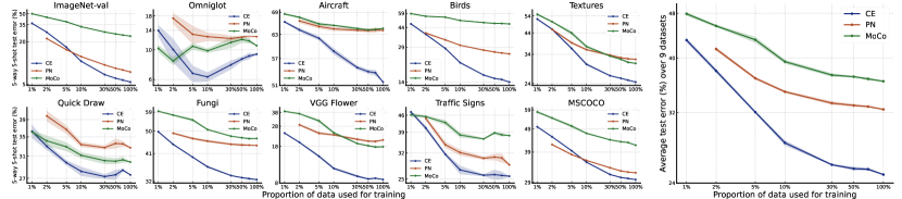
Figure 1: The effect of sample size per training class on few-shot classification performance. We use all $1000$ classes of the training set of ImageNet for training. Both axes are logit-scaled. ImageNet-val means conducting few-shot classification on the original validation set of ImageNet. The average performance is obtained by averaging performance on 9 datasets excluding ImageNet-val. Best viewed in color.

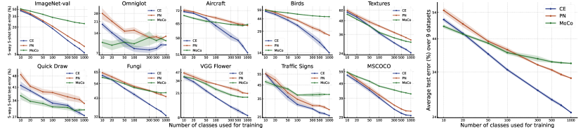
Figure 2: The effect of the number of training classes on few-shot classification performance. For each randomly selected class in ImageNet, we use all of its samples from the training set for training. Both axes are logit-scaled. Best viewed in color.

Neural scaling laws for training. Comparing Figure 1 and 2, we can see that for supervised models (CE and PN), increasing the number of classes is much more effective than increasing the number of samples per class (We give clearer comparisons in Figure 10-12 in the Appendix). The effect of increasing the number of samples per class plateaus quickly, while increasing the number of classes leads to very stable performance improvement throughout all scales. We notice that most performance curves of PN and CE in Figure 2 look like a straight line. In Figure 13-15 in the appendix we plot the linear fit which verifies our observations. In fact, the Pearson coefficient between the log scale of the number of training classes and the log scale of average test error is $-0.999$ for CE and $-0.995$ for PN, showing strong evidence of linearity. This linearity indicates the existence of a form of neural scaling laws in few-shot classification: test error falls off as a power law with the number of training classes, which is different from neural scaling laws observed in other machine learning tasks (Hestness et al., 2017; Zhai et al., 2022; Kaplan et al., 2020) that test error falls off as a power law with the number of training samples per class. Such a difference reveals the intrinsic difference between few-shot classification and other tasks: while seeing more samples in a training class does help in identifying new samples in the same class, it may not help that much in identifying previously-unseen classes in a new task. On the other hand, seeing more classes may help the model learn more potentially useful knowledge that might help distinguish new classes.

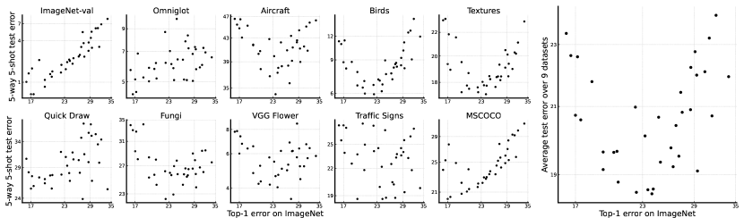
Figure 3: For supervised models, ImageNet performance is not a good predictor of few-shot classification performance. Each point in a plot refers to a supervised CE model with a specific backbone architecture. Both axes are logit-scaled.

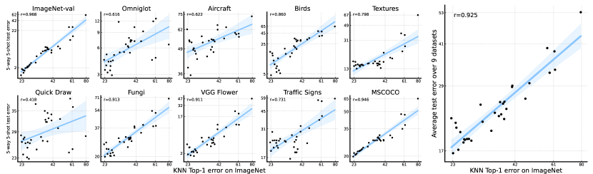
Figure 4: For self-supervised models, ImageNet performance is a good predictor of few-shot classification performance. Each point in a plot refers to a self-supervised model with a specific training algorithm/architecture. Both axes are logit-scaled. The regression line and a 95% confidence interval are plotted in blue. “r” refers to the correlation coefficient between the two axes of data.

Bigger is not necessarily better. On most evaluated datasets, test error decreases with more training samples/classes. However, on Omniglot and ISIC (shown in Figure 8-9), the error first goes down and then goes up, especially for supervised models. On the contrary, previous works (Snell et al., 2017) have shown that a simple PN model, both training and evaluating on Omniglot (class separated), can easily obtain a near-zero error. This indicates that as the number of training samples/classes increases, there exists a progressively larger mismatch between the knowledge learned from ImageNet and the knowledge needed for distinguishing new classes in these two datasets. Thus training a large model on a big dataset that can solve every possible task well is not a realistic hope, unless the training dataset already contains all possible tasks. How to choose a part of the training dataset to train a model on, or how to select positive/useful knowledge from a learned model depending on only a small amount of data in the specified adaptation scenario is an important research direction in few-shot classification.

CE training scales better. As seen from both figures, PN and MoCo perform comparably to CE on small-scale training data, but as more training data comes in, the gap gradually widens. Considering that all algorithms have been fed with the same amount of data during training, we can infer that CE training indeed scales better than PN and MoCo. This trend seems to be more obvious for fine-grained datasets including Aircraft, Birds, Fungi, and VGG Flower. While this phenomenon needs further investigation, we speculate it is due to that CE simultaneously differentiates all classes during training which requires distinguishing all possible fine-grained classes. On the contrary, meta-learning algorithms like PN typically need to distinguish only a limited number of classes during each iteration, and self-supervised models like MoCo do not use labels, thus focusing more on global information in images (Zhao et al., 2021) and performing not well on fine-grained datasets. We leave it for future work to verify if this conjecture holds generally.

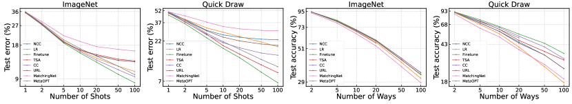
Figure 5: Way and shot experiments of adaptation algorithms on ImageNet and Quick Draw. For shot experiment, we fix the number of ways to 5 and show test error, and for way experiment, we fix the number of shots to 5 and show test accuracy. Both axes are logit-scaled. Best viewed in color.

4.2 ImageNet Performance vs Few-shot Performance

Then we fix the scale of training dataset and investigate how the changes in training algorithms and network architectures influence few-shot performance. We especially pay our attention to CE-trained and self-supervised models due to their superior performance shown in Table 1. Previous studies have revealed that the standard ImageNet performance of CE models trained on ImageNet is a strong predictor (with a linear relationship) of its performance on a range of vision tasks, including transfer learning (Kornblith et al., 2019), open-set recognition (Vaze et al., 2022) and domain generalization (Taori et al., 2020). We here ask if this observation also holds for few-shot classification. If this is true, we can improve few-shot classification on benchmarks that use ImageNet as the training dataset like Meta-Dataset, by just waiting for state-of-the-art ImageNet models. For this, we test 36 pre-trained supervised CE models with different network architectures, including VGG (Simonyan & Zisserman, 2015), ResNet (He et al., 2016), MobileNet (Howard et al., 2017), RegNet (Radosavovic et al., 2020), DenseNet (Huang et al., 2017), ViT (Dosovitskiy et al., 2021), Swin Transformer (Liu et al., 2021b) and ConvNext (Liu et al., 2022). We also test 32 self-supervised ImageNet pre-trained models with different network algorithms and architectures. The algorithms include MoCo-v2 (He et al., 2020), MoCo-v3 (Chen et al., 2021a), InstDisc (Wu et al., 2018), BYOL (Grill et al., 2020), SwAV (Caron et al., 2020), OBoW (Gidaris et al., 2021), SimSiam (Chen & He, 2021), Barlow Twins (Zbontar et al., 2021), DINO (Caron et al., 2021), MAE (He et al., 2022), iBOT (Zhou et al., 2022) and EsViT (Li et al., 2022a). We use KNN (Caron et al., 2021) to compute top-1 accuracy for these self-supervised models. We plot results for supervised models in Figure 3 and self-supervised models in Figure 4.

Supervised ImageNet models overfit to ImageNet performance. For supervised models, we can observe from Figure 3 that on most datasets sufficiently different from ImageNet, such as Aircraft, Birds, Textures, Fungi, and VGG Flower, the test error of few-shot classification first decreases and then increases with the improvement of ImageNet performance. The critical point is at about 23% Top-1 error on ImageNet, which is the best ImageNet performance in 2017 (e.g., DenseNet (Huang et al., 2017)). This indicates that recent years of improvement in image classification on ImageNet overfit to ImageNet performance when the downstream task is specified as few-shot classification. We also observe that on datasets like Quick Draw, Traffic Signs, and Ominglot, there is no clear relationship between ImageNet performance and few-shot performance. Since supervised ImageNet performance is usually a strong predictor of other challenging vision tasks, few-shot classification stands out to be a special task that needs a different and much better generalization ability. Identifying the reasons behind the difference may lead to a deeper understanding of both few-shot classification and vision representation learning.

ImageNet performance is a good predictor of few-shot performance for self-supervised models. Different from supervised models, for self-supervised models, we observe the clear positive correlation between ImageNet performance and few-shot classification performance. The best self-supervised model only obtains 77% top-1 accuracy on ImageNet, but obtains more than 83% average few-shot performance, outperforming all evaluated supervised models. Thus self-supervised algorithms indeed generalize better and the few-shot learning community should pay more attention to the progress of self-supervised learning.

5 Adaptation Analysis

In this section, we fix the training algorithm to the CE model trained on miniImageNet and analyze adaptation algorithms.

5.1 Way and Shot Analysis

Ways and shots are important variables during the adaptation phase of few-shot classification. For the first time, we analyze how the performance of different adaptation algorithms varies under different choices of ways and shots, with the training algorithm unchanged. For this experiment, we choose ImageNet and Quick Draw as the evaluated datasets because these two datasets have enough classes and images per class to be sampled and are representative for in-domain and out-of-domain datasets, respectively. For ImageNet, we remove all classes from miniImageNet.

Neural scaling laws for adaptation. We notice that for Logistic Regression, Finetune, and MetaOPT, the performance curves approximate straight lines when varying the number of shots. This indicates that for the scale of the adaptation dataset, the classification error obeys the traditional neural scaling laws (different from what we found for the scale of the training dataset in Section 4.1). While this seems to be a reasonable phenomenon for Finetune, we found it a surprise for Logistic Regression and MetaOpt, which are linear algorithms (for adaptation) built upon frozen features and are thus expected to reach performance saturation quickly. This reveals that even for small-scaled models trained on miniImageNet, the learned features are still quite linearly-separable for new tasks. However, their growth rates differ, indicating they differ in their capability to scale.

Table 2: The average support set size and the degree of task distribution shift of tasks from each dataset on three benchmarks. The metric measuring the degree of task distribution shift is defined by the deviation of feature importance; see Table 3 of Luo et al. (2022) for details.

Benchmark	miniImageNet	BSCD-FSL				Meta-Dataset
Dataset	miniImageNet	ChestX	ISIC	ESAT	CropD	ILSVRC	Omniglot	Aircraft	Birds	Textures	QuickD	Fungi	Flower	Traffic Sign	COCO
Mean support set size	5 or 25	25 or 100 or 250				374.5	88.5	337.6	316.0	287.3	425.2	361.9	292.5	421.2	416.1
Task distribution shift	0.056	0.186	0.205	0.153	0.101	0.054	0.116	0.097	0.117	0.100	0.106	0.080	0.096	0.150	0.083

Backbone adaptation is preferred for high-way, high-shot, or cross-domain tasks. As seen from Figure 5, while Finetune and the partial-finetune algorithm TSA do not significantly outperform other algorithms on 1-shot and 5-shot tasks on ImageNet, their advantages become greater when shots or ways increase or the task is conducted on Quick Draw. Thus we can infer that backbone adaptation is preferred when data scale is large enough to avoid overfitting or when the domain shift so large that the learned feature space deforms on the new domain.

Query-support matching algorithms scale poorly. Query-support matching algorithms like TSA, MatchingNet, NCC, and URL obtain query predictions by comparing the similarities of query features with support features, different from other algorithms that learn a classifier from the support set directly. As observed in Figure 5, all these algorithms perform well when the shot is 1 or 5, but scale weaker than power law as the number of shots increases except for TSA on Quick Draw where backbone adaptation is much preferred. Considering that URL as a flexible, optimizable linear head and TSA as a partial fine-tune algorithm have enough capacities for adaptation, their failure to scale well, especially on ImageNet, indicates that the objectives of query-support matching algorithms have fundamental optimization difficulties during adaptation when data scale increases.

5.2 Analysis of Finetune

As seen from Table 1 and Figure 5, vanilla Finetune algorithm performs always the best, even when evaluated on in-domain tasks with extremely scarce data. In particular, we have shown that recent partial-finetune algorithms, such as TSA and eTT that are designed to overcome this problem, both underperform vanilla Finetune algorithms. This is quite surprising since the initial Meta-Dataset benchmark (Triantafillou et al., 2020) shows that vanilla Finetune meets severe overfitting when data is extremely scarce.

The reasons lie in two aspects. First, in the original paper of Meta-Dataset, training and adaptation algorithms are bound together, so different adaptation algorithms use different backbones, making it unfair for comparison. This problem is then amplified later in the paper of TSA and eTT, where they use strong backbone for their own adaptation algorithms while copying the original results of Finetune in the benchmark. Second, previous works typically search for a single learning rate for Finetune. We found it important to separately search for the learning rates for backbone and the linear head. This simple change leads to a considerable performance improvement, as shown in Figure 6. We found that the optimal learning rate of backbone is typically much smaller than that of linear head.

We also wonder what is the critical factor that makes Finetune effective. In Figure 7, we show how the relative improvement of Finetune over PN changes when we increase total number of samples in the support set (way $\times$ shot). The relative improvement is quite close for all choices of ways, as long as the support set size does not change. Thus support set size is crucial for Finetune to be effective, which aligns with our intuition that the backbone can be adjusted more properly when seeing more data.

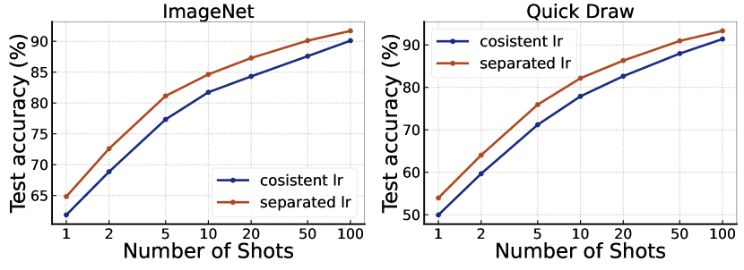
Figure 6: Comparisons of using consistent and separated learning rate for backbone and linear head during the finetune process.

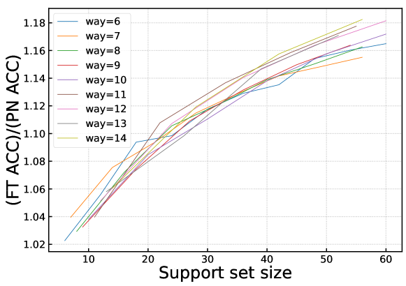
Figure 7: The advantages of Finetune increase as a function of the total number of samples in the support set.

Bias of evaluation protocols in different benchmarks. After analyzing the effectiveness of Finetune, we can now answer a question: why on traditional benchmarks like CIFAR, miniImageNet, tieredImageNet, the state-of-the-art algorithms do not adapt learned backbone during adaptation, but on benchmarks like BSCD-FSL and Meta-Dataset model adaptation becomes popular? As seen from Table 2, miniImageNet (similarly for CIFAR and tieredImageNet) has a small support set size of 5 or 25 and a small distribution shift from training to test datasets, while BSCD-FSL and Meta-Dataset have 10x larger support set size and encompass datasets with extremely large distribution shift. Thus according to our analysis, backbone adaptation algorithms such as Finetune do not have advantages on benchmarks like miniImageNet, especially when the learning rates are not separated; while on BSCD-FSL and Meta-Dataset, backbone needs adaptation towards new domains and abundant support samples make this possible. To avoid biased assessment, we recommend to the community that, besides reporting standard benchmark results, a method should also report the performance with different, specific ways and shots on datasets with different degrees of distribution shift.

6 Related Work

As an active research field, few-shot learning is considered to be a critical step towards building efficient and brain-like machines (Lake et al., 2017). Meta-learning (Thrun & Pratt, 1998; Schmidhuber, 1987; Naik & Mammone, 1992) was thought to be an ideal framework to approach this goal. Under this framework, methods can be roughly split into three branches: optimization-based methods, black-box methods, and metric-based methods. Optimization-based methods, mainly originated from MAML (Finn et al., 2017), learn the experience of how to optimize a neural network given a few training samples. Variants in this direction consider different parts of optimization to meta-learn, including model initialization point (Finn et al., 2017; Rusu et al., 2019; Rajeswaran et al., 2019; Zintgraf et al., 2019; Jamal & Qi, 2019; Lee et al., 2019), optimization process (Ravi & Larochelle, 2017; Xu et al., 2020; Munkhdalai & Yu, 2017; Li et al., 2017) or both (Baik et al., 2020; Park & Oliva, 2019). Black-box methods (Santoro et al., 2016; Garnelo et al., 2018; Mishra et al., 2018; Requeima et al., 2019) directly model the learning process as a neural network without explicit inductive bias. Metric-based methods (Vinyals et al., 2016; Snell et al., 2017; Sung et al., 2018; Yoon et al., 2019; Zhang et al., 2020) meta-learn a feature extractor that can produce a well-shaped feature space equipped with a pre-defined metric. In the context of few-shot image classification, most state-of-the-art meta-learning methods fall into the metric-based and optimization-based ones.

Recently, a number of non-meta-learning methods that utilize supervised (Chen et al., 2019; Tian et al., 2020; Dhillon et al., 2020; Triantafillou et al., 2021; Li et al., 2021) or unsupervised representation learning methods (Rizve et al., 2021; Doersch et al., 2020; Das et al., 2022; Hu et al., 2022; Xu et al., 2022a) to train a feature extractor have emerged to tackle few-shot image classification. In addition, a bunch of meta-learning methods (Chen et al., 2021b; Zhang et al., 2020; Hu et al., 2022; Ye et al., 2020) learn a model initialized from a pre-trained backbone (Our experiments also consider pretrain+meta-learning training algorithms such as Meta-Baseline, DeepEMD and FEAT. Thus our conclusions hold generally). Since these methods do not strictly follow meta-learning framework, the training algorithm does not necessarily have a relationship with the adaptation algorithm, and they are found to be simpler and more efficient than meta-learning methods while achieving better performance. Following this line, our paper further reveals that the training and adaptation phases in few-shot image classification are completely disentangled.

One relevant work (Sbai et al., 2020) also gives a detailed and comprehensive analysis of few-shot learning, especially on the training process. Our study complements this work in several ways: (1) the neural scaling laws that we found have not been discovered before, which proves the importance of the number of classes in few-shot learning. Although in Sbai et al. (2020) the significance of the number of classes has also been discussed from different perspectives, there are no clear conclusions in Sbai et al. (2020) and thus we complement their studies; (2) we observed that larger datasets may lead to degraded performance in specific downstream datasets, both in terms of increasing the number of classes and samples per class. Such findings were not present in Sbai et al. (2020), and hence our study opens new avenues for future research by inspecting specific datasets; (3) there’s no clear evidence in Sbai et al. (2020) that simple supervised training scales better than other types of training algorithms; (4) moreover, our paper evaluates 18 datasets, including those beyond ImageNet and CUB, which are the only ones studied in Sbai et al. (2020). Thus, our study provides a broader perspective and complements the analysis in Sbai et al. (2020).

7 Discussion

One lesson learned from our analysis is that training by only scaling models and datasets is not a one-fit-all solution. Either the design of the training objective should consider what the adaptation dataset is (instead of the adaptation algorithm), or the adaptation algorithm should select accurate training knowledge of interest. The former approach limits the trained model to a specific target domain, while the latter approach cannot be realized easily when only few labeled data are provided in the target task which makes knowledge selection difficult or even impossible due to bias of distribution estimation (Luo et al., 2022; Xu et al., 2022b). More effort should be put into aligning training knowledge and knowledge needed in adaptation. Although we have shown vanilla Finetune performs so well, we believe that such a brute-force, non-selective model adaptation algorithm is not the final solution, and it has other drawbacks such as having extremely high adaptation cost, as shown in Appendix D. Viewed from another perspective, our work points to the plausibility of using few-shot classification as a tool to better understand some key aspects of general visual representation learning.

Appendix A Additional Related Work

Few-shot classification benchmarks. Earlier benchmarks in few-shot image classification focus on in-domain classification with standard 5-way 1-shot and 5-shot settings, including miniImageNet (Vinyals et al., 2016), FC100 (Oreshkin et al., 2018) and tieredImageNet (Ren et al., 2018). BSCD-FSL benchmark (Guo et al., 2020) targets at a more realistic cross-domain setting and considers the evaluation of higher shots such as 20 or 50. Meta-Dataset (Triantafillou et al., 2020) also targets cross-domain settings, but goes further and considers imbalanced classes and varying numbers of ways and shots. MD+VTAB (Dumoulin et al., 2021) further combines Meta-Dataset and VTAB (Zhai et al., 2019) from transfer learning, aiming at connecting few-shot classification with general visual representation learning. Although all benchmarks evaluate the models’ ability to quickly adapt to new few-shot classification tasks, state-of-the-art methods from different benchmarks differ a lot. In this paper, through a fine-grained test-time analysis, we figure out the reason behind this phenomenon.

Backbone adaptation in few-shot classification. MAML (Finn et al., 2017) is the first paper that uses Finetune as the adaptation algorithm. However, all hyperparameters of Finetune are fixed before training and the backbone is weak, so MAML does not perform well. Later, Tadam (Oreshkin et al., 2018) designs the first adaptation algorithm that partially adapts the backbone by a black-box meta-learning method. The Baseline algorithm (Chen et al., 2019) is the first one that uses a combination of non-meta-learning training and Finetune, and achieves surprisingly good results. Another baseline method (Dhillon et al., 2020) utilizes simple supervised training and Finetune using initialization of the linear layer from feature prototypes. CNAPs (Requeima et al., 2019) is a partial adaptation meta-learning algorithm that learns on multiple datasets on Meta-Dataset and achieves SOTA results. After CNAPs comes out, several works emerge that adapt the backbone either by finetuning or partial backbone adaptation in the adaptation phase on Meta-Dataset (Triantafillou et al., 2021; Li et al., 2022b; Xu et al., 2022a; Patacchiola et al., 2022; Liu et al., 2021a; Bateni et al., 2020; Shysheya et al., 2023). Our paper reveals that the popularity of this line of research first declined and then increased is related to the bias of evaluation protocols of benchmarks.

Connections of pre-trained models with downstream task performance. Kornblith et al. (2019) showed that ImageNet performance has a linear relationship with the downstream transfer performance of classification tasks. Similarly, such a linear relationship was discovered later in domain generalization (Taori et al., 2020) and open-set recognition (Vaze et al., 2022). Abnar et al. (2022) questioned this result with large-scale experiments and showed that when increasing the upstream accuracy to a very high number, performance of downstream tasks can saturate. Our experiments on Omniglot and ISIC further ensure this observation, even when the training data is at a small scale. Recently, Entezari et al. (2023) find that the choice of the pre-training data source is essential for the few-shot classification, but its role decreases as more data is made available for fine-tuning, which complements our study.

Appendix B Details of Experiments

We reimplement some of the training algorithms in Table 1, including all PN models, all MAML models, CE models with Conv-4 and ResNet-12, MetaOpt, Meta-Baseline, COS, and IER. For all other training algorithms, we use existing checkpoints from official repositories or the Pytorch library (Paszke et al., 2019). All reimplemented models are trained for 60 epochs using SGD+Momemtum with cosine learning rate decay without restart. The initial learning rates are all set to 0.1. Training batchsize is 4 for meta-learning models and 256 for non-meta-learning models. The input image size is 84$\times$84 for Conv-4 and ResNet-12 models and 224$\times$224 for other models. We use random crop and horizontal flip as data augmentation at training. Since some models like PN are trained on normalized features, for a fair comparison, we normalize the features of all models for the adaptation phase.

For experiments in Section 4.1, to make a fair comparison, we train CE and MoCo for 150 epochs and train PN using a number of iterations that makes the number of seen samples equal. SGD+Momemtum with cosine learning rate decay without restart is used. The backbone used is ResNet-18. Learning rates are all set to 0.1. Training batchsize is 4 for PN and 256 for CE and MoCo. The input image size is 84$\times$84. During training, we use random crop and horizontal flip as data augmentation for CE and PN, and for MoCo, we use the same set of data augmentations as in the MoCo-v2 paper (Chen et al., 2020). We repeat training 5 times with different sampling of data or classes for each experiment in Section 4.1. All pre-trained supervised models in Section 4.2 are from Pytorch library, and all self-supervised models are from official repositories. To avoid memory issues, we only use 500000 image features of the training set of ImageNet for KNN computation of Top-1 ImageNet accuracy for self-supervised models in Section 4.2.

All training algorithms that are evaluated in this paper, including meta-learning algorithms, set the learnable parameters as the parameters of a feature extractor, and all adaptation algorithms do not have additional parameters that need to be obtained from training. Thus adapting different training algorithms is as easy as adapting different feature extractors with different adaptation algorithms. There exist other meta-learning algorithms (Oreshkin et al., 2018; Requeima et al., 2019; Patacchiola et al., 2022; Ye et al., 2020; Doersch et al., 2020) that meta-learn additional parameters besides a feature extractor, so their training/adaptation algorithms cannot be combined with other adaptation/training algorithms directly. Thus these algorithms are not included in our experiments. One solution is, for each such algorithm, learn the same additional parameters while freezing the backbone for every other trained model, and then we can compare all algorithms. We expect that after doing this the ranking of both training and adaptation algorithms will still not be changed and we leave it for future work to verify this conjecture.

Throughout the main paper, for all adaptation algorithms that have hyperparameters, we grid search hyperparameters on the validation dataset of miniImageNet and Meta-Dataset. For Traffic Signs which does not have a validation set, we use the hypeparameters averaged over the found optimal hyperparameters of all other datasets. For adaptation analysis experiments in Section 5, we partition ImageNet and Quick Draw to have a 100-class validation set. The rest is used as the test set.

Appendix C Additional Tables, Figures, and Analysis

C.1 Additional Tables for Section 3.2

Table 3 shows 5-way 1-shot results similar to Table 1. Table 4 and Table 5 show similar results on miniImageNet. All results lead to the same conclusion that training and adaptation algorithms are uncorrelated. One thing to notice in Table 3 is that CE model using ViT-base as backbone trained on ImageNet performs particularly well in 1-shot setting. It outperforms DINO in 1-shot setting while underperforms DINO in 5-shot setting. Also, MAML model on Meta-Dataset performs much better than the same model on miniImageNet (possibly due to the use of transductive BN which gives additional unfair flexibility towards new domains). These phenomena show that although training and adaptation algorithms are uncorrelated, the ranking of training algorithms can be influenced by the change of evaluated tasks. Further understanding of how these factors influence the performance of training models is needed in the future.

Table 3: 5-way 1-shot performance of pairwise combinations of a variety of training and adaptation algorithms on Meta-Dataset. We exclude MatchingNet from the adaptation algorithms because MatchingNet equals NCC when the shot is one.

			Adaptation algorithm
Training algorithm	Training dataset	Architecture	MetaOpt	NCC	LR	URL	CC	TSA/eTT	Finetune
PN	miniImageNet	Conv-4	38.50$\pm$0.5	38.69$\pm$0.5	38.23$\pm$0.4	38.81$\pm$0.4	38.64$\pm$0.5	41.27$\pm$0.5	42.60$\pm$0.5
MAML	miniImageNet	Conv-4	42.92$\pm$0.5	43.00$\pm$0.5	42.65$\pm$0.5	42.51$\pm$0.5	42.97$\pm$0.5	44.55$\pm$0.5	46.13$\pm$0.5
CE	miniImageNet	Conv-4	44.49$\pm$0.5	44.88$\pm$0.5	44.88$\pm$0.5	44.48$\pm$0.5	44.82$\pm$0.5	46.20$\pm$0.5	46.92$\pm$0.5
MatchingNet	miniImageNet	ResNet-12	45.00$\pm$0.5	45.23$\pm$0.5	45.24$\pm$0.5	44.89$\pm$0.5	45.40$\pm$0.5	46.18$\pm$0.5	48.53$\pm$0.5
MAML	miniImageNet	ResNet-12	46.09$\pm$0.5	46.09$\pm$0.5	45.81$\pm$0.5	45.88$\pm$0.5	46.07$\pm$0.5	51.95$\pm$0.5	53.71$\pm$0.5
PN	miniImageNet	ResNet-12	47.32$\pm$0.5	47.53$\pm$0.5	47.33$\pm$0.5	47.53$\pm$0.5	47.65$\pm$0.5	49.36$\pm$0.5	53.06$\pm$0.5
MetaOpt	miniImageNet	ResNet-12	49.16$\pm$0.5	49.52$\pm$0.5	49.53$\pm$0.5	49.42$\pm$0.5	49.73$\pm$0.5	52.01$\pm$0.5	53.90$\pm$0.5
CE	miniImageNet	ResNet-12	51.09$\pm$0.5	51.42$\pm$0.5	51.60$\pm$0.5	50.94$\pm$0.5	51.71$\pm$0.5	53.81$\pm$0.5	54.68$\pm$0.5
Meta-Baseline	miniImageNet	ResNet-12	51.24$\pm$0.5	51.56$\pm$0.5	51.67$\pm$0.5	51.23$\pm$0.5	51.77$\pm$0.5	53.87$\pm$0.5	54.54$\pm$0.5
COS	miniImageNet	ResNet-12	51.23$\pm$0.5	51.53$\pm$0.5	51.31$\pm$0.5	51.87$\pm$0.5	51.72$\pm$0.5	54.18$\pm$0.5	54.98$\pm$0.5
PN	ImageNet	ResNet-50	52.50$\pm$0.5	52.84$\pm$0.5	52.71$\pm$0.5	52.90$\pm$0.5	52.93$\pm$0.5	54.34$\pm$0.5	57.40$\pm$0.5
IER	miniImageNet	ResNet-12	53.31$\pm$0.5	53.63$\pm$0.5	53.82$\pm$0.5	53.24$\pm$0.5	53.98$\pm$0.5	56.32$\pm$0.5	56.98$\pm$0.5
Moco v2	ImageNet	ResNet-50	54.89$\pm$0.5	55.38$\pm$0.5	55.64$\pm$0.5	55.77$\pm$0.5	55.70$\pm$0.5	58.13$\pm$0.5	59.99$\pm$0.5
DINO	ImageNet	ResNet-50	60.81$\pm$0.5	61.37$\pm$0.5	61.61$\pm$0.5	61.96$\pm$0.5	61.81$\pm$0.5	62.69$\pm$0.5	63.61$\pm$0.5
CE	ImageNet	ResNet-50	62.34$\pm$0.5	62.88$\pm$0.5	62.90$\pm$0.5	63.55$\pm$0.5	63.18$\pm$0.5	65.04$\pm$0.5	65.87$\pm$0.5
BiT-S	ImageNet	ResNet-50	62.41$\pm$0.5	62.95$\pm$0.5	63.15$\pm$0.5	63.40$\pm$0.5	63.40$\pm$0.5	65.02$\pm$0.5	67.05$\pm$0.5
CE	ImageNet	Swin-B	64.03$\pm$0.5	64.46$\pm$0.5	64.38$\pm$0.5	65.22$\pm$0.5	65.01$\pm$0.5	-	69.12$\pm$0.5
DeiT	ImageNet	ViT-B	64.20$\pm$0.5	64.62$\pm$0.5	64.43$\pm$0.5	65.31$\pm$0.5	65.11$\pm$0.5	66.25$\pm$0.5	69.12$\pm$0.5
DINO	ImageNet	ViT-B	64.86$\pm$0.5	65.36$\pm$0.5	65.31$\pm$0.5	66.05$\pm$0.5	65.91$\pm$0.5	67.26$\pm$0.5	67.89$\pm$0.5
CE	ImageNet	ViT-B	67.19$\pm$0.5	67.61$\pm$0.5	67.56$\pm$0.5	68.00$\pm$0.5	67.85$\pm$0.5	69.78$\pm$0.5	72.14$\pm$0.4
CLIP	WebImageText	ViT-B	67.95$\pm$0.5	68.68$\pm$0.5	69.10$\pm$0.5	69.85$\pm$0.5	68.85$\pm$0.5	70.42$\pm$0.5	74.96$\pm$0.5

Table 4: 5-way 5-shot performance of pairwise combinations of a variety of training and adaptation algorithms conducted on the miniImageNet benchmark.

		Adaptation algorithm
Training algorithm	Architecture	MatchingNet	MetaOpt	NCC	LR	URL	CC	TSA/eTT	Finetune
MAML	Conv-4	59.80$\pm$0.3	57.99$\pm$0.4	58.86$\pm$0.2	60.93$\pm$0.3	60.81$\pm$0.4	61.83$\pm$0.3	62.40$\pm$0.3	62.03$\pm$0.5
PN	Conv-4	63.71$\pm$0.5	64.12$\pm$0.5	63.67$\pm$0.5	65.78$\pm$0.5	65.78$\pm$0.4	65.82$\pm$0.5	65.69$\pm$0.4	66.35$\pm$0.5
CE	Conv-4	64.09$\pm$0.4	66.41$\pm$0.4	67.93$\pm$0.3	68.92$\pm$0.5	68.63$\pm$0.4	69.08$\pm$0.5	69.22$\pm$0.4	69.51$\pm$0.6
MatchingNet	ResNet-12	69.48$\pm$0.3	69.71$\pm$0.3	69.75$\pm$0.6	70.92$\pm$0.4	70.86$\pm$0.4	71.00$\pm$0.4	71.15$\pm$0.2	72.31$\pm$0.4
MAML	ResNet-12	70.27$\pm$0.3	68.37$\pm$0.6	70.09$\pm$0.4	71.94$\pm$0.4	71.33$\pm$0.3	72.10$\pm$0.5	75.70$\pm$0.5	76.18$\pm$0.3
PN	ResNet-12	73.64$\pm$0.4	74.03$\pm$0.4	74.99$\pm$0.5	75.46$\pm$0.4	75.72$\pm$0.4	75.65$\pm$0.4	76.99$\pm$0.3	79.62$\pm$0.2
MetaOpt	ResNet-12	75.21$\pm$0.4	76.51$\pm$0.5	77.69$\pm$0.4	78.09$\pm$0.5	78.36$\pm$0.4	78.43$\pm$0.4	80.55$\pm$0.2	81.44$\pm$0.2
CE	ResNet-12	76.66$\pm$0.4	77.66$\pm$0.4	79.97$\pm$0.4	80.01$\pm$0.5	80.11$\pm$0.5	80.34$\pm$0.5	80.65$\pm$0.1	80.84$\pm$0.2
Meta-Baseline	ResNet-12	77.06$\pm$0.4	77.59$\pm$0.4	79.85$\pm$0.2	80.54$\pm$0.5	80.52$\pm$0.4	80.77$\pm$0.4	80.97$\pm$0.3	81.42$\pm$0.2
COS	ResNet-12	79.70$\pm$0.3	80.07$\pm$0.4	81.01$\pm$0.3	81.28$\pm$0.4	81.54$\pm$0.4	81.52$\pm$0.5	81.97$\pm$0.2	83.26$\pm$0.2
IER	ResNet-12	80.37$\pm$0.3	81.33$\pm$0.3	82.80$\pm$0.3	83.71$\pm$0.3	83.83$\pm$0.3	84.04$\pm$0.3	83.53$\pm$0.3	84.02$\pm$0.2

Table 5: 5-way 1-shot performance of pairwise combinations of a variety of training and adaptation algorithms conducted on the miniImageNet benchmark.

		Adaptation algorithm
Training algorithm	Architecture	MetaOpt	NCC	LR	URL	CC	TSA/eTT	Finetune
MAML	Conv-4	45.97$\pm$0.4	46.24$\pm$0.5	47.62$\pm$0.5	46.81$\pm$0.6	47.40$\pm$0.5	47.55$\pm$0.4	47.40$\pm$0.3
PN	Conv-4	49.79$\pm$0.4	50.95$\pm$0.4	50.89$\pm$0.4	51.01$\pm$0.5	50.95$\pm$0.4	50.97$\pm$0.3	50.65$\pm$0.4
CE	Conv-4	51.28$\pm$0.5	51.68$\pm$0.7	51.07$\pm$0.6	52.18$\pm$0.6	51.86$\pm$0.7	52.88$\pm$0.3	51.87$\pm$0.4
MatchingNet	ResNet-12	54.52$\pm$0.5	54.96$\pm$0.5	54.85$\pm$0.5	54.84$\pm$0.6	54.89$\pm$0.5	55.27$\pm$0.4	55.52$\pm$0.4
MAML	ResNet-12	56.43$\pm$0.4	55.80$\pm$0.7	57.14$\pm$0.7	56.06$\pm$0.8	57.03$\pm$0.7	57.86$\pm$0.4	58.49$\pm$0.2
PN	ResNet-12	59.91$\pm$0.4	60.25$\pm$0.7	60.26$\pm$0.7	60.01$\pm$0.6	60.26$\pm$0.7	60.37$\pm$0.5	60.67$\pm$0.2
MetaOpt	ResNet-12	60.40$\pm$0.3	60.82$\pm$0.5	60.40$\pm$0.5	61.79$\pm$0.5	60.91$\pm$0.5	61.89$\pm$0.4	62.58$\pm$0.4
CE	ResNet-12	62.53$\pm$0.6	62.88$\pm$0.6	62.55$\pm$0.6	63.15$\pm$0.6	62.94$\pm$0.6	63.46$\pm$0.4	63.33$\pm$0.4
Meta-Baseline	ResNet-12	63.99$\pm$0.2	64.92$\pm$0.7	64.84$\pm$0.7	64.55$\pm$0.7	64.91$\pm$0.7	64.92$\pm$0.3	64.97$\pm$0.2
COS	ResNet-12	64.06$\pm$0.3	64.73$\pm$0.9	64.71$\pm$0.9	64.60$\pm$0.8	64.70$\pm$0.9	64.92$\pm$0.4	65.01$\pm$0.4
IER	ResNet-12	65.05$\pm$0.1	66.45$\pm$0.6	66.17$\pm$0.6	66.68$\pm$0.6	66.48$\pm$0.6	66.25$\pm$0.3	65.86$\pm$0.4

C.2 Additional Figures and Analysis for Section 4.1

Figure 8 and Figure 9 show the data-scaling experiments evaluated on other 9 datasets from BSCD-FSL Benchmark and DomainNet. The general trend is similar to the trend on Meta-Dataset. ISIC shows similar phenomenon to Omniglot in that few-shot performance may not improve if we use larger datasets. But one difference is that for MoCo, few-shot performance does always improve on ISIC, while few-shot performance does not always improve on Omniglot. Also, MoCo performs well on ChestX, while falling behind CE and PN on all other datasets. These show that the knowledge learned from MoCo is somewhat different from that of PN and CE, and this knowledge is useful for classification tasks on ISIC and ChestX. Previous works (Zhao et al., 2021) has shown that contrastive learning models like MoCo tend to learn more low-level visual features that are easier to transfer. We thus conjecture that low-level knowledge is more important for tasks of some datasets such as ChestX and ISIC. This indicates that the design of the training objective should consider what the test dataset is, so a one-fit-all solution may not exist. We also notice that all datasets in DomainNet except for Quick Draw exhibit similar scale patterns. We know that in DomainNet, each dataset has the same set of classes, while differs in domains. Thus we can infer that the test domain is not the key factor that influences the required training knowledge, but the choice of classes is. In (Luo et al., 2022), the authors define a new task distribution shift that measures the difference between tasks, taking classes into consideration. It is future work to see whether task distribution shift is the key factor that influences the required training knowledge for each test dataset.

Figure 10-12 depicts the comparisons of the two data scaling approaches for CE, PN, and MoCo. We can see that for CE and PN, increasing the number of classes is far more effective than increasing the number of samples per class. However, for MoCo, two data scaling approaches present similar performance at every data ratio used for training. Thus we can infer that self-supervised algorithms that do not use labels for supervision indeed do not be influenced by the number of labels. Self-supervised algorithms do not rely on labels, so they treat each sample equally, especially for contrastive learning methods. Thus for self-supervised algorithms, the total number of training samples is the only variable of interest. While this makes self-supervised algorithms particularly suitable for learning on datasets with scarce classes, this also hinders self-supervised algorithms from scaling well to datasets with a large number of classes, e.g., ImageNet-21K or JFM (Sun et al., 2017).

Figure 13-15 plot the linear fit of few-shot performance vs the number of training classes on logit-transformed axes. We can see that the linear relationship is obvious for most circumstances (most correlation coefficients are larger than 0.9). Thus we have verified the discovery of neural scaling laws wrt the number of training classes.

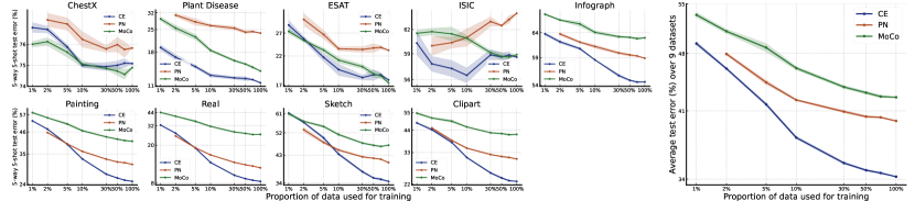
Figure 8: Results of other 9 datasets from BSCD-FSL benchmark and DomainNet about the effect of sample size per training class on few-shot classification performance. The plot follows Figure 1.

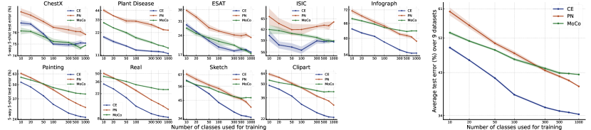
Figure 9: Results of other 9 datasets from BSCD-FSL benchmark and DomainNet about the effect of the number of training classes on few-shot classification performance. The plot follows Figure 2.

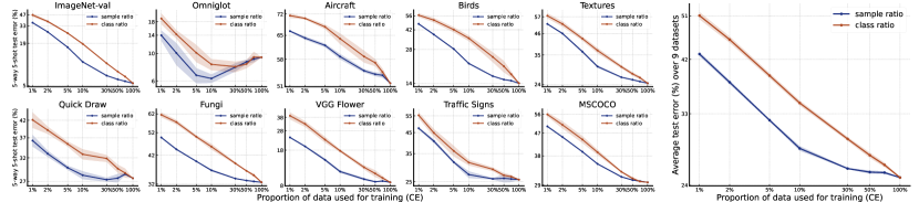
Figure 10: Comparisons of the two data scaling approaches for CE: scaling with sample size per training class and scaling with the number of training classes.

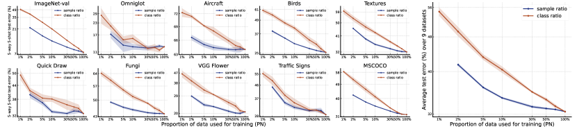
Figure 11: Comparisons of the two data scaling approaches for PN.

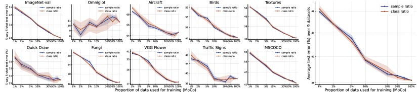
Figure 12: Comparisons of the two data scaling approaches for MoCo.

Figure 13: Linear fit of few-shot performance of CE vs the number of training classes on logit-transformed axes. “r” refers to the correlation coefficient between two axes of data.

Figure 14: Linear fit of few-shot performance of PN vs the number of training classes on logit-transformed axes. “r” refers to the correlation coefficient between two axes of data.

Figure 15: Linear fit of few-shot performance of MoCo vs the number of training classes on logit-transformed axes. “r” refers to the correlation coefficient between two axes of data.

Table 6: Detailed results of supervised CE models in Figure 3. Bold/underline is the best/second best in each column.

Architecture	ImageNet Top-1	Avg few-shot	ImageNet-val	Omniglot	Aircraft	Birds	Textures	Quick Draw	Fungi	VGG Flower	Traffic Signs	MSCOCO
ResNet-18	68.55	79.29	96.76	92.73	59.19	90.95	79.81	70.16	73.97	94.31	78.22	74.24
ResNet-34	72.50	79.18	97.66	92.76	58.65	91.71	81.57	68.57	73.54	93.80	76.27	75.77
ResNet-50	75.27	79.33	98.15	92.93	59.51	92.02	82.26	67.67	72.68	94.33	75.17	77.41
ResNet-101	76.74	79.89	98.46	92.98	60.10	92.90	81.97	69.10	74.09	94.54	75.50	77.84
ResNet-152	77.73	79.02	98.62	91.33	57.20	93.36	82.36	68.12	73.85	94.26	72.37	78.37
Swin-T	80.74	80.86	99.14	94.17	58.26	93.40	82.70	73.70	74.77	95.23	76.30	79.20
Swin-S	82.59	79.41	99.33	93.17	56.94	91.89	81.07	74.14	72.01	93.25	72.68	79.58
Swin-B	83.00	79.27	99.33	94.87	55.26	91.25	80.63	74.54	70.71	93.99	72.32	79.82
ViT-B	80.74	80.36	98.92	94.98	58.16	92.23	80.48	73.02	71.71	93.45	81.33	77.83
ViT-L	79.50	80.34	98.80	93.85	59.26	93.04	81.32	74.53	72.07	94.80	78.21	76.02
DenseNet-121	73.60	80.78	97.52	94.88	61.62	92.89	81.62	71.95	74.30	94.73	79.58	75.49
DenseNet-161	76.44	81.42	98.05	93.92	65.87	93.00	82.21	70.71	74.42	95.40	80.09	77.12
DenseNet-169	75.07	80.65	97.78	93.60	61.71	92.43	81.77	69.55	74.28	94.98	81.21	76.29
DenseNet-201	75.86	81.40	97.97	94.91	61.97	93.32	82.24	73.31	73.08	95.33	81.33	77.09
RegNetY-1.6GF	76.01	81.53	97.88	94.19	62.72	93.85	82.84	72.00	77.08	95.97	77.82	77.31
RegNetY-3.2GF	77.63	81.49	98.22	93.84	63.25	94.07	82.70	72.26	77.66	95.84	75.89	77.93
RegNetY-16GF	79.39	81.21	98.57	94.82	62.16	94.02	82.46	72.34	75.79	95.68	75.03	78.62
RegNetY-32GF	79.79	80.37	98.69	94.24	59.72	93.57	82.23	72.41	74.37	95.80	72.06	78.94
RegNetX-400MF	71.45	79.10	97.16	93.20	57.76	91.57	80.91	70.06	73.46	94.25	75.50	75.14
RegNetX-800MF	73.86	80.24	97.65	93.62	59.13	92.36	82.33	69.69	75.78	95.07	77.49	76.70
MobileNetV2	70.54	80.90	96.86	94.26	61.03	91.87	80.61	73.30	76.13	95.56	80.64	74.70
MobileNetV3-L	72.91	80.48	94.71	94.91	56.63	91.45	80.68	76.11	74.65	96.49	81.22	72.21
MobileNetV3-S	66.10	78.06	91.78	93.45	53.79	88.05	77.03	74.64	72.50	94.16	80.21	68.72
VGG-11	67.97	75.99	93.13	93.08	54.21	85.19	78.89	65.61	70.57	93.59	72.81	69.95
VGG-11-BN	69.54	77.90	93.99	94.14	58.48	87.45	81.01	64.46	73.28	94.83	76.76	70.66
VGG-13	68.93	76.78	93.96	93.98	54.94	87.16	79.71	66.61	70.64	93.29	73.91	70.78
VGG-13-BN	70.64	78.01	94.64	92.84	58.83	88.87	81.56	64.81	74.26	94.83	74.43	71.64
VGG-16	70.86	77.24	95.63	92.66	55.63	89.91	79.88	62.25	72.16	93.62	76.00	73.02
VGG-16-BN	72.68	78.56	96.33	91.65	60.85	91.32	81.84	62.08	74.45	93.82	76.70	74.33
VGG-19	71.41	77.76	96.25	94.96	57.42	90.78	79.52	64.16	71.08	91.43	76.43	74.03
VGG-19-BN	73.26	79.58	96.77	92.18	64.29	91.80	81.57	65.23	73.43	93.15	79.82	74.80
ConvNeXt-T	81.69	78.22	97.91	94.76	54.78	91.22	78.45	72.74	65.88	93.62	77.44	75.12
ConvNeXt-S	82.84	77.41	98.42	95.54	53.58	88.60	78.18	72.53	67.26	92.63	76.10	72.29
ConvNeXt-B	83.35	77.37	98.66	95.65	54.58	89.09	76.79	71.86	66.99	92.16	74.45	74.73
ConvNeXt-L	83.69	76.62	98.99	94.31	53.50	88.72	76.92	69.44	66.04	92.22	72.32	76.10

Table 7: Detailed results of self-supervised models in Figure 4. Bold/underline is the best/second best in each column.

Algorithm	Architecture	ImageNet Top-1	Avg few-shot	ImageNet-val	Omniglot	Aircraft	Birds	Textures	Quick Draw	Fungi	VGG Flower	Traffic Signs	MSCOCO
BYOL	ResNet-50	62.20	77.91	92.72	92.96	52.99	80.78	83.81	73.34	70.77	96.25	81.04	69.30
SwAV	ResNet-50	62.10	74.53	93.37	92.66	45.37	71.12	85.20	65.71	69.84	95.18	73.72	71.98
SwAV	ResNet-50-x2	62.59	74.93	92.57	94.71	45.41	68.11	85.17	68.34	70.16	95.70	75.40	71.37
SwAV	ResNet-50-x4	63.65	74.60	92.40	93.89	44.99	66.26	85.71	67.71	70.16	95.53	76.38	70.80
SwAV	ResNet-50-x5	61.37	75.99	93.38	92.71	46.41	69.65	86.77	67.27	72.16	96.60	79.72	72.62
DINO	ViT-S/8	76.94	83.33	98.16	96.61	61.20	95.33	85.93	73.48	80.06	98.10	80.50	78.71
DINO	ViT-S/16	72.48	81.52	97.28	95.01	56.88	94.80	85.63	73.00	79.51	97.88	74.81	76.19
DINO	ViT-B/16	74.15	81.39	97.91	95.77	50.72	92.39	86.15	73.58	79.77	98.28	78.25	77.63
DINO	ViT-B/8	75.74	82.85	98.34	96.83	64.67	89.71	87.02	72.39	78.83	98.21	79.03	78.96
DINO	ResNet-50	64.09	77.37	93.98	93.72	51.60	77.48	84.78	65.07	75.51	96.98	78.84	72.37
MoCo-v1	ResNet-50	41.27	67.67	87.98	88.05	41.44	61.77	77.96	61.06	61.69	89.39	62.64	65.01
MoCo-v2-200epoch	ResNet-50	51.72	70.33	93.10	90.79	36.12	65.43	82.28	67.49	60.52	91.00	68.52	70.81
MoCo-v2	ResNet-50	59.19	71.24	94.70	89.73	34.38	70.32	84.03	66.13	61.74	91.92	70.78	72.10
MoCo-v3	ResNet-50	66.61	79.95	94.91	94.61	55.45	87.31	84.75	72.27	72.75	96.68	83.44	72.32
MoCo-v3	ViT-S	65.46	76.75	94.22	93.41	45.94	84.66	83.77	73.21	69.56	94.99	72.81	72.39
MoCo-v3	ViT-B	69.32	78.40	95.80	94.66	47.08	85.29	84.74	75.19	72.53	96.04	76.33	73.70
SimSiam	ResNet-50	53.57	73.88	92.07	92.87	44.38	68.01	81.84	70.05	66.67	94.67	77.05	69.37
Barlow Twins	ResNet-50	63.26	77.04	93.83	92.23	49.89	79.07	84.73	68.31	71.23	96.35	81.04	70.53
MAE	ViT-B	20.66	46.77	39.94	93.45	26.89	35.54	33.04	72.07	30.66	52.6	41.64	35.01
MAE	ViT-L	42.63	60.38	72.40	95.61	40.42	49.91	61.76	75.85	46.74	77.07	43.40	52.70
MAE	ViT-H	38.50	61.43	72.32	95.36	40.96	50.97	63.64	75.11	48.91	80.02	44.64	53.27
IBOT	Swin-T/7	73.61	81.26	97.74	97.05	52.37	88.36	85.40	77.16	77.05	97.46	79.16	77.37
IBOT	Swin-T/14	74.50	81.79	97.97	96.65	51.67	93.21	85.62	76.86	79.64	97.75	76.90	77.83
IBOT	ViT-S	73.12	81.25	97.54	95.67	53.97	93.91	85.32	73.77	78.23	97.66	75.82	76.86
IBOT	ViT-B	75.28	80.16	98.04	95.8	47.01	91.57	85.21	73.78	76.57	97.81	75.63	78.02
IBOT	ViT-L	76.37	78.59	98.27	96.18	45.60	84.78	84.02	76.27	72.93	97.18	70.92	79.46
EsViT	ResNet-50	69.91	75.14	97.21	88.21	42.87	80.45	84.85	62.87	70.33	95.04	75.90	75.70
EsViT	Swin-T	74.32	81.31	97.84	96.25	50.78	94.44	85.75	74.80	78.57	97.83	75.64	77.72
EsViT	Swin-S	76.19	79.43	98.55	94.93	46.50	86.50	85.52	72.77	76.41	97.15	75.71	79.33
EsViT	Swin-B	77.33	77.77	98.77	95.59	37.74	83.57	83.76	71.88	73.98	96.62	76.64	80.19
oBoW	ResNet-50	59.09	70.93	93.79	92.85	37.98	68.85	78.86	67.91	62.93	89.45	67.09	72.49
InstDisc	ResNet-50	38.13	66.85	84.70	87.18	43.25	60.72	74.23	63.84	61.34	89.54	59.42	62.14

C.3 Detailed Results of Figures in Section 4.2

Table 6 and Table 7 show the detailed performance of supervised and self-supervised models in Section 4.2.

C.4 Additional Analysis for Section 5

In Figure 5, the few-shot performance is quite close on ImageNet than on Quick Draw. While LR, Finetune, and MetaOPT all follow the power law, their rates are different. All query-support matching algorithms perform similarly to NCC on ImageNet, showing their difficulties to utilize the capacities for generalizing to in-domain tasks. We notice that Cosine Classifier (CC) as a metric-based method performs much better than other metric-based methods when the number of shots is large on ImageNet. This verifies that it is query-support matching that makes algorithms scale poorly, not the use of metric space. We also notice that the behaviors of different algorithms are quite different. While Logistic Regression (LR) performs relatively well when the number of shots increases, its performance quickly drops when the number of ways increases. The ranking of other algorithms such as CC and MetaOPT changes with different situations. It is future work to figure out what influences the performance of these algorithms.

Appendix D Finetune has High Adaptation Cost

For adaptation algorithms like NCC, MatchingNet, Logistic Regression and MetaOPT, all samples of a task just need to go through a single forward pass, so the adaptation can be very quick, and usually, one task can be completed within one second. For adaptation algorithms like CC and URL, there is a linear layer that needs to be learned during adaptation, so these methods need several forward and backward pass to update the linear layer. For these algorithms, one task can be completed in several seconds. For adaptation algorithms like Fintune and partial-finetune algorithms such as TSA and eTT, the backward process should be passed through the whole network, and the optimal epoch is usually much higher. So for these algorithms, one task can take from several minutes to several hours to complete, depending on the size of the support set. In practical scenarios, few-shot learning usually requires real-time response, so such a long time waiting for one task is intolerable.

References

- Abnar et al. (2022) Abnar, S., Dehghani, M., Neyshabur, B., and Sedghi, H. Exploring the limits of large scale pre-training. In ICLR, 2022.
- Baik et al. (2020) Baik, S., Choi, M., Choi, J., Kim, H., and Lee, K. M. Meta-learning with adaptive hyperparameters. In NeurIPS, 2020.
- Bateni et al. (2020) Bateni, P., Goyal, R., Masrani, V., Wood, F., and Sigal, L. Improved few-shot visual classification. In CVPR, 2020.
- Bronskill et al. (2020) Bronskill, J., Gordon, J., Requeima, J., Nowozin, S., and Turner, R. Tasknorm: Rethinking batch normalization for meta-learning. In ICML, 2020.
- Caron et al. (2020) Caron, M., Misra, I., Mairal, J., Goyal, P., Bojanowski, P., and Joulin, A. Unsupervised learning of visual features by contrasting cluster assignments. In NeurIPS, 2020.
- Caron et al. (2021) Caron, M., Touvron, H., Misra, I., Jégou, H., Mairal, J., Bojanowski, P., and Joulin, A. Emerging properties in self-supervised vision transformers. In ICCV, 2021.
- Chen et al. (2019) Chen, W., Liu, Y., Kira, Z., Wang, Y. F., and Huang, J. A closer look at few-shot classification. In ICLR, 2019.
- Chen & He (2021) Chen, X. and He, K. Exploring simple siamese representation learning. In CVPR, 2021.
- Chen et al. (2020) Chen, X., Fan, H., Girshick, R., and He, K. Improved baselines with momentum contrastive learning. arXiv preprint arXiv:2003.04297, 2020.
- Chen et al. (2021a) Chen, X., Xie, S., and He, K. An empirical study of training self-supervised vision transformers. In ICCV, 2021a.
- Chen et al. (2021b) Chen, Y., Liu, Z., Xu, H., Darrell, T., and Wang, X. Meta-baseline: Exploring simple meta-learning for few-shot learning. In ICCV, 2021b.
- Das et al. (2022) Das, D., Yun, S., and Porikli, F. Confess: A framework for single source cross-domain few-shot learning. In ICLR, 2022.
- Deng et al. (2009) Deng, J., Dong, W., Socher, R., Li, L.-J., Li, K., and Fei-Fei, L. Imagenet: A large-scale hierarchical image database. In CVPR, 2009.
- Dhillon et al. (2020) Dhillon, G. S., Chaudhari, P., Ravichandran, A., and Soatto, S. A baseline for few-shot image classification. In ICLR, 2020.
- Doersch et al. (2020) Doersch, C., Gupta, A., and Zisserman, A. Crosstransformers: spatially-aware few-shot transfer. In NeurIPS, 2020.
- Dosovitskiy et al. (2021) Dosovitskiy, A., Beyer, L., Kolesnikov, A., Weissenborn, D., Zhai, X., Unterthiner, T., Dehghani, M., Minderer, M., Heigold, G., Gelly, S., Uszkoreit, J., and Houlsby, N. An image is worth 16x16 words: Transformers for image recognition at scale. In ICLR, 2021.
- Dumoulin et al. (2021) Dumoulin, V., Houlsby, N., Evci, U., Zhai, X., Goroshin, R., Gelly, S., and Larochelle, H. A unified few-shot classification benchmark to compare transfer and meta learning approaches. In Thirty-fifth Conference on Neural Information Processing Systems Datasets and Benchmarks Track (Round 1), 2021.
- Entezari et al. (2023) Entezari, R., Wortsman, M., Saukh, O., Shariatnia, M. M., Sedghi, H., and Schmidt, L. The role of pre-training data in transfer learning. arXiv preprint arXiv:2302.13602, 2023.
- Fei-Fei et al. (2006) Fei-Fei, L., Fergus, R., and Perona, P. One-shot learning of object categories. IEEE TPAMI, 2006.
- Finn et al. (2017) Finn, C., Abbeel, P., and Levine, S. Model-agnostic meta-learning for fast adaptation of deep networks. In ICML, 2017.
- Garnelo et al. (2018) Garnelo, M., Rosenbaum, D., Maddison, C., Ramalho, T., Saxton, D., Shanahan, M., Teh, Y. W., Rezende, D., and Eslami, S. A. Conditional neural processes. In ICML, 2018.
- Gidaris et al. (2021) Gidaris, S., Bursuc, A., Puy, G., Komodakis, N., Cord, M., and Perez, P. Obow: Online bag-of-visual-words generation for self-supervised learning. In CVPR, 2021.
- Grill et al. (2020) Grill, J.-B., Strub, F., Altché, F., Tallec, C., Richemond, P., Buchatskaya, E., Doersch, C., Avila Pires, B., Guo, Z., Gheshlaghi Azar, M., et al. Bootstrap your own latent-a new approach to self-supervised learning. In NeurIPS, 2020.
- Guo et al. (2020) Guo, Y., Codella, N. C., Karlinsky, L., Codella, J. V., Smith, J. R., Saenko, K., Rosing, T., and Feris, R. A broader study of cross-domain few-shot learning. In ECCV, 2020.
- He et al. (2016) He, K., Zhang, X., Ren, S., and Sun, J. Deep residual learning for image recognition. In CVPR, 2016.
- He et al. (2020) He, K., Fan, H., Wu, Y., Xie, S., and Girshick, R. Momentum contrast for unsupervised visual representation learning. In CVPR, 2020.
- He et al. (2022) He, K., Chen, X., Xie, S., Li, Y., Dollár, P., and Girshick, R. Masked autoencoders are scalable vision learners. In CVPR, 2022.
- Hestness et al. (2017) Hestness, J., Narang, S., Ardalani, N., Diamos, G., Jun, H., Kianinejad, H., Patwary, M., Ali, M., Yang, Y., and Zhou, Y. Deep learning scaling is predictable, empirically. arXiv preprint arXiv:1712.00409, 2017.
- Howard et al. (2017) Howard, A. G., Zhu, M., Chen, B., Kalenichenko, D., Wang, W., Weyand, T., Andreetto, M., and Adam, H. Mobilenets: Efficient convolutional neural networks for mobile vision applications. arXiv preprint arXiv:1704.04861, 2017.
- Hu et al. (2022) Hu, S. X., Li, D., Stühmer, J., Kim, M., and Hospedales, T. M. Pushing the limits of simple pipelines for few-shot learning: External data and fine-tuning make a difference. In CVPR, 2022.
- Huang et al. (2017) Huang, G., Liu, Z., Van Der Maaten, L., and Weinberger, K. Q. Densely connected convolutional networks. In CVPR, 2017.
- Jamal & Qi (2019) Jamal, M. A. and Qi, G.-J. Task agnostic meta-learning for few-shot learning. In CVPR, 2019.
- Kaplan et al. (2020) Kaplan, J., McCandlish, S., Henighan, T., Brown, T. B., Chess, B., Child, R., Gray, S., Radford, A., Wu, J., and Amodei, D. Scaling laws for neural language models. arXiv preprint arXiv:2001.08361, 2020.
- Kolesnikov et al. (2020) Kolesnikov, A., Beyer, L., Zhai, X., Puigcerver, J., Yung, J., Gelly, S., and Houlsby, N. Big transfer (bit): General visual representation learning. In ECCV. Springer, 2020.
- Kornblith et al. (2019) Kornblith, S., Shlens, J., and Le, Q. V. Do better imagenet models transfer better? In CVPR, 2019.
- Krizhevsky et al. (2012) Krizhevsky, A., Sutskever, I., and Hinton, G. E. Imagenet classification with deep convolutional neural networks. In NeurIPS, 2012.
- Lake et al. (2017) Lake, B. M., Ullman, T. D., Tenenbaum, J. B., and Gershman, S. J. Building machines that learn and think like people. Behavioral and brain sciences, 2017.
- Lee et al. (2019) Lee, K., Maji, S., Ravichandran, A., and Soatto, S. Meta-learning with differentiable convex optimization. In CVPR, 2019.
- Li et al. (2022a) Li, C., Yang, J., Zhang, P., Gao, M., Xiao, B., Dai, X., Yuan, L., and Gao, J. Efficient self-supervised vision transformers for representation learning. In ICLR, 2022a.
- Li et al. (2021) Li, W., Liu, X., and Bilen, H. Universal representation learning from multiple domains for few-shot classification. In ICCV, 2021.
- Li et al. (2022b) Li, W.-H., Liu, X., and Bilen, H. Cross-domain few-shot learning with task-specific adapters. In CVPR, 2022b.
- Li et al. (2017) Li, Z., Zhou, F., Chen, F., and Li, H. Meta-sgd: Learning to learn quickly for few-shot learning. arXiv preprint arXiv:1707.09835, 2017.
- Liu et al. (2021a) Liu, Y., Lee, J., Zhu, L., Chen, L., Shi, H., and Yang, Y. A multi-mode modulator for multi-domain few-shot classification. In ICCV, 2021a.
- Liu et al. (2021b) Liu, Z., Lin, Y., Cao, Y., Hu, H., Wei, Y., Zhang, Z., Lin, S., and Guo, B. Swin transformer: Hierarchical vision transformer using shifted windows. In ICCV, 2021b.
- Liu et al. (2022) Liu, Z., Mao, H., Wu, C.-Y., Feichtenhofer, C., Darrell, T., and Xie, S. A convnet for the 2020s. In CVPR, 2022.
- Luo et al. (2021) Luo, X., Wei, L., Wen, L., Yang, J., Xie, L., Xu, Z., and Tian, Q. Rectifying the shortcut learning of background for few-shot learning. In NeurIPS, 2021.
- Luo et al. (2022) Luo, X., Xu, J., and Xu, Z. Channel importance matters in few-shot image classification. In ICML, 2022.
- Mangla et al. (2020) Mangla, P., Kumari, N., Sinha, A., Singh, M., Krishnamurthy, B., and Balasubramanian, V. N. Charting the right manifold: Manifold mixup for few-shot learning. In WACV, 2020.
- Mishra et al. (2018) Mishra, N., Rohaninejad, M., Chen, X., and Abbeel, P. A simple neural attentive meta-learner. In ICLR, 2018.
- Munkhdalai & Yu (2017) Munkhdalai, T. and Yu, H. Meta networks. In ICML, 2017.
- Naik & Mammone (1992) Naik, D. K. and Mammone, R. J. Meta-neural networks that learn by learning. In IJCNN, 1992.
- Oreshkin et al. (2018) Oreshkin, B., Rodríguez López, P., and Lacoste, A. Tadam: Task dependent adaptive metric for improved few-shot learning. In NeurIPS, 2018.
- Park & Oliva (2019) Park, E. and Oliva, J. B. Meta-curvature. In NeurIPS, 2019.
- Paszke et al. (2019) Paszke, A., Gross, S., Massa, F., Lerer, A., Bradbury, J., Chanan, G., Killeen, T., Lin, Z., Gimelshein, N., Antiga, L., et al. Pytorch: An imperative style, high-performance deep learning library. In NeurIPS, 2019.
- Patacchiola et al. (2022) Patacchiola, M., Bronskill, J., Shysheya, A., Hofmann, K., Nowozin, S., and Turner, R. E. Contextual squeeze-and-excitation for efficient few-shot image classification. In NeurIPS, 2022.
- Radford et al. (2021) Radford, A., Kim, J. W., Hallacy, C., Ramesh, A., Goh, G., Agarwal, S., Sastry, G., Askell, A., Mishkin, P., Clark, J., et al. Learning transferable visual models from natural language supervision. In ICML, 2021.
- Radosavovic et al. (2020) Radosavovic, I., Kosaraju, R. P., Girshick, R., He, K., and Dollár, P. Designing network design spaces. In CVPR, 2020.
- Rajeswaran et al. (2019) Rajeswaran, A., Finn, C., Kakade, S. M., and Levine, S. Meta-learning with implicit gradients. In NeurIPS, 2019.
- Ravi & Larochelle (2017) Ravi, S. and Larochelle, H. Optimization as a model for few-shot learning. In ICLR, 2017.
- Ren et al. (2018) Ren, M., Triantafillou, E., Ravi, S., Snell, J., Swersky, K., Tenenbaum, J. B., Larochelle, H., and Zemel, R. S. Meta-learning for semi-supervised few-shot classification. In ICLR, 2018.
- Requeima et al. (2019) Requeima, J., Gordon, J., Bronskill, J., Nowozin, S., and Turner, R. E. Fast and flexible multi-task classification using conditional neural adaptive processes. In NeurIPS, 2019.
- Rizve et al. (2021) Rizve, M. N., Khan, S. H., Khan, F. S., and Shah, M. Exploring complementary strengths of invariant and equivariant representations for few-shot learning. In CVPR, 2021.
- Rusu et al. (2019) Rusu, A. A., Rao, D., Sygnowski, J., Vinyals, O., Pascanu, R., Osindero, S., and Hadsell, R. Meta-learning with latent embedding optimization. In ICLR, 2019.
- Santoro et al. (2016) Santoro, A., Bartunov, S., Botvinick, M., Wierstra, D., and Lillicrap, T. Meta-learning with memory-augmented neural networks. In ICML, 2016.
- Sbai et al. (2020) Sbai, O., Couprie, C., and Aubry, M. Impact of base dataset design on few-shot image classification. In ECCV, 2020.
- Schmidhuber (1987) Schmidhuber, J. Evolutionary principles in self-referential learning, or on learning how to learn: the meta-meta-… hook. PhD thesis, Technische Universität München, 1987.
- Shysheya et al. (2023) Shysheya, A., Bronskill, J. F., Patacchiola, M., Nowozin, S., and Turner, R. E. Fit: Parameter efficient few-shot transfer learning for personalized and federated image classification. In ICLR, 2023.
- Simonyan & Zisserman (2015) Simonyan, K. and Zisserman, A. Very deep convolutional networks for large-scale image recognition. In ICLR, 2015.
- Snell et al. (2017) Snell, J., Swersky, K., and Zemel, R. Prototypical networks for few-shot learning. In NeurIPS, 2017.
- Sun et al. (2017) Sun, C., Shrivastava, A., Singh, S., and Gupta, A. Revisiting unreasonable effectiveness of data in deep learning era. In ICCV, 2017.
- Sung et al. (2018) Sung, F., Yang, Y., Zhang, L., Xiang, T., Torr, P. H., and Hospedales, T. M. Learning to compare: Relation network for few-shot learning. In CVPR, 2018.
- Taori et al. (2020) Taori, R., Dave, A., Shankar, V., Carlini, N., Recht, B., and Schmidt, L. Measuring robustness to natural distribution shifts in image classification. In NeurIPS, 2020.
- Thrun & Pratt (1998) Thrun, S. and Pratt, L. Learning to learn: Introduction and overview. In Learning to learn. Springer, 1998.
- Tian et al. (2020) Tian, Y., Wang, Y., Krishnan, D., Tenenbaum, J. B., and Isola, P. Rethinking few-shot image classification: A good embedding is all you need? In ECCV, 2020.
- Touvron et al. (2021) Touvron, H., Cord, M., Douze, M., Massa, F., Sablayrolles, A., and Jégou, H. Training data-efficient image transformers & distillation through attention. In ICML, 2021.
- Triantafillou et al. (2020) Triantafillou, E., Zhu, T., Dumoulin, V., Lamblin, P., Evci, U., Xu, K., Goroshin, R., Gelada, C., Swersky, K., Manzagol, P., and Larochelle, H. Meta-dataset: A dataset of datasets for learning to learn from few examples. In ICLR, 2020.
- Triantafillou et al. (2021) Triantafillou, E., Larochelle, H., Zemel, R. S., and Dumoulin, V. Learning a universal template for few-shot dataset generalization. In ICML, 2021.
- Vaze et al. (2022) Vaze, S., Han, K., Vedaldi, A., and Zisserman, A. Open-set recognition: A good closed-set classifier is all you need. In ICLR, 2022.
- Vinyals et al. (2016) Vinyals, O., Blundell, C., Lillicrap, T., Wierstra, D., et al. Matching networks for one shot learning. In NeurIPS, 2016.
- Wu et al. (2018) Wu, Z., Xiong, Y., Yu, S. X., and Lin, D. Unsupervised feature learning via non-parametric instance discrimination. In CVPR, 2018.
- Xu et al. (2022a) Xu, C., Yang, S., Wang, Y., Wang, Z., Fu, Y., and Xue, X. Exploring efficient few-shot adaptation for vision transformers. Transactions on Machine Learning Research, 2022a.
- Xu et al. (2020) Xu, J., Ton, J.-F., Kim, H., Kosiorek, A., and Teh, Y. W. Metafun: Meta-learning with iterative functional updates. In ICML, 2020.
- Xu et al. (2022b) Xu, J., Luo, X., Pan, X., Pei, W., Li, Y., and Xu, Z. Alleviating the sample selection bias in few-shot learning by removing projection to the centroid. In NeurIPS, 2022b.
- Ye et al. (2020) Ye, H.-J., Hu, H., Zhan, D.-C., and Sha, F. Few-shot learning via embedding adaptation with set-to-set functions. In CVPR, 2020.
- Yoon et al. (2019) Yoon, S. W., Seo, J., and Moon, J. Tapnet: Neural network augmented with task-adaptive projection for few-shot learning. In ICML, 2019.
- Zbontar et al. (2021) Zbontar, J., Jing, L., Misra, I., LeCun, Y., and Deny, S. Barlow twins: Self-supervised learning via redundancy reduction. In ICML, 2021.
- Zhai et al. (2019) Zhai, X., Puigcerver, J., Kolesnikov, A., Ruyssen, P., Riquelme, C., Lucic, M., Djolonga, J., Pinto, A. S., Neumann, M., Dosovitskiy, A., et al. A large-scale study of representation learning with the visual task adaptation benchmark. arXiv preprint arXiv:1910.04867, 2019.
- Zhai et al. (2022) Zhai, X., Kolesnikov, A., Houlsby, N., and Beyer, L. Scaling vision transformers. In CVPR, 2022.
- Zhang et al. (2020) Zhang, C., Cai, Y., Lin, G., and Shen, C. Deepemd: Few-shot image classification with differentiable earth mover’s distance and structured classifiers. In CVPR, 2020.
- Zhao et al. (2021) Zhao, N., Wu, Z., Lau, R. W. H., and Lin, S. What makes instance discrimination good for transfer learning? In ICLR, 2021.
- Zhou et al. (2022) Zhou, J., Wei, C., Wang, H., Shen, W., Xie, C., Yuille, A., and Kong, T. ibot: Image bert pre-training with online tokenizer. In ICLR, 2022.
- Zintgraf et al. (2019) Zintgraf, L., Shiarli, K., Kurin, V., Hofmann, K., and Whiteson, S. Fast context adaptation via meta-learning. In ICML, 2019.