Convergence and Near-optimal Sampling for Multivariate Function Approximations in Irregular Domains via Vandermonde with Arnoldi

Abstract

Vandermonde matrices are usually exponentially ill-conditioned and often result in unstable approximations. In this paper, we introduce and analyze the multivariate Vandermonde with Arnoldi (V+A) method, which is based on least-squares approximation together with a Stieltjes orthogonalization process, for approximating continuous, multivariate functions on $d$-dimensional irregular domains. The V+A method addresses the ill-conditioning of the Vandermonde approximation by creating a set of discrete orthogonal basis with respect to a discrete measure. The V+A method is simple and general. It relies only on the sample points from the domain and requires no prior knowledge of the domain. In this paper, we first analyze the sample complexity of the V+A approximation. In particular, we show that, for a large class of domains, the V+A method gives a well-conditioned and near-optimal $N$-dimensional least-squares approximation using $M=\mathcal{O}(N^{2})$ equispaced sample points or $M=\mathcal{O}(N^{2}\log N)$ random sample points, independently of $d$. We also give a comprehensive analysis of the error estimates and rate of convergence of the V+A approximation. Based on the multivariate V+A approximation, we propose a new variant of the weighted V+A least-squares algorithm that uses only $M=\mathcal{O}(N\log N)$ sample points to give a near-optimal approximation. Our numerical results confirm that the (weighted) V+A method gives a more accurate approximation than the standard orthogonalization method for high-degree approximation using the Vandermonde matrix.
Keywords: least-squares, Vandermonde matrix, Arnoldi, polyval, polyfit, ill-conditioning, sample complexity, near-optimal sampling

1 Introduction and Overview of the Paper

Many problems in computational science call for the approximation of smooth, multivariate functions. In this paper, we consider the problem of approximating a multivariate continuous function $f:\Omega\rightarrow\mathbb{R}$ of $d\geq 1$ variables whose domain $\Omega\in\mathbb{R}^{d}$ may be irregular. Using Vandermonde matrices to fit polynomials is one of the most straightforward approaches. However, the Vandermonde matrix is usually exponentially ill-conditioned, even on standard domains such as an interval, unless the sample points are very carefully chosen [6, 21, 25].

Recently, in [8], the authors develop an orthogonalization framework that couples the Vandermonde matrices with Arnoldi orthogonalization for univariate function approximations. This approach, known as the univariate Vandermonde with Arnoldi method (V+A), addresses the ill-conditioning of the Vandermonde approximation by creating a set of discrete orthogonal basis and a well-conditioned least-squares system using only sample points from the domain.

In this paper, we extend the univariate V+A method to a multivariate version that can be used for $d$-dimensional function approximations ($d\geq 2$). There is extensive literature on $d$-dimensional polynomial approximations algorithms which assume that the function $f$ is defined over a hypercube domain containing the irregular domain $\Omega$ [2, 3, 11]. These algorithms, commonly known as polynomial frame approximations, create an orthogonal basis in the hypercube domain. On the other hand, the V+A algorithm creates a discrete orthogonal basis directly in $\Omega$ and effectively constructs a well-conditioned basis for the irregular domain $\Omega$.

In general, even if we have a well-conditioned basis, it is well-known that the least-squares approximations can still become inaccurate when the number of sample points $M$ (from a sub-optimal distribution, e.g., equispaced points) is insufficient, e.g., $M$ is close to the dimension of the approximation space $N$. Poorly distributed sample points can also affect the quality of the solution. In some domains, the polynomial frame approximations have provable bounds on the sample complexity; namely, the scaling between the dimension of the approximation space $N$ and the number of samples $M$, which is sufficient to guarantee a well-conditioned and accurate approximation [1, 3, 11]. However, to our best knowledge, there appears to be no literature on the sample complexity of the V+A procedure.

A key theme of this paper is to investigate how $M$ behaves as a function of $N$ such that the V+A least-squares approximant $\mathcal{L}(f)\rightarrow f$ as $N\rightarrow\infty$. We show that, in a large number of domains (i.e., real intervals, convex domains, or finite unions of convex domains), the V+A method gives a well-conditioned and accurate $N$-dimensional least-squares approximation using $M=\mathcal{O}(N^{2})$ equispaced sample points or $M=\mathcal{O}(N^{2}\log N)$ random sample points. The sample complexity of the V+A procedure is comparable size with the sample complexity of the polynomial frame approximation [2, 1, 11]. However, since the V+A constructs the discrete orthogonal basis using only sample points from the domain and does not require sample points from the bounding hypercube, V+A gives an approximation of similar accuracy using fewer sample points.

Using results on sample complexity, we further prove that, under suitable sample distributions and suitable domains, the multivariate V+A approximation is near-optimal. That is, the V+A approximant (with $N$th degrees of freedom ) converges to $f$ at a spectral rate with respect to $N$, depending on the smoothness of $f$ in $\Omega$.

In several papers [1, 11, 24], the authors proved the remarkable result that an effective weighting can lead to the near-optimal scaling of $M=\mathcal{O}(N\log(N))$. However, in past approaches [1], the QR factorization was used to orthogonalize the least-squares system. We propose a variant of the weighted least-squares algorithm that uses the multivariate V+A as the orthogonalization method (VA+Weight). This algorithm is stable with high probability and only takes $M=\mathcal{O}(N\log N)$ sample points to give a near-optimal approximation. Our numerical results confirm that this method gives a more accurate approximation than some orthogonalization methods for high-degree approximation using the Vandermonde matrix. Due to the reduced sample density, VA+Weight also gives a lower online computational cost than the unweighted least-squares V+A method.

Last but not least, finding the optimal distribution of sample points in a high-dimensional irregular domain is an open question in the literature [10]. We highlight that VA+Weight acts as a practical tool for selecting the near-optimal distribution of sample points adaptively in irregular domains.

The paper is arranged as follows. In Section 2, we explain the univariant V+A algorithm and establish the link between the discrete orthogonal polynomials and the continuous orthogonal polynomials in real intervals. We also give a sketch of proof of the convergence of the univariant V+A algorithm using the Lebesgue constant. In Section 3, we extend the univariate V+A algorithm to higher dimensions and compare the numerical results of V+A approximations with polynomial frame approximations in irregular domains. Section 4 gives our main theoretical result on sample complexity and convergence rate of V+A algorithm on general $d$-dimensional domains. In Section 5, we give the weighted V+A least-squares algorithm, VA+Weight, which takes only $M=\mathcal{O}(N\log N)$ sample points to give a near-optimal approximation.

1.1 Related Work

The idea of orthogonalizing monomials and combining Vandermonde with Arnoldi is not completely new. Past emphasis has been on constructing continuous orthogonal polynomials on a continuous domain. The purpose of the orthogonalization is to obtain the orthogonal polynomial itself [17, 18]. However, V+A, also known as Stieltjes orthogonalization [14, 29], is a versatile method that can dramatically improve the stability of polynomial approximation [8]. The purpose of the orthogonalization is to improve the numerical stability of the least-squares system.

The multivariate version of V+A was first discussed by Hokanson [20], who applies V+A to the Sanathanan-Koerner iteration in rational approximation problems. See also [4]. In these studies, the multivariate V+A is used for rational approximations on standard domains. Applying the V+A algorithm to approximate multivariate functions on irregular domains appears not to have been considered in the literature.

It is worth noting that V+A also has numerous applications beyond polynomial approximation. For instance, it can be used in the ‘lightning’ solver [16], a state-of-the-art PDE solver which solves Laplace’s equation on an irregular domain using rational functions with fixed poles. We also combine V+A with Lawson’s algorithm [22] to improve the accuracy of the approximation. We refer to this algorithm as VA+Lawson. VA+Lawson attempts to find the best minimax approximation in difficult domains (for instance, disjoint complex domains). VA+Lawson is also a powerful tool for finding the minimal polynomial for the GMRES algorithms and power iterations in irregular complex domains.

1.2 Notation

• For any bounded domain $\Omega$, we define the infinity $\Omega$-norm of a bounded function $g:\Omega\rightarrow\mathbb{R}$ as $\|g\|_{\Omega}=\sup_{\boldsymbol{x}\in\Omega}|g(\boldsymbol{x})|$.

• For a finite set of points $\boldsymbol{X}=\{x_{i}\}_{1\leq i\leq M}$ and bounded functions $f,g:\boldsymbol{X}\rightarrow\mathbb{R}$, we define the infinity $\boldsymbol{X}$-norm of $g:\boldsymbol{X}\rightarrow\mathbb{R}$ as $\|g\|_{\boldsymbol{X}}=\max_{\boldsymbol{x}\in\boldsymbol{X}}|g(\boldsymbol{x})|$ and $\langle f,g\rangle_{M}=\frac{1}{M}\sum_{i=1}^{M}f({x}_{i})g({x}_{i})$.

• The best minimax approximation $p^{\ast}$ of degree $N$ minimizes the error of the polynomial approximation in the infinity $\Omega$-norm, such that $\|f-p^{\ast}\|_{\Omega}\leq\|f-p\|_{\Omega}$ for all $d$ dimensional degree-$n$ polynomials $p\in\mathcal{P}^{d}_{n}$. The best minimax approximation $p^{\ast}$ is proven to exist and is unique. The error of the best minimax approximation $f-p^{\ast}$ is characterized by an equioscillating error curve [26, Ch. 10].

• In this paper, we say that a least-squares approximation, $\mathcal{L}(f)$, is near-optimal if its error is within a polynomial factor of that of the best minimax approximation, for instance, $\|f-\mathcal{L}(f)\|_{\Omega}=\mathcal{O}(N)\|f-p^{*}\|_{\Omega}.$ Note that $\mathcal{L}$ is a linear operator, and furthermore, it is a projection $\mathcal{L}^{2}=\mathcal{L}$.

• The least-squares approximation converges if $\mathcal{L}(f)\rightarrow f$ as $N\rightarrow\infty$ for a given a discrete measure $\boldsymbol{X}=\{x_{i}\}_{1\leq i\leq M}$.

• Recall that the matrix $\infty$-norm is defined as $\|\boldsymbol{A}\|_{\infty}:=\max_{1\leq i\leq M}\sum_{j=1}^{N}|\boldsymbol{A}_{i,j}|$ where $\boldsymbol{A}_{i,j}$ denotes the $(i,j)$th entry of $\boldsymbol{A}$.

2 Univariate Vandermonde with Arnoldi

Polynomial approximation of an unknown function by fitting a polynomial to a set of sample points from the domain is a classic problem. The interpolation and least-squares methods are two methods to solve this type of problem [24, 26]. We start with the simplest 1D polynomial approximation problem in this section.

Let $\Omega\subset\mathbb{R}$ be a bounded domain, $\boldsymbol{X}:=\{x_{i}\}_{1\leq i\leq M}\in\Omega$ a set of $M$ distinct sample points and $f:\Omega\rightarrow\mathbb{R}$ a continuous function which gives a value at each sample point. We aim to find a degree-$n$ polynomial approximation, $\mathcal{L}(f)$, such that

$$\mathcal{L}(f)=\operatorname*{argmin}_{p\in\mathcal{P}^{1}_{n}}\sum_{i=1}^{M}|f(\boldsymbol{x}_{i})-p(\boldsymbol{x}_{i})|^{2}.$$ (2.1)

Here $\mathcal{P}^{1}_{n}$ denotes the space of degree-$n$ univariate ($d=1$) polynomials. We denote by $N:=n+1$ the total degrees of freedom and write $\mathcal{L}(f)(x)=\sum_{j=1}^{N}c_{j}x^{j-1}$ where $\{c_{i}\}_{1\leq i\leq N}$ are the monomial coefficients to be determined.

The equation (2.1) can be formulated as a Vandermonde least-squares problem

$$\boldsymbol{c}=\operatorname*{argmin}_{\boldsymbol{c}\in\mathbb{R}^{N}}\|\boldsymbol{Ac}-\boldsymbol{\tilde{f}}\|_{2}.$$ (2.2)

Using the pseudoinverse, we can write the solution as $\boldsymbol{c}=\boldsymbol{A}^{\dagger}\boldsymbol{\tilde{f}}=(\boldsymbol{A}^{*}\boldsymbol{A})^{-1}\boldsymbol{A}^{*}{\tilde{f}}$ where $\boldsymbol{A}$ is an $M\times N$ Vandermonde matrix with the $(i,j)$th entry $x_{i}^{j-1}$ for $1\leq i\leq M$, $1\leq j\leq N$, $\boldsymbol{c}:=[c_{1},\dotsc,c_{N}]^{T}$, and $\boldsymbol{\tilde{f}}:=[f({x}_{1}),\dotsc,f({x}_{M})]^{T}$. Since the sample points are distinct, $\boldsymbol{A}$ is full rank and thus the solution $\boldsymbol{c}$ exists and is unique. If $N=M$, we have an interpolation problem, and $\boldsymbol{A}$ is a square matrix. The solution is given by $\boldsymbol{c}=\boldsymbol{A}^{-1}\boldsymbol{\tilde{f}}$. If $N<M$, we have a least-squares problem, and $\boldsymbol{A}$ is a tall rectangular matrix. The least-squares problem (2.2) has the same solution as the normal equation

$$\boldsymbol{A^{*}Ac}=\boldsymbol{A^{*}\tilde{f}}.$$ (2.3)

However, solving (2.3) is not recommended, as it is not stable, whereas (2.2) can be solved stably [19, Ch. 20]. In this paper, unless otherwise stated, we focus on the least-squares problem (2.2) and assume that $N<M$.

Ideally, we can find the coefficients of the polynomial approximation by solving the least-squares problem (2.2). However, the Vandermonde matrices are well known to be exponentially ill-conditioned [21] (unless the nodes are uniformly distributed on the unit circle).

The ill-conditioning of the Vandermonde matrix is due to the non-orthogonal nature of the monomial basis. A potential solution to the ill-conditioning issue is to treat the monomial basis as a Krylov subspace sequence, such that

$$\operatorname{span}\{1,\boldsymbol{z},\boldsymbol{z}^{2},\dotsc,\boldsymbol{z}^{n}\}=\operatorname{span}\{\boldsymbol{q}_{1},\boldsymbol{Z}\boldsymbol{q}_{1},\boldsymbol{Z}^{2}\boldsymbol{q}_{1},\dotsc,\boldsymbol{Z}^{n}\boldsymbol{q}_{1}\}=\mathcal{K}_{N}{(\boldsymbol{Z},\boldsymbol{q}_{1})},$$ (2.4)

where $\boldsymbol{z}=[x_{1},\dotsc,x_{M}]^{T}\in\mathbb{R}^{M}$, $\boldsymbol{Z}=\operatorname{diag}(x_{1},\dotsc,x_{m})\in\mathbb{R}^{M\times M}$, $\boldsymbol{Z}^{j}$ denotes the pointwise power for $0\leq j\leq n$ and $\boldsymbol{q}_{1}=[1,\dotsc,1]^{T}\in\mathbb{R}^{M}$.

Based on this observation, in V+A we apply Arnoldi orthogonalization to the Krylov space $\mathcal{K}_{N}{(\boldsymbol{Z},\boldsymbol{q}_{1})}$. By the Arnoldi process, we transform the ill-conditioned Vandermonde system in (2.3) into an optimally conditioned system,

$$\boldsymbol{Q}^{*}\boldsymbol{Qd}=\boldsymbol{Q\tilde{f}},\qquad\text{where}\qquad\boldsymbol{Q}=\begin{bmatrix}\phi_{1}({x}_{1})&\dots&\phi_{N}({x}_{1})\\ \vdots&\ddots&\vdots\\ \phi_{1}({x}_{M})&\dots&\phi_{N}({x}_{M})\end{bmatrix}{\quad\text{is orthonormal}\quad\boldsymbol{Q}^{*}\boldsymbol{Q}=M\boldsymbol{I}_{N}}$$ (2.5)

and $\boldsymbol{\tilde{f}}$ is defined as before.

$$\boldsymbol{\phi}:=\{\phi_{1},\phi_{2},\dotsc,\phi_{N}\}$$ (2.6)

is known as a set of discrete orthogonal polynomials or a discrete orthogonal basis. $\boldsymbol{d}:=[d_{1},\dots,d_{N}]^{T}$ denotes the coefficient vector related to the discrete orthogonal polynomials, such that $\mathcal{L}(f)(x)=\sum_{j=1}^{N}d_{j}\phi_{j}(x)$. By construction, the discrete orthogonal basis $\boldsymbol{\phi}$ spans the polynomial space $\mathcal{P}^{1}_{n}$. We say that $\phi_{j},\phi_{k}\in\mathcal{P}^{1}_{n}$ satisfies discrete orthogonality w.r.t. $\boldsymbol{X}=\{x_{i}\}_{1\leq i\leq M}$, if

$$\frac{1}{M}\sum_{i=1}^{M}\phi_{j}(x_{i})\phi_{k}(x_{i})=\delta_{j,k},\qquad 1\leq j,k\leq N$$ (2.7)

where $\delta_{j,k}$ denotes the Kronecker delta. On real intervals, the discrete orthogonal polynomials are known to satisfy many algebraic properties of the continuous orthogonal polynomials. See Xu [35], and for results in the univariate case, we refer to [27].

2.1 Algorithm for Vandermonde with Arnoldi

The Arnoldi algorithm, originally applied to finding eigenvalues, uses the modified Gram-Schmidt process to produce a sequence of orthogonal vectors. The orthogonal columns $\{\boldsymbol{q}_{1},\boldsymbol{q}_{2},$ $\dotsc,\boldsymbol{q}_{N}\}$ are obtained by the following recurrence formula

$$\boldsymbol{H}_{1,1}:=\frac{\boldsymbol{q}_{1}^{\ast}\boldsymbol{Z}\boldsymbol{q}_{1}}{M}=\frac{1}{M}\sum_{i=1}^{M}x_{i},\qquad\boldsymbol{H}_{k+1,k}\boldsymbol{q}_{k+1}:=\boldsymbol{Z}\boldsymbol{q}_{k}-\sum_{j=1}^{k}\boldsymbol{H}_{j,k}\boldsymbol{q}_{j}\quad$$ (2.8)

where $\|\boldsymbol{q}_{k+1}\|_{2}=\sqrt{M}$, $k=1,\dotsc,N-1$, $\boldsymbol{Z}$ and $\boldsymbol{q}_{1}$ are defined as in (2.4). $\boldsymbol{H}_{j,k}$ are the coefficients of the recurrence formula and also denote the $(j,k)$th entries of the matrix $\boldsymbol{H}$. The Krylov space $\mathcal{K}_{N}{(\boldsymbol{Z},\boldsymbol{q}_{1})}$ is orthogonalized by the decomposition $ZQ_{-}=QH$ where $Q$ is the matrix with columns $[q_{0},\dotsc,q_{N}]$ and $Q_{-}$ is the same matrix without the final column. By orthogonality, $\boldsymbol{H}$ is a $N\times(N-1)$ lower Hessenberg matrix. For real sample points $\{x_{i}\}_{1\leq i\leq M}$, $\boldsymbol{H}$ is tridiagonal and Arnoldi algorithm is equivalent to Lanczos algorithm. Unlike the standard Arnoldi process, $\boldsymbol{q}_{k}$ in V+A satisfies the column scaling $\|\boldsymbol{q}_{k}\|_{2}=\sqrt{M}$ for all $k=1,\dotsc,N$. The scaling ensures that the Euclidean norm of the V+A solution, $\boldsymbol{d}$, is relatively constant as the number of sample points $M$ increases.

In the Vandermonde least-squares system (2.2), we form $\boldsymbol{A}=[1,\boldsymbol{z},\dotsc,\boldsymbol{z}^{n}]$ in one go and solve the badly-conditioned linear system. In V+A, however, we orthogonalize each column as soon as possible using the Arnoldi algorithm. Thus, the Arnoldi process gives us an optimally-conditioned least-squares problem $\min_{\boldsymbol{d}\in\mathbb{R}^{N}}\|\boldsymbol{Qd}-\boldsymbol{\tilde{f}}\|_{2}$. The solution for the least-squares system exists and is unique,

$$\boldsymbol{d}=\frac{1}{M}\boldsymbol{Q}^{\ast}\boldsymbol{\tilde{f}}$$ (2.9)

where the $\frac{1}{M}$ factor comes from the column scaling of $\boldsymbol{Q}$ such that $\boldsymbol{Q^{*}Q}=M{\boldsymbol{I}_{N}}$. The solution of the Vandermonde system, $\boldsymbol{c}$, and the solution of the V+A system, $\boldsymbol{d}$, are related by $\boldsymbol{d}=\frac{1}{M}\boldsymbol{Q}^{\ast}\boldsymbol{Ac}$. In MATLAB, $\boldsymbol{d}$ can be obtained either by (2.9) or by the backslash command. The blackslash command invokes the QR factorization for the least-squares problem and the Gaussian elimination for the interpolation problem. For improved accuracy, we choose to obtain $\boldsymbol{d}$ using the backslash command for the extra round of orthogonalization [8].

Once the vector of coefficients $\boldsymbol{d}$ is obtained, the least-squares approximant $p$ can be evaluated at a different set of points $\boldsymbol{Y}=\{y_{i}\}_{1\leq i\leq K}$. Notice that the entries of the $(k+1)$th column of $\boldsymbol{H}$ are the coefficients used in the recursion formula of the discrete orthogonal polynomial, such that

$$\boldsymbol{H}_{k+1,k}\phi_{k+1}(x)=x\phi_{k}(x)-\sum_{j=1}^{k}\boldsymbol{H}_{j,k}\phi_{j}(x),\qquad 1\leq k\leq N-1.$$ (2.10)

In the polynomial evaluation process, we use the same recursion formula as in (2.10) but apply it on a different set of points, $\boldsymbol{S}=\operatorname{diag}(y_{1},\dotsc,y_{M})$, such that

$$\boldsymbol{U}_{k+1}:=\frac{1}{\boldsymbol{H}_{k+1,k}}\left(\boldsymbol{S}\boldsymbol{U}_{k}-\sum_{j=1}^{k}H_{j,k}\boldsymbol{U}_{j}\right),\quad 1\leq k\leq N-1,$$ (2.11)

with $\boldsymbol{U}_{1}:=[1,\dotsc,1]^{T}\in\mathbb{R}^{K}$ and $\boldsymbol{H}$ is given a priori by the Arnoldi process. The polynomials are evaluated at $\boldsymbol{Y}$ by $\boldsymbol{p}:=\boldsymbol{Ud}$, where $\boldsymbol{U}:=[\boldsymbol{U}_{1},\dotsc,\boldsymbol{U}_{N}]\in\mathbb{R}^{K\times N}$ and $\boldsymbol{d}\in\mathbb{R}^{N}$ is obtained a priori by the Arnoldi process. The $i$th entry of $\boldsymbol{p}$ represents $\mathcal{L}f(y_{i})=\sum_{j=1}^{N}d_{j}\phi_{j}(y_{i})$ for $1\leq i\leq K$. Note that the columns of $\boldsymbol{U}$ are in general approximately orthogonal, but not orthogonal.

To test the validity of the least-squares approximant, we usually evaluate the polynomial approximant on a much finer mesh with $K\gg M$ and compare the evaluated values with $f$. Throughout the paper, we measure the error of the approximant using this method, such that $\|f-\mathcal{L}(f)\|_{\Omega}\approx\|f(y_{i})-\mathcal{L}f(y_{i})\|_{\boldsymbol{Y}}$.

Algorithm and Costs: The 1-dimensional V+A fitting and evaluation is first implemented in [8] using less than 15 lines of MATLAB code. We made slight variations to the code to improve their efficiency (Algorithm 2 and 3 in Appendix A). Instead of using modified Gram-Schmidt (MGS), we use the classical Gram-Schmidt (CGS) repeated twice, as it gives excellent orthogonality without loss in speed in practice, as done also by Hokanson [20]. Doing CGS twice creates a discrete orthogonal basis that satisfies $\|\boldsymbol{Q}^{*}\boldsymbol{Q}-\boldsymbol{I}\|_{F}=\mathcal{O}(MN^{3/2}\boldsymbol{u})$, where $\boldsymbol{u}$ is the unit roundoff. This is a good enough bound for polynomial approximation problems which usually have dimensions of $N\lesssim 10^{3}$ and $M\lesssim 10^{6}$.

2.2 Numerical Examples for Univariate V + A

In addition to the four applications provided in the first paper on V+A [8], we consider three further examples of V+A least-squares polynomial approximations.

Example 1 (Disjoint Domain) Approximating $f(x)=x\cos(10x)$ using $M=N^{2}$ equispaced sample points in a disjoint domain $[-3,-1]\cup[3,4]$. This example challenges the algorithm’s ability to handle a disjoint domain. We compare the V+A method to the Vandermonde method in the left plot of Figure 1. Initially, the two approximations give the same error. However, the Vandermonde system has an error stagnating at $10^{-4}$ for $N>30$ due to ill-conditioning of $\boldsymbol{A}$, while the V+A method gives an error reduction down to $10^{-10}$ as $N$ increases.

Example 2 (Non-Smooth Function) Approximating $f(x)=|x|$ in $[-1,1]$ using $M=N^{2}\log N$ random sample points. This example tests the algorithm on approximating a non-smooth function with random uniform sample points. Similar to Example 1, V+A also yields a much better approximation than the Vandermonde approximation (the middle plot of Figure 1). The error for V+A is also in line with the error of the best polynomial approximation ($\sim\frac{0.28}{n}$) [28].

Example 3 (Infinite Domain) Approximating $f(x)=e^{x}$ in $[-1000,-0.001]$ using $M=N^{2}$ logarithmic equispaced points. This example focuses on sample points generated by a different measure over a wide interval. The Vandermonde method fails for this problem but the V+A algorithm gives a stable error reduction for all degrees (the right plot of Figure 1). Unlike some methods used in [30, Sec. 4] which involves a transplantation of the domain, the V+A approximation is carried out directly on $[-1000,-0.001]$. This example illustrates that the V+A algorithm is able to adapt to different domains and different discrete measures.

Figure 1: V+A approximation is computed using the univariant V+A (Algorithm 2 in Appendix A). The Vandermonde approximation is computed using polyfit/polyval provided in MATLAB.

2.3 Stability and Accuracy of Univariant Vandermonde with Arnoldi

In V+A, the columns of $\boldsymbol{Q}$ form a discrete orthogonal basis with respect to a discrete measure $\boldsymbol{X}=\{x_{i}\}_{1\leq i\leq M}$. With enough sample points, there is a link between the discrete orthogonal polynomials and the continuous orthogonal polynomials. We give a sketch of proof for the convergence of the univariate V+A algorithm in this subsection.

2.3.1 Discrete Orthogonal Polynomial

It is proven in [36] that the discrete orthogonal polynomials generated by equispaced sample points in any real interval are well approximated by the scaled Legendre polynomials with $M=\mathcal{O}(N^{2})$ sample points. In other words, for any real interval $\Omega=[a,b]$,

$$\phi_{j}(\boldsymbol{x})\approx\sqrt{2j-1}L_{j}(\eta(x)),\qquad\forall x\in\Omega,\quad\forall 1\leq j\leq N,$$ (2.12)

where $\eta(x):=\frac{2(x-a)}{b-a}-1$ is a linear map from $[-1,1]$ to $[a,b]$. $L_{j}$ is the standard $j$th Legendre polynomial,

$$L_{1}(\check{x})=1,\quad L_{2}(\check{x})=\check{x},\quad L_{3}(\check{x})=\frac{1}{2}(3\check{x}^{2}-1),\quad L_{4}(\check{x})=\frac{1}{2}(5\check{x}^{3}-3\check{x})\dotsc.$$

for $\check{x}\in[-1,1]$. The Legendre polynomials attain their suprema at $\check{x}=1$ with $L_{j}(1)=1$ and satisfy continuous orthogonality, such that

$$\int_{[-1,1]}L_{j}(\check{x})L_{k}(\check{x})d\check{x}=\frac{2}{\gamma_{j}\gamma_{k}}\delta_{j,k}\text{ with }\gamma_{j}:=\sqrt{2j-1},\qquad\forall j,k=1,2,\dotsc.$$ (2.13)

Similar to the three-term recurrence relationship of the Legendre polynomials, there is also a three-term recurrence relationship for the discrete orthogonal polynomial in real intervals. More details can be found in [36].

To illustrate the relationship between the discrete orthogonal polynomial and the scaled Legendre polynomial, we plot both polynomials in Figure 2. In the left plot of Figure 2, the discrete orthogonal polynomial $\phi_{30}$ is generated using $M=50$ equispaced sample points. Notice that $\phi_{30}$ takes large values inside the interval, especially near the endpoints. $\phi_{30}$ does not well approximate the scaled Legendre polynomial at all. This behaviour is consistent with the theory since we only sampled $M=50$ sample points and did not meet the $N^{2}$ sample complexity requirement. However, if we increase the sample points to $M=30^{2}$, the difference between $\phi_{30}$ and the $30$th scaled Legendre polynomials stays well bounded throughout the interval (as illustrated by the right plot of Figure 2).

Figure 2: The discrete orthogonal polynomials and the scaled Legendre polynomials generated by $M=50$ (left) or $M=900$ (right) equispaced points in $[-5,10]$.

2.3.2 Lebesgue Constant and Near-Optimal Approximation

The result that discrete orthogonality resembles continuous orthogonality builds the foundation for the convergence of the V+A least-squares approximation. In fact, we can prove that the error of the V+A least-squares approximation is closely related to the suprema of the size of the discrete orthogonal polynomials. We use the Lebesgue constant to build this proof in Theorem 1.

Theorem 1.

$f:\Omega\rightarrow{\mathbb{R}}$ is a continuous univariate function and $\Omega\subset\mathbb{R}$. $\mathcal{L}$ denotes the V+A least-squares operator with $N$ degrees of freedom using sample points $\boldsymbol{X}=\{x_{i}\}_{1\leq i\leq M}\in\Omega$ from the domain $\Omega$. Let $\Lambda_{\boldsymbol{X}}$ be defined as in (2.15). Then,

$$\|f-\mathcal{L}(f)\|_{\Omega}\leq\left(1+N\big{\|}\sup_{1\leq j\leq N}|\phi_{j}({x})|\big{\|}_{\Omega}\right)\|f-p^{\ast}\|_{\Omega},$$ (2.14)

where $p^{\ast}\in\mathcal{P}^{1}_{n}$ is the best minimax polynomial approximation on $\Omega$, and $\phi_{j}$ is the $j$th discrete orthogonal polynomial of the domain.

Proof.

. The Lebesgue constant $\Lambda_{\boldsymbol{X}}$ is defined as the norm of the linear operator $\mathcal{L}$ [31, 32],

$$\Lambda_{\boldsymbol{X}}:=\min\{c>0:\|\mathcal{L}(f)\|_{\Omega}\leq c\|f\|_{\Omega},\forall f\in\mathcal{C}(\Omega)\}=\max_{\|f\|_{\Omega}=1}\|\mathcal{L}(f)\|_{\Omega}.$$ (2.15)

Since $\mathcal{L}$ is the V+A least-squares operator, we have

$$\mathcal{L}(f)(\boldsymbol{x})=\sum_{i=1}^{N}d_{i}\phi_{i}(\boldsymbol{x})=\frac{1}{M}\boldsymbol{\phi}(\boldsymbol{x})\boldsymbol{Q}^{*}\boldsymbol{\tilde{f}}$$ (2.16)

where $\boldsymbol{\phi}(\boldsymbol{x})=[\phi_{1}(\boldsymbol{x}),\dotsc,\phi_{N}(\boldsymbol{x})]$ is a $N\times 1$ matrix of basis functions and the last equality comes from (2.9). In view of (2.15), the Lebesgue constant measures the infinity $\Omega$-norm of the worst least-squares approximant for all normalized continuous functions in $\Omega$ with $\|f\|_{{\Omega}}=1$. We define the Lebesgue function $\lambda_{\boldsymbol{X}}(\boldsymbol{x}):=\sum_{i=1}^{M}|l_{i}(\boldsymbol{x})|,$ where $l_{i}(\boldsymbol{x})\in\mathcal{P}^{1}_{n}$ is the Lagrange basis such that $l_{i}(\boldsymbol{x}_{k})=\delta_{i,k}$ for all sample points with $1\leq i,k\leq M$. The Lebesgue function can be interpreted as the worst function in $\mathcal{C}(\Omega)$ (with the infinity $\Omega$-norm equal to $1$) for the least-squares problem with respect to the given set of sample points. Thus, it follows from the definition that $\Lambda_{\boldsymbol{X}}=\left\|\lambda_{\boldsymbol{X}}(\boldsymbol{x})\right\|_{\Omega}.$ Using $l_{i}\in\mathcal{P}^{1}_{n}$ and therefore $l_{i}=\mathcal{L}(l_{i})$ for all $1\leq i\leq M$, we write $\lambda_{\boldsymbol{X}}$ and $\Lambda_{\boldsymbol{X}}$ as

$$\lambda_{\boldsymbol{X}}(\boldsymbol{x})=\sum_{i=1}^{M}|\mathcal{L}(l_{i})(\boldsymbol{x})|\overset{\eqref{def L}}{=}\frac{1}{M}\sum_{i=1}^{M}|\boldsymbol{\phi}(\boldsymbol{x})\boldsymbol{Q}^{*}\tilde{e}_{i}|=\frac{1}{M}\left\|\boldsymbol{\phi}(\boldsymbol{x})\boldsymbol{Q}^{*}\right\|_{\infty},\qquad\Lambda_{\boldsymbol{X}}=\frac{1}{M}\sup_{\boldsymbol{x}\in\Omega}\left\|\boldsymbol{\phi}(\boldsymbol{x})\boldsymbol{Q}^{*}\right\|_{\infty}$$ (2.17)

where $\tilde{e}_{i}\in\mathbb{R}^{M}$ is a vector with 1 at the $i$th entry and $0$ at other entries. $\boldsymbol{\phi}(\boldsymbol{x})\boldsymbol{Q}^{*}$ is an $N\times 1$ matrix and $\left\|\boldsymbol{\phi}(\boldsymbol{x})\boldsymbol{Q}^{*}\right\|_{\infty}$ denotes the sum of the absolute value of its entries.

By a standard argument, the best polynomial approximant $p^{*}$ satisfies $\|f-\mathcal{L}(f)\|_{\Omega}\leq\|f-p^{*}\|_{\Omega}+\|p^{*}-\mathcal{L}(f)\|_{\Omega}$, and since $p^{*}=\mathcal{L}(p^{*})$ and $\mathcal{L}=\mathcal{L}^{2}$, we have $\|p^{*}-\mathcal{L}(f)\|_{\Omega}=\|\mathcal{L}(p^{*}-\mathcal{L}(f))\|_{\Omega}\leq\Lambda_{\boldsymbol{X}}\|p^{*}-\mathcal{L}(f)\|_{\Omega}$, hence

$$\|f-\mathcal{L}(f)\|_{\Omega}\leq(1+\Lambda_{\boldsymbol{X}})\|f-p^{\ast}\|_{\Omega}.$$ (2.18)

Combining (2.17) and (2.18), we have

$$\|f-\mathcal{L}(f)\|_{\Omega} \leq \left(1+\frac{1}{M}\sup_{\boldsymbol{x}\in\Omega}\left\|\boldsymbol{\phi}(\boldsymbol{x})\boldsymbol{Q}^{*}\right\|_{\infty}\right)\|f-p^{\ast}\|_{\Omega}.$$ (2.19)

Using the triangle inequality and

$$|\boldsymbol{Q}^{*}\|_{\infty}\leq\sqrt{M}\|\boldsymbol{Q}^{*}\|_{2}\leq M,$$

we deduce that

$$\frac{1}{M}\sup_{\boldsymbol{x}\in\Omega}\left\|\boldsymbol{\phi}(\boldsymbol{x})\boldsymbol{Q}^{*}\right\|_{\infty}\leq\frac{1}{M}\|\boldsymbol{\phi}(\boldsymbol{x})\|_{\Omega}\|\boldsymbol{Q}^{*}\|_{\infty}\leq\left\|\sum_{j=1}^{N}|\phi_{j}(\boldsymbol{x})|\right\|_{\Omega}\leq N\left\|\sup_{1\leq j\leq N}|\phi_{j}(\boldsymbol{x})|\right\|_{\Omega}.$$

Substituting into (2.19) gives the required result. ∎

Theorem 1 gives us some insight into the convergence mechanism of V+A. Firstly, Theorem 1 emphasizes the importance of choosing a good basis in the domain. If we use a bad basis, for instance, the Vandermonde system, (2.19) becomes $\|f-\mathcal{L}(f)\|_{\Omega}\leq\left(1+\sup_{\boldsymbol{x}\in\Omega}\|\boldsymbol{{\hat{\psi}}}(\boldsymbol{x})\boldsymbol{A}^{\dagger}\|_{\infty}\right)\|f-p^{\ast}\|_{\Omega}$ where $\boldsymbol{{\hat{\psi}}}=[\hat{\psi}_{1}(\boldsymbol{x}),\dotsc,\hat{\psi}_{N}(\boldsymbol{x})]^{T}$ are Vandermonde bases. The condition number $\kappa_{2}(\boldsymbol{A})$ (and hence $\|\boldsymbol{A}^{\dagger}\|$) grows beyond the inverse of the machine epsilon quickly as $N$ increases, rendering a large upper bound for $\|f-\mathcal{L}(f)\|_{\Omega}$.

Secondly, provided with a good basis, the error for the least-squares approximation can take large values only when the discrete orthogonal polynomial takes large values in $\Omega$. If we use $M=\mathcal{O}(N^{2})$ equispaced sample points in real intervals, from earlier results (2.12), we know that

$$\sup_{1\leq j\leq N}|\phi_{j}(\boldsymbol{x})|\approx\sup_{1\leq j\leq N}|\sqrt{2j-1}L_{j}(\eta(x))|=\sup_{1\leq j\leq N}\sqrt{2j-1}=\sqrt{2N-1}.$$

Using (2.14), we deduce that the error of V+A least-squares approximation scales polynomially with the error of the best minimax approximation, $\|f-\mathcal{L}(f)\|_{\Omega}\leq\big{(}1+\mathcal{O}(N\sqrt{N})\big{)}\|f-p^{\ast}\|_{\Omega}$. Namely, the V+A least-squares approximation is near-optimal.

The results in this subsection can be extended to general domains and multivariate approximations. In Section 4, we give full proof of the sample complexity and convergence of V+A in general domains.

3 Multivariate Vandermonde with Arnoldi

The V+A method can be readily extended to higher dimensions ($d>1$). For $\boldsymbol{x}=(x_{(1)},\dotsc,x_{(d)})\in\Omega\in\mathbb{R}^{d}$, we use the standard multi-index notation to write the multivariate monomials

$$\boldsymbol{x}^{\boldsymbol{\alpha}}=x_{(1)}^{\alpha_{1}}x_{(2)}^{\alpha_{2}}\dotsc x_{(d)}^{\alpha_{d}},\qquad\text{deg}(\boldsymbol{x}^{\boldsymbol{\alpha}})=\alpha_{1}+\dotsc+\alpha_{d}=:|\boldsymbol{\alpha}|.$$ (3.1)

There are two common types of multivariate polynomial spaces: the total degree polynomial space which is $\mathcal{P}^{d,(tol)}_{n}=\operatorname{span}\left\{\prod_{r=1}^{d}x_{(r)}^{\alpha_{r}}\right\}_{|\boldsymbol{\alpha}|\leq n}$ and the maximum degree polynomial space which is $\mathcal{P}^{d,(max)}_{n}=\operatorname{span}\left\{\prod_{r=1}^{d}x_{(r)}^{\alpha_{r}}\right\}_{{\alpha_{r}}\leq{n}}$. The total degrees of freedom $N$ is defined as the dimension of the multivariate polynomial spaces, $\dim(\mathcal{P}^{d,(tol)}_{n})=\binom{n+d}{n}$ and $\dim(\mathcal{P}^{d,(max)}_{n})=(n+1)^{d}.$ For bivariate polynomials, $N:=\frac{(n+1)(n+2)}{2}$ for the total degree polynomial space. In this paper, we focus mainly on the case $d=2$ and consider $\mathcal{P}^{2}_{n}$ as the total degree polynomial space with $N:=\dim(\mathcal{P}^{2}_{n})=\mathcal{O}(n^{2})$.

Unlike the 1D Arnoldi algorithm, the multivariate monomial basis does not correspond to a Krylov subspace. Also, the multivariate monomial basis has no canonical ordering, i.e no universal order to list the columns of a multivariate Vandermonde matrix. Thus, we define two specific ordering strategies to form the columns of a Vandermonde matrix. We use the lexicographic ordering for maximum degree polynomial spaces and the grevlex ordering for total degree polynomial spaces. The lexicographic ordering first compares exponents of $x_{(1)}$ in the monomials, and in the case of equality then compares exponents of $x_{(2)}$, and so forth. The grevlex ordering compares the total degree $|\boldsymbol{\alpha}|$ first, then uses a reverse lexicographic order for monomials of the same total degree.

Using such orderings, we form a $M\times N$ least-squares problem $\boldsymbol{c}=\operatorname*{argmin}_{\boldsymbol{c}\in\mathbb{R}^{N}}\|\boldsymbol{Ac}-\boldsymbol{\tilde{f}}\|_{2}$, where the $(i,j)$th entry of $\boldsymbol{A}$ is the $j$th multivariate monomial at $\boldsymbol{x}_{i}$, the $i$th entry of $\boldsymbol{\tilde{f}}\in\mathbb{R}^{M}$ is $f(\boldsymbol{x}_{i})$ and $\boldsymbol{c}\in\mathbb{C}^{N}$ is the vector of coefficients of the multivariate approximation with respect to the multivariate basis. In the multivariate V+A algorithm, a new column is formed by carefully selecting one coordinate of the sample points $\{{x_{(r)}}_{i}\}_{i=1}^{M}$ to form a diagonal matrix and multiplying it to a particular proceeding column. We then orthogonalize this new column against previous columns using the Gram-Schmidt process. The full algorithm for multivariate V+A is provided in [20] and also in Appendix B for completeness.

3.1 Numerical Examples for Multivariate V + A

We give a few numerical examples of the V+A algorithm approximation to bivariate functions. The approximation errors are measured in an equispaced mesh $\boldsymbol{Y}=\{\boldsymbol{y}_{i}\}_{1\leq i\leq K}$ with $K=10M$, that is, finer than the sample points.

In Figure 3, we plot the results for approximating a function $f(x_{(1)},x_{(2)})=\sin(\frac{x_{(1)}^{2}+x_{(2)}^{2}+x_{(1)}x_{(2)}}{5})$ in a tensor-product domain using $M=N^{2}$ equispaced points. The Vandermonde method and the V+A method give the same error reductions for the first two iterations as illustrated in the right plot of Figure 3. However, the Vandermonde least-squares system quickly becomes highly ill-conditioned at higher degrees, causing the error of the Vandermonde method to stagnate at $\mathcal{O}(1)$. On the other hand, the multivariate V+A method gives a stable error reduction down to $10^{-10}$ for $N=500$. Also, as shown in the middle plot of Figure 3, the error obtained from the multivariate V+A is small throughout the domain with no spikes near the boundary. This is because the discrete orthogonal basis generated by the Arnoldi orthogonalization is well approximated by the continuous orthogonal basis with $M=\mathcal{O}(N^{2})$ points.

In the second example, we approximate the same function on an elliptical domain. We sample the points using the rejection sampling method. Namely, we enclose the domain $\Omega$ in a hypercube domain $\Omega_{cube}=[0,4]\times[0,6]$ and draw independent and identically distributed (i.i.d.) random samples from the uniform probability measure on ${\Omega_{cube}}$. The acceptance rate for our domain is $\text{Area}(\Omega)/\text{Area}(\Omega_{cube})\approx 59.59\%$. We end the rejection sampler once we have a total of $M=N^{2}\log N$ sample points. More details on the random samplings are discussed in Section 4.1. We plot the bivariate approximation result for the irregular domain in Figure 4. Again, the Vandermonde method fails for any $N>100$, but the V+A method gives a stable error reduction to $10^{-13}$ for $N=400$. Since the Arnoldi orthogonalization generates a basis in the domain, the error for the least-squares approximation does not worsen when we switch from the tensor-product domain to the irregular domain. This result shows that V+A is highly adaptive for approximating functions on general domains.

Figure 3: Approximating $f(x_{(1)},x_{(2)})=\sin(\frac{x_{(1)}^{2}+x_{(2)}^{2}+x_{(1)}x_{(2)}}{5})$ on $[-1,4]\times[-1,6]$ using equispaced mesh with $M=N^{2}$.

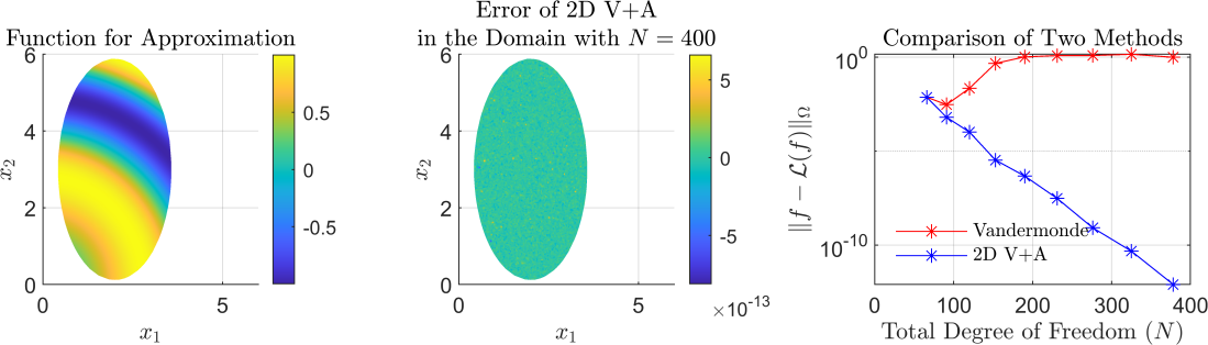
Figure 4: Approximating $f(x_{(1)},x_{(2)})=\sin(\frac{x_{(1)}^{2}+x_{(2)}^{2}+x_{(1)}x_{(2)}}{5})$ on an elliptical domain (Domain $4$ in Figure 12) using randomized mesh with $M=N^{2}\log N$.

In the left plot of Figure 5, we compare the V+A approximation with the Vandermonde approximation on bounding tensor domains (V+bounding tensor). In V+bounding tensor approximation, we enclose the irregular domain in a hypercube domain, $\Omega\subset\Omega_{cube}$, and create an orthonormal Vandermonde basis on the bounding tensor-product domain. This is a common technique used in polynomial frame approximations and V+bounding tensor approximation is one of the simplest examples of frame approximations. Using the same number of sample points $M=N^{2}\log N$, V+bounding tensor approximation is less accurate than the V+A approximation at all degrees. This is because, in V+bounding tensor approximation, the sample points used are distributed on the whole tensor-product domain $\Omega_{cube}$. Only $\sim 59.59\%$ sample points are inside the domain $\Omega$, while in the V+A approximation, all sample points used are within $\Omega$ and contribute to the approximation.

Even if we increase the number of sample points for V+bounding tensor with $M=\frac{1}{0.5959}N^{2}\log N$ such that we have approximately the same number of sample points within $\Omega$, V+bounding tensor approximation with more sample points still gives a worse approximation than the V+A method. This is because the orthonormal basis generated in V+bounding tensor approximation is for the bounding tensor product domain. But when restricted to an irregular subdomain, an orthonormal basis is no longer orthogonal. Numerical computations experience potential difficulties, due to the near-linear dependence of the truncated approximation system. This difficulty is also discussed in polynomial frame approximation which also uses the orthogonal polynomials on a bounding tensor product domain. There is an extensive literature in the field of frame theory to work around this difficulty; for instance, a well-conditioned approximation can be obtained via regularization [1]. More details on the frame approximation are in [2, 3, 1].

Last but not least, we test V+A approximation on a non-differential function $f(x_{(1)},x_{(2)})=|x_{(1)}-2||x_{(2)}-3|$ in the irregular domain. We found that the error reduction for the non-smooth function is much slower than the error reduction for the smooth function (Figure 5). The slow convergence in the error reduction is not caused by the V+A method; it is because polynomials are not great for approximating non-smooth functions. In other words, no polynomials in the space $\mathcal{P}^{d}_{n}$ can give a high rate of error reductions while approximating the non-differential functions as $N$ increases. Additionally, the smoothness requirement of the function is stricter for higher dimensional domains. As we observe from the right plot of Figure 5, the 2D least-squares approximation of a non-smooth function exhibits a slower error reduction than the 1D least-squares approximation of a non-smooth function. The theoretical results for convergence and explanations of these phenomena are discussed in the next section.

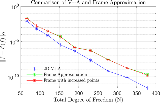
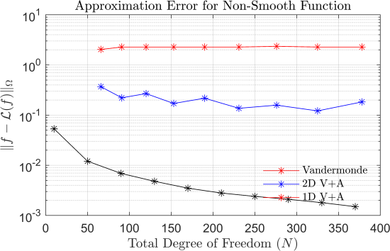
Figure 5: Left: Comparison of frame approximation and V+A Approximation for $f(x_{(1)},x_{(2)})=\sin(\frac{x_{(1)}^{2}+x_{(2)}^{2}+x_{(1)}x_{(2)}}{5})$ on an elliptical domain (Domain $4$ in Figure 12) using randomized mesh. Right: Approximating non-smooth function $f(x_{(1)},x_{(2)})=|x_{(1)}-2||x_{(2)}-3|$ on an elliptical domain and $f(x)=|x-2|$ in $[0,4]$.

4 Sample Complexity and Convergence of Multivariate V+A

Recall that in Section 2.3, we showed that the deviation from the minimax approximant in the V+A least-squares approximation (i.e. the error in the V+A least-squares approximation) can be controlled by the size of the discrete orthogonal polynomials. We also showed that the size of the discrete orthogonal polynomials can be controlled by the size of the continuous orthogonal polynomials, given enough sample complexity.

In simple domains (e.g., real intervals or tensor product domains), we know that the continuous orthogonal polynomials with respect to uniform measure are the Legendre polynomials and the continuous orthogonal polynomials with respect to Chebyshev points are the Chebyshev polynomials. Therefore, we can use the properties of these polynomials to find the sample complexity requirement and induce an error bound for V+A approximation.

However, for a general $d$-dimensional domain, the continuous orthogonal basis is in general unknown. In this section, we introduce a general approach known as admissible mesh [10, 34] to develop two near-optimal sampling methods (i.e., deterministic equispaced mesh and randomized mesh). We prove that, in many domains, using $M=\mathcal{O}(N^{2})$ equispaced points or $M=\mathcal{O}(N^{2}\log N)$ random sample points, the V+A approximant with $N$-degrees of freedom is near-optimal. Moreover, we prove that, when the sample complexity condition is satisfied, the error of the V+A approximation converges at a spectral rate with the maximum polynomial degree $n$. More specifically,

$$\|f-\mathcal{L}(f)\|_{\Omega}={o}(n^{d-k})$$ (4.1)

where $\|f-\mathcal{L}(f)\|_{\Omega}$ is the error of the V+A approximation, $d$ is the dimension of the variables (i.e., $x\in\mathbb{R}^{d}$), and $k$ is the highest order of derivative of $f$ that exists and is continuous (i.e., smoothness).

4.1 Choice of sample points

Deterministic sample points: Let $\Omega\in\mathbb{R}^{d}$ be a compact set. Let ${\boldsymbol{X}}=\{\boldsymbol{x}_{i}\}_{1\leq i\leq M}$ be a set of $M$ distinct sample points, and $f(\boldsymbol{x}_{i})$ be bounded for $1\leq i\leq M$, then there exists a unique polynomial $\mathcal{L}(f)\in\mathcal{P}^{d}_{n}$ that satisfies the least-squares system in (2.1) [10, Thm 1]. We define a linear map $\mathbb{P}_{d}$: $p\rightarrow p|_{\boldsymbol{X}}$ where $p|_{\boldsymbol{X}}$ denotes the restriction of $p$ to ${\boldsymbol{X}}$. $\mathbb{P}_{d}$ is one-to-one, bounded and continuous [10]. Thus, for each $\boldsymbol{X}$ and $\mathcal{P}^{d}_{n}$, there exists a (smallest) constant $C(\boldsymbol{X},\Omega)$ such that

$$\|p\|_{\Omega}\leq C(\boldsymbol{X},\Omega)\|p\|_{\boldsymbol{X}},\qquad\forall p\in\mathcal{P}^{d}_{n}.$$ (4.2)

$C(\boldsymbol{X},\Omega)$ depends on the distribution and the number of sample points, the degree of the polynomial $n$ and the polynomial space $\mathcal{P}^{d}_{n}$. $\boldsymbol{X}$ is called an admissible mesh if $C(\boldsymbol{X},\Omega)$ is bounded as $N$ grows. The full definition of the admissible mesh is in Appendix C.

We use Theorem 2 to control the size of $C(\boldsymbol{X},\Omega)$ (i.e., construct an admissible mesh). The proof of this theorem can be found in [10, Thm 5].

Theorem 2.

Let $p(x)\in\mathcal{P}^{d}_{n}$ be a $d$-dimensional and degree-$n$ multivariate polynomial. Let the domain $\Omega\in\mathbb{R}^{d}$ be a compact set that admits the Markov inequality,

$$\|D^{\boldsymbol{\alpha}}p\|_{\Omega}\leq{C_{M}}^{|\boldsymbol{\alpha}|}[\text{deg}(p)]^{r|\boldsymbol{\alpha}|}\|p\|_{\Omega},$$ (4.3)

where $C_{M},r$ are positive constants, $D^{\boldsymbol{\alpha}}p:=\frac{\partial^{\alpha_{1}}}{\partial{x_{(1)}}}\dotsc\frac{\partial^{\alpha_{d}}}{\partial{x_{(d)}}}p$ is the total derivative and $\boldsymbol{\alpha}:=(\alpha_{1},\dotsc,\alpha_{d})$ is the multi-index with $|\alpha|=\alpha_{1}+\dotsc+\alpha_{d}$. Let $\boldsymbol{X}=\{x_{i}\}_{1\leq i\leq M}$ be a mesh that satisfies the property

$$\text{for every ${z}\in\Omega$, there exists an $x_{i}\in\boldsymbol{X}$ such that }\|{z}-x_{i}\|_{\infty}\leq\frac{2c_{1}}{C_{M}n^{r}}$$ (4.4)

where $c_{1}$ is a constant chosen to be small enough such that $2Nc_{1}e^{Nc_{1}}<1$. Then, $\boldsymbol{X}$ is an admissible mesh. The cardinality of $\boldsymbol{X}$ is $\mathcal{O}(n^{dr})=\mathcal{O}(N^{r})$.

Remark 1.

Theorem 2 provides us with a way to discretize the domain and choose sample points that can control the size of the discrete orthogonal polynomial. For $\Omega\in\mathbb{R}^{d}$, we enclose $\Omega$ in a $d$-dimensional hypercube $\Omega_{cube}\in\mathbb{R}^{d}$. We then cover $\Omega_{cube}$ with equispaced grids dense enough such that the condition in (4.4) is satisfied. This gives us $\mathcal{O}(n^{dr})=\mathcal{O}(N^{r})$ number of nodes for the admissible mesh. Note that the deterministic sampling method can be further improved in two ways. Firstly, instead of sampling in the hypercube domain $\Omega_{cube}$. One could sample directly on $\Omega$ using rejection sampling. Details on the randomized sampling method are discussed in Theorem 3. Secondly, instead of taking equispaced samples, we can choose a set of sample points with a ‘near-optimal weight’. Details on near-optimal sampling strategy are discussed in Section 5.

There are plenty of real domains that satisfy the Markov inequality (4.3). We give a few examples following [10].

• Intervals in $\mathbb{R}$ satisfy the Markov property with $r=2$. We can form an admissible mesh of cardinality $M=\mathcal{O}(n^{2})$ with equispaced sample points.

• A convex body or unions of finite convex bodies in $\mathbb{R}^{d}$ satisfy the Markov property with $r=2$. We can form an admissible mesh of cardinality $M=\mathcal{O}(n^{2d})=\mathcal{O}(N^{2})$ with equispaced sample grids.

Random sample points: In a high-dimensional domain of which we have no explicit knowledge, it is sometimes easier to generate sample points randomly from the domain by rejection sampling. We prove that with $\mathcal{O}(N^{2}\log N)$ random sample points generated i.i.d. from a uniform measure, we can also form the admissible mesh with high probability.

Theorem 3.

Suppose that $\Omega$ satisfies the condition (4.3) in Theorem 2 and $\boldsymbol{X}$ satisfies (4.4). Then, $\boldsymbol{X}$ is a deterministic admissible mesh with cardinality $M$. Let $\boldsymbol{\tilde{X}}=\{\tilde{\boldsymbol{x}}_{1},\tilde{\boldsymbol{x}}_{2},\dotsc,\tilde{\boldsymbol{x}}_{\tilde{M}}\}$ be a set of points independently and uniformly sampled from $\Omega$. If ${\tilde{M}}\geq(c_{r}+1)M\log(M)$, where $c_{r}$ is some positive constant, then $\boldsymbol{\tilde{X}}$ is an admissible mesh with probability at least $1-M^{-c_{r}}$.

Proof.

We prove this theorem using a similar approach to [34, Thm 4.1]. We aim to show that with sufficiently large $\tilde{M}$, $\boldsymbol{\tilde{X}}$ satisfies the condition in (4.4) with high probability. For notational simplicity, we denote $E:=\frac{c_{1}}{C_{M}n^{r}}$ and rewrite the condition in (4.4) as $\boldsymbol{X}\cap\bar{B}_{E}(\boldsymbol{x})\neq\varnothing$ for all $\boldsymbol{x}\in\boldsymbol{X}$, where $\bar{B}$ denotes the closed ball with center $\boldsymbol{x}$ and radius $E$. Since $\{\tilde{\boldsymbol{x}}_{i}\}_{1\leq i\leq\tilde{M}}$ are i.i.d. samples from the uniform distribution, we have,

$$\mathbb{P}\left[\boldsymbol{\tilde{X}}\cap\bar{B}_{E}(\boldsymbol{x})\neq\varnothing\right]=1-\big{(}\mathbb{P}\left[\boldsymbol{\tilde{x}}_{1}\cap\bar{B}_{E}(\boldsymbol{x})=\varnothing\right]\big{)}^{\tilde{M}}\geq 1-\left(1-M^{-1}\right)^{\tilde{M}}\geq 1-e^{\tilde{M}/M}.$$

By taking $\tilde{M}=(c_{r}+1)M\log(M)$ with $c_{r}>0$, we achieve $\boldsymbol{\tilde{X}}\cap\bar{B}_{E}(\boldsymbol{x})\neq\varnothing$ with probability at least $1-M^{-{c_{r}}}$. Applying Theorem 2 completes the proof. ∎

Assuming $\Omega\in\mathbb{R}^{d}$ satisfies the Markov inequality in (4.3) with constant $C_{M}$ and $r=2$, by Theorem 2 and Theorem 3, there exists a randomized admissible mesh with cardinality $M=\mathcal{O}(N^{2}\log N)$. This explains the sample complexity we use in Figure 4.

4.1.1 Related Work on Sample Complexity

In this subsection, we discuss the difference in construction between the sample complexity of V+A approximation and the sample complexity of polynomial frame approximation.

There are many existing proofs for the sample complexity of polynomial approximations [2, 3, 11, 12, 24]. For instance, in [11, 12], the proof by Cohen et al. first constructs a $\mathcal{L}^{2}$-continuous orthogonal basis $\{J_{1},J_{2},\dotsc,J_{N}\}$, such that $\int_{\Omega}J_{i}(x)J_{j}(x)dx=\delta_{i,j}.$ Then, the solution of their least-squares problem can be computed by solving the $M\times M$ Gram matrix system, $\boldsymbol{Q}_{1}^{*}\boldsymbol{Q}_{1}d_{1}=f$ where the $(i,j)$th entries of $\boldsymbol{Q}_{1}$ is $J_{j}(x_{i})$ for $1\leq j\leq N$ and $1\leq i\leq M$. The purpose of their analysis is to find how many sample points we need such that the discrete measure inherits the orthogonality of $\{J_{i}\}_{1\leq i\leq N}$. Namely, how to choose $M$ such that

$$\sum_{i=1}^{M}{J_{j}(x_{i})J_{k}(x_{i})}\approx\delta_{j,k}\qquad\text{and}\qquad\mathbb{E}(\boldsymbol{Q}_{1}^{*}\boldsymbol{Q}_{1})\approx\boldsymbol{I}_{n}.$$

Using the exponentially decreasing bounds on tail distributions $\mathbb{P}(\|\boldsymbol{Q}_{1}^{*}\boldsymbol{Q}_{1}-I\|\geq\frac{1}{2})$, Cohen et al. proved that $M=\mathcal{O}(N^{2}\log N)$ random sample points is enough to obtain a stable least-squares approximation.

In [3], Adcock and Huybrechs give different proof for the sample complexity of frame approximation on irregular domains. As opposed to admissible mesh, the key step of the proof uses the Nikolskii inequality [23] on the bounding tensor-product domain

$$\|p\|_{\Omega_{cube}}\leq\mathcal{N}\|p\|_{\mathcal{L}^{2}(\Omega_{cube})}$$ (4.5)

where $\mathcal{N}$ is a constant that depends on the domain and the sample complexity. They proved that the least squares are near-optimal if the domain satisfies the $\lambda$-rectangle property. Namely, the bounding domain can be written as a (possibly overlapping and uncountable) union of hyperrectangles $\Omega_{cube}$ where $\lambda$ is the value of $\text{Volume}(\Omega)/\text{Volume}(\Omega_{cube})$. The sample complexity required scales by $N^{2}\lambda^{-1}$ where $N$ is the total degree of freedom.

Although sample complexity results obtained for polynomial frame approximation and for V+A approximation are similar, the idea and the construction of the proof is different. Firstly, in polynomial frame approximation, the proof starts with a continuous orthogonal polynomial and explores the distribution of sample points such that the discrete least-squares matrix is approximately orthogonal (i.e., $\boldsymbol{Q}_{1}^{*}\boldsymbol{Q}_{1}\approx I_{n}$). By construction in V+A, we start with a discrete orthogonal basis (i.e., $\boldsymbol{Q}^{*}\boldsymbol{Q}=I_{n}$) and examine the behaviours of these discrete orthogonal polynomials in the domain. Another difference is that these two approaches are building the bound using different norm spaces in different domains. In V+A, we use the suprema of discrete orthogonal polynomials, $\|p\|_{\boldsymbol{X}}$, while in the polynomial frame approach, the Nikolskii inequality uses the $\mathcal{L}_{2}$ norm, $\|p\|_{\mathcal{L}^{2}(\Omega_{cube})}$. Lastly, there is also a difference in the sample complexity’s dependence on the domain. The sample points used by V+A do not require information on the bounding domain and, as such, are independent of the ratio $\text{Volume}(\Omega)/\text{Volume}(\Omega_{cube})$.

4.2 Stability and Accuracy of Multivariate Vandermonde with Arnoldi

Theorem 4 shows that, under a suitable sample complexity, the error of the V+A least-squares approximant scales polynomially with the error of the best least-squares approximant. Along with multiple numerical examples, we also analyze the convergence rate and error bound for the V+A least-squares approximations.

Theorem 4.

Let $f:\Omega\rightarrow{\mathbb{R}^{d}}$ be a continuous multivariate function. The domain $\Omega\in\mathbb{R}^{d}$ is compact and admits the Markov inequality with $r=2$. We choose $M=\mathcal{O}(N^{2})$ equispaced sample points $\boldsymbol{X}$ from $\Omega$ using the sampling method in Remark 1. $\mathcal{L}$ denotes the V+A least-squares operator with $N$ degrees of freedom using sample points $\boldsymbol{X}$ from the domain $\Omega$. Then,

$$\|f-\mathcal{L}(f)\|_{\Omega}\leq\left(1+\frac{1}{M}C(\boldsymbol{X},\Omega)\|\boldsymbol{Q}\boldsymbol{Q}^{*}\|_{\infty}\right)\|f-p^{*}\|_{\Omega}\leq(1+\mathcal{O}(N))\|f-p^{*}\|_{\Omega}$$ (4.6)

where $p^{\ast}\in\mathcal{P}^{d}_{n}$ is the best polynomial approximation of $f$.

Proof.

. Denote $g:=\|f-p^{*}\|$. By the triangle inequality, we have

$$\|f-\mathcal{L}(f)\|_{\Omega}\leq\|f-p^{\ast}\|_{\Omega}+\|\mathcal{L}(p^{\ast}-f)\|_{\Omega}=\|g\|_{\Omega}+\|\mathcal{L}(g)\|_{\Omega}.$$ (4.7)

Since $\mathcal{L}(g)\in\mathcal{P}^{d}_{n}$, we write it as a linear combination of discrete orthogonal polynomials $\mathcal{L}(g):=\sum_{j=1}^{N}\beta_{j}\phi_{j}=\boldsymbol{Q}\boldsymbol{\beta}$ where $\boldsymbol{\beta}:=[\beta_{1},\dotsc,\beta_{N}]^{T}\in\mathbb{R}^{N}.$ According to (2.9), $\boldsymbol{\beta}=\frac{1}{M}\boldsymbol{Q}^{*}\tilde{g}$. Using the definition of $C(\boldsymbol{X},\Omega)$, we have

$$\|\mathcal{L}(g)\|_{\Omega}\leq C(\boldsymbol{X},\Omega)\|\mathcal{L}(g)\|_{\boldsymbol{X}}=C(\boldsymbol{X},\Omega)\|\boldsymbol{Q}\boldsymbol{\beta}\|_{\infty}=\frac{1}{M}C(\boldsymbol{X},\Omega)\|\boldsymbol{Q}\boldsymbol{Q}^{*}\tilde{g}\|_{\infty}.$$ (4.8)

Substituting (4.8) into (4.7) gives the first inequality in (4.6). Using matrix property $\frac{1}{M}\|\boldsymbol{Q}\boldsymbol{Q}^{*}\|_{\infty}<\frac{1}{\sqrt{M}}\|\boldsymbol{Q}\boldsymbol{Q}^{*}\|_{2}=\sqrt{M}$ and the sample complexity assumption $M=\mathcal{O}(N^{2})$, we arrive at the second inequality in (4.6). ∎

Remark 2.

A similar bound was derived by Calvia and Levenberg in [10, Thm 2] using Hermitian inner product norm,

$$\|f-\mathcal{L}(f)\|_{\Omega}\leq\bigg{(}1+(1+\sqrt{M})C(\boldsymbol{X},\Omega)\bigg{)}\|f-p^{\ast}\|_{\Omega}.$$ (4.9)

Since $\frac{1}{M}\|\boldsymbol{Q}\boldsymbol{Q}^{*}\|_{\infty}<\frac{1}{\sqrt{M}}\|\boldsymbol{Q}\boldsymbol{Q}^{*}\|_{2}=\sqrt{M}$, it is straightforward to verify that our bound in Theorem 4 gives a sharper approximation than the bound in (4.9) by Calvia and Levenberg.

In fact, due to the special properties of the V+A basis (i.e., $\boldsymbol{Q}$), our numerical results suggest that V+A approximant converges at an even faster rate than the bound in Theorem 4. The rate of convergence is

$$\|f-\mathcal{L}(f)\|_{\Omega}\approx(1+\sqrt{2N})\|f-p^{*}\|_{\Omega}.$$ (4.10)

Namely, with $M=N^{2}$ equispaced sample points, $\frac{1}{M}\|\boldsymbol{Q}\boldsymbol{Q}^{*}\|_{\infty}$ actually scales like $\sqrt{2N}$ in many regions (Figure 6).

Let us give a brief justification of why this should be the case. First, we rewrite $\frac{1}{M}\|\boldsymbol{Q}\boldsymbol{Q}^{*}\|_{\infty}$ in expanded form

$$\frac{1}{M}\max_{1\leq k\leq M}\sum_{i=1}^{M}\left|\sum_{j=1}^{N}{\phi_{j}(\boldsymbol{x}_{k})}\phi_{j}(\boldsymbol{x}_{i})\right|\leq\underbrace{\left(\max_{1\leq j\leq N,1\leq k\leq M}|{\phi_{j}(\boldsymbol{x}_{k})}|\right)}_{:=Q_{\max}}\underbrace{\left(\frac{1}{M}\sum_{i=1}^{M}\left|\sum_{j=1}^{N}\phi_{j}(\boldsymbol{x}_{i})\right|\right)}_{:=S_{N}}.$$

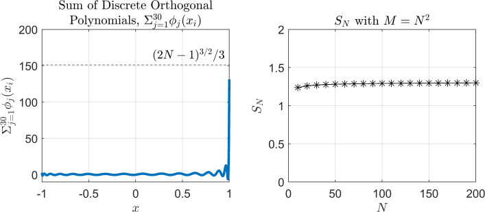
Figure 14: Left: Size of $\sum_{j=1}^{30}\phi_{j}(\boldsymbol{x}_{i})$ in $[-1,1]$. Right: Size of $\frac{1}{M}\sum_{i=1}^{M}\left|\sum_{j=1}^{N}\phi_{j}(\boldsymbol{x}_{i})\right|$ as $N$ increases with $M=N^{2}$.

In real intervals, since the discrete orthogonal polynomials are well approximated by the scaled Legendre polynomial as illustrated by (2.12), thus $Q_{\max}\approx\sqrt{2N-1}$ with $M=\mathcal{O}(N^{2})$ equispaced points. On the other hand, $\sum_{j=1}^{N}\phi_{j}(\boldsymbol{x}_{i})$ is small in the majority of the interval and only takes large values near the endpoints (Figure 14 in Appendix D). The supremum of $\sum_{j=1}^{N}\phi_{j}(\boldsymbol{x}_{i})$ has a scaling of $\sum_{j=1}^{N}\sqrt{2j-1}\approx\frac{(2N-1)^{3/2}}{3}$ in an interval of length $M^{-1}$. The mean value of the absolute sum of the discrete orthogonal polynomials, $S_{N}$, is relatively constant as $N$ grows. Our numerical experiment shows that $S_{N}\in[1.2,1.3]$ when $N$ increases from $10$ to $300$ (Appendix D). Therefore, $Q_{\max}S_{N}$ together gives an upper bound for $\frac{1}{M}\|\boldsymbol{Q}\boldsymbol{Q}^{*}\|_{\infty}$, that is, $\mathcal{O}(\sqrt{2N-1})$. Similar arguments follow for the 2D domains and the bound in 2D is obtained using $\max_{j,k}|{\phi_{j}(\boldsymbol{x}_{k})}|\approx\sqrt{2N}.$

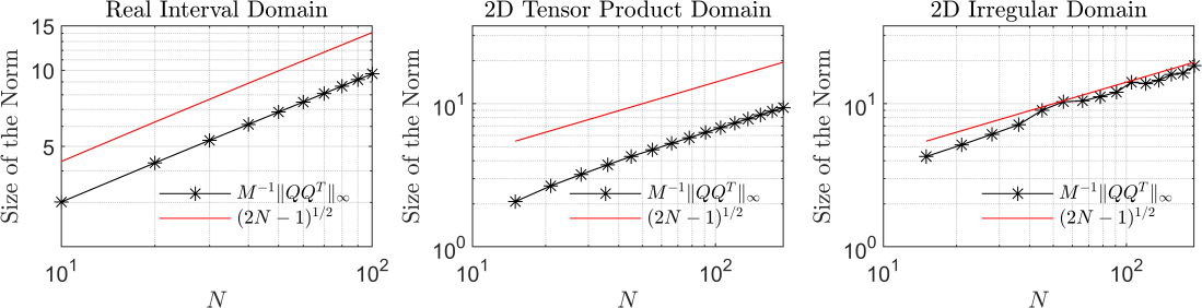
Figure 6: Size of $\frac{1}{M}\|\boldsymbol{Q}\boldsymbol{Q}^{*}\|_{\infty}$ in different domains. The left two plots are generated with $M=N^{2}$ equispaced sample points in $[-1,4]$ and $[-1,4]\times[-1,6]$, respectively. The right plot is generated with $M=N^{2}\log N$ random sample points on an elliptical domain (Domain $4$ in Figure 12).

Convergence Rate and Error Bound: Using the bound in (4.6), we can deduce the rate of convergence of the V+A approximation given enough sample points as the degree increases. Let $\Omega\in\mathbb{R}^{d}$ be a compact set and $f\in\mathcal{C}^{k}(\mathbb{R}^{d})$. Jackson’s Theorem [5] gives a bound for the best minimax approximation error

$$\|f-p^{\ast}\|_{\Omega}={o}(n^{-k}),\qquad n\rightarrow\infty$$ (4.11)

where $p^{\ast}$ is the best polynomial approximation in $\mathcal{P}^{d}_{n}$. Assume that $\Omega\in\mathbb{R}^{d}$ satisfies the Markov inequality (4.3) with $r=2$ and the admissible mesh has $M=\mathcal{O}(n^{2d})=\mathcal{O}(N^{2})$ equispaced sample points, then using the estimate in (4.6), we have

$$\|f-\mathcal{L}(f)\|_{\Omega}\leq(1+\mathcal{O}(N)){o}(n^{-k})={o}(n^{d-k})={o}(N^{1-\frac{k}{d}})$$ (4.12)

where $n$ is the maximum degree of the polynomial and $N$ is the total degree of freedom. The bound in (4.12) asserts that the convergence is at a spectral rate depending on the smoothness of $f$ in $\Omega$. It also exhibits the familiar curse of dimensionality. Namely, for functions with the same smoothness $k$, the least-squares approximations converge slower for higher dimensions $d$.

Numerically, we test the V+A algorithm for functions of specific smoothness in 1D and in 2D. For smoothness $k=0,1,2,\infty$ and dimension $d=1,2$, let

$$f_{k}(\boldsymbol{x}):=\sum_{r=1}^{d}|x_{(r)}|^{2k+1}\text{ where }\boldsymbol{x}=(x_{(1)},\dotsc,x_{(d)})\in[-1,1]^{d}.$$ (4.13)

We also set $f_{\infty}(\boldsymbol{x}):=\sum_{r=1}^{d}\sin[\exp({x_{(r)}})\cos(x_{(r)})]$. Clearly, $f_{k}\in\mathcal{C}^{k}([-1,1]^{d})$ for $k=0,1,2,\infty$.

For fixed $n$, $d$, and $\boldsymbol{X}$, the term $C(\boldsymbol{X},\Omega)\frac{1}{M}\|\boldsymbol{QQ}^{T}\|$ is the same for all functions. Thus, the improvement in convergence rates of the smoother functions comes from the best minimax approximation error terms $\|f-p^{\ast}\|_{\Omega}$. Since $\frac{1}{M}\|\boldsymbol{QQ}^{T}\|_{\infty}\sim\mathcal{O}(\sqrt{N})$ for tensor-product domains, the least-squares approximations of $f_{1}$ and $f_{2}$ converge like ${o}(n^{-3/2})$ and ${o}(n^{-7/2})$ in 1D and ${o}(n^{-1})$ and ${o}(n^{-3})$ in 2D, respectively. The convergence rates of the four bivariate functions are approximately the square root of the convergence rates of the univariate counterparts. This is expected as we only have $\sim\sqrt{N}$ degrees of freedom in the $x_{(1)}$ or the $x_{(2)}$ directions for the bivariate approximation. As a result, the best minimax approximation error can only decrease at a rate of ${o}({N}^{-\frac{k}{2}})={o}(n^{-k})$.

figurec

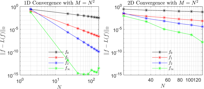
Figure 7: The set of sample points $\boldsymbol{X}=\{x_{i}\}_{1\leq i\leq N^{2}}$ and evaluation points $\boldsymbol{Y}=\{y_{i}\}_{1\leq i\leq 10N^{2}}$ are chosen as equispaced points. The domain for approximation is $[-1,1]$ in 1D and $[-1,1]^{2}$ in 2D.

4.3 Relationship between Lebesgue Constant and Admissible Mesh

The bound in Theorem 4 involving $C(\boldsymbol{X},\Omega)$ is analogous to the bound in Theorem 1 involving $\Lambda_{\boldsymbol{X}}$. Van Barel and Humet [31] proved that $C(\boldsymbol{X},\Omega)\leq\Lambda_{\boldsymbol{X}}$ for $M\geq N$, with equality in the case of interpolation ($M=N$). That said, the relationship between the bound in Theorem 4 and the bound in Theorem 1 appears to be unknown in the literature. Computing an upper bound for $C(\boldsymbol{X},\Omega)$ in a general domain is analytically difficult. This is because the size of $C(\boldsymbol{X},\Omega)$ depends on the constants $C_{M}$ and $r$ in the Markov inequality and, thus, is domain-dependent. In this section, we compute the upper bounds of $C(\boldsymbol{X},\Omega)$ for tensor-product domains and use these as examples to illustrate that the bound in Theorem 4 and the bound in Theorem 1 are comparable in size.

Lemma 5.

Let $\Omega=[-1,1]$. Fix any $N\in\mathbb{N}$, if we sample $M=N^{2}$ equispaced sample points $\boldsymbol{X}$ from $\Omega$, then $\|p\|_{\Omega}\leq C(\boldsymbol{X},\Omega)\|p\|_{\boldsymbol{X}}$ and $C(\boldsymbol{X},\Omega)\leq 2$.

Proof.

. By Markov inequality in $[-1,1]$ is $\|p^{\prime}\|_{\Omega}\leq\deg(p)^{2}\|p\|_{\Omega}$ for all $p\in\mathcal{P}^{1}_{n}$ [10, 33]. By the mean value theorem, for all $i=1,\dotsc,M-1$ and $x\in(x_{i},x_{i+1})$,

$$\exists\xi\in(x_{i},x_{i+1})=:I_{i},\text{ such that }p(x)-p(x_{i})=(x-x_{i})p^{\prime}(\xi).$$ (4.14)

Taking the supremum over $\Omega$ is equivalent to taking the maximum of the supremum in each subintervals $I_{i}$. Thus we have,

$$\max_{1\leq i\leq M-1}\|p(x)-p(x_{i})\|_{I_{i}}\leq\max_{1\leq i\leq M-1}\|{x-x_{i}}\|_{I_{i}}\|p^{\prime}(\xi)\|_{\Omega}\leq(2M)^{-1}{N^{2}}\|p\|_{\Omega},$$ (4.15)

where the last inequality uses the Markov inequality. It also uses the property of the equispaced mesh that $|{x-x_{i}}|\leq(2M)^{-1}$ for all $x\in I_{i}$ and all $i=1,\dotsc,M-1$. Applying the triangle inequality, we have

$$\|p\|_{\Omega}=\max_{1\leq i\leq M}\|p(x)-p(x_{i})+p(x_{i})\|_{I_{i}}\leq\max_{1\leq i\leq M}\|p(x)-p(x_{i})\|_{I_{i}}+\|p\|_{\boldsymbol{X}}$$ (4.16)

and consequently

$$\|p\|_{\Omega} \leq\frac{1}{1-N^{2}(2M)^{-1}}\|p\|_{\boldsymbol{X}}=2\|p\|_{\boldsymbol{X}},\qquad\forall N=1,2\dotsc\text{ with }M=N^{2}.$$ (4.17)

Thus, $C(\boldsymbol{X_{1D}},[-1,1])\in(1,2]$ where $\boldsymbol{X_{1D}}$ denotes the equispaced points in $[-1,1]$. ∎

The results in (4.15)-(4.17) can be extended to higher dimensional tensor-product domains. Let $\boldsymbol{X_{2D}}$ be an equispaced mesh in $[-1,1]^{2}$ with $M=N^{2}$ sample points and $\{\boldsymbol{I}_{i}\}_{1\leq i\leq M}$ denote the sub-grids of the mesh. In the square equispaced mesh, we have $\max_{1\leq i\leq M}\|\boldsymbol{x}-\boldsymbol{x}_{i}\|_{\boldsymbol{I}_{i}}\leq(\sqrt{2}M)^{-1}$, and thus $C(\boldsymbol{X_{2D}},[-1,1]^{2})\in(1,2+\sqrt{2}]$.

We plot the upper and lower bounds of $\frac{1}{M}C(\boldsymbol{X},\Omega)\|\boldsymbol{Q}\boldsymbol{Q}^{*}\|_{\infty}$ as the dotted lines in Figure 8. We find that $\frac{1}{M}C(\boldsymbol{X},\Omega)\|\boldsymbol{Q}\boldsymbol{Q}^{*}\|_{\infty}$ is of the same order of magnitude as the Lebesgue constant. This numerical result illustrates that even though we used two approaches to deduce the bound in Theorem 4 and the bound in Theorem 1, these two bounds are of the same order of magnitude in many domains.

figurec

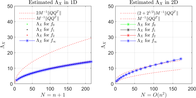
Figure 8: $\Lambda_{\boldsymbol{X}}$ are computed for the four functions in (4.13). The Lebesgue constants for the four functions are the same at all degrees. This confirms the theoretical result that $\Lambda_{\boldsymbol{X}}$ is independent of the function that we are approximating.

5 Near-Optimal Sampling Strategy for V+A

In this section, we propose a new variant of the weighted least-squares algorithm that uses the multivariate V+A to create the discrete orthogonal basis. We refer to our V+A weighted least-squares algorithm as VA+Weight. In [1, 24, 12], the authors gave comprehensive analyses on this weighted sampling strategy and proved that only $M=\mathcal{O}(N\log N)$ sample points are needed for a well-conditioned and accurate approximation.

In VA+Weight, we use the same weighting measure as in [1]. But instead of creating the discrete orthogonal basis with QR factorization, we use V+A as the orthogonalization strategy for the Vandermonde basis. Since the Vandermonde matrix $\boldsymbol{A}$ is usually highly ill-conditioned, and computing its $Q$ factor incurs errors proportional to $\kappa_{2}(\boldsymbol{A})$ [19, Ch. 19]. Even though the QR factorization is a stable orthogonalization technique, the discrete orthogonal basis generated from $\boldsymbol{A}$ could still be inaccurate. We refer to the weighted least-squares approximation using the QR factorization as QR+Weight.

Along with multiple numerical examples, we illustrate that VA+Weight gives more accurate approximations than QR+Weight for high-degree polynomial approximations. Due to the reduced sample density, VA+Weight also gives a lower online computational cost than the unweighted V+A least-squares method. Moreover, VA+Weight acts as a practical tool for selecting the near-optimal distribution of sample points in a high-dimensional irregular domain.

In Section 5.1, we explain the algorithm and the numerical setup for the weighted least-squares approximation. We provide proof of the stability of the weighting measure for sample points. In Section 5.2, we give numerical examples to compare the VA+Weight and QR+Weight algorithms.

5.1 Weighted Least-Squares Approximation

The VA+Weight algorithm is presented in Algorithm 1 and the remarks for the algorithm are given in Remark 3. Algorithm 1 is a V+A variant of Method 1 in [1].

Input: Domain $\Omega$ and a probability measure $\rho$ over $\Omega$; Bounded and continuous $f\in\mathcal{C}(\Omega)$; $N$-dimensional polynomial space $\mathcal{P}^{d}_{n}$; Number of sample points $M$ and $\hat{M}$, with $M\geq\hat{M}\geq N$; Basis $\hat{\psi}=[\hat{\psi}_{1}(\boldsymbol{x}),\dotsc,\hat{\psi}_{N}(\boldsymbol{x})]^{T}$ for $\mathcal{P}^{d}_{n}$ (no need to be orthogonal, for instance, Vandermonde basis is enough);
Output: The coefficients $\hat{d}\in\mathbb{R}^{N}$ of the polynomial approximant.

Step 1: Draw $M$ random sample points $\boldsymbol{X}=\{\boldsymbol{x}_{i}\}_{1\leq i\leq M}\stackrel{{\scriptstyle i.i.d.}}{{\sim}}\rho$. Compute the function values at $\boldsymbol{X}$ i.e $\boldsymbol{\tilde{f}}\in\mathbb{R}^{M}$.
Step 2: Construct $M\times N$ Vandermonde matrix $\boldsymbol{A}$ with the $(i,j)$th entry as $\hat{\psi}_{j}(\boldsymbol{y}_{i})$. If $\operatorname{rank}(\boldsymbol{A})=N$, go to Step 3, else go back to Step 1.
Step 3: Apply the Multivariate V+A algorithm (Algorithm 4 in Appendix B) to $\boldsymbol{A}$ to generate $\boldsymbol{Q}\in\mathbb{R}^{M\times N},\boldsymbol{H}\in\mathbb{R}^{N\times N}$ such that $\mbox{diag}(\boldsymbol{X})\boldsymbol{Q}=\boldsymbol{Q}\boldsymbol{H}+h_{N+1,N}q_{N+1}e_{N}$.
Step 4: Define a probability distribution $\pi=\{\pi_{i}\}_{1\leq i\leq M}$ on $\{1,\dotsc,M\}$, such that $\pi_{i}=\frac{1}{\|\boldsymbol{Q}\|_{F}^{2}}\sum_{j=1}^{N}|\boldsymbol{Q}_{i,j}|^{2},$ for $i=1,\dotsc,M,$ where $\boldsymbol{Q}_{i,j}$ are the $(i,j)$th entry of $\boldsymbol{Q}$.
Step 5: Draw $\hat{M}$ integers $\{k_{1},\dotsc,k_{\hat{M}}\}$ independently from $\pi$. Define $\hat{\boldsymbol{Q}}$ and $\boldsymbol{\hat{f}}$ as the corresponding scaled rows of $\boldsymbol{Q}$ and $\boldsymbol{\tilde{f}}$, such that the point-wise entries are

$$\hat{\boldsymbol{Q}}_{i,j}:=\frac{\boldsymbol{Q}_{k_{i},j}}{\sqrt{\hat{M}M\pi_{k_{i}}}},\qquad\boldsymbol{\hat{f}}_{i}:=\frac{f(\boldsymbol{x}_{k_{i},j})}{\sqrt{\hat{M}M\pi_{k_{i}}}},\qquad i=1,\dotsc,\hat{M},\quad j=1,\dotsc,N.$$

Step 6: $\boldsymbol{\hat{d}}=\boldsymbol{\hat{Q}}\backslash\boldsymbol{\hat{f}}.$ Solve the least-squares problem by the MATLAB backslash command. Approximate the value of $f$ using the evaluation algorithm in Algorithm 5 and give the output.

Algorithm 1 Weighted V+A algorithm (VA+Weight)

Remark 3.

1): We assume that it is possible to draw samples from the measure $\rho$ in Step 1. We use the uniform rejection sampling method to draw samples. We end the rejection sampler once we have enough sample points.

2): To ensure that $\operatorname{span}\{\phi_{1},\dotsc,\phi_{N}\}=\mathcal{P}^{d}_{n}$ in Step 2 of the algorithm, if $\boldsymbol{A}$ is rank deficient, we add additional sample points until $\operatorname{rank}(\boldsymbol{A})=N$.

3): The construction of $\boldsymbol{Q}$ uses the multivariate V+A algorithm (Algorithm 4 in Appendix B). Numerically, the orthogonalization algorithm is subject to a loss of orthogonality due to numerical cancellation. The numerically constructed discrete orthogonal basis is said to be $\epsilon_{m}$-orthonormal for $\epsilon_{m}>0$, namely, $\|\boldsymbol{Q}^{*}\boldsymbol{Q}-\boldsymbol{I}\|^{2}_{F}=\sum_{j,k=1}^{N}|\langle\phi_{j},\phi_{k}\rangle_{M}-\delta_{j,k}|^{2}\leq\epsilon_{m}^{2}.$ By [19, Thm 19.4] and [15, Thm 2], executing CGS twice gives us a good bound $\epsilon_{m}\sim\mathcal{O}(MN^{3/2})\boldsymbol{u}$, where $\boldsymbol{u}$ is the unit roundoff.

In Algorithm 1, $\sum_{j=1}^{N}|\boldsymbol{Q}_{i,j}|^{2}$ represents the sum of the absolute value of discrete orthogonal polynomials at the sample points. The weighting measure $\pi$ can be interpreted as choosing the sample points which maximize the absolute sum of the discrete orthogonal polynomials at the sample points. Heuristically, this weighting measure makes sense as the supremum usually happens near the boundaries and corners of the domain. Many sampling measures, such as Chebyshev points in real intervals and Padua points [7, 9] in higher dimensional tensor-product domains have highlighted the importance of sample points near the boundary and corners.

$\hat{M}$ is the number of points we selected from a total of $M$ sample points. The main question that we analyze in this section is how large $\hat{M}$ needs to be chosen in relation to $N$ to ensure a near-optimal approximation. As we will prove later, with the probability distribution defined in Step 4, a log-linear scaling of $\hat{M}=\mathcal{O}(N\log N)$ is enough for a well-conditioned, near-optimal weighted least-squares approximation (provided that $M$ is large enough). The reduced sample complexity in Algorithm 1 gives a reduced online computational cost. The computational cost for Algorithm 1 is dominated by the cost of Step 3 and Step 6, which are $\mathcal{O}(MN^{2})$ flops and $\mathcal{O}(\hat{M}N^{2})$ flops, respectively. Since we need $M=\mathcal{O}(N^{2}\log N)$ random sample points to generate a randomized admissible mesh for convex domains or unions of convex domains in $\mathbb{R}^{d}$, Algorithm 1 gives an online computational cost of $\mathcal{O}(N^{3}\log N)$ while the unweighted least-squares method described in Section 3 requires $\mathcal{O}(N^{4}\log N)$.

Algorithm 1 can be interpreted as a weighted least-squares system with V+A orthogonalization. We lay out the notation of the weighted least-squares system as follows. Consider the set $\boldsymbol{X}=\{\boldsymbol{x}_{i}\}_{1\leq i\leq M}\stackrel{{\scriptstyle i.i.d.}}{{\sim}}\rho$, we define $\tilde{\rho}$ as the discrete uniform measure on $\boldsymbol{X}$, such that $\tilde{\rho}(\boldsymbol{x}_{i})=\frac{1}{M}$ for $1\leq i\leq M$. For all $\boldsymbol{x}_{i}\in\boldsymbol{X}$, we write the weighted sampling method in Step 5 as a probability measure $\sigma$ on $\boldsymbol{X}$,

$$d\sigma(\boldsymbol{x}_{i}):=w(\boldsymbol{x}_{i})^{-1}d\tilde{\rho}(\boldsymbol{x}_{i})=\frac{1}{\upsilon}\sum_{j=1}^{N}{\phi_{j}(\boldsymbol{x}_{i})^{2}}d\tilde{\rho}(\boldsymbol{x}_{i}),\qquad\text{where }\upsilon:=\frac{\|\boldsymbol{Q}\|_{F}}{M}.$$ (5.1)

Clearly, $\int_{\Omega}d\sigma=\int_{\Omega}w^{-1}d\tilde{\rho}=1$ and $N(1-\epsilon_{m})\leq\upsilon\leq N(1+\epsilon_{m})$ due to the $\epsilon_{m}$-orthogonality. For simplicity, we use $\boldsymbol{\hat{X}}=\{\boldsymbol{\hat{x}}_{i}\}_{1\leq i\leq\hat{M}}\stackrel{{\scriptstyle i.i.d.}}{{\sim}}\sigma$ to denote $\{\boldsymbol{{x}}_{k_{i}}\}_{1\leq i\leq\hat{M}}$, where the indices $\{k_{i}\}_{1\leq i\leq\hat{M}}$ are drawn as described in Step 5. Then, the weighted least-squares estimator is

$$\boldsymbol{\hat{d}}=\operatorname*{argmin}_{\boldsymbol{{d}}\in\mathbb{R}^{N}}\|\boldsymbol{\hat{Q}d}-\boldsymbol{\hat{f}}\|_{2}\text{ or equivalently, }\mathcal{L}(f)_{W}:=\operatorname*{argmin}_{p\in\mathcal{P}^{d}_{n}}\|p-f\|_{\hat{M}}$$ (5.2)

where the notation $\langle\cdot,\cdot\rangle_{\hat{M}}$ denotes $\langle u,v\rangle_{\hat{M}}:=\frac{1}{\hat{M}}\sum_{i=1}^{\hat{M}}w(\boldsymbol{\hat{x}_{i}})u(\boldsymbol{\hat{x}}_{i})v(\boldsymbol{\hat{x}}_{i})\text{, and }\|u\|_{\hat{M}}=\sqrt{\langle u,u\rangle_{\hat{M}}}$. Using the weight matrix $\boldsymbol{\hat{W}}$, the weighted least-squares problem can be written as

$$\boldsymbol{\hat{d}}=\operatorname*{argmin}_{\boldsymbol{{d}}\in\mathbb{R}^{N}}\|\boldsymbol{\hat{W}{Q_{S}}d}-\boldsymbol{{f_{S}}}\|_{2}$$ (5.3)

where

$$\boldsymbol{\hat{W}}:=\frac{1}{\sqrt{\hat{M}}}\operatorname{diag}(\sqrt{w(\boldsymbol{\hat{x}}_{i}}))_{1\leq i\leq\hat{M}}=\frac{1}{\sqrt{\hat{M}}}\operatorname{diag}\left(\frac{1}{\sqrt{M\pi_{k_{i},j}}}\right)_{1\leq i\leq\hat{M}}.$$ (5.4)

$\boldsymbol{Q_{S}}\in\mathbb{R}^{\hat{M}\times N}$ and $\boldsymbol{f_{S}}\in\mathbb{R}^{\hat{M}}$ are the matrix and the vector formed with $\{k_{1},\dots,k_{\hat{M}}\}$ selected rows of $\boldsymbol{Q}$ and $\boldsymbol{\tilde{f}}$ in the unweighted system. $\boldsymbol{\hat{d}}:=[\hat{d}_{1},\dotsc,\hat{d}_{N}]^{T}$ is the vector of coefficients for the weighted least-squares estimator such that $\mathcal{L}(f)_{W}:=\sum_{i=1}^{N}\hat{d}_{i}\phi_{i}$. Note that $\phi_{i}$ is defined as before, namely the discrete orthogonal polynomials generated by $M$ sample points. The estimator $\mathcal{L}(f)_{W}$ is solved using normal equations, such that

$$\boldsymbol{d}=\boldsymbol{G}^{-1}(\boldsymbol{\hat{Q}^{*}\hat{f}}).$$ (5.5)

$\boldsymbol{G}:=\boldsymbol{\hat{Q}^{*}\hat{Q}}\in\mathbb{C}^{N\times N}$ is the Gram matrix which has the $(j,k)$th entry $\boldsymbol{G}_{j,k}=\langle\phi_{j},\phi_{k}\rangle_{\hat{M}}$. The vector $\boldsymbol{\hat{Q}^{*}\hat{f}}\in\mathbb{R}^{N}$ has $j$th entry $\langle\phi_{j},f\rangle_{\hat{M}}$.

Well-Conditioning of Reduced Gram Matrix: Since the weighted least-squares estimator is found by solving system (5.5) and by taking the inverse of the matrix $\boldsymbol{G}$, for stability and convergence we need to ensure that the Gram matrix $\boldsymbol{G}$ is well-conditioned. Also, we investigate how much $\boldsymbol{G}=\boldsymbol{\hat{Q}^{*}\hat{Q}}$ deviates from $\boldsymbol{{Q}^{*}{Q}}$. In other words, we want to understand whether the discrete orthogonal basis at the selected sample points $\boldsymbol{\hat{X}}$ acts as a good approximation to the discrete orthogonal basis at the full sample points $\boldsymbol{{X}}$. The following theorem adapted from [24, Thm 3] establishes these links.

Theorem 6.

For a compact, bounded domain $\Omega\in\mathbb{R}^{d}$ with the measure $\rho$, consider finding a weighted least-squares approximation in the polynomial space $\mathcal{P}^{d}_{n}$ using Algorithm 1. Assume that $\boldsymbol{X}=\{\boldsymbol{x}_{i}\}_{1\leq i\leq M}\stackrel{{\scriptstyle i.i.d.}}{{\sim}}\rho$ and the $\epsilon_{m}$-orthogonal basis are generated as described in Step 3 of Algorithm 1. For any $\hat{\alpha}\in(0,\frac{1}{2}),\epsilon_{m}\in(0,1),\hat{\delta}\in(0,1-\epsilon_{m})$, and $n\geq 1$, if the following conditions hold,

i) $$\hat{M}\geq\frac{4N(1+\epsilon_{m})}{\hat{\delta}^{2}}\log(\frac{2N}{\hat{\alpha}}),$$

ii) $$\boldsymbol{\hat{X}}=\{\boldsymbol{\hat{x}}_{i}\}_{1\leq i\leq\hat{M}}\stackrel{{\scriptstyle i.i.d.}}{{\sim}}\sigma\text{ where $\sigma$ is defined as in \eqref{sigma},}$$

then, the matrix $\boldsymbol{G}$ satisfies $\mathbb{P}(\|\boldsymbol{G}-\boldsymbol{I}\|_{2}\geq\hat{\delta}+\epsilon_{m})\leq\hat{\alpha}$ where $\boldsymbol{I}$ is the $N\times N$ identity matrix.

We give a sketch of the proof for Theorem 6. We write $\mathbb{P}(\|\boldsymbol{G}-\boldsymbol{I}\|_{2}\geq\hat{\delta}+\epsilon_{m})$ as

$$\mathbb{P}(\|\boldsymbol{G}-\boldsymbol{I}\|_{2}<\hat{\delta}+\epsilon_{m})\geq\underbrace{\mathbb{P}(\{\|\mathbb{E}(\boldsymbol{G})-\boldsymbol{I}\|_{2}<\epsilon_{m}\})}_{:=P_{1}}\underbrace{\mathbb{P}(\{\|\boldsymbol{G}-\mathbb{E}(\boldsymbol{G})\|_{2}<\hat{\delta}\})}_{:=P_{2}}.$$

The first probability term $P_{1}$ is bounded using condition $(ii)$, the equality $\mathbb{E}(\boldsymbol{G}_{j,k})=\langle\phi_{j},\phi_{k}\rangle_{M}$ and the $\epsilon_{m}$-orthogonality. The second probability term $P_{2}$ is bounded using the Bernstein Inequality and condition $(i)$ which gives a tail bound for sums of random matrices. A full proof of Theorem 6 can be found in [24, Thm 3].

Theorem 6 not only ensures that $\boldsymbol{G}$ is well-conditioned with high probability but also guarantees that the weighted least-squares problem (5.5) is stable with high probability. Under the conditions of Theorem 6, we have $1-\hat{\delta}-\epsilon_{m}\leq\|\boldsymbol{G}\|_{2}\leq 1+\hat{\delta}+\epsilon_{m}$. Using that $\boldsymbol{v}^{T}\boldsymbol{G}\boldsymbol{v}=(\boldsymbol{\hat{Q}v})^{T}(\boldsymbol{\hat{Q}v})$ for all $\boldsymbol{v}\in\mathbb{R}^{N}$, it follows that

$$\|\boldsymbol{\hat{Q}}\|_{2}=\|\boldsymbol{G}\|_{2}^{1/2},\text{ and }\|\boldsymbol{G}^{-1}\|_{2}\|\boldsymbol{\hat{Q}}^{T}\|_{2}\leq\frac{\sqrt{1+\hat{\delta}+\epsilon_{m}}}{1-\hat{\delta}-\epsilon_{m}}=:C_{\hat{\delta},\epsilon_{m}}.$$ (5.6)

Thus, we arrive at the stability result $\|\boldsymbol{\hat{d}}\|_{2}=\|\boldsymbol{G}^{-1}\boldsymbol{\hat{Q}}\boldsymbol{\hat{f}}\|_{2}\leq C_{\hat{\delta},\epsilon_{m}}\|\boldsymbol{\hat{f}}\|_{2}.$ Numerical example on the growth of $\kappa_{2}(\boldsymbol{G})$ with respect to $N$ for different sampling densities $\hat{M}$ can be found in Appendix E.

To ensure the convergence of Algorithm 1, in addition to conditions $(i)$ and $(ii)$ in Theorem 6, we also require a sample density of $M=\mathcal{O}(N^{2}\log N)$ random sample points. This result is expected as we do need $M=\mathcal{O}(N^{2}\log N)$ random sample points to form an admissible mesh and to form discrete orthogonal polynomials which are well-bounded in the domain. There are a few papers that discuss the convergence for Algorithm 1, namely [1, Thm 3.1-3.5], [3, Thm 6.6] and [24, Thm 2].

5.2 Numerical Examples for Weighted V+A Algorithm

In this subsection, we compare the VA+Weight algorithm with the QR+Weight algorithm. The two algorithms use the same weights, but the QR+Weight algorithm uses the QR factorization of the ill-conditioned Vandermonde matrix to create the discrete orthogonal basis.

In Figure 9, we plot the numerical results of approximating a smooth function using VA+Weight and QR+Weight in a real interval. As shown in the left plot, both algorithms converge with $\hat{M}=\mathcal{O}(N\log N)$ number of weighted sample points. Before the ill-conditioning of $\boldsymbol{A}$ builds in, the two algorithms performed similarly as expected. Note that the error from the two approximations will not be exactly the same as we selected the weighted sample points in a non-deterministic fashion (i.e., following the probability measure $\sigma$). However, when $\kappa_{2}(\boldsymbol{A})$ grows beyond the inverse of the machine epsilon for $N>60$, the QR+Weight approximation has an error stagnating at $10^{-5}$ as illustrated in the left plot of Figure 9. Although the QR factorization and the weighted sampling method generate a well-conditioned $\boldsymbol{\hat{Q}}$ (Figure 9), the columns of $\boldsymbol{\hat{Q}}$ do not approximate the orthogonal basis in the domain (Figure 10). Thus, accuracy is lost for large $N$.

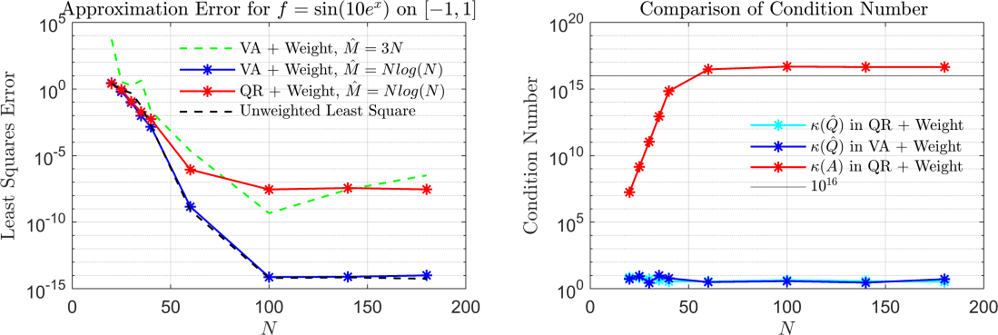
Figure 9: Comparison of VA+Weight and QR+Weight in a 1D domain. The sample points are chosen as $M=N^{2}\log N$ random points. The unweighted least-squares approximation is computed by the multivariate V+A Algorithm (i.e., Algorithm 4 in Appendix B).

On the other hand, as shown in the right plot of Figure 9, VA+Weight approximation gives a stable error reduction down to $10^{-13}$. The error reduction in VA+Weight also matches with the error reduction in the unweighted least-squares approximations. This is because the discrete orthogonal polynomials generated by V+A are unaffected by the ill-conditioning of $\boldsymbol{A}$. The value of the $30$th discrete orthogonal polynomial overlaps with the value of the $30$th scaled Legendre polynomial in the domain (Figure 10).

figurec

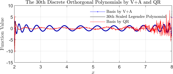
Figure 10: The discrete orthogonal polynomials and the scaled Legendre polynomials generated by VA+ Weight and QR+ Weight using $M=900$ equispaced points in $[-5,10]$.

The same patterns of convergence are found while approximating bivariate functions. As plotted in Figure 11, VA+Weight gives an approximation with higher accuracy than QR+Weight in both domains. The difference in the two approximations is less in the 2D domain than in the 1D domain. This is because the multivariate Vandermonde matrix $\boldsymbol{A}$ is, in general, less ill-conditioned in 2D domains than in 1D domains. That said, the conditioning of the multivariate Vandermonde matrix $\boldsymbol{A}$ varies greatly with the shape of the domain. VA+Weight provides a stable and generalized method for multivariate approximations in irregular domains.

Figure 11: Comparison of VA+Weight and QR+Weight in 2D domains. The sample points are chosen as $M=N^{2}\log N$ random points. We use Domain $2$ in Figure 12.

Finding the best distribution of sample points in a high-dimensional irregular domain is an open question in the literature. We highlight that the weighting method in Algorithm 1 is a practical tool for finding the near-optimal distribution of the sample points. We plot the $\hat{M}=N\log N$ sample points selected by VA+Weight for different domains in Figure 12. Notice that the selected points are clustered near corners and boundaries. This distribution pattern matches the pattern in Padua points in tensor-product domains. Note that we did not instruct the VA+Weight algorithm to place the sample points near the boundary. The algorithm naturally selected those sample points because at these points the discrete orthogonal polynomials take larger absolute values. VA+Weight shows strong adaptability in selecting near-optimal sample points in irregular domains.

Figure 12: $M=N^{2}\log N$ random sample points are drawn from the domain with $N=200$, plotted in the yellow dots. The weighted sample points selected are plotted in blue dots.

Finally, we note that different weighting measures can be used to improve different aspects of the approximation algorithm. As illustrated in the left two plots of Figure 13, the VA+Weight algorithm gives a similar accuracy as the unweighted V+A least-squares approximation but with improved efficiency. That said, the approximants obtained from VA+Weight are only near-optimal, but not the best polynomial approximation. We propose combining the multivariate V+A with Lawson’s algorithm (VA+Lawson) to obtain the best multivariate polynomial approximation. VA+Lawson is based on an iterative re-weighted least-squares process and can be used to improve the approximation accuracy. Our numerical experiments showed that through the VA+Lawson algorithm, we improved the approximation error from $1.4\times 10^{-6}$ to $3.2\times 10^{-7}$ . Moreover, we found an equioscillating error curve in 2D which is a characteristic for the best polynomial approximation [26, Thm. 24.1].

Figure 13: Approximating $f=\sin(x_{(1)}x_{(2)})$ with total degrees of freedom $N=66$ with $M=N^{2}\log N$ random sample points. We use the same domain as the middle plot of Figure 12. The error curve of the approximant using V+A, VA+Weight, VA+Lawson are plotted in the left, middle, and right plots, respectively. For VA+Lawson, we carried out $10$ Lawson’s iterations.

6 Conclusions and Perspectives

In this paper, we analyzed the multivariate Vandermonde with the Arnoldi method to approximate $d$-dimensional functions on irregular domains. V+A technique resolves the ill-conditioning issue of the Vandermonde matrix and builds the discrete orthogonal polynomials with respect to the domain. Our main theoretical result is the convergence of the multivariate V+A least-squares approximation for a large class of domains. The sample complexity required for the convergence is quadratic in the dimension of the approximation space, up to a log factor. Using a suitable weighting measure, we showed that the sample complexity can be further improved. The weighted V+A least-squares method requires only log-linear sample complexity $M=\mathcal{O}(N\log(N))$. Our numerical results confirm that the (weighted) V+A method gives a more accurate approximation than the standard orthogonalization method for high-degree approximation using the Vandermonde matrix.

V+A has many applications beyond least-squares fitting. Our numerical experiments showed that the VA+Lawson algorithm improves the approximation accuracy and generates an equioscillating error curve. Yet, the convergence profile for VA+Lawson still seems to be unknown and could be an objective of future work. Another extension under consideration involves using multivariate V+A in vector- and matrix-valued rational approximations [13, Subsec. 2.4]. Generally speaking, in any application which involves matrix operations of Vandermonde matrix (or its related form), it seems likely that the V+A procedure could be an effective idea to apply.

Appendix A Vandermonde with Arnoldi Algorithm

Input: Sample points $\boldsymbol{X}=\{{x}_{i}\}_{i=1}^{M}$, the degree $n$, $\boldsymbol{\tilde{f}}\in\mathbb{R}^{M}$.
Output: $\boldsymbol{Q}\in\mathbb{R}^{M\times N},\boldsymbol{H}\in\mathbb{C}^{N\times(N-1)}$, the coefficient of the approximation $\boldsymbol{d}\in\mathbb{R}^{N}$.
Initialize $\boldsymbol{Q}$ and $\boldsymbol{H}$ as zero matrices; Set $[\boldsymbol{Q}]_{:,1}$ as a $M\times 1$ matrix of ones.
For $l=1,2,\dotsc,n$
$\boldsymbol{v}:=\operatorname{diag}(x_{1},\dotsc,x_{M})[\boldsymbol{Q}]_{:,l};$
For $t=1,2$ (Carry out classical Gram-Schmidt twice)
$\boldsymbol{s}:=\frac{1}{M}[\boldsymbol{Q}]^{\ast}_{:,1:l}\boldsymbol{v};\quad$ $\boldsymbol{v}:=\boldsymbol{v}-[\boldsymbol{Q}]_{:,1:l}\boldsymbol{s};$
$[\boldsymbol{H}]_{1:l,l}:=[\boldsymbol{H}]_{1:l,l}+\boldsymbol{s};$
end
$[\boldsymbol{H}]_{{l+1},{l}}:=\frac{1}{\sqrt{M}}\|\boldsymbol{v}\|_{2};\quad[\boldsymbol{Q}]_{:,{l+1}}:=\boldsymbol{v}/\|\boldsymbol{v}\|_{2}$;
end
$\boldsymbol{d}=\boldsymbol{Q}\backslash\boldsymbol{\tilde{f}}.$ Solve the least-squares problem by MATLAB backslash command.

Algorithm 2 Polynomial Fitting using Univariate Vandermonde with Arnoldi [8]

Input : Evaluation points $\boldsymbol{Y}=\{{y}_{i}\}_{i=1}^{K}$, the degree $n$, $\boldsymbol{H}\in\mathbb{R}^{N\times(N-1)}$, $\boldsymbol{d}\in\mathbb{R}^{N}$;

Output: ${\boldsymbol{p}}\in\mathbb{R}^{K}$ which is the vector of values at evaluation points $\boldsymbol{Y}$.

Initialize $\boldsymbol{U}$ as a $K\times N$ zero matrix and set $[\boldsymbol{U}]_{:,1}$ as a $K\times 1$ matrix of ones;
For $l=1,2,\dotsc,n$
$\boldsymbol{v}:=\operatorname{diag}(y_{1},\dotsc,y_{K})[\boldsymbol{U}]_{:,l};$
$\boldsymbol{v}:=\boldsymbol{v}-[\boldsymbol{U}]_{:,1:l}[\boldsymbol{H}]_{1:l,l};\quad$ $[\boldsymbol{U}]_{:,l}:=\boldsymbol{v}/[\boldsymbol{H}]_{l+1,l};$
end
$\boldsymbol{{p}}:=\boldsymbol{Ud}$

Algorithm 3 Evaluating Functions for Univariate Approximation [8]

Appendix B Multivariate Vandermonde with Arnoldi Algorithm

Input: Sample points $\boldsymbol{X}=\{\boldsymbol{x}_{i}\}_{i=1}^{M}$ with $\boldsymbol{x}_{i}\in\mathbb{R}^{d}$, total degrees of freedom $N$, the index set $\mathcal{I}$ with length $N$, the function values at $\boldsymbol{X}$ i.e., $\boldsymbol{\tilde{f}}\in\mathbb{R}^{M}$.
Output: $\boldsymbol{Q}\in\mathbb{R}^{M\times N},\boldsymbol{H}\in\mathbb{R}^{N\times N}$, the coefficient $\boldsymbol{d}\in\mathbb{R}^{N}$.
Set $\boldsymbol{Q}$ and $\boldsymbol{H}$ as zero matrices; Set $[\boldsymbol{Q}]_{:,1}$ as a $M\times 1$ matrix of ones and $[R]_{1,1}=1$.
For $l=1,2,\dotsc,|\mathcal{I}|-1$
Choose the smallest $k$ such that $\exists r$ where $\mathcal{I}_{k}+\boldsymbol{e}_{r}=\mathcal{I}_{l+1}$;
$\boldsymbol{v}:=\operatorname{diag}({x_{(r)}}_{1},\dotsc,{x_{(r)}}_{M})[\boldsymbol{Q}]_{:,k};$
For $t=1,2$
       $\boldsymbol{s}:=\frac{1}{M}[\boldsymbol{Q}]^{\ast}_{:,1:l}\boldsymbol{v};\qquad$ $\boldsymbol{v}:=\boldsymbol{v}-[\boldsymbol{Q}]_{:,1:l}\boldsymbol{s};$
       $[\boldsymbol{H}]_{1:l,l+1}:=[\boldsymbol{H}]_{1:l,l+1}+\boldsymbol{s};$
       end
$[\boldsymbol{H}]_{{l+1},{l+1}}:=\frac{1}{\sqrt{M}}\|\boldsymbol{v}\|_{2};\quad[\boldsymbol{Q}]_{:,{l+1}}:=\boldsymbol{v}/\|\boldsymbol{v}\|_{2}$;
end
$\boldsymbol{d}=\boldsymbol{Q}\backslash\boldsymbol{\tilde{f}}.$ Solve the least-squares problem by MATLAB backslash command.

Algorithm 4 Polynomial Fitting using Multivariate V+A [20]

Input : Evaluation points $\boldsymbol{Y}=\{\boldsymbol{y}_{i}\}_{i=1}^{K}$ with each $\boldsymbol{y}_{i}\in\mathbb{R}^{d}$, $\mathcal{I}$, $\boldsymbol{H}\in\mathbb{R}^{N\times N}$, $\boldsymbol{d}\in\mathbb{R}\mathbb{C}^{N}$;

Output: ${\boldsymbol{p}}\in\mathbb{R}^{K}$ is the vector of values at evaluation points $\{\boldsymbol{y}_{i}\}_{i=1}^{K}$.

Initialize $\boldsymbol{U}$ as $K\times N$ zero matrix and set $[\boldsymbol{U}]_{:,1}$ as a $K\times 1$ matrix of ones;
For $l=1,2,\dotsc,|\mathcal{I}|-1$ Choose the smallest $k$ such that $\exists r$ where $\mathcal{I}_{k}+\boldsymbol{e}_{r}=\mathcal{I}_{l+1}$;
$\boldsymbol{v}:=\operatorname{diag}({y_{(r)}}_{1},\dotsc,{y_{(r)}}_{K})[\boldsymbol{U}]_{:,k};$
$\boldsymbol{v}:=\boldsymbol{v}-[\boldsymbol{U}]_{:,1:l}[\boldsymbol{H}]_{1:l,l+1};\quad$ $[\boldsymbol{U}]_{:,l+1}:=\boldsymbol{v}/[\boldsymbol{H}]_{l+1,l+1};$
end
$\boldsymbol{{p}}:=\boldsymbol{Ud}$

Algorithm 5 Evaluating Function for Multivariate Approximation [20]

Appendix C Definition of Admissible Mesh

Following  [10, 34], we give The full definition of the admissible mesh.

Definition 1.

Let $\Omega\in\mathbb{R}^{d}$ be a compact set and $\mathcal{P}^{d}_{n}$ the $d$-dimensional multivariate polynomial space with $\dim(\mathcal{P}^{d}_{n})=N$. Consider $\{\boldsymbol{X}^{(n)}\}_{n=0}^{\infty}$, a collection of subsets in $\Omega$, and assume there is a collection of constants $C(\boldsymbol{X}^{(n)},\Omega)$, such that $\forall n\geq 0$,

• $\|p\|_{\Omega}\leq C(\boldsymbol{X}^{(n)},\Omega)\|p\|_{\boldsymbol{X}}$ for all $p\in\mathcal{P}^{d}_{n}$,

• $C(\boldsymbol{X}^{(n)},\Omega)\text{ is bounded, namely }\exists C_{2}>0,\text{ such that }C(\boldsymbol{X}^{(n)},\Omega)\leq C_{2}\ {\forall n}$,

• The cardinality of $\boldsymbol{X}^{(n)}$ satisfies $|\boldsymbol{X}^{(n)}|=\mathcal{O}(N^{k_{1}})$ for $0<k_{1}<\infty.$

Then $\boldsymbol{X}^{(n)}$ is an admissible mesh.

Appendix D 1D Discrete Orthogonal Polynomial generated by equispaced points

figurec

Appendix E Conditioning of Gram Matrix

We illustrate, with a numerical example, the growth of $\kappa_{2}(\boldsymbol{G})$ with respect to $N$ for different sampling densities $\hat{M}$. In Figure 15, we plot the condition number of $\boldsymbol{G}$ formed by the weighted sampling method in Step 5 of Algorithm 1. For each line in Figure 15, we choose $\hat{M}$ to be different functions of $N$. As illustrated by the plot, $\kappa_{2}(\boldsymbol{\hat{Q}})$ is only well bounded as $N$ grows if we use a sampling density of $\hat{M}=\mathcal{O}(N\log N)$.

figurec

Figure 15: The sample points in this plot are generated from Domain $2$ in Figure 12.

References

• [1] Ben Adcock and Juanย M Cardenas. Near-optimal sampling strategies for multivariate function approximation on general domains. SIAM J. Maths. of Data Sci., 2(3):607โ€“630, 2020.
• [2] Ben Adcock and Daan Huybrechs. Frames and numerical approximation. SIAM Rev., 61(3):443โ€“473, 2019.
• [3] Ben Adcock and Daan Huybrechs. Approximating smooth, multivariate functions on irregular domains. In Forum Math. Pi, Sigma, volumeย 8. Cambridge University Press, 2020.
• [4] Anthonyย P Austin, Mohan Krishnamoorthy, Sven Leyffer, Stephen Mrenna, Juliane Mรผller, and Holger Schulz. Practical algorithms for multivariate rational approximation. Comput. Phys. Comm., 261:107663, 2021.
• [5] Thomas Bagby, Len Bos, and Norman Levenberg. Multivariate simultaneous approximation. Constr. Approx., 18(4):569โ€“577, 2002.
• [6] Bernhard Beckermann. The condition number of real vandermonde, krylov and positive definite hankel matrices. Numer. Math., 85(4):553โ€“577, 2000.
• [7] Len Bos, Marco Caliari, Stefano Deย Marchi, Marco Vianello, and Yuan Xu. Bivariate lagrange interpolation at the padua points: the generating curve approach. J. Approx Theory, 143(1):15โ€“25, 2006.
• [8] Pabloย D Brubeck, Yuji Nakatsukasa, and Lloydย N Trefethen. Vandermonde with arnoldi. SIAM Rev., 63(2):405โ€“415, 2021.
• [9] Marco Caliari, Stefano Deย Marchi, and Marco Vianello. Bivariate polynomial interpolation on the square at new nodal sets. J. Comput. Appl. Math., 165(2):261โ€“274, 2005.
• [10] Jean-Paul Calvi and Norman Levenberg. Uniform approximation by discrete least squares polynomials. J. Approx. Theory, 152(1):82โ€“100, 2008.
• [11] Albert Cohen, Markย A Davenport, and Dany Leviatan. On the stability and accuracy of least squares approximations. Found Comut Math, 13(5):819โ€“834, 2013.
• [12] Albert Cohen and Giovanni Migliorati. Optimal weighted least-squares methods. SIAM J. Comp. Maths., 3:181โ€“203, 2017.
• [13] Zlatko Drmac, Serkan Gugercin, and Christopher Beattie. Vector fitting for matrix-valued rational approximation. SIAM J. Sci. Comp., 37(5):A2346โ€“A2379, 2015.
• [14] Walter Gautschi. Orthogonal polynomials: computation and approximation. OUP Oxford, 2004.
• [15] Luc Giraud, Julien Langou, Miroslav Rozloลพnรญk, and Jasper vanย den Eshof. Rounding error analysis of the classical gram-schmidt orthogonalization process. Numer. Math., 101(1):87โ€“100, 2005.
• [16] Abinand Gopal and Lloydย N Trefethen. Solving laplace problems with corner singularities via rational functions. SIAM J. Numer. Anal., 57(5):2074โ€“2094, 2019.
• [17] WBย Gragg and Lย Reichel. On the application of orthogonal polynomials to the iterative solution of linear systems of equations with indefinite or non-hermitian matrices. Linear Algebra Appl, 88:349โ€“371, 1987.
• [18] Bjรถrn Gustafsson, Mihai Putinar, Edwardย B Saff, and Nikos Stylianopoulos. Bergman polynomials on an archipelago: estimates, zeros and shape reconstruction. Adv. Math., 222(4):1405โ€“1460, 2009.
• [19] Nicholasย J Higham. Accuracy and stability of numerical algorithms. SIAM, 2002.
• [20] Jeffreyย M Hokanson. Multivariate rational approximation using a stabilized sanathanan-koerner iteration. arXiv preprint arXiv:2009.10803, 2020.
• [21] Mykhailo Kuian, Lothar Reichel, and Sergij Shiyanovskii. Optimally conditioned vandermonde-like matrices. SIAM J. Matrix Anal. Appl., 40(4):1399โ€“1424, 2019.
• [22] Charlesย Lawrence Lawson. Contribution to the theory of linear least maximum approximation. Ph. D. dissertation, Univ. Calif., 1961.
• [23] Giovanni Migliorati. Multivariate markov-type and nikolskii-type inequalities for polynomials associated with downward closed multi-index sets. J. Approx. Theory, 189:137โ€“159, 2015.
• [24] Giovanni Migliorati. Multivariate approximation of functions on irregular domains by weighted least-squares methods. IMA J. Numer. Anal., 41(2):1293โ€“1317, 2021.
• [25] Victorย Y Pan. How bad are vandermonde matrices? SIAM J. Matrix Anal. Appl., 37(2):676โ€“694, 2016.
• [26] Michael Jamesย David Powell etย al. Approximation theory and methods. Cambridge university press, 1981.
• [27] Lothar Reichel. Construction of polynomials that are orthogonal with respect to a discrete bilinear form. Adv Comput Math, 1(2):241โ€“258, 1993.
• [28] Herbert Stahl. Best uniform rational approximation of $x^{\alpha}$ on $[0,1]$. Bull New Ser Am Math Soc, 28(1):116โ€“122, 1993.
• [29] Gabor Szeg. Orthogonal polynomials. Am Math Soc., 23, 1939.
• [30] Lloydย N Trefethen, Jย Andreย C Weideman, and Thomas Schmelzer. Talbot quadratures and rational approximations. BIT Numer. Math., 46(3):653โ€“670, 2006.
• [31] Marc Vanย Barel and Matthias Humet. Good point sets and corresponding weights for bivariate discrete least squares approximation. Dolomites Res. Notes Approx., 8(Special_Issue), 2015.
• [32] Marc Vanย Barel, Matthias Humet, and Laurent Sorber. Approximating optimal point configurations for multivariate polynomial interpolation. Electron. Trans. Numer. Anal., 42:41โ€“63, 2014.
• [33] Donย R Wilhelmsen. A markov inequality in several dimensions. J. Approx. Theory, 11(3):216โ€“220, 1974.
• [34] Yiming Xu and Akil Narayan. Randomized weakly admissible meshes. J. Approx. Theory, page 105835, 2022.
• [35] Yuan Xu. On discrete orthogonal polynomials of several variables. Adv. Appl. Math., 33(3):615โ€“632, 2004.
• [36] Wenqi Zhu and Yuji Nakatsukasa. On discrete orthogonal polynomials in tensor product domain. arXiv preprint arXiv: TBD, 2022.