Continual Graph Learning: A Survey

QiAo Yuan Department of Computer Science, University of Liverpool, Liverpool, UK, Qiao.Yuan17@student.xjtlu.edu.cn

Sheng-Uei Guan Department of Computing, Xi’an Jiaotong-Liverpool University, Suzhou, China, Steven.Guan@xjtlu.edu.cn

Pin Ni Institute of Finance and Technology, University College London, London, UK, pin.ni.21@ucl.ac.uk

Tianlun Luo Department of Electrical Engineering and Electronics, University of Liverpool, Liverpool, UK, tianlun.luo@liverpool.ac.uk

Ka Lok Man School of Advanced Technology, Xi’an Jiaotong-Liverpool University, Suzhou, China, Ka.Man@xjtlu.edu.cn

Prudence Wong Department of Computer Science, University of Liverpool, Liverpool, UK, P.Wong@liverpool.ac.uk

Victor Chang Aston Business School, Aston University, Birmingham, UK, victorchang.research@gmail.com/v.chang1@aston.ac.uk

Research on continual learning (CL) mainly focuses on data represented in the Euclidean space, while research on graph-structured data is scarce. Furthermore, most graph learning models are tailored for static graphs. However, graphs usually evolve continually in the real world. Catastrophic forgetting also emerges in graph learning models when being trained incrementally. This leads to the need to develop robust, effective and efficient continual graph learning approaches. Continual graph learning (CGL) is an emerging area aiming to realize continual learning on graph-structured data. This survey is written to shed light on this emerging area. It introduces the basic concepts of CGL and highlights two unique challenges brought by graphs. Then it reviews and categorizes recent state-of-the-art approaches, analyzing their strategies to tackle the unique challenges in CGL. Besides, it discusses the main concerns in each family of CGL methods, offering potential solutions. Finally, it explores the open issues and potential applications of CGL.

Continual Graph Learning, Continual Learning, Lifelong Learning, Graph Learning.

1 Introduction

Continual learning (CL), also named lifelong learning, is a machine learning paradigm that progressively accumulates knowledge over a continuous data stream to support future learning while maintaining previously digested information (Parisi et al. (2019), Delange et al. (2021)). Neural networks can overshadow human-level performance on single tasks under ideal scenarios (Chouard and Tanguy (2016), He et al. (2015)). However, being exposed to a continuous data stream, they dramatically deteriorate their performance on past tasks or steps over time, known as catastrophic forgetting (CF) (McCloskey and Cohen (1989)). Retraining a model from scratch is a naive method to overcome CF. Nevertheless, previous data might be inaccessible due to privacy concerns or limited memory capacity (Delange et al. (2021)); Also, revisiting a large batch of old data is expensive. To circumvent CF, a model should strike a balance between the plasticity to accommodate novel knowledge and the stability to prevent existing knowledge from being perturbed by incoming inputs, which is referred to as the stability–plasticity dilemma (Grossberg (1982), Mermillod et al. (2013)). Most CL studies focus on data represented in the Euclidean space where the data are arranged regularly (e.g., computer vision), whereas CL upon graph-structured data is still in its infancy.

Graphs are widely applied to represent relational data (e.g., citation network, social network and traffic network), where nodes denote entities and edges model the relationship between entities (Xia et al. (2021a), Zhang et al. (2022b)). Graph Learning (GL) aims to incorporate desired graph features into the representation of graph components (e.g., node, edge, subgraph), thus facilitating downside tasks. In the real world, graphs usually evolve continually. Current dynamic graph learning (DGL) models can accumulate historical knowledge and capture new patterns, avoiding training from scratch (Xue et al. (2022)). However, most DGN studies merely focus on transfer learning (i.e., how to leverage historical knowledge to support future learning), regardless of overcoming CF on graphs.

Continual graph learning (CGL) is an emerging and interdisciplinary field aiming to learn new patterns incrementally on evolving graphs without CF. The graph-structured data bring along two new challenges in CGL: sample(node)-level dependency and task(graph)-level dependency. The former is generated by the connections between nodes and the latter comes from the connections between the previous graph and the new subgraph. Handling the two kinds of dependency is the core task of CGL.

This paper is a comprehensive overview of CGL. To the best of our knowledge, a related work to our focus is a preprint on arxiv.org (Febrinanto et al. (2022)), which reviews CGL in terms of approaches, applications and open issues. In contrast to it, our survey 1) reviews CL and DGL, and illustrates the relation between DGL and CGL, 2) presents two novel challenges in CGL, 3) covers more CGL works, 4) provides a more in-depth discussion of how CGL works to overcome the challenges, and 5) has more discussion about open issues and applications in this field. The main contributions of this paper are:

• We revisit CL and GL to lay the foundation for introducing CGL, explaining the relation between DGL and CGL.

• We unveil the unique challenges in CGL compared with conventional CL and discuss the learning scenarios.

• We systematically review the existing CGL approaches in terms of three families: regularization-based, replay-based and architecture-based, covering evaluation metrics and datasets.

• We provide a deep discussion on the main concerns in each family of CGL approaches, elaborating new insights and potential improvements.

• We summarize the open issues in this field and explore the potential application areas.

The paper is organized as follows: Sections 2.1 and 2.2 illustrate the basic concepts of CL and GL, respectively. Section 3 gives a comprehensive introduction to CGL, whereas in Subsection 3.1, the problem statement of CGL is given. Subsection 3.5 reviews the existing approaches, Subsection 3.6 provides statistics of benchmark datasets, and Subsection 3.7 discusses the three families of CGL in depth. Section 4 summarizes the open issues of CGL, and Section 5 discusses the task-specific settings in potential application areas.

2 Preliminaries

2.1 Continual Learning

2.1.1 Problem statement

CL incrementally solves a sequence of sub-tasks $\mathcal{T}=\{t\}^{T}_{t=1}$ with an aim to solve the complete task when all sub-tasks are learned eventually. Each task holds a dataset $D^{t}$ and the total loss on these $T$ tasks is $\mathcal{L}_{1:T}(\theta)$. In CL, due to the inaccessibility of previous data $D^{1:T-1}$, the total loss is normally decomposed into two parts:

$$\mathcal{L}_{1:T}(\theta)=\mathcal{L}_{1:T-1}(\theta)+\mathcal{L}_{T}(\theta)$$ (1)

with an intractable item $\mathcal{L}_{1:T-1}(\theta)$ referring to the loss over old tasks, and a tractable item $\mathcal{L}_{T}(\theta)$ referring to the loss on the current task. How to approximate $\mathcal{L}_{1:T-1}(\theta)$ is one of the core issues in CL.

2.1.2 Properties

Table 1 lists seven properties of a desirable CL algorithm as an extension of (Biesialska et al. (2020)). Some of them are iron principles that cannot be violated (forward transfer, knowledge consolidation and high efficiency), while others are usually relaxed in practice. To begin with, many studies focus on handling a sequence of tasks offline with training data shuffled in a way to suit the identical and independent (i.i.d.) assumption in each task. Besides, current CL methods usually fail to realize positive backward transfer. A slight performance discount on previous tasks is inevitable. Finally, the relevance between the task and data spaces is a common prerequisite for current CL methods. The other properties can be loosened up slightly. For example, some replay-based approaches store a subset of previous samples and train it jointly with novel samples, allowing proportional expansion of memory capacity; some architecture-based methods grow branch networks for new tasks, increasing model capacity.

Table 1: Properties of CL
*Properties strictly conformed (+), generally conformed (=), rarely conformed (-) to desirable CL.

Desirable CL properties	Definition	Current CL*
Online-learning	The model is exposed to a continuous information stream.	-
Forward Transfer	The knowledge learned from previous tasks can promote future learning.	+
Backward Transfer	The knowledge learned from later tasks can support earlier tasks.	-
Knowledge Consolidation	The model is prone to CF.	+
Fixed Model Size	The model size keeps constant w.r.t. the task number.	=
Fixed Storage Size	The storage size keeps constant w.r.t. the task number.	=
Task & Data Free	There is no limitation of the task sapce and data space.	-
High Efficiency	The time complexity is much lower than retraining.	+

2.1.3 Taxonomy of continual learning techniques

Following (Parisi et al. (2019), Delange et al. (2021)), CL techniques can be categorized as regularization-based, replay-based and architecture-based. Note that there exist intersections between different families of methods.

Regularization-based approaches consolidate knowledge by adding a regularization item to the loss function, constraining the neural weights from updating in the direction that compromises the performance on prior tasks, which can be further categorized as weight-based and distillation-based methods. Weight-based methods measure the parameter importance to previous tasks, allowing flexible updates of the unimportant while penalizing updates of influential parameters (Kirkpatrick et al. (2017), Zenke et al. (2017), Aljundi et al. (2018)). Distillation-based approaches (Li and Hoiem (2018), Rannen et al. (2017), Zhang et al. (2020)), inspired by knowledge distillation (Hinton et al. (2015)), regularize the model by encouraging the new network to mimic the response (e.g., output similar predictions) of the previous network.

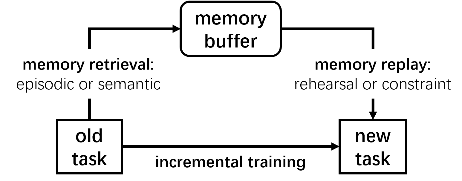
Figure 1: A generic framework of replay-based approaches.

Replay-based methods maintain a memory buffer preserving the information of prior tasks and replay it when learning new tasks to mitigate CF. As Figure 1 illustrates, in terms of memory retrieval, some methods extract episodic memory referring to specific experience (e.g., a subset of raw samples), whereas others extract semantic memory referring to some structural knowledge (e.g., generative pseudo samples, gradients over old tasks). Regarding memory replay, some approaches train the memory buffer with new data jointly, while others leverage the memory buffer to impose constraints on parameter updates in a similar manner to regularization-based methods. Hence, according to the ways of memory retrieval and replay, there are four sub-categories in replay-based methods: episodic and rehearsal (Isele and Cosgun (2018), Rolnick et al. (2019), de Masson d'Autume et al. (2019)), episodic and constraint (Rebuffi et al. (2017), Lopez-Paz and Ranzato (2017), Aljundi et al. (2019)), semantic and rehearsal (Farajtabar et al. (2020), Shin et al. (2017), Ostapenko et al. (2019)) and semantic and constraint.

Architecture-based approaches isolate parameters for each task to avoid CF and tackle the ‘concept drift’ problem. Some of them expand a branch of parameters for new tasks, while others select a task-specific subset of relevant parameters from parent networks (Rusu et al. (2016), Fernando et al. (2017), Serra et al. (2018)).

2.2 Dynamic Graph Learning

2.2.1 Graph statement

A static graph, defined as $\mathcal{G}=(V,E)$, contains a node (vertex) set $V$ and an edge set $E\subseteq V^{2}$. $\mathcal{G}$ is usually accompanied by some matrices describing the graph information from different aspects. An adjacent matrix $A\in R^{|V|\times|V|}$ models the topological structure of the graph, where $A_{ij}\in R_{+}$ if edge $(v_{i},v_{j})\in E$ and $A_{ij}=0$ if no connection exist between $v_{i}$ and $v_{j}$. A degree matrix $D\in R^{|V|\times|V|}$ is a diagonal matrix recording the degree of each node where $D_{ii}=\sum^{|V|}_{j=1}A_{ij}$.

According to (Xue et al. (2022)), dynamic graphs can be categorized as discrete and continuous. Discrete graphs can be decomposed as multiple snapshots $\{\mathcal{G}^{t}\}^{T}_{t=1}$ over a period of time, where each snapshot $\mathcal{G}^{t}=(V^{t},E^{t})$ is a static graph at the $t$-th time step. The snapshot at each time step evolved from its previous step as $\mathcal{G}^{t}=\mathcal{G}^{t-1}+\Delta G^{t}$. The update item $\Delta G^{t}$ includes a feature or topological update. Feature update can be the update of the feature values, the expansion or shrink of feature dimension or channel. The topological update can be node addition or deletion, edge addition or deletion. Continuous graphs evolve in a streaming manner. Usually, each graph component is annotated with a timestamp marking its birth time.

2.2.2 Dynamic graph learning techniques

Preserving spatial and temporal information is the fundamental challenge for DGL. Spatial information refers to knowledge about graph structure (e.g., neighbor interaction, node proximity) and temporal information refers to patterns of graph evolution (e.g., the interaction between nodes over different timestamps). Most DGL models contain two components: a spatial module for learning spatial patterns and a temporal module for capturing temporal patterns. TGCN (Zhao et al. (2020)), STGCN (Yu et al. (2018)) and DySAT (Sankar et al. (2020)) all employ GNNs to capture spatial features for each snapshot but they differ in their way of learning temporal patterns. TGCN adopts RNN, STGCN uses a temporal convolution layer and DySAT employs a self-attention mechanism. Some works incorporate the two components into one module. EvolveGCN (Pareja et al. (2020)) uses GNN to learn structure-aware node representation for each snapshot, but instead of feeding the snapshots to the temporal module, it employs RNN to train the weights of GNN to integrate structural information. GC-LSTM (Chen et al. (2022)) embeds GNN into long short-term memory (LSTM) cells to obtain the gate and hidden state. HAD-GNN (Tian et al. (2022)) employs an attentive LSTM network to encode temporal information and uses a graph attention network (Veličković et al. (2018)) to capture spatial knowledge.

The above methods feed the whole previous snapshot into the model, having the network decide what to preserve and abandon, which is costly and time-consuming. Some DGL works try to learn the evolution patterns incrementally. DANE (Li et al. (2017)) regards graph embedding as an eigen problem. DANE can incrementally update node embeddings based on matrix perturbation theory instead of re-computing the eigenvectors when the graph evolves. DyHNE (Wang et al. (2022d)) extends DANE to heterogeneous graphs and can also update node embeddings incrementally.

2.2.3 Relation with continual graph learning

DGL and CGL both aim to accommodate evolution patterns on dynamic graphs. Although they both preserve historical knowledge, their focuses are different. DGL merely focuses on knowledge forward transfer (i.e., how to leverage historical knowledge to support future learning); thus it tends to abandon out-of-date information. However, CGL also cares about knowledge backward transfer (i.e., how to utilize new knowledge to support previous tasks and how to prevent learned knowledge from ruining its previous knowledge). Large negative backward transfer causes catastrophic forgetting. Therefore, in CGL, even if some patterns are obsolete to the latest task, the model would not abandon them if they are significant to previous tasks.

3 Continual Graph Learning

3.1 Problem Statement

We introduce three typical GL tasks: node classification (NC), graph classification (GC) and link prediction (LP).

NC: Given a graph $\mathcal{G}=(V,E)$ where some nodes $v_{i}\in V$ associated with a label $y_{i}\in Y$. The objective is to figure out $p(y|v)$ by fitting the training set $p(Y_{train}|\mathcal{G}_{train})$. The unannotated nodes in $\mathcal{G}$ form the testing set $\mathcal{G}_{test}$. In the transductive setting, the testing subgraph is seen during training, implying $\mathcal{G}_{train}=\mathcal{G}$; in the inductive setting, the testing subgraph is inaccessible during training, where $\mathcal{G}_{train}=\mathcal{G}\backslash\mathcal{G}_{test}$.

GC: Given a training graph set $S^{\mathcal{G}}_{train}=\{\mathcal{G}_{1},\mathcal{G}_{2},...,\mathcal{G}_{n}\}$, each graph $\mathcal{G}_{i}$is associate with a label $y_{i}$. For each testing graph $\mathcal{G}_{test}\notin S^{\mathcal{G}}_{train}$, the objective is to figure out $p(y|\mathcal{G}_{test})$.

LP: Given a training graph $\mathcal{G}=(V,E\backslash E^{\prime})$, each edge $e\in E\backslash E^{\prime}$ is associated with a label $1$ denoting its existence in the graph. $E^{\prime}$ is an edge set whose edges are in graph $\mathcal{G}$ but invisible in the training process. The testing set is a set of edges $E_{test}$. Usually, $E_{test}$ covers $E^{\prime}$ and contains some fake edges. For each edge $e\in E_{test}$, the objective is to deduce whether $e$ exists in the original graph.

3.2 Novel Challenges

(a) CL setup: Samples with c.d assumption

(b) CGL setup: Samples without c.d assumption

Figure 2: Sample-level setup of CL and CGL. c.d denotes conditional independence; m.p denotes message passing.

(a) CL setup: Datasets with c.d assumption

(b) CGL setup: Datasets without c.d assumption

Figure 3: Dataset-level setup of CL and CGL.

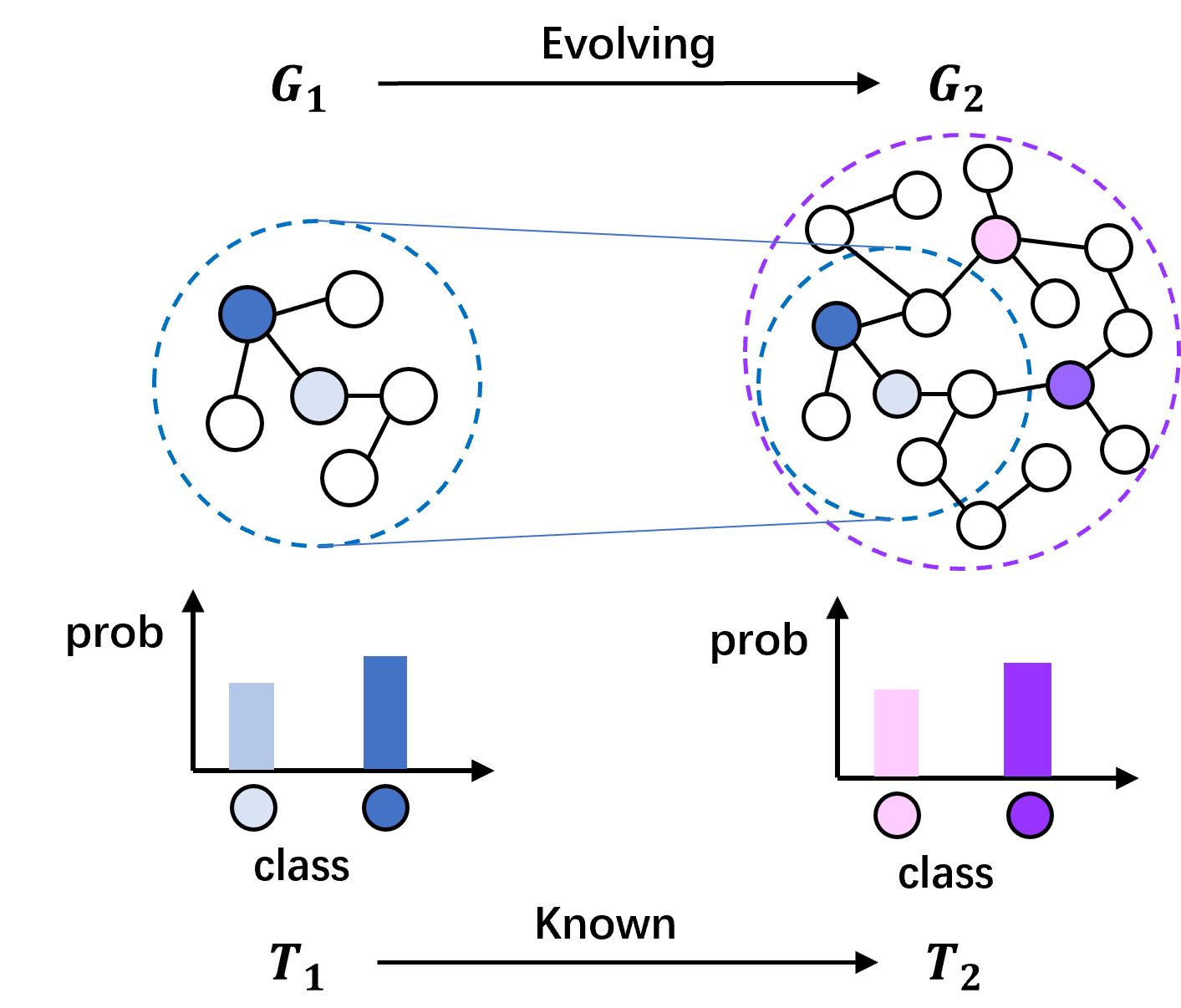
(a) Task-incremental

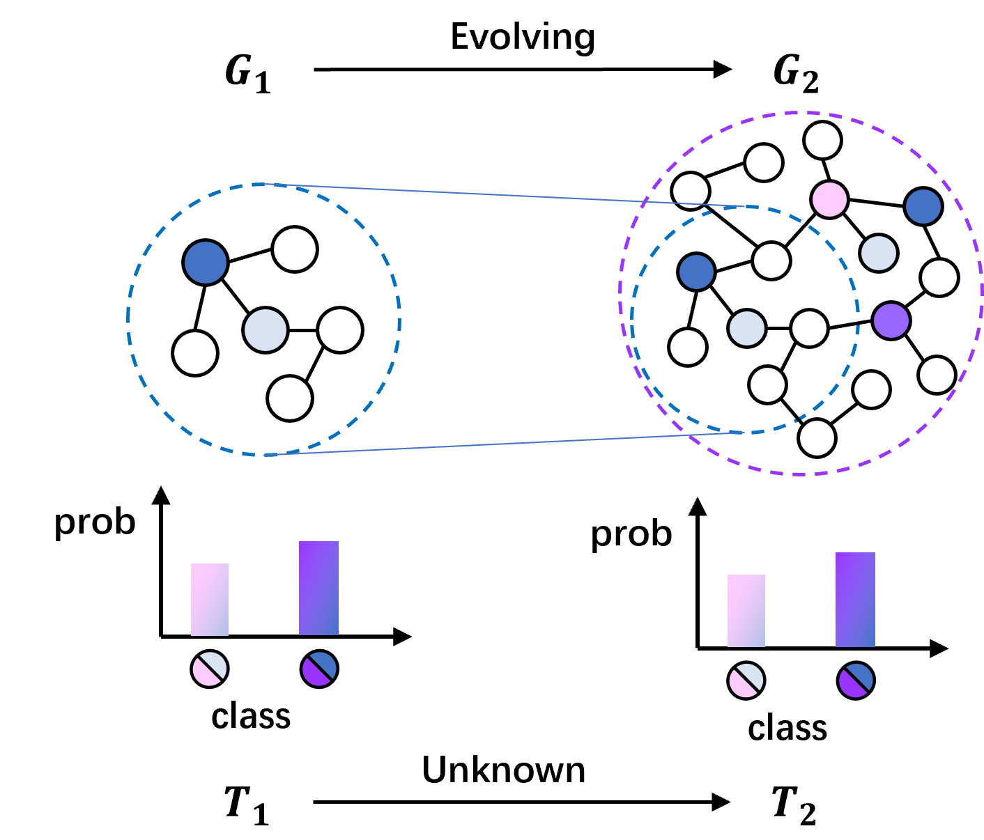
(b) Domain-incremental

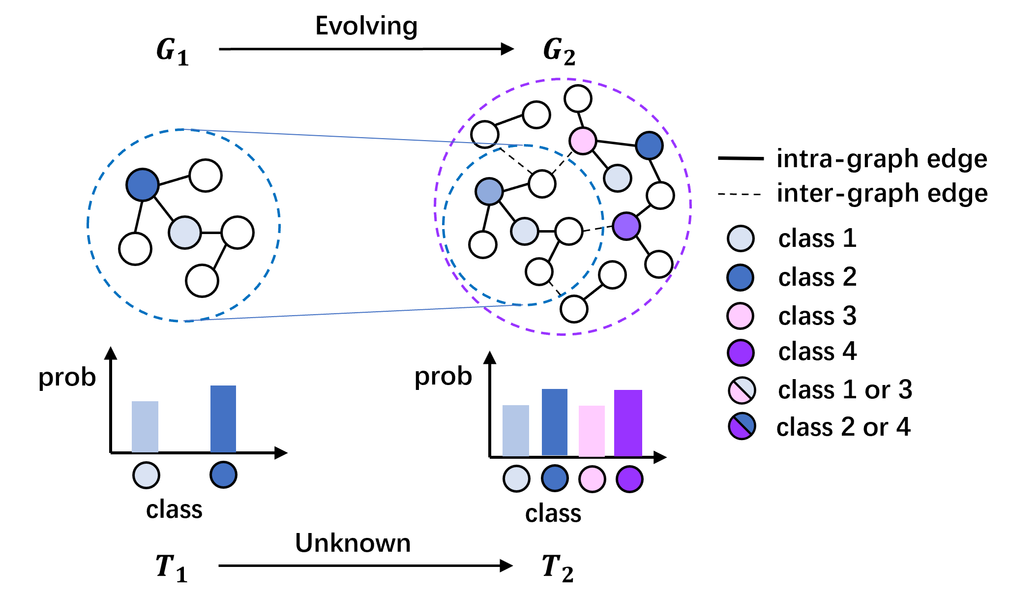
(c) Class-incremental

Figure 4: Three scenarios of CGL.

The graph-structured data import the sample-level dependency and graph-level dependency into CGL. Figure 3 describes the setup of CL and CGL from a sample-level view. In the CL setup, the samples are conditionally independent of each other, i.e., given $\theta$, $x_{1}$ provides no information for $x_{2}$. Hence, $x_{1}$ and $x_{3}$ do not involve the inference of $y_{2}$ and $\theta$ merely absorbs the feature information of samples. In the setup of CGL, due to the intra-graph edges between nodes, $x_{2}$ gains information from its neighbors $x_{1}$ and $x_{3}$. Therefore, even if $\theta$ has been figured out to deduce $y_{2}$, the information from $x_{1}$ and $x_{3}$ still makes a difference. $\theta$ absorbs the feature information and the structural information.

Graph (dataset)-level dependency refers to the dependency between the old dataset and the new incoming dataset in CGL. We illustrate the setup difference between CL and CGL from the dataset level based on the probabilistic graphical model shown in Figure 2. In the CL setup, the network parameters $\theta$ absorb all the information of previous tasks and are expected to fit the new task $D^{T}$. $\theta$ blocks the path from previous tasks $D^{1:T}$ to the current task $D^{T}$. Hence, observing $\theta$, we have $D^{1:T-1}\perp\!\!\!\perp D^{T}|\theta$. In the CGL setup, due to the inter-graph links between $D^{1:T-1}$ and $D^{T}$, their relationship cannot be entirely disentangled by $\theta$. Therefore, in CGL, we have the following:

$$p(\theta|D^{1:T})\propto p(\theta|D^{1:T-1})p(D^{T}|D^{1:T-1},\theta)$$ (2)

where the dependency between datasets is incorporated into $p(D^{T}|D^{1:T-1},\theta)$. Same as CL, the availability of $D^{1:T-1}$ is restricted, calling for efficient strategies to approximate the old patterns and the dependency.

3.3 Three Scenarios

Figure 4 demonstrates the three learning scenarios in CGL. In the task-IL scenario, the task descriptor is given, and the network is aware of the task update, indicating that the output neurons for each task are pre-defined. Also, the output space of each task is different. In the figure, task 1 predicts classes 1 and 2, whereas task 2 predicts classes 2 and 4. In the domain-IL scenario, the task descriptor is unavailable. The output spaces of all the tasks are consistent, indicating that the output neurons are shared among all tasks. Thereby in the figure, two output neurons take over two tasks. The first neuron outputs the possibility that a node belongs to class 1 or 3, and the second neuron is associative with class 2 or 4. The input distributions of these tasks are different. In task 1, the graph merely contains nodes from classes 1 and 2; In task 2, nodes from classes 3 and 4 appear. In the class-IL scenario, the task descriptor is invisible and the output spaces are different. The model has to accommodate different input distributions and identify samples from novel classes itself. As the figure shows, in task 1, the model is expected to predict classes 1 and 2; In task 2, with new classes coming, the model is expected to classify all observed categories.

3.4 Evaluation Metrics

Similar to CL, the performance of a well-trained model after observing $T$ task is evaluated in terms of four criteria: average performance (OP), forward transfer (FT), average forgetting (AF), and Intransigence (INT). Following (Lopez-Paz and Ranzato (2017)), we define the performance on task $i$ after visiting $j$ tasks as $P_{i,j}$ and define the performance on task $i$ with randomly initialized parameter as $R_{i}$. AP evaluates the network’s overall performance among all the tasks. FT aims to assess the model’s ability to leverage learned knowledge to support future learning. Specifically, it checks the performance improvement on task $i$ after the model acquires the knowledge of task $i-1$. AF evaluates the model’s capability of overcoming CF. It computes the performance deterioration of each task after the model observes later tasks. INT Chaudhry et al. (2019) measures the difference between the performances of joint training and the CL model after learning $T$ tasks. These metrics can be formulated as follows:

$$AP=\frac{\sum^{T}_{i=1}P_{i,T}}{T},FT=\frac{\sum^{T}_{i=2}P_{i,i-1}-R_{i}}{T-1},AF=\frac{\sum^{T-1}_{i=1}P_{i,T}-P_{i,i}}{T-1},INT=\frac{\sum^{T}_{i=1}P^{joint}_{i,i}-P_{i,i}}{T}$$

where $P^{joint}_{i,i}$ denotes the performance of a joint training model on task $i$ after learning $i$ tasks.

3.5 Approaches

In this section, we review the current CGL approaches following the taxonomy in Section 2.1.3.

3.5.1 Regularization-based

1) Weight-based: TWP (Liu et al. (2021)) employs a minimized loss preserving module similar to SI (Zenke et al. (2017)), which evaluates the parameter importance in terms of its contribution to the loss. The importance score of a parameter is quantified as its gradient magnitude of the loss function. Furthermore, TWP proposes a topological structure-preserving module aiming to maintain the dependency of each node with its neighbors. The total structural information of a graph at the $l$-th layer is represented as the squared L2 norm of edges weights. Then the gradient magnitude of this function can measure the parameter importance to topological information. The final importance score is formulated as a weighted sum of its loss-based importance and topological-based importance. Aside from GAT (Veličković et al. (2018)), the topological-aware module can extend to general GNNs. The work (Jha et al. (2021)) does not employ GNNs. It instead leverages an autoencoder to learn the node representation by reconstructing the network’s topological information, including local neighbor interaction, global node interaction, and biclique information. Therefore, the topological information is explicitly encoded into the loss function. This work then employs a weight-based regularization strategy to retain loss-sensitive and topology-sensitive parameters.

2) Distillation-based: GraphSAIL (Xu et al. (2020b)) introduces knowledge distillation into CGL on recommendation tasks. The dataset is a bipartite user-item graph, where an edge models the user’s preference for an item. GraphSAIL aims to retain both local and global structural information. For local structural information, it preserves the dot product between two node embeddings of each node with its neighbors. It preserves a node’s position in the whole graph for global structural information. To relieve the computation burden, it employs $K$-means algorithm to obtain $K$ clusters and maintains the similarity distribution of each node to these clusters. Furthermore, GraphSAIL imposes adjustable constraints on the update node embeddings. Updates of nodes with little proportion of new neighbors would be suppressed. The work (Wang et al. (2021b)) distills neighbor similarity among all layers to transfer knowledge from different receptive fields. Besides, this work adopts a contrastive distillation objective to prevent the student model from mapping different nodes to close representations. The two works require storing previous node embeddings, leading to high space complexity. The work (Ding et al. (2022)) proposes two novel modules: incremental graph convolution and colliding effect distillation, to fulfill CL in collaborative recommendation tasks. The former module performs neighbor aggregation on the incremental graph part and updates representations of active nodes (nodes connecting with new nodes) as a weighted sum of previous and new representations. The latter module updates the inactive nodes by injecting the representations of their $K$-nearest activate nodes into them, based on the assumption that node similarity/distance keeps stable. This could prevent patterns in inactive nodes from getting obsolete. This work requires storing the degree of each old node. The work Sun et al. (2022) is the first to explore self-supervised CGL. It argues existing approaches merely focus on Euclidean space (zero-curvature Riemannian space), neglecting the fact that curvature may vary over incoming graph sequences. Also, existing methods train the models under supervised scenarios, which are not piratical in a continually evolving graph. Due to the invisibility of curvature of incoming graphs, this work firstly proposes a unified GCN of arbitrary curvature, whose curvature is adaptively learned for each task by a novel neural module. While aiming to overcome CF, the label-free Lorentz distillation approach is proposed, which contains intra-distillation and inter-distillation. Distillation is performed in Riemannian space. Since curvature and feature dimension may vary among graphs, leading to Riemannian spaces with different curvature and dimensions, a novel Generalized Lorentz Projection is presented to map between different Reimannians spaces. After projection, intra-distillation controls the divergence between low-level and high-level node encoding, while inter-distillation evaluates the agreement of high-level node encoding between the teacher and student models.

3.5.2 Replay-based

1) Episodic and rehearsal: ContinualGNN (Wang et al. (2020)) designs replay strategies from two aspects: novel pattern detection and old pattern preservation. In terms of novel pattern detection, it samples a subset of old nodes that are easily perturbed by newly coming nodes (referred to as ‘perturbation propagation’). The perturbation of a node $i$ is quantified as its representation change after new data incomes. The nodes whose received perturbation exceeds the threshold are supposed to produce new patterns. In terms of old pattern preservation, the model employs hierarchical sampling strategies and importance-based sampling strategies to produce the memory. The former guarantees the consistency of category distribution between the memory and the entire dataset. The latter select nodes hold a large proportion of neighbors from other categories. These nodes are located at the class boundary and are supposed to contribute more to the gradient. Both two sampling methods are embedded into the reservoir sampling algorithm to accommodate the data stream. EWC regularization is also employed on the memory to mitigate memory overfitting. ContinualGNN mainly performs the experiments upon GraphSAGE with the mean aggregator. Being extended to other GNNs, the novel patterns detection module needs to be modified accordingly.

ER-GNN (Zhou and Cao (2021)) employs three replay-based strategies: Mean of Feature (MF), Coverage Maximization (CM) and Influence Maximization (IM). Drawing inspiration from iCaRL (Rebuffi et al. (2017)), MF treats the mean embedding of each category as its representative prototype and selects a subset of nodes closest to the prototype. The sampled nodes are expected to describe the core features of each category. Inspired by (de Bruin et al. (2016)), CM aims to maximize the embedding space coverage of nodes in the memory by selecting nodes far from the embedding space of other categories, which amounts to obtaining a uniform distribution of the training set. The nodes in the memory are expected to describe the general features of the whole dataset. IM aims to maximize the influence of nodes in the memory on the loss function. A node’s influence is quantified as the parameter change after removing it, which can be further transformed as the parameter change after upweighting the node slightly, based on the idea of influence function (Hampel et al. (2011), Koh and Liang (2017)). The method will select a fixed number of nodes with the largest influence in each category as the memory. However, the influence function is initially designed for i.i.d data (Hampel et al. (2011)). In graph-structured data, empirically, neighbors of an influential node are also likely to be influential. Taking sample-level dependency into the sampling strategy may be a potential research direction.

The work (Perini et al. (2022)) argues that challenging samples should be assigned higher priority to be rehearsed since they preserve the decision boundary. This work proposes a priority-based node sampling strategy based on the argument, selecting samples with higher losses.

The work (Ahrabian et al. (2021)) employs an inverse degree experience sampling strategy dedicated to recommendation tasks, where the data come from user-item interaction. Therefore, rather than node selecting, it selects a subset of interaction. This node strategy is proposed to suppress the sampling probability of interactions whose users have higher degrees (interact frequently), thereby encouraging the model to pay more attention to those with infrequent interactions. It is also embedded in reservoir sampling for continual sampling.

The work (Galke et al. (2021)) and IGCN (Xia et al. (2021b)) both employ temporal experience replay. The work (Galke et al. (2021)) leverages the time difference distribution regardless of time granularity to determine the history (memory) size. The occurrence times of the time difference (TD) $d$ on a node equals the number of neighbors that appear $d$ time steps earlier. Then the occurrence times of the TD $d$ on the entire graph can be obtained as the sum of TD $d$ over nodes. Given a graph $\mathcal{G}$ with $t$ times steps, i.e., $t$ previous tasks, the TD frequency with respect to $d$ on the graph can be firstly computed as:

$$td(d)=card(\{(u,v)|v\in\mathcal{G}\land u\in N(v)\land t(u)\leq t(v)\})$$ (3)

where $card()$ returns the element number of the set, $t()$ returns the time of the node and $N(v)$ denotes the neighbors of node $v$. Then the TD distribution with respect to $d$ can be easily acquired, and the history size can be selected to cover a certain proportion of the time differences. IGCN focuses on collaborative filtering tasks. The data, similar to that in GraphSAIL and GraphSAIL⁺, record the user-item interaction and can be constructed as heterogeneous graphs, with users and items as nodes and interactions as edges. The nodes are merely indexed without initial embeddings. IGCN stores $k$ steps historical data when performing tasks $t$. Given the newly observed data $D^{t}$, IGCN firstly employs the model agnostic meta-learning (MAML) (Finn et al. (2017)), a training paradigm that can equip the model with good generalization ability with limited training samples, to initialize the node embeddings of the data from task $t-d$ to $t$. After initialization, the data (subgraph) of recent $d$ task are fed into a GCN layer, producing $d$ enriched topological aware node representation matrix. Subsequently, a modified TCN network (Bai et al. (2018)), called iTCN, is used to map the $d$ node representation matrices to a fused one, which is expected to capture the evolving temporal features of users and items. Finally, the interaction between a user and an item can be obtained as the dot product of their embeddings.

The two works assume that the previously learned patterns gradually become obsolete over time and merely focus on short-time patterns. However, long-time patterns that stay stable overall time are ignored.

TrafficStream (Chen et al. (2021)) explores CGL on traffic flow prediction tasks. The traffic network is more complicated than the dynamic graphs in other CGL methods since both node attributes and the graph topology change over time. The node in the traffic network usually denotes a sensor deployed on the roads and the node attribute is the traffic flow recorded by the sensor within a period (Ye et al. (2020)). To retain old flow patterns, TrafficStream samples a set of nodes with a stable flow as the episodic memory and rehearses their flow in the future. Besides, an EWC regularization is also imposed on the network parameters. To tackle the graph-level dependency, it selects the neighbors of the newly evolved subgraph as the memory to replay. The work (Tan et al. (2022)) explores CGL in few-shot scenarios where the labeled data of new classes are sparse. With new classes incoming, it forms a novel support set and a novel query set that is sampled from new data. The two sets are then merged into the previous support sets and query sets, respectively. Incremental meta-learning is performed upon the two merged sets. Furthermore, to tackle the class-imbalance challenge, this work proposes a hierarchical attention mechanism, including task and node levels. Task-level attention aims to adjust the weight of loss on each task according to its importance. The task importance is obtained from a task prototype computed as a weighted sum of node features. Node-level attention aims to compute the weight of each node in generating the task prototype.

2) Semantic and constraints: HPN (Zhang et al. (2022a)) leverages hierarchical graph representation to realize stability and plasticity simultaneously. It disentangles each node embedding into a set of atomic embeddings, maintaining feature-based information and a set of structural embeddings denoting topological information. They are respectively generated by performing a series of linear transformations upon the node’s initial embedding and a sampled set of the node’s neighbors. A divergence loss is adopted to guarantee the diversity of the generated embeddings. The atomic and structural embeddings of the first node are directly regarded as the atomic-level prototype $P_{A}$, which is expected to maintain the atomic-level features of the nodes (E.g., user gender and personality in the user-item interaction graph). The node-level prototype is produced by linearly transforming the concatenated atomic-level prototypes, which describe the general node information. The class-level prototype is generated by linearly transforming the concatenated node-level prototypes, which model the high-level features among similar nodes. Given a newly observed node $v$, HPN acquires its atomic embedding set and structural embedding set at first. Then it measures the cosine similarity between the extracted embeddings of $v$ and each atomic-level prototype in $P(A)$. For those similar embeddings and prototypes, a distance loss is imposed to narrow their gaps, thus retaining the learned; whereas those remaining extracted embeddings of $v$ that are not similar to any existing atomic-level prototype are thought to generate novel patterns and would be merged into the atomic-level prototypes. After updating $P(A)$, HPN computes the cosine similarity again and the matched prototypes $A(v)$ are regarded as the novel atomic embedding of node $v$. Then its node-level embedding is produced based on $A(v)$. Node $v$ obtains a novel node-level embedding $N(v)$ similarity and vice verse acquires the novel class-level embedding $C(v)$. The network outputs the category of $v$ via an MLP on the concatenated three-level embeddings.

The work (Han et al. (2020)) belongs to the subcategory of episodic and constraints, which simply applies GEM and EWC without a CGL-specific setting.

SGNN-GR (Wang et al. (2022b)) belongs to the subcategory of semantic and rehearsal. It argues existing episodic and rehearsal methods fail to preserve previous knowledge fully due to their limited memory buffers. To maintain complete data distribution, SGNN-GR injects historical knowledge into a generative model (GM) and has the generator to produce pseudo samples. Since GNN is the base GL model, which merely observes the receptive field of each node, to benefit GNN training on the memory, the GM learns to generate neighborhoods for fake nodes. The training data of GM are random walks with restart (RWR) on the previous graph. Training with RWRs is more likely to preserve complete previous knowledge since it is theoretically shown that RWRs can quickly transverse the neighbors. Furthermore, SGNN-GR identifies changed nodes and stable nodes. The changed nodes include new nodes and previous nodes that are greatly perturbed. The GM and GNN are then trained incrementally with changed nodes. Besides, a filtering strategy is proposed to filter the nodes sharing similar patterns with the previous patterns of affected nodes in the training set of GM. This could prevent GM from generating disappearing patterns.

3.5.3 Architecture-based

DiCGRL (Kou et al. (2020)) inspects knowledge graph completion and node classification tasks. Based on the hypothesis that each node holds several independent semantic aspects, DiCGRL decomposes node embedding into several components respecting different semantic aspects, respectively. In a knowledge graph, when training a triplet $(v_{i},e_{ij},v_{j})$, $v_{i}$ and $v_{j}$ merely update their semantic components relevant to the relation $e_{ij}$. In a node classification task without explicit relation, a node merely updates its semantic component that is relevant to its connected nodes. The relevance can be quantified as the attention score; only the semantic components with the top-n highest attention scores would update. To accommodate new patterns, DiCGRL also employs a neighbor activation replay-based strategy, which selects the 1-hop and 2-hop neighbors of the new graph from the previous graphs as the episodic memory to rehearse. However, it lacks attention to refining the learned knowledge in the inactivated part of the old graph.

MSCGL (Cai et al. (2022)) lies in the intersection between architecture-based and regularization-based approaches. Drawing inspiration from GraphNAS (Gao et al. (2019)), it trains a controller with reinforcement learning to search for the optimal architecture for each task. The search space contains a list of components of GNNs, including aggregation, activation, and correlation evaluation operations. The parameters are shared between the same aggregations among the tasks to reduce unnecessary model expansion. Furthermore, MSCGL imposes sparse group constraints on all parameters and imposes an orthogonal constraint on the shared parameters. The former retains critical knowledge of the previous tasks and the latter prevents the parameter update from interfering with previous performance.

FGN (Wang et al. (2022a)) transforms the graph-structured data into independent data with the feature map. Thus the traditional CL strategies can be naturally applied to the CGL problems. The feature map implicitly encoders the sample-level dependency into the feature-level relationship, converting an original node classification task into a feature graph classification task. After that, FGN employs GSS (Aljundi et al. (2019)) to support CL. This method is a trade-off between the utilization of topological information and the compatibility with conventional CL approaches.

3.6 Public Datasets

We summarize some benchmark datasets of continual graph learning in Table 2. Note that the datasets with static graphs can be adapted to the dynamic GL task with other splitting methods (Wang et al. (2020)). Datasets for node classification tasks include Cora (Sen et al. (2008)), Citeseer (Sen et al. (2008)), PPI (Zitnik and Leskovec (2017)), Corafull (Bojchevski and Günnemann (2017)), Amazon Computer, Reddit (Hamilton et al. (2017)), Elliptic, and DBLP-sub (Tang et al. (2008)). Datasets for link prediction tasks include FB15k-237 (Toutanova and Chen (2015)) and WN18RR (Dettmers et al. (2018)). Datasets for graph classification tasks include ogbg-molhiv (Wu et al. (2018)) and Tox21 (Huang et al. (2014)).

Table 2: Summary of public datasets. G is graph number, v is vertex number, E is edge number, C is class number, NF is feature dimension, EF is edge feature dimension, T is a triple number, RT is relation type, S is the snapshot number of a dynamic graph, and each snapshot is the data of a task.

Task	Dataset	G	V	E	C	NF/EF	S	Description
NC	Cora	1	2,708	5,492	7	1,433/0	-	citation
	Citeseer	1	3,327	9,104	6	3,703/0	-	citation
	PPI	24	2,372(Avg)	34,113.2(Avg)	121	50/0	-	protein-protein interaction
	Corafull	1	19,793	65,311	70	8,710/0	-	citation
	Amazon Computer	1	13,752	245,778	10	767/0	-	co-purchase
	Reddit	1	232,965	11,606,919	50	602/0	-	post-to-post
	Elliptic	1	203,769	234,355	2	166/0	9	transaction
	DBLP-sub	1	20,000	75,706	9	128/0	14	citation
Task	Dataset	G	V	T	RT	NF/EF	S	Description
LP	FB15K-237	1	14,541	310,116	237	0/0	-	knowledge graph
	WN18RR	1	40,943	151,442	18	0/0	-	word net
Task	Dataset	G	V(Avg)	E(Avg)	C	NF/EF	S	Description
GC	ogbg-molhiv	41,127	25.5	27.5	2	9/3	-	molecule
	Tox21	7,831	18.6	-	12	801/0		molecule

3.7 Discussion

3.7.1 Sample-level and graph-level dependency

The two dependencies are brought from graph topology, differing CGL from CGL, and thus should be considered in the first place. The following questions should be answered: 1) What is a sample-level dependency? 2) Why is maintaining sample-level dependency essential? 3) What is a graph-level dependency? 4) Why is capturing graph-level dependency essential?

1) Sample-level dependency comes from inner task links and covers a list of structure properties, including betweenness, distance distribution, clustering, etc. (Mahadevan et al. (2006)). Besides, it can be some post-defined features such as node co-occurrence and neighbor interaction.

2) Most GL models are unaware of their learned topological knowledge, i.e., structural features are learned implicitly (Bouritsas et al. (2022), Horn et al. (2021)). In GNNs, edge weights are indifferent to the loss function and other structural properties do not involve aggregation. Therefore, the network mainly focuses on output performance regardless of its learned structural information quality. Since many parameter distributions would lead to a similar performance (Hecht-Nielsen (1992), Sussmann (1992)), some parameter configurations might achieve good performance but with poor structural representation. Hence, preserving loss-based knowledge cannot guarantee proper structural representation. Thus it is necessary to guide the model to retain structural representation.

Retaining previous topological features can enhance the network’s generalization ability among tasks. (Yim et al. (2017)) interprets the network’s output as the answer to a question, the middle layer as the intermediate results, and the relation between features as the solution. Topological information can be regarded as a kind of solution. The network that merely remembers the results is vulnerable to task updates, while the network that remembers the solutions is more robust and can adapt to a list of similar tasks. Furthermore, in CGL tasks, a new graph evolves from its previous graph, inheriting its topological information. Hence it is reasonable to retain structural representation.

3) Graph-level dependency refers to the mutual influence between the novel and old graphs. It can be explicit information propagation or other implicit interactions.

4) Capturing graph-level dependency mainly serves for learning novel patterns. On the one hand, the influence of the old graph could help learn novel patterns in the evolved graph. On the other hand, the influence of the novel graph might bring new patterns to the old graph or even eliminate previously learned patterns.

3.7.2 Regularization-based approaches

Regularization-based approaches excel at maintaining sample-level dependency but might encounter difficulty in retaining graph-level dependency.

The major concerns of regularization-based approaches are: 1) Which kind of topological information is crucial to the task? 2) How to encode structural information? First, the importance of topological information depends on the GL models, graph properties and tasks. Different GL models focus on different topological information. It is natural to maintain learned structural information of GL models. For instance, employing GAT, TWP defines the loss function based on the sum of the edge weights. Second, regarding the encoding method of the structural information, effectiveness, flexibility and efficiency should be well evaluated. TWP offers an elegant encoding, which requires a slight computation burden and can be adapted to most GL models. However, the distillation strategy of GraphSAIL is computationally expensive and non-data-free (requires much information from previous data). In traditional CL tasks, there exist many data-free distillation-based approaches. Also, the works in (Chen et al. (2020), Deng and Zhang (2021)) study data-free distillation for gnns, which might provide some insights into the potential improvements.

The limitation of regularization-based approaches lies in their weakness in addressing graph-level dependency due to the inaccessibility of previous data. Although a new task can implicitly recall previous knowledge, the new subgraph’s perturbation to the previous one is overlooked.

3.7.3 Replay-based

In CGL, the replay-based approaches can be mainly classified as episodic & rehearsal semantic & constraints, and semantic & rehearsal. Node selection strategies are arguably the core of the episodic and rehearsal methods, which can be designed for two objectives. First, similar to conventional CL, representative nodes of the previous task are selected as the experience to be rehearsed in the future to help circumvent CF. Second, in CGL, graph-level dependency might lead to new patterns emerging on the previous graph and perturb existing patterns. Therefore, nodes that might receive high perturbation also need rehearsal to accommodate novel patterns.

In terms of the first objective, the question is: How to measure the node importance for a task? We have introduced some node selection strategies, such as the mean of feature and coverage maximization. However, these node-sampling strategies are designed for i.i.d data. It is essential to propose node selection strategies to maintain representative topological information. There exists a number of measurements of node importance based on graph topology from a different perspective. Centrality is a typical measurement of a node’s position importance, including degree centrality, closeness centrality, betweenness centrality, eigenvector centrality, etc. (Kleinberg et al. (1999), Zhang and Luo (2017), Ruhnau (2000)). PageRank (Page et al. (1999)) and HITS (Kleinberg (1999)) are two heuristic algorithms assessing node importance based on link analysis. A drawback of these measurements is that they entirely depend on the raw graph topology, treating nodes evenly regardless of their contextual information. In attribute graphs, node embedding plays a pivotal role and should be carefully evaluated when designing node selection strategies. Weighted PageRank (Xing and Ghorbani (2004)) and weighted HITS (Zhang et al. (2007)) are two extensions of PageRank and HITS that integrate edge weights into node importance assessment. AttriRank (Hsu et al. (2017)) leverages random walk to integrate topological information and node attribute for importance measurement.

As for the second objective, i.e., to tackle graph-level dependency, a critical hypothesis is that a new subgraph perturbs only a tiny proportion of the old graph. In Section 3.1, we show the objective can be transformed as $p(\theta|\mathcal{G}^{t-1})p(\Delta\mathcal{G}^{t}|\mathcal{G}^{t-1},\theta)$. We can further decompose $\mathcal{G}^{t-1}$ as two subgraphs $\mathcal{G}^{t-1}_{p}$ and $\mathcal{G}^{t-1}_{np}$, where $\mathcal{G}^{t-1}_{p}$ is the subgraph perturbed by the new subgraph $\Delta\mathcal{G}^{t}$ and $\mathcal{G}^{t-1}_{np}$ is the subgraph that keeps stable regardless of the graph update. The probabilistic graph is shown in Figure 5, according to which we can obtain $p(\Delta\mathcal{G}^{t}|\mathcal{G}^{t-1}_{np},\mathcal{G}^{t-1}_{p},\theta)=p(\Delta\mathcal{G}^{t}|\mathcal{G}^{t-1}_{p},\theta)$. Therefore, the objective can be written as $p(\theta|\mathcal{G}^{t-1})p(\Delta\mathcal{G}^{t}|\mathcal{G}^{t-1}_{p},\theta)$, where $p(\theta|\mathcal{G}^{t-1})$ preserves the historical knowledge and $p(\Delta\mathcal{G}^{t}|\mathcal{G}^{t-1}_{p},\theta)$ prompts us to identify a subgraph that is susceptible to a new incoming subgraph, to help capture new patterns. We have introduced two node-sampling strategies for addressing graph-level dependency: perturbation propagation in ContinualGNN and neighbor activation in DiCGRL and TrafficStream. The former regards the node representation of novel nodes as perturbations and assumes the perturbation can propagate among the graph, similar to message passing; the latter is also based on the local neighbor aggregation mechanism of GNNs. Therefore, it simply samples the neighbors of the newly added nodes. Both strategies merely consider graph topology but ignore contextual interaction between node representation. Intuitively, even though an old node receives substantial information from the novel subgraph, its existing pattern can still stay stable if the received new information is consistent with the learned knowledge, and thus it needs no rehearsal.

Figure 5: Probabilistic graph model of rehearsal methods for tackling graph-level dependency.

Regarding the semantic and constraints methods, the way to distill high-level semantic knowledge undoubtedly deserves considerable attention. Two major questions should be considered: 1) How to encode the existing graph’s feature-level information and the sample-level dependency (topological information)? 2) How to accommodate new patterns to the extracted prior abstract patterns? HPN (Zhang et al. (2022a)) proposes a hierarchical representation of the continually evolving graph. To tackle graph-level dependency, it considers the mutual interaction between the novel patterns and the existing patterns. The newly learned patterns will strengthen the impression of existing knowledge if consistent with some existing patterns, otherwise will be added to the memory as novel knowledge. However, HPN is criticized for its cumbersome model design. Also, topological information is not efficiently utilized, which merely takes part in producing low-level prototypes via MLP. Graph pooling operation aims to learn hierarchical graph representation by producing informative subgraphs (Ying et al. (2018), Gao and Ji (2019), Lee et al. (2019), Yuan and Ji (2020), Gao et al. (2021), Zhang et al. (2019b)), which might provide some insights into extracting semantic knowledge in CGL. The works in (Yuan and Ji (2020), Gao et al. (2021), Zhang et al. (2019b)) explicitly encode topological information into the generated coarse graph.

In terms of the semantic and rehearsal methods, the core lies in strategies to generate fake samples and incrementally update the generative model (GM). In contrast with episodic replay, the advantages of generative replay are: 1) Generative models are trained with a large number of raw samples, thereby preserving richer historical knowledge; 2) Generative models can produce diverse fake samples, which better supports knowledge consolidation and avoids memory overfitting. 3) Generative replay partially resolves the concern of data privacy for avoiding producing raw samples; 4) Low space complexity: store the model instead of samples. The challenge of generative replay methods is to reach a balance between effectiveness and efficiency. Involving network training, normally, the time complexity of generative replay is higher than episodic memory. It is meaningless to employ generative replay if training a generative model costs more than retraining all previous data. To reduce time complexity, SGNN-GR (Wang et al. (2022b)) decides to adopt random walks with restart (RWR) instead of conventional random walks because, with a fixed number of training samples, RWR preserves more neighbor information. The time complexity is likely to be further reduced according to work (Rendsburg et al. (2020)) which argues that GAN is not a necessary ingredient in reproducing a large number of patterns. Effectiveness is related to the design of graph properties. The base GL models and graph properties should be considered (e.g., SGNN-GR tries to reconstruct neighbor information since it is friendly to GNNs). NetGAN (Bojchevski et al. (2018)) employs high-order (more than 2) random walks as the training set of GAN, aiming to preserve graph properties including network community structure and degree distribution, which is compatible with random-walk-based GL models (e.g., DeepWalk (Perozzi et al. (2014))). The work (Zhou et al. (2020)) is designed for temporal recommendation graphs, which can preserve structural and temporal patterns. A preprint work (Li et al. (2022)) designs a generative graph model for traffic networks, which can be extended to other spatio-temporal graphs.

3.7.4 Architecture-based

This family of methods alters network architecture to realize CL. Some works isolate network components for specific tasks or scenarios to mitigate CF (Kou et al. (2020), Cai et al. (2022)). Although component isolation might expand network size, it is necessary in cases where some tasks are dissimilar. Dissimilar tasks are likely to hold two utterly different solution regions. Therefore, performing all tasks with the same network can hardly achieve satisfactory performance on each task. Also, regularization-based strategies with elastic penalties, such as EWC assume that there is an intersection among the solution regions of tasks; thereby, they also fail to handle dissimilar tasks. However, isolating specific components for each task may degenerate CL into generic machine learning, i.e., training an independent network for each task, with high computation and memory overhead. Hence, component sharing is also essential for architecture-based approaches to realize knowledge transfer. Based on the above discussion, two questions should be considered when designing architecture-based approaches: 1) Under what conditions do we need to separate/share the network component? 2) How to mitigate CF when reusing shared components?

Regarding the first question, strategies to determine the conditions can be categorized as heuristic and non-heuristic. Heuristic strategies exploit prior empirical knowledge to make decisions. Some works assume each new task is unrelated to previous ones, allocating it to a specific network component (Rusu et al. (2016), Mallya et al. (2018)). Although effective, the network size increases linearly with tasks incoming in worst cases, leading to high computation and memory overhead. Intuitively, the components should be shared among similar tasks or scenarios to realize knowledge forward transfer and control space complexity. For dissimilar ones, the components should be isolated. Furthermore, network expansion is merely necessary if existing parameters cannot elegantly solve new tasks, otherwise is a waste of source. Heuristic strategies are scarcely investigated in CGL, but researchers can draw inspiration from CL works. The work (Yoon et al. (2018)) decomposes task similarity into unit-level. It measures the semantic drift of each hidden unit. Those with mild deviations are shared among tasks, whereas those with large deviations are duplicated for new tasks. Furthermore, DEN would grow branch networks for challenging new tasks (loss is above the threshold). The work (Sokar et al. (2021)) detects task similarity by measuring forward transfer. A new task is similar to previous ones if identifying a positive forward transfer. In CGL, considering that GL models exploit graph topology, graph similarity is a potentially critical factor for determining whether to isolate parameters. For instance, we can encode graph topology explicitly, such as TWP (Liu et al. (2021)) and measure the topology drift of each hidden unit. Those with high topology drift are likely to ruin the learned topological knowledge with new incoming tasks, and thus they should be isolated among tasks. Non-heuristic strategies encourage the network to learn component isolation. DiCGRL (Kou et al. (2020)) and MSCGL (Cai et al. (2022)) are two CGL projects with non-heuristic strategies. DiCGRL imports attention mechanism to select relative components and MSCGL employs reinforcement learning to search for optimal network architectures. Other strategies, such as trainable task-specific masks of parameters (Serra et al. (2018)), can be inspected in the future.

Regarding the second question, most CL strategies can be applied to the shared components to retain learned knowledge. E.g., MSCGL (Cai et al. (2022)) performs orthogonal learning and DEN (Yoon et al. (2018)) employs elastic penalty. However, current works merely focus on loss-based knowledge. Since TWP (Liu et al. (2021)) manifests the effectiveness of retaining topological knowledge, preserving learned graph topology in shared components may lead to improvement.

4 Open issues of CGL

We have investigated mainstream CGL approaches and provided a comprehensive discussion of CGL from a technical perspective. In this section, we summarize some open issues and challenges in CGL.

4.1 Graph robustness

GNNs suffer from vulnerability to adversarial perturbation on topology (e.g., edge add/delete) or node representation (e.g., feature modification), which limits GNNs’ application in safety-critical fields (Xu et al. (2020a), Jin et al. (2020)). This problem might be more severe in CGL. In order to relieve the computation overhead, generic CGL approaches compress the previously learned knowledge into a memory buffer (e.g., a parameter importance matrix, a set of informative nodes, or a representative subgraph). Tampering with the memory buffer can dramatically ruin knowledge consolidation for 1) the memory buffer is of small scale and thus is sensitive to perturbation; 2) The network’s awareness of the previous tasks is entirely based on the memory buffer. Therefore, the graph robustness in CGL deserves attention.

4.2 Compatibility of GL Models and beyond

Currently, CGL methods are highly dependent on GNNs. Hence, the way to distill topological information is highly related to the learned topological information of GL models. Given that there are numerous variants of GNNs employing different aggregation mechanisms and there exist other GL models except for GNNs such as DeepWalk, the compatibility of CGL strategy with various GL models needs to be evaluated. Furthermore, generic GNNs struggle to learn global structural information, encouraging CGL strategies to dig for other significant topological information to compensate for the limitation of GNNs.

4.3 Graph Multi-modality

Multi-modal graphs refer to those whose node features or edge features come from different domains (e.g., audio and text). A normal method to handle a multi-modal graph is to regard it as several independent single-modal graphs, perform GL upon each graph and finally combine the generated representation of each modality (Wei et al. (2019), Tao et al. (2020)). This is not challenging for CGL since CGL can perform CL strategies on each graph separately and fuse multi-modal information as well such as (Cai et al. (2022)). However, these methods merely consider the inner-modal interaction, while inter-modal relation also plays a pivotal role (Cheng et al. (2022)). CGL approaches for preserving inter-modal interplay on multi-modal graphs deserve future research.

4.4 Graph Heterogeneity

Heterogeneous graphs contain multiple nodes or edge types, requiring GL models to capture both graph topology and node feature heterogeneity. There are extensive works investigating static heterogeneous graphs (Chang et al. (2015), Shi et al. (2018), Chen et al. (2018), Zhang et al. (2019a)), which cannot adapt to dynamic graph evolution. There also exists a series of works exploring dynamic heterogeneous graphs (Wang et al. (2022e), Bian et al. (2019), Xue et al. (2021)). They can be roughly categorized as incremental and retrained approaches. The former merely preserves short-term memory without alleviating CF, while the latter is criticized for high computational costs (Wang et al. (2022c)). Besides, existing CGL on heterogeneous graphs merely explores the knowledge graphs and bipartite graphs. Studies of CGL on complex heterogeneous graphs with intricate meta paths are lacking.

5 Potential Applications of CGL

Existing works are mostly designed for simple scenarios (e.g., node classification for a small citation network).

5.1 Traffic prediction

Traffic networks are natural graph structures. Usually, edges denote roads and nodes are places where sensors are deployed. Sensors measure traffic states, including traffic volume, speed, or density (Nagy and Simon (2018)). According to Figure 6, there are four kinds of dependencies to note. The brown edges denote sample-level dependency, which exists between old nodes. It requires the model to retain topological knowledge (e.g., node interaction). The red edges represent the graph-level dependency that exists between the new graph and the old graph. It may lead to the emergence of new patterns on the old graph. E.g., some new roads are built; therefore, traveling routes may change accordingly. Furthermore, some learned patterns on the old graph may become obsolete. The blue arrows indicate the temporal dependency that models the correlation between a node and itself at the next time. Nodes with stable flow contain strong temporal dependency. The green edges indicate the spatial-temporal dependency that models the influence of a node on its neighbors at the next time step. Some nodes may be more dependent on others than on themselves. E.g., given two nodes $u$ and $v$ on the road and the vehicle travel from $u$ to $v$, the traffic flow of $v$ is highly related to that of $u$. Spatial-temporal dependency is prominent in traffic networks because it costs time for a vehicle to travel from one node to another. Therefore, the influence of a node on another is delayed.

There exists a CGL research on traffic prediction tasks (Chen et al. (2021)). It replays 2-hop neighbors of new graphs and nodes with unstable flows to accommodate new patterns and replays nodes with stable flows to consolidate old patterns and employs EWC regularization. Although achieving satisfactory performance, this work only evaluates some of the challenges in this task. First, this work neglects sample-level dependency and spatial-temporal dependency. While aiming to retain sample-level dependency, a feasible solution is to explicitly encode the node similarity and perform distillation or parameter smoothing. Following (Chen et al. (2021)), Jensen–Shannon divergence (JSD) can be imported to compute the node similarity. Temporal dependency may lead to similarity updates. Therefore, it is necessary to consider the stability of similarity since unstable stability may soon become obsolete and thus is insignificant to preserve. Intuitively, if two nodes are stable, their similarity is stable, either. Referring to (Chen et al. (2021)), given a previous graph $\mathcal{G}_{t-1}$ and a current graph $\mathcal{G}_{t}$, the stability of node $u$ can be computed as $JSD(P^{u}_{t-1}||P^{u}_{t})$, where $P^{u}_{t}$ denotes the distribution of representation of node $u$ at task $t$. Lower $JSD$ indicates higher stability. Hence, the importance of a node interaction $I_{e}$ can be written as:

$$I_{e}=\frac{SIM(u,v)}{S(u)S(v)}=\frac{JSD(P^{u}_{t}||P^{v}_{t})}{JSD(P^{u}_{t-1}||P^{u}_{t})JSD(P^{v}_{t-1}||P^{v}_{t})}$$ (4)

Where $SIM(u,v)$ represents the similarity of node $u$ and $v$, $S(u)$ denotes the stability of node $u$. The interaction importance is encoding of topological knowledge and can be utilized to guide the update of parameters (e.g., in a similar way as (Liu et al. (2021))).

Spatial-temporal dependency is prominent in traffic networks because it costs time for vehicles to travel from one node to another. Therefore, the influence of a node on another is delayed. It is reasonable to take the influence delay into account in computing node similarity. Concretely, suppose the distance between two nodes $u$ and $v$ is 1 mile which takes about 90 seconds for a car to cover on average, and the sensors record traffic flow every 30 seconds. Hence it takes three time-steps for the information of one node to reach the other. Also, suppose that we select five steps of flow data as node attributes, e.g., the attributes of node $u$ is $X^{u}=(x^{u}_{\tau},x^{u}_{\tau+1},...,x^{u}_{\tau+4})$ where $x^{u}_{\tau}$ denotes the traffic flow of node $u$ at time step $\tau$. If the vehicle travel from $u$ to $v$, the influence of $u$ on $v$ can be computed as $JSD(P(x^{u}_{\tau},x^{u}_{\tau+1},...,x^{u}_{\tau+4})||P(x^{v}_{\tau+3},x^{v}_{\tau+4},...,x^{v}_{\tau+7}))$ since it takes three time steps for the information on $u$ to reach $v$. To sum up, the time of information propagation deserves further research in traffic prediction tasks.

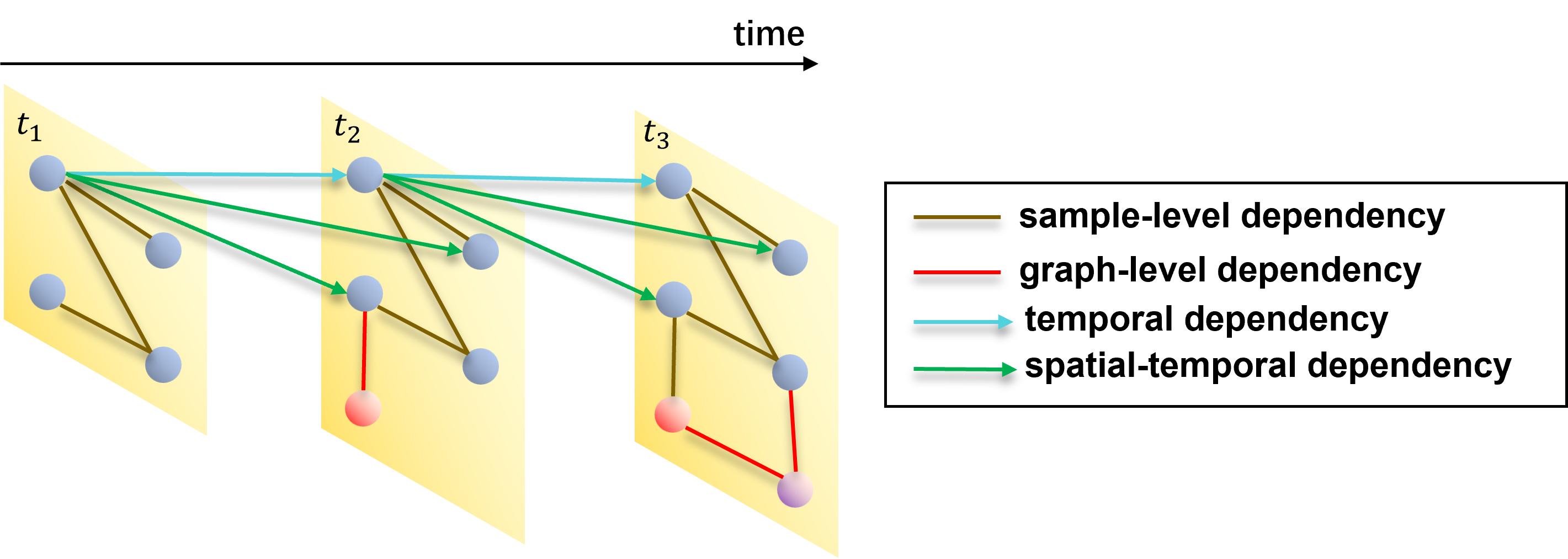
Figure 6: Illustration of meta-paths in heterogeneous graphs.

5.2 Finance

The intricate relations between various components in a complicated financial system make graphs a prevalent data structure representing complex relational data. According to work (Wang et al. (2021a)), components and relations in a financial system tend to evolve frequently and financial graphs are usually time-varying, which makes CGL a potential development direction in this field. However, graph and data properties in finance impose challenges in applying CGL to this field. Graph Heterogeneity is ubiquitous in finance, including account-device graphs, heterogeneous information networks, and financial knowledge graphs. Although some CGL works inspect heterogeneous graphs exist (Xu et al. (2020b), Ahrabian et al. (2021), Jha et al. (2021), Wang et al. (2021b), Ding et al. (2022)), they hardly explore interactions between nodes from different types. For instance, GraphSail performs distillation on node interactions and representations to retain information. However, the information of common interest among users is not well-modeled (two users prefer the same item). Meta-paths describe composite relations in heterogeneous graphs (Wang et al. (2022e)). Figure 7 illustrates a heterogeneous graph containing three types of nodes: user, item and manufacturer. There is no direct link connecting users, but user interactions can be modeled with meta-paths. The path $UIU$ identifies users with similar interests and the path $UIMIU$ finds users who prefer items from the same manufacturer. The node representations of users connected by meta-paths should be placed closely in the space. We can construct an adjacent matrix for each meta-path, modeling the interaction between nodes. In Figure 7, we provide adjacent matrices for path $UIU$ and $UIMIU$ among users, notated as $A^{UIU}$ and $A^{UIMIU}$, where $A^{p}_{ij}$ denotes the number of path $p$ connecting user $i$ and $j$. The adjacent matrices can be utilized for knowledge consolidation. For instance, we can add the adjacent matrices of all paths and normalize each element to $[0,1]$. Then we obtain a matrix $W$ where $W_{ij}$ indicates the importance of interaction between user $i$ and $j$. The interaction between user $i$ can $j$ can be obtained as their dot product or by performing linear transformation upon their representations. Then by multiplying each interaction by its importance, the important information is preserved, with which forgetting can be overcome by performing regularization or distillation.

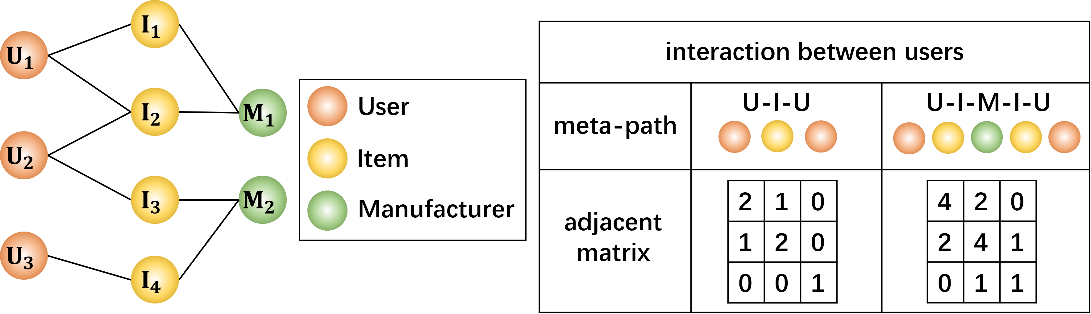
Figure 7: Illustration of dependencies in evolving traffic networks.

6 Conclusion

CL aims to learn new knowledge incrementally without forgetting prior experience, approaches which follow the taxonomy as regularization-based, replay-based and architecture-based (Section 2.1.3). CL mainly focuses on i.i.d data, leaving graph-structural data investigated scarcely. Graphs are widely used to represent relational data (Section 2.2.1), which usually evolve dynamically in real work. DGL aims to capture graph evolution patterns, but it does not focus on overcoming catastrophic forgetting (Section 2.2). CGL is an emerging area realizing CL over evolving graphs (Section 3.1). Graph topology brings along two new challenges: sample-level dependency and graph-level dependency (Section 3.2). Current CGL approaches follow the same taxonomy as CL. However, some merely apply naive CL strategies to graphs, neglecting graph topology (Section 3.5). Novel CL strategies should be proposed to tackle the two challenges. Regularization-based methods should consider which topological information should be preserved and how to encode it (Section 3.7.2). Replay-based approaches are expected to leverage graph topology to guide sampling strategy (Section 3.7.3). Architectural-based methods can analyze parameter importance with respect to graph topology, determining whether to isolate parameters (Section 3.7.4). Furthermore, current CGL tasks mostly study simple GL tasks (e.g., node classification and graph classification), additional research efforts are required to enhance graph robustness, combine CGL with GL models other than GNN, and adapt to more complicated graphs (e.g., multi-model graphs and heterogeneous graphs) (Section 4). Finally, more challenges should be overcome when applying CGL to practical applications (Section 5). We hope that this work could provide some insights for future research.

References

- Ahrabian et al. (2021) Ahrabian K, Xu Y, Zhang Y, Wu J, Wang Y, Coates M (2021) Structure Aware Experience Replay for Incremental Learning in Graph-Based Recommender Systems, 2832–2836 (New York, NY, USA: Association for Computing Machinery).
- Aljundi et al. (2018) Aljundi R, Babiloni F, Elhoseiny M, Rohrbach M, Tuytelaars T (2018) Memory aware synapses: Learning what (not) to forget. Proceedings of the European Conference on Computer Vision (ECCV).
- Aljundi et al. (2019) Aljundi R, Lin M, Goujaud B, Bengio Y (2019) Gradient based sample selection for online continual learning. Wallach H, Larochelle H, Beygelzimer A, d'Alché-Buc F, Fox E, Garnett R, eds., Advances in Neural Information Processing Systems, volume 32 (Curran Associates, Inc.).
- Bai et al. (2018) Bai S, Kolter JZ, Koltun V (2018) An empirical evaluation of generic convolutional and recurrent networks for sequence modeling.
- Bian et al. (2019) Bian R, Koh YS, Dobbie G, Divoli A (2019) Network embedding and change modeling in dynamic heterogeneous networks. Proceedings of the 42nd International ACM SIGIR Conference on Research and Development in Information Retrieval, 861–864, SIGIR’19 (New York, NY, USA: Association for Computing Machinery), ISBN 9781450361729.
- Biesialska et al. (2020) Biesialska M, Biesialska K, Costa-jussà MR (2020) Continual lifelong learning in natural language processing: A survey. Proceedings of the 28th International Conference on Computational Linguistics, 6523–6541 (Barcelona, Spain (Online): International Committee on Computational Linguistics).
- Bojchevski and Günnemann (2017) Bojchevski A, Günnemann S (2017) Deep gaussian embedding of graphs: Unsupervised inductive learning via ranking. arXiv preprint arXiv:1707.03815 .
- Bojchevski et al. (2018) Bojchevski A, Shchur O, Zügner D, Günnemann S (2018) NetGAN: Generating graphs via random walks. Dy J, Krause A, eds., Proceedings of the 35th International Conference on Machine Learning, volume 80 of Proceedings of Machine Learning Research, 610–619 (PMLR).
- Bouritsas et al. (2022) Bouritsas G, Frasca F, Zafeiriou SP, Bronstein M (2022) Improving graph neural network expressivity via subgraph isomorphism counting. IEEE Transactions on Pattern Analysis and Machine Intelligence 1–1.
- Cai et al. (2022) Cai J, Wang X, Guan C, Tang Y, Xu J, Zhong B, Zhu W (2022) Multimodal continual graph learning with neural architecture search. Proceedings of the ACM Web Conference 2022, 1292–1300, WWW ’22 (New York, NY, USA: Association for Computing Machinery).
- Chang et al. (2015) Chang S, Han W, Tang J, Qi GJ, Aggarwal CC, Huang TS (2015) Heterogeneous network embedding via deep architectures. Proceedings of the 21th ACM SIGKDD International Conference on Knowledge Discovery and Data Mining, 119–128, KDD ’15 (New York, NY, USA: Association for Computing Machinery).
- Chaudhry et al. (2019) Chaudhry A, Rohrbach M, Elhoseiny M, Ajanthan T, Dokania PK, Torr PH, Ranzato M (2019) On tiny episodic memories in continual learning. arXiv preprint arXiv:1902.10486 .
- Chen et al. (2018) Chen H, Yin H, Wang W, Wang H, Nguyen QVH, Li X (2018) Pme: Projected metric embedding on heterogeneous networks for link prediction. Proceedings of the 24th ACM SIGKDD International Conference on Knowledge Discovery & Data Mining, 1177–1186, KDD ’18 (New York, NY, USA: Association for Computing Machinery).
- Chen et al. (2022) Chen J, Wang X, Xu X (2022) Gc-lstm: graph convolution embedded lstm for dynamic network link prediction. Applied Intelligence 52, ISSN 1573-7497.
- Chen et al. (2021) Chen X, Wang J, Xie K (2021) Trafficstream: A streaming traffic flow forecasting framework based on graph neural networks and continual learning. Zhou ZH, ed., Proceedings of the Thirtieth International Joint Conference on Artificial Intelligence, IJCAI-21, 3620–3626 (International Joint Conferences on Artificial Intelligence Organization), main Track.
- Chen et al. (2020) Chen Y, Bian Y, Xiao X, Rong Y, Xu T, Huang J (2020) On self-distilling graph neural network.
- Cheng et al. (2022) Cheng D, Yang F, Xiang S, Liu J (2022) Financial time series forecasting with multi-modality graph neural network. Pattern Recognition 121:108218.
- Chouard and Tanguy (2016) Chouard, Tanguy (2016) The go files: Ai computer wraps up 4-1 victory against human champion. Nature 102(3):419–457.
- de Bruin et al. (2016) de Bruin T, Kober J, Tuyls K, Babuška R (2016) Improved deep reinforcement learning for robotics through distribution-based experience retention. 2016 IEEE/RSJ International Conference on Intelligent Robots and Systems (IROS), 3947–3952.
- de Masson d'Autume et al. (2019) de Masson d'Autume C, Ruder S, Kong L, Yogatama D (2019) Episodic memory in lifelong language learning. Wallach H, Larochelle H, Beygelzimer A, d'Alché-Buc F, Fox E, Garnett R, eds., Advances in Neural Information Processing Systems, volume 32 (Curran Associates, Inc.).
- Delange et al. (2021) Delange M, Aljundi R, Masana M, Parisot S, Jia X, Leonardis A, Slabaugh G, Tuytelaars T (2021) A continual learning survey: Defying forgetting in classification tasks. IEEE Transactions on Pattern Analysis and Machine Intelligence 1–1.
- Deng and Zhang (2021) Deng X, Zhang Z (2021) Graph-free knowledge distillation for graph neural networks.
- Dettmers et al. (2018) Dettmers T, Minervini P, Stenetorp P, Riedel S (2018) Convolutional 2d knowledge graph embeddings. Proceedings of the AAAI conference on artificial intelligence, volume 32.
- Ding et al. (2022) Ding S, Feng F, He X, Liao Y, Shi J, Zhang Y (2022) Causal incremental graph convolution for recommender system retraining. IEEE Transactions on Neural Networks and Learning Systems 1–11.
- Farajtabar et al. (2020) Farajtabar M, Azizan N, Mott A, Li A (2020) Orthogonal gradient descent for continual learning. Chiappa S, Calandra R, eds., Proceedings of the Twenty Third International Conference on Artificial Intelligence and Statistics, volume 108 of Proceedings of Machine Learning Research, 3762–3773 (PMLR).
- Febrinanto et al. (2022) Febrinanto FG, Xia F, Moore K, Thapa C, Aggarwal C (2022) Graph lifelong learning: A survey. URL http://dx.doi.org/10.48550/ARXIV.2202.10688.
- Fernando et al. (2017) Fernando C, Banarse D, Blundell C, Zwols Y, Ha D, Rusu AA, Pritzel A, Wierstra D (2017) Pathnet: Evolution channels gradient descent in super neural networks. CoRR abs/1701.08734.
- Finn et al. (2017) Finn C, Abbeel P, Levine S (2017) Model-agnostic meta-learning for fast adaptation of deep networks. Precup D, Teh YW, eds., Proceedings of the 34th International Conference on Machine Learning, volume 70 of Proceedings of Machine Learning Research, 1126–1135 (PMLR).
- Galke et al. (2021) Galke L, Franke B, Zielke T, Scherp A (2021) Lifelong learning of graph neural networks for open-world node classification. 2021 International Joint Conference on Neural Networks (IJCNN), 1–8.
- Gao and Ji (2019) Gao H, Ji S (2019) Graph u-nets. Chaudhuri K, Salakhutdinov R, eds., Proceedings of the 36th International Conference on Machine Learning, volume 97 of Proceedings of Machine Learning Research, 2083–2092 (PMLR).
- Gao et al. (2021) Gao H, Liu Y, Ji S (2021) Topology-aware graph pooling networks. IEEE Transactions on Pattern Analysis and Machine Intelligence 43(12):4512–4518, URL http://dx.doi.org/10.1109/TPAMI.2021.3062794.
- Gao et al. (2019) Gao Y, Yang H, Zhang P, Zhou C, Hu Y (2019) Graphnas: Graph neural architecture search with reinforcement learning. arXiv preprint arXiv:1904.09981 .
- Grossberg (1982) Grossberg S (1982) Studies of mind and brain neural principles of learning, perception, development, cognition, and motor control. Boston Studies in the Philosophy of Science 70.
- Hamilton et al. (2017) Hamilton W, Ying Z, Leskovec J (2017) Inductive representation learning on large graphs. Guyon I, Luxburg UV, Bengio S, Wallach H, Fergus R, Vishwanathan S, Garnett R, eds., Advances in Neural Information Processing Systems, volume 30 (Curran Associates, Inc.).
- Hampel et al. (2011) Hampel FR, Ronchetti EM, Rousseeuw PJ, Stahel WA (2011) Robust statistics: the approach based on influence functions, volume 196 (John Wiley & Sons).
- Han et al. (2020) Han Y, Karunasekera S, Leckie C (2020) Graph neural networks with continual learning for fake news detection from social media.
- He et al. (2015) He K, Zhang X, Ren S, Sun J (2015) Delving deep into rectifiers: Surpassing human-level performance on imagenet classification. Proceedings of the IEEE International Conference on Computer Vision (ICCV).
- Hecht-Nielsen (1992) Hecht-Nielsen R (1992) Theory of the backpropagation neural network. Neural networks for perception, 65–93 (Elsevier).
- Hinton et al. (2015) Hinton G, Vinyals O, Dean J (2015) Distilling the knowledge in a neural network. NIPS Deep Learning and Representation Learning Workshop.
- Horn et al. (2021) Horn M, Brouwer ED, Moor M, Moreau Y, Rieck B, Borgwardt KM (2021) Topological graph neural networks. CoRR abs/2102.07835.
- Hsu et al. (2017) Hsu CC, Lai YA, Chen WH, Feng MH, Lin SD (2017) Unsupervised ranking using graph structures and node attributes. Proceedings of the Tenth ACM International Conference on Web Search and Data Mining, 771–779, WSDM ’17 (New York, NY, USA: Association for Computing Machinery), ISBN 9781450346757.
- Huang et al. (2014) Huang R, Sakamuru S, Martin MT, Reif DM, Judson RS, Houck KA, Casey W, Hsieh JH, Shockley KR, Ceger P, et al. (2014) Profiling of the tox21 10k compound library for agonists and antagonists of the estrogen receptor alpha signaling pathway. Scientific reports 4(1):1–9.
- Isele and Cosgun (2018) Isele D, Cosgun A (2018) Selective experience replay for lifelong learning. Proceedings of the AAAI Conference on Artificial Intelligence 32(1).
- Jha et al. (2021) Jha K, Xun G, Zhang A (2021) Continual representation learning for evolving biomedical bipartite networks. Bioinformatics 37(15):2190–2197.
- Jin et al. (2020) Jin W, Li Y, Xu H, Wang Y, Ji S, Aggarwal C, Tang J (2020) Adversarial attacks and defenses on graphs: A review, a tool and empirical studies. URL http://dx.doi.org/10.48550/ARXIV.2003.00653.
- Kirkpatrick et al. (2017) Kirkpatrick J, Pascanu R, Rabinowitz N, Veness J, Desjardins G, Rusu AA, Milan K, Quan J, Ramalho T, Grabska-Barwinska A, Hassabis D, Clopath C, Kumaran D, Hadsell R (2017) Overcoming catastrophic forgetting in neural networks. Proceedings of the National Academy of Sciences 114(13):3521–3526.
- Kleinberg (1999) Kleinberg JM (1999) Authoritative sources in a hyperlinked environment. J. ACM 46(5):604–632, ISSN 0004-5411.
- Kleinberg et al. (1999) Kleinberg JM, Kumar R, Raghavan P, Rajagopalan S, Tomkins AS (1999) The web as a graph: Measurements, models, and methods. International Computing and Combinatorics Conference, 1–17 (Springer).
- Koh and Liang (2017) Koh PW, Liang P (2017) Understanding black-box predictions via influence functions. Precup D, Teh YW, eds., Proceedings of the 34th International Conference on Machine Learning, volume 70 of Proceedings of Machine Learning Research, 1885–1894 (PMLR).
- Kou et al. (2020) Kou X, Lin Y, Liu S, Li P, Zhou J, Zhang Y (2020) Disentangle-based continual graph representation learning.
- Lee et al. (2019) Lee J, Lee I, Kang J (2019) Self-attention graph pooling. Chaudhuri K, Salakhutdinov R, eds., Proceedings of the 36th International Conference on Machine Learning, volume 97 of Proceedings of Machine Learning Research, 3734–3743 (PMLR).
- Li et al. (2022) Li H, Zhang J, Yang L, Qi J, Gao Z (2022) Graph-gan: A spatial-temporal neural network for short-term passenger flow prediction in urban rail transit systems. arXiv preprint arXiv:2202.06727 .
- Li et al. (2017) Li J, Dani H, Hu X, Tang J, Chang Y, Liu H (2017) Attributed network embedding for learning in a dynamic environment. Proceedings of the 2017 ACM on Conference on Information and Knowledge Management, 387–396, CIKM ’17 (New York, NY, USA: Association for Computing Machinery), ISBN 9781450349185.
- Li and Hoiem (2018) Li Z, Hoiem D (2018) Learning without forgetting. IEEE Transactions on Pattern Analysis and Machine Intelligence 40(12):2935–2947.
- Liu et al. (2021) Liu H, Yang Y, Wang X (2021) Overcoming catastrophic forgetting in graph neural networks. Proceedings of the AAAI Conference on Artificial Intelligence 35(10):8653–8661.
- Lopez-Paz and Ranzato (2017) Lopez-Paz D, Ranzato MA (2017) Gradient episodic memory for continual learning. Guyon I, Luxburg UV, Bengio S, Wallach H, Fergus R, Vishwanathan S, Garnett R, eds., Advances in Neural Information Processing Systems, volume 30 (Curran Associates, Inc.).
- Mahadevan et al. (2006) Mahadevan P, Krioukov D, Fall K, Vahdat A (2006) Systematic topology analysis and generation using degree correlations. 135–146, SIGCOMM ’06 (New York, NY, USA: Association for Computing Machinery), ISBN 1595933085.
- Mallya et al. (2018) Mallya A, Davis D, Lazebnik S (2018) Piggyback: Adapting a single network to multiple tasks by learning to mask weights. Proceedings of the European Conference on Computer Vision (ECCV).
- McCloskey and Cohen (1989) McCloskey M, Cohen NJ (1989) Catastrophic interference in connectionist networks: The sequential learning problem. volume 24 of Psychology of Learning and Motivation, 109–165 (Academic Press).
- Mermillod et al. (2013) Mermillod M, Bugaiska A, BONIN P (2013) The stability-plasticity dilemma: investigating the continuum from catastrophic forgetting to age-limited learning effects. Frontiers in Psychology 4, ISSN 1664-1078.
- Nagy and Simon (2018) Nagy AM, Simon V (2018) Survey on traffic prediction in smart cities. Pervasive and Mobile Computing 50:148–163, ISSN 1574-1192.
- Ostapenko et al. (2019) Ostapenko O, Puscas M, Klein T, Jahnichen P, Nabi M (2019) Learning to remember: A synaptic plasticity driven framework for continual learning. Proceedings of the IEEE/CVF Conference on Computer Vision and Pattern Recognition (CVPR).
- Page et al. (1999) Page L, Brin S, Motwani R, Winograd T (1999) The pagerank citation ranking: Bringing order to the web. Technical report, Stanford InfoLab.
- Pareja et al. (2020) Pareja A, Domeniconi G, Chen J, Ma T, Suzumura T, Kanezashi H, Kaler T, Schardl T, Leiserson C (2020) Evolvegcn: Evolving graph convolutional networks for dynamic graphs. Proceedings of the AAAI Conference on Artificial Intelligence 34(04):5363–5370.
- Parisi et al. (2019) Parisi GI, Kemker R, Part JL, Kanan C, Wermter S (2019) Continual lifelong learning with neural networks: A review. Neural Networks 113:54–71, ISSN 0893-6080.
- Perini et al. (2022) Perini M, Ramponi G, Carbone P, Kalavri V (2022) Learning on streaming graphs with experience replay. Proceedings of the 37th ACM/SIGAPP Symposium on Applied Computing, 470–478, SAC ’22 (New York, NY, USA: Association for Computing Machinery).
- Perozzi et al. (2014) Perozzi B, Al-Rfou R, Skiena S (2014) Deepwalk: Online learning of social representations. 701–710, KDD ’14 (New York, NY, USA: Association for Computing Machinery).
- Rannen et al. (2017) Rannen A, Aljundi R, Blaschko MB, Tuytelaars T (2017) Encoder based lifelong learning. Proceedings of the IEEE International Conference on Computer Vision (ICCV).
- Rebuffi et al. (2017) Rebuffi SA, Kolesnikov A, Sperl G, Lampert CH (2017) icarl: Incremental classifier and representation learning. Proceedings of the IEEE Conference on Computer Vision and Pattern Recognition (CVPR).
- Rendsburg et al. (2020) Rendsburg L, Heidrich H, Luxburg UV (2020) NetGAN without GAN: From random walks to low-rank approximations. III HD, Singh A, eds., Proceedings of the 37th International Conference on Machine Learning, volume 119 of Proceedings of Machine Learning Research, 8073–8082 (PMLR).
- Rolnick et al. (2019) Rolnick D, Ahuja A, Schwarz J, Lillicrap T, Wayne G (2019) Experience replay for continual learning. Wallach H, Larochelle H, Beygelzimer A, d'Alché-Buc F, Fox E, Garnett R, eds., Advances in Neural Information Processing Systems, volume 32 (Curran Associates, Inc.).
- Ruhnau (2000) Ruhnau B (2000) Eigenvector-centrality — a node-centrality? Social Networks 22(4):357–365, ISSN 0378-8733.
- Rusu et al. (2016) Rusu AA, Rabinowitz NC, Desjardins G, Soyer H, Kirkpatrick J, Kavukcuoglu K, Pascanu R, Hadsell R (2016) Progressive neural networks.
- Sankar et al. (2020) Sankar A, Wu Y, Gou L, Zhang W, Yang H (2020) Dysat: Deep neural representation learning on dynamic graphs via self-attention networks. Proceedings of the 13th International Conference on Web Search and Data Mining, 519–527, WSDM ’20 (New York, NY, USA: Association for Computing Machinery), ISBN 9781450368223.
- Sen et al. (2008) Sen P, Namata G, Bilgic M, Getoor L, Galligher B, Eliassi-Rad T (2008) Collective classification in network data. AI Magazine 29(3):93, URL http://dx.doi.org/10.1609/aimag.v29i3.2157.
- Serra et al. (2018) Serra J, Suris D, Miron M, Karatzoglou A (2018) Overcoming catastrophic forgetting with hard attention to the task. Dy J, Krause A, eds., Proceedings of the 35th International Conference on Machine Learning, volume 80 of Proceedings of Machine Learning Research, 4548–4557 (PMLR).
- Shi et al. (2018) Shi Y, Zhu Q, Guo F, Zhang C, Han J (2018) Easing embedding learning by comprehensive transcription of heterogeneous information networks. Proceedings of the 24th ACM SIGKDD International Conference on Knowledge Discovery & Data Mining, 2190–2199, KDD ’18 (New York, NY, USA: Association for Computing Machinery).
- Shin et al. (2017) Shin H, Lee JK, Kim J, Kim J (2017) Continual learning with deep generative replay. Guyon I, Luxburg UV, Bengio S, Wallach H, Fergus R, Vishwanathan S, Garnett R, eds., Advances in Neural Information Processing Systems, volume 30 (Curran Associates, Inc.).
- Sokar et al. (2021) Sokar G, Mocanu DC, Pechenizkiy M (2021) Spacenet: Make free space for continual learning. Neurocomputing 439:1–11.
- Sun et al. (2022) Sun L, Ye J, Peng H, Wang F, Yu PS (2022) Self-supervised continual graph learning in adaptive riemannian spaces. arXiv preprint arXiv:2211.17068 .
- Sussmann (1992) Sussmann HJ (1992) Uniqueness of the weights for minimal feedforward nets with a given input-output map. Neural Networks 5(4):589–593, ISSN 0893-6080.
- Tan et al. (2022) Tan Z, Ding K, Guo R, Liu H (2022) Graph few-shot class-incremental learning. Proceedings of the Fifteenth ACM International Conference on Web Search and Data Mining, 987–996, WSDM ’22 (New York, NY, USA: Association for Computing Machinery), ISBN 9781450391320.
- Tang et al. (2008) Tang J, Zhang J, Yao L, Li J, Zhang L, Su Z (2008) Arnetminer: extraction and mining of academic social networks. Proceedings of the 14th ACM SIGKDD international conference on Knowledge discovery and data mining, 990–998.
- Tao et al. (2020) Tao Z, Wei Y, Wang X, He X, Huang X, Chua TS (2020) Mgat: Multimodal graph attention network for recommendation. Information Processing & Management 57(5):102277.
- Tian et al. (2022) Tian H, Zheng X, Zhao K, Liu MW, Zeng DD (2022) Inductive representation learning on dynamic stock co-movement graphs for stock predictions. INFORMS Journal on Computing .
- Toutanova and Chen (2015) Toutanova K, Chen D (2015) Observed versus latent features for knowledge base and text inference. Proceedings of the 3rd workshop on continuous vector space models and their compositionality, 57–66.
- Veličković et al. (2018) Veličković P, Cucurull G, Casanova A, Romero A, Liò P, Bengio Y (2018) Graph attention networks. International Conference on Learning Representations.
- Wang et al. (2022a) Wang C, Qiu Y, Gao D, Scherer S (2022a) Lifelong graph learning. Proceedings of the IEEE/CVF Conference on Computer Vision and Pattern Recognition (CVPR), 13719–13728.
- Wang et al. (2020) Wang J, Song G, Wu Y, Wang L (2020) Streaming graph neural networks via continual learning. 1515–1524, CIKM ’20 (New York, NY, USA: Association for Computing Machinery).
- Wang et al. (2021a) Wang J, Zhang S, Xiao Y, Song R (2021a) A review on graph neural network methods in financial applications. arXiv preprint arXiv:2111.15367 .
- Wang et al. (2022b) Wang J, Zhu W, Song G, Wang L (2022b) Streaming graph neural networks with generative replay. Proceedings of the 28th ACM SIGKDD Conference on Knowledge Discovery and Data Mining, 1878–1888, KDD ’22 (New York, NY, USA: Association for Computing Machinery), ISBN 9781450393850.
- Wang et al. (2022c) Wang X, Bo D, Shi C, Fan S, Ye Y, Yu PS (2022c) A survey on heterogeneous graph embedding: Methods, techniques, applications and sources. IEEE Transactions on Big Data 1–1.
- Wang et al. (2022d) Wang X, Lu Y, Shi C, Wang R, Cui P, Mou S (2022d) Dynamic heterogeneous information network embedding with meta-path based proximity. IEEE Transactions on Knowledge and Data Engineering 34(3):1117–1132.
- Wang et al. (2022e) Wang X, Lu Y, Shi C, Wang R, Cui P, Mou S (2022e) Dynamic heterogeneous information network embedding with meta-path based proximity. IEEE Transactions on Knowledge and Data Engineering 34(3):1117–1132.
- Wang et al. (2021b) Wang Y, Zhang Y, Coates M (2021b) Graph Structure Aware Contrastive Knowledge Distillation for Incremental Learning in Recommender Systems, 3518–3522 (New York, NY, USA: Association for Computing Machinery), ISBN 9781450384469.
- Wei et al. (2019) Wei Y, Wang X, Nie L, He X, Hong R, Chua TS (2019) Mmgcn: Multi-modal graph convolution network for personalized recommendation of micro-video. Proceedings of the 27th ACM International Conference on Multimedia, 1437–1445, MM ’19 (New York, NY, USA: Association for Computing Machinery), ISBN 9781450368896.
- Wu et al. (2018) Wu Z, Ramsundar B, Feinberg EN, Gomes J, Geniesse C, Pappu AS, Leswing K, Pande V (2018) Moleculenet: a benchmark for molecular machine learning. Chemical science 9(2):513–530.
- Xia et al. (2021a) Xia F, Sun K, Yu S, Aziz A, Wan L, Pan S, Liu H (2021a) Graph learning: A survey. IEEE Transactions on Artificial Intelligence 2(2):109–127.
- Xia et al. (2021b) Xia J, Li D, Gu H, Lu T, Zhang P, Gu N (2021b) Incremental Graph Convolutional Network for Collaborative Filtering, 2170–2179 (New York, NY, USA: Association for Computing Machinery).
- Xing and Ghorbani (2004) Xing W, Ghorbani A (2004) Weighted pagerank algorithm. Proceedings. Second Annual Conference on Communication Networks and Services Research, 2004., 305–314, URL http://dx.doi.org/10.1109/DNSR.2004.1344743.
- Xu et al. (2020a) Xu H, Ma Y, Liu HC, Deb D, Liu H, Tang JL, Jain AK (2020a) Adversarial attacks and defenses in images, graphs and text: A review. International Journal of Automation and Computing 17(2):151–178.
- Xu et al. (2020b) Xu Y, Zhang Y, Guo W, Guo H, Tang R, Coates M (2020b) Graphsail: Graph structure aware incremental learning for recommender systems. Proceedings of the 29th ACM International Conference on Information & Knowledge Management, 2861–2868, CIKM ’20 (New York, NY, USA: Association for Computing Machinery), ISBN 9781450368599.
- Xue et al. (2022) Xue G, Zhong M, Li J, Chen J, Zhai C, Kong R (2022) Dynamic network embedding survey. Neurocomputing 472:212–223, ISSN 0925-2312.
- Xue et al. (2021) Xue H, Yang L, Jiang W, Wei Y, Hu Y, Lin Y (2021) Modeling dynamic heterogeneous network for link prediction using hierarchical attention with temporal rnn. Hutter F, Kersting K, Lijffijt J, Valera I, eds., Machine Learning and Knowledge Discovery in Databases, 282–298 (Cham: Springer International Publishing).
- Ye et al. (2020) Ye J, Zhao J, Ye K, Xu C (2020) How to build a graph-based deep learning architecture in traffic domain: A survey. IEEE Transactions on Intelligent Transportation Systems 1–21.
- Yim et al. (2017) Yim J, Joo D, Bae J, Kim J (2017) A gift from knowledge distillation: Fast optimization, network minimization and transfer learning. Proceedings of the IEEE Conference on Computer Vision and Pattern Recognition (CVPR).
- Ying et al. (2018) Ying Z, You J, Morris C, Ren X, Hamilton W, Leskovec J (2018) Hierarchical graph representation learning with differentiable pooling. Bengio S, Wallach H, Larochelle H, Grauman K, Cesa-Bianchi N, Garnett R, eds., Advances in Neural Information Processing Systems, volume 31 (Curran Associates, Inc.).
- Yoon et al. (2018) Yoon J, Yang E, Lee J, Hwang SJ (2018) Lifelong learning with dynamically expandable networks. International Conference on Learning Representations.
- Yu et al. (2018) Yu B, Yin H, Zhu Z (2018) Spatio-temporal graph convolutional networks: A deep learning framework for traffic forecasting. Proceedings of the 27th International Joint Conference on Artificial Intelligence, 3634–3640, IJCAI’18 (AAAI Press), ISBN 9780999241127.
- Yuan and Ji (2020) Yuan H, Ji S (2020) Structpool: Structured graph pooling via conditional random fields. International Conference on Learning Representations.
- Zenke et al. (2017) Zenke F, Poole B, Ganguli S (2017) Continual learning through synaptic intelligence. Precup D, Teh YW, eds., Proceedings of the 34th International Conference on Machine Learning, volume 70 of Proceedings of Machine Learning Research, 3987–3995 (PMLR).
- Zhang et al. (2019a) Zhang C, Song D, Huang C, Swami A, Chawla NV (2019a) Heterogeneous graph neural network. Proceedings of the 25th ACM SIGKDD International Conference on Knowledge Discovery & Data Mining, 793–803, KDD ’19 (New York, NY, USA: Association for Computing Machinery), ISBN 9781450362016.
- Zhang and Luo (2017) Zhang J, Luo Y (2017) Degree centrality, betweenness centrality, and closeness centrality in social network. 2017 2nd International Conference on Modelling, Simulation and Applied Mathematics (MSAM2017), 300–303 (Atlantis Press).
- Zhang et al. (2020) Zhang J, Zhang J, Ghosh S, Li D, Tasci S, Heck L, Zhang H, Kuo CCJ (2020) Class-incremental learning via deep model consolidation. Proceedings of the IEEE/CVF Winter Conference on Applications of Computer Vision (WACV).
- Zhang et al. (2022a) Zhang X, Song D, Tao D (2022a) Hierarchical prototype networks for continual graph representation learning. IEEE Transactions on Pattern Analysis and Machine Intelligence 1–15.
- Zhang et al. (2007) Zhang X, Yu H, Zhang C, Liu X (2007) An improved weighted hits algorithm based on similarity andpopularity. Second International Multi-Symposiums on Computer and Computational Sciences (IMSCCS 2007), 477–480.
- Zhang et al. (2019b) Zhang Z, Bu J, Ester M, Zhang J, Yao C, Yu Z, Wang C (2019b) Hierarchical graph pooling with structure learning. URL http://dx.doi.org/10.48550/ARXIV.1911.05954.
- Zhang et al. (2022b) Zhang Z, Cui P, Zhu W (2022b) Deep learning on graphs: A survey. IEEE Transactions on Knowledge and Data Engineering 34(1):249–270.
- Zhao et al. (2020) Zhao L, Song Y, Zhang C, Liu Y, Wang P, Lin T, Deng M, Li H (2020) T-gcn: A temporal graph convolutional network for traffic prediction. IEEE Transactions on Intelligent Transportation Systems 21(9):3848–3858.
- Zhou et al. (2020) Zhou D, Zheng L, Han J, He J (2020) A data-driven graph generative model for temporal interaction networks. Proceedings of the 26th ACM SIGKDD International Conference on Knowledge Discovery & Data Mining, 401–411, KDD ’20 (New York, NY, USA: Association for Computing Machinery).
- Zhou and Cao (2021) Zhou F, Cao C (2021) Overcoming catastrophic forgetting in graph neural networks with experience replay. Proceedings of the AAAI Conference on Artificial Intelligence 35(5):4714–4722.
- Zitnik and Leskovec (2017) Zitnik M, Leskovec J (2017) Predicting multicellular function through multi-layer tissue networks. Bioinformatics 33(14):i190–i198, ISSN 1367-4803, URL http://dx.doi.org/10.1093/bioinformatics/btx252.