The first variation of the matter energy-momentum tensor with respect to the metric, and its implications on modified gravity theories

Abstract

The first order variation of the matter energy-momentum tensor $T_{\mu\nu}$ with respect to the metric tensor $g^{\alpha\beta}$ plays an important role in modified gravity theories with geometry-matter coupling, and in particular in the $f(R,T)$ modified gravity theory. We obtain the expression of the variation $\delta T_{\mu\nu}/\delta g^{\alpha\beta}$ for the baryonic matter described by an equation given in a parametric form, with the basic thermodynamic variables represented by the particle number density, and by the specific entropy, respectively. The first variation of the matter energy-momentum tensor turns out to be independent on the matter Lagrangian, and can be expressed in terms of the pressure, the energy-momentum tensor itself, and the matter fluid four-velocity. We apply the obtained results for the case of the $f(R,T)$ gravity theory, where $R$ is the Ricci scalar, and $T$ is the trace of the matter energy-momentum tensor, which thus becomes a unique theory, also independent on the choice of the matter Lagrangian. A simple cosmological model, in which the Hilbert-Einstein Lagrangian is generalized through the addition of a term proportional to $T^{n}$ is considered in detail, and it is shown that it gives a very good description of the observational values of the Hubble parameter up to a redshift of $z\approx 2.5$.

I Introduction

There are at least three theoretical perspectives that could be used to explain the large amount of recent observations, which strongly suggest a faster and faster expanding Universe [2, 3], with a composition in which ordinary matter represents only 5% of its composition, the rest being represented by the dark energy, and the dark matter [3, 4]. The first point of view is represented by the dark constituents theory, which adds two more components to the total energy momentum tensor of the Universe, representing dark matter and dark energy, respectively. Therefore the cosmological dynamics is described by the field equation $G_{\mu\nu}=\kappa^{2}T^{\rm bar}_{\mu\nu}+\kappa^{2}T^{\rm DM}_{\mu\nu}(\phi,\psi_{\mu},...)+\kappa^{2}T^{\rm DE}_{\mu\nu}(\phi,\psi_{\mu},...)$, where $T^{\rm bar}_{\mu\nu}$, $T^{\rm DM}_{\mu\nu}(\phi,\psi_{\mu},...)$, and $T^{\rm DE}_{\mu\nu}(\phi,\psi_{\mu},...)$ represent the energy-momentum tensors of baryonic matter, dark matter, and dark energy, respectively, with $\phi$ and $\psi_{\mu}$ representing scalar or vector fields. A well studied dark constituent model is represented by the quintessence (scalar field) description of dark energy [5, 6].

In the dark geometry approach, an exclusively geometric attitude on the gravitational phenomena is adopted, by explaining the cosmological dynamics through the modification of the geometry underlying the Einstein field equations. Hence, the extended Einstein equations become in this approach $G_{\mu\nu}=\kappa^{2}T_{\mu\nu}^{{\rm bar}}+\kappa^{2}T_{\mu\nu}^{(\rm geom)}\left(g_{\mu\nu},R,\square R,...\right)$, where $T_{\mu\nu}$ is the energy-momentum tensor of ordinary matter, and $T_{\mu\nu}^{(\rm geom)}\left(g_{\mu\nu},R,\square R,...\right)$ is a purely geometric term, obtained from the metric, torsion $\tau$, nonmetricity $Q$, extensions of Riemann geometry etc., and which can effectively mimic dark energy, dark matter, or both. Some typical example of dark geometric theories are the $f(R)$ [7], $f(Q)$ [8], hybrid metric-Palatini gravity [9] theories, or gravitational theories based on the Weyl-Cartan-Weitzenböck [10] and Finsler geometries [11, 12].

The third avenue for the understanding of the gravitational and cosmological phenomena is represented by the dark coupling approach, in which the standard Einstein gravitational equations are generalized to take the mathematical form $G_{\mu\nu}=\kappa^{2}T_{\mu\nu}+\kappa^{2}T_{\mu\nu}^{(\rm coup)}\left(R,L_{m},T,\square R,\square T,...\right)$, where the effective energy-momentum tensor $T_{\mu\nu}^{(\rm coup)}\left(g_{\mu\nu},R,L_{m},T,\square R,\square T,...\right)$ of the theory is built up by considering the maximal extension of the Hilbert-Einstein Lagrangian, by abandoning its additive structure in matter and geometry. In the dark coupling approach, matter is represented either by the trace $T$ of the matter energy-momentum tensor, by the matter Lagrangian $L_{m}$ or by some scalar made by $T_{\mu\nu}$ such as $T_{\mu\nu}T^{\mu\nu}$.

The dark coupling approach is also a theoretical answer to the problem of the maximal extension of the additive Hilbert-Einstein Lagrangian, which automatically implies a non-additive structure of the action in the geometric and matter variables. In a general form the requirement of the maximal extension of the gravitational action can be implemented by assuming that the Lagrangian of the gravitational field is an arbitrary function of the curvature scalar $R$, and of the matter Lagrangian $L_{m}$. One of the interesting features of the dark coupling models is that they imply the presence of a nonminimal geometry-matter coupling. Dark couplings are not restricted to Riemannian geometry, but they can be considered in the framework of the extensions of Riemann geometry. Typical examples of dark coupling theories are the $f\left(R,L_{m}\right)$ [13, 14], $f(R,T)$ [15], $f\left(R,T,R_{\mu\nu}T^{\mu\nu}\right)$ [16], $f(\tau,T)$ [17], $f(Q,T)$ [18], or the $f\left(R,T,Q,T_{m}\right)$ [19] theories.

One of the interesting consequences of the dark coupling theories is the reconsideration of the role of the ordinary (baryonic) matter in the cosmological dynamics. Through its coupling to gravity, matter becomes a key element in the explanation of cosmic dynamics, and recovers its central role gravity, which is minimized or even neglected in the dark constituents and dark geometric type theories. An important implication of the geometry-matter coupling is that the matter energy-momentum tensor is generally not conserved, and thus an extra-force is generated, acting on massive particles moving in a gravitational field, with the particles following non-geodesic paths [14, 15]. The possibility of the existence of such couplings between matter and geometry have opened interesting, and novel pathways for the study of gravitational phenomena [20].

However, the dependence of the gravitational action in the dark coupling theories on $L_{m}$ gives a new relevance to the old problem of the degeneracy of the matter Lagrangian. Two, physically inequivalent expressions of the matter Lagrangian, $L_{m}=-\rho$, and $L_{m}=P$, lead to the same energy-momentum tensor for matter. This result has important implications for dark coupling gravity models. For example, in the framework of the $f\left(R,L_{m}\right)$ theory, it was shown in [21] that adopting for the Lagrangian density the expression $L_{m}=p$, where $p$ is the pressure, in the case of dust the extra force vanishes. However, for the form $L_{m}=\rho$ of the matter Lagrangian, the extra-force does not vanish [22]. In [23] it was shown, by using the variational formulation for the derivation of the equations of motion, that both the matter Lagrangian, and the energy-momentum tensor, are uniquely and completely determined by the form of the geometry-matter coupling. Therefore, the extra-force never vanishes as a consequence of the thermodynamic properties of the system. In [24] it was shown that if the particle number is conserved, the Lagrangian of a barotropic perfect fluid with $P=P(\rho)$ is $L_{m}=-\rho\left[c^{2}+\int{P(\rho)/\rho^{2}d\rho}\right]$, where $\rho$ is the rest mass density. This result can be used successfully in the study of the modified theories of gravity. The result is based on the assumption that the Lagrangian does not depend on the derivatives of the metric, and that the particle number of the fluid is a conserved quantity, $\nabla_{\mu}\left(\rho u^{\mu}\right)=0$. The matter Lagrangian also plays an important role in the $f(R,T)$ theory of gravity [15].

In theories with geometry-matter coupling another important quantity, the variation of the energy-momentum tensor with respect to the metric does appear, and plays an important role. The corresponding second order tensor is denoted as $\mathbb{T}_{\mu\nu}$, and it is introduced via the definition [15]

$$\mathbb{T}_{\mu\nu}\equiv g^{\rho\sigma}\frac{\delta T_{\rho\sigma}}{\delta g^{\mu\nu}}.$$

If the matter Lagrangian does not depend on the derivatives of the metric, one can obtain for $\mathbb{T}_{\mu\nu}$ a mathematical expression that also contains the second variation of the matter Lagrangian with respect to the metric, $\delta^{2}L_{m}/\delta g^{\mu\nu}\delta g^{\alpha\beta}$. The Lagrangian of the electromagnetic field is quadratic in the components of the metric tensor, and hence its second variation gives a non-zero contribution to $\mathbb{T}_{\mu\nu}$. However, the case of ordinary baryonic matter is more complicated. At first sight, by taking into account the explicit forms of the matter Lagrangians, $L_{m}=-\rho$, or $L_{m}=p$, no explicit dependence on the metric does appear, as opposed, for example, to the case of the electromagnetic field. This would suggest that the second variation of the matter Lagrangian always identically vanishes, no matter what its functional form is. This conclusion may be valid indeed for some special forms of the equation of state, but it is not correct if one adopts a general thermodynamic description of the baryonic fluids.

It is the goal of the present Letter to investigate the problem of the second variation of the perfect fluid matter Lagrangian with respect to the metric tensor components, and to analyze its impact on modified gravity theories. As a first step in our analysis, we obtain, from general thermodynamic considerations, the expressions of the variations with respect to the metric and of the baryonic matter energy density and pressure. Once these expressions are known, a straightforward calculation, involving the computation of the second variation of the energy density and pressure, gives the first variation of the matter energy-momentum tensor with respect to the metric, which also allows to obtain the tensor $\mathbb{T}_{\mu\nu}$. The basic result of our investigation is that the tensor $\mathbb{T}_{\mu\nu}$ is independent of the choice of the matter Lagrangian. The effect of the second order correction is estimated in a cosmological background. As a specific example we will concentrate on the $f(R,T)$ gravity theory, in which the tensor $\mathbb{T}_{\mu\nu}$ plays an important role.

The present Letter is organized as follows. The general thermodynamic formalism used for the calculation of the second variation of the matter Lagrangian is discussed in Section II. The general expression for the second variation of the matter Lagrangian, and of the variation of the energy-momentum tensor is presented in Section III. Some cosmological applications of the obtained results are presented in Section III.1. We then briefly review the basics of the $f(R,T)$ gravity theory in Section IV and outline its cosmological implications for a simple choice $f(R,T)=\alpha|T|^{n}$. Finally, we discuss and conclude our results in Section V.

II Thermodynamics and geometry

In order to obtain the second variation of the baryonic matter Lagrangian, it is necessary to review the derivation of its first variation using thermodynamics considerations. The first law of the thermodynamic is given by

$$dU=TdS-PdV+\mu dN,$$ (1)

where $U$ is the total energy, $\mu$ is the chemical potential, related to the change in the number of particles in the system, $N$ is the particle number and $V$ is the volume enclosing the fluid. An important thermodynamic relation is the Gibbs-Duhem equation,

$$U=TS-PV+\mu N,$$ (2)

which follows from the extensivity of the energy, $U(\lambda X)=\lambda U(X)$, where $\lambda$ is a constant, and from Euler’s theorem of the homogeneous functions.

Let us define the particle number density $n=N/V$ and entropy per particle $s=S/N$. The first law of thermodynamics (1) and the Gibbs-Duhem relation (2) can be simplified to [25]

$$d\rho =Tnds+\mu^{\prime}dn,$$ (3)

$$\rho =\mu^{\prime}n-P,$$ (4)

where $\mu^{\prime}=\mu+Ts$ and we have defined the energy density as $\rho=U/V$. Also, by taking the differential of the Gibbs-Duhem relation (2) we obtain

$$dU=TdS+SdT-PdV-VdP+Nd\mu+\mu dN,$$

and using the first law of thermodynamics (1), one can obtain

$$dP=sndT+nd\mu=nd\mu^{\prime}-nTds,$$ (5)

implying that $\rho=\rho(s,n)$ and $P=P(\mu^{\prime},s)$.

Now, we define the particle number flux

$$J^{\mu}=\sqrt{-g}nu^{\mu},$$ (6)

and the Taub current [25]

$$V_{\mu}=\mu^{\prime}u_{\mu},$$ (7)

where $u^{\mu}$ is the fluid 4-velocity, and $n$, the particle number density, can be obtained according to the relation,

$$n=\sqrt{\frac{g_{\mu\nu}J^{\mu}J^{\nu}}{g}}.$$ (8)

.

From the definition of $\mu^{\prime}$ one can identify $V^{\mu}$ with the 4-momentum per particle of a small amount of fluid to be injected in a large sample of fluid without changing the total fluid volume or the entropy per particle [25].

With the above definition, one obtains

$$J\equiv\sqrt{-J_{\mu}J^{\mu}}=\sqrt{-g}n,\quad J^{\mu}=Ju^{\mu},$$ (9)

$$V\equiv\sqrt{-V_{\mu}V^{\mu}}=\mu^{\prime},\quad V_{\mu}=Vu_{\mu}.$$ (10)

In the context of general relativity, it is well-known that there are two equivalent baryonic matter Lagrangians corresponding to

$$L_{m}=-\rho,\qquad L_{m}=p,$$ (11)

It should be noted that from the definition of the energy-momentum tensor as

$$T_{\mu\nu}=-\frac{2}{\sqrt{-g}}\frac{\delta(\sqrt{-g}L_{m})}{\delta g^{\mu\nu}},$$ (12)

both Lagrangians in Eq. (11) give the same result,

$$T_{\mu\nu}=(\rho+P)u_{\mu}u_{\nu}+Pg_{\mu\nu}.$$ (13)

As a next step in our study, we introduce the basic assumptions that the variations of the entropy density $s$ and of the ordinary matter number flux vector density $J^{\mu}=nu^{\mu}\sqrt{-g}$, satisfy the two independent constraints [26],

$$\delta s=0,$$ (14)

and

$$\delta J^{\mu}=0,$$ (15)

respectively. Hence, in the following we impose the restriction that the entropy and particle production rates remain unchanged during the dynamical evolution. Therefore, the entropy and particle number currents satisfy the conservation equations $\delta\left(J^{\mu}\partial_{\mu}s\right)=0$ and $\nabla_{\mu}\left(nu^{\mu}\right)=0$, respectively. The first of these relations is obtained by taking the divergence of Eq. (14), contracting the obtained expression with $J^{\mu}$, and by using Eq. (15).

It should also be noted that the Taub current $V_{\mu}$, can be written in Clebsch representation in terms of velocity potentials as [25]

$$V_{\mu}=-\partial_{\mu}\varphi-s\partial_{\mu}\theta-\beta_{A}\partial_{\mu}\alpha^{A},$$ (16)

where $A=1,2,3$. In the above representation, $\varphi$ and $\theta$ are two Lagrange multipliers that ensure the conservation of particle number and entropy flow (as shown above) and $\beta_{A}$ are three Lagrange multipliers that restrict the fluid 4-velocity vector to be directed along the flow of constant $\alpha^{A}$ [25]. Also, $\alpha^{A}$ are interpreted as Lagrangian coordinates for the fluid and serve as labels that specify which flow line passes through a given spacetime point $x$. Since the Lagrange multipliers are independent fields, one obtains

$$\delta V_{\mu}=0.$$ (17)

By taking the variation of the particle number $n$, with the use of the assumptions previously introduced, we find,

$$\delta n =\frac{n}{2}\left(-g\right)u^{\mu}u^{\nu}\left(\frac{\delta g_{\mu\nu}}{g}-\frac{g_{\mu\nu}}{g^{2}}\delta g\right)$$

$$=\frac{n}{2}\left(u_{\mu}u_{\nu}+g_{\mu\nu}\right)\delta g^{\mu\nu}.$$ (18)

In order to obtain the variation of the energy-momentum tensor, we need to find the variations of the energy density and pressure with respect to the metric, namely, $\delta\rho/\delta g^{\mu\nu}$ and $\delta P/\delta g^{\mu\nu}$, respectively. In the case of isentropic processes, we have

$$\delta\rho =\frac{\rho+P}{n}\delta n,$$ (19)

$$\delta P =n\,d\mu^{\prime}.$$ (20)

Let the equation of state for matter be given as $\rho=\rho\left(n,s\right)$. Then, since $\delta s=0$, from the thermodynamic relation $\left(\partial\rho/\partial n\right)_{s}=w=\left(\rho+P\right)/n$, we obtain $\delta\rho=w\delta n$.

The variation of $n$ is given by Eq (II), while the variation of $\mu^{\prime}$ from equation (10) can be obtained as,

$$\delta\mu^{\prime}=\delta V=-\frac{V_{\mu}V_{\nu}}{2V}\delta g^{\mu\nu}=-\frac{1}{2}\mu^{\prime}u_{\mu}u_{\nu}\delta g^{\mu\nu}.$$ (21)

These relations give the thermodynamic variations of the energy density and pressure with respect to the metric as,

$$\frac{\delta\rho}{\delta g^{\mu\nu}} =\frac{1}{2}(\rho+P)(g_{\mu\nu}+u_{\mu}u_{\nu}),$$ (22)

$$\frac{\delta P}{\delta g^{\mu\nu}} =-\frac{1}{2}(\rho+P)u_{\mu}u_{\nu}.$$ (23)

Eqs. (22) and (23) can be obtained in a direct way by starting from the definition of the matter energy-momentum tensor, as given by Eq. (12). If the matter Lagrangian does not depend on the derivatives of the metric tensor, from Eq. (12) we obtain

$$T_{\mu\nu}=L_{m}g_{\mu\nu}-2\frac{\delta L_{m}}{\delta g^{\mu\nu}},$$ (24)

giving

$$\frac{\delta L_{m}}{\delta g^{\mu\nu}}=\frac{1}{2}L_{m}g_{\mu\nu}-\frac{1}{2}T_{\mu\nu}.$$ (25)

If we take now $L_{m}=-\rho$, from the above equation we find

$$\frac{\delta(-\rho)}{\delta g^{\mu\nu}}=-\frac{1}{2}\rho g_{\mu\nu}-\frac{1}{2}T_{\mu\nu}=-\frac{1}{2}(\rho+P)\left(g_{\mu\nu}+u_{\mu}u_{\nu}\right),$$ (26)

where we have used the expression (13) for the energy-momentum tensor. For $L_{m}=P$, we obtain

$$\frac{\delta P}{\delta g^{\mu\nu}}=\frac{1}{2}Pg_{\mu\nu}-\frac{1}{2}T_{\mu\nu}=-\frac{1}{2}(\rho+P)u_{\mu}u_{\nu}.$$ (27)

Hence, we have recovered the expressions of the variations with respect to the metric of the energy and pressure variations, previously obtained from first principle thermodynamic considerations.

III The first variation of the matter energy-momentum tensor

Now, we have all the necessary tools for computing the second variation of the energy density and of the pressure of a perfect fluid. First, let us note that,

$$\delta g_{\mu\nu}=-g_{\mu\alpha}g_{\nu\beta}\delta g^{\alpha\beta}.$$ (28)

In order to obtain the variation of the 4-velocity with respect to the metric, from the definition $u^{\mu}=dx^{\mu}/d\tau$, where,

$$d\tau^{2}=-g_{\mu\nu}dx^{\mu}dx^{\nu},$$ (29)

one obtains

$$\delta(d\tau^{2})=-\delta g_{\mu\nu}dx^{\mu}dx^{\nu}.$$ (30)

Then, we find,

$$\delta(d\tau)=\frac{1}{2d\tau}\delta(d\tau^{2})=-\frac{1}{2}\delta g_{\mu\nu}u^{\mu}dx^{\nu}.$$ (31)

As a result, the variation of the 4-velocity is obtained as,

$$\delta u^{\mu} =\delta\left(\frac{dx^{\mu}}{d\tau}\right)=-\frac{dx^{\mu}}{d\tau^{2}}\delta(d\tau)$$

$$=\frac{1}{2}u^{\mu}u^{\alpha}u^{\beta}\delta g_{\alpha\beta}=-\frac{1}{2}u^{\mu}u_{\alpha}u_{\beta}\delta g^{\alpha\beta}.$$ (32)

Also, one finds,

$$\delta u_{\mu}=\delta(g_{\mu\nu}u^{\nu})=-\frac{1}{2}(g_{\mu\alpha}u_{\beta}+g_{\mu\beta}u_{\alpha}+u_{\mu}u_{\alpha}u_{\beta})\delta g^{\alpha\beta}.$$ (33)

With these results, it immediately follows that,

$$\frac{\delta^{2}P}{\delta g^{\alpha\beta}\delta g^{\mu\nu}}\equiv\frac{\delta}{\delta g^{\alpha\beta}}\left(\frac{\delta p}{\delta g^{\mu\nu}}\right)=\frac{1}{4}(\rho+P)\left(g_{\mu\beta}u_{\alpha}u_{\nu}+g_{\mu\alpha}u_{\beta}u_{\nu}+g_{\nu\beta}u_{\alpha}u_{\mu}+g_{\nu\alpha}u_{\beta}u_{\mu}-g_{\alpha\beta}u_{\mu}u_{\nu}+2u_{\mu}u_{\nu}u_{\alpha}u_{\beta}\right),$$ (34)

and

$$\frac{\delta^{2}(-\rho)}{\delta g^{\alpha\beta}\delta g^{\mu\nu}} =\frac{\delta^{2}P}{\delta g^{\alpha\beta}\delta g^{\mu\nu}}$$

$$-\frac{1}{4}(\rho+P)(g_{\alpha\beta}g_{\mu\nu}-g_{\mu\alpha}g_{\nu\beta}-g_{\mu\beta}g_{\nu\alpha}),$$ (35)

respectively.

After a little algebra, and by assuming that the matter Lagrangian does not depend on the derivatives of the metric tensor, one can obtain from its definition (12) the variation of the energy-momentum tensor as,

$$\frac{\delta T_{\mu\nu}}{\delta g^{\alpha\beta}} =\frac{1}{2}L_{m}(g_{\alpha\beta}g_{\mu\nu}-g_{\mu\alpha}g_{\nu\beta}-g_{\mu\beta}g_{\nu\alpha})$$

$$-\frac{1}{2}T_{\alpha\beta}g_{\mu\nu}-2\frac{\delta^{2}L_{m}}{\delta g^{\alpha\beta}\delta g^{\mu\nu}}.$$ (36)

Therefore, after substituting the expressions of the second variations of the matter Lagrangians, we find the important result that for both baryonic matter Lagrangians in Eq. (11), we obtain,

$$\frac{\delta T_{\mu\nu}}{\delta g^{\alpha\beta}} =\frac{1}{2}P(g_{\alpha\beta}g_{\mu\nu}-g_{\mu\alpha}g_{\nu\beta}-g_{\mu\beta}g_{\nu\alpha})$$

$$-\frac{1}{2}T_{\alpha\beta}g_{\mu\nu}-2\frac{\delta^{2}P}{\delta g^{\alpha\beta}\delta g^{\mu\nu}},$$ (37)

implying that the expression of $\delta T_{\mu\nu}/\delta g^{\alpha\beta}$ is independent on the choice of the matter Lagrangian. This is not the case for the approximate result obtained by neglecting the second variation of the matter Lagrangian with respect to the metric,

$$\frac{\delta T_{\mu\nu}}{\delta g^{\alpha\beta}}\approx\frac{1}{2}L_{m}(g_{\alpha\beta}g_{\mu\nu}-g_{\mu\alpha}g_{\nu\beta}-g_{\mu\beta}g_{\nu\alpha})-\frac{1}{2}T_{\alpha\beta}g_{\mu\nu},$$ (38)

which obviously depends on the choice of Lagrangian density.

It should be noted at this moment that the energy-momentum tensor, and its variation, should be independent to the choice of the baryonic matter Lagrangian, as we have summarized in the previous Section, on thermodynamics grounds.

Eq. (III) can also be written in the form,

$$\frac{\delta T_{\mu\nu}}{\delta g^{\alpha\beta}} = \frac{1}{2}P(g_{\nu\beta}g_{\alpha\mu}+g_{\nu\alpha}g_{\beta\mu})-(\rho+P)u_{\mu}u_{\nu}u_{\alpha}u_{\beta}$$ (39)

$$-\frac{1}{2}\Bigg{(}T_{\alpha\nu}g_{\mu\beta}+T_{\beta\nu}g_{\mu\alpha}+T_{\alpha\mu}g_{\nu\beta}+T_{\beta\mu}g_{\nu\alpha}$$

$$-T_{\mu\nu}g_{\alpha\beta}+T_{\alpha\beta}g_{\mu\nu}\Bigg{)}.$$

Also, by defining a modified energy-momentum tensor,

$$\bar{T}_{\mu\nu}=(\rho+P)u_{\mu}u_{\nu}+\frac{1}{2}Pg_{\mu\nu},$$ (40)

one can write the first variation of the energy-momentum tensor as,

$$\frac{\delta T_{\mu\nu}}{\delta g^{\alpha\beta}}=-\frac{1}{2}\left(\bar{T}_{\beta\nu}g_{\mu\alpha}+\bar{T}_{\alpha\nu}g_{\mu\beta}+\bar{T}_{\alpha\mu}g_{\nu\beta}+\bar{T}_{\beta\mu}g_{\nu\alpha}-\bar{T}_{\mu\nu}g_{\alpha\beta}+\bar{T}_{\alpha\beta}g_{\mu\nu}\right)-(\rho+P)u_{\mu}u_{\nu}u_{\alpha}u_{\beta}.$$ (41)

‌‌‌In the well-known $f(R,T)$ gravity theories [15], on encounters with the expression $g^{\mu\nu}\delta T_{\mu\nu}/\delta g^{\alpha\beta}$, which enters into the modified field equations. With the result given by Eq. (39), we define,

$$\mathbb{T}_{\alpha\beta}\equiv g^{\mu\nu}\frac{\delta T_{\mu\nu}}{\delta g^{\alpha\beta}}=-\frac{1}{2}(8\bar{T}_{\alpha\beta}-\bar{T}g_{\alpha\beta})+(\rho+P)u_{\alpha}u_{\beta},$$ (42)

where $\bar{T}=-\rho+P$. Alternatively, we also have,

$$\frac{\delta T}{\delta g^{\alpha\beta}}=T_{\alpha\beta}+\mathbb{T}_{\alpha\beta}.$$ (43)

In the comoving frame, one can then obtain,

$$\mathbb{T}^{\mu}_{\nu}=\frac{1}{2}\textmd{diag}\left(5\rho+3P,-\rho-3P,-\rho-3P,-\rho-3P\right)\delta_{\nu}^{\mu}.$$ (44)

Taking the trace of the above expression, one finds,

$$\mathbb{T}\equiv g^{\mu\nu}\mathbb{T}_{\mu\nu}=(\rho-3P).$$ (45)

The approximate results, obtained by neglecting the second variation of the matter Lagrangian, are,

$$\mathbb{T}^{\mu}_{\nu}\approx-\frac{1}{2}(\rho+3P)\delta^{\mu}_{\nu},$$ (46)

for $L_{m}=-\rho$, and

$$\mathbb{T}^{\mu}_{\nu}\approx\frac{1}{2}(\rho-P)\delta^{\mu}_{\nu},$$ (47)

for $L_{m}=P$.

For the approximate result with $L_{m}=-\rho$ we obtain $\mathbb{T}\approx-2(\rho+3P)$, while for $L_{m}=P$ we obtain $\mathbb{T}\approx 2(\rho-P)$. In Fig. 1 we have plotted the new exact result, together with the result from previous considerations.

III.1 Cosmological implications

In order to determine the effect of the new term in the variation of the energy-momentum tensor, let us find its behavior for a conserved matter source in a flat FLRW Universe, with the line element

$$ds^{2}=-dt^{2}+a^{2}(t)\left(dx^{2}+dy^{2}+dz^{2}\right),$$ (48)

where $a$ is the scale factor.

In this case, one has for the baryonic matter density $\rho_{m}$, assumed to be in the form of dust, the expression

$$\rho_{m}=\frac{\Omega_{m0}}{a^{3}},$$ (49)

where $\Omega_{0m}$ is the present time density abundance. For the variation of the density of the radiation we have

$$\rho_{r}=\frac{\Omega_{r0}}{a^{4}}.$$ (50)

Assume that the Universe is filled with dust and radiation, with

$$\rho=\rho_{m}+\rho_{r}=\frac{\Omega_{m0}}{a^{3}}+\frac{\Omega_{r0}}{a^{4}},\quad P=\frac{1}{3}\rho_{r}.$$ (51)

In this case, one obtains

$$\mathbb{T}=\Omega_{m0}(1+z)^{3},$$ (52)

where we have introduced the redshift $z$, defined as

$$1+z=\frac{1}{a},$$ (53)

and $\Omega_{m,0}$ and $\Omega_{r,0}$ are the current values of the dust and radiation abundances, $\Omega_{m0}=0.305$, and $\Omega_{r0}=5.3\times 10^{-5}$, respectively [27].

In Fig. 1 we have depicted the evolution of the new term $\mathbb{T}$ as a function of the redshift. As a result, we expect that the new term changes the behavior of the cosmological models in theories in which the first order variation of the energy-momentum tensor with respect to the metric is present in the gravitational field equations. There are major differences as compared with the approximate relation for $L_{m}=-\rho$, but the two relations coincide for $L_{m}=P$.

IV $f(R,T)$ gravity

Now let us consider a typical gravitational theory in which the above results can have an important influence. Consider the action [15],

$$S=\int d^{4}x\sqrt{-g}(\kappa^{2}R+f(R,T)+L_{m}),$$ (54)

where $f(R,T)$ is an arbitrary function of the Ricci scalar $R$, and of the trace of the energy-momentum tensor $T$. We suppose that the Universe is filled with a perfect fluid with the matter energy-momentum having the form (13). The field equations can be obtained as

$$\kappa^{2}G_{\mu\nu} -\frac{1}{2}fg_{\mu\nu}+f_{R}R_{\mu\nu}+(g_{\mu\nu}\Box-\nabla_{\mu}\nabla_{\nu})f_{R}$$

$$=\frac{1}{2}T_{\mu\nu}-f_{T}T_{\mu\nu}-f_{T}\mathbb{T}_{\mu\nu},$$ (55)

where the last term is computed as in Eq. (42). It should be noted that using the exact result Eq. (42), the choice of the matter Lagrangian is irrelevant, both cases with $L_{m}=-\rho$ and $L_{m}=P$ giving the same field equations.

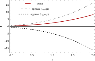
Figure 1: The behavior of the extra term $\mathbb{T}$ as a function of the redshift $z$ for the new exact expression (solid curve), and for the previously considered approximate relations, for $L_{m}=-\rho$ (dashed curve), and $L_{m}=P$ (dotted curve), respectively.

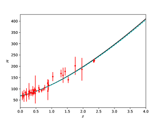
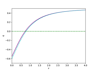
Figure 2: The behavior of the Hubble parameter $H$ and of the deceleration parameter $q$ as a function of the redshift for the best fit values of the parameters as given by Eqs. (IV). The dashed line represents the $\Lambda$CDM model.

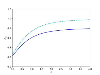
Figure 3: The behavior of the matter density parameter $\Omega_{m}$ as a function of redshift for the best fit values of the parameters as given by Eq. (IV). The dashed line represents the $\Lambda$CDM model.

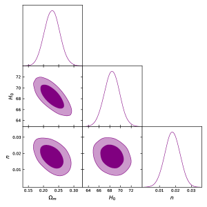
Figure 4: The corner plot for the values of the parameters $H_{0}$, $\Omega_{m0}$ and $n$ with their $1\sigma$ and $2\sigma$ confidence levels.

With the use of the mathematical identity

$$\left(\square\nabla_{\nu}-\nabla_{\nu}\square\right)f_{R}=R_{\mu\nu}\nabla^{\mu}f_{R},$$

after taking the divergence of Eq. (IV) we obtain the conservation equation in the $f\left(R,T\right)$ gravity theory in the form

$$\left(\frac{1}{2}-f_{T}\right)\nabla^{\mu}T_{\mu\nu} =\left(T_{\mu\nu}+\mathbb{T}_{\mu\nu}\right)\nabla^{\mu}f_{T}$$

$$+f_{T}\left(\nabla^{\mu}\mathbb{T}_{\mu\nu}+\frac{1}{2}\nabla_{\nu}T\right).$$ (56)

As one can see from the field equations (IV), the dynamical behavior in $f(R,T)$ gravity essentially depends on the tensor $\mathbb{T}_{\mu\nu}$. In this Letter, we will consider a simple case that indicates the importance of the new term. Let us assume that $f(R,T)=\alpha|T|^{n}$, and $P=0$. In this case, the field equations reduce to

$$\kappa^{2}G_{\mu\nu}=\frac{1}{2}T_{\mu\nu}+\frac{1}{2}\alpha|T|^{n}g_{\mu\nu}-n\alpha\epsilon|T|^{n-1}(T_{\mu\nu}+\mathbb{T}_{\mu\nu}),$$ (57)

where $\epsilon=sign(T)$. Here we have $T=-\rho$ and then $\epsilon=-1$. The Friedmann and Raychaudhuri equations are then

$$h^{2} =\bar{\rho}_{m}-\beta(3n+1)\bar{\rho}_{m}^{n},$$ (58)

$$h^{\prime} =-\frac{3}{2}\left(\bar{\rho}_{m}-4\beta n\bar{\rho}_{m}^{n}\right),$$ (59)

where we have used the following set of dimensionless variables,

$$\tau =H_{0}t,\quad H=H_{0}h,$$

$$\bar{\rho} =\frac{\rho}{6\kappa^{2}H_{0}^{2}},\quad\beta=(6\kappa^{2}H_{0}^{2})^{n-1}\alpha,$$ (60)

and we have denoted by $H_{0}$ the current value of the Hubble parameter, and by a prime the derivative with respect to $\tau$. As an indicator of the decelerating/accelerating evolution we introduce the deceleration parameter, defined as

$$q=\frac{d}{d\tau}\frac{1}{h}-1.$$ (61)

Note that from the normalized Friedmann equation (58), and by taking into account that at the present time we have $h(present)=1$, we can obtain the coupling $\beta$ as

$$\beta=-\frac{1-\Omega_{m0}}{(1+3n)\Omega_{m0}^{n}}.$$ (62)

In order to find the best fit value of the parameter $n$, $H_{0}$ and $\Omega_{m0}$, we use the Likelihood analysis using the observational data on the Hubble parameter in the redshift range $z\in(0.07,2.36)$ [27]. In the case of independent data points, the likelihood function can be defined as

$$L=L_{0}e^{-\chi^{2}/2},$$ (63)

where $L_{0}$ is the normalization constant and the quantity $\chi^{2}$ is defined as

$$\chi^{2}=\sum_{i}\left(\frac{O_{i}-T_{i}}{\sigma_{i}}\right)^{2}.$$ (64)

Here $i$ counts the data points, $O_{i}$ are the observational value, $T_{i}$ are the theoretical values, and $\sigma_{i}$ are the errors associated with the $i$th data obtained from observations.

By maximizing the likelihood function, the best fit values of the parameters $n$, $\Omega_{m0}$ and $H_{0}$ at $1\sigma$ confidence level, can be obtained as

$$\Omega_{m0} =0.228^{+0.025}_{-0.025},$$

$$H_{0} =68.396^{+1.421}_{-1.437},$$

$$n =0.018^{+0.005}_{-0.005}.$$ (65)

Also, with the use of equation (62) we obtain

$$\beta=-0.756^{+0.031}_{-0.030}.$$ (66)

The redshift evolution of the Hubble function, of the deceleration parameter $q$, and of the matter density parameter $\Omega_{m}=\bar{\rho}_{m}/h^{2}$ are represented, for this model, in Figs. 2 and 3, respectively. Also, the corner plot for the values of the parameters $H_{0}$, $\Omega_{m0}$ and $n$ with their $1\sigma$ and $2\sigma$ confidence levels is shown in Fig. 4.

V Discussions and final remarks

In the present Letter we have obtained the complete expression of the first variation of the matter energy-momentum tensor with respect to the metric $g^{\mu\nu}$, and of its associated tensor $\mathbb{T}_{\mu\nu}$. The full estimation of this term requires the calculation of the second variations of the matter Lagrangian with respect to the metric, a term which was generally ignored in the previous investigations of this problem. The expression of $\delta^{2}L_{m}/\delta g^{\mu\nu}\delta g^{\alpha\beta}$ can be calculated straightforwardly from the first variation $\delta L_{m}/\delta g^{\mu\nu}$, which can be obtained for the two possible choices of the matter Lagrangian either from thermodynamic considerations, or in a direct way by using the definition of the energy-momentum tensor. The main result of this Letter is that the first variation of the matter energy-momentum tensor, given by Eq. (III), is independent of the choice of the matter Lagrangian; both possible choices lead to the same expression (III), depending only on the thermodynamic pressure, and its second variation. The variation of the energy-momentum tensor can also be expressed in terms of the pressure, and the energy-momentum tensor itself, or in a compact form in terms of a generalized energy-momentum tensor, formally defined in Eq. (40).

The new form of the variation of the matter energy-momentum tensor may have some important implications on modified gravity theories with geometry-matter coupling. As an important example we have considered the particular case of the $f(R,T)$ gravity theory. We have investigated the cosmological implications of a particular representation of the $f(R,T)$ gravity, with action given by Eq. (54), in which the standard Hilbert-Einstein Lagrangian is replaced by a general term $f(R,T)$. As a simple case we have taken $f(R,T)=\alpha|T|^{n}$. The generalized Friedmann equations take a simple form, and they allow a complete analysis of the cosmological features of this simple model, and a full fitting of the observational cosmological data, which permits the determination of the optimal values of the free parameters. The model gives an excellent description of the observational data for the Hubble function, up to a redshift of $z\approx 4$. In this redshift range the model basically coincides with the $\Lambda$CDM model. The transition from acceleration to deceleration takes place a redshift that again coincides with the $\Lambda$CDM value. Moreover, the deceleration parameter $q$ basically coincides with the $\Lambda$CDM prediction. However, significant differences in the behavior of the matter density do appear at higher redshifts.

The search for the “true” physical quantities from which the matter energy-momentum tensor can be obtained ($-\rho$ or $P$) in a variational formulation is still going on. Interestingly enough, the two possible matter Lagrangians are not equivalent in any sense (physical or mathematical), but their functional variation coincides, leading to the same energy-momentum tensor. However, as shown in the present Letter, the first variation of the matter energy-momentum tensor is independent on the adopted form of the matter Lagrangian, making the modified gravity theories containing this term unique, and well defined. Hence, the study of the various orders of variations of the matter Lagrangians and of the energy-momentum tensor turns out to be an important field of research, which could lead to a new understanding of the mathematical formalism, and of the astrophysical and cosmological implications of the modified gravitational theories, and in particular of the $f(R,T)$ gravity.

References

- [1] T. Harko and F. S. N. Lobo, Int. J. Mod. Phys. D 29, 2030008 (2020).
- [2] D. H. Weinberg, M. J. Mortonson, D. J. Eisenstein, C. Hirata, A. G. Riess, and E. Rozo, Physics Reports 530, 87 (2013).
- [3] D. Brout et al., Astrophys. J. 938, 110 (2022).
- [4] N. Aghanim et al., Planck 2018 results. VI. Cosmological parameters, Astron. Astrophys. 641, A6 (2020).
- [5] S. Tsujikawa, Class. Quant. Grav. 30, 214003 (2013).
- [6] J. de Haro and L. A. Saló, Galaxies 9, 73 (2021).
- [7] S. Nojiri, S. D. Odintsov, and V. K. Oikonomou, Phys. Rept. 692, 1 (2017).
- [8] J. B. Jimenez, L. Heisenberg, and T. Koivisto, Phys. Rev. D 98, 044048 (2018).
- [9] T. Harko, T. S. Koivisto, F. S. N. Lobo and G. J. Olmo, Phys. Rev. D 85, 084016 (2012).
- [10] Z. Haghani, T. Harko, H. R. Sepangi, and S. Shahidi, JCAP 10, 061 (2012).
- [11] R. Hama, T. Harko, S. V.. Sabau, and S. Shahidi, Eur. Phys. J. C 81, 742 (2021).
- [12] R. Hama, T. Harko, and S. V. Sabau, Eur. Phys. J. C 82, 385 (2022).
- [13] O. Bertolami, C. G. Boehmer, T. Harko, and F. S. N. Lobo, Phys. Rev. D 75, 104016 (2007).
- [14] T. Harko and F. S. N. Lobo, Eur. Phys. J. C 70, :373 (2010).
- [15] T. Harko, F. S. N. Lobo, S. Nojiri, and S. D. Odintsov, Phys. Rev. D 84, 024020 (2011).
- [16] Z. Haghani, T. Harko, F. S. N. Lobo, H. R. Sepangi, and S. Shahidi, Phys. Rev. D 88, 044023 (2013).
- [17] T. Harko, F. S. N. Lobo, G. Otalora, and E. N. Saridakis, Phys. Rev. D 89, 124036 (2014).
- [18] Y. Xu, G. Li, T. Harko, and S.-D. Liang, Eur. Phys. J. C 79, 708 (2019).
- [19] T. Harko, N. Myrzakulov, R. Myrzakulov, and S. Shahidi, PDU 34, 100886 (2021).
- [20] T. Harko and F. S. N. Lobo, Extensions of gravity: Curvature-Matter Couplings and Hybrid Metric-Palatini Theory, Cambridge University Press, Cambridge, 2018
- [21] T. P. Sotiriou and V. Faraoni, Class. Quant. Grav. 25, 205002 (2008).
- [22] O. Bertolami, F. S. N. Lobo and J. Paramos, Phys. Rev. D 78, 064036 (2008).
- [23] T. Harko, Phys. Rev. D 81, 044021 (2010).
- [24] O. Minazzoli and T. Harko, Phys. Rev. D 86, 087502 (2012).
- [25] J. D. Brown, Class. Quant. Grav. 10, 1579 (1993).
- [26] F. de Felice and C. J. S. Clarke, Relativity on curved manifolds, Cambridge University Press, Cambridge, 1990
- [27] O. Farooq, et. al, Astophys. J. 835, 26 (2017).