Constraints on the Parameterized Deceleration Parameter in FLRW Universe

Abstract

Confirmation of accelerated expansion of the universe probed the concept of dark energy theory, and since then, numerous models have been introduced to explain its origin and nature. The present work is based on reconstructing dark energy by parametrization of the deceleration parameter in the FLRW universe filled with radiation, dark matter and dark energy. We have chosen some well-motivated parametrized models 1-3 in an attempt to investigate the energy density in terms of deceleration parameters by estimating the cosmological parameters with the help of different observational datasets. Also, we have introduced a new model 4 for the parametrization of the deceleration parameter. Then we analyzed the cosmography parameters using the best-fit values of the parameters. Using the information criteria, we have examined the viability of the models.

I Introduction

The concept of cosmic acceleration was probably one of the most promising discoveries in the modern cosmology paradigm. Recently, two independent research works involving distant supernovae suggested that in the present epoch, the universe is undergoing an accelerated expansion [1, 2]. This phenomenon has been favorably explained later by the existence of an energy component with massive negative pressure comprising nearly 70% of the universe. This is known as “dark energy” (DE). The nature of this is still unidentified. Synchronizing with the observed data, many DE models have been proposed so far. Among them, the $\Lambda$CDM model is widely accepted as supposedly it ‘best accommodates’ the observations but also it comes with some disadvantages like a fine-tuning problem, coincidence problems, and so on [3, 4, 5]. To overcome these drawbacks, alternative DE models have been explored like a quite favorable phantom, $k$-essence, Chaplygin gas, etc, [6] for possible explanations of the origin and nature of the dark energy. However, prior to the accelerated phase, the universe had gone through a decelerated phase in the early epoch where the effects of dark energy were absent or subdominant, some recent late-time cosmic acceleration is discussed in [7, 8, 9, 10]. It is believed that density perturbations occurred in this epoch which played a key role in the structural formation of the universe. So, to cover the entire evolution, we would have to employ a cosmological model which would simultaneously describe the accelerated and decelerated phases. Earlier, the definition of cosmology was addressed by Sandage[11] as a search for two simple but fundamental cosmographic parameters: Hubble parameter ($H_{0}$), which determined the expansion rate and a small correction $q_{0}$ due to gravity, known as deceleration parameter (DP), responsible for slowing down the expansion. Though the inclusion of ‘dark energy has completely changed the scenario, but still, any practical aspect of cosmological evolution is tightly bound to DP. It is defined as $q=-\frac{a\ddot{a}}{\dot{a}^{2}}$ where $a(t)$ is the scale factor of the universe. $q>0$ ($\ddot{a}<0$) indicates a decelerating universe and vice versa. While HP describes the linear part of the time dependence of the scale factor, the non-linear correction term $q_{0}$ opens up possibilities like the presence of local instabilities or the existence of chaotic regimes [12]. Moreover, the dynamics of observable galaxy number variation can be determined through DP. Like DE cosmological models, DE has been subjected to numerous modifications to be better fitted with observational data.

Parametrization of DP as a function of scale factor $a$ or redshift $z$ can be accounted as a suitable approach to it. Limitations to such parametric assumptions are: (i) Most of the parametrizations diverge in the distant future and some of them are only valid at low redshift limit ($z<<1$) [13, 14]; (ii) Prior parametric assumptions may be in conflict with the true nature of the dark energy. (iii) In non-parametric models, evolution can be directly deduced from observational data avoiding parametric assumptions [15, 16, 17, 18, 19]. However, it can help to improve the efficiency of future cosmological surveys. So in pursuit of understanding the transition from decelerated to accelerated phase, the parametrization approach can be proved fruitful. Recently Capozziello reconstructed a divergence-free form of DP starting with Pade polynomials and analyzed the corresponding observational data [20]. A logarithmic parametrization of DP was proposed in ref. [21], and the constraints were obtained by using type Ia supernova, BAO, and CMB data sets. Motivated by these ideas, we have adopted some well-motivated parametrizations of DP to reconstruct dark energy and, consequently, Hubble parameter $H(z)$ in terms of redshift $z$. Mainly, well-established parametrized models have been introduced for dark energy equation of state and constrain the model parameters by observational data analysis. In the study of the generalized holographic dark energy model, some well-known parametrization type models have been considered [22, 23]. Till now, some authors have assumed some possible forms of parametrization of deceleration parameter [24, 25, 26, 27, 28, 29, 30, 31, 32]. The main advantage behind introducing aparameterized deceleration parameter is to provide a framework that is independent of specific gravitational theories. By parameterizing the deceleration parameter, we can explore the behavior of cosmic expansion without being tied to a particular model. This flexibility allows us to investigate a wide range of cosmological scenarios and potentially uncover new physics beyond our current understanding. Furthermore, in the well-established cosmological models, such as the $\Lambda$CDM model, the focus has primarily been on parameterizing the equation of state of dark energy. However, in the referenced papers [33, 34], the authors have recognized the importance of considering the deceleration parameter as a viable alternative. This motivates us to extend the analysis to include the parametrization of the deceleration parameter for these well-established models and constrains the model parameters by employing MCMC data analysis, which is a powerful statistical technique widely used in cosmology. This approach enables us to explore the parameter space efficiently and extract robust constraints by comparing the theoretical predictions of the models with observational data. Our utilization of MCMC analysis adds a robust statistical framework to our study, enhancing the reliability of our results. A key contribution of our work is the comprehensive comparison of different models with the standard $\Lambda$CDM model. The $\Lambda$CDM model has been highly successful in explaining various cosmological observations, and serves as the benchmark against which we assess the viability of alternative models. By quantitatively evaluating the goodness-of-fit and model selection criteria, we can determine which models provide a better description of the observational data, thereby highlighting their relative viability.

The main focus of the work is to constrain the model parameters using recently released data. Here, in particular, we have chosen to use the updated astronomical datasets: the measurements of Hubble parameter from the differential evolution of cosmic chronometers (CC); SNIa datasets from Type Ia Supernovae sample comprising 1048 measurements; 17 measurements of baryons acoustic oscillation (BAO) data. New constraints on DP have been provided by jointly analyzing the above datasets and implementing Monte Carlo Markov Chain (MCMC) method. The era of modern cosmology promotes the study of kinematic quantities, vastly known as ”Cosmography” or ”Cosmo-kinetics”. The very idea of it is observationally driven and completely independent of any prior assumption of the gravity theory or elected cosmological model. Cosmography presents itself with a compelling advantage as it simply follows the symmetry principles and direct observation- without involving Einstein’s equations (Friedmann equations). Consequently, we can steadfastly avoid some arguable speculations regarding ’dark energy’, ’dark matter’, and others. While pure cosmography does not envision the scale factor $a(t)$ itself but the history of its evolution can be inferred to some extent. Dunajski and Gibbons [35] have studied the constraints on the cosmographic parameters like the deceleration, jerk, and snap parameters for different dark energy models. The parameterization of these quantities is discussed in [36, 37, 38, 39]. Shafieloo, Kim and Linder [26] have discussed the non-parametric reconstruction of these quantities.

The organization of the paper is as follows: In section II, we consider the basic equations of the FLRW model. The Hubble parameter is written in terms of the deceleration parameter. We consider parametrized deceleration parameter models like models 1, 2, 3, and 4. In section III, Section IV deals with the data descriptions like cosmic chronometric datasets, SNIa datasets, and BAO datasets with MCMC results. In section V we fit the models with $H(z)$ and SNIa datasets. In section VI, we discuss the cosmography parameters. In section VII, we analyze the detailed description of the model parameters. In section VIII, we present the information criteria for our models. Finally, the results are presented in section IX.

II Basic Equations of FLRW Model

We have considered a spatially flat, homogeneous, isotropic FLRW the universe with line element

$$ds^{2}=-dt^{2}+a^{2}(t)\left[dr^{2}+r^{2}\left(d\theta^{2}+sin^{2}\theta d\phi^{2}\right)\right]$$ (1)

$a(t)$ being the scale factor.

The energy-momentum tensor of the fluid reads as

$$T_{\mu\nu}=(\rho+p)u_{\mu}u_{\nu}+pg_{\mu\nu}$$ (2)

where $\rho$ and $p$ are the energy density and pressure density of the fluid respectively. The fluid 4-velocity $u^{\mu}=\frac{dx^{\mu}}{ds}$ satisfies the relation $u^{\mu}u_{\mu}=-1$.

For the FLRW Universe, the Friedmann equations in Einstein’s gravity are given by

$$H^{2}=\frac{8\pi G}{3}~{}\rho$$ (3)

and

$$\dot{H}=-4\pi G(\rho+p)$$ (4)

where, $H=\dot{a}/a$ is the Hubble parameter and overhead dot denotes derivative with cosmic time $t$. Considering that the the universe is filled with fluid matter of total energy density $\rho$ and total pressure $p$, it obeys the energy conservation equation

$$\dot{\rho}+3H(\rho+p)=0$$ (5)

We start with the prediction that the universe is composed of matter content comprising radiation, dark matter (DM) and dark energy (DE). So, $\rho$ and $p$ consist of densities and pressures of radiation, DM and DE. So $\rho=\rho_{r}+\rho_{m}+\rho_{d}$ and $p=p_{r}+p_{m}+p_{d}$. Now assume that radiation, DM and DE follows the conservation equation separately so that

$$\dot{\rho}_{r}+3H(\rho_{r}+p_{r})=0,$$ (6)

$$\dot{\rho}_{m}+3H(\rho_{m}+p_{m})=0$$ (7)

and

$$\dot{\rho}_{d}+3H(\rho_{d}+p_{d})=0$$ (8)

For radiation, $p_{r}=\frac{1}{3}\rho_{r}$, so from equation (6) we obtain $\rho_{r}=\rho_{r0}a^{-4}$. Since the DM follows negligible pressure (i.e., $p_{m}=0$), so from equation (7) we obtain $\rho_{m}=\rho_{m0}a^{-3}$.

Let us consider the deceleration parameter

$$q=-1-\frac{\dot{H}}{H^{2}}$$ (9)

The corresponding deceleration parameter for DE is given by

$$q_{d}=-1-\frac{\dot{H_{d}}}{H_{d}^{2}}$$ (10)

where $H_{d}$ is the Hubble expansion rate of the dark energy term. So from equations (3) and (4), we can write

$$H_{d}^{2}=\frac{8\pi G}{3}~{}\rho_{d}$$ (11)

and

$$\dot{H}_{d}=-4\pi G(\rho_{d}+p_{d})$$ (12)

Using the field equations (11) and (12) and the energy-conservation equation (8), the fluid energy density becomes

$$\rho_{d}=\rho_{d0}~{}e^{\int\frac{2(1+q_{d})}{1+z}dz}$$ (13)

where $\rho_{d0}$ represents the present value of the density parameter and $z$ is the redshift parameter described as $1+z=\frac{1}{a}$ (presently, $a_{0}=1$). Defining $\Omega_{r0}=\frac{8\pi G\rho_{r0}}{3H_{0}^{2}}$, $\Omega_{m0}=\frac{8\pi G\rho_{m0}}{3H_{0}^{2}}$ and $\Omega_{d0}=\frac{8\pi G\rho_{d0}}{3H_{0}^{2}}$, from equation (3), we obtain the Hubble parameter as

$$H^{2}(z)=H_{0}^{2}\left[\Omega_{r0}(1+z)^{4}+\Omega_{m0}(1+z)^{3}+\Omega_{d0}~{}e^{\int\frac{2(1+q_{d})}{1+z}dz}\right]$$ (14)

where $\Omega_{d0}=1-\Omega_{r0}-\Omega_{m0}$.

To find the deceleration parameter $q$ using the expression for the Hubble parameter $H(z)$, we first need to calculate the derivative of $H(z)$ with respect to $z$. Then we substitute this derivative into the formula for $q$. Differentiating both sides of the equation with respect to $z$, we have:

$$2H(z)\frac{dH(z)}{dz} =H_{0}^{2}\left[4\Omega_{r0}(1+z)^{3}+3\Omega_{m0}(1+z)^{2}\right.$$ (15)

$$\quad+\left.\frac{2(1+q_{d})\Omega_{d0}}{(1+z)}e^{\int\frac{2(1+q_{d})}{1+z}dz}\right]$$

Now, we can substitute this derivative of $H(z)$ into the expression for $q$:

$$q=-1-\frac{\dot{H}}{H^{2}}=-1-\frac{2H(z)\frac{dH(z)}{dz}}{H(z)^{2}}$$ (16)

Substituting the expression for $\frac{dH(z)}{dz}$ derived earlier, we get:

$$q=-1-\frac{2}{H(z)}\bigg{[} 4\Omega_{r0}(1+z)^{3}+3\Omega_{m0}(1+z)^{2}$$ (17)

$$+\frac{2(1+q_{d})\Omega_{d0}}{(1+z)}e^{\int\frac{2(1+q_{d})}{1+z}dz}\bigg{]}$$

Now, one could evaluate $H(z)$ using the given values of $\Omega_{r0}$, $\Omega_{m0}$, $\Omega_{d0}$, and $q_{d}$ at the specific redshift $z$ you are interested in, and substitute it into the equation to calculate the corresponding deceleration parameter $q$.

For $\Lambda$CDM model, by adding the cosmological constant $\Lambda$ terms in equations (3) and (4) and by assuming the density parameter $\Omega_{\Lambda 0}=\frac{\Lambda}{3H_{0}^{2}}$, the deceleration parameter $q$ from equation (9) can be written as

$$q(z)=\frac{\left[2\Omega_{r0}(1+z)^{4}+\Omega_{m0}(1+z)^{3}-2\Omega_{\Lambda 0}\right]}{2\left[\Omega_{r0}(1+z)^{4}+\Omega_{m0}(1+z)^{3}+\Omega_{\Lambda 0}\right]}$$ (18)

where $\Omega_{\Lambda 0}=1-\Omega_{r0}-\Omega_{m0}$. The present value of the deceleration parameter is found by inserting $z=0$, which gives $q(z=0)=\frac{\left[2\Omega_{r0}+\Omega_{m0}-2\Omega_{\Lambda 0}\right]}{2\left[\Omega_{r0}+\Omega_{m0}+\Omega_{\Lambda 0}\right]}~{}.$

III Parameterized deceleration parameter

Most simplest parametrization of $q$ which contains two parameters can be taken as

$$q(z)=q_{0}+q_{1}\mathcal{X}(z)$$ (19)

where $q_{0}$ and $q_{1}$ are constants and $\mathcal{X}(z)$ is a function of redshift $z$. In search of satisfactory solutions to the cosmological puzzles, many forms of $\mathcal{X}(z)$ has been suggested. As mentioned earlier, most of them were inadequate in explaining future evolution scenarios. So the persuasion of an ideal divergence-free parametrization of DP is still relevant. The well-known parametrized equation of state parameter models has been introduced by several authors, and the corresponding analogous of these models for parametrized deceleration parameters have been introduced in [33, 34]. Here, we have adopted the analogous of some well-known parametrized models for the deceleration parameter, which contains two unknown parameters and calculated the corresponding Hubble parameter in terms of redshift $z$.

III.1 Model 1 (Wetterich type)

The Wetterich model for the parametrized equation of state parameter has been studied in [40, 41]. The analogous Wetterich type parametrization of the deceleration parameter has been introduced in [33, 34] and is given by

$$q_{d}(z)=\frac{q_{0}}{1+q_{1}1og(1+z)}$$ (20)

where $q_{0}$ and $q_{1}$ are constants. Then the energy density will be given by

$$\rho_{d}=\rho_{d0}~{}(1+z)^{2}~{}\left\{1+q_{1}~{}log(1+z)\right\}^{\frac{2q_{0}}{q_{1}}}$$ (21)

From equation (14), we obtain

$$H^{2}(z) =H_{0}^{2}\left[\Omega_{r0}(1+z)^{4}+\Omega_{m0}(1+z)^{3}\right.$$ (22)

$$\left.+\left(1-\Omega_{r0}-\Omega_{m0}\right)(1+z)^{2}\left\{1+q_{1}\log(1+z)\right\}^{\frac{2q_{0}}{q1}}\right]$$

III.2 Model 2 (Barboza-Alcaniz type)

The Barboza-Alcaniz model for parametrized equation of state parameter has been studied in [42]. The analogous Barboza-Alcaniz type parametrization of deceleration parameter has been introduced in [33, 34] and is given by

$$q_{d}(z)=q_{0}+q_{1}\frac{z(1+z)}{1+z^{2}}$$ (23)

where $q_{0}$ and $q_{1}$ are constants. Then the energy density will be

$$\rho_{d}=\rho_{d0}~{}(1+z)^{2(1+q_{0})}~{}\left(1+z^{2}\right)^{q_{1}}$$ (24)

From equation (14), we obtain

$$H^{2}(z) =H_{0}^{2}\left[\Omega_{r0}(1+z)^{4}+\Omega_{m0}(1+z)^{3}\right.$$ (25)

$$\left.+\left(1-\Omega_{r0}-\Omega_{m0}\right)(1+z)^{2(1+q_{0})}~{}\left(1+z^{2}\right)^{q_{1}}\right]$$

III.3 Model 3 (CPL type)

The famous Chevallier-Polarski-Linder (CPL) model for parametrized equation of state parameter has been studied in [36, 37]. The analogous CPL type parametrization of deceleration parameter has been introduced in [33, 34] and is given by

$$q_{d}(z)=q_{0}+q_{1}\frac{z}{1+z}$$ (26)

where $q_{0}$ and $q_{1}$ are constants. Subsequently, the energy density (13) becomes

$$\rho_{d}=\rho_{d0}~{}(1+z)^{2(1+q_{0}+q_{1})}~{}e^{\frac{2q_{1}}{1+z}}$$ (27)

From equation (14), we obtain

$$H^{2}(z) =H_{0}^{2}\left[\Omega_{r0}(1+z)^{4}+\Omega_{m0}(1+z)^{3}\right.$$ (28)

$$\left.+\left(1-\Omega_{r0}-\Omega_{m0}\right)(1+z)^{2(1+q_{0}+q_{1})}~{}e^{\frac{2q_{1}}{1+z}}\right]$$

III.4 Model 4

Here we propose a new parametrized model for deceleration parameter and is given as in the form:

$$q_{d}(z)=q_{0}+q_{1}\frac{1+z}{2+z}$$ (29)

where $q_{0}$ and $q_{1}$ are constants. Subsequently, the energy density (13) becomes

$$\rho_{d}=\rho_{d0}~{}(1+z)^{2(1+q_{0})}(2+z)^{2q_{1}}$$ (30)

From equation (14), we obtain

$$H^{2}(z) =H_{0}^{2}\left[\Omega_{r0}(1+z)^{4}+\Omega_{m0}(1+z)^{3}\right.$$ (31)

$$\left.+\left(1-\Omega_{r0}-\Omega_{m0}\right)(1+z)^{2(1+q_{0})}(2+z)^{2q_{1}}\right]$$

IV Data Analysis

In this section, we will constrain our model parameters by using three types of dataset. The CC datasets consist 31 measurements, The SNIa dataset consists 1048 measurements and 17 measurements of BAO to obtain the best-fit value of our model parameters. We have implemented the Markov Chain Monte Carlo (MCMC) [43] and implemented with the open-source package Polychord [44] and GetDist [45]. The total $\chi^{2}$ function of the combination CC + BAO + SNIa and define as

$$\chi^{2}=\chi_{CC}^{2}+\chi_{SNIa}^{2}+\chi_{BAO}^{2}.$$

IV.1 Data description

IV.1.1 Cosmic Chronometric (CC) datasets

We consider the compilation of 31 measurements of CC lying between the redshift range $0.07\leq z\leq 1.965$. The underlying principle for these measurements was proposed in [46], by relating the Hubble parameter with redshift $z$, and cosmic time $t$

$$H(z)=-\frac{1}{1+z}\frac{\mathrm{d}z}{\mathrm{~{}d}t}$$

The $\chi^{2}$ function for these measurements, denoted by

$\chi_{\mathrm{CC}}^{2}$, is

$$\chi_{\mathrm{CC}}^{2}=\sum_{i=1}^{31}\frac{\left[H^{th}\left(z_{i}\right)-H^{obs}\left(z_{i}\right)\right]^{2}}{\sigma_{H^{\mathrm{obs}}\left(z_{i}\right)}^{2}},$$ (32)

where $H^{\mathrm{th}}\left(z_{i},k,\alpha,h\right)$ represent the theoretical value obtained from our cosmological model, $H^{\text{obs }}\left(z_{i}\right)$ and represent the observed value of hubble parameter with standard deviation $\sigma_{H^{\mathrm{obs}}\left(z_{i}\right)}^{2}$. (to see more and rundown all measurements see [47])

IV.1.2 type Ia supernova (SNIa) datasets

The 1048 measurements of type Ia supernovae from five different sub-samples SNLS, SDSS, PSI, low-$z$, and HST in the redshift range of $0.01<z<2.3$ [48]. The $\chi^{2}$ function of the SNIa data is given as

$$\chi_{\mathrm{SNIa}}^{2}=\Delta\mu C_{\mathrm{Pan}}^{-1}\Delta\mu^{T},$$ (33)

where $\Delta\mu=\mu_{i}^{\text{obs }}-\mu^{\text{th }}$. Where $\left(\mu_{i}^{\text{obs }}\right)$ represented as observed distance modulus and evaluated as

$$\mu_{i}^{\text{obs }}=\mu_{B,i}+\mathcal{M},$$ (34)

$\mu_{B,i}$ represents the observed peak magnitude at maximum in the rest frame of the $B$ band for redshift $z_{i}$, while $\mathcal{M}$ represents nuisance parameter. The theoretical distance modulus was evaluated as

$$\mu^{\text{th }}=5\log_{10}D_{L}+\mathcal{M},$$ (35)

where

$$D_{L}=\left(1+z_{\mathrm{hel}}\right)\int_{0}^{z_{\mathrm{cmb}}}\frac{H_{0}dz}{H(z)},$$ (36)

with $z_{\text{hel }}$ is heliocentric and $z_{\mathrm{cmb}}$ is CMB rest frame redshifts. The covariance matrix is measured as $C_{\text{Pan }}=C_{\text{sys }}+D_{\text{stat }}$. Where $C_{\text{sys }}$ is the systematic covariance matrix and $D_{\text{stat }}$ stands for diagonal of the covariance matrix of the statistical uncertainty and is calculated as

$$D_{\text{stat },ii}=\sigma_{\mu_{B,i}}^{2}.$$ (37)

The description and the systematic covariance matrix together with $\mu_{B,i},\sigma_{\mu_{B,i}}^{2},z_{\mathrm{cmb}}$, and $z_{\text{hel }}$ for the $i$ th SnIa are mentioned in [49].

IV.1.3 Baryon Acoustic Oscillations

We picked 17 BAO [50] measurements from the greatest collection of BAO dataset of (333) measurements since adopting the entire catalog of BAO might lead in a very significant error owing to data correlations, therefore we opted for a small dataset to minimize inaccuracies. Transverse BAO studies contribute measurements of $D_{H}(z)/r_{d}=c/H(z)r_{d}$ with comoving angular diameter distance.[51] [52].

$$D_{M}=\frac{c}{H_{0}}S_{k}\left(\int_{0}^{z}\frac{dz^{\prime}}{E\left(z^{\prime}\right)}\right)\text{, }$$ (38)

where

$$S_{k}(x)=\begin{cases}\frac{1}{\sqrt{\Omega_{k}}}\sinh\left(\sqrt{\Omega_{k}}x\right)&\text{ if }\quad\Omega_{k}>0\\ x&\text{ if }\quad\Omega_{k}=0\\ \frac{1}{\sqrt{-\Omega_{k}}}\sin\left(\sqrt{-\Omega_{k}}x\right)&\text{ if }\quad\Omega_{k}<0.\end{cases}$$ (39)

We also consider the angular diameter distance $D_{A}=$ $D_{M}/(1+z)$ and the $D_{V}(z)/r_{d}$. which is combination of the BAO peak coordinates and $r_{d}$ is the sound horizon at the drag epoch. Finally we can obtain ”line-of-sight” (or ”radial”) observations directly the Hubble parameter

$$D_{V}(z)\equiv\left[zD_{H}(z)D_{M}^{2}(z)\right]^{1/3}\text{. }$$ (40)

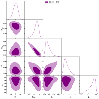
Figure 1: The above figure shows the MCMC confidence contours at 1$\sigma$ and 2$\sigma$ obtained from CC+SNIa+BAO dataset for Model 1 (Wetterich type).

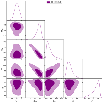
Figure 2: The above figure shows the MCMC confidence contours at 1$\sigma$ and 2$\sigma$ obtained from CC+SNIa+BAO dataset for Model 2 (Barboza-Alcaniz type).

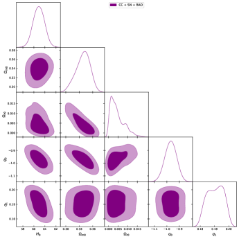
Figure 3: The above figure shows the MCMC confidence contours at 1$\sigma$ and 2$\sigma$ obtained from CC+SNIa+BAO dataset for Model 3 (CPL type).

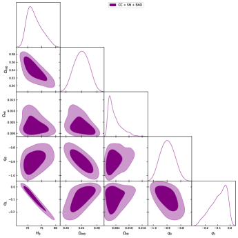
Figure 4: The above figure shows the MCMC confidence contours at 1$\sigma$ and 2$\sigma$ obtained from CC+SNIa+BAO dataset for Model 4.

MCMC Results
Model	Priors	Parameters	Best fit Value
$\Lambda$CDM Model	$[50.,100.]$	$H_{0}$	$69.854848_{-1.259100}^{+1.259100}$
	$[0.,1.]$	$\Omega_{\mathrm{m0}}$	$0.268654_{-0.012822}^{+0.012822}$
	$[0.,1]$	$\Omega_{\Lambda}$	$0.724585_{-0.009373}^{+0.009373}$
Model 1	$[50.,100.]$	$H_{0}$	$68.990853_{-0.502428}^{+0.502428}$
	$[0.,1.]$	$\Omega_{\mathrm{m0}}$	$0.221900_{-0.022982}^{+0.022982}$
	$[0.,1]$	$\Omega_{\mathrm{r0}}$	$0.007835_{-0.005651}^{+0.005651}$
	$[-1.5,-0.5]$	$q_{0}$	$-0.941550_{-0.043352}^{+0.043352}$
	$[0.,1.]$	$q_{1}$	$0.740557_{-0.220903}^{+0.220903}$
Model 2	$[50.,100.]$	$H_{0}$	$69.061167_{-0.498457}^{+0.498457}$
	$[0.,1.]$	$\Omega_{\mathrm{m0}}$	$0.231719_{-0.025169}^{+0.025169}$
	$[0.,1]$	$\Omega_{\mathrm{r0}}$	$0.006670_{-0.005154}^{+0.005154}$
	$[-1.5,-0.5]$	$q_{0}$	$-0.924723_{-0.052163}^{+0.052163}$
	$[0.,1.]$	$q_{1}$	$0.251461_{-0.084597}^{+0.084597}$
Model 3	$[50.,100.]$	$H_{0}$	$60.450021_{-0.511464}^{+0.511464}$
	$[0.,1.]$	$\Omega_{\mathrm{m0}}$	$0.338454_{-0.015533}^{+0.015533}$
	$[0.,1]$	$\Omega_{\mathrm{r0}}$	$0.004485_{-0.003527}^{+0.003527}$
	$[-1.5,-0.5]$	$q_{0}$	$-0.968857_{-0.046034}^{+0.046034}$
	$[0.,1.]$	$q_{1}$	$0.190554_{-0.006576}^{+0.006576}$
Model 4	$[50.,100.]$	$H_{0}$	$71.392060_{-2.608372}^{+2.608372}$
	$[0.,1.]$	$\Omega_{\mathrm{m0}}$	$0.240129_{-0.021352}^{+0.021352}$
	$[0.,1]$	$\Omega_{\mathrm{r0}}$	$0.003402_{-0.002740}^{+0.002740}$
	$[-1.5,-0.5]$	$q_{0}$	$-0.897355_{-0.056271}^{+0.056271}$
	$[-0.5,0.5]$	$q_{1}$	-$0.091362_{-0.073319}^{+0.073319}$

Table 1: Summary of the MCMC results using CC + SNIa + BAO dataset.

V Observational, and theoretical comparisons of the Hubble and Distance Modulus functions

After determining the free parameters of Models 1-4, we can proceed to compare the predictions of these models with observational data. Additionally, we compare the model predictions to the well-established $\Lambda$CDM model, which serves as the base model for comparison. To provide a comprehensive analysis, we also consider the error bands associated with the $\Lambda$CDM model. This comparative analysis allows us to assess the viability and performance of the proposed models in capturing the observed data and to evaluate their agreement with the widely accepted $\Lambda$CDM model, providing insights into the potential strengths and limitations of each model in explaining the observed universe.

V.1 Comparison with the Hubble data points.

First, We consider the comparison of the Models (1 - 4) with the 31 (CC) data points and the $\Lambda$CDM model with 1 $\sigma$ and 2 $\sigma$ error bands . The comparison findings are shown in Figure 5, 8, 8 and 8. The Figure shows that all models fit with (CC) dataset quite well.

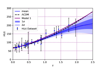
Figure 5: The figure shows that the theoretical curve of the Hubble function $H(z)$ of Model 1 is shown in purple line and $\Lambda$CDM Model shown in black dotted line with $\Omega_{\mathrm{m0}}=$ 0.3 and $\Omega_{\Lambda}=$ 0.7 against 57 $H(z)$ datasets are shown in blue dots with their corresponding error bars with 1$\sigma$ and 2$\sigma$ error bands.

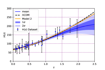
Figure 6: The figure shows that the theoretical curve of the Hubble function $H(z)$ of Model 2 is shown in orange line and $\Lambda$CDM Model shown in black dotted line with $\Omega_{\mathrm{m0}}=$ 0.3 and $\Omega_{\Lambda}=$ 0.7 against 57 $H(z)$ datasets are shown in blue dots with their corresponding error bars with 1$\sigma$ and 2$\sigma$ error bands.

Figure 7: The figure shows that the theoretical curve of the Hubble function $H(z)$ of Model 3 is shown in green line and $\Lambda$CDM Model shown in black dotted line with $\Omega_{\mathrm{m0}}=$ 0.3 and $\Omega_{\Lambda}=$ 0.7 against 57 $H(z)$ datasets are shown in blue dots with their corresponding error bars with 1$\sigma$ and 2$\sigma$ error bands.

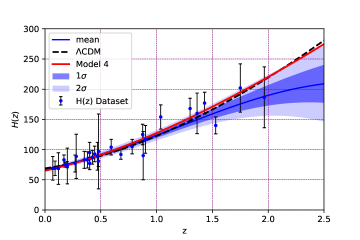
Figure 8: The figure shows that the theoretical curve of the Hubble function $H(z)$ of Model 4 is shown in red line and $\Lambda$CDM Model shown in black dotted line with $\Omega_{\mathrm{m0}}=$ 0.3 and $\Omega_{\Lambda}=$ 0.7 against 57 $H(z)$ datasets are shown in blue dots with their corresponding error bars with 1$\sigma$ and 2$\sigma$ error bands.

V.2 Comparison with the type Ia supernova dataset.

We now compare the $\mu(z)$ distance modulus function of Models (1-4) with the type Ia supernova dataset. From Fig. 10,10,12 and 12 one can see that all Models fit with the type Ia supernova dataset, very well.

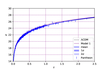
Figure 9: Theoretical curve of distance modulus $\mu(z)$ of the Model 1 is shown in purple line and the $\Lambda$CDM Model is shown in the black dotted line with $\Omega_{\mathrm{m0}}=$ 0.3 and $\Omega_{\Lambda}=$ 0.7 against type Ia supernova data are shown in blue dots with their corresponding errors bars with 1$\sigma$ and 2$\sigma$ error bands.

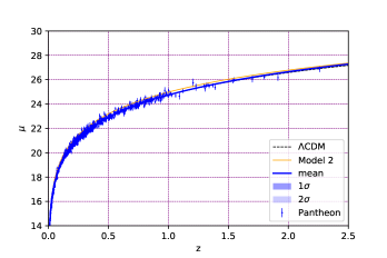
Figure 10: Theoretical curve of distance modulus $\mu(z)$ of the Model 2 is shown in orange line and the $\Lambda$CDM Model is shown in the black dotted line with $\Omega_{\mathrm{m0}}=$ 0.3 and $\Omega_{\Lambda}=$ 0.7, against type Ia supernova data are shown in blue dots with their corresponding errors bars with 1$\sigma$ and 2$\sigma$ error bands.

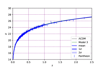
Figure 11: Theoretical curve of distance modulus $\mu(z)$ of the Model 3 is shown in green line and the $\Lambda$CDM Model is shown in the black dotted line with $\Omega_{\mathrm{m0}}=$ 0.3 and $\Omega_{\Lambda}=$ 0.7, against type Ia supernova data are shown in blue dots with their corresponding errors bars with 1$\sigma$ and 2$\sigma$ error bands.

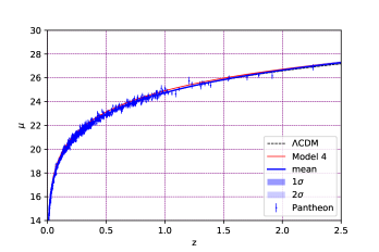
Figure 12: Theoretical curve of distance modulus $\mu(z)$ of the Model 4 is shown in red line and the $\Lambda$CDM Model is shown in the black dotted line with $\Omega_{\mathrm{m0}}=$ 0.3 and $\Omega_{\Lambda}=$ 0.7, against type Ia supernova data are shown in blue dots with their corresponding errors bars with 1$\sigma$ and 2$\sigma$ error bands.

VI Cosmography Parameters

To study the early evolution and late evolution of the universe, some other parameters named cosmographical parameters can be analyzed. The cosmographical parameter like jerk ($j$), snap ($s$) parameters are [53, 54, 55, 56]

$$j=\frac{\dddot{a}}{aH^{3}}=(1+z)\frac{dq}{dz}+q(1+2q),$$ (41)

$$s=\frac{a^{(4)}}{aH^{4}}=-(1+z)\frac{dj}{dz}-j(2+3q)$$ (42)

So the cosmographical parameters contain the higher-order derivatives of the deceleration parameter $q$. The ’jerk’ parameter is considered to have a very useful feature that is for standard $\Lambda$CDM model, $j$ always takes the value unity which helps us assess the deviation regarding different dark energy models. Sahni et al. and Alam et al. analyzed the importance of the jerk parameter $j$ for discriminating various dark energy models. We have explored the evolution of such kinematical quantities with respect to the redshift for the involved parametric models.

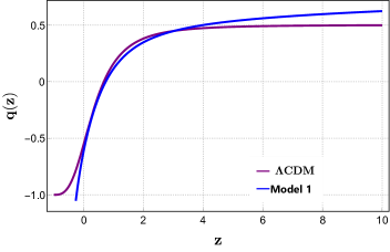
Figure 13: Evolution of deceleration parameter of Model 1 with respect to redshift.

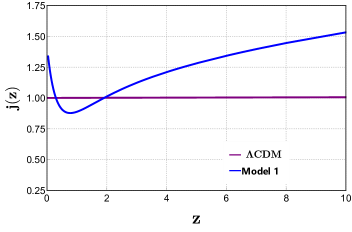
Figure 14: Evolution of jerk parameter of Model 2 with respect to redshift.

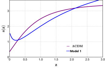
Figure 15: Evolution of snap parameter with of Model 3 with respect to redshift.

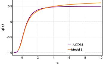
Figure 16: Evolution of deceleration parameter of Model 1 with respect to redshift.

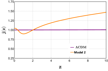
Figure 17: Evolution of jerk parameter of Model 2 with respect to redshift.

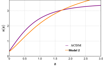
Figure 18: Evolution of snap parameter with of Model 2 with respect to redshift.

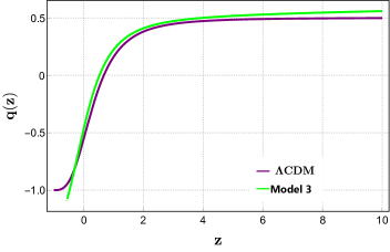
Figure 19: Evolution of decceleration parameter with of Model 3 with respect to redshift.

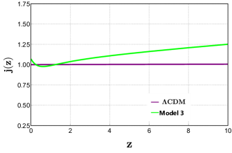
Figure 20: Evolution of jerk parameter of Model 2 with respect to redshift.

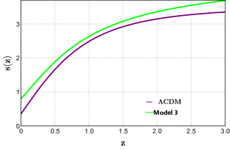
Figure 21: Evolution of snap parameter with of Model 3 with respect to redshift.

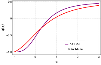
Figure 22: Evolution of deceleration parameter with of Model 4 with respect to redshift.

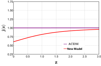
Figure 23: Evolution of jerk parameter with of Model 4 with respect to redshift.

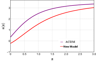
Figure 24: Evolution of snap parameter with of Model 4 respect to redshift.

VII Detailed Description

VII.1 Cosmographic Analysis

The cosmographic analysis provides a universal and effective way to compare the solutions of the theoretical models with cosmological observations. From the observational data, we obtain a set of cosmological parameters, which must be compared with the predicted values of the same parameters obtained from a given model. The result of the comparison allows us to conclude the acceptability of the considered model. Thus, for a complete comparison of all models with the observations and the $\Lambda$CDM model, we will consider an extended set of parameters constructed from the higher-order time derivatives of the scale factor. More exactly, we will concentrate on the comparative behaviour of the deceleration, jerk, and snap parameters of all models and $\Lambda$CDM models.

VII.1.1 Deceleration parameter

While analyzing Model 1’s trajectory, the behavior of the model’s deceleration parameter is nearly comparable to the $\Lambda$CDM model in the redshift range of q $\in$ [-0,2], but Model 1 endures a super acceleration in the future ( Fig: 13). Model 2 appears to have the same behavior as $\Lambda$CDM in the q $\in$ [-0.8,4], but Model 2 is slower since it achieves the value $-0.83565$ as $z\rightarrow 0$. (Fig: 16). In Model 3, this parameter appears to behave similarly to the $\Lambda$CDM model, in q $\in$ [-0.5,6], before experiencing a super acceleration in the near future as ”q = -1.25464” (Fig: 16). Model 4 behaves differently from the $\Lambda$CDM. but it aquire the same value as $\Lambda$CDM in near future 22).

VII.1.2 The jerk parameter

The jerk parameter of Model 1 basically different from $\Lambda$CDM at high as well as low redshift. However, important Model 1 predicts the higher value of $j=1.357595$ at $z=0$ (Fig: 16), Meanwhile, on the other hand, Model 2 also shows different behaviour at both high and low redshift, and seems to coincide with $\Lambda$CDM at redshift value of $z=2$ and $z=0.342566$, and this model also predicts the higher value of $j=1.134545$ (Fig: 19). Model 3 shows different behavior than the $\Lambda$CDM as at high redshift $z>2$, it having a higher value than the $\Lambda$CDM of $j=1.2657$, but it cuts the trajectory of $\Lambda$CDM, twice at $z=1.5$ and $z=0.3$, finally, at lower redshift, it attains the $j$ value of 1.05417, which is a higher than $\Lambda$CDM (Fig: 22). Although the jerk of Model 4 is inconsistent with $\Lambda$CDM, since it shows different evolution at both high and low redshifts and predicts the lower value of $j=0.608251$ (Fig: 24).

VII.1.3 The snap parameter

This parameter of Model 1 and Model 2 is significantly systematic the difference with $\Lambda$CDM within the whole redshift range, but this parameter of Model 1 monotonically decreases in the redshift range of $z>0.3$ and acquires a sudden increase in ”s” value and predicts the higher value of $j=1.608251$ then $\Lambda$CDM, but Model 2 predicts the same value of $j$ as $\Lambda$CDM,(Fig: 16, 19). Model 3 trajectory shows a proper systematic difference with $\Lambda$CDM and predicts a higher value of ”s” as 0.734546 22 Finally, the snap trajectory of Model 4 is notably non-identical with the $\Lambda$CDM, in the given redshift range and accommodate the “s” value of $-0.222743$ as $z\rightarrow 0$. which is lower than $\Lambda$CDM (Fig: 24).

VIII Information Criteria

To discuss the viable model analysis, we need to know the study of information criteria (IC). The Akaike Information Criteria (AIC) [57] is merely used among all ICs. The AIC is an asymptotically unbiased estimator of Kullback-Leibler information as the AIC is an approximate minimization of the Kullback-Leibler information. The Gaussian estimator for the AIC can be written as [58, 59, 60, 61] $\text{AIC}=-2\ln({\cal L}_{max})+2\kappa+\frac{2\kappa(\kappa+1)}{N-\kappa-1}$ where ${\cal L}_{max}$ is the maximum likelihood function, $\kappa$ is the number of parameters of the models, and $N$ is the number of data points used in the data fit of the models. Since for the models, $N\gg 1$, so for this assumption, the above expression converts to the original AIC like $\text{AIC}=-2\ln({\cal L}_{max})+2\kappa$. If the set of models is given, the deviations of the IC values are reduced to $\triangle\text{AIC}=\text{AIC}_{model}-\text{AIC}_{min}=\triangle\chi^{2}_{min}+2\triangle\kappa$ In the study of data analysis, the more favorable range of $\triangle\text{AIC}$ is $(0,2)$. The low favorable range of $\triangle\text{AIC}$ is $(4,7)$, while $\triangle\text{AIC}>10$ provides less support model.

Model	$\chi_{min}^{2}$	$\chi_{red}^{2}$	$AIC$	$\Delta AIC$
$\Lambda$CDM Model	1102.67	0.981	1106.67	0
Model 1	1103.21	0.961	1109.69	0.54
Model 2	1103.05	0.963	1107.05	0.38
Model 3	1103.85	0.965	1107.85	1.18
Model 4	1103.76	0.972	1109.76	3.09

Table 2: Summary of the ${{\chi}^{2}_{min}}$, ${{\chi}^{2}_{red}}$, $AIC$ and $\Delta AIC$.

IX Discussions and Conclusions

We have assumed the FLRW model of the universe in the presence of radiation, dark matter and dark energy. Instead of considering the well-known parametrized dark energy equation of state, we have considered the analogous form of parametrized deceleration parameter for the dark energy component and found the Hubble parameter in terms of redshift with other model parameters. Here we have assumed Model 1 (Wetterich type), Model 2 (Barboza-Alcaniz type) and Model 3 (CPL type), which contains two unknown parameters. Also, we have introduced a new Model 4 for parametrized deceleration parameters, which also contains two unknown parameters. The model parameters have been constrained for $H(z)$ datasets, SNIa datasets, and BAO datasets by MCMC method. Using the best-fit parameters, we have shown the nature of the deceleration parameter, jerk parameter, and snap parameter. The viability of the models has been studied by the information criteria. We have compared all the models as well as compared with the $\Lambda$CDM model (which is the base model) to get which model is more viable than others. From Table: 2, we observe that Models 1 - 4 are all viable models, but (i) Model 3 is more viable than Model 4, (ii) Model 1 is more viable than Model 3 and (iii) Model 2 is more viable than Model 1 compared to the $\Lambda$CDM model. [62]

Acknowledgement: TR is thankful to IIEST, Shibpur, India for providing Institute fellowship (SRF). G. Mustafa is very thankful to Prof. Gao Xianlong from the Department of Physics, Zhejiang Normal University, for his kind support and help during this research. Further, G. Mustafa acknowledges Grant No. ZC304022919 to support his Postdoctoral Fellowship at Zhejiang Normal University.

BAO name	redshift z	Experiment	Measurement	$\bf{Standarddeviation}$	Ref.
6dFGS	$0.106$	${r_{s}}/{D_{V}}$	$0.336$	$0.015$	[63]
SDSS DR7	$0.15$	${D_{V}}(r_{s,fidd}/r_{s})$	$664$	$25.0$	[64]
SDSS-DR7 + 2dFGRS	$0.275$	${r_{s}}/{D_{V}}$	$0.1390$	$0.0037$	[65]
SDSS-DR11 LOWZ	$0.32$	${D_{V}}(r_{d,fidd}/r_{s})$	$1264$	$25$	[66]
SDSS-III DR8	$0.54$	${D_{A}}/{r_{s}}$	$9.212$	$0.41$	[67]
SDSSIII/ DR9	$0.57$	${D_{V}}/{r_{s}}$	$13.67$	$0.22$	[68]
SDSS-IV DR14	$0.72$	${D_{V}}(r_{s,fidd}/r_{s})$	$2353$	$63$	[69]
DES Year 1	$0.81$	${D_{A}}/{r_{s}}$	$10.75$	$0.43$	[70]
DECals DR8	$0.874$	${D_{A}}(r_{s,fidd}/r_{s})$	$1680$	$109$	[69]
	$0.697$	${D_{V}}(r_{s,fidd}/r_{s})$	$2353$	$63$
eBoss DR16 BAO+RSD	$1.48$	${D_{H}}.{r_{s}}$	$13.23$	$0.47$	[71]
SDSS-IV/DR14	$1.52$	${D_{V}}(r_{s,fidd}/r_{s})$	$3843$	$147.0$	[70]
Boss Lya quasars DR9	$2.3$	$H.{r_{s}}$	$34188$	$1188$	[72]
BOSS DR14 Lya in LyBeta	$2.34$	${D_{H}}.{r_{s}}$	$8.86$	$0.29$	[73]
WiggleZ	$0.44$		$0.0870$	$0.0042$
	$0.6$	${r_{s}}/{D_{V}}$	$0.0672$	$0.0031$	[74]
	$0.73$		$0.0593$	$0.0020$

Table 3: Summary of the Baryon Acoustic Oscillations measurements used in this work.

References

- [1] P. Astier, R. Pain, Observational evidence of the accelerated expansion of the universe, Comptes Rendus Physique 13 (6-7) (2012) 521–538.
- [2] S. Perlmutter, G. Aldering, G. Goldhaber, R. Knop, P. Nugent, P. Castro, S. Deustua, S. Fabbro, A. Goobar, D. Groom, et al., Measurements of Ω and from 42 high-redshift supernovae, Astrophys. J 517 (5) (1999).
- [3] S. Weinberg, The cosmological constant problem, Reviews of modern physics 61 (1) (1989) 1.
- [4] P. J. Steinhardt, L. Wang, I. Zlatev, Cosmological tracking solutions, Physical Review D 59 (12) (1999) 123504.
- [5] E. Copeland, M. sami, and s. tsujikawa, Int. J. Mod. Phys. D 15 (2006) 1753.
- [6] L. Amendola, S. Tsujikawa, Dark energy: theory and observations, Cambridge University Press, 2010.
- [7] M. Koussour, S. Shekh, M. Bennai, Anisotropic nature of space-time in fq gravity, Physics of the Dark Universe 36 (2022) 101051.
- [8] M. Koussour, S. Dahmani, M. Bennai, T. Ouali, cdm jerk parameter in symmetric teleparallel cosmology, arXiv preprint arXiv:2209.06590 (2022).
- [9] M. Koussour, S. Arora, D. J. Gogoi, M. Bennai, P. Sahoo, Constant sound speed and its thermodynamical interpretation in f (q) gravity, Nuclear Physics B 990 (2023) 116158.
- [10] H. Chaudhary, A. Kaushik, A. Kohli, Cosmological test of as function of scale factor in f (r, t) framework, New Astronomy 103 (2023) 102044.
- [11] E. R. Harrison, Why the sky is dark at night, Physics Today 27 (2) (1974) 30–33.
- [12] Y. L. Bolotin, V. Cherkaskiy, O. Lemets, D. Yerokhin, L. Zazunov, Cosmology in terms of the deceleration parameter. part i, arXiv preprint arXiv:1502.00811 (2015).
- [13] Y. Gong, A. Wang, Reconstruction of the deceleration parameter and the equation of state of dark energy, Physical Review D 75 (4) (2007) 043520.
- [14] J. Cunha, J. Lima, Transition redshift: new kinematic constraints from supernovae, Monthly Notices of the Royal Astronomical Society 390 (1) (2008) 210–217.
- [15] V. Sahni, A. Shafieloo, A. A. Starobinsky, Two new diagnostics of dark energy, Physical Review D 78 (10) (2008) 103502.
- [16] T. Holsclaw, U. Alam, B. Sansó, H. Lee, K. Heitmann, S. Habib, D. Higdon, Nonparametric reconstruction of the dark energy equation of state from diverse data sets, Physical Review D 84 (8) (2011) 083501.
- [17] L. Xu, J. Lu, Cosmic constraints on deceleration parameter with sne ia and cmb, Modern Physics Letters A 24 (05) (2009) 369–376.
- [18] R. Nair, S. Jhingan, D. Jain, Cosmokinetics: a joint analysis of standard candles, rulers and cosmic clocks, Journal of Cosmology and Astroparticle Physics 2012 (01) (2012) 018.
- [19] B. Santos, J. C. Carvalho, J. S. Alcaniz, Current constraints on the epoch of cosmic acceleration, Astroparticle Physics 35 (1) (2011) 17–20.
- [20] S. Capozziello, R. D’Agostino, O. Luongo, Thermodynamic parametrization of dark energy, Physics of the Dark Universe (2022) 101045.
- [21] A. A. Mamon, S. Das, A parametric reconstruction of the deceleration parameter, The European Physical Journal C 77 (7) (2017) 1–9.
- [22] Z. Zhang, M. Li, X.-D. Li, S. Wang, W.-S. Zhang, Generalized holographic dark energy and its observational constraints, Modern Physics Letters A 27 (20) (2012) 1250115.
- [23] U. Debnath, Accretion of some classes of holographic de onto higher-dimensional schwarzschild black holes, Gravitation and Cosmology 26 (1) (2020) 75–81.
- [24] A. G. Riess, L.-G. Strolger, J. Tonry, S. Casertano, H. C. Ferguson, B. Mobasher, P. Challis, A. V. Filippenko, S. Jha, W. Li, et al., Type ia supernova discoveries at z¿ 1 from the hubble space telescope: Evidence for past deceleration and constraints on dark energy evolution, The Astrophysical Journal 607 (2) (2004) 665.
- [25] C. Shapiro, M. S. Turner, What do we really know about cosmic acceleration?, The Astrophysical Journal 649 (2) (2006) 563.
- [26] S. K. J. Pacif, R. Myrzakulov, S. Myrzakul, Reconstruction of cosmic history from a simple parametrization of h, International Journal of Geometric Methods in Modern Physics 14 (07) (2017) 1750111.
- [27] W. Yu-Ting, X. Li-Xin, L. Jian-Bo, G. Yuan-Xing, Reconstructing dark energy potentials from parameterized deceleration parameters, Chinese Physics B 19 (1) (2010) 019801.
- [28] A. Al Mamon, S. Das, A divergence-free parametrization of deceleration parameter for scalar field dark energy, International Journal of Modern Physics D 25 (03) (2016) 1650032.
- [29] G. N. Gadbail, S. Mandal, P. K. Sahoo, Parametrization of deceleration parameter in f (q) gravity, Physics 4 (4) (2022) 1403–1412.
- [30] A. Bouali, H. Chaudhary, U. Debnath, A. Sardar, G. Mustafa, Data analysis of three parameter models of deceleration parameter in frw universe, arXiv preprint arXiv:2304.13137 (2023).
- [31] A. Bouali, H. Chaudhary, R. Hama, T. Harko, S. V. Sabau, M. S. Martín, Cosmological tests of the osculating barthel–kropina dark energy model, The European Physical Journal C 83 (2) (2023) 121.
- [32] A. Bouali, H. Chaudhary, A. Mehrotra, S. Pacif, Model-independent study for a quintessence model of dark energy: Analysis and observational constraints, arXiv preprint arXiv:2304.02652 (2023).
- [33] T. Bandyopadhyay, U. Debnath, Fluid accretion upon higher-dimensional wormhole and black hole for parameterized deceleration parameter, International Journal of Geometric Methods in Modern Physics 19 (12) (2022) 2250182.
- [34] R. Kundu, U. Debnath, A. Pradhan, Studying the optical depth behaviour of parametrized deceleration parameter in non-flat universe, International Journal of Geometric Methods in Modern Physics (2023).
- [35] E. Barboza Jr, J. Alcaniz, Z.-H. Zhu, R. Silva, Generalized equation of state for dark energy, Physical Review D 80 (4) (2009) 043521.
- [36] M. Chevallier, D. Polarski, Accelerating universes with scaling dark matter, International Journal of Modern Physics D 10 (02) (2001) 213–223.
- [37] E. V. Linder, Exploring the expansion history of the universe, Physical Review Letters 90 (9) (2003) 091301.
- [38] H. Jassal, J. Bagla, T. Padmanabhan, Wmap constraints on low redshift evolution of dark energy, Monthly Notices of the Royal Astronomical Society: Letters 356 (1) (2005) L11–L16.
- [39] U. Seljak, A. Makarov, P. McDonald, S. F. Anderson, N. A. Bahcall, J. Brinkmann, S. Burles, R. Cen, M. Doi, J. E. Gunn, et al., Cosmological parameter analysis including sdss ly forest and galaxy bias: constraints on the primordial spectrum of fluctuations, neutrino mass, and dark energy, Physical Review D 71 (10) (2005) 103515.
- [40] C. Wetterich, Phenomenological parameterization of quintessence, Physics Letters B 594 (1-2) (2004) 17–22.
- [41] Y. Gong, Model-independent analysis of dark energy: supernova fitting result, Classical and Quantum Gravity 22 (11) (2005) 2121.
- [42] E. Barboza Jr, J. Alcaniz, A parametric model for dark energy, Physics Letters B 666 (5) (2008) 415–419.
- [43] D. Foreman-Mackey, D. W. Hogg, D. Lang, J. Goodman, emcee: the mcmc hammer, Publications of the Astronomical Society of the Pacific 125 (925) (2013) 306.
- [44] W. Handley, M. Hobson, A. Lasenby, Polychord: nested sampling for cosmology, Monthly Notices of the Royal Astronomical Society: Letters 450 (1) (2015) L61–L65.
- [45] A. Lewis, Getdist: a python package for analysing monte carlo samples, arXiv preprint arXiv:1910.13970 (2019).
- [46] R. Jimenez, A. Loeb, Constraining cosmological parameters based on relative galaxy ages, The Astrophysical Journal 573 (1) (2002) 37.
- [47] A. Bouali, I. Albarran, M. Bouhmadi-López, T. Ouali, Cosmological constraints of phantom dark energy models, Physics of the Dark Universe 26 (2019) 100391.
- [48] Z. Zhai, Y. Wang, Robust and model-independent cosmological constraints from distance measurements, Journal of Cosmology and Astroparticle Physics 2019 (07) (2019) 005.
- [49] D. M. Scolnic, D. Jones, A. Rest, Y. Pan, R. Chornock, R. Foley, M. Huber, R. Kessler, G. Narayan, A. Riess, et al., The complete light-curve sample of spectroscopically confirmed sne ia from pan-starrs1 and cosmological constraints from the combined pantheon sample, The Astrophysical Journal 859 (2) (2018) 101.
- [50] D. Benisty, D. Staicova, Testing late-time cosmic acceleration with uncorrelated baryon acoustic oscillation dataset, Astronomy & Astrophysics 647 (2021) A38.
- [51] N. B. Hogg, M. Martinelli, S. Nesseris, Constraints on the distance duality relation with standard sirens, Journal of Cosmology and Astroparticle Physics 2020 (12) (2020) 019.
- [52] M. Martinelli, C. J. A. P. Martins, S. Nesseris, D. Sapone, I. Tutusaus, A. Avgoustidis, S. Camera, C. Carbone, S. Casas, S. Ilić, et al., Euclid: Forecast constraints on the cosmic distance duality relation with complementary external probes, Astronomy & Astrophysics 644 (2020) A80.
- [53] W. Yang, S. Pan, E. Di Valentino, R. C. Nunes, S. Vagnozzi, D. F. Mota, Tale of stable interacting dark energy, observational signatures, and the h0 tension, Journal of Cosmology and Astroparticle Physics 2018 (09) (2018) 019.
- [54] C. Escamilla-Rivera, S. Capozziello, Unveiling cosmography from the dark energy equation of state, International Journal of Modern Physics D 28 (12) (2019) 1950154.
- [55] S. Mandal, D. Wang, P. Sahoo, Cosmography in f (q) gravity, Physical Review D 102 (12) (2020) 124029.
- [56] S. Pacif, S. Arora, P. Sahoo, Late-time acceleration with a scalar field source: Observational constraints and statefinder diagnostics, Physics of the Dark Universe 32 (2021) 100804.
- [57] H. Akaike, A new look at the statistical model identification, IEEE transactions on automatic control 19 (6) (1974) 716–723.
- [58] M. Li, X. Li, X. Zhang, Comparison of dark energy models: A perspective from the latest observational data, Science China Physics, Mechanics and Astronomy 53 (9) (2010) 1631–1645.
- [59] K. Burnhan, D. R. Anderson, Model selection and multimodel inference, New York: Springer (2002).
- [60] K. P. Burnham, D. R. Anderson, Multimodel inference: understanding aic and bic in model selection, Sociological methods & research 33 (2) (2004) 261–304.
- [61] A. R. Liddle, Information criteria for astrophysical model selection, Monthly Notices of the Royal Astronomical Society: Letters 377 (1) (2007) L74–L78.
- [62] A. Bouali, H. Chaudhary, U. Debnath, T. Roy, G. Mustafa, Constraints on the Parameterized Deceleration Parameter in FRW Universe (1 2023). arXiv:2301.12107.
- [63] F. Beutler, H.-J. Seo, A. J. Ross, P. McDonald, S. Saito, A. S. Bolton, J. R. Brownstein, C.-H. Chuang, A. J. Cuesta, D. J. Eisenstein, et al., The clustering of galaxies in the completed sdss-iii baryon oscillation spectroscopic survey: baryon acoustic oscillations in the fourier space, Monthly Notices of the Royal Astronomical Society 464 (3) (2017) 3409–3430.
- [64] A. J. Ross, L. Samushia, C. Howlett, W. J. Percival, A. Burden, M. Manera, The clustering of the sdss dr7 main galaxy sample–i. a 4 per cent distance measure at z= 0.15, Monthly Notices of the Royal Astronomical Society 449 (1) (2015) 835–847.
- [65] L. L. Honorez, B. A. Reid, O. Mena, L. Verde, R. Jimenez, Coupled dark matter-dark energy in light of near universe observations, Journal of Cosmology and Astroparticle Physics 2010 (09) (2010) 029.
- [66] L. Anderson, É. Aubourg, S. Bailey, F. Beutler, V. Bhardwaj, M. Blanton, A. S. Bolton, J. Brinkmann, J. R. Brownstein, A. Burden, et al., The clustering of galaxies in the sdss-iii baryon oscillation spectroscopic survey: baryon acoustic oscillations in the data releases 10 and 11 galaxy samples, Monthly Notices of the Royal Astronomical Society 441 (1) (2014) 24–62.
- [67] H.-J. Seo, S. Ho, M. White, A. J. Cuesta, A. J. Ross, S. Saito, B. Reid, N. Padmanabhan, W. J. Percival, R. De Putter, et al., Acoustic scale from the angular power spectra of sdss-iii dr8 photometric luminous galaxies, The Astrophysical Journal 761 (1) (2012) 13.
- [68] L. Anderson, E. Aubourg, S. Bailey, D. Bizyaev, M. Blanton, A. S. Bolton, J. Brinkmann, J. R. Brownstein, A. Burden, A. J. Cuesta, et al., The clustering of galaxies in the sdss-iii baryon oscillation spectroscopic survey: baryon acoustic oscillations in the data release 9 spectroscopic galaxy sample, Monthly Notices of the Royal Astronomical Society 427 (4) (2012) 3435–3467.
- [69] J. E. Bautista, M. Vargas-Magaña, K. S. Dawson, W. J. Percival, J. Brinkmann, J. Brownstein, B. Camacho, J. Comparat, H. Gil-Marín, E.-M. Mueller, et al., The sdss-iv extended baryon oscillation spectroscopic survey: baryon acoustic oscillations at redshift of 0.72 with the dr14 luminous red galaxy sample, The Astrophysical Journal 863 (1) (2018) 110.
- [70] T. Abbott, F. Abdalla, A. Alarcon, S. Allam, F. Andrade-Oliveira, J. Annis, S. Avila, M. Banerji, N. Banik, K. Bechtol, et al., Dark energy survey year 1 results: Measurement of the baryon acoustic oscillation scale in the distribution of galaxies to redshift 1, Monthly Notices of the Royal Astronomical Society 483 (4) (2019) 4866–4883.
- [71] R. Neveux, E. Burtin, A. de Mattia, A. Smith, A. J. Ross, J. Hou, J. Bautista, J. Brinkmann, C.-H. Chuang, K. S. Dawson, et al., The completed sdss-iv extended baryon oscillation spectroscopic survey: Bao and rsd measurements from the anisotropic power spectrum of the quasar sample between redshift 0.8 and 2.2, Monthly Notices of the Royal Astronomical Society 499 (1) (2020) 210–229.
- [72] M. Ata, F. Baumgarten, J. Bautista, F. Beutler, D. Bizyaev, M. R. Blanton, J. A. Blazek, A. S. Bolton, J. Brinkmann, J. R. Brownstein, et al., The clustering of the sdss-iv extended baryon oscillation spectroscopic survey dr14 quasar sample: first measurement of baryon acoustic oscillations between redshift 0.8 and 2.2, Monthly Notices of the Royal Astronomical Society 473 (4) (2018) 4773–4794.
- [73] V. de Sainte Agathe, C. Balland, H. D. M. Des Bourboux, M. Blomqvist, J. Guy, J. Rich, A. Font-Ribera, M. M. Pieri, J. E. Bautista, K. Dawson, et al., Baryon acoustic oscillations at z= 2.34 from the correlations of ly absorption in eboss dr14, Astronomy & Astrophysics 629 (2019) A85.
- [74] C. Blake, S. Brough, M. Colless, C. Contreras, W. Couch, S. Croom, D. Croton, T. M. Davis, M. J. Drinkwater, K. Forster, et al., The wigglez dark energy survey: Joint measurements of the expansion and growth history at z¡ 1, Monthly Notices of the Royal Astronomical Society 425 (1) (2012) 405–414.