Reachability Analysis of Neural Network Control Systems

Abstract

Neural network controllers (NNCs) have shown great promise in autonomous and cyber-physical systems. Despite the various verification approaches for neural networks, the safety analysis of NNCs remains an open problem. Existing verification approaches for neural network control systems (NNCSs) either can only work on a limited type of activation functions, or result in non-trivial over-approximation errors with time evolving. This paper proposes a verification framework for NNCS based on Lipschitzian optimisation, called DeepNNC. We first prove the Lipschitz continuity of closed-loop NNCSs by unrolling and eliminating the loops. We then reveal the working principles of applying Lipschitzian optimisation on NNCS verification and illustrate it by verifying an adaptive cruise control model. Compared to state-of-the-art verification approaches, DeepNNC shows superior performance in terms of efficiency and accuracy over a wide range of NNCs. We also provide a case study to demonstrate the capability of DeepNNC to handle a real-world, practical, and complex system. Our tool DeepNNC is available at https://github.com/TrustAI/DeepNNC.

Introduction

Neural network controllers have gained increasing interest in the autonomous industry and cyber-physical systems because of their excellent capacity of representation learning (Ding et al. 2019; Huang et al. 2020; Wang et al. 2022). Compared to conventional knowledge-based controllers, learning-based NNCs not only simplify the design process, but also show superior performance in various unexpected scenarios (Schwarting, Alonso-Mora, and Rus 2018; Kuutti et al. 2020). Since they have already been applied in safety-critical circumstances, including autonomous driving (Bojarski et al. 2016; Wu and Ruan 2021; Yin, Ruan, and Fieldsend 2022) and air traffic collision avoidance systems (Julian et al. 2016), verification on NNCSs plays a crucial role in ensuring their safety and reliability before their deployment in the real world. Essentially, we can achieve verification on NNCSs through estimating the system’s reachable set. As Figure 1 shows, given the neural network controller, the dynamic model of the target plant, and the range $X_{0}$ of initial states, we intend to estimate the reachable sets of the system, that is, the output range of state variables over a finite time horizon $[0,t_{n}]$. If the reachable sets $X_{t1}$, $X_{t2}$, … $X_{tn}$ have no intersection with the avoid set and $X_{tn}$ reaches the goal set, we can verify that the NNCS is safe.

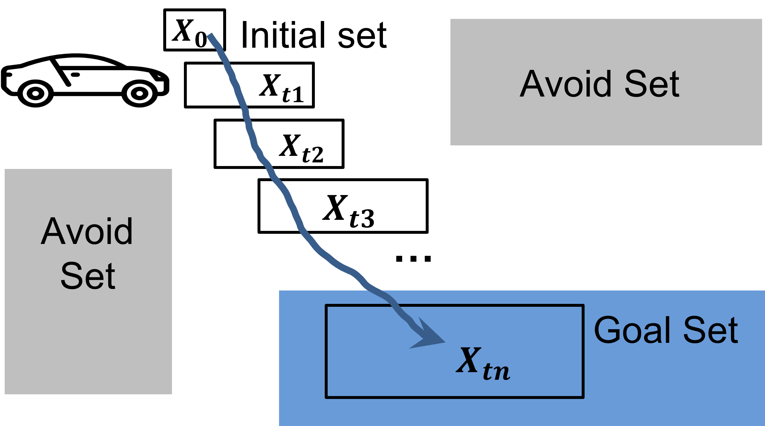
Figure 1: NNCS verification through reachable set estimation. We estimate the reachable sets $X_{t1},X_{t2},X_{t3}$ …, $X_{tn}$ at $t_{1},t_{2},t_{3}$ …, $t_{n}$. If all reachable sets do not intersect with the grey avoid set and $X_{tn}$ reaches the blue goal set, the NNCS is verified to be safe.

Compared to verification on NNCSs, verification on neural networks (NNs) is a relatively well-explored area (Ruan, Huang, and Kwiatkowska 2018; Ruan et al. 2019; Wu et al. 2020; Ruan, Yi, and Huang 2021; Zhang, Ruan, and Fieldsend 2022). Representative solutions can be categorised into constraint satisfaction based approaches (Botoeva et al. 2020; Katz et al. 2019, 2017) and approximation-based approaches (Singh et al. 2019; Gehr et al. 2018; Ryou et al. 2021; Mu et al. 2022). However, these verification approaches cannot be applied directly to NNCS. They are not workable in the scenario where the neural network is in close conjunction with other subsystems. A speciality of NNCSs is the association with control time steps. Moreover, approximation-based verification inevitably results in the accumulation of the over-approximation error with the control time evolved.

Table 1: Comparison with existing NNCS verification methods from multiple aspects

	Plant Dynamics	Discrete/Continuous	Workable Activation Functions	Core Techniques	Model-Agnostic Solution
SMC (2019)	Linear	Discrete	ReLU	SMC encoding + solver	✗
Verisig (2019)	Linear, Nonlinear	Discrete, Continuous	Sigmoid, Tanh	TM + Equivalent hybrid system transformation	✗
ReachNN (2019)	Linear, Nonlinear	Discrete, Continuous	ReLU, Sigmoid, Tanh	TM+ Bernstein polynomial	✗
Sherlock (2019)	Linear, Nonlinear	Discrete, Continuous	ReLU	TM + MILP	✗
ReachNN* (2020)	Linear, Nonlinear	Discrete, Continuous	ReLU, Sigmoid, Tanh	TM + Bernstein polynomial + parallel computation	✗
Verisig 2.0 (2021)	Linear, Nonlinear	Discrete, Continuous	Tanh, Sigmod	TM + Schrink wrapping + Preconditioning	✗
DeepNNC (Our work)	Any Lipschitz continuous systems	Continuous	Any Lipschitz continuous activations e.g., ReLU, Sigmoid, Tanh, etc.	Lipschitz optimisation	✓

Recently, some pioneering research has emerged to verify NNCSs. They first estimate the output range of the controller and then feed the range to a hybrid system verification tool. Although both groups of tools can generate a tight estimate on their isolated models, direct combination results in a loose estimate of NNCS reachable sets after a few control steps, known as the wrapping effect (Neumaier 1993).

To resolve the wrapping effect, researchers develop various methods to analyse NNCSs as a whole. Verisig (Ivanov et al. 2019) transforms the neural network into an equivalent hybrid system for verification, which can only work on Sigmoid activation function. NNV (Tran et al. 2020) uses a variety of set representations, e.g., polyhedra and zonotopes, for both the controller and the plant. Other researchers are inspired by the fact that the Taylor model approach can analyse hybrid systems with traditional controllers (Chen, Abraham, and Sankaranarayanan 2012). Thus, they applied the Taylor model for the verification of NNCSs. Representatives are ReachNN (Huang et al. 2019), ReachNN* (Fan et al. 2020), Versig 2.0 (Ivanov et al. 2021) and Sherlock (Dutta, Chen, and Sankaranarayanan 2019). However, verification approaches based on Taylor polynomials are limited to certain types of activation function. And their over-approximation errors still exist and accumulate over time.

To alleviate the above weakness, this paper proposes a novel verification method for NNCSs, called DeepNNC, taking advantage of the recent advance in Lipschitzian optimisation. As shown in Table 1, compared to the state-of-the-art NNCS verification, DeepNNC can solve linear and nonlinear NNCS with a wide range of activation functions. Essentially, we treat the reachability problem as a black-box optimisation problem and verify the NNCS as long as it is Lipschitz continuous. DeepNNC is the only model-agnostic approach, which means that access to the inner structure of NNCSs is not required. DeepNNC has the ability to work on any Lipschitz continuous complex system to achieve efficient and tight reachability analysis. The contributions of this paper are summarised below:

• This paper proposes a novel framework for the verification of NNCS, called DeepNNC. It is the first model-agnostic work that can deal with a broad class of hybrid systems with linear or nonlinear plants and neural network controllers with various types of activation functions such as ReLU, Sigmoid, and Tanh activation.

• We theoretically prove that Lipschitz continuity holds on closed-loop NNCSs. DeepNNC constructs the reachable set estimation as a series of independent global optimisation problems, which can significantly reduce the over-approximation error and the wrapping effect. We also provide a theoretical analysis on the soundness and completeness of DeepNNC.

• Our intensive experiments show that DeepNNC outperforms state-of-the-art NNCS verification approaches on various benchmarks in terms of both accuracy and efficiency. On average, DeepNNC is 768 times faster than ReachNN* (Fan et al. 2020), 37 times faster than Sherlock (Dutta, Chen, and Sankaranarayanan 2019), and 56 times faster than Verisig 2.0 (Ivanov et al. 2021) (see Table 2).

Related Work

We review the related works from the following three aspects.

SMC-based approaches transform the problem into an SMC problem (Sun, Khedr, and Shoukry 2019). First, it partitions the safe workspace, i.e., the safe set, into imaging-adapted sets. After partitioning, this method utilises an SMC encoding to specify all possible assignments of the activation functions for the given plant and NNC. However, it can only work on discrete-time linear plants with ReLU neural controller.

SDP-based and LP-based approaches SDP-based approach (Hu et al. 2020) uses a semidefinite program (SDP) for reachability analysis of NNCS. It abstracts the nonlinear components of the closed-loop system by quadratic constraints and computes the approximate reachable sets via SDP. It is limited to linear systems with NNC. LP-based approach(Everett et al. 2021) provides a linear programming-based formulation of NNCSs. It demonstrates higher efficiency and scalability than the SDP methods. However, the estimation results are less tight than SDP-based methods.

Representation-based approaches use the representation sets to serve as the input and output domains for both the controller and the hybrid system. The representative method is NNV (Tran et al. 2020), which has integrated various representation sets, such as polyhedron  (Tran et al. 2019a, c), star sets (Tran et al. 2019b) and zonotop (Singh et al. 2018). For a linear plant, NNV can provide exact reachable sets, while it can only achieve an over-approximated analysis for a nonlinear plant.

Taylor model based approaches approximate the reachable sets of NNCSs with the Taylor model (TM). Representative methods are Sherlock (Dutta, Chen, and Sankaranarayanan 2019) and Verisig 2.0 (Ivanov et al. 2021). The core concept of the Taylor model is to approximate a function with a polynomial and a worst-case error bound. TM approximation has shown impressive results in the analysis of the reachability of hybrid systems with conventional controllers (Chen, Abraham, and Sankaranarayanan 2012; Chen, Ábrahám, and Sankaranarayanan 2013) and the corresponding tool Flow*(Chen, Ábrahám, and Sankaranarayanan 2013) is widely applied. Verisig (Ivanov et al. 2019) makes use of the tool Flow*(Chen, Ábrahám, and Sankaranarayanan 2013) by transforming the NNC into a regular hybrid system without a neural network. It proves that the Sigmoid is the solution to a quadratic differential equation and applies Flow* (Chen, Ábrahám, and Sankaranarayanan 2013) on the reachability analysis of the equivalent system. Instead of directly using the TM verification tool, ReachNN (Huang et al. 2019), ReachNN* (Fan et al. 2020) and Verisig 2.0 (Ivanov et al. 2021) maintain the structure of NNCS and approximate the input and output of NNC by a polynomial and an error band, with a structure similar to the TM model. Therefore, the reachable sets of controller and plant share the same format and can be transmitted and processed in the closed loop.

Table 1 presents a detailed comparison of DeepNNC with its related work. The core technique of our method is significantly different from existing solutions, enabling DeepNNC to work on any neural network controlled system as long as it is Lipschitz continuous.

Problem Formulation

This section first describes the NNCS model and then formulates the NNCS reachability problem. We deal with a closed-loop neural network controlled system as shown in Figure 2. It consists of two parts, a plant represented by a continuous system $\dot{x}=f(x,u)$ and a neural network controller $u=\sigma(y)$. The system works in a time-triggered manner with the control step size $\delta$.

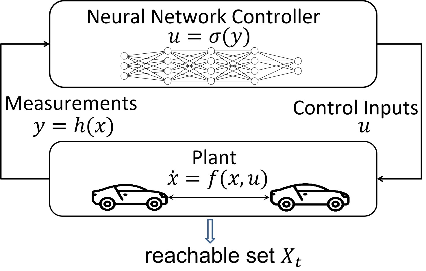
Figure 2: Architecture of a neural network controlled system. Neural network controller $\delta$ takes measurements $y$ as input and initiates the control input $u$. The plant updates its states according to its dynamic $\dot{x}=f(x,u)$ and generates new measurements of the states to be fed to the controller.

Definition 1 (Plant).

In this work, we specify the plant $P$ as a continuous system as:

$$\dot{x}=f(x,u),\quad\ x\in\mathbb{R}^{n}\ \text{and}\ u\in\mathbb{R}^{m}$$ (1)

with state $x$ containing $n$ variables, and control input $u$ consisting of $m$ variables. For the time-triggered controller, the plant dynamic inside a control time step is assigned as

$$\dot{x}(t)=f(x(t),u(i\delta))$$ (2)

with $i=0,1,2,...,$ and $t\in[i\delta,(i+1)\delta]$.

In control systems, the plant is usually modelled in the form of an ordinary differential equation (ODE). To guarantee the existence of a unique solution in ODE, the function $f$ to model the plant is required to be Lipschitz continuous in $x$ and $u$ (Meiss 2007).

Definition 2 (Neural Network Controller).

The neural network controller is a $k$ layer feedforward neural network with one or multiple types of activation functions, such as Sigmoid, Tanh, and ReLU activations, which can be defined as:

$$\sigma(y)=\sigma_{k}\circ\sigma_{k-1}\circ...\circ\sigma_{1}(y).$$ (3)

As shown in Figure 2, system transmits the measurements $y$ to the NNC, forming the control input through $u=\sigma(y)$. The measurement function $y=h(x)$ is usually Lipschitz continuous, and some systems use $y=x$ for simplicity (Ge et al. 2013).

Definition 3 (Neural Network Controlled System).

The neural network controlled system $\phi$ is a closed-loop system composed of a plant $P$ and a neural network controller $\sigma$. In a control time step, the closed-loop system is characterised as:

$$\begin{split}\phi(x(i\delta),\Delta t)&\equiv\ x(i\delta+\Delta t)\\ =x(i\delta)&+\int_{i\delta}^{i\delta+\Delta t}\ f(x(\tau),\sigma(h(x(i\delta))))\ d\tau\end{split}$$ (4)

with $i=0,1,2,3...,$ and $\Delta t\in[0,\delta]$. For a given initial state $x_{0}\in\mathcal{X}_{0}$ at $t=0$ and a specified NNCS $\phi$, the state $x$ at time $t\geq 0$ is denoted as $x(t)\equiv\phi(x_{0},t)$.

Definition 4 (Reachable Set of NNCS).

Given a range $\mathcal{X}_{0}$ for initial states and a neural network controlled system $\phi$, we define the region $S_{t}$ a reachable set at time $t\geq 0$ if all reachable states can be found in $S_{t}$.

$${\forall}x_{0}\in\mathcal{X}_{0},\ {\exists}\ \phi(x_{0},t)\in S_{t}$$ (5)

It is possible that an over-approximation of reachable states exists in the reachable set. In other words, all reachable states of time $t$ stay in $S_{t}$, while not all states in $S_{t}$ are reachable. Furthermore, we can formulate the estimation of the reachable set of NNCS as an optimisation problem:

Definition 5 (Reachability of NNCS).

Let the range $\mathcal{X}_{0}$ be initial states $x_{0}$ and $\phi$ be a NNCS. The reachability of NNCS at a predefined time point $t$ is defined as the reachable set $S_{t}(\phi,X_{0},\epsilon)=[l,u]$ of NNCS $\phi$ under an error tolerance $\epsilon\geq 0$ such that

$$\begin{split}\inf_{x_{0}\in X_{0}}\phi(x_{0},t)-\epsilon\leq l\leq\inf_{x_{0}\in X_{0}}\phi(x_{0},t)+\epsilon\\ \sup_{x_{0}\in X_{0}}\phi(x_{0},t)-\epsilon\leq u\leq\sup_{x_{0}\in X_{0}}\phi(x_{0},t)+\epsilon\end{split}$$ (6)

As discussed in multiple works (Ruan, Huang, and Kwiatkowska 2018; Katz et al. 2017), the reachability problem in neural networks is extremely challenging, it is an NP-complete problem.

Reachability Analysis via Lipschitzian Optimisation

This section presents a novel solution taking advantage of recent advances in Lipschitzian optimisation (Gergel, Grishagin, and Gergel 2016; Huang et al. 2022). But before employing Lipschitzian optimisation, we need to theoretically prove the Lipschitz continuity of the NNCS.

Lipschitz Continuity of NNCSs

Theorem 1 (Lipschitz Continuity of NNCS).

Given an initial state $X_{0}$ and a neural network controlled system $\phi(x,t)$ with controller $\sigma(x)$ and plant $f(x,u)$, if $f$ and $\sigma$ are Lipschitz continuous, then the system $\phi(x,t)$ is Lipschitz continuous in initial states $\mathcal{X}_{0}$. A real constant $K\geq 0$ exists for any time point $t>0$ and for all $x_{0},y_{0}\in\mathcal{X}_{0}$:

$$\left|\phi(x_{0},t)-\phi(y_{0},t)\right|\leq K\left|x_{0}-y_{0}\right|$$ (7)

The smallest $K$ is the best Lipschitz constant for the system, denoted $K_{best}$.

Proof.

(sketch) The essential idea is to open the control loop and further demonstrate that the system $\phi(x_{0},t)$ is Lipschitz continuous on $x_{0}$. We duplicate the NNC and plant blocks to build an equivalent open-loop control system. Based on Definition 3, we have

$$\begin{split}&\left|\phi(x_{0},t)-\phi(y_{0},t)\right|\leq\left|x_{0}-y_{0}\right|\\ +&\int_{t_{0}}^{t}\left|\ f(x(\tau),u_{x}(\tau))\ -\ f(y(\tau),u_{y}(\tau))\right|d\tau\end{split}$$ (8)

We add the term $f(x(\tau),u_{y}(\tau))\ -\ f(x(\tau),u_{y}(\tau))$ to the right side and assume that the Lipschitz constant of $f$ on $x$ and $u$ are $L_{u}$ and $L_{x}$ and the Lipschitz constant of NN as $L_{n}$, we can transform Equation (8) to the following form:

$$\begin{split}&\left\|\phi(x_{0},t)-\phi(y_{0},t)\right\|\leq\\ &(L_{u}L_{n}(t-t_{0})+1)\left\|x_{0}-y_{0}\right\|+L_{x}\int_{t_{0}}^{t}\left\|\ x(\tau)-y(\tau)\ \right\|\ d\tau.\end{split}$$ (9)

Based on Grönwall’s theory of integral inequality (Gronwall 1919), we further have the following equation:

$$\begin{split}&\left\|\phi(x_{0},t)-\phi(y_{0},t)\right\|\leq(L_{u}L_{n}(t-t_{0})+1)\left\|x_{0}-y_{0}\right\|e^{L_{x}(t-t_{0})}.\end{split}$$ (10)

Hence, we have demonstrated the Lipschitz continuity of the closed-loop system on its initial states with respect to the time interval $[0,\delta]$. We repeat this process through all the control steps and prove the Lipschitz continuity of NNCSs on initial states. See Appendix-A for a detailed proof.    ∎

Based on Theorem 1, we can easily have the following lemma about the local Lipschitz continuity of the NNCS.

Lemma 1 (Local Lipschitz Continuity of NNCS).

If NNCS $\phi(x,t)$ is Lipschitz continuous throughout $X_{0}$, then it is also locally Lipschitz continuous in its sub-intervals. There exists a real constant $k_{i}\geq 0$ for any time point $t>0$, and $\forall x_{0},y_{0}\in[a_{i},a_{i+1}]\subset X_{0}$, we have $\left\|\phi(x_{0},t)-\phi(y_{0},t)\right\|\leq k_{i}\left\|x_{0}-y_{0}\right\|$.

Based on Lemma 1, we develop a fine-grained strategy to estimate local Lipschitz constants, leading to faster convergence in Lipschitz optimisation.

Lipschitzian Optimisation

In the reachability analysis, the primary aim is to provide the lower bound $R$ of the minimal value $\phi(x),x\in X_{0}$. We achieve tighter bounds by reasonably partitioning the initial input region $X_{0}$ and evaluating the points at the edges of the partition. The pseudocode of the algorithm can be found in Appendix-B. Here, we explain the partition strategy and the construction of $R$ in the $k$-th iteration.

Figure 3: Demonstration of the optimisation process: $|\hat{\phi}_{min}^{k}-R_{min}^{k}|$ decreases with iteration $k$, optimisation converges when $|\hat{\phi}_{min}^{k}-R_{min}^{k}|<\epsilon$

• We sort the input sub intervals $D_{0},D_{1},D_{2}...D_{n}$, with $D_{i}=[a_{i},a_{i+1}]$. In the first iteration, we only have one sub interval with $D_{0}=X_{0}=[a_{0},a_{1}]$.

• We evaluate the system output $\phi_{i}=\phi_{t}(a_{i})$ at the edge points $a_{0},...a_{n}$, and define $R_{i}$ as the character value of the interval $D_{i}$ with the corresponding input $x^{R}_{i}$:

  $$R_{i}=\frac{\phi_{i}+\phi_{i+1}}{2}+l_{i}\frac{a_{i}-a_{i+1}}{2}$$ (11)

  $$x^{R}_{i}=\frac{\phi_{i}-\phi_{i+1}}{2l_{i}}+\frac{a_{i+1}+a_{i}}{2}.$$ (12)

  Both $R_{i}$ and $x^{R}_{i}$ are determined by the information of the edge point and local Lipschitz constant $l_{i}$.

• We search for the interval with a minimum character value and minimal evaluated edge points:

  $$\begin{split}&R_{min}^{k}=\min\{R_{0},...,R_{n}\},\ j=\arg\min\{R_{0},...,R_{n}\}\\ &D_{j}=[a_{j},a_{j+1}],\ \hat{\phi}_{min}^{k}=\min\{\phi_{0},\phi_{1},...\phi_{n}\}.\end{split}$$ (13)

  If $\hat{\phi}_{min}^{k}-R_{min}^{k}\leq\epsilon$, the optimisation terminates, and we return $R_{j}$ for the lower bound. Otherwise, we add a new edge point $a_{new}=x^{R}_{j}$ to divide $D_{j}$.

As illustrated in Figure 3, with blue points as edges and red points indicating the characteristic value $R$. Both $R_{min}^{k}$ and $\hat{\phi}_{min}^{k}$ are approaching the real minimum value $\phi_{min}$. The optimisation ends when $\hat{\phi}_{min}^{k}-R_{min}^{k}\leq\epsilon$, which implies $R_{min}^{k}\leq\phi_{min}\leq R_{min}^{k}+\epsilon$

To extend the above strategy into a multi-dimensional case, we use the nested optimisation scheme to solve the problem in a recursive way.

$$\min\limits_{x\in[p_{i},q_{i}]^{n}}~{}~{}\phi(x)=\min\limits_{x_{1}\in[p_{1},q_{1}]}...\min\limits_{x_{n}\in[p_{n},q_{n}]}\phi(x_{1},...,x_{n})$$ (14)

We define the $d$-th level optimisation sub-problem,

$$w_{d}(x_{1},...,x_{d})=\min_{x_{d+1}\in[p_{d+1},q_{d+1}]}w_{d+1}(x_{1},...,x_{d+1})$$ (15)

and for $d=n$, $w_{n}(x_{1},...,x_{n})=\phi(x_{1},x_{2},...,x_{n}).$ Thus, we have $\min_{{x}\in[p_{i},q_{i}]^{n}}~{}~{}\phi({x})=\min_{x_{1}\in[p_{1},q_{1}]}\phi_{1}(x_{1})$ which is actually a one-dimensional optimisation problem.

Convergence Analysis

We discuss the convergence analysis in two circumstances, i.e., one-dimensional problem and multidimensional problem. In the one-dimensional problem,we divide the sub-interval $D_{j}=[a_{j},a_{j+1}]$ into $D_{new}^{1}=[a_{j},x_{j}^{R}]$ and $D_{new}^{2}=[x_{j}^{R},a_{j+1}]$ in the $k$-th iteration. The new character value $R_{new}^{1}-R_{j}=l_{j}\frac{a_{j+1}-x_{j}^{R}}{2}-\frac{\phi_{j+1}-\phi(x_{j}^{R})}{2}>0$ , $R_{new}^{2}-R_{j}=l_{j}\frac{x_{j}^{R}-a_{j}}{2}-\frac{\phi(x_{j}^{R})-\phi_{j}}{2}>0$. Since $R_{min}^{k}=\min\{R_{0},...R_{n}\}\setminus\{R_{j}\}\}\cup\{R_{new}^{1},R_{new}^{2}\}$, we confirm that $R_{min}^{k}$ increases strictly monotonically and is bounded.

In the multidimensional problem, the problem is transformed to a one-dimensional problem with nested optimisation. We introduce Theorem 2 for the inductive step.

Theorem 2.

In optimisation, if $\forall{x}\in\mathbb{R}^{d}$, $\lim_{k\to\infty}R_{min}^{k}=\inf_{{x}\in[a,b]^{d}}\phi({x})$ and $\lim_{i\to\infty}(\hat{\phi}_{min}^{k}-R_{min}^{k})=0$ are satisfied, then $\forall x\in\mathbb{R}^{d+1}$, $\lim_{k\to\infty}R_{min}^{k}=\inf_{{x}\in[a,b]^{d+1}}\phi({x})$ and $\lim_{k\to\infty}(\hat{\phi}_{min}^{k}-R_{min}^{k})=0$ hold.

Proof.

(sketch) By the nested optimisation scheme, we have

$$\min_{\mathbf{x}\in[a_{i},b_{i}]^{d+1}}\phi(\mathbf{x})=\min_{x\in[a,b]}W(x);~{}~{}~{}W(x)=\min_{\mathbf{y}\in[a_{i},b_{i}]^{d}}\phi(x,\mathbf{y})$$ (16)

Since $\min_{\mathbf{y}\in[a_{i},b_{i}]^{d}}\phi(x,\mathbf{y})$ is bounded by an interval error $\epsilon_{\mathbf{y}}$, then we have $|W(x)-W^{*}(x)|\leq\epsilon_{\mathbf{y}},\forall x\in[a,b]$, where $W^{*}(x)$ is the accurate evaluation of the function.

For the inaccurate evaluation case, we have $W_{min}=\min_{x\in[a,b]}W(x)$, $R_{min}^{k}$ and $\widehat{W}_{min}^{k}$. The termination criteria for both cases are $|\widehat{W}^{k}_{min}-R_{min}^{k}|\leq\epsilon_{x}$ and $|\widehat{W}^{k*}_{min}-R_{min}^{k*}|\leq\epsilon_{x}$, and $w^{*}$ represents the ideal global minimum. Based on the definition of $R_{min}^{k}$, we have $w^{*}-R_{min}^{k}\leq\epsilon_{\mathbf{y}}+\epsilon_{x}$. By analogy, we get $\widehat{W}^{k}_{min}-w^{*}\leq\epsilon_{\mathbf{y}}+\epsilon_{x}$. Thus, the accurate global minimum is bounded. Theorem 2 is proved. See Appendix C for a detailed proof.    ∎

Estimation of Lipschitz Constant

To enable a fast convergence of the optimisation, we need to provide a Lipschitz constant for NNCS. As we aim for a model-agnostic reachability analysis for NNCSs, we further propose two practical variants to estimate the Lipschitz constant for a black-box NNCS.

Dynamic Estimation of Global Lipschitz Constant

In the optimisation process, the entire input range $X$ of the function $\phi_{t}(x)$ is divided into limited sub-intervals $D_{0},D_{1},D_{2}...D_{n}$, where $D_{i}=[a_{i},a_{i+1}]$. We update the global Lipschitz constant $L$ according to the interval partitions:

$$L=r\cdot max\bigg{\lvert}\frac{\phi_{t}(a_{i+1})-\phi_{t}(a_{i})}{a_{i+1}-a_{i}}\bigg{\rvert}$$ (17)

To avoid an underestimate of $L$, we choose $r>1$ and have

$$\lim_{j\to\infty}r\cdot\max_{i=1,...,j-1}\bigg{\lvert}\frac{\phi_{t}(a_{i+1})-\phi_{t}(a_{i})}{a_{i+1}-a_{i}}\bigg{\rvert}=r\cdot\sup_{a\in X}{\dfrac{d\phi_{t}}{da}}>K_{best}.$$ (18)

The dynamic update of $L$ will approximate the best Lipschitz constant of the NNCS.

Local Lipschitz Constant Estimation

An alternative to improve efficiency is the adoption of the local Lipschitz constant $l_{i}$. We adopt the local adjustment (Sergeyev 1995) for local Lipschitz estimation, which considers not only global information, but also neighbourhood intervals. For each sub-interval, we introduce $m_{i}$

$$m_{i}=|\phi_{t}(a_{i+1})-\phi_{t}(a_{i})|/|a_{i+1}-a_{i}|,M=\max\ m_{i}$$ (19)

We calculate sub-interval sizes $d_{i}$ and select the largest $D$.

$$d_{i}=\left|a_{i+1}-a_{i}\right|,D=\max\ d_{i}$$ (20)

Equation (21) estimates the local Lipschitz constant.

$$l_{i}=r\cdot\max\left\{m_{i-1},m_{i},m_{i+1},M\cdot{d_{i}}/{D}\right\}$$ (21)

It balances the local and global information. When the sub-interval is small, that is, ${M\cdot d_{i}/D}\to 0$, $l_{i}$ is decided by local information.

$$\lim_{d_{i}\to 0}l_{i}=r\cdot max\left\{m_{i-1},m_{i},m_{i+1}\right\}=r\cdot\sup_{a\in[a_{i},a_{i+1}]}{\dfrac{d\phi_{t}}{da}}>k_{i}^{best}$$

When the subinterval is large, that is, $d_{i}\to D$, local information is not reliable. $l_{i}$ is determined by global information.

$$\lim_{d_{i}\to D}l_{i}=r\cdot M=r\cdot\sup_{a\in X}{\dfrac{d\phi_{t}}{da}}>K_{best}>k_{i}^{best}$$ (22)

Local Lipschitz constants provide a more accurate polyline approximation to the original function, leading to faster convergence.

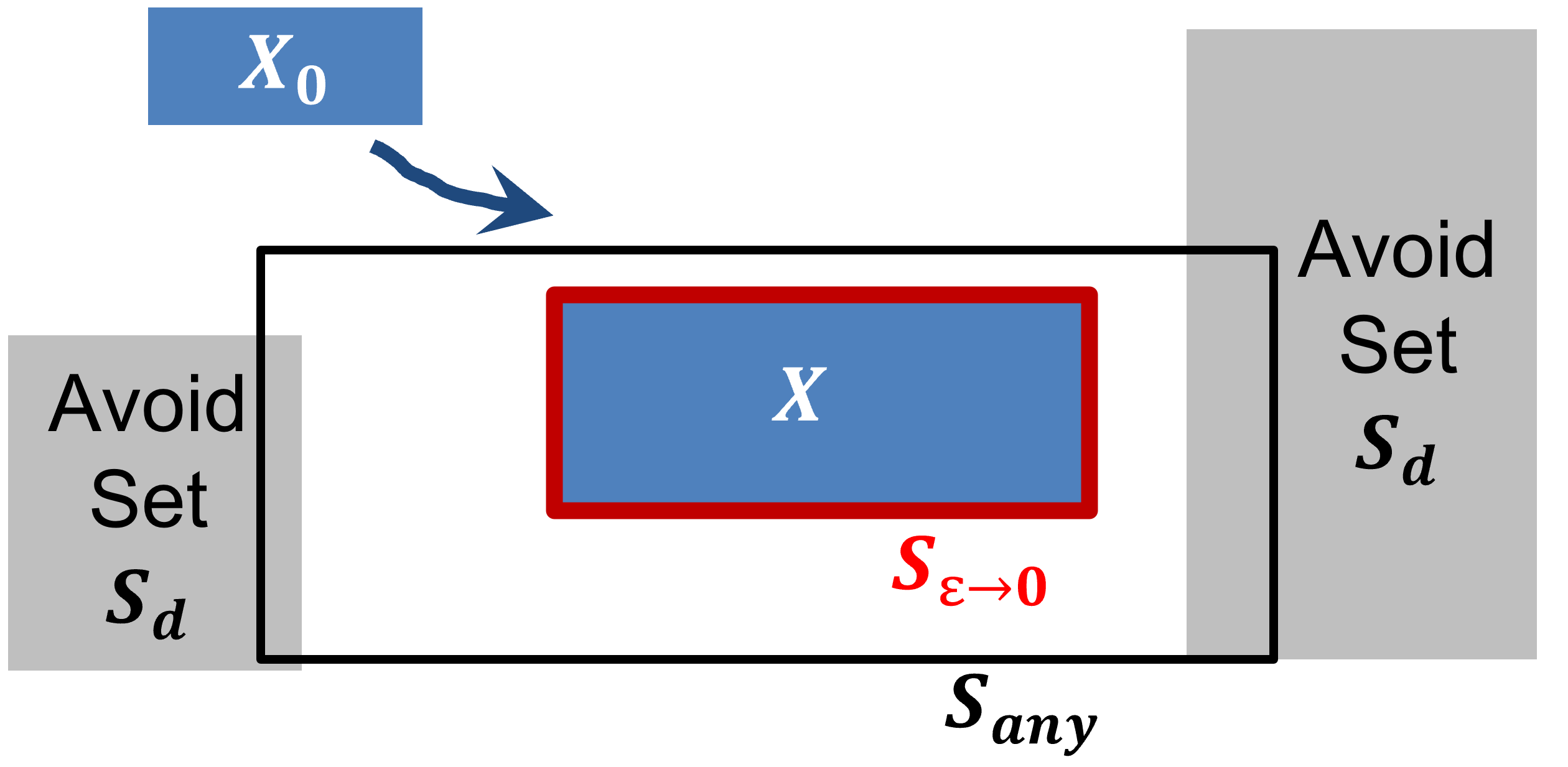
Figure 4: $X_{0}$ is the initial state set and $S_{d}$ is the avoid set. DeepNNC can return an overestimation $S_{any}$ in any iteration. Verification is sound but not complete by $S_{any}$, and Verification is both sound and complete by $S_{\epsilon\to 0}$.

Soundness and Completeness

Theorem 3 (Soundness).

Given a box-constrained initial input range $X_{0}$ and a dangerous set $S_{a}$, the verification of an NNCS via DeepNNC is sound anytime. DeepNNC can return an overestimation $S$ of the real reachable set $X$ at any iteration, even it has not reached the convergence.

Proof.

When we interrupt the optimisation at any iteration $k$, lower bound $R_{min}^{k}$ is returned for verification. We assume that the real minimal value $\phi_{min}$ is located in the sub-interval $[a_{i},a_{i+1}]$, i.e. $\phi_{min}=\phi(x_{min})$ with $x_{min}\in[a_{i},a_{i+1}]$.

$$\begin{split}&R_{i}-\phi_{min}=\frac{\phi_{i}+\phi_{i+1}}{2}-l_{i}\frac{a_{i}-a_{i+1}}{2}-\phi_{min}\\ =&\frac{\phi_{i}-\phi_{min}}{2}+l_{i}\frac{a_{i}-x_{min}}{2}+\frac{\phi_{min}-\phi_{i+1}}{2}+l_{i}\frac{x_{min}-a_{i+1}}{2}\leq 0\end{split}$$ (23)

Thus, $R_{min}^{k}-\phi_{min}\leq R_{i}-\phi_{min}\leq 0$ holds. When using $R_{min}^{k}$ to estimate the output range $S_{any}$, $R_{min}^{k}\leq\phi_{min}$ ensures $X\subset S_{any}$, where $X$ is the real reachable set. Given an avoid set $S_{d}$, if $S_{any}\cap S_{d}=\emptyset$, then $X\cap S_{d}=\emptyset$, the NNCS is safe. Thus, the approach DeepNNC is sound. ∎

Theorem 4 (Completeness).

Given a box-constrained initial input range $X_{0}$ and a dangerous set $S_{d}$, verification via DeepNNC is complete only when optimisation reaches convergence with the overestimation error $\epsilon\to 0$.

Proof.

As demonstrated in the convergence analysis, with iteration number $k\to\infty$ the optimisation can achieve convergence with error $\epsilon\to 0$. In such circumstances, the lower bound $R_{min}^{k}\to\phi_{min}$ results in an estimation $S_{\epsilon\to 0}\to X_{0}$ with ignorable estimation error. If $S_{\epsilon\to 0}\cap S_{d}\neq\emptyset$, then $X\cap S_{d}\neq\emptyset$, the NNCS is not safe.    ∎

Experiments

We first compare DeepNNC with some state-of-the-art baselines. We then analyse the influences of parameter $k_{max}$ and $\epsilon$. Finally, we provide a case study on an airplane model. An additional case study of an adaptive cruise control system is presented in Appendix D.

Comparison with State-of-the-art Methods

We test DeenNNC and baseline methods on six benchmarks. See Appendix-E for the details of the benchmarks. We compare our method with ReachNN* (Fan et al. 2020), Sherlock (Dutta et al. 2018) and Versig 2.0 (Ivanov et al. 2021) in terms of efficiency. Regarding the accuracy comparison, we compare our method with Verisig (Ivanov et al. 2019) instead of Sherlock (Dutta et al. 2018), since the results of Sherlock loose fast with the increase of control steps.

Table 2: Computation time to estimate the reachable set Tools are tested on six benchmarks and four activation functions. Results are not given if a method is not applicable or reaches the time limitation.

	Controller	DeepNNC(s)	ReachNN*(s)	Sherlock(s)	Verisig2.0(s)
1	ReLU	0.62	26	42	-
	Sigmoid	0.45	75	-	47
	Tanh	0.62	76	-	46
	ReLU+Tanh	0.60	71	-	-
2	ReLU	0.42	5	3	-
	Sigmoid	0.50	13	-	7
	Tanh	0.52	73	-	unknown
	ReLU+Tanh	0.54	8	-	-
3	ReLU	0.50	94	143	-
	Sigmoid	0.55	146	-	44
	Tanh	0.55	137	-	38
	ReLU+Tanh	0.49	unknown	-	-
4	ReLU	0.86	8	21	-
	Sigmoid	1.02	22	-	11
	Tanh	1.08	21	–	10
	ReLU+Tanh	0.98	12	-	-
5	ReLU	0.70	103	15	-
	Sigmoid	0.70	27	-	190
	Tanh	0.71	unknown	-	179
	ReLU+Tanh	0.69	unknown	-	-
6	ReLU	3.69	1130	35	-
	Sigmoid	3.62	13350	-	83
	Tanh	3.65	2416	-	70
	ReLU+Tanh	3.64	1413	-	-

The time consumption of different approaches for estimating the reachable set at a predefined time is demonstrated in Table 2 and Figure 5. Our method can be applied to all benchmarks and has relatively better efficiency, especially for low-dimensional problems.

Table 3: Area size of reachable sets. We compare the area size of the polygon reachable set at a predefined point. A smaller area size indicates a tighter estimate. The percentage is calculated by reachable set area size of (baseline - ours) / baseline, i.e., improvement of tightness of estimation.

	DeepNNC	Search	Versig2.0	Verisig	ReachNN*
B1 Sigmoid	7.7685	0.303	21	NA	145
	\	\	63.01%	NA	94.64%
B2 Sigmoid	12	5.7261	52	125	114
	\	\	76.92%	90.4%	89.47%
B5 Sigmoid	3.4762	1.7139	3.6531	8.4109	98
	\	\	4.8%	58.67%	96.45%
B5 Tanh	3.4254	1.2747	3.8021	9.1202	78
	\	\	7.28%	62.44%	95.6%
B6 Sigmoid	6.2444	3.5401	6.5366	18.324	142
	\	\	4.47%	65.92%	95.6%
B6 Tanh	6.6674	3.636	7.2116	20.343	185
	\	\	7.55%	67.23%	96.396%

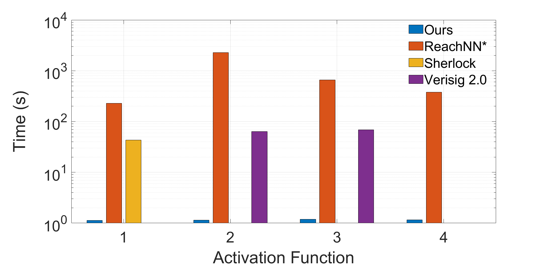
Figure 5: Average time to verify different controllers. 1. ReLU 2. Sigmoid 3. Tanh 4. ReLU+Tanh. DeepNNC is 768 times faster than ReachNN*, 37 times faster than Sherlock, 56 times faster than Verisig 2.0.

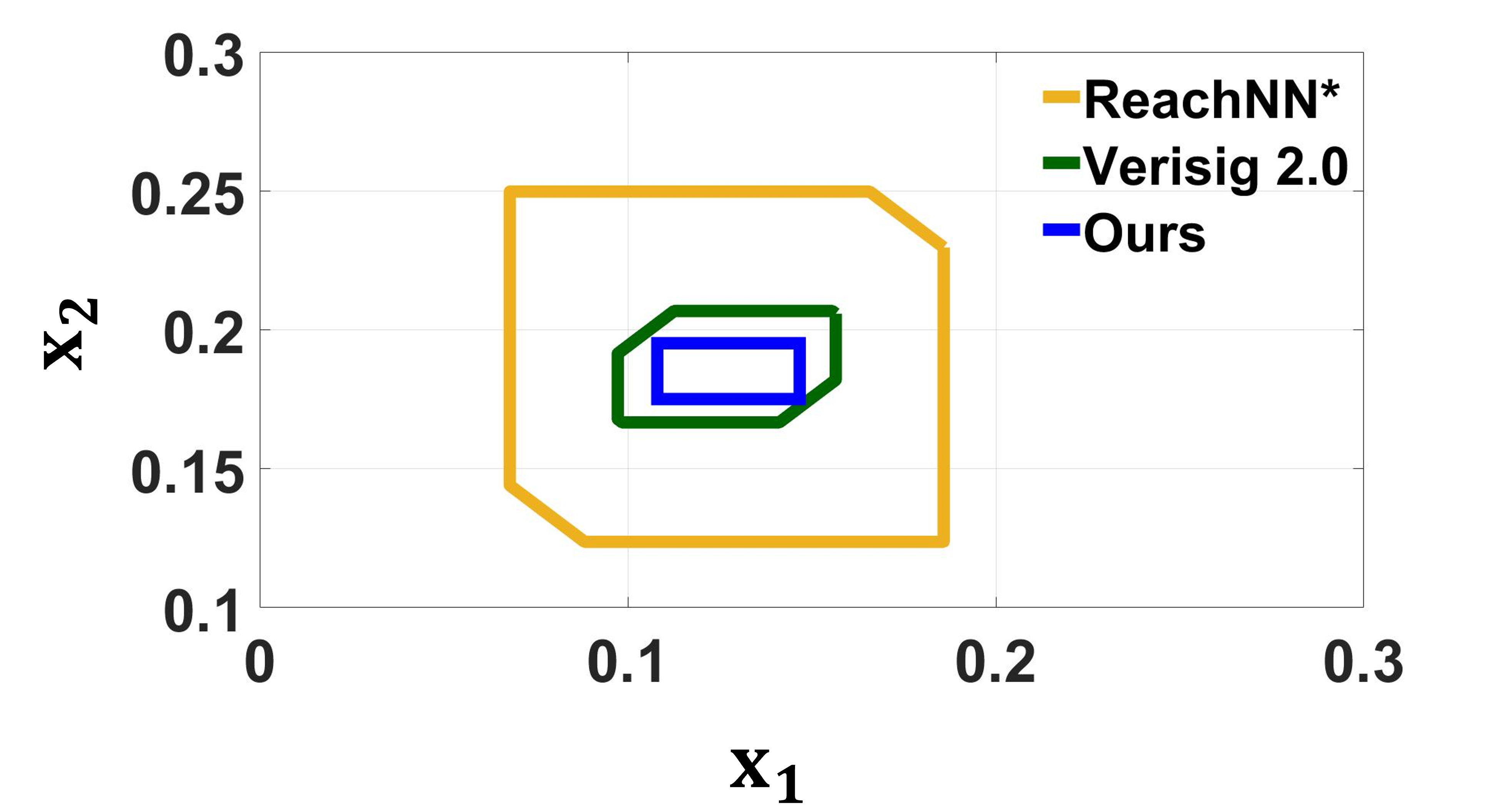
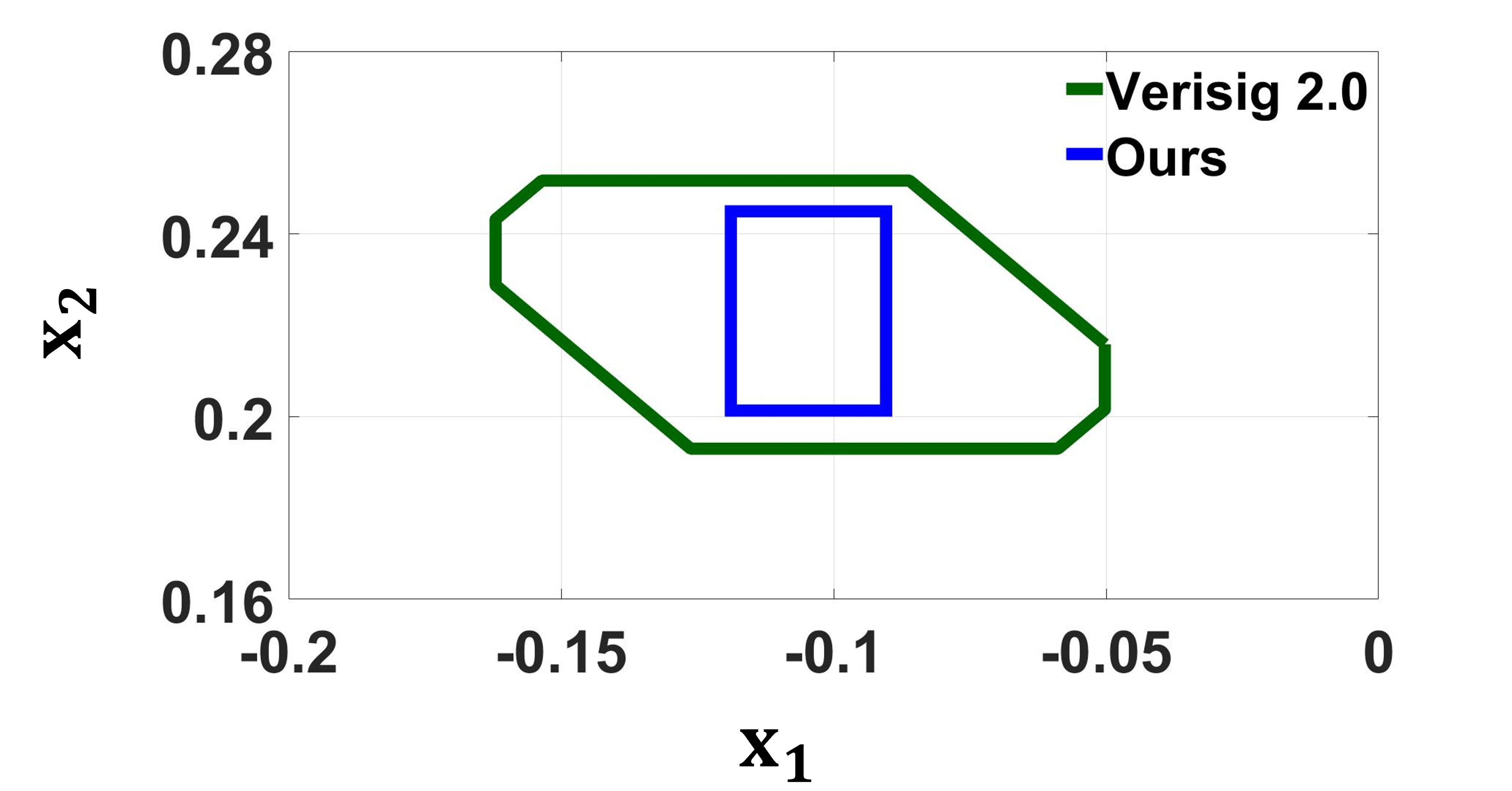
Figure 6: Reachable sets at a predefined time point estimated by different approaches. The estimated reachable set at a time point is a polygon. The size of the area of the reachable set indicates the precision of the estimation results.

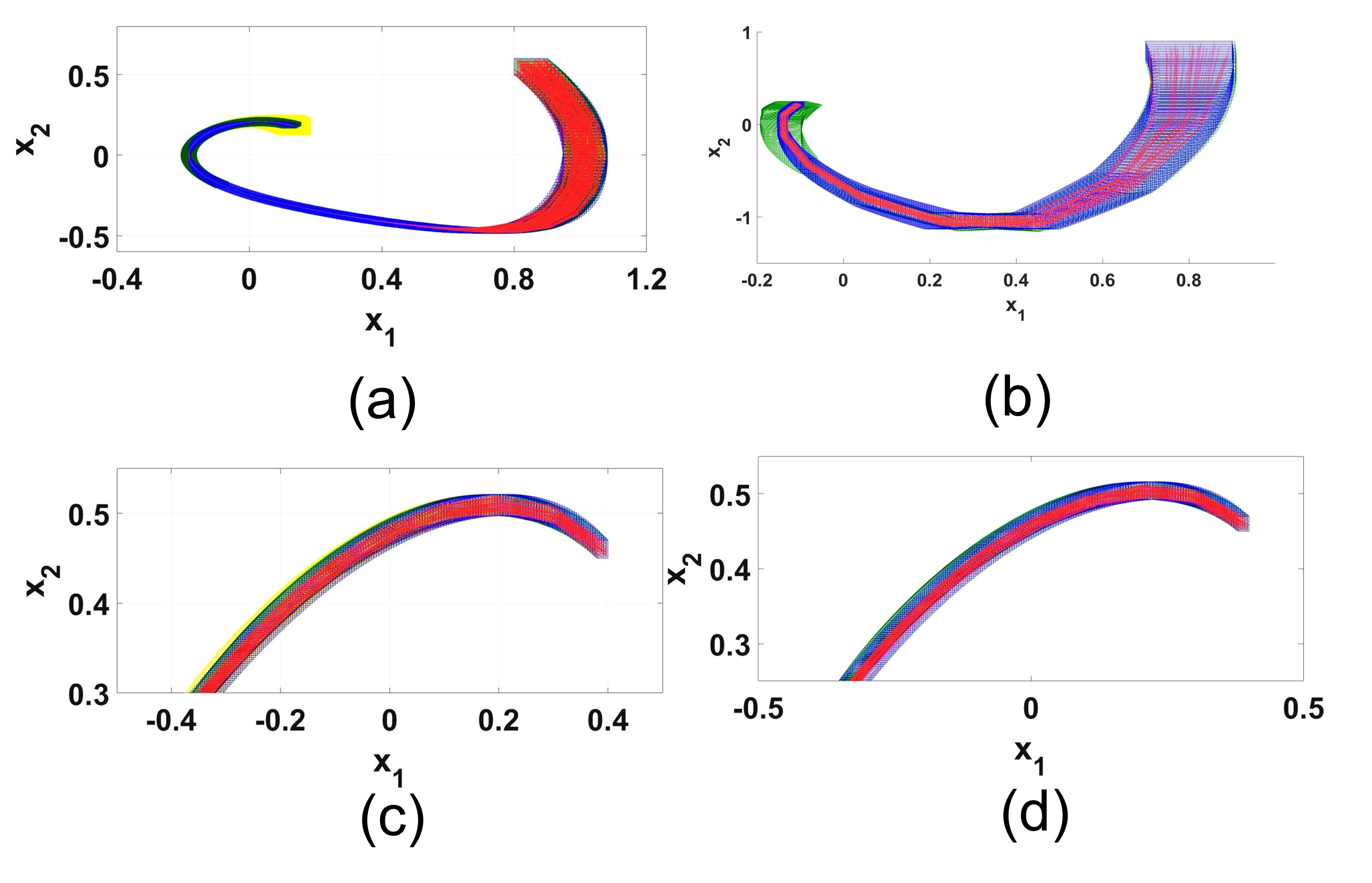
Figure 7: (a)B1 Sigmoid (b) B2 Sigmoid (c) B5 Sigmoid (d) B5 Tanh. Red trajectories are the simulated results. Blue reachable sets are generated from our approach. The yellow and green reachable sets are from the baseline methods.

We compare the accuracy of the methods by calculating the area size of the reachable set at a predefined time point. The reachable set at the same time point estimated by different approaches is demonstrated in Figure 6. The comparison of area sizes of reachable sets is presented in Table 3. Since directly obtaining an analytical ground-truth reachable set is difficult in NNCS, we use a grid-based exhaustive search with 1,000 points to approximate the ground-truth reachable set. The reachable states at the given time points are all located in the evaluated reachable set. We add a convex hull that covers all the reachable points. And we calculate and compare the area size with the reachable set. The area size of DeepNNC is slightly larger than the exhaustive search, but consistently smaller than other baselines, revealing that DeepNNC can cover all the reachable examples with a tight estimation. Figure 7 shows the reachable sets with the evolving of the control timestep and the simulated trajectories (red). Reachable sets of DeepNNC (blue) can cover the trajectories with a small overestimation error.

Impact of $\epsilon$ and $k_{max}$

Two parameters $\epsilon$ and ${}_{max}k$ are involved in our approach. $\epsilon$ indicates the allowable error, and $k_{max}$ represents the maximum number of iterations in each dimension. The iteration stops either when the difference of upper bound (red square) and lower bound (blue square) is smaller than $\epsilon$ or the iteration number in one dimension reaches $k_{max}$. In Figure 8, we fix $\epsilon=0.0005$ and change $k_{max}=3,5,10,10000$. The estimation becomes tighter with the larger iteration number. In Figure 9 we study the influence of $\epsilon$ by fixing the maximum iteration number $k_{max}=10^{4}$ and changing $\epsilon=0.5,0.05,0.005,0.0005$. The accuracy of the estimate increases with smaller $\epsilon$.

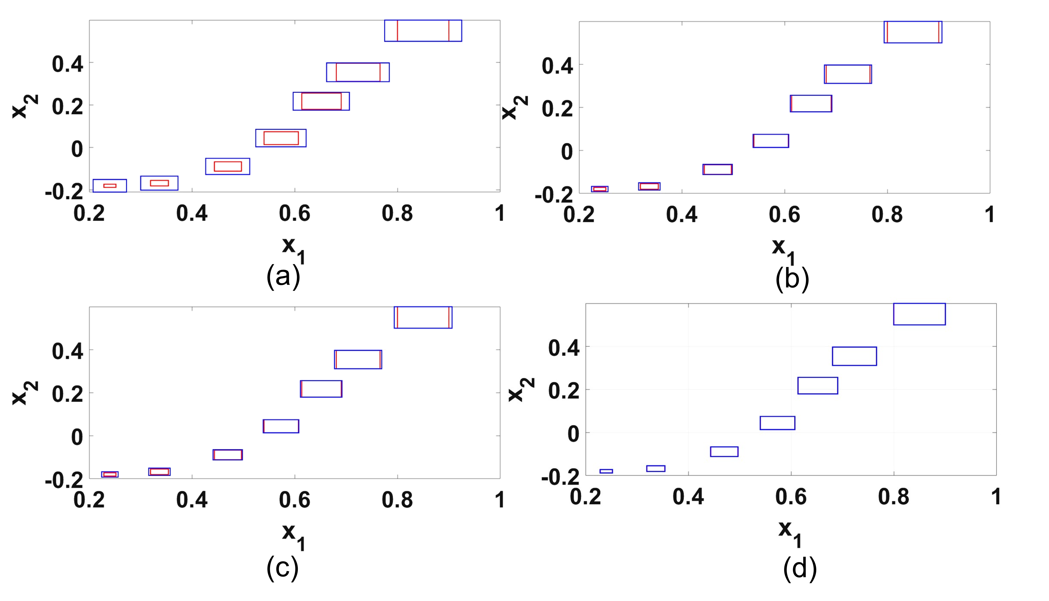
Figure 8: Reachable sets of B3 with ReLU at $t=0.01s$, 0.1s, 0.2s, 0.4s, 1s, 3s, 6s, with $\epsilon=0.0005$ and (a) $k_{max}=3$; (b) $k_{max}=5$; (c) $k_{max}=10$; (d) $k_{max}=10^{4}$

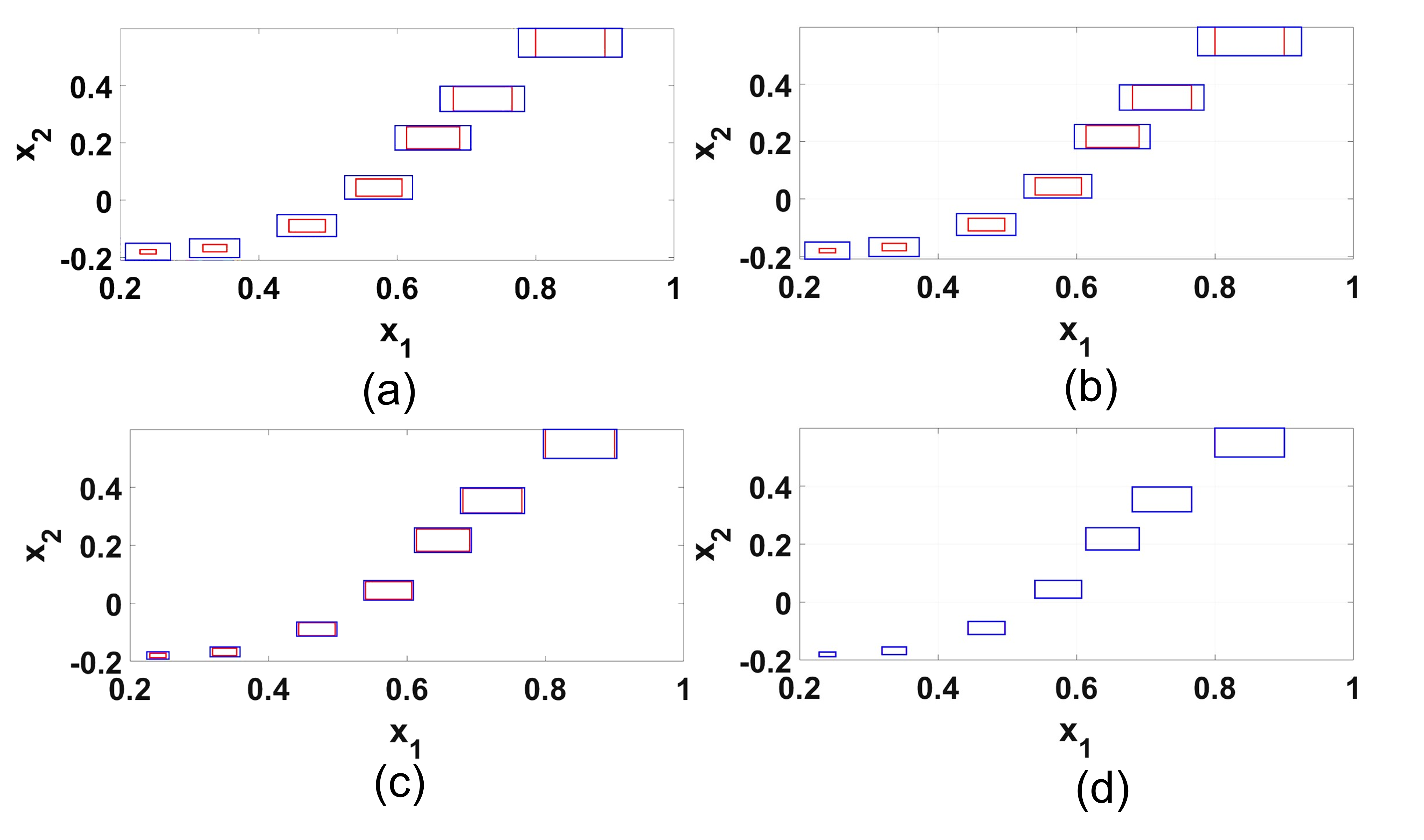
Figure 9: Reachable sets of B3 with ReLU at $t=0.01s$, 0.1s, 0.2s, 0.4s, 1s, 3s, 6s, with $k_{max}=10^{4}$ and (a) $\epsilon=0.5$; (b) $\epsilon=0.05$; (c) $\epsilon=0.005$; (d) $\epsilon=0.0005$

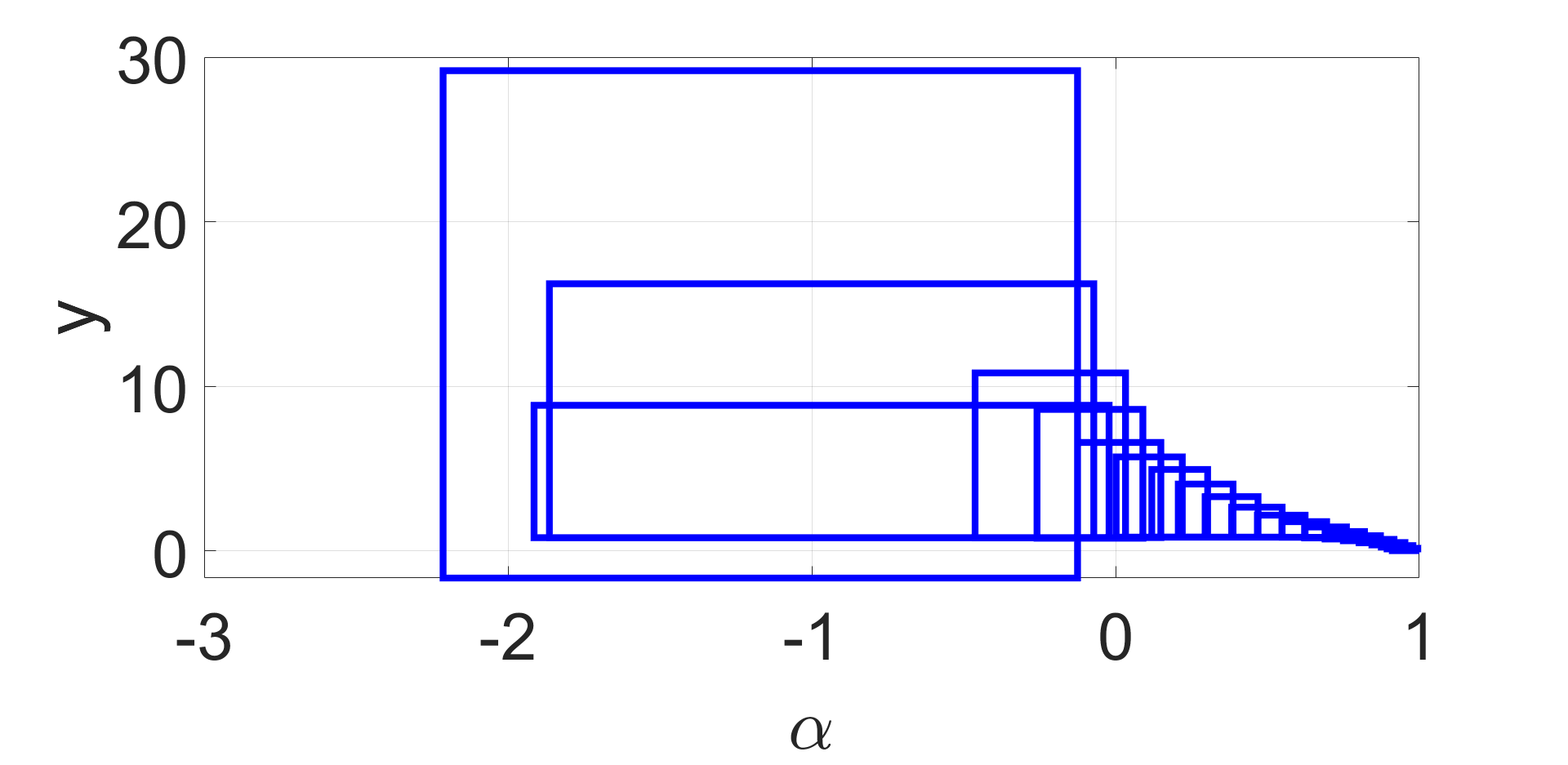
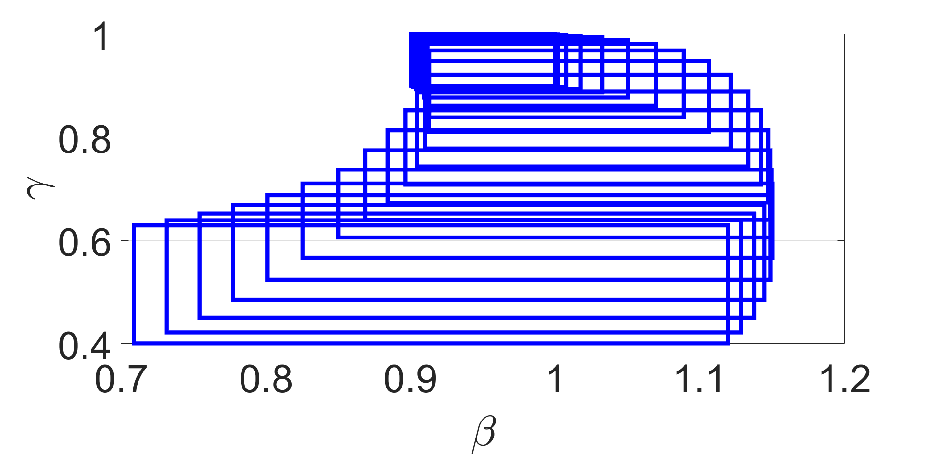
Figure 10: Reachable sets of $\alpha-y$ and $\beta$ and $\gamma$ at $t=[0s,2s]$ with an initial subset $[u,v,w,\alpha,\beta,\gamma]=[0.9,1]^{6}$

Case Study: Flying Airplane

We analyse a complex control system of a flying airplane, which is a benchmark in ARCH-COMP21 (Johnson et al. 2021). The system contains 12 states $[x,y,z,u,v,w,\alpha,\beta,\gamma,r,p,q]$ and the technical details are in Appendix-F. Initial states are $x=y=z=r=p=q=0,[u,v,w,\alpha,\beta,\gamma]=[0,1]^{6}.$ The goal set is $y\in[-0.5,0,5]$ and $[\alpha,\beta,\gamma]=[-1,1]^{3}$ for $t<2s$. The controller here takes an input of 12 dimensions and generates a six-dimensional control input $F_{x},F_{y},F_{z},M_{x},M_{y},M_{z}$. For simplicity, we choose a small subset of the initial input $[u,v,w,\alpha,\beta,\gamma]=[0.9,1]^{6}$, the estimated reachable sets of $\alpha$ and $y$ in the time range $[0s,2s]$ are presented in figure 10 (a). Both $\alpha$ and $y$ are above the safe range. Figure 10 shows the reachable set of $\alpha$ and $\gamma$, which is also above the safe region. The airplane NNCS is unsafe.

Conclusion

We develop an NNCS verification tool, DeepNNC, that is applicable to a wide range of neural network controllers, as long as the whole system is Lipschitz-continuous. We treat NNCS verification as a series of optimisation problems, and the estimated reachable set bears a tight bound even in a long control time horizon. The efficiency of DeepNNC is mainly influenced by two factors, the Lipschitz constant estimation and the dimension of the input. For the first, we have adopted dynamic local Lipschitzian optimisation to improve efficiency. Regarding the high-dimensional reachability problem, a possible solution is to transform the high-dimension problem into a one-dimensional problem using a space-filling curve (Lera and Sergeyev 2015). This idea can be explored in future work.

References

- Bojarski et al. (2016) Bojarski, M.; Del Testa, D.; Dworakowski, D.; Firner, B.; Flepp, B.; Goyal, P.; Jackel, L. D.; Monfort, M.; Muller, U.; Zhang, J.; et al. 2016. End to end learning for self-driving cars. arXiv preprint arXiv:1604.07316.
- Botoeva et al. (2020) Botoeva, E.; Kouvaros, P.; Kronqvist, J.; Lomuscio, A.; and Misener, R. 2020. Efficient verification of relu-based neural networks via dependency analysis. In Proceedings of the AAAI Conference on Artificial Intelligence, volume 34, 3291–3299.
- Chen, Abraham, and Sankaranarayanan (2012) Chen, X.; Abraham, E.; and Sankaranarayanan, S. 2012. Taylor model flowpipe construction for non-linear hybrid systems. In 2012 IEEE 33rd Real-Time Systems Symposium, 183–192. IEEE.
- Chen, Ábrahám, and Sankaranarayanan (2013) Chen, X.; Ábrahám, E.; and Sankaranarayanan, S. 2013. Flow*: An analyzer for non-linear hybrid systems. In International Conference on Computer Aided Verification, 258–263. Springer.
- Ding et al. (2019) Ding, D.; Han, Q.-L.; Wang, Z.; and Ge, X. 2019. A survey on model-based distributed control and filtering for industrial cyber-physical systems. IEEE Transactions on Industrial Informatics, 15(5): 2483–2499.
- Dutta, Chen, and Sankaranarayanan (2019) Dutta, S.; Chen, X.; and Sankaranarayanan, S. 2019. Reachability analysis for neural feedback systems using regressive polynomial rule inference. In Proceedings of the 22nd ACM International Conference on Hybrid Systems: Computation and Control, 157–168.
- Dutta et al. (2018) Dutta, S.; Jha, S.; Sankaranarayanan, S.; and Tiwari, A. 2018. Output Range Analysis for Deep Feedforward Neural Networks. In Dutle, A.; Muñoz, C.; and Narkawicz, A., eds., NASA Formal Methods, 121–138. Cham: Springer International Publishing.
- Everett et al. (2021) Everett, M.; Habibi, G.; Sun, C.; and How, J. P. 2021. Reachability analysis of neural feedback loops. IEEE Access, 9: 163938–163953.
- Fan et al. (2020) Fan, J.; Huang, C.; Chen, X.; Li, W.; and Zhu, Q. 2020. Reachnn*: A tool for reachability analysis of neural-network controlled systems. In International Symposium on Automated Technology for Verification and Analysis, 537–542. Springer.
- Ge et al. (2013) Ge, S. S.; Hang, C. C.; Lee, T. H.; and Zhang, T. 2013. Stable adaptive neural network control, volume 13. Springer Science & Business Media.
- Gehr et al. (2018) Gehr, T.; Mirman, M.; Drachsler-Cohen, D.; Tsankov, P.; Chaudhuri, S.; and Vechev, M. 2018. Ai2: Safety and robustness certification of neural networks with abstract interpretation. In 2018 IEEE Symposium on Security and Privacy (SP), 3–18. IEEE.
- Gergel, Grishagin, and Gergel (2016) Gergel, V.; Grishagin, V.; and Gergel, A. 2016. Adaptive nested optimization scheme for multidimensional global search. Journal of Global Optimization, 66(1): 35–51.
- Gronwall (1919) Gronwall, T. H. 1919. Note on the Derivatives with Respect to a Parameter of the Solutions of a System of Differential Equations. Annals of Mathematics, 20(4): 292–296.
- Hu et al. (2020) Hu, H.; Fazlyab, M.; Morari, M.; and Pappas, G. J. 2020. Reach-sdp: Reachability analysis of closed-loop systems with neural network controllers via semidefinite programming. In 2020 59th IEEE Conference on Decision and Control (CDC), 5929–5934. IEEE.
- Huang et al. (2019) Huang, C.; Fan, J.; Li, W.; Chen, X.; and Zhu, Q. 2019. Reachnn: Reachability analysis of neural-network controlled systems. ACM Transactions on Embedded Computing Systems (TECS), 18(5s): 1–22.
- Huang et al. (2020) Huang, X.; Kroening, D.; Ruan, W.; Sharp, J.; Sun, Y.; Thamo, E.; Wu, M.; and Yi, X. 2020. A survey of safety and trustworthiness of deep neural networks: Verification, testing, adversarial attack and defence, and interpretability. Computer Science Review, 37: 100270.
- Huang et al. (2022) Huang, X.; Ruan, W.; Tang, Q.; and Zhao, X. 2022. Bridging formal methods and machine learning with global optimisation. In International Conference on Formal Engineering Methods, 1–19. Springer, Cham.
- Ivanov et al. (2021) Ivanov, R.; Carpenter, T.; Weimer, J.; Alur, R.; Pappas, G.; and Lee, I. 2021. Verisig 2.0: Verification of neural network controllers using taylor model preconditioning. In International Conference on Computer Aided Verification, 249–262. Springer.
- Ivanov et al. (2019) Ivanov, R.; Weimer, J.; Alur, R.; Pappas, G. J.; and Lee, I. 2019. Verisig: verifying safety properties of hybrid systems with neural network controllers. In Proceedings of the 22nd ACM International Conference on Hybrid Systems: Computation and Control, 169–178.
- Johnson et al. (2021) Johnson, T. T.; Lopez, D. M.; Benet, L.; Forets, M.; Guadalupe, S.; Schilling, C.; Ivanov, R.; Carpenter, T. J.; Weimer, J.; and Lee, I. 2021. ARCH-COMP21 Category Report: Artificial Intelligence and Neural Network Control Systems (AINNCS) for Continuous and Hybrid Systems Plants. In Frehse, G.; and Althoff, M., eds., 8th International Workshop on Applied Verification of Continuous and Hybrid Systems (ARCH21), volume 80 of EPiC Series in Computing, 90–119. EasyChair.
- Julian et al. (2016) Julian, K. D.; Lopez, J.; Brush, J. S.; Owen, M. P.; and Kochenderfer, M. J. 2016. Policy compression for aircraft collision avoidance systems. In 2016 IEEE/AIAA 35th Digital Avionics Systems Conference (DASC), 1–10. IEEE.
- Katz et al. (2017) Katz, G.; Barrett, C.; Dill, D. L.; Julian, K.; and Kochenderfer, M. J. 2017. Reluplex: An efficient SMT solver for verifying deep neural networks. In International Conference on Computer Aided Verification, 97–117. Springer.
- Katz et al. (2019) Katz, G.; Huang, D. A.; Ibeling, D.; Julian, K.; Lazarus, C.; Lim, R.; Shah, P.; Thakoor, S.; Wu, H.; Zeljić, A.; et al. 2019. The marabou framework for verification and analysis of deep neural networks. In International Conference on Computer Aided Verification, 443–452. Springer.
- Kuutti et al. (2020) Kuutti, S.; Bowden, R.; Jin, Y.; Barber, P.; and Fallah, S. 2020. A survey of deep learning applications to autonomous vehicle control. IEEE Transactions on Intelligent Transportation Systems, 22(2): 712–733.
- Lera and Sergeyev (2015) Lera, D.; and Sergeyev, Y. D. 2015. Deterministic global optimization using space-filling curves and multiple estimates of Lipschitz and Hölder constants. Communications in Nonlinear Science and Numerical Simulation, 23(1-3): 328–342.
- Meiss (2007) Meiss, J. D. 2007. Differential dynamical systems. SIAM.
- Mu et al. (2022) Mu, R.; Ruan, W.; Marcolino, L. S.; and Ni, Q. 2022. 3DVerifier: efficient robustness verification for 3D point cloud models. Machine Learning, 1–28.
- Neumaier (1993) Neumaier, A. 1993. The wrapping effect, ellipsoid arithmetic, stability and confidence regions. In Validation numerics, 175–190. Springer.
- Ruan, Huang, and Kwiatkowska (2018) Ruan, W.; Huang, X.; and Kwiatkowska, M. 2018. Reachability analysis of deep neural networks with provable guarantees. In Proceedings of the 27th International Joint Conference on Artificial Intelligence (IJCAI’18), 2651–2659.
- Ruan et al. (2019) Ruan, W.; Wu, M.; Sun, Y.; Huang, X.; Kroening, D.; and Kwiatkowska, M. 2019. Global Robustness Evaluation of Deep Neural Networks with Provable Guarantees for the Hamming Distance. In The 28th International Joint Conference on Artificial Intelligence (IJCAI’19). IJCAI.
- Ruan, Yi, and Huang (2021) Ruan, W.; Yi, X.; and Huang, X. 2021. Adversarial Robustness of Deep Learning: Theory, Algorithms, and Applications. In Proceedings of the 30th ACM International Conference on Information & Knowledge Management (CIKM’21), 4866–4869.
- Ryou et al. (2021) Ryou, W.; Chen, J.; Balunovic, M.; Singh, G.; Dan, A.; and Vechev, M. 2021. Scalable Polyhedral Verification of Recurrent Neural Networks. In International Conference on Computer Aided Verification, 225–248. Springer.
- Schwarting, Alonso-Mora, and Rus (2018) Schwarting, W.; Alonso-Mora, J.; and Rus, D. 2018. Planning and decision-making for autonomous vehicles. Annual Review of Control, Robotics, and Autonomous Systems, 1: 187–210.
- Sergeyev (1995) Sergeyev, Y. D. 1995. An information global optimization algorithm with local tuning. SIAM Journal on Optimization, 5(4): 858–870.
- Singh et al. (2018) Singh, G.; Gehr, T.; Mirman, M.; Püschel, M.; and Vechev, M. T. 2018. Fast and Effective Robustness Certification. NeurIPS, 1(4): 6.
- Singh et al. (2019) Singh, G.; Gehr, T.; Püschel, M.; and Vechev, M. 2019. An abstract domain for certifying neural networks. Proceedings of the ACM on Programming Languages, 3(POPL): 1–30.
- Sun, Khedr, and Shoukry (2019) Sun, X.; Khedr, H.; and Shoukry, Y. 2019. Formal verification of neural network controlled autonomous systems. In Proceedings of the 22nd ACM International Conference on Hybrid Systems: Computation and Control, 147–156.
- Tran et al. (2019a) Tran, H.-D.; Cai, F.; Diego, M. L.; Musau, P.; Johnson, T. T.; and Koutsoukos, X. 2019a. Safety verification of cyber-physical systems with reinforcement learning control. ACM Transactions on Embedded Computing Systems (TECS), 18(5s): 1–22.
- Tran et al. (2019b) Tran, H.-D.; Lopez, D. M.; Musau, P.; Yang, X.; Nguyen, L. V.; Xiang, W.; and Johnson, T. T. 2019b. Star-based reachability analysis of deep neural networks. In International Symposium on Formal Methods, 670–686. Springer.
- Tran et al. (2019c) Tran, H.-D.; Musau, P.; Lopez, D. M.; Yang, X.; Nguyen, L. V.; Xiang, W.; and Johnson, T. T. 2019c. Parallelizable reachability analysis algorithms for feed-forward neural networks. In 2019 IEEE/ACM 7th International Conference on Formal Methods in Software Engineering (FormaliSE), 51–60. IEEE.
- Tran et al. (2020) Tran, H.-D.; Yang, X.; Lopez, D. M.; Musau, P.; Nguyen, L. V.; Xiang, W.; Bak, S.; and Johnson, T. T. 2020. NNV: The neural network verification tool for deep neural networks and learning-enabled cyber-physical systems. In International Conference on Computer Aided Verification, 3–17. Springer.
- Wang et al. (2022) Wang, F.; Zhang, C.; Xu, P.; and Ruan, W. 2022. Deep learning and its adversarial robustness: A brief introduction. In HANDBOOK ON COMPUTER LEARNING AND INTELLIGENCE: Volume 2: Deep Learning, Intelligent Control and Evolutionary Computation, 547–584.
- Wu and Ruan (2021) Wu, H.; and Ruan, W. 2021. Adversarial driving: Attacking end-to-end autonomous driving systems. arXiv preprint arXiv:2103.09151.
- Wu et al. (2020) Wu, M.; Wicker, M.; Ruan, W.; Huang, X.; and Kwiatkowska, M. 2020. A game-based approximate verification of deep neural networks with provable guarantees. Theoretical Computer Science, 807: 298–329.
- Yin, Ruan, and Fieldsend (2022) Yin, X.; Ruan, W.; and Fieldsend, J. 2022. DIMBA: discretely masked black-box attack in single object tracking. Machine Learning, 1–19.
- Zhang, Ruan, and Fieldsend (2022) Zhang, T.; Ruan, W.; and Fieldsend, J. E. 2022. PRoA: A Probabilistic Robustness Assessment against Functional Perturbations. In Joint European Conference on Machine Learning and Knowledge Discovery in Databases (ECML/PKDD’22).