QD3SET-1: A Database with Quantum Dissipative Dynamics Data Sets

Abstract

Simulations of the dynamics of dissipative quantum systems utilize many methods such as physics-based quantum, semiclassical, and quantum-classical as well as machine learning-based approximations, development and testing of which requires diverse data sets. Here we present a new database QD3SET-1 containing eight data sets of quantum dynamical data for two systems of broad interest, spin-boson (SB) model and the Fenna–Matthews–Olson (FMO) complex, generated with two different methods solving the dynamics, approximate local thermalizing Lindblad master equation (LTLME) and highly accurate hierarchy equations of motion (HEOM). One data set was generated with the SB model which is a two-level quantum system coupled to a harmonic environment using HEOM for 1,000 model parameters. Seven data sets were collected for the FMO complex of different sizes (7- and 8-site monomer and 24-site trimer with LTLME and 8-site monomer with HEOM) for 500–879 model parameters. Our QD3SET-1 database contains both population and coherence dynamics data and part of it has been already used for machine learning-based quantum dynamics studies.

Background & Summary

The simulation of the inherently quantum-mechanical dynamics underlying charge, energy, and coherence transfer in the condensed-phase is one of the most difficult challenges for computational physics and chemistry. The exponential scaling of the computational cost with system size makes the quantum-mechanically exact simulations of such processes in complex systems infeasible. With the exception of a few model Hamiltonians whose form makes the numerically exact quantum-dynamics simulations possible, any simulation of general condensed-phase systems must rely on approximations.[1, 2, 3, 4, 5, 6, 7, 8, 9, 10, 11, 12, 13, 14, 15, 16, 17, 18, 19, 20, 21, 22, 23, 24, 25, 26, 27, 28] Data-driven machine learning (ML) methods for quantum dynamics emerged as attractive alternative to the physics-based approximations due to their low computational cost and high accuracy. [29, 30, 31, 32, 33, 34, 35, 36, 37, 38, 39, 40, 41, 42, 43, 44, 45, 46] Development and testing of new simulation methodologies, both physics- and ML-based, would be greatly facilitated if high-quality reference quantum-dynamics data for a diverse set of quantum systems of interest were available.

Here we present a QD3SET-1 database, a collection of eight data sets of time-evolved population dynamics of the two systems: spin-boson (SB) model and the Fenna–Matthews–Olson (FMO) light-harvesting complex. The data sets are summarized in Table 1. The SB model describes a (truncated or intrinsic) two-level quantum system linearly coupled to a harmonic bath.[47, 48] The physics of both the ground state and the dynamics of the SB model is very rich. It has been a continuous object of study during the past decades. SB has become a paradigmatic model system in the development of approximate quantum-dynamics methods and, nowadays, it is becoming a popular choice for the development of ML models.[33, 40, 30]

The FMO system has become one of the most extensively studied natural light-harvesting complexes.[49, 50, 51, 52, 53, 54, 55] Under physiological conditions, the FMO complex forms a homotrimer consisting of eight bacteriochlorophyll-a (BChla) molecules per monomer. The biological function of the FMO trimer is to transfer excitation energy from the chlorosome to the reaction center (RC).[56] An interest in this light-harvesting system sparked when two-dimensional electronic spectroscopy experiments detected the presence of quantum coherence effects in the FMO complex. [57, 58, 59] These observations triggered intense debates about the role this coherence might play in the highly efficient excitation energy transfer (EET).

Early studies of the FMO complex considered only seven-site FMO models comprising of BChla 1–7. Until BChla 8 was discovered, BChla 1 and 6 were both assumed to be possible locations for accepting the excitation from the chlorosome because they are believed to be the nearest pigments to the antenna which captures the sunlight.[60, 61, 62] From there, the energy is subsequently funneled through two nearly independent routes: from site 1 to 2 (pathway 1) or from site 6 to sites 7, 5, and 4 (pathway 2). The terminal point of either route is site 3, where the exciton is then transferred to the RC.[63]

Ever since the discovery of the eighth BChla, the role of this pigment in the EET has been extensively investigated.[64, 65, 66, 67, 53, 68, 69, 63, 70] In particular, it was shown that while the population dynamics of the eight-site FMO model is markedly different from a seven-site configuration, the EET efficiencies in both models were predicted to remain comparable and very high.[63] BChla 8 has also been suggested as possible recipient of the initial excitation.

The dynamics of the FMO model has been a subject of numerous computational studies primarily focusing on understanding the role of the protein environment on the efficiency of EET (see e.g., Refs. 71, 72, 73, 74). Numerical simulations typically employ one of the several parameterized or fitted into the experimental data FMO model Hamiltonians that differ in the BChla excitation energies and the couplings between different BChla sites.[56, 75, 49, 76, 77, 78, 79] Simulations of the full FMO trimer containing 24 BChl have also been performed.[80, 81]

Reported in this Data Descriptor a QD3SET-1 database contains seven data sets of time-evolved population dynamics of FMO models with different system Hamiltonians and initial excitations for several hundreds of bath and system-bath parameters. Hierarchy of equations of motion (HEOM) approach[7, 5] was used to simulate the population dynamics of SB and FMO models, in one of the seven FMO data sets. HEOM is a numerically exact method that can describe the dynamics of a system with a non-perturbative and non-Markovian system–bath interaction. The high computational cost of HEOM, however, limits the number of FMO simulations that can be performed with this method. To generate other six FMO data sets, an approximate method—local thermalizing Lindblad master equation (LTLME)[82, 83] was used.

Some of our data was already used in previous studies developing and benchmarking ML models for quantum-dynamics simulations. [33, 32, 30, 31] Here we regenerate one of the data sets to augment with more data and provide many new data sets generated from scratch (Table 1). To facilitate their use, we organize the data sets in a coherently formatted database and provided metadata and extraction scripts. We expect our Database that accompany this Data Descriptor will serve as valuable resources in the development of new quantum-dynamics methods.

Methods

SB data set

This data set is re-generated with the same settings and the same parameters as in on our previous SB data set[33] in order to include all the elements (populations and coherences) of the system’s reduced density matrix (RDM). The populations and population differences were published and used before.[33, 30] Below we provide a brief summary for self-containing presentation of the data set.

Spin-boson model

The spin-boson model comprises a two-level quantum subsystem (TLS) coupled to a bath of harmonic oscillators. The Hamiltonian has the following standard system-bath form: $\hat{H}=\hat{H}_{s}+\hat{H}_{b}+\hat{H}_{sb}$. The Hamiltonian of the TLS in the local (or site) basis $\{|+\rangle,|-\rangle\}$ is given by ($\hslash$=1)

$$\hat{H}_{s}=\epsilon\left(|+\rangle\langle+|-|-\rangle\langle-|\right)\,+\,\Delta\left(|+\rangle\langle-|+|-\rangle\langle+|\right),$$ (1)

where $\epsilon$ is the so-called energetic bias and $\Delta$ is the tunneling splitting. The harmonic bath is an ensemble of independent harmonic oscillators

$$\hat{H}_{b}=\sum_{j=1}^{N_{b}}\left(\frac{\hat{p}_{j}^{2}}{2m_{j}}+\frac{1}{2}m_{j}\omega_{j}^{2}\hat{x}_{j}^{2}\right),$$ (2)

where $\{\hat{x}_{j}\}$ and $\{\hat{p}_{j}\}$ are the coordinates and momenta, respectively, of $N_{b}$ independent harmonic bath modes with masses $\{m_{j}\}$ and frequencies $\{\omega_{j}\}$. The TLS and bath are coupled through the additional term

$$\hat{H}_{sb}=-\sum_{j=1}^{N_{b}}c_{j}\hat{x}_{j}\left(|+\rangle\langle+|-|-\rangle\langle-|\right),$$ (3)

where $\{c_{j}\}$ are the coupling coefficients.

The effects of the bath on the dynamics of TLS are collectively determined by the spectral density function[84]

$$J(\omega)=\frac{\pi}{2}\sum_{j=1}^{N_{b}}\frac{c_{j}^{2}}{m_{j}\omega_{j}}\delta(\omega-\omega_{j}).$$ (4)

In this work we choose to employ the Debye form of the spectral density (Ohmic spectral density with the Drude–Lorentz cut-off) [85]

$$J(\omega)=2\lambda\frac{\omega\gamma}{\omega^{2}+\gamma^{2}},$$ (5)

where $\lambda$ is the bath reorganization energy, which controls the strength of system-bath coupling, and the cutoff frequency $\gamma=1/\tau_{c}$ ($\tau_{c}$ is the bath relaxation time).

All dynamical properties of the TLS can be obtained from the RDM

$$\tilde{\rho}_{\alpha\beta}(t)=\text{Tr}_{b}\langle\alpha|e^{-i\hat{H}t/\hslash}\hat{\rho}(0)e^{i\hat{H}t/\hslash}|\beta\rangle,$$ (6)

where $\alpha,\beta\in\{|+\rangle,|-\rangle\}$, $\hat{\rho}$ is the total density operator, and the trace is taken over bath degrees of freedom. For example, the commonly used in benchmark studies population difference is obtained from the RDM as follows: $p_{+}(t)-p_{-}(t)=\tilde{\rho}_{++}(t)-\tilde{\rho}_{--}(t)$.

The initial state of the total system is assumed to be a product state of the system and bath in the following form

$$\hat{\rho}(0)=\hat{\rho}_{\mathrm{s}}(0)\hat{\rho}_{\mathrm{b}}(0).$$ (7)

In Eq. (7) the bath density operator is an equilibrium canonical density operator $\hat{\rho}_{b}(0)=e^{-\beta\hat{H}_{\mathrm{b}}}/\mathrm{Tr}_{\mathrm{b}}\left[e^{-\beta\hat{H}_{\mathrm{b}}}\right]$, where $\beta=(k_{\mathrm{B}}T)^{-1}$ is the inverse temperature and $k_{\mathrm{B}}$ is the Boltzmann constant. The initial density operator of the system is chosen to be $\hat{\rho}_{\mathrm{s}}(0)=|+\rangle\langle+|$. These conditions corresponds to instantaneous photoexcitation of the subsystem.

Data generation with spin-boson model and the hierarchy equations of motion approach

The data set for the spin-boson model was generated as described previously.[33] We also summarize it below. The following system and bath parameters were chosen: $\tilde{\epsilon}=\epsilon/\Delta=\{0,1\}$, $\tilde{\lambda}=\lambda/\Delta=\{0.1,0.2,0.3,0.4,0.5,0.6,0.7,0.8,0.9,1.0\}$, $\tilde{\gamma}=\gamma/\Delta=\{1,2,3,4,5,6,7,8,9,10\}$, and $\tilde{\beta}=\beta\Delta=\{0.1,0.25,0.5,0.75,1\}$, where the tunneling matrix element $\Delta$ is set as an energy unit. For all combinations of these parameters the system’s RDM was propagated using HEOM approach implemented in QuTiP software package. [86] The total propagation time was $t_{\mathrm{max}}\Delta=20$ and the HEOM integration time-step was set to $dt\Delta=0.05$. In total, 1,000 of HEOM calculations, 500 for symmetric ($\epsilon/\Delta=0$) and 500 for asymmetric ($\epsilon/\Delta=1$) spin-boson Hamiltonian were performed. The data set contains a set of RDMs from $t\Delta=0$ to $t_{\mathrm{max}}\Delta=20$, saved every $dt\Delta=0.05$, for every combination of the parameters $(\tilde{\epsilon},\tilde{\lambda},\tilde{\gamma},\tilde{\beta})$ described above.

Fenna–Matthews–Olson complex data sets

In this section we first describe the general theory behind the FMO model Hamiltonian and later for each data set we provide specific technical details. See also Table 1 for an overview of each data set.

FMO model Hamiltonian

The FMO complex in this work is described by the system-bath Hamiltonian with the renormalization term $\hat{H}=\hat{H}_{s}+\hat{H}_{b}+\hat{H}_{sb}+\hat{H}_{ren}$. The electronic system is described by the Frenkel exciton Hamiltonian

$$\hat{H}_{s}=\sum_{n=1}^{N_{e}}E_{n}|n\rangle\langle n|+\sum_{n,m=1,n\neq m}^{N_{e}}V_{nm}|n\rangle\langle m|,$$ (8)

where $|n\rangle$ denotes that only the $n$th site is in its electronically excited state and all other sites are in their electronically ground states, $E_{n}$ are the transition energies, and $V_{nm}$ is the Coulomb coupling between $n$th and $m$th sites. The couplings are assumed to be constant (the Condon approximation). Note that the overall electronic ground state of the pigment protein complex $|0\rangle$ is assumed to be only radiatively coupled to the single-excitation manifold and as such it is not included in the dynamics calculations. In analogy with the SB model the bath is modeled by a set of independent harmonic oscillators. The thermal bath is coupled to the subsystem’s states $|n\rangle$ through the system-bath interaction term

$$\hat{H}_{sb}=\sum_{n=1}^{N_{e}}\sum_{j=1}^{N_{b}}c_{nj}\hat{x}_{j}|n\rangle\langle n|,$$ (9)

where each subsystem’s state is independently coupled to its own harmonic environment and $c_{nj}$ are the pigment-phonon coupling constants of environmental phonons local to the $n$th BChla.

The FMO model Hamiltonian contains a reorganization term which counters the shift in the minimum energy positions of harmonic oscillators introduced by the system-bath coupling. In the case that each state $|n\rangle$ is independently coupled to the environment the renormalization term takes the following form

$$\hat{H}_{ren}=\sum_{n=1}^{N_{e}}\lambda_{n}|n\rangle\langle n|,$$ (10)

where $\lambda_{n}=\sum_{j}c_{nj}^{2}/(2m_{j}\omega_{j}^{2})$ is the bath reorganization energy. The bath spectral density associated with each electronic state is assumed to be given by the Lorentz–Drude spectral density (Eq. 5).

Analogously to the SB data set the initial state of the total system is assumed to be a product state of the system and bath. The initial electronic density operator given by $\hat{\rho}_{s}(0)$ was varied as described below. The bath density operator is taken to be the equilibrium canonical density operator.

FMO-Ia, FMO-Ib, and FMO-II data sets: 7-site FMO models with the local thermalizing Lindblad master equation approach

We generated data sets for the two 7-site system ($N_{e}=7$) Hamiltonians. FMO-I data set was generated for the system Hamiltonian parameterized by Adolphs and Renger[49] and given by (in cm^-1)

$$H_{s}=\begin{pmatrix}200&-87.7&5.5&-5.9&6.7&-13.7&-9.9\\ -87.7&320&30.8&8.2&0.7&11.8&4.3\\ 5.5&30.8&0&-53.5&-2.2&-9.6&6.0\\ -5.9&8.2&-53.5&110&-70.7&-17.0&-63.6\\ 6.7&0.7&-2.2&-70.7&270&81.1&-1.3\\ -13.7&11.8&-9.6&-17.0&81.1&420&39.7\\ -9.9&4.3&6.0&-63.3&-1.3&39.7&230\end{pmatrix},$$ (11)

FMO-Ia data set comes directly from our previous studies[32, 31] and FMO-Ib data set was generated here for a broader parameter space as described below.

FMO-II data set was generated for the Hamiltonian parameterized by Cho et al.[76] which takes the following form (in cm^-1)

$$H_{s}=\begin{pmatrix}280&-106&8&-5&6&-8&-4\\ -106&420&28&6&2&13&1\\ 8&28&0&-62&-1&-9&17\\ -5&6&-62&175&-70&-19&-57\\ 6&2&-1&-70&320&40&-2\\ -8&13&-9&-19&40&360&32\\ -4&1&17&-57&-2&32&260\end{pmatrix}.$$ (12)

The diagonal offset of 12210 cm^-1 is added to both Hamiltonians. Each site is coupled to its own bath characterized by the Drude–Lorentz spectral density, Eq. 5, but the bath of each site is described by the same spectral density.

For FMO-Ia data set, the following spectral density parameters and temperatures were employed: $\lambda$ = $\{$10, 40, 70, …, 310$\}$ cm^-1, $\gamma$ = $\{$25, 50, 75, …, 300$\}$ fs rad^-1, and T = $\{$30, 50, 70, …, 310$\}$ K. For FMO-Ib and FMO-II data sets, the spectral density parameters and temperatures were: $\lambda$ = $\{$10, 40, 70, …, 520$\}$ cm^-1, $\gamma$ = $\{$25, 50, 75, …, 500$\}$ cm^-1, and T = $\{$30, 50, 70, …, 510$\}$ K.

For FMO-Ia, FMO-Ib, and FMO-II data sets, the farthest-point sampling[87] was employed to select the most distant points in the Euclidean space[32] of parameters which typically more efficiently covers relevant space compared to random sampling.[87] We choose the top 500 (most distant) combinations of ($\lambda$ , $\gamma$, $T$) based on farthest-point sampling. For each selected set of parameters the system RDM was calculated using the local thermalizing Lindblad master equation (LTLME) approach[82, 83] implemented in the quantum_HEOM package.[88, 83] Two subsets of the data set were generated, one for the initial electronic density operator $\hat{\rho}_{s}(0)=|1\rangle\langle 1|$ corresponding to the initial excitation of site-1 and the other one for the initial density operator $\hat{\rho}_{s}(0)=|6\rangle\langle 6|$ which corresponds to the initial excitation of site-6. In each case, 500 RDM trajectories were generated. The data set contains both diagonal (populations) and off-diagonal (coherences) elements of the RDM on a time grid from 0 to 1 ns (in the case of FMO-Ia) and 0 to 50 ps (in the case of FMO-Ib and FMO-II) with the 5 fs time step.

FMO-III and FMO-IV data sets: 8-site FMO models with the local thermalizing Lindblad master equation approach

Using the same LTLME-based approach, we generated a data set for two different Hamiltonians for the 8-site FMO model. The first Hamiltonian (FMO-III data set) was parameterized by Jia et al.[89] The electronic system Hamiltonian is given by (in cm^-1)

$$H_{s}=\begin{pmatrix}218&-91.0&4.1&-6.3&6.3&-8.8&-7.8&32.4\\ -91.0&81&28.7&8.2&1.0&8.8&3.4&6.3\\ 4.1&28.7&0&-46.6&-4.4&-9.3&1.3&1.3\\ -6.3&8.2&-46.6&105&-73.9&-17.7&-59.1&-1.9\\ 6.3&1.0&-4.4&-73.9&105&76.0&-3.1&4.2\\ -8.8&8.8&-9.3&-17.7&76.0&186&25.9&-11.6\\ -7.8&3.4&1.3&-59.1&-3.1&25.9&169&-11.9\\ 32.4&6.3&1.3&-1.9&4.2&-11.6&-11.9&154\end{pmatrix},$$ (13)

with the diagonal offset of 11332 cm^-1.

The FMO-IV data set was generated for the Hamiltonian parameterized by Busch et al.[64] (site energies) and Olbrich et al. [67] (excitonic couplings) and takes the following form (in cm^-1)

$$H_{s}=\begin{pmatrix}310&-80.3&3.5&-4.0&4.5&-10.2&-4.9&21.0\\ -80.3&230&23.5&6.7&0.5&7.5&1.5&3.3\\ 3.5&23.5&0&-49.8&-1.5&-6.5&1.2&0.7\\ -4.0&6.7&-49.8&180&63.4&-13.3&-42.2&-1.2\\ 4.5&0.5&-1.5&63.4&450&55.8&4.7&2.8\\ -10.2&7.5&-6.5&-13.3&55.8&320&33.0&-7.3\\ -4.9&1.5&1.2&-42.2&4.7&33.0&270&-8.7\\ 21.0&3.3&0.7&-1.2&2.8&-7.3&-8.7&505\end{pmatrix},$$ (14)

with the diagonal offset of 12195 cm^-1.

The same set of spectral density parameters and temperatures that was used in generation of the FMO-Ib and FMO-II data sets was used here. LTLME method was used to propagate system’s RDM from 0 to 50 ps with 5 fs time-step and three initial states of the electronic system were considered: sites-1, 6 and 8. The data set contains both diagonal (populations) and off-diagonal (coherences) elements of the RDM. The calculations was performed with the quantum_HEOM package[88] with some local modifications to make it compatible for the Hamiltonians with larger dimension. We will refer to this as modified-quantum_HEOM implementation.

FMO-V data set: FMO trimer with local thermalizing Lindblad master equation approach

Additionally, we also generated a data set for the FMO trimer. The overall excitonic Hamiltonian of all three subunits is given by

$$H_{s}=\begin{pmatrix}H_{A}&H_{B}&H_{B}^{T}\\ H_{B}^{T}&H_{A}&H_{B}\\ H_{B}&H_{B}^{T}&H_{A}\end{pmatrix}$$ (15)

where $H_{A}$ is the subunit Hamiltonian for which we used the same Hamiltonian as in FMO-IV data set (Eq. 14), while $H_{B}$ is the intra-subunit Hamiltonian which is taken from the work of Olbrich et al.[67] and is given by (in cm^-1)

$$H_{B}=\begin{pmatrix}1.0&0.3&-0.6&0.7&2.3&1.5&0.9&0.1\\ 1.5&-0.4&-2.5&-1.5&7.4&5.2&1.5&0.7\\ 1.4&0.1&-2.7&5.7&4.6&2.3&4.0&0.8\\ 0.3&0.5&0.7&1.9&-0.6&-0.4&1.9&-0.8\\ 0.7&0.9&1.1&-0.1&1.8&0.1&-0.7&1.3\\ 0.1&0.7&0.8&1.4&-1.4&-1.5&1.6&-1.0\\ 0.3&0.2&-0.7&4.8&-1.6&0.1&5.7&-2.3\\ 0.1&0.6&1.5&-1.1&4.0&-3.1&-5.2&3.6\end{pmatrix}.$$ (16)

We propagate dynamics with LTLME from 0 to 50 ps with 5 fs time-step for the same parameters as was adopted in calculations for the FMO-Ib—FMO-IV data sets. The calculations were performed with the modified-quantum_HEOM implementation for the initial excited sites-1, 6 and 8.

FMO-VI data set: 8-site FMO model with the hierarchy of equations of motion approach

The LTLME approach provides only approximate description of quantum dynamics of the FMO complex. Therefore, the FMO-I—FMO-V data sets are useful merely for the developing machine learning models for quantum dynamics studies. For example, they can be used to train a neural network model which can then be further improved on more accurate but smaller data sets (e.g., via transfer learning). However, LTLME dynamics cannot be used to benchmark other quantum dynamics methods. In the latter case the high-quality reference data is needed.

To generate a data set with accurate FMO dynamics we performed HEOM calculations for the 8-site FMO model with the Hamiltonian given by Eq. 14. HEOM calculations were performed using the parallel hierarchy integrator (PHI) code.[90] The initial data set was chosen on the basis of farthest-point sampling similar to how it was done in the FMO-Ib—FMO-V data sets with the only difference being that instead of 500 most distant sets of parameters that were chosen in the preparation of FMO-Ib—FMO-V data sets, 1100 most distant set of parameters were used to prepare the initial FMO-VI data set. For certain parameters, the RAM requirements exceeded the RAM of computing nodes available to us (1 TB). Therefore, such parameter sets were excluded from the data set. Excluded parameters correspond to low temperatures, high reorganization energies, and low cut-off frequency. Such strong non-Markovian regimes pose significant challenges in the computational studies of open quantum systems. Approximately 20% of the initial data set was removed because of prohibitive memory requirements. We note that even though graphics processing units (GPU) implementations of HEOM (e.g., Ref. 91) are much faster than their CPU-based counterparts, they are still limited by the small amount of memory in presently available GPUs.

For the remaining 80% of the data set HEOM calculations were performed for 2.0 ps. To speed up calculations, an adaptive integration Runge–Kutta–Fehlberg 4/5[92] (RKF45) method was used as implemented in the PHI code. Using adaptive integration reduces both the total computation time and memory requirements but can lead to artifacts if the accuracy threshold is set too large.[90] In this work the PHI default accuracy threshold of $1\cdot 10^{-6}$ was used. The initial integration time step was set to 0.1 fs. In RKF45 the integration time step is varied and, therefore, the output comprises time-evolved RDMs on an unevenly spaced time grid. To obtain the RDMs on an evenly spaced time grid of 0.1 fs, cubic-spline interpolation was used. The interpolation errors were examined on a few cases where 0.1 fs fixed time step integration was feasible. The errors in the populations were found to be less than 10^-5 which is much smaller compared to the convergence thresholds discussed below in Technical Validation. The final FMO-VI data set contains 879 entries each comprising all the populations and coherences for the RDM from 0 to 2 ps with the time-step of 0.1 fs.

Data Records

All data sets can be accessed at https://figshare.com/s/ed24594205ab87404238. The data sets are stored in standard NumPy[93] binary file format (.npy) files. The following format of file names was adopted in the SB data set 2_epsilon-X_Delta-1.0_lambda-Y_gamma-Z_beta-XX.npy, where X denotes the value of the energetic bias ($\tilde{\epsilon}$), Y is the reorganization energy $\tilde{\lambda}$, Z is the cut-off frequency $\tilde{\gamma}$, and XX is the inverse temperature $\tilde{\beta}$. The following format of file names was adopted in all FMO data sets X_initial-Y_gamma-Z_lambda-XX_temp-YY.npy, where X denotes the number of sites in the FMO model, Y is the initial state, Z is the value of bath frequency, XX is the value of reorganization energy, and YY is the temperature.

Technical Validation

Central to the HEOM approach is the assumption that the bath correlation function $C_{a}(t)$ for site $a$ can be represented by an infinite sum of exponentially decaying terms $C_{a}(t)=\sum_{k}^{\infty}c_{ak}\exp(-\nu_{ak}t)$, where $\nu_{ak}=2\pi k/\beta\hslash$ are Matsubara frequencies. Further, each exponential term leads to a set of auxiliary density matrices which take into account the non-Markovian evolution of the system’s RDM under the influence of bath. In practice, the summation must be truncated at a finite level, $K$, which is called Matsubara cut-off and the set of auxiliary density matrices needs to be truncated at a finite number $M$. In the truncated set of auxiliary matrices are indexed by $\mathbf{n}=(n_{10},\ldots,n_{1K},n_{M0},\ldots,n_{MK})$. The hierarchy truncation level is given by $L=\sum_{a=1}^{M}\sum_{k=0}^{K}n_{ak}$, where $n_{ak}$ is the index of an auxiliary density matrix. The computational cost of the HEOM method rises steeply with the hierarchy level $L$.[90]

The hierarchy truncation level $L$ depends on how non-Markovian the system is. Although, there is some guidance on how to choose the Matsubara cut-off and hierarchy truncation level based on bath and spectral density parameters,[5, 50] in practice, the values of $M$ and $K$ have to be chosen by requiring the convergence of the RDM to acceptable accuracy level. In this work HEOM calculations for the SB model were performed by setting $L=30$ for all temperatures. The Matsubara cut-off was chosen depending on the temperature as follows: for $\beta$ = 0.1 $K$ was set to 2; for $\beta=0.25,K=3$, for $\beta=0.5,K=3$, for $\beta=0.75,K=4$, and for $\beta=1.0,K=5$. These values are chosen sufficiently high to ensure the convergence of the populations with respect to $K$ and $L$. Choosing high truncation levels in the HEOM calculations of a TLS does not present a problem given the presently available computational resources.

Similar approach of taking excessively large values of $K$ and $L$, however, is infeasible in the FMO calculations because the computational cost of HEOM grows steeply with the size of the quantum system. Therefore, the following approach was adopted for the HEOM calculations of the 8-site FMO model (FMO-VI data set). Starting from $K=0$ and $L=1$, $K$ was increased until the maximum difference in the populations between calculations with $K$ and $K+1$ falls below a threshold $\Delta$, i.e.,

$$\delta=\max_{\begin{subarray}{c}n=1,\ldots,N_{el}\\ t=0,\ldots,t_{max}\end{subarray}}\bigg{|}\rho_{n,n}^{K,L}(t)-\rho_{n,n}^{K+1,L}(t)\bigg{|}<\Delta.$$ (17)

When Eq.17 is satisfied for a given $\Delta$ the convergence with respect to Matsubara cut-off is deemed to have been achieved. Then, for a fixed $K$ a series of calculations were performed with increasing values of $L$ until the maximum difference in populations between two consecutive calculations becomes less than the same threshold value $\Delta$. When this condition is satisfied the convergence with respect to hierarchy truncation level as well as the overall convergence is declared. These steps were performed in the HEOM calculations for each parameter set for an 8-site FMO model until either the overall convergence is achieved or $K$ and/or $L$ become large enough so the calculation becomes intractable exceeding RAM available on our machines (1 TB).

In this work we set the threshold $\Delta=0.01$. This threshold was chosen such that the population errors would be almost imperceptible which is illustrated in Figure 1. This data set is converged enough to be helpful in benchmarks of approximate methods describing quantum dynamics because the errors of these methods often exceed the threshold used in this work. Additionally, Figures 2 and  3 show the number of Matsubara terms and the hierarchy truncation level required for achieving the overall convergence depending on spectral density parameters and temperature.

Usage Notes

A Python package for extracting data is provided together with the data set and can be accessed at https://github.com/Arif-PhyChem/QD3SET.

Code availability

PHI code (version 1.0) used in HEOM calculations was downloaded from http://www.ks.uiuc.edu/Research/phi/. QuTip software package (version 4.6) used in HEOM calculations of the spin-boson model and was downloaded from https://qutip.org/. LTLME calculations of FMO models were performed with the basic quantum_HEOM package https://github.com/jwa7/quantum_HEOM and was modified to enable compatibility with the Hamiltonian of larger than the default dimension.

Author contributions statement

P.O.D. and A.U. conceived the idea of creating a HEOM-based spin-boson database. A.U. conceived the idea of creating LTLME-based database for FMO complex. A.A.K conceived the idea of creating an FMO dataset with the HEOM method. A.U. performed the HEOM calculations for spin-boson along with the LTLME calculations for FMO complex. A.U. wrote the provided package for easy extraction of the data. A.A.K and L.E.H.R. performed the calculations and created database files for the FMO-VI data set. All authors analysed the results. A.A.K. took the lead in writing the original draft of the manuscript. All authors reviewed and approved the manuscript.

Competing interests

The authors declare no competing interest.

Figures & Tables

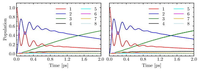
Figure 1: Example of the technical validation of the convergence of HEOM calculations for the following parameters $T=30$ K, $\lambda=70$ cm^-1, $\gamma=500$ cm^-1. The convergence within $\Delta=0.01$ threshold was achieved for $K=7$ and $L=4$. Left plot shows the populations obtained with $K=7$ and $L=4$ (solid lines) compared to populations obtained with $K=7$ and $L=5$ (dashed lines) for all 8 sites. The largest population difference is $\delta=3.14\cdot 10^{-4}$. The right plot shows the populations obtained with $K=7$ and $L=4$ (solid lines) compared to the populations obtained with $K=8$ and $L=4$. The largest population difference is $\delta=4.62\cdot 10^{-3}$. In both cases the difference is very small illustrating the validity of the chosen threshold.

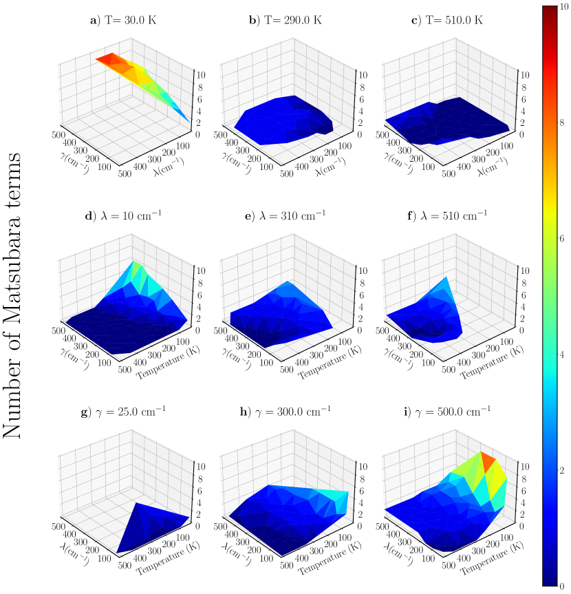
Figure 2: Number of Matsubara terms (Matsubara cut-off, $M$) required for converging populations of an 8-site FMO model with the system Hamiltonian given by Eq. 14 for three selected temperatures ($T$), reorganization energies ($\lambda$), and bath cut-off frequencies ($\gamma$).

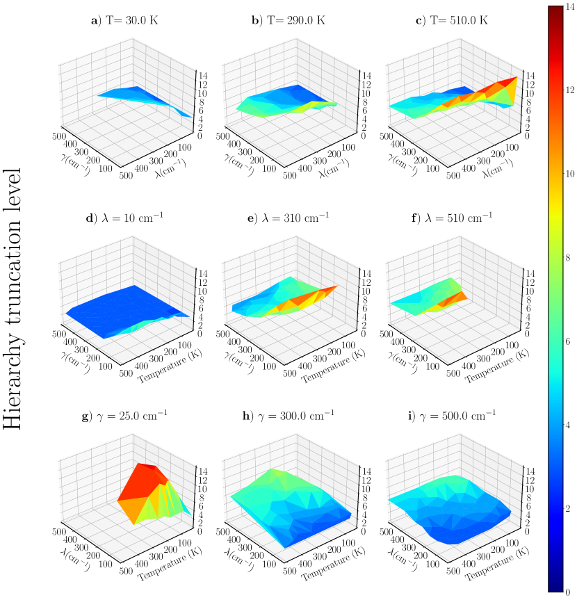
Figure 3: Hierarchy truncation level $L$ required for converging populations of an 8-site FMO model with the system Hamiltonian given by Eq. 14 for three selected temperatures ($T$), reorganization energies ($\lambda$), and bath cut-off frequencies ($\gamma$).

Data set	System	Hamiltonian(s)	Method	Data set size	Cases	Propagation time (time-step)	Package	Parameter space	References
SB	SB	SB	HEOM	1000	Symmetric and Asymmetric	20$/\Delta$ (0.05$/\Delta$)	QuTiP[86]	$\mathcal{E}^{b}$	Regenerated based on Ref. 33
FMO-Ia	7-site FMO	Adolphs and Renger[49]	LTLME		Sites 1 and 6	1 ns (5 fs)	quantum_HEOM[88, 83]	$\mathcal{F}^{c}$	Regenerated based on Ref. 32
FMO-Ib						50 ps (5 fs)	modified- quantum_HEOM a	$\mathcal{G}^{d}$	This work
FMO-II		Cho[76]
FMO-III	8-site FMO	Jia[70]
FMO-IV		Busch[64] and Olbrich[67]		1500	Sites 1, 6 and 8
FMO-V	FMO trimer
FMO-VI	8-site FMO		HEOM	879	Site 1	2 ps (0.1 fs)	PHI[90]	$\mathcal{H}^{e}$

Table 1: Summary of all data sets. See more details in the main text. Here “SB" stands for spin-boson model. ^amodified-quantum_HEOM is the quantum_HEOM package with some local modifications to make it compatible for larger Hamiltonians. ^bIn parameter space $\mathcal{E}$, we define $\tilde{\epsilon}=\epsilon/\Delta=\{0,1\}$, $\tilde{\lambda}=\lambda/\Delta=\{0.1$, $0.2$, $0.3$, $0.4$, $0.5$, $0.6$, $0.7$, $0.8$, $0.9$, $1.0\}$, $\tilde{\gamma}=\gamma/\Delta=\{1$, $2$, $3$, $4$, $5$, $6$, $7$, $8$, $9$, $10\}$, and $\tilde{\beta}=\beta\Delta=\{0.1$, $0.25$, $0.5$, $0.75$, $1\}$, where the tunneling matrix element $\Delta$ is set as an energy unit. For all combinations of these parameters the system’s RDM was propagated. ^cIn parameter space $\mathcal{F}$, we choose the top 500 (most distant) combinations of ($\lambda$ , $\gamma$, $T$) based on farthest-point sampling. Parameter range for each dimension is $\lambda$ = $\{$10, 40, 70, …, 310$\}$ cm^-1, $\gamma$ = $\{$25, 50, 75, …, 300$\}$ fs rad^-1, and T = $\{$30, 50, 70, …, 310$\}$ K. ^dIn parameter space $\mathcal{G}$, we adopt the same procedure as in parameter space $\mathcal{F}$ and choose the most distant 500 points (based on farthest-point sampling) from 3D space ($\lambda$ , $\gamma$, $T$) where $\lambda$ = $\{$10, 40, 70, …, 520$\}$ cm^-1, $\gamma$ = $\{$25, 50, 75, …, 500$\}$ cm^-1, and T = $\{$30, 50, 70, …, 510$\}$ K. ^eIn parameter space $\mathcal{H}$, parameters range remains the same as in $\mathcal{G}$. In addition, the same farthest point sampling was adopted but with the only difference being that instead of 500, 1100 most distant set of parameters were chosen. Approximately 20% of the initial data set was removed because of the prohibitive memory requirements. For the remaining 80% of the data set, HEOM calculations were performed for 2.0 ps using 0.1 fs as a time step.

References

- [1] Meyer, H., Gatti, F. & Worth, G. Multidimensional Quantum Dynamics: MCTDH Theory and Applications (Wiley, 2009).
- [2] Makri, N. Time-dependent quantum methods for large systems. \JournalTitleAnnual Review of Physical Chemistry 50, 167 – 191, 10.1146/annurev.physchem.50.1.167 (1999).
- [3] Meyer, H.-D., Manthe, U. & Cederbaum, L. The multi-configurational time-dependent Hartree approach. \JournalTitleChem. Phys. Lett. 165, 73 – 78, https://doi.org/10.1016/0009-2614(90)87014-I (1990).
- [4] Wang, H. & Thoss, M. Multilayer formulation of the multiconfiguration time-dependent hartree theory. \JournalTitleJ. Chem. Phys. 119, 1289–1299 (2003).
- [5] Tanimura, Y. Numerically “exact” approach to open quantum dynamics: The hierarchical equations of motion (HEOM). \JournalTitleJ. Chem. Phys. 153, 020901, 10.1063/5.0011599 (2020). 2006.05501.
- [6] Tanimura, Y. & Kubo, R. Two-time correlation functions of a system coupled to a heat bath with a Gaussian–Markoffian interaction. \JournalTitleProc. Jpn. Soc. 58, 1199–1206 (1989).
- [7] Tanimura, Y. Nonperturbative expansion method for a quantum system coupled to a harmonic-oscillator bath. \JournalTitlePhys. Rev. A 41, 6676–6687, 10.1103/PhysRevA.41.6676 (1990).
- [8] Greene, S. M. & Batista, V. S. Tensor-train split-operator fourier transform (tt-soft) method: Multidimensional nonadiabatic quantum dynamics. \JournalTitleJ. Chem. Theory Comput. 13, 4034–4042 (2017).
- [9] Kapral, R. PROGRESS IN THE THEORY OF MIXED QUANTUM-CLASSICAL DYNAMICS. \JournalTitleAnnual Review of Physical Chemistry 57, 129–157, 10.1146/annurev.physchem.57.032905.104702 (2006).
- [10] Kapral, R. Surface hopping from the perspective of quantum–classical Liouville dynamics. \JournalTitleChemical Physics 481, 77 – 83, 10.1016/j.chemphys.2016.05.016 (2016).
- [11] Min, S. K., Agostini, F., Tavernelli, I. & Gross, E. K. Ab initio nonadiabatic dynamics with coupled trajectories: A rigorous approach to quantum (de) coherence. \JournalTitleThe Journal of Physical Chemistry Letters 8, 3048–3055 (2017).
- [12] Min, S. K., Agostini, F. & Gross, E. K. U. Coupled-Trajectory Quantum-Classical Approach to Electronic Decoherence in Nonadiabatic Processes. \JournalTitlePhysical Review Letters 115, 073001, 10.1103/physrevlett.115.073001 (2015).
- [13] Gao, X. & Geva, E. Improving the Accuracy of Quasiclassical Mapping Hamiltonian Methods by Treating the Window Function Width as an Adjustable Parameter. \JournalTitleThe Journal of Physical Chemistry A 124, 11006–11016, 10.1021/acs.jpca.0c09750 (2020).
- [14] Crespo-Otero, R. & Barbatti, M. Recent advances and perspectives on nonadiabatic mixed quantum–classical dynamics. \JournalTitleChemical reviews 118, 7026–7068 (2018).
- [15] Subotnik, J. E. et al. Understanding the Surface Hopping View of Electronic Transitions and Decoherence. \JournalTitleAnnual Review of Physical Chemistry 67, 387 – 417, 10.1146/annurev-physchem-040215-112245 (2016).
- [16] Wang, L., Akimov, A. & Prezhdo, O. V. Recent Progress in Surface Hopping: 2011–2015. \JournalTitleThe Journal of Physical Chemistry Letters 7, 2100 – 2112, 10.1021/acs.jpclett.6b00710 (2016).
- [17] McLachlan, A. D. A variational solution of the time-dependent Schrodinger equation. \JournalTitleMolecular Physics 8, 39 – 44, 10.1080/00268976400100041 (2006).
- [18] Tully, J. C. Molecular dynamics with electronic transitions. \JournalTitleThe Journal of Chemical Physics 93, 1061–1071, 10.1063/1.459170 (1990).
- [19] Shushkov, P., Li, R. & Tully, J. C. Ring polymer molecular dynamics with surface hopping. \JournalTitleThe Journal of Chemical Physics 137, 22A549, 10.1063/1.4766449 (2012).
- [20] Huo, P., Miller, T. F. & Coker, D. F. Communication: Predictive partial linearized path integral simulation of condensed phase electron transfer dynamics. \JournalTitleThe Journal of Chemical Physics 139, 151103, 10.1063/1.4826163 (2013).
- [21] Kapral, R. & Ciccotti, G. Mixed quantum-classical dynamics. \JournalTitleThe Journal of Chemical Physics 110, 8919–8929, 10.1063/1.478811 (1999).
- [22] Miller, W. H. & Cotton, S. J. Classical molecular dynamics simulation of electronically non-adiabatic processes. \JournalTitleFaraday Discussions 195, 9 – 30, 10.1039/c6fd00181e (2016).
- [23] Sun, X. & Geva, E. Equilibrium Fermi’s Golden Rule Charge Transfer Rate Constants in the Condensed Phase: The Linearized Semiclassical Method vs Classical Marcus Theory. \JournalTitleThe Journal of Physical Chemistry A 120, 2976 – 2990, 10.1021/acs.jpca.5b08280 (2016).
- [24] Chenu, A. & Scholes, G. D. Coherence in Energy Transfer and Photosynthesis. \JournalTitleAnnu. Rev. Phys. Chem. 66, 1–28, 10.1146/annurev-physchem-040214-121713 (2015).
- [25] Han, L. et al. Stochastic equation of motion approach to fermionic dissipative dynamics. i. formalism. \JournalTitleThe Journal of Chemical Physics 152, 204105 (2020).
- [26] Ullah, A. et al. Stochastic equation of motion approach to fermionic dissipative dynamics. ii. numerical implementation. \JournalTitleThe Journal of Chemical Physics 152, 204106 (2020).
- [27] Yan, Y.-A., Zheng, X. & Shao, J. Piecewise ensemble averaging stochastic liouville equations for simulating non-markovian quantum dynamics. \JournalTitleNew Journal of Physics 24, 103012 (2022).
- [28] Chen, Z.-H., Wang, Y., Zheng, X., Xu, R.-X. & Yan, Y. Universal time-domain prony fitting decomposition for optimized hierarchical quantum master equations. \JournalTitleThe Journal of Chemical Physics 156, 221102 (2022).
- [29] Herrera Rodr’iguez, L. E. & Kananenka, A. A. Convolutional neural networks for long time dissipative quantum dynamics. \JournalTitleJ. Phys. Chem. Lett. 12, 2476–2483, 10.1021/acs.jpclett.1c00079 (2021). https://doi.org/10.1021/acs.jpclett.1c00079.
- [30] Herrera, L. E., Ullah, A., Rueda, K. J., Dral, P. O. & Kananenka, A. A comparative study of different machine learning methods for dissipative quantum dynamics. \JournalTitleMachine Learning: Science and Technology 10.1088/2632-2153/ac9a9d (2022).
- [31] Ullah, A. & Dral, P. O. One-shot trajectory learning of open quantum systems dynamics. \JournalTitleThe Journal of Physical Chemistry Letters 13, 6037–6041 (2022).
- [32] Ullah, A. & Dral, P. O. Predicting the future of excitation energy transfer in light-harvesting complex with artificial intelligence-based quantum dynamics. \JournalTitleNature Communications 13, 1–8 (2022).
- [33] Ullah, A. & Dral, P. O. Speeding up quantum dissipative dynamics of open systems with kernel methods. \JournalTitleNew Journal of Physics 10.1088/1367-2630/ac3261 (2021).
- [34] Naicker, K., Sinayskiy, I. & Petruccione, F. Machine learning for excitation energy transfer dynamics. \JournalTitlePhysical Review Research 4, 033175, 10.1103/physrevresearch.4.033175 (2022).
- [35] Akimov, A. V. Extending the Time Scales of Nonadiabatic Molecular Dynamics via Machine Learning in the Time Domain. \JournalTitleJ. Phys. Chem. Lett. 12, 12119–12128, 10.1021/acs.jpclett.1c03823 (2021).
- [36] Secor, M., Soudackov, A. V. & Hammes-Schiffer, S. Artificial Neural Networks as Propagators in Quantum Dynamics. \JournalTitleJ. Phys. Chem. Lett. 12, 10654–10662, 10.1021/acs.jpclett.1c03117 (2021).
- [37] Banchi, L., Grant, E., Rocchetto, A. & Severini, S. Modelling non-markovian quantum processes with recurrent neural networks. \JournalTitleNew J. Phys. 20, 123030, 10.1088/1367-2630/aaf749 (2018).
- [38] Bandyopadhyay, S., Huang, Z., Sun, K. & Zhao, Y. Applications of neural networks to the simulation of dynamics of open quantum systems. \JournalTitleChem. Phys. 515, 272–278 (2018).
- [39] Yang, B., He, B., Wan, J., Kubal, S. & Zhao, Y. Applications of neural networks to dynamics simulation of Landau–Zener transitions. \JournalTitleChem. Phys. 528, 110509, https://doi.org/10.1016/j.chemphys.2019.110509 (2020).
- [40] Wu, D., Hu, Z., Li, J. & Sun, X. Forecasting nonadiabatic dynamics using hybrid convolutional neural network/long short-term memory network. \JournalTitleJ. Chem. Phys. 155, 224104 (2021).
- [41] Lin, K., Peng, J., Gu, F. L. & Lan, Z. Simulation of open quantum dynamics with bootstrap-based long short-term memory recurrent neural network. \JournalTitleJ. Phys. Chem. Lett. 12, 10225–10234 (2021).
- [42] Tang, D., Jia, L., Shen, L. & Fang, W.-H. Fewest-switches surface hopping with long short-term memory networks. \JournalTitleThe Journal of Physical Chemistry Letters 13, 10377–10387, 10.1021/acs.jpclett.2c02299 (2022). PMID: 36317657, https://doi.org/10.1021/acs.jpclett.2c02299.
- [43] Lin, K., Peng, J., Xu, C., Gu, F. L. & Lan, Z. Realization of the trajectory propagation in the mm-sqc dynamics by using machine learning. \JournalTitlearXiv preprint arXiv:2207.05556 (2022).
- [44] Lin, K., Peng, J., Xu, C., Gu, F. L. & Lan, Z. Automatic evolution of machine-learning-based quantum dynamics with uncertainty analysis. \JournalTitleJournal of Chemical Theory and Computation 18, 5837–5855, 10.1021/acs.jctc.2c00702 (2022). PMID: 36184823, https://doi.org/10.1021/acs.jctc.2c00702.
- [45] Choi, M., Flam-Shepherd, D., Kyaw, T. H. & Aspuru-Guzik, A. Learning quantum dynamics with latent neural ordinary differential equations. \JournalTitlePhys. Rev. A 105, 042403, 10.1103/PhysRevA.105.042403 (2022).
- [46] Zhang, L., Ullah, A., Pinheiro Jr, M., Dral, P. O. & Barbatti, M. Excited-state dynamics with machine learning. In Quantum Chemistry in the Age of Machine Learning, 329–353 (Elsevier, 2023).
- [47] Leggett, A. J. et al. Dynamics of the dissipative two-state system. \JournalTitleRev. Mod. Phys. 59, 1–85 (1987).
- [48] Weiss, U. Quantum Dissipative Systems. Series in modern condensed matter physics (World Scientific, 2012).
- [49] Adolphs, J. & Renger, T. How proteins trigger excitation energy transfer in the fmo complex of green sulfur bacteria. \JournalTitleBiophys. J. 91, 2778–2797, https://doi.org/10.1529/biophysj.105.079483 (2006).
- [50] Ishizaki, A. & Fleming, G. R. Theoretical examination of quantum coherence in a photosynthetic system at physiological temperature. \JournalTitleProc. Natl. Acad. Sci. U.S.A. 106, 17255–17260, 10.1073/pnas.0908989106 (2009). https://www.pnas.org/content/106/41/17255.full.pdf.
- [51] Panitchayangkoon, G. et al. Long-lived quantum coherence in photosynthetic complexes at physiological temperature. \JournalTitleProc. Natl. Acad. Sci. U.S.A. 107, 12766–12770, 10.1073/pnas.1005484107 (2010). https://www.pnas.org/content/107/29/12766.full.pdf.
- [52] Harush, E. Z. & Dubi, Y. Do photosynthetic complexes use quantum coherence to increase their efficiency? Probably not. \JournalTitleSci. Adv. 7, eabc4631, 10.1126/sciadv.abc4631 (2021). https://www.science.org/doi/pdf/10.1126/sciadv.abc4631.
- [53] Ritschel, G., Roden, J., Strunz, W. T., Aspuru-Guzik, A. & Eisfeld, A. Absence of quantum oscillations and dependence on site energies in electronic excitation transfer in the Fenna–Matthews–Olson trimer. \JournalTitleJ. Phys. Chem. Lett. 2, 2912–2917, 10.1021/jz201119j (2011). https://doi.org/10.1021/jz201119j.
- [54] Shim, S., Rebentrost, P., Valleau, S. & Aspuru-Guzik, A. Atomistic study of the long-lived quantum coherences in the Fenna–Matthews–Olson complex. \JournalTitleBiophys. J. 102, 649–660, https://doi.org/10.1016/j.bpj.2011.12.021 (2012).
- [55] Fenna, R. E. & Matthews, B. W. Chlorophyll arrangement in a bacteriochlorophyll protein from Chlorobium limicola. \JournalTitleNature 258, 573–577, 10.1038/258573a0 (1975).
- [56] Milder, M. T. W., Brüggemann, B., Grondelle, R. v. & Herek, J. L. Revisiting the optical properties of the FMO protein. \JournalTitlePhotosynthesis Research 104, 257–274, 10.1007/s11120-010-9540-1 (2010).
- [57] Engel, G. S. et al. Evidence for wavelike energy transfer through quantum coherence in photosynthetic systems. \JournalTitleNature 446, 782 (2007).
- [58] Scholes, G. D. et al. Using coherence to enhance function in chemical and biophysical systems. \JournalTitleNature 543, 647–656, 10.1038/nature21425 (2017).
- [59] Engel, G. S. Quantum coherence in photosynthesis. \JournalTitleProcedia Chemistry 3, 222–231, https://doi.org/10.1016/j.proche.2011.08.029 (2011). 22nd Solvay Conference on Chemistry.
- [60] Renger, T. & May, V. Ultrafast exciton motion in photosynthetic antenna systems: the fmo-complex. \JournalTitleThe Journal of Physical Chemistry A 102, 4381–4391 (1998).
- [61] Louwe, R. J. W., Vrieze, J., Hoff, A. J. & Aartsma, T. J. Toward an integral interpretation of the optical steady-state spectra of the fmo-complex of prosthecochloris aestuarii. 2. exciton simulations. \JournalTitleThe Journal of Physical Chemistry B 101, 11280–11287, 10.1021/jp9722162 (1997). https://doi.org/10.1021/jp9722162.
- [62] List, N. H., Curutchet, C., Knecht, S., Mennucci, B. & Kongsted, J. Toward reliable prediction of the energy ladder in multichromophoric systems: A benchmark study on the fmo light-harvesting complex. \JournalTitleJournal of Chemical Theory and Computation 9, 4928–4938, 10.1021/ct400560m (2013). PMID: 26583411, https://doi.org/10.1021/ct400560m.
- [63] Moix, J., Wu, J., Huo, P., Coker, D. & Cao, J. Efficient Energy Transfer in Light-Harvesting Systems, III: The Influence of the Eighth Bacteriochlorophyll on the Dynamics and Efficiency in FMO. \JournalTitleThe Journal of Physical Chemistry Letters 2, 3045–3052, 10.1021/jz201259v (2011).
- [64] Busch, M. S. a., Mü h, F., Madjet, M. E.-A. & Renger, T. The Eighth Bacteriochlorophyll Completes the Excitation Energy Funnel in the FMO Protein. \JournalTitleThe Journal of Physical Chemistry Letters 2, 93–98, 10.1021/jz101541b (2011).
- [65] Huang, R. Y.-C., Wen, J., Blankenship, R. E. & Gross, M. L. Hydrogen–deuterium exchange mass spectrometry reveals the interaction of fenna–matthews–olson protein and chlorosome csma protein. \JournalTitleBiochemistry 51, 187–193, 10.1021/bi201620y (2012). PMID: 22142245, %****␣main.bbl␣Line␣575␣****https://doi.org/10.1021/bi201620y.
- [66] Bina, D. & Blankenship, R. E. Chemical oxidation of the FMO antenna protein from Chlorobaculum tepidum. \JournalTitlePhotosynthesis Research 116, 11–19, 10.1007/s11120-013-9878-2 (2013).
- [67] Olbrich, C. et al. From Atomistic Modeling to Excitation Transfer and Two-Dimensional Spectra of the FMO Light-Harvesting Complex. \JournalTitleThe Journal of Physical Chemistry B 115, 8609–8621, 10.1021/jp202619a (2011).
- [68] Mühlbacher, L. & Kleinekathöfer, U. Preparational effects on the excitation energy transfer in the fmo complex. \JournalTitleThe Journal of Physical Chemistry B 116, 3900–3906, 10.1021/jp301444q (2012). PMID: 22360690, https://doi.org/10.1021/jp301444q.
- [69] Tronrud, D. E., Wen, J., Gay, L. & Blankenship, R. E. The structural basis for the difference in absorbance spectra for the FMO antenna protein from various green sulfur bacteria. \JournalTitlePhotosynthesis Research 100, 79–87, 10.1007/s11120-009-9430-6 (2009).
- [70] Jia, X., Mei, Y., Zhang, J. Z. & Mo, Y. Hybrid QM/MM study of FMO complex with polarized protein-specific charge. \JournalTitleScientific Reports 5, 17096, 10.1038/srep17096 (2015).
- [71] Shabani, A., Mohseni, M., Rabitz, H. & Lloyd, S. Efficient estimation of energy transfer efficiency in light-harvesting complexes. \JournalTitlePhys. Rev. E 86, 011915, 10.1103/PhysRevE.86.011915 (2012).
- [72] Wu, J., Liu, F., Shen, Y., Cao, J. & Silbey, R. J. Efficient energy transfer in light-harvesting systems, i: optimal temperature, reorganization energy and spatial–temporal correlations. \JournalTitleNew Journal of Physics 12, 105012, 10.1088/1367-2630/12/10/105012 (2010).
- [73] Suzuki, Y., Watanabe, H., Okiyama, Y., Ebina, K. & Tanaka, S. Comparative study on model parameter evaluations for the energy transfer dynamics in Fenna–Matthews–Olson complex. \JournalTitleChemical Physics 539, 110903, 10.1016/j.chemphys.2020.110903 (2020).
- [74] Mohseni, M., Shabani, A., Lloyd, S. & Rabitz, H. Energy-scales convergence for optimal and robust quantum transport in photosynthetic complexes. \JournalTitleThe Journal of Chemical Physics 140, 035102, 10.1063/1.4856795 (2014). 1104.4812.
- [75] Vulto, S. I. E. et al. Exciton Simulations of Optical Spectra of the FMO Complex from the Green Sulfur Bacterium Chlorobium tepidum at 6 K. \JournalTitleThe Journal of Physical Chemistry B 102, 9577–9582, 10.1021/jp982095l (1998).
- [76] Cho, M., Vaswani, H. M., Brixner, T., Stenger, J. & Fleming, G. R. Exciton Analysis in 2D Electronic Spectroscopy. \JournalTitleThe Journal of Physical Chemistry B 109, 10542–10556, 10.1021/jp050788d (2005).
- [77] Hayes, D. & Engel, G. Extracting the excitonic hamiltonian of the fenna-matthews-olson complex using three-dimensional third-order electronic spectroscopy. \JournalTitleBiophysical Journal 100, 2043–2052, https://doi.org/10.1016/j.bpj.2010.12.3747 (2011).
- [78] Kell, A., Blankenship, R. E. & Jankowiak, R. Effect of spectral density shapes on the excitonic structure and dynamics of the fenna–matthews–olson trimer from chlorobaculum tepidum. \JournalTitleThe Journal of Physical Chemistry A 120, 6146–6154, 10.1021/acs.jpca.6b03107 (2016). PMID: 27438068, https://doi.org/10.1021/acs.jpca.6b03107.
- [79] Rolczynski, B. S. et al. Time-domain line-shape analysis from 2d spectroscopy to precisely determine hamiltonian parameters for a photosynthetic complex. \JournalTitleThe Journal of Physical Chemistry B 125, 2812–2820, 10.1021/acs.jpcb.0c08012 (2021). PMID: 33728918, https://doi.org/10.1021/acs.jpcb.0c08012.
- [80] Ke, Y. & Zhao, Y. Hierarchy of forward-backward stochastic schrödinger equation. \JournalTitleThe Journal of Chemical Physics 145, 024101, 10.1063/1.4955107 (2016). https://doi.org/10.1063/1.4955107.
- [81] Wilkins, D. M. & Dattani, N. S. Why quantum coherence is not important in the fenna–matthews–olsen complex. \JournalTitleJournal of Chemical Theory and Computation 11, 3411–3419, 10.1021/ct501066k (2015). PMID: 26575775, https://doi.org/10.1021/ct501066k.
- [82] Bourne Worster, S., Stross, C., Vaughan, F. M., Linden, N. & Manby, F. R. Structure and efficiency in bacterial photosynthetic light harvesting. \JournalTitleThe Journal of Physical Chemistry Letters 10, 7383–7390 (2019).
- [83] Abbott, J. W. Quantum dynamics of bath influenced excitonic energy transfer in photosynthetic pigment-protein complexes. Master Thesis, University of Bristol United Kingdom https://doi.org/10.5281/zenodo.7229807 (2020).
- [84] Caldeira, A. & Leggett, A. Path integral approach to quantum Brownian motion. \JournalTitlePhysica A: Statistical Mechanics and its Applications 121, 587–616, 10.1016/0378-4371(83)90013-4 (1983).
- [85] Wang, H., Song, X., Chandler, D. & Miller, W. H. Semiclassical study of electronically nonadiabatic dynamics in the condensed-phase: spin-boson problem with debye spectral density. \JournalTitleJ. Comp. Phys. 110, 4828 (1999).
- [86] Johansson, J., Nation, P. & Nori, F. Qutip: An open-source python framework for the dynamics of open quantum systems. \JournalTitleComput. Phys. Commun. 183, 1760–1772, https://doi.org/10.1016/j.cpc.2012.02.021 (2012).
- [87] Dral, P. O. Mlatom: A program package for quantum chemical research assisted by machine learning. \JournalTitleJournal of computational chemistry 40, 2339–2347 (2019).
- [88] Abbott, J. W. jwa7/quantum_heom. Github repository: https://github.com/jwa7/quantum_HEOM, (accessed on Nov 1, 2022) (2019).
- [89] Jia, X., Mei, Y., Zhang, J. Z. & Mo, Y. Hybrid qm/mm study of fmo complex with polarized protein-specific charge. \JournalTitleScientific reports 5, 1–10 (2015).
- [90] Strümpfer, J. & Schulten, K. Open Quantum Dynamics Calculations with the Hierarchy Equations of Motion on Parallel Computers. \JournalTitleJournal of Chemical Theory and Computation 8, 2808–2816, 10.1021/ct3003833 (2012).
- [91] Kreisbeck, C., Kramer, T., Rodr’iguez, M. & Hein, B. High-Performance Solution of Hierarchical Equations of Motion for Studying Energy Transfer in Light-Harvesting Complexes. \JournalTitleJournal of Chemical Theory and Computation 7, 2166–2174, 10.1021/ct200126d (2011). 1012.4382.
- [92] Fehlberg, E. Some old and new Runge-Kutta formulas with stepsize control and their error coefficients. \JournalTitleComputing 34, 265–270, 10.1007/bf02253322 (1985).
- [93] Oliphant, T. E. Python for scientific computing. \JournalTitleComputing in science & engineering 9, 10–20 (2007).
Acknowledgements
A.A.K. acknowledges the Ralph E. Powe Junior Faculty Enhancement Award from Oak Ridge Associated Universities. This work was also supported by General University Research (GUR) Grants and startup funds of the College of Arts and Sciences and the Department of Physics and Astronomy of the University of Delaware. P.O.D. acknowledges funding by the National Natural Science Foundation of China (No. 22003051 and funding via the Outstanding Youth Scholars (Overseas, 2021) project), the Fundamental Research Funds for the Central Universities (No. 20720210092), and via the Lab project of the State Key Laboratory of Physical Chemistry of Solid Surfaces. This research was supported in part through the use of Data Science Institute (DSI) computational resources at the University of Delaware. Calculations were also performed with high-performance computing resources provided by the Xiamen University.