Forward screening and post-screening inference in factorial designs

Abstract

Ever since the seminal work of R. A. Fisher and F. Yates, factorial designs have been an important experimental tool to simultaneously estimate the treatment effects of multiple factors. In factorial designs, the number of treatment levels may grow exponentially with the number of factors, which motivates the forward screening strategy based on the sparsity, hierarchy, and heredity principles for factorial effects. Although this strategy is intuitive and has been widely used in practice, its rigorous statistical theory has not been formally established. To fill this gap, we establish design-based theory for forward factor screening in factorial designs based on the potential outcome framework. We not only prove its consistency property but also discuss statistical inference after factor screening. In particular, with perfect screening, we quantify the advantages of forward screening based on asymptotic efficiency gain in estimating factorial effects. With imperfect screening in higher-order interactions, we propose two novel strategies and investigate their impact on subsequent inference. Our formulation differs from the existing literature on variable selection and post-selection inference because our theory is based solely on the physical randomization of the factorial design and does not rely on a correctly-specified outcome model.

Keywords: Causal inference; Design-based inference; Forward selection; Post-selection inference.

1 Introduction

1.1 Factorial experiments: opportunities and challenges

Ever since the seminal work of Fisher (1935) and Yates (1937), factorial designs have been widely used in many fields, including agricultural, industrial, and biomedical sciences (e.g., Box et al., 2005; Wu and Hamada, 2011; Gerber and Green, 2012). For example, in social science, one government funded research by Zhang (2022) studied the social construction of hate crime in the U.S. using factorial experiments based on three factors: race, sexual orientation, and religious affiliation. As another example, in ecology, Rillig et al. (2019) studied multiple global change factors in driving soil functions and microbial biodiversity with factorial designs involving up to ten factors involving drought, temperature, antibiotics, etc. Factorial experiments are popular partially because they can simultaneously accommodate multiple factors and offer opportunities to estimate not only the main causal effects of factors but also their interactions.

We focus on the $2^{K}$ factorial design in which $K$ binary factors are randomly assigned to $N$ experimental units. With a small $K$, we can simultaneously estimate the $2^{K}-1$ main effects and interactions. Nevertheless, when $K$ is large, the number of factorial effects grows exponentially with $K$. This motivates us to conduct factor screening based on sparsity, hierarchy, and heredity principles for factorial effects. More precisely, Wu and Hamada (2011) summarized these three principles as below:

1. (sparsity) The number of important factorial effects is small.

2. (hierarchy) Lower-order effects are more important than higher-order effects, and effects of the same order are equally important.

3. (heredity) Higher-order effects are significant only if their corresponding lower-order effects are significant.

The sparsity principle motivates conducting factor screening in factorial designs. The hierarchy principle motivates the forward screening strategy that starts from lower-order effects and then moves on to higher-order effects. The heredity principle motivates using structural restrictions on higher-order effects based on the selected lower-order effects. Due to its simplicity and computational efficiency, while the forward screening strategy has been widely used in data analysis (Wu and Hamada, 2011; Espinosa et al., 2016), its design-based theory under the potential outcome framework has not been formally established. Moreover, it is often challenging to understand the impact of factor screening on the subsequent statistical inference. The overarching goal of this manuscript is to fill these gaps.

1.2 Our contributions and literature review

We summarize our contribution from three perspectives:

First, our study adds to the growing literature of factorial designs with a growing number of factors under the potential outcome framework (Dasgupta et al., 2015; Branson et al., 2016; Lu, 2016b; Espinosa et al., 2016; Egami and Imai, 2019; Blackwell and Pashley, 2021; Zhao and Ding, 2021; Pashley and Bind, 2023; Wu et al., 2022). To deal with a large number of factors, Espinosa et al. (2016) and Egami and Imai (2019) informally used factor screening without studying its statistical properties, whereas Zhao and Ding (2021) discussed parsimonious model specifications that are chosen a priori and independent of data. The rigorous theory for factor screening is generally missing in this literature, let alone the theory for statistical inference after factor screening. At a high level, our contributions fill the gaps.

Second, we formalize forward factor screening and establish its consistency under the design-based framework under few outcome modeling assumptions; see Section 3. Factor screening in factorial design sounds like a familiar statistical task if we formulate it as a variable selection problem in a linear model. Thus, forward screening is reminiscent of the vast literature on forward selection. Wang (2009) and Wieczorek and Lei (2022) proved the consistency of forward selection for the main effects in a linear model, whereas Hao and Zhang (2014) and Hao et al. (2018) moved further to allow for second-order interactions. Other researchers proposed various penalized regressions to encode the sparsity, hierarchy, and heredity principles (e.g., Yuan et al., 2007; Zhao et al., 2009; Bickel et al., 2010; Bien et al., 2013; Lim and Hastie, 2015; Haris et al., 2016), without formally studying the statistical properties of the selected model. Our design-based framework departs from the literature without assuming a correctly-specified linear outcome model. This framework is classic in experimental design and causal inference with randomness coming solely from the design of experiments rather than the error terms in a linear model (Neyman, 1923/1990; Kempthorne, 1952; Freedman, 2008; Lin, 2013; Dasgupta et al., 2015). This framework invokes fewer outcome modeling assumptions but consequently imposes technical challenges for developing the theory. Bloniarz et al. (2016) discussed the design-based theory for covariate selection in treatment-control experiments, but the corresponding theory for factorial designs is largely unexplored.

Third, we discuss statistical inference after forward factor screening with (Sections 4 and 6) or without perfect screening (Section 5). On the one hand, we prove the screening consistency of the forward screening procedure, which ensures that the selected factorial effects are the true, non-zero ones. With this perfect screening property, we can then proceed as if the selected working model is the true model. This allows us to ignore the impact of forward screening on the subsequent inference, which is similar to the proposal of Zhao et al. (2021) for statistical inference after Lasso (Tibshirani, 1996). In particular, we quantify the advantages of conducting forward screening based on the asymptotic efficiency gain for estimating factorial effects. As an application under perfect screening, we discuss statistical inference for the mean outcome under the best factorial combination (Andrews et al., 2019; Guo et al., 2021; Wei et al., 2022). On the other hand, we acknowledge that perfect screening can be too much to hope for in practice as it requires strong regularity conditions on factorial effects. As a remedy, we propose two strategies to deal with imperfect screening in higher-order interactions, and we study their impacts on post-screening inference. A key motivation for our strategies is to ensure that the parameters of interest after forward factorial screening are not data-dependent, avoiding philosophical debates in the current literature of post-selection inference (Fithian et al., 2014; Kuchibhotla et al., 2022).

1.3 Notation

We will use the following notation throughout. For asymptotic analyses, $a_{N}={O}(b_{N})$ denotes that there exists a positive constant $C>0$ such that $a_{N}\leq Cb_{N}$; $a_{N}=o(b_{N})$ denotes that $a_{N}/b_{N}\to 0$ as $N$ goes to infinity; $a_{N}=\Theta(b_{N})$ denotes that there exists positive constants $c$ and $C$ such that $cb_{N}\leq a_{N}\leq Cb_{N}$.

For matrix $V$, define $\varrho_{\max}(V)$ and $\varrho_{\min}(V)$ as the largest and smallest eigenvalues, respectively, and define $\kappa(V)=\varrho_{\max}(V)/\varrho_{\min}(V)$ as its condition number. For two positive semi-definite matrices $V_{1}$ and $V_{2}$, we write $V_{1}\preccurlyeq V_{2}$ or $V_{2}\succcurlyeq V_{1}$ if $V_{2}-V_{1}$ is positive semi-definite.

We will use different levels of sets. For an integer $K$, let $[K]=\{1,\ldots,K\}$. We use ${\mathcal{K}}$ in calligraphic to denote a subset of $[K]$. Let ${\mathbb{K}}=\{{\mathcal{K}}\mid{\mathcal{K}}\subset[K]\}$ denote the power set of $[K]$. We also use blackboard bold font to denote subsets of ${\mathbb{K}}$. For example, ${\mathbb{M}}\subset{\mathbb{K}}$ denotes that ${\mathbb{M}}$ is a subset of ${\mathbb{K}}$.

We will use $A_{i}\sim B_{i}$ to denote the least-squares fit of $A_{i}$’s on $B_{i}$’s, which is purely a numerical procedure without assuming a linear model. Let $\xrightarrow{{\mathbb{P}}}$ denote convergence in probability, and $\rightsquigarrow$ denote convergence in distribution.

2 Setup of factorial designs

This section introduces the key mathematical components of factorial experiments. Section 2.1 introduces the notation of potential outcomes and the definitions of the factorial effects. Section 2.2 introduces the treatment assignment mechanism, the observed data, and the regression analysis of factorial experiment data. Section 2.3 uses a concrete example of a $2^{3}$ factorial experiment to illustrate the key concepts.

2.1 Potential outcomes and factorial effects

We first introduce the general framework of a $2^{K}$ factorial design, with $K\geq 2$ being an integer. This design has $K$ binary factors, and factor $k$ can take value $z_{k}\in\{0,1\}$ for $k=1,\ldots,K$. Let $\bm{z}=(z_{1},\dots,z_{K})$ denote the treatment combining all $K$ factors. The $K$ factors in total define $Q=2^{K}$ treatment combinations, collected in the set below:

$$\mathcal{T}=\{\bm{z}=(z_{1},\dots,z_{K})\mid z_{k}\in\{0,1\}\text{ for }k=1,\cdots,K\}\quad\text{ with }\quad|\mathcal{T}|=Q.$$

We follow the potential outcome notation of Dasgupta et al. (2015) for $2^{K}$ factorial designs. Unit $i$ has potential outcome $Y_{i}(\bm{z})$ under each treatment level $\bm{z}$. Corresponding to the $Q=2^{K}$ treatment levels, each unit $i$ has $Q$ potential outcomes, vectorized as $\bm{Y}_{i}=\{Y_{i}({\bm{z}})\}_{{\bm{z}}\in{\mathcal{T}}}$ using the lexicographic order. Over units $i=1,\ldots,N$, the potential outcomes have finite-population mean vector $\overline{Y}=(\overline{Y}({\bm{z}}))_{{\bm{z}}\in{\mathcal{T}}}$ and covariance matrix $S=(S({\bm{z}},{\bm{z}}^{\prime}))_{{\bm{z}},{\bm{z}}^{\prime}\in{\mathcal{T}}}$, with elements defined as follows:

$$\overline{Y}({\bm{z}})=\frac{1}{N}\sum_{i=1}^{N}Y_{i}({\bm{z}}),\quad S({\bm{z}},{\bm{z}}^{\prime})=\frac{1}{N-1}\sum_{i=1}^{N}(Y_{i}({\bm{z}})-\overline{Y}({\bm{z}}))(Y_{i}({\bm{z}}^{\prime})-\overline{Y}({\bm{z}}^{\prime})).$$

We then use the potential outcomes to define factorial effects. For a subset $\mathcal{K}\subset[K]$ of the $K$ factors, we introduce the following “contrast vector” notation to facilitate the presentation. To start with, we define the main causal effect for factor $k$. For a treatment level ${\bm{z}}=(z_{1},\ldots,z_{K})\in{\mathcal{T}}$, we use $g_{\{k\}}({\bm{z}})=2z_{k}-1$ to denoted the “centered” treatment indicator $z_{k}$. We then define a $Q$-dimensional contrast vector $g_{\{k\}}$ by aggregating these centered treatment variables into a vector using the lexicographic order, that is

$$g_{\{k\}}=\{g_{\{k\}}({\bm{z}})\}_{{\bm{z}}\in{\mathcal{T}}},\text{ where }g_{\{k\}}({\bm{z}})=2z_{k}-1.$$ (2.1)

Next, for the interactions of multiple factors with $|{\mathcal{K}}|\geq 2$, we define the contrast vector $g_{\mathcal{K}}\in\mathbb{R}^{Q}$ as

$$g_{\mathcal{K}}=\{g_{\mathcal{K}}({\bm{z}})\}_{{\bm{z}}\in{\mathcal{T}}},\text{ where }g_{{\mathcal{K}}}({\bm{z}})=\prod_{k\in{\mathcal{K}}}g_{\{k\}}({\bm{z}}).$$ (2.2)

As a special case, when no factor is considered, we define $g_{\varnothing}={\bm{1}}_{Q}$. Stack the contrast vectors into a $Q\times Q$ matrix

$$G=(g_{\varnothing},g_{\{1\}},\ldots,g_{\{K\}},g_{\{1,2\}},\ldots,g_{\{K-1,K\}},\ldots,g_{[K]}),$$

which has orthogonal columns with $G^{\top}G=Q\cdot I_{Q}$. We refer to $G$ as the contrast matrix.

Equipped with the contrast vector notation, we are ready to introduce the main effects and interactions. More concretely, define the main causal effect of a single factor and the $k$-way interaction causal effect of multiple factors ($k\geq 2$) as the inner product of the contrast vector $g_{\mathcal{K}}$, and the averaged potential outcome $\overline{Y}$, that is

$$\tau_{\mathcal{K}}=Q^{-1}\cdot g_{\mathcal{K}}^{\top}\overline{Y}\quad\text{ for }\quad{\mathcal{K}}\subset[K].$$ (2.3)

For convenience in description, we use $\tau_{\varnothing}=Q^{-1}g_{\varnothing}^{\top}\overline{Y}$ to denote the average of potential outcomes. We call the effect $\tau_{\mathcal{K}}$ a parent of $\tau_{{\mathcal{K}}^{\prime}}$ if ${\mathcal{K}}\subset{\mathcal{K}}^{\prime}$ and $|{\mathcal{K}}|=|{\mathcal{K}}^{\prime}|-1$. More compactly, we summarize the entire collection of causal parameters in factorial experiments as

$$\tau=(\tau_{\mathcal{K}})_{\mathcal{K}\subset[K]}=Q^{-1}\cdot{G}^{\top}\overline{Y}.$$ (2.4)

2.2 Treatment assignment, observed data, and regression analysis

Under the design-based framework, the treatment assignment mechanism characterizes the completely randomized factorial design. In other words, the experimenter randomly assigns $N(\bm{z})$ units to treatment level $\bm{z}\in\mathcal{T}$, with $\sum_{\bm{z}\in\mathcal{T}}N(\bm{z})=N$. Assume $N({\bm{z}})\geq 2$ to allow for variance estimation within each treatment level. Let $Z_{i}\in\mathcal{T}$ denote the treatment level for unit $i$. The treatment vector $(Z_{1},\ldots,Z_{N})$ is a random permutation of a vector with prespecified number $N(\bm{z})$ of the corresponding treatment level ${\bm{z}}$, for $\bm{z}\in\mathcal{T}$.

For each unit $i$, the treatment level $Z_{i}$ only reveals one potential outcome. We use $Y_{i}=Y_{i}(Z_{i})=\sum_{{\bm{z}}\in{\mathcal{T}}}Y_{i}({\bm{z}})\bm{1}\left\{Z_{i}={\bm{z}}\right\}$ to denote the observed outcome. We also use $N_{i}=N(Z_{i})$ to denote the number of units for the treatment group in which unit $i$ is assigned to. The central task of causal inference in factorial designs is to use the observed data $(Z_{i},Y_{i})_{i=1}^{N}$ to estimate factorial effects. Define

$${\widehat{Y}}({\bm{z}})=N({\bm{z}})^{-1}\sum_{i=1}^{N}\bm{1}\left\{Z_{i}={\bm{z}}\right\}Y_{i},\quad\widehat{S}({\bm{z}},{\bm{z}})=\{N({\bm{z}})-1\}^{-1}\sum_{i=1}^{N}\bm{1}\left\{Z_{i}={\bm{z}}\right\}(Y_{i}-{\widehat{Y}}({\bm{z}}))^{2}$$

as the sample mean and variance of the observed outcomes under treatment ${\bm{z}}$. Vectorize the sample means as ${\widehat{Y}}=({\widehat{Y}}({\bm{z}}))_{{\bm{z}}\in\mathcal{T}}$, which has mean $\overline{Y}$ and covariance matrix $V_{\widehat{Y}}=D_{\widehat{Y}}-N^{-1}S$ (Li and Ding, 2017), where

$$D_{\widehat{Y}}=\mathrm{Diag}\left\{N({\bm{z}})^{-1}S({\bm{z}},{\bm{z}})\right\}_{{\bm{z}}\in{\mathcal{T}}}.$$

An unbiased estimator for $D_{\widehat{Y}}$ is

$${\widehat{V}}_{\widehat{Y}}=\mathrm{Diag}\left\{N({\bm{z}})^{-1}{\widehat{S}}({\bm{z}},{\bm{z}})\right\}_{{\bm{z}}\in{\mathcal{T}}},$$

whereas $S$ does not have an unbiased sample analogue because the potential outcomes across treatment levels are never jointly observed for the same units. Therefore, ${\widehat{V}}_{\widehat{Y}}$ is a conservative estimator of the covariance matrix in the sense that ${\mathbb{E}}\{{\widehat{V}}_{\widehat{Y}}\}=D_{\widehat{Y}}\succcurlyeq V_{\widehat{Y}}$.

A dominant approach to estimate factorial effects from factorial designs is through estimating least-squares coefficients based on appropriate model specifications. Let $g_{i}$ denote the row vector in the contrast matrix $G$ corresponding to unit $i$’s treatment level $Z_{i}$, that is, $g_{i}=\{g_{\mathcal{K}}(Z_{i})\}_{{\mathcal{K}}\subset[K]}\in\mathbb{R}^{Q}$ with $g_{\mathcal{K}}({\bm{z}})$ defined in (2.2). For a set of target effects $\{\tau_{\mathcal{K}}\}_{{\mathcal{K}}\in{\mathbb{M}}}$ indexed by ${\mathbb{M}}$, we can run weighted least squares (WLS) to obtain unbiased estimates:

$${\widehat{\tau}}=\arg\min_{\tau}\sum_{i=1}^{N}w_{i}(Y_{i}-g_{i}^{\top}\tau)^{2}\text{ with }w_{i}=1/N_{i}.$$ (2.5)

With a small $K$, we can simply fit the saturated regression by regressing the observed outcome $Y_{i}$ on the regressor $g_{i}$. The saturated regression involves $Q=2^{K}$ coefficients without any restrictions on the targeted factorial effects.

In contrast, an unsaturated regression involves fewer coefficients by regressing the observed outcome $Y_{i}$ on $g_{i,\mathbb{M}}$, a subvector of $g_{i}$, where $\mathbb{M}\subset\mathbb{K}$ is a subset of the power set of all factors. That is,

$${\widehat{\tau}}=\arg\min_{\tau}\sum_{i=1}^{N}w_{i}(Y_{i}-g_{i,{\mathbb{M}}}^{\top}\tau)^{2}\text{ with }w_{i}=1/N_{i}.$$ (2.6)

For the convenience of description, we will call ${\mathbb{M}}$ a working model. We use a working model to generate estimates based on least squares without assuming its correctness. When ${\mathbb{M}}={\mathbb{K}}$, (2.6) incorporates the saturated regression (2.5). Based on the unsaturated regression with working model ${\mathbb{M}}$, let

$$\widehat{\tau}({\mathbb{M}})=\{\widehat{\tau}_{\mathcal{K}}\}_{{\mathcal{K}}\in{\mathbb{M}}}\quad\text{ and }\quad\tau({\mathbb{M}})=\{\tau_{\mathcal{K}}\}_{{\mathcal{K}}\in{\mathbb{M}}}$$

denote the vectors of estimated and true coefficients, respectively. Zhao and Ding (2021) showed that if we run unsaturated regressions with weights $1/N_{i}$ for unit $i$, then the obtained estimated coefficients are unbiased for the true factorial effects within the working model ${\mathbb{M}}$. More precisely, $\widehat{\tau}({\mathbb{M}})=Q^{-1}G(\cdot,{\mathbb{M}})\widehat{Y}$, where $G(\cdot,{\mathbb{M}})$ to denote the columns in $G$ indexed by ${\mathbb{M}}$. Because $\widehat{\tau}({\mathbb{M}})$ is a linear transformation of $\widehat{Y}$, we can use the following estimator for its covariance matrix:

$$\widehat{{\bm{\Sigma}}}({{\mathbb{M}}})=\frac{1}{Q^{2}}G(\cdot,{{\mathbb{M}}})^{\top}{\widehat{V}}_{\widehat{Y}}G(\cdot,{{\mathbb{M}}}).$$ (2.7)

See Lemma S1 in Section A.1 of the supplementary material for more discussions on the above algebraic results for unsaturated regressions.

2.3 An illustrating example of a $2^{3}$ factorial design

We realize that the above notation can be rather abstract. In what follows, we provide an illustrative Example 1 below with $K=3$ factors.

Example 1 ($2^{3}$ factorial design).

Suppose we have three binary factors $z_{1}$, $z_{2}$, and $z_{3}$. These three factors generate $8$ treatment combinations, indexed by a triplet $(z_{1}z_{2}z_{3})$ with $z_{1},z_{2},z_{3}\in\{0,1\}$, in the set

$$\mathcal{T}=\{(000),(001),(010),(011),(100),(101),(110),(111)\}.$$

Each unit $i$ has a potential outcome vector $\bm{Y}_{i}=\{Y_{i}(z_{1}z_{2}z_{3})\}_{z_{1},z_{2},z_{3}=0,1}^{\top}$. The vector of factorial effects in this experiment is

$${\tau}=\frac{1}{2^{3}}{G}^{\top}\overline{Y}\triangleq\left(\tau_{\varnothing},\tau_{\{1\}},\tau_{\{2\}},\tau_{\{3\}},\tau_{\{1,2\}},\tau_{\{1,3\}},\tau_{\{2,3\}},\tau_{\{1,2,3\}}\right)^{\top},$$

where $G$ is the contrast matrix

$${G}=\bordermatrix{~{}&\tau_{\varnothing}&\tau_{\{1\}}&\tau_{\{2\}}&\tau_{\{3\}}&\tau_{\{1,2\}}&\tau_{\{1,3\}}&\tau_{\{2,3\}}&\tau_{\{1,2,3\}}\cr(000)&1&-1&-1&-1&1&1&1&-1\cr(001)&1&-1&-1&1&1&-1&-1&1\cr(010)&1&-1&1&-1&-1&1&-1&1\cr(011)&1&-1&1&1&-1&-1&1&-1\cr(100)&1&1&-1&-1&-1&-1&1&1\cr(101)&1&1&-1&1&-1&1&-1&-1\cr(110)&1&1&1&-1&1&-1&-1&-1\cr(111)&1&1&1&1&1&1&1&1}.$$

We observe the pair $(Y_{i},{Z}_{i})$ for unit $i$, where ${Z}_{i}=(z_{i,1},z_{i,2},z_{i,3})$ is the observed treatment combinations. Let $g_{\{k\}}(Z_{i})=2z_{i,k}-1$ be the centered version of $z_{i,k}$. For the factor-based regression, the regressor $g_{i}$ corresponding to the treatment level $Z_{i}$ equals

$${t}_{i}=\Big{[} 1,~{}g_{\{1\}}(Z_{i}),~{}g_{\{2\}}(Z_{i}),~{}g_{\{3\}}(Z_{i}),~{}g_{\{2,3\}}(Z_{i}),~{}g_{\{1,3\}}(Z_{i}),~{}g_{\{1,2\}}(Z_{i}),~{}g_{\{1,2,3\}}(Z_{i})\Big{]}.$$

For instance, when $Z_{i}=(101)$, the regressor $g_{i}$ corresponds to the row $(101)$ of the contrast matrix $G$. Then, a saturated regression is to regress $Y_{i}$ on $g_{i}$. For the unsaturated regression, if we only include indices $\varnothing$ (the intercept), $\{1\},\{1,2\},\{1,3\},\{123\}$ in our regression, we can form the working model ${\mathbb{M}}=\{\varnothing,\{1\},\{1,2\},\{1,3\},\{1,2,3\}\}$ and perform weighted least squares $Y_{i}\sim{t}_{i,{\mathbb{M}}},$ where

$${t}_{i,{\mathbb{M}}}= \Big{[}1,~{}g_{\{1\}}(Z_{i}),~{}g_{\{1,3\}}(Z_{i}),~{}g_{\{1,2\}}(Z_{i}),~{}g_{\{1,2,3\}}(Z_{i})\Big{]}$$

and the weight for unit $i$ equals $1/N_{i}=1/N(Z_{i})$.

3 Forward screening in factorial experiments

In factorial designs with small $K$, we can simply run the saturated regression to estimate all factorial effects simultaneously. However, when $K$ is large, saturated regression can be computationally unwieldy and scientifically unreasonable by delivering potentially noisy estimates of all higher-order interactions. As a remedy, forward screening is a popular strategy frequently adopted in practice to analyze data collected from factorial experiments, due to its clear benefits in screening out a large number of zero nuisance factorial effects. In this section, we formalize forward screening as a principled procedure to carefully decide an unsaturated working model $\widehat{{\mathbb{M}}}$. We first present a formal version of forward screening and then demonstrate its consistency property.

3.1 A formal forward screening procedure

In this subsection, we introduce a principled forward screening procedure that not only fully respects the effect hierarchy, sparsity, and heredity principles but also results in an interpretable parsimonious model with statistical guarantees. More concretely, the algorithm starts by performing factor screening over lower-order effects, then move forward to select the significant higher-order effects following the heredity principle. Algorithm 1 summarizes the forward screening procedure.

Input: Factorial data $\{(Y_{i},{Z}_{i})\}_{i=1}^{N}$; predetermined integer $D\leq K$; initial working model $\widehat{{\mathbb{M}}}=\{\varnothing\}$; significance levels $\{\alpha_{d}\}_{d=1}^{D}$.

Output: Selected working model $\widehat{{\mathbb{M}}}$.

1

2Define an intermediate working model $\widehat{{\mathbb{M}}}^{\prime}=\widehat{{\mathbb{M}}}$ for convenience.

3for $d=1,\ldots,D$  do

4       Update the intermediate working model to include all the $d$-order (interaction) terms: $\widehat{{\mathbb{M}}}^{\prime}=\widehat{{\mathbb{M}}}\cup\{{\mathcal{K}}\mid|{\mathcal{K}}|=d\}\triangleq\widehat{{\mathbb{M}}}\cup{\mathbb{K}}_{d}$.

5      Screen out indices in $\widehat{{\mathbb{M}}}^{\prime}$ according to either the weak/strong heredity principles, and renew the screened working model as $\widehat{{\mathbb{M}}}^{\prime}$.

6      Run the unsaturated regression with the working model $\widehat{{\mathbb{M}}}^{\prime}$:

$$Y_{i}\sim g_{i,\widehat{{\mathbb{M}}}^{\prime}},\text{ with weights }w_{i}=N/N_{i}.$$

7      Obtain coefficients $\widehat{\tau}(\widehat{{\mathbb{M}}}^{\prime})$ and robust covariance estimation $\widehat{{\bm{\Sigma}}}(\widehat{{\mathbb{M}}}^{\prime})$ defined in (2.7).

8      Extract $\widehat{\tau}_{{\mathcal{K}}}(\widehat{{\mathbb{M}}}^{\prime})$ and $\widehat{\sigma}_{\mathcal{K}}(\widehat{{\mathbb{M}}}^{\prime})$ for all ${\mathcal{K}}\in\widehat{{\mathbb{M}}}^{\prime}$ with $|{\mathcal{K}}|=d$.

9      Run marginal t-tests using the above $\widehat{\tau}_{{\mathcal{K}}}(\widehat{{\mathbb{M}}}^{\prime})$ and $\widehat{\sigma}_{\mathcal{K}}(\widehat{{\mathbb{M}}}^{\prime})$ under the significance level $\min\{\alpha_{d}/(|\widehat{{\mathbb{M}}}^{\prime}|-|\widehat{{\mathbb{M}}}|),1\}$ and remove the non-significant terms from $\widehat{{\mathbb{M}}}^{\prime}\backslash\widehat{{\mathbb{M}}}$.

10      Set $\widehat{{\mathbb{M}}}=\widehat{{\mathbb{M}}}^{\prime}$.

11

12return $\widehat{{\mathbb{M}}}$

Algorithm 1 Forward factorial screening

In what follows, we illustrate why the proposed procedure in Algorithm 1 respects the three fundamental principles in factorial experiments.

First, Algorithm 1 obeys the hierarchy principle as it performs factor screening in a forward style (coded in the global loop from $d=1$ to $d=D$, Step 1 in particular). More concretely, we begin with an empty working model. We then select relevant main effects (Steps 4 and 8) and add them into the working model. Once the working model is updated, we continue to select relevant higher-order interaction effects in a forward fashion. Such a forward screening procedure is again motivated by the hierarchy principle that lower-order effects are more important than higher-order ones.

Second, Algorithm 1 operates under the sparsity principle as it removes potentially unimportant effects using marginal t-tests with the Bonferroni correction (Step 1). This step induces a sparse working model and helps us to identify essential factorial effects. The sparsity-inducing step can incorporate many popular selection frameworks, such as marginal t-tests, Lasso (Tibshirani, 1996), sure independence screening (Fan and Lv, 2008), etc. For simplicity, we present Algorithm 1 with marginal t-tests and relegate more general discussions to Section B of the supplementary material.

Third, Algorithm 1 incorporates the heredity principle as it screens out the interaction effects (Wu and Hamada, 2011; Hao and Zhang, 2014; Lim and Hastie, 2015) when either none of their parent effects is included (weak heredity) or some of their patient effects are excluded (strong heredity) in the previous working model (Step 1).

Lastly, we note that our forward screening procedure enhances the interpretability of the selected working model by iterating between the “Sparsity-screening” step (called the S-step in the rest of the manuscript), captured by a data-dependent operator $\widehat{\texttt{S}}=\widehat{\texttt{S}}(\cdot;\{Y_{i},Z_{i}\}_{i=1}^{N})$, and the “Heredity-screening” step (called the H-step in the rest of the manuscript), captured by a deterministic operator $\texttt{H}=\texttt{H}(\cdot)$. Because the working model is updated in an iterative fashion,

$$\widehat{{\mathbb{M}}}_{1}\stackrel{{\scriptstyle{\texttt{H}}}}{{\longrightarrow}}\widehat{{\mathbb{M}}}_{2,+}\stackrel{{\scriptstyle{\widehat{\texttt{S}}}}}{{\longrightarrow}}\widehat{{\mathbb{M}}}_{2}\cdots\stackrel{{\scriptstyle{\widehat{\texttt{S}}}}}{{\longrightarrow}}\widehat{{\mathbb{M}}}_{d-1}\stackrel{{\scriptstyle{\texttt{H}}}}{{\longrightarrow}}\widehat{{\mathbb{M}}}_{d,+}\stackrel{{\scriptstyle{\widehat{\texttt{S}}}}}{{\longrightarrow}}\widehat{{\mathbb{M}}}_{d}\to\cdots\stackrel{{\scriptstyle{\widehat{\texttt{S}}}}}{{\longrightarrow}}\widehat{{\mathbb{M}}}_{D}.$$ (3.8)

the final working model includes a small number of statistically significant effects that fully respect the heredity principle.

3.2 Consistency of forward screening

We are now ready to analyze the screening consistency property of Algorithm 1. We shall show that the proposed algorithm selects the targeted working model up to level $D$ with probability tending to one as the sample size goes to infinity. Here, the targeted working model at level $k\in[K]$, denoted as ${\mathbb{M}}^{\star}_{k}$, is the collection of ${\mathcal{K}}$’s where $|{\mathcal{K}}|=k$ and $\tau_{\mathcal{K}}\neq 0$. Define the full targeted working model up to level $D$ as

$${\mathbb{M}}^{\star}_{1:D}=\bigcup_{d=1}^{D}{{\mathbb{M}}_{d}^{\star}}.$$

In particular, when $D=K$, we omit the subscript and simply denote ${\mathbb{M}}^{\star}={\mathbb{M}}^{\star}_{1:K}$.

We start by introducing the following condition on nearly uniform designs:

Condition 1 (Nearly uniform design).

There exists a positive integer $N_{0}$ and absolute constants $\underline{c}\leq\overline{c}$, such that

$$N({\bm{z}})=c({\bm{z}}){N}_{0}\geq 2,\text{ where }\underline{c}\leq c({\bm{z}})\leq\overline{c}.$$

Condition 1 allows for diverging $Q$ and bounded $N({\bm{z}})$’s across all treatment levels (Shi and Ding, 2022). It generalizes the classical assumption in the fixed $Q$ regime where $Q$ is fixed, and each treatment arm contains a sufficiently large number of replications (Li and Ding, 2017).

Next, we quantify the order of the true factorial effect sizes $\tau_{\mathcal{K}}$’s and the tuning parameters $\alpha_{d}$’s adopted in the Bonferroni correction. We allow these parameters to change with the sample size $N$:

Condition 2 (Order of parameters).

The true factorial effects $\tau_{\mathcal{K}}$’s and tuning parameters $\alpha_{d}$’s have the following orders:

1. True nonzero factorial effects: $|\tau_{\mathcal{K}}|=\Theta(N^{\delta})$ for some $-1/2<\delta\leq 0$ and all ${\mathcal{K}}\in{\mathbb{M}}^{\star}_{1:D}$.

2. Tuning parameters in Bonferroni correction: ${\alpha_{d}}=\Theta(N^{-\delta^{\prime}})$ for all $d\in[D]$ with some $\delta^{\prime}>0$.

3. Size of the targeted working model: $\sum^{D}_{d=1}|{\mathbb{M}}_{d}^{\star}|=\Theta(N^{{\delta^{\prime\prime}}})$ for some $0\leq\delta^{\prime\prime}<1/3$.

Condition 2(i) specifies the allowable order of the true factorial effects. If this condition fails, the effect size is of the same order as the statistical error and thus is too small to be detected by marginal t-test. Similar conditions are also adopted in model selection literature, including Zhao and Yu (2006) and Wieczorek and Lei (2022). Condition 2(ii) requires the tuning parameter $\alpha_{d}$ to converge to zero, which ensures that there is no Type I error in our procedure as $N$ goes to infinity, which is crucial for the selection consistency. Wasserman and Roeder (2009, Theorems 4.1 and 4.2) assumed similar conditions in high-dimensional model selection settings for linear models. Condition (iii) restricts the size of the targeted working model. The rate is due to our technical analysis. Similar conditions also appeared in Zhao and Yu (2006), Wieczorek and Lei (2022) and Wasserman and Roeder (2009).

The next condition specifies a set of regularity assumptions on the potential outcomes.

Condition 3 (Regularity conditions on the potential outcomes).

The potential outcomes satisfy the following conditions:

1. Nondegenerate correlation matrix. Let $V^{\star}$ be the correlation matrix of $\widehat{Y}$. There exists $\sigma>0$ such that the condition number of $V^{\star}$ is smaller than or equal to $\sigma^{2}.$

2. Bounded fourth central moments. There exists a universal constant $\Delta>0$ such that

   $$\max_{{\bm{z}}\in[Q]}\frac{1}{N}\sum_{i=1}^{N}\{Y_{i}({\bm{z}})-\overline{Y}({\bm{z}})\}^{4}\leq\Delta^{4}.$$ (3.9)

3. Bounded standardization scales. There exists a constant $M>0$ such that $M_{N}\leq M$ where

   $$M_{N}=\frac{\max_{i\in[N],q\in[Q]}|Y_{i}(q)-\overline{Y}(q)|}{\{\min_{q\in[Q]}S(q,q)\}^{1/2}}.$$

Condition 3(i) requires the correlation matrix of ${\widehat{Y}}$ to be well-behaved. Condition 3(ii) controls the moments of the potential outcomes. Condition 3(iii) imposes a universal bound on the standardization of potential outcomes, which is required by Shi and Ding (2022) to prove the Berry–Esseen bound based on Stein’s method.

Lastly, we impose the following structural conditions on the factorial effects:

Condition 4 (Hierarchical structure in factorial effects).

The nonzero true factorial effects align with the effect heredity principle:

• Weak heredity: $\tau_{\mathcal{K}}\neq 0$ only if there exists ${\mathcal{K}}^{\prime}\subset{\mathcal{K}}$ with $|{\mathcal{K}}^{\prime}|=|{\mathcal{K}}|-1$ such that $\tau_{{\mathcal{K}}^{\prime}}\neq 0$.

• Strong heredity: $\tau_{\mathcal{K}}\neq 0$ only if $\tau_{{\mathcal{K}}^{\prime}}\neq 0$ for all ${\mathcal{K}}^{\prime}\subset{\mathcal{K}}$ with $|{\mathcal{K}}^{\prime}|=|{\mathcal{K}}|-1$.

Finally, we present the screening consistency property of Algorithm 1:

Theorem 1 (Perfect screening property).

Under Conditions 1-4, the working model selected by Algorithm 1 converges to the targeted working model with probability one as the sample size goes to infinity:

$$\underset{N\to\infty}{\lim}~{}{\mathbb{P}}\left(\widehat{{\mathbb{M}}}={\mathbb{M}}^{\star}_{1:D}\right)=1.$$

4 Inference under perfect screening

Statistical inference is relatively straightforward under the perfect screening of the factorial effects. If forward screening correctly identifies the true, nonzero factorial effects with probability approaching one, we can proceed as if the selected working model is predetermined. In Section 4.1, we present the point estimators and confidence intervals for general causal parameters. In Section 4.2, we study the advantages of forward screening in terms of asymptotic efficiency in estimating general causal parameters, compared with the corresponding estimators without forward screening. We relegate the extensions to vector parameters to Section A.2 of the supplementary material since it is conceptually straightforward.

4.1 Post-screening inference for general causal parameters

Define a general causal parameter of interest as a weighted combination of average potential outcomes:

$$\gamma=\sum_{{\bm{z}}\in{\mathcal{T}}}{\bm{f}}({\bm{z}})\overline{Y}({\bm{z}})\triangleq{\bm{f}}^{\top}\overline{Y},$$ (4.10)

where ${\bm{f}}=\{{\bm{f}}({\bm{z}})\}_{{\bm{z}}\in{\mathcal{T}}}$ is a pre-specified weighting vector. For example, if one is interested in estimating the main factorial effects, ${\bm{f}}$ can be taken as the contrast vectors $g_{\{k\}}$ given in (2.1). If one wants to estimate interaction effects, then ${\bm{f}}$ can be constructed from (2.2). However, we allow ${\bm{f}}$ to be different from the contrast vectors $g_{\mathcal{K}}$. For instance, if one wants to focus on the first two arms in factorial experiments and estimate the average treatment effect, we shall choose

$${\bm{f}}=(1,-1,0,\dots,0)^{\top}.$$

In general, researchers may tailor the choice of ${\bm{f}}$ to the specific research questions of interest.

Without factor screening, a well-studied plug-in estimator of $\gamma$ in the existing literature is to replace $\overline{Y}$ with its sample analogue (Li and Ding, 2017; Zhao and Ding, 2021; Shi and Ding, 2022):

$${\widehat{\gamma}}={\bm{f}}^{\top}{\widehat{Y}}=\sum_{{\bm{z}}\in{\mathcal{T}}}{\bm{f}}({\bm{z}})\widehat{Y}({\bm{z}}).$$ (4.11)

Under regularity conditions in Shi and Ding (2022), the plug-in estimator $\widehat{\gamma}$ satisfies a central limit theorem $({\widehat{\gamma}}-\gamma)/v\rightsquigarrow{\mathcal{N}}(0,1)$ with the variance $v^{2}={\bm{f}}^{\top}V_{{\widehat{Y}}}{\bm{f}}$. When $N(z)\geq 2$, its variance can be estimated by:

$$\widehat{v}^{2}={\bm{f}}^{\top}{\widehat{V}}_{{\widehat{Y}}}{\bm{f}}=\sum_{{\bm{z}}\in{\mathcal{T}}}{\bm{f}}({\bm{z}})^{2}N({\bm{z}})^{-1}\widehat{S}({\bm{z}},{\bm{z}}).$$ (4.12)

With the help of factor screening, based on the selected working model $\widehat{{\mathbb{M}}}$, we consider a potentially more efficient estimator of $\overline{Y}$ via the restricted least squares (RLS)

$${\widehat{Y}}_{\textsc{r}}={\arg\min_{\mu\in{\mathbb{R}}^{Q}}}\Big{\{}\|{\widehat{Y}}-\mu\|_{2}^{2}:\ G(\cdot,{\widehat{{\mathbb{M}}}^{c}})^{\top}\mu=0\Big{\}},$$ (4.13)

which leverages the information that the nuisance effects $G(\cdot,{\widehat{{\mathbb{M}}}^{c}})^{\top}\overline{Y}$ are all zero. The ${\widehat{Y}}_{\textsc{r}}$ in (4.13) has a closed form solution (see Lemma S6 in the supplementary material):

$${\widehat{Y}}_{\textsc{r}}=Q^{-1}G(\cdot,{\widehat{{\mathbb{M}}}})G(\cdot,{\widehat{{\mathbb{M}}}})^{\top}{\widehat{Y}}.$$

Under perfect screening, ${\widehat{Y}}_{\textsc{r}}$ is also a consistent estimator for $\overline{Y}$, so ${\widehat{\gamma}}_{\textsc{r}}={\bm{f}}^{\top}{\widehat{Y}}_{\textsc{r}}$ is also consistent for $\gamma$. Introduce the following notation

$${\bm{f}}[{\mathbb{M}}]=Q^{-1}G(\cdot,{{{\mathbb{M}}}})G(\cdot,{{{\mathbb{M}}}})^{\top}{\bm{f}}$$ (4.14)

to simplify ${\widehat{\gamma}}_{\textsc{r}}$ and its variance estimator as

$${\widehat{\gamma}}_{\textsc{r}}={\bm{f}}[\widehat{{\mathbb{M}}}]^{\top}{\widehat{Y}}\quad\text{ and }\quad{\widehat{v}}_{\textsc{r}}^{2}={\bm{f}}[\widehat{{\mathbb{M}}}]^{\top}{\widehat{V}}_{\widehat{Y}}{\bm{f}}[\widehat{{\mathbb{M}}}].$$ (4.15)

Construct a Wald-type level-$(1-\alpha)$ confidence interval for $\gamma$:

$$\Big{[}{\widehat{\gamma}}_{\textsc{r}}\pm z_{1-\alpha/2}\times{\widehat{v}}_{\textsc{r}}\Big{]},$$ (4.16)

where $z_{1-\alpha/2}$ is $(1-\alpha/2)$th quantile of a standard normal distribution. We can also obtain point estimates and confidence intervals handily from WLS regression of $Y_{i}$ on $g_{i,\widehat{{\mathbb{M}}}}$ with weights $1/N_{i}$. See Section A.1 in the supplementary material for more details.

In the following subsection, we provide the theoretical properties of ${\widehat{\gamma}}_{\textsc{r}}$ and ${\widehat{v}}_{\textsc{r}}^{2}$, and compare their asymptotic behaviors with the plug-in estimators ${\widehat{\gamma}}$ and ${\widehat{v}}^{2}$ in various settings.

4.2 Theoretical properties under perfect screening

In this section, we first present the asymptotic normality result for $\widehat{\gamma}_{\textsc{r}}$. To simplify discussion, we denote ${\bm{f}}^{\star}={\bm{f}}[{\mathbb{M}}^{\star}]$. Given ${\mathbb{M}}^{\star}$ is the true working model, we have $({\bm{f}}^{\star})^{\top}\overline{Y}={\bm{f}}^{\top}\overline{Y},~{}\text{for all }{\bm{f}}\in{\mathbb{R}}^{Q}$. This identify holds for the true working model, not a general model, suggested by the following algebraic facts:

$${\bm{f}}^{\top}\overline{Y} ={\bm{f}}^{\top}\{Q^{-1}G(\cdot,{\mathbb{M}}^{\star})G(\cdot,{\mathbb{M}}^{\star})^{\top}+Q^{-1}G(\cdot,{\mathbb{M}}^{\star c})G(\cdot,{\mathbb{M}}^{\star c})^{\top}\}\overline{Y}\text{ (orthogonality of $G$)}$$ (4.17)

$$=({\bm{f}}^{\star})^{\top}\overline{Y}+G(\cdot,{\mathbb{M}}^{\star c})\tau({\mathbb{M}}^{\star c})\text{ (definition of ${\bm{f}}^{\star}$ based on \eqref{eqn:fM})}$$ (4.18)

$$=({\bm{f}}^{\star})^{\top}\overline{Y}.\text{ (using $\tau({\mathbb{M}}^{\star c})=0$)}$$ (4.19)

We are now ready to present the asymptotic properties of ${\widehat{\gamma}}_{\textsc{r}}$ and ${\widehat{v}}_{\textsc{r}}^{2}$:

Theorem 2 (Statistical properties of ${\widehat{\gamma}}_{\textsc{r}}$ and ${\widehat{v}}_{\textsc{r}}^{2}$).

Let $N\to\infty$. Assume Conditions 1-4. We have

$$\frac{{\widehat{\gamma}}_{\textsc{r}}-\gamma}{v_{\textsc{r}}}\rightsquigarrow{\mathcal{N}}(0,1)$$

where $v^{2}_{\textsc{r}}={\bm{f}}^{\star\top}V_{\widehat{Y}}{\bm{f}}^{\star}$. Further assume $\|{\bm{f}}^{\star}\|_{\infty}=O(Q^{-1})$. The variance estimator ${\widehat{v}}_{\textsc{r}}^{2}$ is conservative in the sense that:

$$N({\widehat{v}}_{\textsc{r}}^{2}-v_{\textsc{r},\mathrm{lim}}^{2})\xrightarrow{{\mathbb{P}}}0,\quad v_{\textsc{r},\mathrm{lim}}^{2}\geq v_{\textsc{r}}^{2},$$

where $v_{\textsc{r},\mathrm{lim}}^{2}={\bm{f}}^{\star\top}D_{\widehat{Y}}{\bm{f}}^{\star}$ is the limiting value of ${\widehat{v}}_{\textsc{r}}^{2}$.

Theorem 2 above guarantees that the proposed confidence interval in (4.16) for $\gamma$ attains the nominal coverage probability asymptotically. Furthermore, it allows us to compare the conditions for reaching asymptotic normality of $\widehat{\gamma}$, which we formalize in the following remark:

Remark 1 (Comparison of conditions for asymptotic normality).

Without factor screening, the simple plug-in estimator $\widehat{\gamma}$ in (4.11) satisfies a central limit theorem if

$$N_{0}^{-1/2}\cdot\frac{\|{\bm{f}}\|_{\infty}}{\|{\bm{f}}\|_{2}}\to 0$$ (4.20)

recalling the definition of $N_{0}$ in Condition 1 (Shi and Ding, 2022, Theorem 1). Condition (4.20) fails when $N_{0}$ is small and ${\bm{f}}$ is sparse. Besides, it does not incorporate the sparsity information in the structure of factorial effects. With factor screening, however, we can borrow the benefit of a sparse working model and overcome the above drawbacks. Therefore, factor screening broadens the applicability of our proposed estimator ${\widehat{\gamma}}_{\textsc{r}}$ by weakening the assumptions for the Wald-type inference.

To elaborate the benefits of conducting forward factorial screening in terms of asymptotic efficiency, we make a simple comparison of the asymptotic variances of ${\widehat{\gamma}}$ and ${\widehat{\gamma}}_{\textsc{r}}$ in Proposition 1 below. In the most general setup, there is no ordering relationship between $v_{\textsc{r}}^{2}$ and $v^{2}$. That is, the RLS based estimator may have higher variance than the unrestricted OLS estimator. This is a known fact due to heteroskedasticity and the use of sandwich variance estimators (Meng and Xie, 2014; Zhao and Ding, 2021). Nevertheless, in many interesting scenarios, we can prove an improvement of efficiency by factor screening. Two conditions are summarized in Proposition 1:

Proposition 1 (Asymptotic relative efficiency comparison between $\widehat{\gamma}$ and $\widehat{\gamma}_{\textsc{r}}$).

Assume that both $\widehat{\gamma}$ and $\widehat{\gamma}_{\textsc{r}}$ converge to a normal distribution as $N\to\infty$.

1. If the eigenvectors of the covariance matrix $V_{\widehat{Y}}$ are given by the contrast matrix $G$, then

   $$\frac{v_{\textsc{r}}^{2}}{v^{2}}\leq 1.$$

2. Let $s^{\star}$ denote the number of nonzero elements in ${\bm{f}}$. Then the asymptotic relative efficiency between $\widehat{\gamma}$ and $\widehat{\gamma}_{\textsc{r}}$ is upper bounded by

   $$\frac{v^{2}_{\textsc{r}}}{v^{2}}\leq\kappa(V_{\widehat{Y}})\cdot\frac{s^{\star}|{\mathbb{M}}^{\star}|}{Q}.$$

Now we add some interpretation for Proposition 1. Part (i) gives a sufficient condition when the eigen-space of $V_{{\widehat{Y}}}$ has a close connection with $G$. More concretely, $G$ can be regarded as an orthogonal representation of the potential outcome matrix. One can verify that such a condition implies that the variance of $\widehat{Y}({\bm{z}})$ does not change with its treatment group membership ${\bm{z}}$. One concrete problem of interest where Part (i) can be applied is testing the sharp null hypothesis of constant effects in uniform factorial designs (with $N_{0}$ replications in each arm), i.e.,

$$\mathrm{H}_{0\textsc{F}}:Y_{i}({\bm{z}})=Y_{i}\text{ for all }i\in[N]\text{ and }{\bm{z}}\in{\mathcal{T}}.$$

Under $\mathrm{H}_{0\textsc{F}}$, we have

$$V_{\widehat{Y}}=N_{0}^{-1}\sigma^{2}\cdot I_{Q}-N^{-1}\sigma^{2}{\bm{1}}_{Q}{\bm{1}}_{Q}^{\top}=N_{0}^{-1}\sigma^{2}G\mathrm{Diag}\left\{0,1,\dots,1\right\}G^{\top},$$

$$\text{ where }\sigma^{2}=\frac{1}{N-1}\sum_{i=1}^{N}(Y_{i}-\overline{Y})^{2}\text{ and }\overline{Y}=\frac{1}{N}\sum_{i=1}^{N}{Y_{i}}.$$

Thus, the proposed RLS-based estimator ${\widehat{\gamma}}_{\textsc{r}}$ is in general more efficient than the plug-in estimator $\widehat{\gamma}$. Part (ii) studies a general heteroskedastic setting with sparse weighting vector ${\bm{f}}$ and small working model size $|{\mathbb{M}}^{\star}|$. The condition number $\kappa(V_{\widehat{Y}})$ captures the variability of the variances of $\widehat{Y}({\bm{z}})$ across multiple treatment combination groups in $\mathcal{T}$. When the variability of such changes is limited in the sense that $\kappa(V_{\widehat{Y}})<Q/(s^{\star}|{\mathbb{M}}^{\star}|)$, the RLS-based estimator is more efficient than $\widehat{\gamma}$. Moreover, the above result can be extended to compare the length of the confidence intervals as well. The conclusion is similar. See Proposition S1 in the supplementary material for the details.

5 Post-screening inference under imperfect screening

Similar to many other consistency results for variable selection, the perfect screening property can be too much to hope for in practical data analysis in factorial designs. This is because the perfect screening property of forward screening requires the non-zero effects to be well separated from zero. Such a theoretical requirement can be rather stringent for higher-order factorial effects. In other words, implied by the hierarchy principle, while main factorial effects and lower-order factorial effects are more likely to have non-negligible effect sizes, higher-order factorial effects tend to have comparably smaller effect sizes. Perfect screening property is less likely to hold when applied to screen out those higher-order effects. More rigorously, when Condition 2(i) is violated, Algorithm 1 may no longer enjoy the perfect screening property.

Statistical inference without perfect screening is a non-trivial problem in factorial designs. If we do not put any restrictions on the factorial selection procedure, the selected model can be anything, even without a stable limit. Classical strategies for post-selection inference (Kuchibhotla et al., 2022) will encounter various drawbacks in our current setup. For example, data splitting (Wasserman and Roeder, 2009) is a widely used strategy to validate inference after variable selection due to its simplicity. However, it highly relies on the independent sampling assumption, which is violated under our setting. On the other hand, selective inference (Fithian et al., 2014) is another widely studied strategy, which can deliver valid inference for data-dependent parameters. However, it cannot be directly applied to analyze data collected in factorial designs. This is because the selective inference strategy often tends to rely on specific selection methods and parametric modeling assumptions on the outcome variables.

Rather than directly generalizing classical post-selection inference methods to factorial experiments, in this section, we shall discuss two alternative strategies leveraging the special data structures in factorial experiments, along with with their statistical inference results (summarized in Figure 1).

5.1 Two alternative strategies for imperfect screening and statistical inference

The two proposed strategies are built on a belief that perfect screening is more plausible for selecting the main factorial effects and lower-order factorial effects up to level $d^{\star}$ than the high-order effects. We will add more discussion on $d^{\star}$ after presenting these two strategies.

Figure 1: Two strategies for factorial screening: Strategy 1 under-selects whereas Strategy 2 over-selects.

For Strategy 1, when the higher-order factorial effects are considered to be not necessary, we may stop our forward screening procedure in Algorithm 1 at $d=d^{*}$ (instead of $d=D$). Such a strategy focus on recovering a targeted working model $\underline{{\mathbb{M}}}^{\star}$ up to level $d^{\star}$, that is,

$$\underline{{\mathbb{M}}}^{\star}=\cup_{d=1}^{d^{\star}}{{\mathbb{M}}_{d}^{\star}}\subseteq{{\mathbb{M}}}^{\star},$$

which leads to an under-selected parsimonious working model. We summarize this strategy below.

Strategy 1 (Under-selection by excluding high-order interactions).

In Algorithm 1, we stop the screening procedure at $d=d^{*}$. Or equivalently, we set $\alpha_{d}=\infty$ for $d\geq d^{\star}+1$ so that no effects beyond level $d^{\star}$ will be selected and $\underline{\widehat{{\mathbb{M}}}}=\cup_{d=1}^{d^{\star}}\widehat{{\mathbb{M}}}_{d}$.

Given the selected working model $\underline{\widehat{{\mathbb{M}}}}$, we can again construct an estimator of $\gamma={\bm{f}}^{\top}\overline{Y}$ (defined in Section 4.1) based on RLS:

$${\widehat{\gamma}}_{\textsc{ru}}={\bm{f}}[\widehat{\underline{{\mathbb{M}}}}]^{\top}{\widehat{Y}},\quad\text{ and }\quad{\widehat{v}}_{\textsc{ru}}^{2}={\bm{f}}[\underline{\widehat{{\mathbb{M}}}}]^{\top}{\widehat{V}}_{\widehat{Y}}{\bm{f}}[\underline{\widehat{{\mathbb{M}}}}].$$ (5.21)

For Strategy 2, rather than excluding all higher-order interactions with negligible effects, we may further leverage the heredity principle and continue our screening procedure beyond level $d^{\star}$. This means that instead of selecting the higher-order interactions via marginal t-test and Bonferroni correction, we select the higher-order interaction terms whenever either all of their parent effects are selected (strong heredity), or one of their parent effects is selected (weak heredity). While such a strategy takes higher-order factorial effects into account, it often targets a working model $\overline{{\mathbb{M}}}^{\star}$ that includes the true model ${{\mathbb{M}}}^{\star}$, that is,

$${{\mathbb{M}}}^{\star}\subseteq\overline{{\mathbb{M}}}^{\star}=\bigcup_{d=1}^{D}\overline{{\mathbb{M}}}^{\star}_{d},\text{ where }\overline{{\mathbb{M}}}^{\star}_{d}=\left\{\begin{array}[]{cc}{\mathbb{M}}^{\star}_{d},&d\leq d^{\star};\\ \mathrm{H}^{(d-d^{\star})}({\mathbb{M}}^{\star}_{d^{\star}}),&d^{\star}+1\leq d\leq D.\end{array}\right.$$

The selected model by this strategy is expected to introduce an over-selected model that includes ${{\mathbb{M}}}^{\star}$ as well. We summarize this strategy as follows:

Strategy 2 (Over-selection by including higher-order interactions through the heredity principle).

In Algorithm 1, set $\alpha_{d}=0,d\geq d^{\star}+1$ and apply a heredity principle (either weak or strong, depending on people’s knowledge of the structure of the effects). Then the high-order effects beyond level $d^{\star}$ are selected merely by the heredity principle and

$$\widehat{\overline{{\mathbb{M}}}}=\cup_{d=1}^{D}\widehat{{\mathbb{M}}}_{d}\text{ where }\widehat{{\mathbb{M}}}_{d}=\left\{\begin{array}[]{cc}\text{\em Algorithm \ref{alg:forward-ms} Output},&d\leq d^{\star};\\ \mathrm{H}^{(d-d^{\star})}(\widehat{{\mathbb{M}}}_{d^{\star}}),&d^{\star}+1\leq d\leq D.\end{array}\right.$$

Here $\mathrm{H}^{(d-d^{\star})}$ is the $(d-d^{\star})$-order composition of $\mathrm{H}$, meaning applying $\mathrm{H}$ for $(d-d^{\star})$ times.

Given the selected working model $\widehat{\overline{{\mathbb{M}}}}$, similarly, we can construct an estimator of $\gamma={\bm{f}}^{\top}\overline{Y}$ based on RLS:

$${\widehat{\gamma}}_{\textsc{ro}}={\bm{f}}[\widehat{\overline{{\mathbb{M}}}}]^{\top}{\widehat{Y}},\quad\text{ and }\quad{\widehat{v}}_{\textsc{ro}}^{2}={\bm{f}}[\widehat{\overline{{\mathbb{M}}}}]^{\top}{\widehat{V}}_{\widehat{Y}}{\bm{f}}[\widehat{\overline{{\mathbb{M}}}}].$$ (5.22)

In terms of implementation, one can use WLS to conveniently obtain the point estimators in (5.21) and (5.22) and construct slightly more conservative variance estimators. Due to the orthogonality of the contrast matrix $G$, perfect screening is not required for computation. See Section A.1 in the supplementary material for more detailed discussions.

In real-world factorial experiments, how should practitioners decide which strategy to work with? This relies on domain knowledge and the research question of interest. Strategy 1 is more suitable when there are domain-specific messages indicating that higher-order interactions are negligible, or when the research question only involves lower-order factorial effects. Moreover, Strategy 1 is helpful when the number of active lower-order interaction is large and Strategy 2 cannot be applied. Meanwhile, Strategy 2 works better when domain knowledge suggests non-negligible higher-order interactions or the research question targets a more general parameter beyond factorial effects themselves. It may also work well when the number of active lower-order interactions is small, and we can include a small set of high-order terms according to the heredity principle.

In the following subsection, we study the statistical properties of ${\widehat{\gamma}}_{\textsc{ro}}$ and ${\widehat{\gamma}}_{\textsc{ru}}$ and demonstrate the trade-offs between the two strategies for statistical inference from a theoretical perspective.

5.2 Theoretical properties under imperfect screening

Throughout this subsection, we discuss the scenario where perfect screening is hard to achieve. We work under a relaxed condition of Condition 2 defined as follows:

Condition 5 (Order of parameters up to level $d^{\star}$).

Condition 2 holds with $D=d^{\star}$.

Condition 5 no longer imposes any restriction on the order of the parameters beyond level $d^{\star}$. By Theorem 1, Condition 5 guarantees that Algorithm 1 perfectly screens the first $d^{\star}$ levels of factorial effects in the sense that

$${{\mathbb{P}}\left\{\widehat{{\mathbb{M}}}_{d}={\mathbb{M}}_{d}^{\star}\text{ for }d=1,\ldots,d^{\star}\right\}}\to 1.$$

We start by analyzing the statistical property of ${\widehat{\gamma}}_{\textsc{ru}}$ with $\underline{\widehat{{\mathbb{M}}}}$ obtained from the under-selection Strategy 1. Because the selected working model might deviate from the truth beyond level $d^{\star}$, ${\widehat{\gamma}}_{\textsc{ru}}$ may not be a consistent estimator of $\gamma$. Therefore, we focus on weighting vectors ${\bm{f}}$ that satisfy certain orthogonality conditions as introduced in Theorem 3 below:

Theorem 3 (Guarantee for Strategy 1).

Recall the equation (4.14) and define $\underline{{\bm{f}}}^{\star}={\bm{f}}[\underline{{\mathbb{M}}}^{\star}]=Q^{-1}G(\cdot,\underline{{\mathbb{M}}}^{\star})G(\cdot,\underline{{\mathbb{M}}}^{\star})^{\top}{\bm{f}}$. Assume Conditions 1, 3, 4, 5, and ${\bm{f}}$ satisfies the following orthogonality condition:

$$G(\cdot,{\mathbb{M}}_{d}^{\star})^{\top}{\bm{f}}=0\text{ for }d^{\star}+1\leq d\leq K.$$ (5.23)

Let $N\rightarrow\infty$. We have

$$\frac{{\widehat{\gamma}}_{\textsc{ru}}-\gamma}{v_{\textsc{ru}}}\rightsquigarrow{\mathcal{N}}(0,1),$$

where $v^{2}_{\textsc{ru}}=\underline{{\bm{f}}}^{\star\top}V_{\widehat{Y}}\underline{{\bm{f}}}^{\star}$. Further assume $\|\underline{{\bm{f}}}^{\star}\|_{\infty}=O(Q^{-1})$. The variance estimator ${\widehat{v}}_{\textsc{ru}}^{2}$ is conservative in the sense that:

$$N({\widehat{v}}_{\textsc{ru}}^{2}-v_{\textsc{ru},\mathrm{lim}}^{2})\xrightarrow{{\mathbb{P}}}0,\quad v_{\textsc{ru},\mathrm{lim}}^{2}\geq v_{\textsc{ru}}^{2},$$

where $v_{\textsc{ru},\mathrm{lim}}^{2}=\underline{{\bm{f}}}^{\star\top}D_{\widehat{Y}}\underline{{\bm{f}}}^{\star}$ is the limiting value of ${\widehat{v}}_{\textsc{ru}}^{2}$.

Now we add some discussion on Theorem 3. The orthogonality condition presented in (5.23) restricts the weighting vector ${\bm{f}}$ to be orthogonal to the higher-order contrasts. Intuitively, because the higher-order interactions are excluded from the model, making inference on a weighted combination of those excluded interactions is infeasible. One set of weighting vectors satisfying (5.23) is the contrast vectors of nonzero canonical lower-order interactions, given by ${\bm{f}}=G(,\cup_{d=1}^{d^{\star}}{\mathbb{M}}^{\star}_{d})$. In large $K$ settings, the lower-order interactions can also grow polynomially fast in $K$ and add difficulty for interpretation. As an example, when $K=10$, for the first two levels of factorial effects without screening, there are a total of more than $50$ estimates. It can still greatly benefit the analysis and interpretation to filter out the insignificant ones and obtain a parsimonious, structured working model.

As for Strategy 2, similarly, we have the following results:

Theorem 4 (Guarantee for Strategy 2).

Recall the equation (4.14) and define $\overline{{\bm{f}}}^{\star}=f[\overline{{\mathbb{M}}}^{\star}]=Q^{-1}G(\cdot,\overline{{\mathbb{M}}}^{\star})G(\cdot,\overline{{\mathbb{M}}}^{\star})^{\top}{\bm{f}}$. Assume Conditions 1, 3, 4 and 5. Let $N\rightarrow\infty$. If $|\overline{{\mathbb{M}}}^{\star}|/N\rightarrow 0$, then

$$\frac{{\widehat{\gamma}}_{\textsc{ro}}-\gamma}{v_{\textsc{ro}}}\rightsquigarrow{\mathcal{N}}(0,1),$$

where $v^{2}_{\textsc{ro}}=\overline{{\bm{f}}}^{\star\top}V_{\widehat{Y}}\overline{{\bm{f}}}^{\star}$. Further assume $\|\overline{{\bm{f}}}^{\star}\|_{\infty}=O(Q^{-1})$. The variance estimator ${\widehat{v}}_{\textsc{ro}}^{2}$ is conservative in the sense that:

$$N({\widehat{v}}_{\textsc{ro}}^{2}-v_{\textsc{ro},\mathrm{lim}}^{2})\xrightarrow{{\mathbb{P}}}0,\quad v_{\textsc{ro},\mathrm{lim}}^{2}\geq v_{\textsc{ro}}^{2},$$

where $v_{\textsc{ro},\mathrm{lim}}^{2}=\overline{{\bm{f}}}^{\star\top}D_{\widehat{Y}}\overline{{\bm{f}}}^{\star}$ is the limiting value of ${\widehat{v}}_{\textsc{ro}}^{2}$.

We comment that there is an additional technical requirement in Theorem 4 for over-selection: we assume $|\overline{{\mathbb{M}}}^{\star}|/N\to 0$. This equation mainly serves as a sufficient condition for CLT. The reason is that we need to control the size of the target model $\overline{{\mathbb{M}}}^{\star}$ compared to the sample size $N$ in order to infer a general causal parameter.

When analyzing Strategies 1 and 2, Algorithm 1 recovers a targeted model with high probability. Both strategies have advantages and disadvantages. Under-selection reflects a bias-variance trade-off: it can induce more bias for certain weighting vectors, but the constructed estimator typically enjoys smaller variance. Over-selection can reduce bias for estimation, but may not be feasible if there are too many lower-order terms which can result in many redundant terms in the selected model. In practice, if higher-order interactions are not crucial, Strategy 1 should be applied. If high-order interactions are of interest and hard to select, one could pursue Strategy 2 as a practically useful and interpretable solution.

Remark 2.

Under the eigenvector condition that $V_{\widehat{Y}}$ has eigenvector $G$, we can prove $v^{2}_{\textsc{ru}}\leq v^{2}_{\textsc{ro}}$. Therefore, in this case, by excluding higher-order terms and pursuing under-selection, we can obtain an equal or smaller asymptotic variance compared with over-selection. In general, due to heteroskedasticity, the order of $v^{2}_{\textsc{ru}}$ and $v^{2}_{\textsc{ro}}$ depends on the choice of target weighing vector ${\bm{f}}$. Here we take a sparse ${\bm{f}}={\bm{e}}_{1}=(1,0,\dots,0)^{\top}$ as an example. We can show that

$$\frac{v^{2}_{\textsc{ru}}}{v^{2}_{\textsc{ro}}}\leq\kappa(V_{\widehat{Y}})\cdot\frac{\big{|}\underline{{\mathbb{M}}}^{\star}\big{|}}{\big{|}\overline{{\mathbb{M}}}^{\star}\big{|}}.$$

When the variability of $V_{\widehat{Y}}$ between treatment arms is small in the sense that $\kappa(V_{\widehat{Y}})<{\big{|}\overline{{\mathbb{M}}}^{\star}\big{|}}/{\big{|}\underline{{\mathbb{M}}}^{\star}\big{|}}$, under-selection leads to smaller asymptotic variance for inferring ${\bm{e}}_{1}^{\top}\overline{Y}$.

6 Application to inference on the best arm in factorial experiments

In the previous sections, we consider the problem of making inference on a single factorial causal effect $\gamma={\bm{f}}^{\top}\overline{Y}$. As an application of the proposed framework, we study the problem of inference on “best” effect among many causal effects. Without loss of generality, we define the best effect as the effect with the highest level. In what follows, Section 6.1 introduces our setup and an inferential procedure. Section 6.2 presents theoretical guarantees.

6.1 Best arms, tie set and statistical inference

Suppose we have a set of causal effects $\Gamma$ defined by pre-specified weighting vectors ${\bm{f}}_{1},\ldots,{\bm{f}}_{L}$ ($L$ is potentially large), that is

$$\Gamma=\{\gamma_{1},\dots,\gamma_{L}\},\quad\gamma_{l}={\bm{f}}_{l}^{\top}\overline{Y}.$$ (6.24)

We aim to perform statistical inference on their ordered values

$$\gamma_{(1)}\geq\ldots\geq\gamma_{(l_{0})}$$ (6.25)

with $l_{0}<L$ being a fixed positive integer. As a simple example, if we choose $\{{\bm{f}}_{l}\}_{l\in[L]}=\{{\bm{e}}({\bm{z}})\}_{{\bm{z}}\in{\mathcal{T}}}$ to be the set of the canonical bases $\{{\bm{e}}({\bm{z}})\}_{{\bm{z}}\in{\mathcal{T}}}$, then our inferential targets include the maximal potential outcome means:

$$\overline{Y}_{(1)}=\max_{z\in{\mathcal{T}}}\overline{Y}({\bm{z}}).$$ (6.26)

A more practical consideration in factorial experiments is to incorporate structural constraints into the choices of $\{{\bm{f}}_{l}\}_{l\in[L]}$, as it might be infeasible to consider all treatment levels ${\mathcal{T}}$ due to budget or resource constraints especially when $K$ is large. This means we might be only interested in factor combinations ${\bm{z}}=(z_{1},\dots,z_{K})$ with at most $K_{0}(\leq K)$ 1’s; equivalently, we replace ${\mathcal{T}}$ with the following ${\mathcal{T}}^{\prime}$ in (6.26) and obtain:

$${\mathcal{T}}^{\prime}=\left\{{\bm{z}}=(z_{1},\dots,z_{K})\mid\sum_{k=1}^{K}z_{k}\leq K_{0}\right\},\quad\overline{Y}_{(1)}=\max_{z\in{\mathcal{T}}^{\prime}}\overline{Y}({\bm{z}}).$$ (6.27)

By focusing on $\{{\bm{f}}\}_{l\in[L]}$ that are most relevant, the inferential target $\max_{z\in{\mathcal{T}}^{\prime}}\overline{Y}({\bm{z}})$ allows us to use the available data to decide if the best causal parameter among those practically interesting ones has a non-zero causal effect.

Two challenges exist in delivering valid statistical inference on $\gamma_{(1)},\ldots,\gamma_{(l_{0})}$ in factorial experiments. On the one hand, sample analogs of the ordered parameters, $(\widehat{\gamma}_{(1)},\ldots,\widehat{\gamma}_{(l_{0})})$, are often biased estimates of $({\gamma}_{(1)},\ldots,{\gamma}_{(l_{0})})$ due to the well-known winner’s curse phenomenon (Andrews et al., 2019; Guo et al., 2021; Wei et al., 2022). On the other hand, although one might argue that existing approaches can be applied to remove the winner’s curse bias in $\widehat{\gamma}_{(l)}$, these approaches do not account for the special structural constraint in factorial experiments. Rigorous statistical guarantees have been lacking in our context due to the unique presence of both large $L$ and large $Q$ in factorial designs.

To simultaneously address the above challenges, we propose a procedure that tailors the tie-set identification approach proposed in Claggett et al. (2014) and Wei et al. (2022) to our current problem setup. We focus on making inference on the first ordered value $\gamma_{(1)}$ to simplify discussion, and our approach extends naturally to other ordered values. The proposed procedure is provided in Algorithm 2.

1

Input: Factorial data $(Y_{i},{Z}_{i})$; predetermined integer $D$; initial model for factorial effects $\widehat{{\mathbb{M}}}=\{\varnothing\}$; significance level $\{\alpha_{d}\}_{d=1}^{D}$; set of weighting vectors $\{{\bm{f}}_{l}\}_{l\in[L]}$; thresholds $\eta_{N}$.

Output: Selected working model $\widehat{{\mathbb{M}}}$.

2

3Perform forward effects screening with Algorithm 1 and obtain working model $\widehat{{\mathbb{M}}}$.

4Obtain RLS-based estimates: use Equation (4.14) and definition of ${\widehat{Y}}_{\textsc{r}}$ (4.13) to compute

$${\bm{f}}_{l}[\widehat{{\mathbb{M}}}]=Q^{-1}G(\cdot,\widehat{{\mathbb{M}}})G(\cdot,\widehat{{\mathbb{M}}})^{\top}{\bm{f}}_{l},\quad{\widehat{\gamma}}_{l}={\bm{f}}_{l}^{\top}\widehat{Y}_{\textsc{r}}={\bm{f}}_{l}[\widehat{{\mathbb{M}}}]^{\top}{\widehat{Y}},\quad l\in[L].$$

5Record the set of effects close to $\widehat{\gamma}_{(1)}$:

$$\widehat{{\mathcal{L}}}_{1}=\left\{l\in[L]\mid|{\widehat{\gamma}}_{l}-\widehat{\gamma}_{(1)}|\leq\eta_{N}\right\}.$$

Here, $\eta_{N}$ is a tuning parameter which can be selected using the algorithm provided in Wei et al. (2022, Appendix C.1).

6Define

$${\bm{f}}_{(1)}=(Q|\widehat{{\mathcal{L}}}_{1}|)^{-1}\sum_{l\in\widehat{{\mathcal{L}}}_{1}}G(\cdot,{\widehat{{\mathbb{M}}}})G({\cdot,\widehat{{\mathbb{M}}}})^{\top}{\bm{f}}_{l}.$$

Generate point estimates and variance estimator for $\gamma_{(1)}$:

$${\widehat{Y}}_{(1)}=\frac{1}{|\widehat{{\mathcal{L}}}_{1}|}\sum_{l\in\widehat{{\mathcal{L}}}_{1}}{\widehat{\gamma}}_{l}={\bm{f}}_{(1)}^{\top}{\widehat{Y}},\quad\widehat{v}^{2}_{(1)}={\bm{f}}_{(1)}^{\top}{\widehat{V}}_{Y}{\bm{f}}_{(1)}.$$

7return $\widehat{{\mathcal{L}}}_{1},{\widehat{Y}}_{(1)},{\widehat{v}}^{2}_{(1)}$

Algorithm 2 Inference on best causal effect(s)

Algorithm 2 consists of three major components. First, we need to construct ${\widehat{\gamma}}_{l}={\bm{f}}_{l}^{\top}{\widehat{Y}}_{\textsc{R}}$ with feature screening (Step 1-2). These RLS-based estimators enjoy great benefits for large $Q$ and small $N_{0}$ regimes based on our previous discussion. Second, we construct $\widehat{{\mathcal{L}}}_{1}$ to include the estimates that are close to ${\widehat{\gamma}}_{(1)}$ (Step 3). Intuitively, these collected estimates are different due to random error. We will show that with proper tuning, this procedure will include all the $l$ for which $\gamma_{l}$ are statistically indistinguishable from $\gamma_{(1)}$ with high probability. Third, we construct estimators by averaging over $\widehat{{\mathcal{L}}}_{1}$ (Step 4). By averaging the estimates over the selected $\widehat{{\mathcal{L}}}_{1}$ we alleviate the impact of randomness and obtain accurate estimates for the maximal effect.

6.2 Theoretical guarantees

In the following, we present theoretical guarantees for Algorithm 2. We introduce the following notation ${\mathcal{L}}_{1}$ to include all effects that stay in a local neighborhood of $\gamma_{(1)}$:

$${\mathcal{L}}_{1}=\left\{l\in[L]\mid|\gamma_{l}-\gamma_{(1)}|=O(N^{-\delta_{3}})\right\},\text{ for some }\delta_{3}>0.$$ (6.28)

A well-known fact is that the naive estimator $\max_{{\bm{z}}\in[Q]}{\widehat{Y}}({\bm{z}})$ can be an overly optimistic estimate for $\gamma_{(1)}$ when ${\mathcal{L}}_{1}$ contains more than one element (Andrews et al., 2019; Wei et al., 2022). Define

$$d_{h}=\max_{{\bm{z}}\in{\mathcal{L}}_{1}}|\gamma_{l}-\gamma_{(1)}|,\quad d^{\star}_{h}=\min_{{\bm{z}}\notin{\mathcal{L}}_{1}}|\gamma_{l}-\gamma_{(1)}|.$$

as within- and between-group distances, respectively. We work under the following condition:

Condition 6 (Order of $d_{h}$, $d_{h}^{\star}$ and $\eta_{N}$).

Assume the within and between group distances satisfy:

$$d_{h}^{\star}=\Theta(N^{\delta_{1}}),\quad\eta_{N}=\Theta(N^{\delta_{2}}),\quad d_{h}=\Theta(N^{\delta_{3}}).$$

with $\delta_{3}\leq-1/2<\delta_{2}<\delta_{1}\leq 0$.

Define the population counterpart of ${\bm{f}}_{(1)}$ as

$${\bm{f}}^{\star}_{(1)}=(Q|{{\mathcal{L}}}_{1}|)^{-1}\sum_{l\in{{\mathcal{L}}}_{1}}G(\cdot,{{{\mathbb{M}}}^{\star}})G({\cdot,{{\mathbb{M}}}^{\star}})^{\top}{\bm{f}}_{l}.$$

We establish the following result for the procedure provided in Algorithm 2. Recall $\delta_{2}$ from Condition 6 and $\delta^{\prime\prime}$ from Condition 2(iii), which characterizes the magnitude of the within/between group distances and the size of the true working model, respectively.

Theorem 5 (Asymptotic results on the estimated effects using Algorithm 2).

Assume Condition 1–4 and 6. Let $N\rightarrow\infty$. If

$${N^{-(1+2\delta_{2}-\delta^{\prime\prime})}}\to 0,$$ (6.29)

$$L\cdot|{\mathcal{L}}_{1}|\cdot{N}^{-\frac{1-\delta^{\prime\prime}}{2}}\to 0,$$ (6.30)

then

$$\frac{{\widehat{\gamma}}_{(1)}-\gamma_{(1)}}{v_{(1)}}\rightsquigarrow{\mathcal{N}}(0,1),$$

where $v_{(1)}^{2}={\bm{f}}_{(1)}^{\star\top}V_{Y}{\bm{f}}_{(1)}^{\star}$. Moreover, $\widehat{v}_{(1)}^{2}$ is conservative in the sense that

$${N}(\widehat{v}_{(1)}^{2}-v^{2}_{(1),\mathrm{lim}})\xrightarrow{{\mathbb{P}}}0,~{}v^{2}_{(1),\mathrm{lim}}\geq v_{(1)}^{2},$$

where $v^{2}_{(1),\mathrm{lim}}={\bm{f}}_{(1)}^{\star\top}D_{\widehat{Y}}{\bm{f}}_{(1)}^{\star}$ is the limiting value of $v_{(1)}^{2}$.

The conditions in Theorem 5 are mild and reveal a trade-off between some mathematical quantities. For the first asymptotic condition in (6.29), when the size of the targeted working model is small compared to $N$, say $\delta^{\prime\prime}=0$ (meaning $|{\mathbb{M}}^{\star}|$ does not grow with $N$), this condition always holds. More generally, (6.29) is easier to satisfy with a larger between-group distance (larger $\delta_{2}$) and smaller true working model size (smaller $\delta^{\prime\prime}$). The second condition (6.30) reflects the trade-off among the total number of interested parameters (given by $L$, which is also $|{\mathcal{T}}^{\prime}|$), the size of the neighborhood of $\gamma_{(1)}$ (given by $|{\mathcal{L}}_{1}|$), and the size of the true working model (captured by $\delta^{\prime\prime}$). The smaller these quantities are, the easier inference will be. Moreover, (6.30) is easily justifiable. Going back to the previous example (6.27), (6.30) translates into

$$\sum_{K=0}^{K_{0}}\binom{K}{k}\cdot|{\mathcal{L}}_{1}|\cdot\left(\frac{|{\mathbb{M}}^{\star}|}{N}\right)^{1/2}\to 0.$$ (6.31)

One can check that (6.31) accommodates a variety of interesting regimes with different specifications of $K_{0}$, $|{\mathcal{L}}_{1}|$ and $|{\mathbb{M}}^{\star}|$. We omit the discussion here.

Theorem 5 also suggests the benefits of factor screening compared to procedures where no screening is involved following similar reasoning provided in Remark 1. More precisely, without screening, one requires $Q$ to be small compared to $N$ or $\{{\bm{f}}_{l}\}_{l\in[L]}$ are dense, which is violated in large $Q$ setups and many practical scenarios such as (6.26).

As a final comment, the result of our Theorem 5 relies on the perfect screening property (Theorem 1), which are ensured by Conditions 1 - 4. Without perfect screening, there might be additional sources of bias due to the uncertainty induced by the screening step and possible under-selection results. Nevertheless, one can consider applying the over-selection strategy (Strategy 2 in Section 5.1) to facilitate inference on the best factorial effects.

7 Simulation

In this section, we use simulation studies to demonstrate the finite-sample performance of the proposed forward screening framework and the inferential properties of the RLS-based estimator. More concretely, our simulation results verify the following properties of the proposed procedure and estimators:

1. The RLS-based estimator ${\widehat{\gamma}}_{\textsc{r}}$ demonstrates efficiency gain (in terms of improved power and shortened confidence interval) compared to the simple moment estimator ${\widehat{\gamma}}$ for general causal parameters defined by sparse weighting vectors.

2. The factorial forward screening procedure provided in Algorithm 1 can improve the performance of effect screening compared to naive procedure (i.e., screening without leveraging the heredity principle).

(G1) echoes our discussion on the comparison of CLT conditions and asymptotic variance in Remark 1 and Proposition 1. (G2) verifies the results in Theorem 1 and 2 and checks the finite sample behaviors of the proposed procedures. For both goals, we will vary the sample size and effect size to provide a comprehensive understanding of their performance.

7.1 Simulation setup

We set up a $2^{8}$ factorial experiment ($K=8$). There are $N_{0}$ units in each treatment arm where $N_{0}$ is set to be a varying number. We generate independent potential outcomes from a shifted exponential distribution:

$$Y_{i}({\bm{z}})\sim\mathrm{EXP}(1)-1+\mu({\bm{z}}).$$

Here $\mu({\bm{z}})$ are super population means of potential outcomes under treatment ${\bm{z}}$. We choose $\mu({\bm{z}})$ such that the factorial effects satisfy the following structure:

• Main effects: the main effects corresponding to the first five factors, $\tau_{\{1\}},\dots,\tau_{\{5\}}$, are nonzero; the rest three main effects, $\tau_{\{6\}},\dots,\tau_{\{8\}}$, are zero.

• Two-way interactions: the two-way interactions associated with the first five factors are nonzero, i.e., $\tau_{\{kl\}}\neq 0$ for $k\neq l,k,l\in[5]$. All the rest of the two-way interactions are zero.

• Higher-order interactions: all the higher-order interactions $\tau_{\mathcal{K}}$ are zero if $|{\mathcal{K}}|\geq 3$.

The above setup of factorial effects guarantees that they are sparse and follow the strong heredity principle. In the provided simulation results, we will vary the number of units in each treatment arm and the size of the nonzero factorial effects. More details can be found in the R code attached to the support materials.

7.2 Simulation results supporting (G1)

In this subsection, we evaluate the performance of the RLS-based estimators $({\widehat{\gamma}}_{\textsc{r}},{\widehat{v}}_{\textsc{r}})$ compared to $({\widehat{\gamma}},{\widehat{v}})$ for testing a causal effect $\gamma_{\text{target}}={\bm{f}}^{\top}\overline{Y}$ specified by a sparse vector: ${\bm{f}}=(0,\dots,0,1)^{\top}\in{\mathbb{R}}^{Q}$. Intuitively, $\gamma_{\text{target}}$ measures the average of potential outcomes in the last level. For each estimator, we report: (i) power for testing $\mathrm{H}_{0}:\gamma_{\text{target}}=0$. (ii) coverage probability of the confidence intervals for $\gamma_{\text{target}}$ at level $0.95$. Figure 2 summarizes the results.

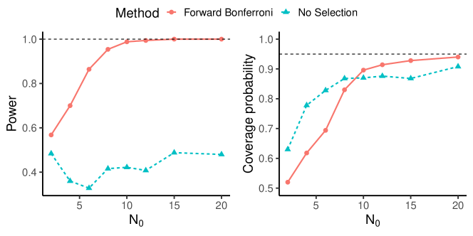
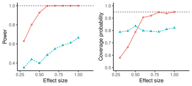
Figure 2: Simulation results on (G1). (i) Top left panel: power curve with varying $N_{0}$; (ii) Top right panel: coverage probability with varying $N_{0}$; (iii) Bottom left panel: power curve with varying effect size $\gamma_{\text{target}}$; (iv) Bottom right panel: coverage probability with varying effect size $\gamma_{\text{target}}$.

Figure 2 demonstrates that the RLS-based estimator ${\widehat{\gamma}}_{\textsc{r}}$ has much higher power than the simple moment estimator ${\widehat{\gamma}}$ for inferring $\gamma_{\text{target}}$ for all considered simulation settings. This echoes our conclusion in Proposition 1 that the RLS-based estimator has reduced variance than the simple moment estimator. Moreover, while the RLS-based estimator attains near nominal coverage probability with reasonably large $N_{0}$ and $\gamma_{\texttt{target}}$, the simple moment estimator tends to provide under-covered confidence intervals in all cases.

7.3 Simulation results for (G2)

In this subsection, we compare the performance of four candidate effect screening methods:

• Forward Bonferroni. Forward screening based on Bonferroni corrected marginal t-tests;

• Forward Lasso. Forward screening based on Lasso;

• Naive Bonferroni. Screening with the full working model based on Bonferroni corrected margin t-tests;

• Naive Lasso. Screening with the full working model based on Lasso.

For each screening method, we evaluate their performance with three measures: (i) perfect screening probability ${\mathbb{P}}\{\widehat{{\mathbb{M}}}={\mathbb{M}}^{\star}\}$, (ii) power of ${\widehat{\gamma}}_{\textsc{r}}$ for testing $\mathrm{H}_{0}:\gamma_{\text{target}}=0$ for the same $\gamma_{\text{target}}$ defined in the previous section, and (iii) coverage probability of the RLS-based confidence interval for $\gamma_{\text{target}}$ with the nominal level at $0.95$. The results are summarized in Figure 3.

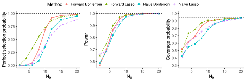
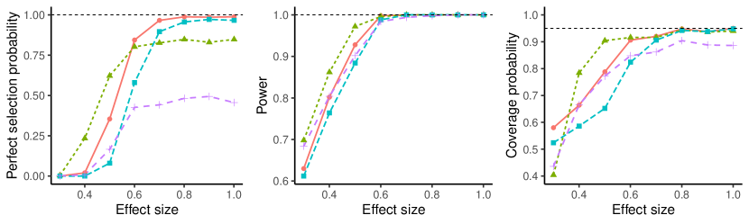
Figure 3: Simulation results on (G2). (i) Top left panel: perfect screening probability with a small fixed effect size $\gamma_{\text{target}}=0.20$ and varying $N_{0}$; (ii) Top middle panel: power curve with a small fixed effect size $\gamma_{\text{target}}=0.20$ and varying $N_{0}$; (iii) Top right panel: coverage probability with a small fixed effect size $\gamma_{\text{target}}=0.20$ and varying $N_{0}$; (iv) Bottom left panel: perfect screening probability with a small fixed replication $N_{0}=2$ and varying effect size $\gamma_{\text{target}}$; (v) Bottom middle panel: power curve with a small fixed replication $N_{0}=2$ and varying effect size $\gamma_{\text{target}}$; (vi) Bottom right panel: coverage probability with a small fixed replication $N_{0}=2$ and varying effect size $\gamma_{\text{target}}$.

From Figure 3, all four effect screening methods lead to perfect selection with high probability as $N_{0}$ or $\gamma_{\texttt{target}}$ increases. Nevertheless, with the forward screening procedure, the probability of perfect screening is higher than the naive screening procedure. Besides, forward screening complies with the heredity structure and demonstrates higher interpretability than the naive screening methods. In terms of the power of ${\widehat{\gamma}}_{\textsc{r}}$ and ${\widehat{v}}_{\textsc{r}}$ for testing $\mathrm{H}_{0}:\gamma_{\text{target}}=0$, while all four methods have power approaching one as $N_{0}$ and $\gamma_{\texttt{target}}$ increases, forward screening based procedures possess higher power with small $N_{0}$ and $\gamma_{\texttt{target}}$. Lastly, we can see an improvement in the coverage probability of the RLS-based confidence intervals with the forward screening procedure.

8 Discussion

In this manuscript, we have discussed the formal theory for forward screening and post-screening inference in $2^{K}$ factorial designs with large $K$. It is conceptually straightforward to extend the theory to general factorial designs with multi-valued factors under more complicated notations, and we thus omit the technical details to simplify the theoretical discussion. Another important direction is covariate adjustment in factorial experiments. Lin (2013), Lu (2016a) and Liu et al. (2022) demonstrated the efficiency gain of covariate adjustment with small $K$. Zhao and Ding (2023) discussed covariate adjustment in factorial experiments with factors and covariates selected independent of data. We leave it to future research to establish the theory for factor screening and covariate selection in factorial designs.

Supplementary material

Section A provides more discussions/extensions to the results introduced in the main paper. More concretely, Section A.1 presents detailed discussion of the use of weight least squares in factorial experiments. Section A.2 extends the inference results in Section 4 to a vector of causal effects.

Section B presents general results on consistency of forward factor screening. Theorem 1 is a corollary of the results in Section B.

Section C gives the technical proofs of the results in the main paper and the Appendix.

Appendix A Additional results

This section provides more extensions to the results in the main paper. Section A.1 discusses the use of WLS in analyzing factorial experiments. Section A.2 extends the inference results under perfect screening (Section 4) to a vector of causal effects.

A.1 Weighted least squares for estimating factorial effects

In this subsection, we briefly state and prove some useful facts about weighted least squares in estimating factorial effects. More discussions can be found in Zhao and Ding (2021). Denote the design matrix as $X=(g_{1,{\mathbb{M}}},\dots,g_{N,{\mathbb{M}}})^{\top}$. Let $W=\mathrm{Diag}\left\{w_{i}\right\}$. The problem (2.6) has closed-form solution:

$${\widehat{\tau}} =(X^{\top}WX)^{-1}(X^{\top}WY)\text{ (closed form solution of WLS)}$$ (S1)

$$=\{G(\cdot,{\mathbb{M}})^{\top}G(\cdot,{\mathbb{M}})\}^{-1}\{G(\cdot,{\mathbb{M}})^{\top}{\widehat{Y}}\}$$ (S2)

(units under the same treatment arm share the same regressor) (S3)

$$=Q^{-1}G(\cdot,{\mathbb{M}})^{\top}{\widehat{Y}}.$$ (S4)

The closed form (S4) motivates the variance estimation:

$${\widehat{V}}_{{\widehat{\tau}}}=Q^{-2}G(\cdot,{\mathbb{M}})^{\top}{\widehat{V}}_{\widehat{Y}}G(\cdot,{\mathbb{M}}).$$ (S5)

Alternatively, one can use the Eicker–Huber–White (EHW) variance estimation with the HC2 correction (Angrist and Pischke, 2009):

$${\widehat{V}}_{\mathrm{EHW}}=(X^{\top}WX)^{-1}X^{\top}W\mathrm{Diag}\left\{\frac{{\widehat{\epsilon}}_{i}^{2}}{1-N_{i}^{-1}}\right\}WX(X^{\top}WX)^{-1},\quad{\widehat{\epsilon}}_{i}=Y_{i}-g_{i,{\mathbb{M}}}^{\top}{\widehat{\tau}}.$$ (S6)

Again, because units under the same treatment arm share the same regressor, ${\widehat{V}}_{\mathrm{EHW}}$ simplifies to

$${\widehat{V}}_{\mathrm{EHW}}=Q^{-2}G(\cdot,{\mathbb{M}})^{\top}{\widehat{V}}^{\prime}_{\widehat{Y}}G(\cdot,{\mathbb{M}}),$$ (S7)

where

$$\quad{\widehat{V}}^{\prime}_{\widehat{Y}}=\mathrm{Diag}\left\{N({\bm{z}})^{-1}{\widehat{S}}^{\prime}({\bm{z}},{\bm{z}})\right\}_{{\bm{z}}\in{\mathcal{T}}}\text{ with }{\widehat{S}}^{\prime}({\bm{z}},{\bm{z}})=\frac{1}{N({\bm{z}})-1}\sum_{Z_{i}={\bm{z}}}(Y_{i}-g_{i,{\mathbb{M}}}^{\top}{\widehat{\tau}})^{2}.$$

Following some algebra, we can show

$${\widehat{S}}^{\prime}({\bm{z}},{\bm{z}}) =\frac{1}{N({\bm{z}})-1}\sum_{Z_{i}={\bm{z}}}(Y_{i}-{\widehat{Y}}({\bm{z}}))^{2}+\frac{N({\bm{z}})}{N({\bm{z}})-1}\{{\widehat{Y}}({\bm{z}})-G({\bm{z}},{\mathbb{M}}){\widehat{\tau}}\}^{2}$$ (S8)

$$={\widehat{S}}({\bm{z}},{\bm{z}})+\frac{N({\bm{z}})}{N({\bm{z}})-1}\{{\widehat{Y}}({\bm{z}})-G({\bm{z}},{\mathbb{M}}){\widehat{\tau}}\}^{2}.$$ (S9)

Hence ${\widehat{S}}^{\prime}({\bm{z}},{\bm{z}})\geq{\widehat{S}}({\bm{z}},{\bm{z}})$. In general ${\widehat{Y}}({\bm{z}})\neq G({\bm{z}},{\mathbb{M}}){\widehat{\tau}}$, so the difference is not negligible. The following Lemma S1 formally summarizes the statistical property of ${\widehat{\tau}}$ and its two variance estimators, ${\widehat{V}}_{\widehat{\tau}}$ and ${\widehat{V}}_{\mathrm{EHW}}$. The proof can be done by utilizing the moment facts from Section C.2 and C.3 of Shi and Ding (2022), which we omit here.

Lemma S1.

Assume Conditions 1 and 3. For the WLS in (2.6), we have

1. ${\widehat{\tau}}=Q^{-1}G(\cdot,{\mathbb{M}})^{\top}{\widehat{Y}}$ is unbiased for the true factorial effects $\tau({\mathbb{M}})$; i.e., ${{\mathbb{E}}\left\{{\widehat{\tau}}\right\}}=\tau({\mathbb{M}})$.

2. Both variance estimators are consistent and robust: $N({\widehat{V}}_{{\widehat{\tau}}}-V_{{\widehat{\tau}},\lim})=o_{\mathbb{P}}(1)$, $N({\widehat{V}}_{\mathrm{EHW}}-V_{\mathrm{EHW},\lim})=o_{\mathbb{P}}(1)$, with $V_{{\widehat{\tau}},\lim}\succcurlyeq V_{{\widehat{\tau}}}$ and $V_{\mathrm{EHW}}\succcurlyeq V_{{\widehat{\tau}}}$, where

   $$V_{{\widehat{\tau}},\lim}=Q^{-2}G(\cdot,{\mathbb{M}})^{\top}D_{\widehat{Y}}G(\cdot,{\mathbb{M}}),$$

   and

   $$V_{\mathrm{EHW},\lim}=Q^{-2}G(\cdot,{\mathbb{M}})^{\top}\mathrm{Diag}\left\{\frac{1-N^{-1}}{N({\bm{z}})-1}S({\bm{z}},{\bm{z}})+\frac{1}{N({\bm{z}})-1}\{\overline{Y}({\bm{z}})-G({\bm{z}},{\mathbb{M}})\tau({\mathbb{M}})\}^{2}\right\}G(\cdot,{\mathbb{M}}).$$

3. EHW variance estimator is more conservative than the direct variance estimator: ${\widehat{V}}_{\mathrm{EHW}}\succcurlyeq{\widehat{V}}_{{\widehat{\tau}}}$.

It is worthy of mentioning that in the fixed $Q$ setting, if we assume that the factorial effects that are not included in ${\mathbb{M}}$ are all zero, Lemma S1 implies EHW variance estimator (S6) or (S7) has the same asymptotic statistical property as the direct variance estimator (S5), which agrees with the conclusion of Zhao and Ding (2021).

A.2 Extension of post-screening inference to vector parameters

In this subsection we present an extension of Theorem 2 to a vector of causal parameters:

$$\Gamma=(\gamma_{1},\dots,\gamma_{L})^{\top},\quad\text{ where }\gamma_{l}={\bm{f}}_{l}^{\top}\overline{Y}.$$

For convenience we can stack ${\bm{f}}_{1},\dots,{\bm{f}}_{L}$ into a weighting matrix $F=({\bm{f}}_{1},\dots,{\bm{f}}_{L})$ and write

$$\Gamma=F^{\top}\overline{Y}.$$ (S10)

We will focus on linear projections of $\Gamma$, defined as $\gamma_{b}=b^{\top}\Gamma$ for a given $b\in{\mathbb{R}}^{L}$. Naturally, we can apply forward screening and construct RLS-based estimators for $\Gamma$:

$${\widehat{\Gamma}}_{\textsc{r}}=({\widehat{\gamma}}_{1,\textsc{r}},\dots,{\widehat{\gamma}}_{L,\textsc{r}})^{\top},\quad{\widehat{V}}_{{\widehat{\Gamma}},\textsc{r}}=F[\widehat{{\mathbb{M}}}]^{\top}{\widehat{V}}_{\widehat{Y}}F[\widehat{{\mathbb{M}}}],$$ (S11)

where

$$F[\widehat{{\mathbb{M}}}]=Q^{-1}G(\cdot,{\widehat{{\mathbb{M}}}})G(\cdot,{\widehat{{\mathbb{M}}}})^{\top}F.$$ (S12)

For $\gamma_{b}$, an estimator based on (S11) is

$${\widehat{\gamma}}_{b,\textsc{r}}=b^{\top}{\widehat{\Gamma}}_{\textsc{r}},\quad{\widehat{v}}^{2}_{b,\textsc{r}}=b^{\top}{\widehat{V}}_{{\widehat{\Gamma}},\textsc{r}}b.$$ (S13)

For standard factorial effects, we can use WLS to obtain the robust covariance matrix (Section A.1). For one single $b$, we can actually apply Theorem 2 with

$${\bm{f}}_{b}=Fb=\sum_{l=1}^{L}b_{l}{\bm{f}}_{l}.$$ (S14)

Define ${\bm{f}}_{b}^{\star}=F[{\mathbb{M}}^{\star}]b$. We then get the following theorem:

Theorem S1 (Statistical properties linear projections of $\Gamma$).

Assume Conditions 1-4. Let $N\to\infty$. Then

$$\frac{{\widehat{\gamma}}_{b,\textsc{r}}-\gamma}{v_{b,\textsc{r}}}\rightsquigarrow{\mathcal{N}}(0,1)$$

where $v^{2}_{b,\textsc{r}}={\bm{f}}_{b}^{\star\top}V_{\widehat{Y}}{\bm{f}}_{b}^{\star}$. Further assume $\|{\bm{f}}_{b}^{\star}\|_{\infty}=O(Q^{-1})$. The variance estimator ${\widehat{v}}_{b,\textsc{r}}^{2}$ is conservative in the sense

$$N({\widehat{v}}_{b,\textsc{r}}^{2}-v_{b,\textsc{r},\mathrm{lim}}^{2})\xrightarrow{{\mathbb{P}}}0,\quad v_{b,\textsc{r},\mathrm{lim}}^{2}\geq v_{b,\textsc{r}}^{2},$$

where $v_{b,\textsc{r},\mathrm{lim}}^{2}={\bm{f}}_{b}^{\star\top}D_{\widehat{Y}}{\bm{f}}_{b}^{\star}$ is the limiting value of ${\widehat{v}}_{b,\textsc{r}}^{2}$.

The proof of Theorem S1 is similar to that of Theorem 2, which is mainly based on Lemma S5 and thus omitted here. Moreover, for a fixed integer $L$, Theorem S1 implies joint normality of ${\widehat{\Gamma}}_{\textsc{r}}$, a result due to the Cramér-Wold theorem. We summarize the result as the following corollary and omit the proof:

Corollary S1.

Assume a fixed $L$. Assume Conditions 1-4. We have

$$V_{{\widehat{\Gamma}},\textsc{r}}^{-1/2}({\widehat{\Gamma}}_{\textsc{r}}-\Gamma)\rightsquigarrow{\mathcal{N}}(0,I_{L}),$$

where $V_{{\widehat{\Gamma}},\textsc{r}}=F[{\mathbb{M}}^{\star}]^{\top}V_{\widehat{Y}}F[{\mathbb{M}}^{\star}]$. Further assume $\max_{\|b\|_{2}=1}\|{\bm{f}}_{b}^{\star}\|_{\infty}=O(Q^{-1})$. The variance estimator ${\widehat{v}}_{b,\textsc{r}}^{2}$ is conservative in the sense that

$$N({\widehat{V}}_{{\widehat{\Gamma}},\textsc{r}}-V_{{\widehat{\Gamma}},\textsc{r},\mathrm{lim}})\xrightarrow{{\mathbb{P}}}0,\quad V_{{\widehat{\Gamma}},\textsc{r},\mathrm{lim}}\succcurlyeq V_{{\widehat{\Gamma}},\textsc{r}},$$

where $V_{{\widehat{\Gamma}},\textsc{r},\mathrm{lim}}=F[{\mathbb{M}}^{\star}]^{\top}D_{\widehat{Y}}F[{\mathbb{M}}^{\star}]^{\top}$ is the limiting value of ${\widehat{V}}_{{\widehat{\Gamma}},\textsc{r}}$.

Appendix B General results on consistency of forward screening

In this section we provide some theoretical insights into the forward factor screening algorithm (Algorithm 1). The discussion in this section starts from a more broad discussion where we allow the S-step to be general procedures that satisfy certain conditions. We will show Bonferroni corrected marginal t-test is a special case of these procedures.

We start with some regularization conditions to characterize a “good” layer-wise S-step, and ensure the P-step is compatible with the structure of the true factorial effects. In light of this, we use ${{\mathbb{M}}}^{\star}_{d,+}$ to denote the pruned set of effects on the $d$-th layer based on the true model ${\mathbb{M}}_{d-1}^{\star}$ on the previous layer; that is,

$${{\mathbb{M}}}^{\star}_{d,+}=\texttt{H}({{\mathbb{M}}}^{\star}_{d-1}).$$

These discussions motivate the following assumption on the layer-wise selection procedure $\widehat{\texttt{S}}(\cdot)$:

Assumption 1 (Validity and consistency of the selection operator).

We denote

$$\widetilde{{\mathbb{M}}}_{d}=\widehat{\text{\em{S}}}({\mathbb{M}}^{\star}_{d,+};\{Y_{i},Z_{i}\}^{N}_{i=1}),$$

where ${\mathbb{M}}^{\star}_{d,+}=\text{\em{H}}({\mathbb{M}}^{\star}_{d-1})$ is defined as above. Let $\{\alpha_{d}\}_{d=1}^{D}$ be a sequence of significance levels in $(0,1)$. We assume that the following validity and consistency property hold for $\text{\em{S}}_{N}(\cdot)$:

$$\text{Validity: }\limsup_{N\to\infty}{\mathbb{P}}\left\{\widetilde{{\mathbb{M}}}_{d}\cap{\mathbb{M}}^{\star c}_{d}\neq\varnothing\right\}\leq\alpha_{d},$$ (S15)

$$\text{Consistency: }\limsup_{N\to\infty}D\sum_{d=1}^{D}{{\mathbb{P}}\left\{\widetilde{{\mathbb{M}}}^{c}_{d}\cap{\mathbb{M}}^{\star}_{d}\neq\varnothing\right\}}=0.$$ (S16)

This assumption can be verified for many screening procedures. In Theorem 1 we will show it holds for the layer-wise Bonferroni corrected marginal testing procedure in Algorithm 1. Moreover, in the high dimensional super population study, a combination of data splitting, adaptation of $\ell_{1}$ regularization and marginal t tests can also fulfill such a requirement (Wasserman and Roeder, 2009).

Besides, we assume the $\texttt{H}(\cdot)$ operator respects the structure of the nonzero factorial effects:

Assumption 2 (H-heredity).

For $d=1,\cdots,D-1$, it holds

$${\mathbb{M}}^{\star}_{d+1}\subset\texttt{\em P}({\mathbb{M}}^{\star}_{d}).$$

One special case of $\texttt{H}(\cdot)$ operator satisfying Assumption 2 is naively adding all the the higher-order interactions regardless of the lower-order screening results. Besides, if we have evidence that the effects have particular hierarchical structure, applying the heredity principles can improve screening accuracy as well as interpretability of the screening results.

Theorem S2 (Screening consistency).

Assume Assumption 1 and 2. Then the forward screening procedure (3.8) has the following properties:

1. Type I error control. Forward screening controls the Type I error rate, in the sense that

   $$\underset{N\to\infty}{\lim\sup}~{}{\mathbb{P}}\left(\widehat{{\mathbb{M}}}_{d}\cap{{\mathbb{M}}_{d}^{\star}}^{c}\neq\varnothing\text{ for some }d\in[D]\right)\leq\alpha=\sum_{d=1}^{D}\alpha_{d}.$$ (S17)

2. Screening consistency. Further assume $\alpha=\alpha_{N}\to 0$. The forward procedure consistently selects all the nonzero effects up to $D$ levels with probability tending to 1:

   $$\underset{N\to\infty}{\lim\sup}~{}{\mathbb{P}}\left(\widehat{{\mathbb{M}}}_{d}={\mathbb{M}}_{d}^{\star}\text{ for all }d\in[D]\right)=1.$$ (S18)

Theorem S2 consists of two parts. First, one can control the type I error rate, which is defined as the probability of over-selects at least one zero effect. The definition is introduced and elaborated detailedly in Wasserman and Roeder (2009) for model selection. Second, if the tuning parameter $\alpha=\sum_{d=1}^{D}\alpha_{d}$ vanish asymptotically, one can actually achieve perfect screening up to $D$ levels of effects. To apply Theorem S2 to specific procedures, the key step is to verify Assumption 1 and justify Assumption 2, which we will do for Bonferroni corrected marginal t tests as an example in the next section.

Moreover, the scaling of $\alpha_{N}$ plays an important role in theoretical discussion. To achieve perfect selection, we hope $\alpha_{N}$ decays as fast as possible; ideally if $\alpha_{N}$ equals zero then we do not commit any type I error (or equivalently, we will never select redundant effects). However, for many data-dependent selection procedure $\alpha$ can only decay at certain rates, because a fast decaying $\alpha$ means higher possibility of rejection, thus can lead to strict under-selection. Therefore, in the tuning process, $\alpha_{d}$ should be scaled properly if one wants to pursue perfect selection. Nevertheless, even if the tuning is hard and perfect model selection can not be achieved, we still have many strategies to exploit the advantage of the forward screening procedure. We will have more discussions in later sections.

Lastly, as we have commented earlier, in practice people have many alternative methods for the S-step. They are attractive in factorial experiments because many lead to simple form solutions due to the orthogonality of factorial designs. For example, Lasso is a commonly adopted strategy for variable selection in linear models (Zhao and Yu, 2006). It solves the following penalized WLS problem in factorial settings:

$$\widehat{{\mathbb{M}}}_{\textsc{l}}=\{{\mathcal{K}}:{\widehat{\tau}}_{\textsc{l},{\mathcal{K}}}\neq 0\},\quad{\widehat{\tau}}_{\textsc{l},{\mathcal{K}}}=\min_{\tau^{\prime}\in\mathbb{R}^{H}}\frac{1}{2}\sum_{{\bm{z}}\in{\mathcal{T}}}w_{i}(Y_{i}-g_{i}^{\top}\tau^{\prime})^{2}+\lambda_{\textsc{l}}\|\tau^{\prime}\|_{1}.$$

Due to the orthogonality of $G$, the resulting $\widehat{{\mathbb{M}}}$ has a closed-form solution (Hastie et al., 2009):

$$\widehat{{\mathbb{M}}}_{\textsc{l}}=\{{\mathcal{K}}:|{\widehat{\tau}}_{{\mathcal{K}}}|\geq\lambda_{\textsc{l}}\}.$$ (S19)

Other methods, such as AIC/BIC (Bai et al., 2022), sure independence screening (Fan and Lv, 2008), etc., are also applicable. With more delicate assumptions and tuning parameter choices, these methods can also be justified theoretically for screening consistency and post-screening inference. We omit the details.

Appendix C Technical proofs

In this section we present the technical proofs for the results across the whole paper. Section C.1 presents some preliminary probabilistic results that are useful in randomized experiments which are mainly attributed to Shi and Ding (2022). The main proof starts from Section C.2.

C.1 Preliminaries: some important probabilistic results in randomized experiments

In this subsection we present some preliminary probability results that are crucial for our theoretical discussion. Consider an estimator of the form

$${\widehat{\gamma}}=Q^{-1}\sum_{{\bm{z}}\in{\mathcal{T}}}w({\bm{z}})\widehat{Y}({\bm{z}}),$$

with variance estimator

$$\widehat{v}^{2}=Q^{-2}\sum_{{\bm{z}}\in{\mathcal{T}}}w({\bm{z}})^{2}\widehat{S}({\bm{z}},{\bm{z}}).$$

Li and Ding (2017) showed that

$${\mathbb{E}}\{{\widehat{Y}}\}=\overline{Y},~{}V_{\widehat{Y}}={\operatorname{Var}\left\{{\widehat{Y}}\right\}}=D_{\widehat{Y}}-N^{-1}S.$$ (S20)

Then (S20) further leads to the following facts:

$${\mathbb{E}}\{{\widehat{\gamma}}\} =\sum_{{\bm{z}}\in{\mathcal{T}}}{\bm{f}}({\bm{z}})\overline{Y}({\bm{z}})=\gamma,$$ (S21)

$${\operatorname{Var}\left\{{\widehat{\gamma}}\right\}} =\sum_{{\bm{z}}\in{\mathcal{T}}}{\bm{f}}({\bm{z}})^{2}N({{\bm{z}}})^{-1}S({\bm{z}},{\bm{z}})-N^{-1}{\bm{f}}^{\top}S{\bm{f}},$$ (S22)

$${\mathbb{E}}\{\widehat{v}^{2}\} =\sum_{{\bm{z}}\in{\mathcal{T}}}{\bm{f}}({\bm{z}})^{2}N({{\bm{z}}})^{-1}S({\bm{z}},{\bm{z}}).$$ (S23)

We have the following variance estimation results and Berry–Esseen bounds:

Lemma S2 (Variance concentration and Berry–Esseen bounds in finite population).

Define $\gamma={\mathbb{E}}\{{\widehat{\gamma}}\}$, $v^{2}=\operatorname{Var}({\widehat{\gamma}})$ and $v^{2}_{\lim}={\mathbb{E}}\{\widehat{v}^{2}\}$. Suppose the following conditions hold:

• Nondegenerate variance. There exists a $\sigma_{w}>0$, such that

  $$Q^{-2}\sum_{{\bm{z}}=1}^{Q}w({\bm{z}})^{2}N_{{\bm{z}}}^{-1}S({\bm{z}},{\bm{z}})\leq\sigma_{w}^{2}v^{2}.$$ (S24)

• Bounded fourth moments. There exists a $\delta>0$ such that

  $$\max_{{\bm{z}}\in[Q]}\frac{1}{N}\sum_{i=1}^{N}\{Y_{i}({\bm{z}})-\overline{Y}({\bm{z}})\}^{4}\leq\Delta^{4}.$$ (S25)

Then we have the following conclusions:

1. The variance estimator is conservative for the true variance: $v^{2}_{\lim}\geq v^{2}$. Besides, the following tail bound holds:

   $${\mathbb{P}}\left\{N|\widehat{v}^{2}-v^{2}_{\lim}|>t\right\}\leq\frac{C\overline{c}^{3}\underline{c}^{-4}\|w\|_{\infty}^{2}\Delta^{4}}{QN_{0}}\cdot\frac{1}{t^{2}}.$$ (S26)

2. We have a Berry–Esseen bound with the true variance:

   $$\sup_{t\in{\mathbb{R}}}\left|{{\mathbb{P}}\left\{\frac{{\widehat{\gamma}}-\gamma}{v}\leq t\right\}}-\Phi(t)\right|\leq 2C\sigma_{w}\frac{\underline{c}^{-1}\|w\|_{\infty}\max_{i\in[N],{\bm{z}}\in[Q]}|Y_{i}({\bm{z}})-\overline{Y}({\bm{z}})|}{\|w\|_{2}\sqrt{\overline{c}^{-1}\min_{{\bm{z}}\in[Q]}S({\bm{z}},{\bm{z}})}\cdot\sqrt{N_{0}}}.$$ (S27)

3. We have a Berry–Esseen bound with the estimated variance: for any $\epsilon_{N}\in(0,1/2]$,

   $$\sup_{t\in{\mathbb{R}}}\left|{\mathbb{P}}\left\{\frac{{\widehat{\gamma}}-\gamma}{\widehat{v}}\leq t\right\}-\Phi\left(\frac{v_{\lim}}{v}t\right)\right| \leq\epsilon_{N}+\frac{C\overline{c}^{3}\underline{c}^{-4}\|w\|_{\infty}^{2}\Delta^{4}}{QN_{0}}\cdot\frac{1}{(Nv^{2}\epsilon_{N})^{2}}$$

   $$+2C\sigma_{w}\frac{\underline{c}^{-1}\|w\|_{\infty}\max_{i\in[N],{\bm{z}}\in[Q]}|Y_{i}({\bm{z}})-\overline{Y}({\bm{z}})|}{\|w\|_{2}\sqrt{\overline{c}^{-1}\min_{{\bm{z}}\in[Q]}S({\bm{z}},{\bm{z}})}\cdot\sqrt{N_{0}}}.$$

Proof of Lemma S2.

1. See Lemma S13 of Shi and Ding (2022).

2. See Theorem 1 of Shi and Ding (2022).

3. First we show a useful result: for $|a|\leq 1/2$ and any $b\in{\mathbb{R}}$,

   $$\sup_{t\in{\mathbb{R}}}|\Phi\{(1+a)t+b\}-\Phi\{t\}|\leq|a|+|b|.$$ (S28)

   (S28) is particularly useful for small choices of $a$ and $b$. Intuitively, it evaluates the change of $\Phi$ under a small affine perturbation of $t$.

   The proof of (S28) is based on a simple step of the mean value theorem: for any $t\in{\mathbb{R}}$,

   $$|\Phi\{(1+a)t+b\}-\Phi\{t\}|$$

   $$= |\phi(\xi_{t,(1+a)t})\cdot(at+b)|$$

   $$= |\phi(\xi_{t,(1+a)t})\cdot at|+|\phi(\xi_{t,(1+a)t})\cdot b|$$

   $$= |a|\cdot|\phi(\xi_{t,(1+a)t})\cdot t|\cdot\bm{1}\left\{|t|\leq 1\right\}+|a|\cdot|\phi(\xi_{t,(1+a)t})\cdot t|\cdot\bm{1}\left\{|t|>1\right\}+|\phi(\xi_{t,(1+a)t})\cdot b|$$

   $$\leq \frac{1}{\sqrt{2\pi}}|a|\cdot\bm{1}\left\{|t|\leq 1\right\}+\frac{1}{\sqrt{2\pi}}|a||t|\cdot\exp(-t^{2}/8)\cdot\bm{1}\left\{|t|>1\right\}+{\frac{1}{\sqrt{2\pi}}}|b|$$

   $$\leq |a|+|b|.$$

   We consider $t\geq 0$ because $t<0$ can be handled similarly. For any $\epsilon_{N}>0$, We have

   $${\mathbb{P}}\left\{\frac{{\widehat{\gamma}}-\gamma}{\widehat{v}}\leq t\right\} ={\mathbb{P}}\left\{\frac{{\widehat{\gamma}}-\gamma}{{v}}\leq\frac{\widehat{v}}{{v}}t\right\}$$

   $$={\mathbb{P}}\left\{\frac{{\widehat{\gamma}}-\gamma}{{v}}\leq\frac{\widehat{v}}{{v}}t,\left|\frac{\widehat{v}-v_{\lim}}{v}\right|\leq\epsilon_{N}\right\}+{\mathbb{P}}\left\{\frac{{\widehat{\gamma}}-\gamma}{{v}}\leq\frac{\widehat{v}}{{v}}t,\left|\frac{\widehat{v}-v_{\lim}}{v}\right|>\epsilon_{N}\right\}.$$

   Then we can show that

   $${\mathbb{P}}\left\{\frac{{\widehat{\gamma}}-\gamma}{\widehat{v}}\leq t\right\} \leq{\mathbb{P}}\left\{\frac{{\widehat{\gamma}}-\gamma}{{v}}\leq\frac{\widehat{v}}{{v}}t,\left|\frac{\widehat{v}-v_{\lim}}{v}\right|\leq\epsilon_{N}\right\}+{\mathbb{P}}\left\{\left|\frac{\widehat{v}-v_{\lim}}{v}\right|>\epsilon_{N}\right\}$$

   $$\leq{\mathbb{P}}\left\{\frac{{\widehat{\gamma}}-\gamma}{{v}}\leq\left(\frac{{v}}{v}+\epsilon_{N}\right)t\right\}+{\mathbb{P}}\left\{\left|\frac{\widehat{v}-v_{\lim}}{v}\right|>\epsilon_{N}\right\}.$$

   For the first term, we have

   $$\sup_{t\geq 0}\left|{\mathbb{P}}\left\{\frac{{\widehat{\gamma}}-\gamma}{{v}}\leq\left(\frac{{v}_{\lim}}{v}+\epsilon_{N}\right)t\right\}-\Phi\left\{\left(\frac{{v}_{\lim}}{v}+\epsilon_{N}\right)t\right\}\right|$$

   $$\leq 2C\sigma_{w}\frac{\underline{c}^{-1}\|w\|_{\infty}\max_{i\in[N],{\bm{z}}\in[Q]}|Y_{i}({\bm{z}})-\overline{Y}({\bm{z}})|}{\|w\|_{2}\sqrt{\overline{c}^{-1}\min_{{\bm{z}}\in[Q]}S({\bm{z}},{\bm{z}})}\cdot\sqrt{N_{0}}}.$$

   For the second term, using the variance estimation results in Part 1 we have

   $${\mathbb{P}}\left\{\left|\frac{\widehat{v}-v_{\lim}}{v}\right|\geq\epsilon_{N}\right\} \leq{\mathbb{P}}\left\{\left|\frac{\widehat{v}-v_{\lim}}{v}\right|\cdot\left|\frac{\widehat{v}+v_{\lim}}{v}\right|\geq\epsilon_{N}\right\}\text{ (because $v_{\lim}$ is conservative)}$$

   $$={\mathbb{P}}\left\{\left|\frac{N\widehat{v}^{2}-Nv^{2}_{\lim}}{Nv^{2}}\right|\geq\epsilon_{N}\right\}$$

   $$\leq\frac{C\overline{c}^{3}\underline{c}^{-4}\|w\|_{\infty}^{2}\Delta^{4}}{QN_{0}}\cdot\frac{1}{(Nv^{2}\epsilon_{N})^{2}}.$$

   Besides, by (S28), when $\epsilon_{N}\leq 1/2$, we also have

   $$\sup_{t\in{\mathbb{R}}}\left|\Phi\left\{\left(\frac{{v}_{\lim}}{v}+\epsilon_{N}\right)t\right\}-\Phi\left(\frac{v_{\lim}}{v}t\right)\right|\leq\frac{v\epsilon_{N}}{v_{\lim}}\leq\epsilon_{N}.$$

   Aggregating all the parts above, we can show that for any $t\geq 0$,

   $${\mathbb{P}}\left\{\frac{{\widehat{\gamma}}-\gamma}{\widehat{v}}\leq t\right\} \leq\Phi\left(\frac{v_{\lim}}{v}t\right)+\epsilon_{N}+\frac{C\overline{c}^{3}\underline{c}^{-4}\|w\|_{\infty}^{2}\Delta^{4}}{QN_{0}}\cdot\frac{1}{(Nv^{2}\epsilon_{N})^{2}}$$

   $$+2C\sigma_{w}\frac{\underline{c}^{-1}\|w\|_{\infty}\max_{i\in[N],{\bm{z}}\in[Q]}|Y_{i}({\bm{z}})-\overline{Y}({\bm{z}})|}{\|w\|_{2}\sqrt{\overline{c}^{-1}\min_{{\bm{z}}\in[Q]}S({\bm{z}},{\bm{z}})}\cdot\sqrt{N_{0}}}.$$

   On the other hand, we can show that

   $${\mathbb{P}}\left\{\frac{{\widehat{\gamma}}-\gamma}{\widehat{v}}\leq t\right\} \geq{\mathbb{P}}\left\{\frac{{\widehat{\gamma}}-\gamma}{{v}}\leq\frac{\widehat{v}}{{v}}t,\left|\frac{\widehat{v}-v_{\lim}}{v}\right|\leq\epsilon_{N}\right\}$$

   $$\geq{\mathbb{P}}\left\{\frac{{\widehat{\gamma}}-\gamma}{{v}}\leq\left(\frac{{v}_{\lim}}{v}-\epsilon_{N}\right)t\right\}-{\mathbb{P}}\left\{\left|\frac{\widehat{v}-v_{\lim}}{v}\right|\geq\epsilon_{N}\right\}.$$ (S29)

   By (S28), when $\epsilon_{N}\leq 1/2$, we also have

   $$\sup_{t\in{\mathbb{R}}}\left|\Phi\left\{\left(\frac{{v}_{\lim}}{v}-\epsilon_{N}\right)t\right\}-\Phi\left(\frac{v_{\lim}}{v}t\right)\right|\leq\epsilon_{N}.$$

   So we can derive a lower bound analogous to (S29). Note that the results can be analogously generalized to $t\leq 0$. Putting pieces together, we can show that for any $t\geq 0$,

   $$\sup_{t\in{\mathbb{R}}}\left|{\mathbb{P}}\left\{\frac{{\widehat{\gamma}}-\gamma}{\widehat{v}}\leq t\right\}-\Phi\left(\frac{v_{\lim}}{v}t\right)\right| \leq\epsilon_{N}+\frac{C\overline{c}^{3}\underline{c}^{-4}\|w\|_{\infty}^{2}\Delta^{4}}{QN_{0}}\cdot\frac{1}{(Nv^{2}\epsilon_{N})^{2}}$$

   $$+2C\sigma_{w}\frac{\underline{c}^{-1}\|w\|_{\infty}\max_{i\in[N],{\bm{z}}\in[Q]}|Y_{i}({\bm{z}})-\overline{Y}({\bm{z}})|}{\|w\|_{2}\sqrt{\overline{c}^{-1}\min_{{\bm{z}}\in[Q]}S({\bm{z}},{\bm{z}})}\cdot\sqrt{N_{0}}}.$$

∎

The following corollary shows a Berry–Esseen bound for the studentized statistic in the special case where $w=(w({\bm{z}}))_{{\bm{z}}\in[Q]}$ is a contrast vector for factorial effects. That is, $w=g_{\mathcal{K}}$ for some ${\mathcal{K}}\in{\mathbb{K}}$.

Corollary S2.

Assume Condition (S24) and (S25) hold. Let $w=g_{\mathcal{K}}$ for some ${\mathcal{K}}\in{\mathbb{K}}$. Then we have a Berry–Esseen bound with the estimated variance:

$$\sup_{t\in{\mathbb{R}}}\left|{\mathbb{P}}\left\{\frac{{\widehat{\tau}}_{\mathcal{K}}-\tau_{\mathcal{K}}}{\widehat{v}}\leq t\right\}-\Phi\left(\frac{v_{\lim}}{v}t\right)\right| \leq 2\left(\frac{C\sigma_{w}^{4}\overline{c}^{5}\underline{c}^{-6}\Delta^{4}}{\{\min_{{\bm{z}}\in{\mathcal{T}}}S({\bm{z}},{\bm{z}})\}^{2}}\right)^{1/3}\cdot\frac{1}{(QN_{0})^{1/3}}$$

$$+2C\sigma_{w}\frac{\underline{c}^{-1}\max_{i\in[N],{\bm{z}}\in[Q]}|Y_{i}({\bm{z}})-\overline{Y}({\bm{z}})|}{\sqrt{\overline{c}^{-1}\min_{{\bm{z}}\in[Q]}S({\bm{z}},{\bm{z}})}}\cdot\frac{1}{(QN_{0})^{1/2}}.$$

Proof of Corollary S2.

Lower bound for $Nv^{2}$. Note that $\|w\|_{2}^{2}=Q$ and $\|w\|_{\infty}=1$. Using Condition (S24), we have

$$Nv^{2} \geq N\sigma_{w}^{-2}Q^{-2}\sum_{{\bm{z}}=1}^{Q}w({\bm{z}})^{2}N_{{\bm{z}}}^{-1}S({\bm{z}},{\bm{z}})$$

$$\geq(\underline{c}QN_{0})\cdot\sigma_{w}^{-2}\overline{c}^{-1}Q^{-1}N_{0}^{-1}\min_{{\bm{z}}\in{\mathcal{T}}}S({\bm{z}},{\bm{z}})\cdot(Q^{-1}\|w\|_{2}^{2})$$

$$=\sigma_{w}^{-2}\underline{c}\overline{c}^{-1}\min_{{\bm{z}}\in{\mathcal{T}}}S({\bm{z}},{\bm{z}}).$$

Therefore, the Berry–Esseen bound becomes

$$\sup_{t\in{\mathbb{R}}}\left|{\mathbb{P}}\left\{\frac{{\widehat{\tau}}_{\mathcal{K}}-\tau_{\mathcal{K}}}{\widehat{v}}\leq t\right\}-\Phi\left(\frac{v_{\lim}}{v}t\right)\right| \leq\epsilon_{N}+\frac{C\sigma_{w}^{4}\overline{c}^{5}\underline{c}^{-6}\Delta^{4}}{(QN_{0})\{\min_{{\bm{z}}\in{\mathcal{T}}}S({\bm{z}},{\bm{z}})\}^{2}}\cdot\frac{1}{\epsilon_{N}^{2}}$$

$$+2C\sigma_{w}\frac{\underline{c}^{-1}\max_{i\in[N],{\bm{z}}\in[Q]}|Y_{i}({\bm{z}})-\overline{Y}({\bm{z}})|}{\sqrt{\overline{c}^{-1}\min_{{\bm{z}}\in[Q]}S({\bm{z}},{\bm{z}})}\cdot\sqrt{QN_{0}}}.$$

Optimize the summation of the first and second term. By taking derivative over $\epsilon_{N}$ on the upper bound and solving for the zero point, we know that when

$$\epsilon_{N}=\left(\frac{2C\sigma_{w}^{4}\overline{c}^{5}\underline{c}^{-6}\Delta^{4}}{(QN_{0})\{\min_{{\bm{z}}\in{\mathcal{T}}}S({\bm{z}},{\bm{z}})\}^{2}}\right)^{1/3},$$

the upper bound is minimized and

$$\sup_{t\in{\mathbb{R}}}\left|{\mathbb{P}}\left\{\frac{{\widehat{\tau}}_{\mathcal{K}}-\tau_{\mathcal{K}}}{\widehat{v}}\leq t\right\}-\Phi\left(\frac{v_{\lim}}{v}t\right)\right| \leq 2\left(\frac{C\sigma_{w}^{4}\overline{c}^{5}\underline{c}^{-6}\Delta^{4}}{\{\min_{{\bm{z}}\in{\mathcal{T}}}S({\bm{z}},{\bm{z}})\}^{2}}\right)^{1/3}\cdot\frac{1}{(QN_{0})^{1/3}}$$

$$+2C\sigma_{w}\frac{\underline{c}^{-1}\max_{i\in[N],{\bm{z}}\in[Q]}|Y_{i}({\bm{z}})-\overline{Y}({\bm{z}})|}{\sqrt{\overline{c}^{-1}\min_{{\bm{z}}\in[Q]}S({\bm{z}},{\bm{z}})}}\cdot\frac{1}{(QN_{0})^{1/2}}.$$

∎

Additionally, we have a Berry–Esseen bounds after screening the effects:

Lemma S3 (Berry Esseen bound with screening).

Assume there exists $\sigma_{w}>0$ such that

$$\sum_{{\bm{z}}=1}^{Q}{{\bm{f}}}[{\mathbb{M}}]({\bm{z}})^{2}N_{{\bm{z}}}^{-1}S({\bm{z}},{\bm{z}})\leq\sigma_{w}^{2}v^{2}({\mathbb{M}}).$$ (S30)

Then

$$\sup_{t\in{\mathbb{R}}}\left|{{\mathbb{P}}\left\{\frac{{\widehat{\gamma}}[\widehat{{\mathbb{M}}}]-\gamma[{\mathbb{M}}]}{v({\mathbb{M}})}\leq t\right\}}-\Phi(t)\right|$$

$$\leq 2{{\mathbb{P}}\left\{\widehat{{\mathbb{M}}}\neq{\mathbb{M}}\right\}}+2C\sigma_{w}\frac{\underline{c}^{-1}\max_{i\in[N],{\bm{z}}\in[Q]}|Y_{i}({\bm{z}})-\overline{Y}({\bm{z}})|}{\sqrt{\overline{c}^{-1}\min_{{\bm{z}}\in[Q]}S({\bm{z}},{\bm{z}})}\cdot\sqrt{N_{0}}}\cdot\frac{\|{{\bm{f}}}[{\mathbb{M}}]\|_{\infty}}{\|{{\bm{f}}}[{\mathbb{M}}]\|_{2}}.$$ (S31)

Proof of Lemma S3.

With the selected working model we have

$$\sup_{t\in{\mathbb{R}}}\left|{{\mathbb{P}}\left\{\frac{{\widehat{\gamma}}[\widehat{{\mathbb{M}}}]-\gamma[{\mathbb{M}}]}{v({\mathbb{M}})}\leq t\right\}}-\Phi(t)\right|$$

$$= \sup_{t\in{\mathbb{R}}}\left|{{\mathbb{P}}\left\{\frac{{\widehat{\gamma}}[\widehat{{\mathbb{M}}}]-\gamma[{\mathbb{M}}]}{v({\mathbb{M}})}\leq t,\widehat{{\mathbb{M}}}={\mathbb{M}}\right\}}-\Phi(t)+{{\mathbb{P}}\left\{\frac{{\widehat{\gamma}}[\widehat{{\mathbb{M}}}]-\gamma[{\mathbb{M}}]}{v({\mathbb{M}})}\leq t,\widehat{{\mathbb{M}}}\neq{\mathbb{M}}\right\}}\right|$$

$$\leq \sup_{t\in{\mathbb{R}}}\left|{{\mathbb{P}}\left\{\frac{{\widehat{\gamma}}[\widehat{{\mathbb{M}}}]-\gamma[{\mathbb{M}}]}{v({\mathbb{M}})}\leq t,\widehat{{\mathbb{M}}}={\mathbb{M}}\right\}}-\Phi(t)\right|+{{\mathbb{P}}\left\{\frac{{\widehat{\gamma}}[\widehat{{\mathbb{M}}}]-\gamma[{\mathbb{M}}]}{v({\mathbb{M}})}\leq t,\widehat{{\mathbb{M}}}\neq{\mathbb{M}}\right\}}$$

$$= \sup_{t\in{\mathbb{R}}}\left|{{\mathbb{P}}\left\{\frac{{\widehat{\gamma}}[{{\mathbb{M}}}]-\gamma[{\mathbb{M}}]}{v({\mathbb{M}})}\leq t,\widehat{{\mathbb{M}}}={\mathbb{M}}\right\}}-\Phi(t)\right|+{{\mathbb{P}}\left\{\frac{{\widehat{\gamma}}[\widehat{{\mathbb{M}}}]-\gamma[{\mathbb{M}}]}{v({\mathbb{M}})}\leq t,\widehat{{\mathbb{M}}}\neq{\mathbb{M}}\right\}}$$

$$\leq \sup_{t\in{\mathbb{R}}}\left|{{\mathbb{P}}\left\{\frac{{\widehat{\gamma}}[{{\mathbb{M}}}]-\gamma[{\mathbb{M}}]}{v({\mathbb{M}})}\leq t\right\}}-\Phi(t)\right|+2{{\mathbb{P}}\left\{\widehat{{\mathbb{M}}}\neq{\mathbb{M}}\right\}}.$$

Now we have

$${\widehat{\gamma}}({\mathbb{M}}) ={\bm{f}}^{\top}G(\cdot,{\mathbb{M}}){\widehat{\tau}}({\mathbb{M}})$$

$$={\bm{f}}^{\top}G(\cdot,{\mathbb{M}})G(\cdot,{\mathbb{M}})^{\top}{\widehat{Y}}$$

$$={{\bm{f}}}[{\mathbb{M}}]^{\top}{\widehat{Y}}.$$

By Theorem 1 of Shi and Ding (2022), we have a Berry–Esseen bound with the true variance:

$$\sup_{t\in{\mathbb{R}}}\left|{{\mathbb{P}}\left\{\frac{{\widehat{\gamma}}({{\mathbb{M}}})-\gamma[{\mathbb{M}}]}{v}\leq t\right\}}-\Phi(t)\right|\leq 2C\sigma_{w}\frac{\|{{\bm{f}}}[{\mathbb{M}}]\|_{\infty}\underline{c}^{-1}\max_{i\in[N],{\bm{z}}\in[Q]}|Y_{i}({\bm{z}})-\overline{Y}({\bm{z}})|}{\|{{\bm{f}}}[{\mathbb{M}}]\|_{2}\sqrt{\overline{c}^{-1}\min_{{\bm{z}}\in[Q]}S({\bm{z}},{\bm{z}})}\cdot\sqrt{N_{0}}}.$$

∎

A crucial quantity that appeared in Lemma S3 is the ratio of norms:

$$\frac{\|{{\bm{f}}}[{\mathbb{M}}]\|_{\infty}}{\|{{\bm{f}}}[{\mathbb{M}}]\|_{2}}.$$ (S32)

The following Lemma S4 provides an explicit bound on (S32) which reveals how the ratio is controlled with respect to the size of the working model.

Lemma S4.

For ${\bm{f}}[{\mathbb{M}}]\neq 0$, we have

$$\frac{\|{\bm{f}}[{\mathbb{M}}]\|_{\infty}}{\|{\bm{f}}[{\mathbb{M}}]\|_{2}}\leq\left(\frac{|{\mathbb{M}}|}{Q}\right)^{1/2}.$$ (S33)

Proof of Lemma S4.

Because the LHS of (S33) is a ratio, based on the definition of ${\bm{f}}^{\star}$ (4.14) we can assume $\|{\bm{f}}\|_{2}=1$ without loss of generality. Due to the orthogonality of $G$, we can use the columns of $G$ as bases and express ${\bm{f}}$ as

$${\bm{f}}=\frac{1}{\sqrt{Q}}G(\cdot,{\mathbb{M}})b_{1}+\frac{1}{\sqrt{Q}}G(\cdot,{\mathbb{M}}^{c})b_{2},$$

where $b_{1}\in{\mathbb{R}}^{|{\mathbb{M}}|}$ and $b_{2}\in{\mathbb{R}}^{|{\mathbb{M}}^{c}|}$ and $\|(b_{1}^{\top},b_{2}^{\top})^{\top}\|_{2}=1$. Then

$${\bm{f}}[{\mathbb{M}}]=Q^{-1}G(\cdot,{\mathbb{M}})G(\cdot,{\mathbb{M}})^{\top}{\bm{f}}=\frac{1}{\sqrt{Q}}G(\cdot,{\mathbb{M}})b_{1}.$$

Hence

$$\|{\bm{f}}[{\mathbb{M}}]\|_{\infty}\leq\frac{1}{\sqrt{Q}}\|b_{1}\|_{1},\quad\|{\bm{f}}[{\mathbb{M}}]\|_{2}=\|b_{1}\|_{2},\quad\frac{\|{\bm{f}}[{\mathbb{M}}]\|_{\infty}}{\|{\bm{f}}[{\mathbb{M}}]\|_{2}}\leq\frac{1}{\sqrt{Q}}\cdot\frac{\|b_{1}\|_{1}}{\|b_{1}\|_{2}}\leq\left(\frac{|{\bm{f}}[{\mathbb{M}}]|}{Q}\right)^{1/2}.$$

∎

C.2 Proof of Theorem S2

Proof of Theorem S2.

According to the orthogonality of designs, the signs for all terms in the studied unsaturated population regressions are consistent with those of saturated regressions, which saves the effort of differentiating true models for partial and full regression. We introduce several key events that will play a crucial role in the proof: for $D_{0}\in[D]$, define

$$\textit{Under-selection: }{\mathcal{E}}_{\textsc{u}}(D_{0})=\{\widehat{{\mathbb{M}}}_{d}\subset{\mathbb{M}}^{\star}_{d},d\in[D_{0}]\},$$ (S34)

$$\textit{Strict under-selection: }{\mathcal{E}}_{\textsc{su}}(D_{0})=\{\widehat{{\mathbb{M}}}_{d}\subset{\mathbb{M}}^{\star}_{d},d\in[D_{0}];\text{ there exists }d\in[D_{0}],\widehat{{\mathbb{M}}}_{d}\subsetneq{\mathbb{M}}^{\star}_{d}\}.$$ (S35)

High level idea of the proof. To prove screening consistency, we will prove two facts:

$${{\mathbb{P}}\left\{{\mathcal{E}}_{\textsc{u}}(D)\text{ holds}\right\}}\to 1,\quad{{\mathbb{P}}\left\{{\mathcal{E}}_{\textsc{su}}(D)\text{ holds}\right\}}\to 0.$$ (S36)

Combining these two results together, we can conclude asymptotic screening consistency.

We start from the strict under-selection probability.

Step 1: Prove that asymptotically, there is no strict under-selection.

By definition,

$${{\mathbb{P}}\left\{{\mathcal{E}}_{\textsc{su}}(1)\text{ holds}\right\}}={{\mathbb{P}}\left\{\widetilde{{\mathbb{M}}}_{1}\subsetneq{\mathbb{M}}^{\star}_{1}\right\}}\leq{{\mathbb{P}}\left\{\widetilde{{\mathbb{M}}}_{1}^{c}\cap{{\mathbb{M}}_{1}^{\star}}\neq\varnothing\right\}}.$$

We now derive a recursive bound for ${{\mathbb{P}}\left\{{\mathcal{E}}_{\textsc{su}}(D_{0}+1)\text{ holds}\right\}}$ where $1\leq D_{0}\leq D-1$. We have decomposition

$${\mathcal{E}}_{\textsc{su}}(D_{0}+1) =\left\{\widehat{{\mathbb{M}}}_{d}\subset{\mathbb{M}}^{\star}_{d},d\leq D_{0}+1\right\}-\left\{\widehat{{\mathbb{M}}}_{d}={\mathbb{M}}^{\star}_{d},d\leq D_{0}+1\right\}$$

$$={\mathcal{E}}_{\textsc{su,1}}(D_{0}+1)\cup{\mathcal{E}}_{\textsc{su,2}}(D_{0}+1),$$

where

$${\mathcal{E}}_{\textsc{su,1}}(D_{0}+1)=\left\{\widehat{{\mathbb{M}}}_{d}\subset{\mathbb{M}}^{\star}_{d},d\leq D_{0}+1\right\}-\left\{\widehat{{\mathbb{M}}}_{d}={\mathbb{M}}^{\star}_{d},d\leq D_{0};\widehat{{\mathbb{M}}}_{D_{0}+1}\subset{\mathbb{M}}^{\star}_{D_{0}+1}\right\},$$ (S37)

$${\mathcal{E}}_{\textsc{su,2}}(D_{0}+1)=\left\{\widehat{{\mathbb{M}}}_{d}={\mathbb{M}}^{\star}_{d},d\leq D_{0};\widehat{{\mathbb{M}}}_{D_{0}+1}\subset{\mathbb{M}}^{\star}_{D_{0}+1}\right\}-\left\{\widehat{{\mathbb{M}}}_{d}={\mathbb{M}}^{\star}_{d},d\leq D_{0}+1\right\}.$$ (S38)

For ${\mathcal{E}}_{\textsc{su,1}}(D_{0}+1)$, we have

$${{\mathbb{P}}\left\{{\mathcal{E}}_{\textsc{su,1}}(D_{0}+1)\text{ holds}\right\}} ={\mathbb{P}}\left(\left\{\widehat{{\mathbb{M}}}_{d}\subset{\mathbb{M}}^{\star}_{d},d\leq D_{0}+1\right\}-\left\{\widehat{{\mathbb{M}}}_{d}={\mathbb{M}}^{\star}_{d},d\leq D_{0};\widehat{{\mathbb{M}}}_{D_{0}+1}\subset{\mathbb{M}}^{\star}_{D_{0}+1}\right\}\right)$$

$$\leq{\mathbb{P}}\left(\forall d\in[D_{0}+1],\widehat{{\mathbb{M}}}_{d}\subset{\mathbb{M}}^{\star}_{d};\exists d\in[D_{0}],\widehat{{\mathbb{M}}}_{d}\subsetneq{\mathbb{M}}^{\star}_{d}\right)$$

$$\leq{\mathbb{P}}\left(\forall d\in[D_{0}],\widehat{{\mathbb{M}}}_{d}\subset{\mathbb{M}}^{\star}_{d};\exists d\in[D_{0}],\widehat{{\mathbb{M}}}_{d}\subsetneq{\mathbb{M}}^{\star}_{d}\right)$$ (S39)

$$={{\mathbb{P}}\left\{{\mathcal{E}}_{\textsc{su}}(D_{0})\text{ holds}\right\}}.$$ (S40)

For ${\mathcal{E}}_{\textsc{su,2}}(D_{0}+1)$, we notice that $\widehat{{\mathbb{M}}}_{D_{0}+1}$ is generated based on $\widehat{{\mathbb{M}}}_{D_{0}}$ and the set of estimates over the prescreened effect set $\widehat{{\mathbb{M}}}_{D_{0}+1,+}$. Under Assumption 2, on the event $\widehat{{\mathbb{M}}}_{d}={\mathbb{M}}_{d}^{\star}$ we have

$$\widehat{{\mathbb{M}}}_{d+1}=\widetilde{{\mathbb{M}}}_{d+1}.$$

Hence we can compute

$${{\mathbb{P}}\left\{{\mathcal{E}}_{\textsc{su,2}}(D_{0}+1)\text{ holds}\right\}}= {\mathbb{P}}\left(\widehat{{\mathbb{M}}}_{d}={\mathbb{M}}^{\star}_{d},d\leq D_{0};\widehat{{\mathbb{M}}}_{D_{0}+1}\subsetneq{\mathbb{M}}^{\star}_{D_{0}+1}\right)$$

$$= {\mathbb{P}}\left(\widehat{{\mathbb{M}}}_{d}={\mathbb{M}}^{\star}_{d},d\leq D_{0};\widetilde{{\mathbb{M}}}_{D_{0}+1}\subsetneq{\mathbb{M}}^{\star}_{D_{0}+1}\right)$$

$$\leq {\mathbb{P}}\left(\widetilde{{\mathbb{M}}}^{c}_{D_{0}+1}\cap{\mathbb{M}}^{\star}_{D_{0}+1}\neq\varnothing\right).$$ (S41)

Now (S40) and (S41) together suggest that

$${{\mathbb{P}}\left\{{\mathcal{E}}_{\textsc{su}}(D_{0}+1)\text{ holds}\right\}}$$

$$\leq {{\mathbb{P}}\left\{{\mathcal{E}}_{\textsc{su}}(D_{0})\text{ holds}\right\}}+{\mathbb{P}}\left\{\widetilde{{\mathbb{M}}}^{c}_{D_{0}+1}\cap{\mathbb{M}}^{\star}_{D_{0}+1}\neq\varnothing\right\}$$

$$\leq \cdots\leq\sum_{d=1}^{D_{0}+1}{\mathbb{P}}\left\{\widetilde{{\mathbb{M}}}^{c}_{D_{0}+1}\cap{\mathbb{M}}^{\star}_{D_{0}+1}\neq\varnothing\right\}.$$ (S42)

Taking $D_{0}=D-1$ in (S42) and apply Assumption 1, we conclude

$${{\mathbb{P}}\left\{{\mathcal{E}}_{\textsc{su}}(D)\text{ holds}\right\}}\to 0.$$

Step 2: Prove the first part of Theorem S2 and give a probability bound for under-selection. We compute the probability for under-selection:

$${{\mathbb{P}}\left\{{\mathcal{E}}_{\textsc{u}}(D)\text{ fails}\right\}}$$

$$= {{\mathbb{P}}\left\{{\mathcal{E}}_{\textsc{u}}(1)\text{ fails}\right\}}+\sum_{D_{0}=2}^{D}{{\mathbb{P}}\left\{{\mathcal{E}}_{\textsc{u}}(D_{0}-1)\text{ holds};{\mathcal{E}}_{\textsc{u}}(D_{0})\text{ fails}\right\}}$$

$$= {{\mathbb{P}}\left\{{\mathcal{E}}_{\textsc{u}}(1)\text{ fails}\right\}}(\triangleq\mathbin{\mathchoice{\ooalign{$\displaystyle\vbox{\hbox{\scalebox{0.77778}{$\displaystyle\bigcirc$}}}$\cr$\displaystyle\star$\cr}}{\ooalign{$\textstyle\vbox{\hbox{\scalebox{0.77778}{$\textstyle\bigcirc$}}}$\cr$\textstyle\star$\cr}}{\ooalign{$\scriptstyle\vbox{\hbox{\scalebox{0.77778}{$\scriptstyle\bigcirc$}}}$\cr$\scriptstyle\star$\cr}}{\ooalign{$\scriptscriptstyle\vbox{\hbox{\scalebox{0.77778}{$\scriptscriptstyle\bigcirc$}}}$\cr$\scriptscriptstyle\star$\cr}}}_{1})+\sum_{D_{0}=2}^{D}{{\mathbb{P}}\left\{{\mathcal{E}}_{\textsc{p}}(D_{0}-1)\text{ holds};{\mathcal{E}}_{\textsc{u}}(D_{0})\text{ fails}\right\}}(\triangleq\mathbin{\mathchoice{\ooalign{$\displaystyle\vbox{\hbox{\scalebox{0.77778}{$\displaystyle\bigcirc$}}}$\cr$\displaystyle\star$\cr}}{\ooalign{$\textstyle\vbox{\hbox{\scalebox{0.77778}{$\textstyle\bigcirc$}}}$\cr$\textstyle\star$\cr}}{\ooalign{$\scriptstyle\vbox{\hbox{\scalebox{0.77778}{$\scriptstyle\bigcirc$}}}$\cr$\scriptstyle\star$\cr}}{\ooalign{$\scriptscriptstyle\vbox{\hbox{\scalebox{0.77778}{$\scriptscriptstyle\bigcirc$}}}$\cr$\scriptscriptstyle\star$\cr}}}_{2})$$

$$+ \sum_{D_{0}=2}^{D}{{\mathbb{P}}\left\{{\mathcal{E}}_{\textsc{su}}(D_{0}-1)\text{ holds};{\mathcal{E}}_{\textsc{u}}(D_{0})\text{ fails}\right\}}(\triangleq\mathbin{\mathchoice{\ooalign{$\displaystyle\vbox{\hbox{\scalebox{0.77778}{$\displaystyle\bigcirc$}}}$\cr$\displaystyle\star$\cr}}{\ooalign{$\textstyle\vbox{\hbox{\scalebox{0.77778}{$\textstyle\bigcirc$}}}$\cr$\textstyle\star$\cr}}{\ooalign{$\scriptstyle\vbox{\hbox{\scalebox{0.77778}{$\scriptstyle\bigcirc$}}}$\cr$\scriptstyle\star$\cr}}{\ooalign{$\scriptscriptstyle\vbox{\hbox{\scalebox{0.77778}{$\scriptscriptstyle\bigcirc$}}}$\cr$\scriptscriptstyle\star$\cr}}}_{3}).$$

For $\mathbin{\mathchoice{\ooalign{$\displaystyle\vbox{\hbox{\scalebox{0.77778}{$\displaystyle\bigcirc$}}}$\cr$\displaystyle\star$\cr}}{\ooalign{$\textstyle\vbox{\hbox{\scalebox{0.77778}{$\textstyle\bigcirc$}}}$\cr$\textstyle\star$\cr}}{\ooalign{$\scriptstyle\vbox{\hbox{\scalebox{0.77778}{$\scriptstyle\bigcirc$}}}$\cr$\scriptstyle\star$\cr}}{\ooalign{$\scriptscriptstyle\vbox{\hbox{\scalebox{0.77778}{$\scriptscriptstyle\bigcirc$}}}$\cr$\scriptscriptstyle\star$\cr}}}_{1}$, by definition of ${\mathcal{E}}_{\textsc{u}}(1)$ we have

$$\mathbin{\mathchoice{\ooalign{$\displaystyle\vbox{\hbox{\scalebox{0.77778}{$\displaystyle\bigcirc$}}}$\cr$\displaystyle\star$\cr}}{\ooalign{$\textstyle\vbox{\hbox{\scalebox{0.77778}{$\textstyle\bigcirc$}}}$\cr$\textstyle\star$\cr}}{\ooalign{$\scriptstyle\vbox{\hbox{\scalebox{0.77778}{$\scriptstyle\bigcirc$}}}$\cr$\scriptstyle\star$\cr}}{\ooalign{$\scriptscriptstyle\vbox{\hbox{\scalebox{0.77778}{$\scriptscriptstyle\bigcirc$}}}$\cr$\scriptscriptstyle\star$\cr}}}_{1}={{\mathbb{P}}\left\{{\mathcal{E}}_{\textsc{u}}(1)\text{ fails}\right\}}={{\mathbb{P}}\left\{\widehat{{\mathbb{M}}}_{1}\cap{{\mathbb{M}}_{1}^{\star}}^{c}\neq\varnothing\right\}}={{\mathbb{P}}\left\{\widetilde{{\mathbb{M}}}_{1}\cap{{\mathbb{M}}_{1}^{\star}}^{c}\neq\varnothing\right\}}.$$ (S51)

For $\mathbin{\mathchoice{\ooalign{$\displaystyle\vbox{\hbox{\scalebox{0.77778}{$\displaystyle\bigcirc$}}}$\cr$\displaystyle\star$\cr}}{\ooalign{$\textstyle\vbox{\hbox{\scalebox{0.77778}{$\textstyle\bigcirc$}}}$\cr$\textstyle\star$\cr}}{\ooalign{$\scriptstyle\vbox{\hbox{\scalebox{0.77778}{$\scriptstyle\bigcirc$}}}$\cr$\scriptstyle\star$\cr}}{\ooalign{$\scriptscriptstyle\vbox{\hbox{\scalebox{0.77778}{$\scriptscriptstyle\bigcirc$}}}$\cr$\scriptscriptstyle\star$\cr}}}_{2}$, we have

$$\mathbin{\mathchoice{\ooalign{$\displaystyle\vbox{\hbox{\scalebox{0.77778}{$\displaystyle\bigcirc$}}}$\cr$\displaystyle\star$\cr}}{\ooalign{$\textstyle\vbox{\hbox{\scalebox{0.77778}{$\textstyle\bigcirc$}}}$\cr$\textstyle\star$\cr}}{\ooalign{$\scriptstyle\vbox{\hbox{\scalebox{0.77778}{$\scriptstyle\bigcirc$}}}$\cr$\scriptstyle\star$\cr}}{\ooalign{$\scriptscriptstyle\vbox{\hbox{\scalebox{0.77778}{$\scriptscriptstyle\bigcirc$}}}$\cr$\scriptscriptstyle\star$\cr}}}_{2} \leq\sum_{D_{0}=2}^{D}{\mathbb{P}}\left(\widehat{{\mathbb{M}}}_{d}={\mathbb{M}}^{\star}_{d},d\in[D_{0}-1];\widetilde{{\mathbb{M}}}_{D_{0}}\cap{\mathbb{M}}_{D_{0}}^{\star c}\neq\varnothing\right)\leq\sum_{D_{0}=2}^{D}{{\mathbb{P}}\left\{\widetilde{{\mathbb{M}}}_{D_{0}}\cap{\mathbb{M}}_{D_{0}}^{\star c}\neq\varnothing\right\}},$$ (S60)

which is because on the given event, $\widehat{{\mathbb{M}}}_{D_{0},+}=\mathrm{H}(\widehat{{\mathbb{M}}}_{D_{0}-1})=\mathrm{H}({{\mathbb{M}}}^{\star}_{D_{0}-1})={{\mathbb{M}}}^{\star}_{D_{0},+}$ and $\widehat{{\mathbb{M}}}_{D_{0}}=\widehat{\mathrm{S}}(\widehat{{\mathbb{M}}}_{D_{0},+})=\widetilde{{\mathbb{M}}}_{D_{0}}$.

From (S51) and (S60),

$$\underset{{N\to\infty}}{\lim\sup}~{}(\mathbin{\mathchoice{\ooalign{$\displaystyle\vbox{\hbox{\scalebox{0.77778}{$\displaystyle\bigcirc$}}}$\cr$\displaystyle\star$\cr}}{\ooalign{$\textstyle\vbox{\hbox{\scalebox{0.77778}{$\textstyle\bigcirc$}}}$\cr$\textstyle\star$\cr}}{\ooalign{$\scriptstyle\vbox{\hbox{\scalebox{0.77778}{$\scriptstyle\bigcirc$}}}$\cr$\scriptstyle\star$\cr}}{\ooalign{$\scriptscriptstyle\vbox{\hbox{\scalebox{0.77778}{$\scriptscriptstyle\bigcirc$}}}$\cr$\scriptscriptstyle\star$\cr}}}_{1}+\mathbin{\mathchoice{\ooalign{$\displaystyle\vbox{\hbox{\scalebox{0.77778}{$\displaystyle\bigcirc$}}}$\cr$\displaystyle\star$\cr}}{\ooalign{$\textstyle\vbox{\hbox{\scalebox{0.77778}{$\textstyle\bigcirc$}}}$\cr$\textstyle\star$\cr}}{\ooalign{$\scriptstyle\vbox{\hbox{\scalebox{0.77778}{$\scriptstyle\bigcirc$}}}$\cr$\scriptstyle\star$\cr}}{\ooalign{$\scriptscriptstyle\vbox{\hbox{\scalebox{0.77778}{$\scriptscriptstyle\bigcirc$}}}$\cr$\scriptscriptstyle\star$\cr}}}_{2})=\sum_{D_{0}=1}^{D}{{\mathbb{P}}\left\{\widetilde{{\mathbb{M}}}_{D_{0}}\cap{\mathbb{M}}_{D_{0}}^{\star c}\neq\varnothing\right\}}\leq\sum_{D_{0}=1}^{D}\alpha_{D_{0}}=\alpha.\text{ (by Assumption \ref{asp:valid-consistent})}$$ (S77)

For $\mathbin{\mathchoice{\ooalign{$\displaystyle\vbox{\hbox{\scalebox{0.77778}{$\displaystyle\bigcirc$}}}$\cr$\displaystyle\star$\cr}}{\ooalign{$\textstyle\vbox{\hbox{\scalebox{0.77778}{$\textstyle\bigcirc$}}}$\cr$\textstyle\star$\cr}}{\ooalign{$\scriptstyle\vbox{\hbox{\scalebox{0.77778}{$\scriptstyle\bigcirc$}}}$\cr$\scriptstyle\star$\cr}}{\ooalign{$\scriptscriptstyle\vbox{\hbox{\scalebox{0.77778}{$\scriptscriptstyle\bigcirc$}}}$\cr$\scriptscriptstyle\star$\cr}}}_{3}$, we have

$$\mathbin{\mathchoice{\ooalign{$\displaystyle\vbox{\hbox{\scalebox{0.77778}{$\displaystyle\bigcirc$}}}$\cr$\displaystyle\star$\cr}}{\ooalign{$\textstyle\vbox{\hbox{\scalebox{0.77778}{$\textstyle\bigcirc$}}}$\cr$\textstyle\star$\cr}}{\ooalign{$\scriptstyle\vbox{\hbox{\scalebox{0.77778}{$\scriptstyle\bigcirc$}}}$\cr$\scriptstyle\star$\cr}}{\ooalign{$\scriptscriptstyle\vbox{\hbox{\scalebox{0.77778}{$\scriptscriptstyle\bigcirc$}}}$\cr$\scriptscriptstyle\star$\cr}}}_{3}\leq \sum_{D_{0}=2}^{D}{{\mathbb{P}}\left\{{\mathcal{E}}_{\textsc{su}}(D_{0}-1)\text{ holds}\right\}}$$ (S86)

$$\leq \sum_{D_{0}=2}^{D}\sum_{d=1}^{D_{0}-1}{{\mathbb{P}}\left\{\widetilde{{\mathbb{M}}}^{c}_{d}\cap{\mathbb{M}}^{\star}_{d}\neq\varnothing\right\}}\text{ (using \eqref{eqn:su-bound})}$$ (S87)

$$= \sum_{d=1}^{D-1}(D-d){{\mathbb{P}}\left\{\widetilde{{\mathbb{M}}}^{c}_{d}\cap{\mathbb{M}}^{\star}_{d}\neq\varnothing\right\}}\to 0.\text{ (using Assumption \ref{asp:valid-consistent})}$$ (S88)

Therefore, by (S77) and (S88), the probability of failure of under-selection gets controlled under $\alpha$ asymptotically.

As a side product, we obtain finite sample bounds:

$${{\mathbb{P}}\left\{{\mathcal{E}}_{\textsc{u}}(D)\text{ fails}\right\}}\leq\sum_{D_{0}=1}^{D}{{\mathbb{P}}\left\{\widetilde{{\mathbb{M}}}_{D_{0}}\cap{\mathbb{M}}_{D_{0}}^{\star c}\neq\varnothing\right\}}+\sum_{d=1}^{D-1}(D-d){{\mathbb{P}}\left\{\widetilde{{\mathbb{M}}}^{c}_{d}\cap{\mathbb{M}}^{\star}_{d}\neq\varnothing\right\}}.$$

Step 3. Prove of the second part of Theorem S2 and conclude screening consistency. Under $\alpha=\alpha(N)\to 0$, the first part of the result implies that with probability tending to one, we have under-selection:

$${{\mathbb{P}}\left\{{\mathcal{E}}_{\textsc{u}}(D)\text{ holds}\right\}}\to 1.$$

By (S42) and Assumption 1, strict under-selection will not happen with high probability:

$${{\mathbb{P}}\left\{{\mathcal{E}}_{\textsc{su}}(D)\text{ holds}\right\}}\to 0.$$

Therefore, we conclude the consistency of the screening procedure.

∎

C.3 Proof of Theorem 1

We state and prove a more general version of Theorem 1:

Theorem S3 (Bonferroni corrected marginal t test).

Let $\widetilde{{\mathbb{M}}}_{d}=\widehat{\texttt{\em S}}({\mathbb{M}}^{\star}_{d,+})$ where ${\mathbb{M}}^{\star}_{d,+}=\texttt{\em P}({\mathbb{M}}^{\star}_{d-1})$. Assume Conditions 1, 2, 3 and 4. Then we have the following results for the screening procedure based on Bonferroni corrected marginal t-test:

1. (Validity) $\limsup_{N\to\infty}\sum_{d=1}^{D}{\mathbb{P}}\left\{\widetilde{{\mathbb{M}}}_{d}\cap{\mathbb{M}}^{\star c}_{d}\neq\varnothing\right\}\leq\sum_{d=1}^{D}\alpha_{d}=\alpha$.

2. (Consistency) $\lim\sup_{N\to\infty}D\sum_{d=1}^{D}{\mathbb{P}}\left\{\widetilde{{\mathbb{M}}}^{c}_{d}\cap{\mathbb{M}}^{\star}_{d}\neq\varnothing\right\}=0$.

3. (Type I error control) Overall the procedure achieves type I error rate control:

   $$\underset{N\to\infty}{\lim\sup}~{}{\mathbb{P}}\left(\widehat{{\mathbb{M}}}\cap(\cup_{d=1}^{D}{{\mathbb{M}}_{d}^{\star}})^{c}\neq\varnothing\right)\leq\alpha.$$

4. (Perfect screening) When $\delta^{\prime}$ is strictly positive, we have $\max_{d\in[D]}\alpha_{d}\to 0$ and

   $$\underset{N\to\infty}{\lim}~{}{\mathbb{P}}\left(\widehat{{\mathbb{M}}}=\bigcup_{d=1}^{D}{{\mathbb{M}}_{d}^{\star}}\right)=1.$$

Part (i) and (ii) of Theorem 1 justified Assumption 1 and 2 respectively, which build up the basis for applying Theorem S2. Part (iii) guarantees type I error control under the significance level $\alpha$. When we let $\alpha$ decay to zero, Part (iii) implies that we will not include redundant terms into the selected working model. Part (iv) further states a stronger result with vanishing $\alpha$ - perfect selection can be achieved asymptotically.

Proof of Theorem 1.

1. First, we show validity:

   $${\mathbb{P}}\left\{\widetilde{{\mathbb{M}}}_{d}\cap{\mathbb{M}}^{\star c}_{d}\neq\varnothing\right\} ={\mathbb{P}}\left\{\exists{\mathcal{K}}\in{\mathbb{M}}^{\star}_{d,+}\backslash{\mathbb{M}}^{\star}_{d},\left|\frac{{\widehat{\tau}}_{{\mathcal{K}}}}{\widehat{v}_{{\mathcal{K}},\textsc{r}}}\right|\geq\Phi^{-1}\left(1-\frac{\alpha_{d}}{2|{\mathbb{M}}^{\star}_{d,+}|}\right)\right\}$$

   $$\leq\sum_{{\mathcal{K}}\in{\mathbb{M}}^{\star}_{d,+}\backslash{\mathbb{M}}^{\star}_{d}}{\mathbb{P}}\left\{\left|\frac{{\widehat{\tau}}_{{\mathcal{K}}}}{\widehat{v}_{{\mathcal{K}},\textsc{r}}}\right|\geq\Phi^{-1}\left(1-\frac{\alpha_{d}}{2|{\mathbb{M}}^{\star}_{d,+}|}\right)\right\}$$

   $$\leq\sum_{{\mathcal{K}}\in{\mathbb{M}}^{\star}_{d,+}\backslash{\mathbb{M}}^{\star}_{d}}~{}\left(\frac{\alpha_{d}}{|{\mathbb{M}}^{\star}_{d,+}|}+\frac{\widetilde{C}}{(QN_{0})^{1/3}}\right)\text{ (by Corollary \ref{cor:factorial-student-be})}$$

   $$\leq\left(\alpha_{d}+\frac{\widetilde{C}|{\mathbb{M}}^{\star}_{d,+}|}{N^{1/3}}\right).$$

   Hence,

   $$\sum_{d=1}^{D}{\mathbb{P}}\left\{\widetilde{{\mathbb{M}}}_{d}\cap{\mathbb{M}}^{\star c}_{d}\neq\varnothing\right\}\leq\sum_{d=1}^{D}\left(\alpha_{d}+\frac{\widetilde{C}|{\mathbb{M}}^{\star}_{d,+}|}{N^{1/3}}\right).$$

   Due to the effect heredity condition 4, we have

   $$|{\mathbb{M}}^{\star}_{1,+}|=|{\mathbb{M}}^{\star}_{1}|,\quad|{\mathbb{M}}^{\star}_{d,+}|\leq K|{\mathbb{M}}^{\star}_{d-1}|.$$

   Hence

   $$\limsup_{N\to\infty}\sum_{d=1}^{D}{\mathbb{P}}\left\{\widetilde{{\mathbb{M}}}_{d}\cap{\mathbb{M}}^{\star c}_{d}\neq\varnothing\right\}\leq\alpha+\limsup_{N\to\infty}\frac{K\widetilde{C}|{\mathbb{M}}^{\star}|}{N^{1/3}}=\alpha.\text{ (using Condition \ref{cond:order}(iii))}$$ (S89)

2. Second, we show consistency. Assume the nonzero $\tau_{{\mathcal{K}}}$’s are positive. If some are negative one can simply modify the direction of some of the inequalities and still validate the proof.

   $${\mathbb{P}}\left\{\widetilde{{\mathbb{M}}}^{c}_{d}\cap{\mathbb{M}}^{\star}_{d}\neq\varnothing\right\}$$

   $$={\mathbb{P}}\left\{\exists{\mathcal{K}}\in{\mathbb{M}}^{\star}_{d},\left|\frac{{\widehat{\tau}}_{{\mathcal{K}}}}{\widehat{v}_{{\mathcal{K}},\textsc{r}}}\right|\leq\Phi^{-1}\left(1-\frac{\alpha_{d}}{2|{\mathbb{M}}^{\star}_{d,+}|}\right)\right\}$$

   $$\leq\sum_{{\mathcal{K}}\in{\mathbb{M}}^{\star}_{d}}{\mathbb{P}}\left\{\left|\frac{{\widehat{\tau}}_{{\mathcal{K}}}}{\widehat{v}_{{\mathcal{K}},\textsc{r}}}\right|\leq\Phi^{-1}\left(1-\frac{\alpha_{d}}{2|{\mathbb{M}}^{\star}_{d,+}|}\right)\right\}$$

   $$\leq\sum_{{\mathcal{K}}\in{\mathbb{M}}^{\star}_{d}}{\mathbb{P}}\left\{\left|\frac{{\widehat{\tau}}_{{\mathcal{K}}}}{v_{{\mathcal{K}}.\textsc{r}}}\right|\leq\frac{\widehat{v}_{{\mathcal{K}},\textsc{r}}}{v_{{\mathcal{K}}.\textsc{r}}}\Phi^{-1}\left(1-\frac{\alpha_{d}}{2|{\mathbb{M}}^{\star}_{d,+}|}\right)\right\}$$

   $$\leq\sum_{{\mathcal{K}}\in{\mathbb{M}}^{\star}_{d}}{\mathbb{P}}\left\{\left|\frac{{\widehat{\tau}}_{{\mathcal{K}}}}{v_{{\mathcal{K}}.\textsc{r}}}\right|\leq\left\{1+\frac{\widetilde{C}}{(QN_{0})^{1/3}}\right\}\Phi^{-1}\left(1-\frac{\alpha_{d}}{2|{\mathbb{M}}^{\star}_{d,+}|}\right)\right\}+{{\mathbb{P}}\left\{\frac{\widehat{v}_{{\mathcal{K}},\textsc{r}}}{v_{{\mathcal{K}}.\textsc{r}}}>1+\frac{\widetilde{C}}{(QN_{0})^{1/3}}\right\}}.$$

   For simplicity, let

   $$Z_{d}^{\star}=\Phi^{-1}\left(1-\frac{\alpha_{d}}{2|{\mathbb{M}}^{\star}_{d,+}|}\right).$$

   Then

   $${\mathbb{P}}\left\{\widetilde{{\mathbb{M}}}^{c}_{d}\cap{\mathbb{M}}^{\star}_{d}\neq\varnothing\right\}$$

   $$\leq\sum_{{\mathcal{K}}\in{\mathbb{M}}^{\star}_{d}}\left({\mathbb{P}}\left\{-Z_{d}^{\star}-\frac{\tau_{\mathcal{K}}}{v_{{\mathcal{K}}.\textsc{r}}}\leq\frac{{\widehat{\tau}}_{{\mathcal{K}}}}{v_{{\mathcal{K}}.\textsc{r}}}-\frac{\tau_{\mathcal{K}}}{v_{{\mathcal{K}}.\textsc{r}}}\leq Z_{d}^{\star}-\frac{\tau_{\mathcal{K}}}{v_{{\mathcal{K}}.\textsc{r}}}\right\}+\frac{\widetilde{C}}{(QN_{0})^{1/3}}\right)$$

   $$=\sum_{{\mathcal{K}}\in{\mathbb{M}}_{d}^{\star}}\Phi\left\{r_{\mathcal{K}}^{-1}\left(Z_{d}^{\star}-\frac{\tau_{\mathcal{K}}}{v_{{\mathcal{K}}.\textsc{r}}}\right)\right\}-\Phi\left\{r_{\mathcal{K}}^{-1}\left(-Z_{d}^{\star}-\frac{\tau_{\mathcal{K}}}{v_{{\mathcal{K}}.\textsc{r}}}\right)\right\}(\triangleq\mathbin{\mathchoice{\ooalign{$\displaystyle\vbox{\hbox{\scalebox{0.77778}{$\displaystyle\bigcirc$}}}$\cr$\displaystyle\star$\cr}}{\ooalign{$\textstyle\vbox{\hbox{\scalebox{0.77778}{$\textstyle\bigcirc$}}}$\cr$\textstyle\star$\cr}}{\ooalign{$\scriptstyle\vbox{\hbox{\scalebox{0.77778}{$\scriptstyle\bigcirc$}}}$\cr$\scriptstyle\star$\cr}}{\ooalign{$\scriptscriptstyle\vbox{\hbox{\scalebox{0.77778}{$\scriptscriptstyle\bigcirc$}}}$\cr$\scriptscriptstyle\star$\cr}}})+\frac{\widetilde{C}|{\mathbb{M}}^{\star}_{d}|}{(QN_{0})^{1/3}}.$$ (S98)

   With Condition 2, we have

   $$Z_{d}^{\star}=\Theta\left(\sqrt{2\ln\frac{2|{\mathbb{M}}_{d,+}^{\star}|}{\alpha_{d}}}\right)=\Theta(\sqrt{(\delta^{\prime}+\delta^{\prime\prime}/3)\ln N}),$$ (S99)

   $$\left|\frac{\tau_{\mathcal{K}}}{v_{{\mathcal{K}}.\textsc{r}}}\right|=\Theta(N^{1/2+\delta})=\Theta(N^{\delta_{0}})\text{ (by defining $\delta_{0}=1/2+\delta>0$)}.$$ (S100)

   Because $\delta>-1/2$ and $\delta^{\prime}\geq 0$, we have $|\frac{\tau_{\mathcal{K}}}{v_{{\mathcal{K}}.\textsc{r}}}|\to\infty$ and $Z_{d}^{\star}/(|\frac{\tau_{\mathcal{K}}}{v_{{\mathcal{K}}.\textsc{r}}}|)\to 0$. Therefore,

   $$\Phi\left\{r_{\mathcal{K}}^{-1}\left(Z_{d}^{\star}-\frac{\tau_{\mathcal{K}}}{v_{{\mathcal{K}}.\textsc{r}}}\right)\right\}-\Phi\left\{r_{\mathcal{K}}^{-1}\left(-Z_{d}^{\star}-\frac{\tau_{\mathcal{K}}}{v_{{\mathcal{K}}.\textsc{r}}}\right)\right\}=\Theta(N^{-\delta_{0}}\exp\{-N^{2\delta_{0}}/2\}).$$

   Now applying Condition 2 again, we have

   $$D\sum_{d=1}^{D}{\mathbb{P}}\left\{\widetilde{{\mathbb{M}}}^{c}_{d}\cap{\mathbb{M}}^{\star}_{d}\neq\varnothing\right\}=\Theta\left(D|{\mathbb{M}}^{\star}|N^{-\delta_{0}}\exp\{-N^{2\delta_{0}}/2\}+{D|{\mathbb{M}}^{\star}|}/{N^{1/3}}\right)=o(1).$$

3. The Type I error rate control comes from Theorem S2.

4. The perfect selection result follows from Theorem S2.

∎

C.4 Proof of Theorem 2

Theorem 2 is a direct result of Theorem 1, Lemma S2 and the following Berry–Esseen bound:

Lemma S5 (Berry–Esseen bound under perfect screening).

Assume (S30). Then

$$\sup_{t\in{\mathbb{R}}}\left|{{\mathbb{P}}\left\{\frac{{\widehat{\gamma}}(\widehat{{\mathbb{M}}})-\gamma}{v({\mathbb{M}}^{\star})}\leq t\right\}}-\Phi(t)\right|$$

$$\leq 2{{\mathbb{P}}\left\{\widehat{{\mathbb{M}}}\neq{\mathbb{M}}^{\star}\right\}}+2C\sigma_{w}\frac{\underline{c}^{-1}\max_{i\in[N],{\bm{z}}\in[Q]}|Y_{i}({\bm{z}})-\overline{Y}({\bm{z}})|}{\sqrt{\overline{c}^{-1}\min_{{\bm{z}}\in[Q]}S({\bm{z}},{\bm{z}})}\cdot\sqrt{N_{0}}}\cdot\frac{\|{{\bm{f}}}[{\mathbb{M}}^{\star}]\|_{\infty}}{\|{{\bm{f}}}[{\mathbb{M}}^{\star}]\|_{2}}.$$ (S101)

Proof of Lemma S5.

This lemma is a direct application of Lemma S3. First we check that

$$\gamma({\mathbb{M}}^{\star})=\gamma.$$

From the definition of $\gamma$ (S21), we have

$$\gamma ={\bm{f}}^{\top}\overline{Y}$$

$$={\bm{f}}^{\top}G\tau={\bm{f}}^{\top}G(\cdot,{\mathbb{M}}^{\star})\tau({\mathbb{M}}^{\star})$$

$$=Q^{-1}{\bm{f}}^{\top}G(\cdot,{\mathbb{M}}^{\star})G(\cdot,{\mathbb{M}}^{\star})^{\top}\overline{Y}=\gamma({\mathbb{M}}^{\star}).$$

∎

Now apply Lemma S3 with ${\mathbb{M}}={\mathbb{M}}^{\star}$ to get the result of Theorem 2.

C.5 Statement and proof of Lemma S6

The following lemma gives the closed form solution of the RLS estimator (4.13).

Lemma S6.

${\widehat{Y}}_{\textsc{r}}$ from (4.13) can be expressed as:

$${\widehat{Y}}_{\textsc{r}}=Q^{-1}G(\cdot,{\widehat{{\mathbb{M}}}})G(\cdot,{\widehat{{\mathbb{M}}}})^{\top}{\widehat{Y}}.$$ (S102)

If $\widehat{{\mathbb{M}}}={\mathbb{M}}^{\star}$, ${{\mathbb{E}}\left\{{\widehat{Y}}_{\textsc{r}}\right\}}=\overline{Y}$.

Proof of Lemma S6.

Due to the orthogonality of $G$, we have the following decomposition:

$${\widehat{Y}}=Q^{-1}G(\cdot,{\widehat{{\mathbb{M}}}})G(\cdot,{\widehat{{\mathbb{M}}}})^{\top}{\widehat{Y}}+Q^{-1}G(\cdot,{\widehat{{\mathbb{M}}}^{c}})G(\cdot,{\widehat{{\mathbb{M}}}^{c}})^{\top}{\widehat{Y}}.$$

By the constraint in (4.13), we have

$$\|{\widehat{Y}}-\mu\|^{2}=\|Q^{-1}G(\cdot,{\widehat{{\mathbb{M}}}^{c}})G(\cdot,{\widehat{{\mathbb{M}}}^{c}})^{\top}{\widehat{Y}}\|^{2}+\|Q^{-1}G(\cdot,{\widehat{{\mathbb{M}}}})G(\cdot,{\widehat{{\mathbb{M}}}})^{\top}{\widehat{Y}}-\mu\|^{2},$$

which is minimized at

$${\widehat{\mu}}={\widehat{Y}}_{\textsc{r}}=Q^{-1}G(\cdot,{\widehat{{\mathbb{M}}}})G(\cdot,{\widehat{{\mathbb{M}}}})^{\top}{\widehat{Y}}.$$

Besides, ${\widehat{\mu}}$ satisfies the constraint in (4.13).

Next we verify ${{\mathbb{E}}\left\{{\widehat{Y}}_{\textsc{r}}\right\}}=\overline{Y}$ if $\widehat{{\mathbb{M}}}={\mathbb{M}}^{\star}$. Utilizing the orthogonality of $G$ again, we have

$$\overline{Y}=Q^{-1}G(\cdot,{{{\mathbb{M}}^{\star}}})G(\cdot,{{{\mathbb{M}}^{\star}}})^{\top}\overline{Y}+Q^{-1}G(\cdot,{{{\mathbb{M}}^{\star}}^{c}})G(\cdot,{{{\mathbb{M}}^{\star}}^{c}})^{\top}\overline{Y}$$

∎

C.6 Proof of Proposition 1

Proof of Proposition 1.

(i) Based on the definition of $v_{\textsc{r}}^{2}$ and $v^{2}$, we have

$$\frac{v_{\textsc{r}}^{2}}{v^{2}}=\frac{{\bm{f}}^{\star\top}V_{\widehat{Y}}{\bm{f}}^{\star}}{{\bm{f}}^{\top}V_{\widehat{Y}}{\bm{f}}}=\frac{\|{\bm{f}}^{\star}\|_{2}^{2}}{\|{\bm{f}}\|_{2}^{2}}$$

because $\kappa(V_{\widehat{Y}})=1$. We further compute

$$\frac{\|{\bm{f}}^{\star}\|_{2}^{2}}{\|{\bm{f}}\|_{2}^{2}}=\frac{{\bm{f}}^{\top}\{Q^{-1}G(\cdot,{\mathbb{M}}^{\star})G(\cdot,{\mathbb{M}}^{\star})^{\top}\}{\bm{f}}}{{\bm{f}}^{\top}{\bm{f}}}\leq 1$$

where the inequality holds because of the following dominance relationship:

$$Q^{-1}G(\cdot,{\mathbb{M}}^{\star})G(\cdot,{\mathbb{M}}^{\star})^{\top}\preccurlyeq I_{Q}.$$ (S103)

(ii) Because the order of the nonzero elements in ${\bm{f}}$ is not crucial here, we assume the first $s^{\star}$ coordinates of ${\bm{f}}$ are nonzero while the rest are zero without loss of generality. We can compute

$$\frac{v_{\textsc{r}}^{2}}{v^{2}}=\frac{{\bm{f}}^{\star\top}V_{\widehat{Y}}{\bm{f}}^{\star}}{{\bm{f}}^{\top}V_{\widehat{Y}}{\bm{f}}}\leq\kappa(V_{\widehat{Y}})\cdot\frac{\|{\bm{f}}^{\star}\|_{2}^{2}}{\|{\bm{f}}\|_{2}^{2}}.$$ (S104)

For ${\bm{f}}^{\star}$ we have

$$\|{\bm{f}}^{\star}\|_{2} =\|Q^{-1}G(\cdot,{\mathbb{M}}^{\star})G(\cdot,{\mathbb{M}}^{\star})^{\top}{\bm{f}}\|_{2}$$

$$=\left\|Q^{-1}G(\cdot,{\mathbb{M}}^{\star})G(\cdot,{\mathbb{M}}^{\star})^{\top}\left\{\sum_{s=1}^{s^{\star}}{\bm{f}}(s){\bm{e}}_{s}\right\}\right\|_{2}$$

$$\leq\sum_{s=1}^{s^{\star}}|{\bm{f}}(s)|\|Q^{-1}G(\cdot,{\mathbb{M}}^{\star})G(\cdot,{\mathbb{M}}^{\star})^{\top}{\bm{e}}_{s}\|_{2}$$

$$=\left(\frac{|{\mathbb{M}}^{\star}|}{Q}\right)^{1/2}\sum_{s=1}^{s^{\star}}|{\bm{f}}(s)|=\left(\frac{|{\mathbb{M}}^{\star}|}{Q}\right)^{1/2}\|{\bm{f}}\|_{1}.$$

Then we have

$$\frac{\|{\bm{f}}^{\star}\|_{2}^{2}}{\|{\bm{f}}\|_{2}^{2}}\leq\frac{|{\mathbb{M}}^{\star}|}{Q}\frac{\|{\bm{f}}\|_{1}^{2}}{\|{\bm{f}}\|_{2}^{2}}\leq\frac{s^{\star}|{\mathbb{M}}^{\star}|}{Q}.$$ (S105)

Combining (S104) and (S105), we conclude the result. ∎

As an extension of Proposition 1, we compare the asymptotic length of confidence intervals in the following Proposition S1.

Proposition S1 (Asymptotic length of confidence interval comparison).

Assume that both $\widehat{\gamma}$ and $\widehat{\gamma}_{\textsc{r}}$ converge to a normal distribution as the sample size tends to infinity. Assume the variance estimators are consistent: $N({\widehat{v}}^{2}-v^{2}_{\mathrm{lim}})=o_{\mathbb{P}}(1)$, $N({\widehat{v}}_{\textsc{r}}^{2}-v^{2}_{\textsc{r},\mathrm{lim}})=o_{\mathbb{P}}(1)$.

1. If the condition number of $D_{\widehat{Y}}$ satisfies $\kappa(D_{\widehat{Y}})=1$, we have

   $$\frac{v_{\textsc{r},\mathrm{lim}}^{2}}{v^{2}_{\mathrm{lim}}}\leq 1.$$

2. Let $s^{\star}$ denote the number of nonzero elements in ${\bm{f}}$. , then we have

   $$\frac{v_{\textsc{r},\mathrm{lim}}^{2}}{v^{2}_{\mathrm{lim}}}\leq\kappa(D_{\widehat{Y}})\cdot\frac{s^{\star}|{\mathbb{M}}^{\star}|}{Q}.$$

C.7 Proof of Theorem 3

Proof of Theorem 3.

According to Condition 5 and Theorem 1, with Strategy 1,

$${{\mathbb{P}}\left\{\widehat{{\mathbb{M}}}=\cup_{d=1}^{d^{\star}}{\mathbb{M}}^{\star}_{d}\right\}}\to 1.$$

We will apply Lemma S5 with

$${\mathbb{M}}=\underline{{\mathbb{M}}}^{\star}=\cup_{d=1}^{d^{\star}}{\mathbb{M}}_{d}^{\star}.$$

We only need to verify $\gamma=\gamma[{\mathbb{M}}]$ under the orthogonality condition (5.23).

$$\gamma ={\bm{f}}^{\top}\overline{Y}$$

$$={\bm{f}}^{\top}G\tau={\bm{f}}^{\top}G(\cdot,\underline{{\mathbb{M}}}^{\star})\tau(\underline{{\mathbb{M}}}^{\star})+{\bm{f}}^{\top}G(\cdot,\underline{{\mathbb{M}}}^{\star c})\tau(\underline{{\mathbb{M}}}^{\star c}).$$

Now by (5.23), ${\bm{f}}^{\top}G(\cdot,{\mathbb{M}}^{c})=0$. Hence

$$\gamma=Q^{-1}{\bm{f}}^{\top}G(\cdot,\cup_{d=1}^{d^{\star}}{\mathbb{M}}_{d}^{\star})G(\cdot,\cup_{d=1}^{d^{\star}}{\mathbb{M}}_{d}^{\star})^{\top}\overline{Y}=\gamma.$$

∎

C.8 Proof of Theorem 4

Proof of Theorem 4.

This proof can be finished by applying Lemma S3 and S4 with ${\mathbb{M}}=\overline{{\mathbb{M}}}^{\star}$ and checking $\gamma[\overline{{\mathbb{M}}}^{\star}]=\gamma$, which is omitted here. ∎

C.9 Proof of Proposition 1

Proof of Proposition 1.

(i) Assume $V_{\widehat{Y}}=Q^{-1}G\Lambda G^{\top}$ where $\Lambda$ is a diagonal matrix in ${\mathbb{R}}^{Q\times Q}$. We directly compute

$$\frac{v_{\textsc{r}}^{2}}{v^{2}}=\frac{{\bm{f}}^{\star\top}V_{\widehat{Y}}{\bm{f}}^{\star}}{{\bm{f}}^{\top}V_{\widehat{Y}}{\bm{f}}} =\frac{{\bm{f}}^{\top}\{Q^{-1}G(\cdot,{\mathbb{M}}^{\star})G(\cdot,{\mathbb{M}}^{\star})^{\top}\}\{Q^{-1}G\Lambda G^{\top}\}\{Q^{-1}G(\cdot,{\mathbb{M}}^{\star})G(\cdot,{\mathbb{M}}^{\star})^{\top}\}{\bm{f}}}{{\bm{f}}^{\top}\{Q^{-1}G\Lambda G^{\top}\}{\bm{f}}}$$

$$=\frac{{\bm{f}}^{\top}\{Q^{-1}G(\cdot,{\mathbb{M}}^{\star})\Lambda({\mathbb{M}}^{\star},{\mathbb{M}}^{\star})G(\cdot,{\mathbb{M}}^{\star})^{\top}\}{\bm{f}}}{{\bm{f}}^{\top}\{Q^{-1}G\Lambda G^{\top}\}{\bm{f}}}\leq 1.$$

(ii) Because the order of the nonzero elements in ${\bm{f}}^{\star}$ is not crucial, we assume only the first $s^{\star}$ elements of ${\bm{f}}$ are nonzero. That is,

$${\bm{f}}=f_{1}{\bm{e}}_{1}+\cdots+f_{s^{\star}}{\bm{e}}_{s^{\star}}.$$ (S106)

We can verify that

$$\|Q^{-1}G(\cdot,{\mathbb{M}}^{\star})G(\cdot,{\mathbb{M}}^{\star})^{\top}{\bm{e}}_{k}\|_{2}=\frac{|{\mathbb{M}}^{\star}|}{Q},\quad\forall~{}k\in[Q].$$ (S107)

Therefore,

$$\frac{v_{\textsc{r}}^{2}}{v^{2}}=\frac{{\bm{f}}^{\star\top}V_{\widehat{Y}}{\bm{f}}^{\star}}{{\bm{f}}^{\top}V_{\widehat{Y}}{\bm{f}}}\leq\frac{\varrho_{\max}(V_{\widehat{Y}})\|{\bm{f}}^{\star}\|_{2}^{2}}{\varrho_{\min}(V_{\widehat{Y}})\|{\bm{f}}\|_{2}^{2}}=\kappa(V_{{\widehat{Y}}})\cdot\frac{\|{\bm{f}}^{\star}\|_{2}^{2}}{\|{\bm{f}}\|_{2}^{2}}.$$

On the one hand, using $Q^{-1}G(\cdot,{\mathbb{M}}^{\star})G(\cdot,{\mathbb{M}}^{\star})^{\top}\preccurlyeq I_{Q}$, we have

$$\frac{\|{\bm{f}}^{\star}\|_{2}^{2}}{\|{\bm{f}}\|_{2}^{2}}\leq 1.$$ (S108)

On the other hand, using (S106) and (S107), we have

$$\frac{\|{\bm{f}}^{\star}\|_{2}^{2}}{\|{\bm{f}}\|_{2}^{2}}\leq\frac{\|{\bm{f}}\|_{1}^{2}}{\|{\bm{f}}\|_{2}^{2}}\cdot\frac{|{\mathbb{M}}^{\star}|}{Q}\leq\frac{s^{\star}|{\mathbb{M}}^{\star}|}{Q}.$$ (S109)

Combining (S108) and (S109) concludes the proof. ∎

C.10 Proof of Theorem 5

For simplicity, we focus on the case given by (6.26). The general proof can be completed similarly. We begin by the following lemma:

Lemma S7 (Consistency of the selected tie sets).

Assume Conditions 1, 3 and 6. There exists universal constants $C,C^{\prime}>0$, such that when $N>n(\delta_{1},\delta_{2},\delta_{3})$, we have

$${\mathbb{P}}\left\{\widehat{{\mathcal{T}}}_{1}={{\mathcal{T}}}_{1}\right\}\geq 1-{\mathbb{P}}\{\widehat{{\mathbb{M}}}\neq{\mathbb{M}}^{\star}\}$$

$$- C|{\mathcal{T}}^{\prime}||{\mathcal{T}}_{1}|\left\{\sqrt{\frac{\bar{c}\Delta|{\mathbb{M}}^{\star}|}{N^{1+2\delta_{2}}}}\exp\left(-\frac{C^{\prime}N^{1+2\delta_{2}}}{\bar{c}\Delta|{\mathbb{M}}^{\star}|}\right)+\sigma\frac{\underline{c}^{-1/2}\max_{i\in[N],{\bm{z}}\in[Q]}|Y_{i}({\bm{z}})-\overline{Y}({\bm{z}})|}{{\overline{c}^{-1/2}\{\min_{{\bm{z}}\in[Q]}S({\bm{z}},{\bm{z}})}\}^{1/2}}\cdot\sqrt{\frac{|{\mathbb{M}}^{\star}|}{N}}\right\}.$$

Lemma S7 establishes a finite sample bound to quantify the performance of the tie set selection step in Algorithm 2. The tail bound implies that the performance of tie selection depends on several elements:

• Quality of effect screening. Ideally we hope perfect screening can be achieved. In other words, the misspecification probability ${\mathbb{P}}\{\widehat{{\mathbb{M}}}\neq{\mathbb{M}}^{\star}\}$ is small in an asymptotic sense.

• Size of the tie $|{\mathcal{T}}_{1}|$ and the number of factor combinations considered $|{\mathcal{T}}^{\prime}|$. These two quantities play a natural role because one can expect the difficulty of selection will increase if there are too many combinations present in the first tie or involved in comparison.

• Size of between-group distance $d^{\star}_{h}$. If the gap between $\overline{Y}_{(1)}$ and the remaining order values are large, $\eta_{N}=\Theta(N^{\delta_{2}})$ is allowed to take larger values and the term

  $$\sqrt{\frac{\bar{c}\Delta|{\mathbb{M}}^{\star}|}{N^{1+2\delta_{2}}}}\exp\left(-\frac{C^{\prime}N^{1+2\delta_{2}}}{\bar{c}\Delta|{\mathbb{M}}^{\star}|}\right)$$

  can become smaller in magnitude.

• Population level property of potential outcomes. The scale of the centered potential outcomes $|Y_{i}({\bm{z}})-\overline{Y}({\bm{z}})|$ should be controlled, and the population variance $S({\bm{z}},{\bm{z}})$ should be non-degenerate.

• The relative scale between number of nonzero effects $|{\mathbb{M}}^{\star}|$ and the total number of units $N$. The larger $N$ is compared to $|{\mathbb{M}}^{\star}|$, the easier for us to draw valid asymptotic conclusions.

Proof of Lemma S7.

The high level idea of the proof is: we first prove the non-asymptotic bounds over the random event $\widehat{{\mathbb{M}}}={\mathbb{M}}^{\star}$, then make up for the cost of $\widehat{{\mathbb{M}}}\neq{\mathbb{M}}^{\star}$. Over $\widehat{{\mathbb{M}}}={\mathbb{M}}^{\star}$, we have

$$\widehat{Y}_{\textsc{r}}=\widehat{Y}^{\star}_{\textsc{r}}=G(\cdot,{{\mathbb{M}}^{\star}}){\widehat{\tau}}({\mathbb{M}}^{\star})=Q^{-1}G(\cdot,{{\mathbb{M}}^{\star}})G(\cdot,{{\mathbb{M}}^{\star}})^{\top}{\widehat{Y}}.$$

We apply Lemma S3 to establish a Berry–Esseen bound for each ${\widehat{Y}}^{\star}_{\textsc{r}}({\bm{z}})$. Note that

$${\widehat{Y}}^{\star}_{\textsc{r}}({\bm{z}})={\bm{f}}_{{\bm{z}}}^{\top}{\widehat{Y}},~{}{\bm{f}}_{{\bm{z}}}^{\top}=Q^{-1}G({\bm{z}},{\mathbb{M}}^{\star})G(\cdot,{\mathbb{M}}^{\star})^{\top}.$$ (S110)

By calculation we have

$$\|{\bm{f}}_{{\bm{z}}}\|_{\infty}=Q^{-1}|{\mathbb{M}}^{\star}|,~{}\|{\bm{f}}_{{\bm{z}}}\|_{2}=\sqrt{Q^{-1}|{\mathbb{M}}^{\star}|}.$$

Also we can show that

$$\sum_{{\bm{z}}^{\prime}=1}^{Q}{{\bm{f}}}_{{\bm{z}}}({\bm{z}}^{\prime})^{2}N_{{\bm{z}}^{\prime}}^{-1}S({\bm{z}}^{\prime},{\bm{z}}^{\prime})\leq\sigma^{2}v^{2}({\mathbb{M}}).$$

and obtain

$$\sup_{t\in{\mathbb{R}}}\left|{\mathbb{P}}\left\{\frac{{\widehat{Y}}^{\star}_{\textsc{r}}({\bm{z}})-\overline{Y}({\bm{z}})}{v_{N}}\leq t\right\}-\Phi(t)\right|\leq 2C\sigma\frac{\underline{c}^{-1}\max_{i\in[N],{\bm{z}}\in[Q]}|Y_{i}({\bm{z}})-\overline{Y}({\bm{z}})|}{{\overline{c}^{-1/2}\{\min_{{\bm{z}}\in[Q]}S({\bm{z}},{\bm{z}})}\}^{1/2}}\sqrt{\frac{|{\mathbb{M}}^{\star}|}{QN_{0}}}.$$ (S111)

A probabilistic bound on the ordered statistics. We show a bound on

$${\mathbb{P}}\left\{\max_{{\bm{z}}\in{\mathcal{T}}^{\prime}\backslash{\mathcal{T}}_{1}}{\widehat{Y}}^{\star}_{\textsc{r}}({\bm{z}})<\min_{{\bm{z}}\in{\mathcal{T}}_{1}}{\widehat{Y}}^{\star}_{\textsc{r}}({\bm{z}})\leq\max_{{\bm{z}}\in{\mathcal{T}}_{1}}{\widehat{Y}}^{\star}_{\textsc{r}}({\bm{z}})\right\}.$$

It is known that (Wainwright, 2019, Exercise 2.2)

$$1-\Phi(x)=\int_{x}^{\infty}\phi(t)dt\leq\frac{1}{x}\int_{x}^{\infty}t\phi(t)dt\leq\frac{1}{\sqrt{2\pi}x}\left\{\exp\left(-\frac{x^{2}}{2}\right)\right\}.$$

Hence

$${\mathbb{P}}\left\{\sqrt{N}\left|{\widehat{Y}}^{\star}_{\textsc{r}}({\bm{z}})-\overline{Y}({\bm{z}})\right|\geq{\sqrt{N}d_{h}^{\star}}\right\}$$

$$\leq \frac{v_{N}}{\sqrt{2\pi}d_{h}^{\star}}\cdot\exp\left(-\frac{d_{h}^{\star 2}}{2v_{N}^{2}}\right)+2C\sigma\frac{\underline{c}^{-1}\max_{i\in[N],{\bm{z}}\in[Q]}|Y_{i}({\bm{z}})-\overline{Y}({\bm{z}})|}{{\overline{c}^{-1/2}\{\min_{{\bm{z}}\in[Q]}S({\bm{z}},{\bm{z}})}\}^{1/2}}\cdot\sqrt{\frac{|{\mathbb{M}}^{\star}|}{N_{0}Q}}.$$ (S112)

Therefore, for all ${\bm{z}}\in{\mathcal{T}}^{\prime}\backslash{\mathcal{T}}$ and ${\bm{z}}^{\prime}\in{\mathcal{T}}_{1}$,

$${\mathbb{P}}\left\{{\widehat{Y}}^{\star}_{\textsc{r}}({\bm{z}}^{\prime})-{\widehat{Y}}^{\star}_{\textsc{r}}({\bm{z}})<0\right\}$$

$$={\mathbb{P}}\left\{\sqrt{N}({\widehat{Y}}^{\star}_{\textsc{r}}({\bm{z}}^{\prime})-\overline{Y}({\bm{z}}^{\prime}))-\sqrt{N}({\widehat{Y}}^{\star}_{\textsc{r}}({\bm{z}})-\overline{Y}({\bm{z}}))<\sqrt{N}(\overline{Y}({\bm{z}})-\overline{Y}({\bm{z}}^{\prime}))\right\}$$

$$\leq{\mathbb{P}}\left\{\sqrt{N}({\widehat{Y}}^{\star}_{\textsc{r}}({\bm{z}}^{\prime})-\overline{Y}({\bm{z}}^{\prime}))-\sqrt{N}({\widehat{Y}}^{\star}_{\textsc{r}}({\bm{z}})-\overline{Y}({\bm{z}}))<-2\sqrt{N}d_{h}^{\star}\right\}$$

$$={\mathbb{P}}\Big{\{}\sqrt{N}({\widehat{Y}}^{\star}_{\textsc{r}}({\bm{z}}^{\prime})-\overline{Y}({\bm{z}}^{\prime}))-\sqrt{N}({\widehat{Y}}^{\star}_{\textsc{r}}({\bm{z}})-\overline{Y}({\bm{z}}))<-2\sqrt{N}d_{h}^{\star},$$

$$\phantom{hello}\sqrt{N}({\widehat{Y}}^{\star}_{\textsc{r}}({\bm{z}})-\overline{Y}({\bm{z}}))<{\sqrt{N}d_{h}^{\star}}\Big{\}}$$

$$+{\mathbb{P}}\Big{\{}\sqrt{N}({\widehat{Y}}^{\star}_{\textsc{r}}({\bm{z}}^{\prime})-\overline{Y}({\bm{z}}^{\prime}))-\sqrt{N}({\widehat{Y}}^{\star}_{\textsc{r}}({\bm{z}})-\overline{Y}({\bm{z}}))<-2\sqrt{N}d_{h}^{\star},$$

$$\phantom{hello}\sqrt{N}({\widehat{Y}}^{\star}_{\textsc{r}}({\bm{z}})-\overline{Y}({\bm{z}}))<{\sqrt{N}d_{h}^{\star}}\Big{\}}$$

$$\leq{\mathbb{P}}\left\{\sqrt{N}({\widehat{Y}}^{\star}_{\textsc{r}}({\bm{z}}^{\prime})-\overline{Y}({\bm{z}}^{\prime}))<-{\sqrt{N}d_{h}^{\star}}\right\}+{\mathbb{P}}\left\{\sqrt{N}({\widehat{Y}}^{\star}_{\textsc{r}}({\bm{z}})-\overline{Y}({\bm{z}}))\geq{\sqrt{N}d_{h}^{\star}}\right\}.$$

Using (C.10) we have

$${\mathbb{P}}\left\{{\widehat{Y}}^{\star}_{\textsc{r}}({\bm{z}}^{\prime})-{\widehat{Y}}^{\star}_{\textsc{r}}({\bm{z}})<0\right\}$$

$$\leq \frac{\sqrt{\bar{c}\Delta|{\mathbb{M}}^{\star}|}}{\sqrt{2\pi N_{0}Q}d_{h}^{\star}}\cdot\exp\left(-\frac{N_{0}Qd_{h}^{\star 2}}{2\bar{c}\bar{s}|{\mathbb{M}}^{\star}|}\right)+2C\sigma\frac{\underline{c}^{-1}\max_{i\in[N],{\bm{z}}\in[Q]}|Y_{i}({\bm{z}})-\overline{Y}({\bm{z}})|}{{\overline{c}^{-1/2}\{\min_{{\bm{z}}\in[Q]}S({\bm{z}},{\bm{z}})}\}^{1/2}}\cdot\sqrt{\frac{|{\mathbb{M}}^{\star}|}{N_{0}Q}}.$$

Now a union bound gives

$${\mathbb{P}}\left\{{\widehat{Y}}^{\star}_{\textsc{r}}({\bm{z}}^{\prime})-{\widehat{Y}}^{\star}_{\textsc{r}}({\bm{z}})<0\right\}$$

$$\geq 1-|{\mathcal{T}}_{1}||{\mathcal{T}}^{\prime}|\left\{\frac{\sqrt{\bar{c}\bar{s}|{\mathbb{M}}^{\star}|}}{\sqrt{2\pi N_{0}Q}d_{h}^{\star}}\cdot\exp\left(-\frac{N_{0}Qd_{h}^{\star 2}}{2\bar{c}\bar{s}|{\mathbb{M}}^{\star}|}\right)+2C\sigma\frac{\underline{c}^{-1}\max_{i\in[N],{\bm{z}}\in[Q]}|Y_{i}({\bm{z}})-\overline{Y}({\bm{z}})|}{{\overline{c}^{-1/2}\{\min_{{\bm{z}}\in[Q]}S({\bm{z}},{\bm{z}})}\}^{1/2}}\cdot\sqrt{\frac{|{\mathbb{M}}^{\star}|}{N_{0}Q}}\right\}.$$

Now using that $d_{h}^{\star}=\Theta(N^{\delta_{1}})$, $Nd_{h}^{\star 2}=\Theta(N^{1+2\delta_{1}})$ with $1+2\delta_{1}>0$. The first term in the bracket has the following order

$$\frac{\sqrt{\bar{c}\bar{s}|{\mathbb{M}}^{\star}|}}{\sqrt{2\pi N_{0}Q}d_{h}^{\star}}\cdot\exp\left(-\frac{N_{0}Qd_{h}^{\star 2}}{2\bar{c}\bar{s}|{\mathbb{M}}^{\star}|}\right)=\Theta\left(\sqrt{\frac{\bar{c}\bar{s}|{\mathbb{M}}^{\star}|}{N^{1+2\delta_{1}}}}\exp\left\{-\frac{C^{\prime}N^{1+2\delta_{1}}}{\bar{c}\bar{s}|{\mathbb{M}}^{\star}|}\right\}\right)$$

where $C^{\prime}>0$ is a universal constant due to Condition 2.Note that $\delta_{2}>\delta_{1}$. Thus when $N$ is large enough, we have

$${\mathbb{P}}\left\{{\widehat{Y}}^{\star}_{\textsc{r}}({\bm{z}}^{\prime})-{\widehat{Y}}^{\star}_{\textsc{r}}({\bm{z}})<0\right\}$$

$$\geq 1-C|{\mathcal{T}}_{1}||{\mathcal{T}}^{\prime}|\left\{\sqrt{\frac{\bar{c}\bar{s}|{\mathbb{M}}^{\star}|}{N^{1+2\delta_{1}}}}\exp\left\{-\frac{C^{\prime}N^{1+2\delta_{1}}}{\bar{c}\bar{s}|{\mathbb{M}}^{\star}|}\right\}+\sigma\frac{\underline{c}^{-1}\max_{i\in[N],{\bm{z}}\in[Q]}|Y_{i}({\bm{z}})-\overline{Y}({\bm{z}})|}{{\overline{c}^{-1/2}\{\min_{{\bm{z}}\in[Q]}S({\bm{z}},{\bm{z}})}\}^{1/2}}\cdot\sqrt{\frac{|{\mathbb{M}}^{\star}|}{N_{0}Q}}\right\}.$$ (S113)

Nice separation. Consider the following random index:

$$\widetilde{{\bm{z}}}\in\underset{{\bm{z}}\in{\mathcal{T}}^{\prime}}{\arg\max}~{}{\widehat{Y}}^{\star}_{\textsc{r}}({\bm{z}}).$$

For any $\bar{\epsilon}>0$,

$${\mathbb{P}}\left\{\min_{{\bm{z}}\notin{\mathcal{T}}_{1}}|{\widehat{Y}}^{\star}_{\textsc{r}}({\bm{z}})-{\widehat{Y}}^{\star}_{\textsc{r}}(\widetilde{{\bm{z}}})|/\eta_{N}\geq 2\bar{\epsilon}\right\}$$

$$\geq{\mathbb{P}}\left\{\min_{{\bm{z}}\notin{\mathcal{T}}_{1},{\bm{z}}^{\prime}\in{\mathcal{T}}_{1}}|{\widehat{Y}}^{\star}_{\textsc{r}}({\bm{z}})-{\widehat{Y}}^{\star}_{\textsc{r}}({{\bm{z}}}^{\prime})|/\eta_{N}\geq 2\bar{\epsilon},\widetilde{{\bm{z}}}\in{\mathcal{T}}_{1}\right\}$$

$$\geq{\mathbb{P}}\left\{\min_{{\bm{z}}\notin{\mathcal{T}}_{1},{\bm{z}}^{\prime}\in{\mathcal{T}}_{1}}|{\widehat{Y}}^{\star}_{\textsc{r}}({\bm{z}})-{\widehat{Y}}^{\star}_{\textsc{r}}({{\bm{z}}}^{\prime})|/\eta_{N}\geq 2\bar{\epsilon}\right\}+{\mathbb{P}}\left\{\widetilde{{\bm{z}}}\in{\mathcal{T}}_{1}\right\}-1$$

$$\geq{\mathbb{P}}\left\{\widetilde{{\bm{z}}}\in{\mathcal{T}}_{1}\right\}-\sum_{{\bm{z}}\notin{\mathcal{T}}_{1},{\bm{z}}^{\prime}\in{\mathcal{T}}_{1}}{\mathbb{P}}\left\{|{\widehat{Y}}^{\star}_{\textsc{r}}({\bm{z}})-{\widehat{Y}}^{\star}_{\textsc{r}}(\widetilde{{\bm{z}}}^{\prime})|/\eta_{N}\leq 2\bar{\epsilon}\right\}.$$ (S114)

To proceed we have the following tail bound:

$${\mathbb{P}}\left\{|{\widehat{Y}}^{\star}_{\textsc{r}}({\bm{z}})-{\widehat{Y}}^{\star}_{\textsc{r}}({\bm{z}}^{\prime})|/\eta_{N}\leq 2\bar{\epsilon}\right\}$$

$$= {\mathbb{P}}\left\{|\{{\widehat{Y}}^{\star}_{\textsc{r}}({\bm{z}})-\overline{Y}({\bm{z}})\}-\{{\widehat{Y}}^{\star}_{\textsc{r}}({\bm{z}}^{\prime})-\overline{Y}({\bm{z}}^{\prime})\}-\{\overline{Y}({\bm{z}})-\overline{Y}({\bm{z}}^{\prime})\}|\leq 2\bar{\epsilon}\eta_{N}\right\}$$

$$\leq {\mathbb{P}}\left\{|\overline{Y}({\bm{z}})-\overline{Y}({\bm{z}}^{\prime})|-|{\widehat{Y}}^{\star}_{\textsc{r}}({\bm{z}})-\overline{Y}({\bm{z}})|-|{\widehat{Y}}^{\star}_{\textsc{r}}({\bm{z}}^{\prime})-\overline{Y}({\bm{z}}^{\prime})|\leq 2\bar{\epsilon}\eta_{N}\right\}$$

$$\leq {\mathbb{P}}\left\{|{\widehat{Y}}^{\star}_{\textsc{r}}({\bm{z}})-\overline{Y}({\bm{z}})|+|{\widehat{Y}}^{\star}_{\textsc{r}}({\bm{z}}^{\prime})-\overline{Y}({\bm{z}}^{\prime})|\geq 2d_{h}^{\star}-2\bar{\epsilon}\eta_{N}\right\}$$

$$\leq {\mathbb{P}}\left\{|{\widehat{Y}}^{\star}_{\textsc{r}}({\bm{z}})-\overline{Y}({\bm{z}})|\geq{d_{h}^{\star}-\bar{\epsilon}\eta_{N}}\right\}+{\mathbb{P}}\left\{|{\widehat{Y}}^{\star}_{\textsc{r}}({\bm{z}}^{\prime})-\overline{Y}({\bm{z}}^{\prime})|\geq{d_{h}^{\star}-\bar{\epsilon}\eta_{N}}\right\}$$

(because $${\bm{z}}\notin{\mathcal{T}}_{1} {\bm{z}}^{\prime}\in{\mathcal{T}}_{1}$$ and )

$$\leq 4\Bigg{\{}\frac{\sqrt{\bar{c}\Delta|{\mathbb{M}}^{\star}|}}{\sqrt{2\pi N_{0}Q}(d_{h}^{\star}-\overline{\epsilon}\eta_{N})}\cdot\exp\left(-\frac{N_{0}Q(d_{h}^{\star}-\overline{\epsilon}\eta_{N})^{2}}{2\bar{c}\bar{s}|{\mathbb{M}}^{\star}|}\right)$$

$$+ 2C\sigma\frac{\underline{c}^{-1}\max_{i\in[N],{\bm{z}}\in[Q]}|Y_{i}({\bm{z}})-\overline{Y}({\bm{z}})|}{{\overline{c}^{-1/2}\{\min_{{\bm{z}}\in[Q]}S({\bm{z}},{\bm{z}})}\}^{1/2}}\cdot\sqrt{\frac{|{\mathbb{M}}^{\star}|}{N_{0}Q}}\Bigg{\}}.$$

(This is deduced analogously to the proof in the previous part)

By the conditions we imposed in the theorem, we know that when $N$ is large enough,

$$d_{h}^{\star}-\bar{\epsilon}\eta_{N}>d_{h}^{\star}/2.$$

Hence, for $N>N(\delta_{1},\delta_{2})$, we have

$$\sum_{{\bm{z}}\notin{\mathcal{T}}_{1},{\bm{z}}^{\prime}\in{\mathcal{T}}_{1}}{\mathbb{P}}\left\{|{\widehat{Y}}^{\star}_{\textsc{r}}({\bm{z}})-{\widehat{Y}}^{\star}_{\textsc{r}}({\bm{z}}^{\prime})|/\eta_{N}\leq 2\bar{\epsilon}\right\}$$

$$\leq 4|{\mathcal{T}}_{1}||{\mathcal{T}}^{\prime}|\left\{\frac{\sqrt{2\bar{c}\bar{s}|{\mathbb{M}}^{\star}|}}{\sqrt{\pi N_{0}Q}{d_{h}^{\star}}}\cdot\exp\left(-\frac{N_{0}Qd_{h}^{\star 2}}{8\bar{c}\bar{s}|{\mathbb{M}}^{\star}|}\right)+2C\sigma\frac{\underline{c}^{-1}\max_{i\in[N],{\bm{z}}\in[Q]}|Y_{i}({\bm{z}})-\overline{Y}({\bm{z}})|}{{\overline{c}^{-1/2}\{\min_{{\bm{z}}\in[Q]}S({\bm{z}},{\bm{z}})}\}^{1/2}}\cdot\sqrt{\frac{|{\mathbb{M}}^{\star}|}{N_{0}Q}}\right\}.$$

Combined with (S114), we have:

$${\mathbb{P}}\left\{\min_{{\bm{z}}\notin{\mathcal{T}}_{1}}|{\widehat{Y}}^{\star}_{\textsc{r}}({\bm{z}})-{\widehat{Y}}^{\star}_{\textsc{r}}(\widetilde{{\bm{z}}})|/\eta_{N}\geq 2\bar{\epsilon}\right\}$$

$$\geq {\mathbb{P}}\left\{\widetilde{m}\in{\mathcal{T}}_{1}\right\}-\underbrace{4|{\mathcal{T}}_{1}||{\mathcal{T}}^{\prime}|\frac{\sqrt{2\bar{c}\bar{s}|{\mathbb{M}}^{\star}|}}{\sqrt{\pi N_{0}Q}{d_{h}^{\star}}}\cdot\exp\left(-\frac{N_{0}Qd_{h}^{\star 2}}{8\bar{c}\bar{s}|{\mathbb{M}}^{\star}|}\right)}_{\text{Term I}}$$

$$- \underbrace{4|{\mathcal{T}}_{1}||{\mathcal{T}}^{\prime}|2C\sigma\frac{\underline{c}^{-1}\max_{i\in[N],{\bm{z}}\in[Q]}|Y_{i}({\bm{z}})-\overline{Y}({\bm{z}})|}{{\overline{c}^{-1/2}\{\min_{{\bm{z}}\in[Q]}S({\bm{z}},{\bm{z}})}\}^{1/2}}\cdot\sqrt{\frac{|{\mathbb{M}}^{\star}|}{N_{0}Q}}}_{\text{Term II}}.$$ (S115)

Analogous to the discussion in the previous part, when $N$ is sufficiently large, we can show

$${\mathbb{P}}\left\{\min_{{\bm{z}}\notin{\mathcal{T}}_{1}}|{\widehat{Y}}^{\star}_{\textsc{r}}({\bm{z}})-{\widehat{Y}}^{\star}_{\textsc{r}}(\widetilde{{\bm{z}}})|/\eta_{N}\geq 2\bar{\epsilon}\right\}$$

$$\geq {\mathbb{P}}\left\{\widetilde{m}\in{\mathcal{T}}_{1}\right\}-C|{\mathcal{T}}_{1}||{\mathcal{T}}^{\prime}|\left\{\sqrt{\frac{\bar{c}\bar{s}|{\mathbb{M}}^{\star}|}{N^{1+2\delta_{2}}}}\exp\left\{-\frac{C^{\prime}N^{1+2\delta_{2}}}{\bar{c}\bar{s}|{\mathbb{M}}^{\star}|}\right\}+\sigma\frac{\underline{c}^{-1}\max_{i\in[N],{\bm{z}}\in[Q]}|Y_{i}({\bm{z}})-\overline{Y}({\bm{z}})|}{{\overline{c}^{-1/2}\{\min_{{\bm{z}}\in[Q]}S({\bm{z}},{\bm{z}})}\}^{1/2}}\cdot\sqrt{\frac{|{\mathbb{M}}^{\star}|}{N_{0}Q}}\right\}.$$

Similarly we can show for any $z\in{\mathcal{T}}_{1}$ and $\underline{\epsilon}>0$,

$${\mathbb{P}}\left\{\max_{{\bm{z}}\in{\mathcal{T}}_{1}}|{\widehat{Y}}^{\star}_{\textsc{r}}({\bm{z}})-{\widehat{Y}}^{\star}_{\textsc{r}}(\widetilde{{\bm{z}}})|/\eta_{N}\leq 2\underline{\epsilon}\right\}$$

$$\geq{\mathbb{P}}\left\{\widetilde{{\bm{z}}}\in{\mathcal{T}}_{1}\right\}-\sum_{{\bm{z}}\neq{\bm{z}}^{\prime}\in{\mathcal{T}}_{1}}{\mathbb{P}}\left\{|{\widehat{Y}}^{\star}_{\textsc{r}}({\bm{z}})-{\widehat{Y}}^{\star}_{\textsc{r}}({{\bm{z}}^{\prime}})|/\eta_{N}>2\underline{\epsilon}\right\}.$$

Then we have for ${\bm{z}}\neq{\bm{z}}^{\prime}\in{\mathcal{T}}_{1}$,

$${\mathbb{P}}\left\{|{\widehat{Y}}^{\star}_{\textsc{r}}({\bm{z}})-{\widehat{Y}}^{\star}_{\textsc{r}}({{\bm{z}}^{\prime}})|/\eta_{N}>2\underline{\epsilon}\right\}$$

$$\leq{\mathbb{P}}\left\{|{\widehat{Y}}^{\star}_{\textsc{r}}({\bm{z}})-\overline{Y}({\bm{z}})|\geq{\underline{\epsilon}\eta_{N}-d_{h}}\right\}+{\mathbb{P}}\left\{|{\widehat{Y}}^{\star}_{\textsc{r}}({\bm{z}}^{\prime})-\overline{Y}({{\bm{z}}^{\prime}})|\geq{\underline{\epsilon}\eta_{N}-d_{h}}\right\}$$

$$\leq 4\Bigg{\{}\frac{\sqrt{\bar{c}\bar{s}|{\mathbb{M}}^{\star}|}}{\sqrt{2\pi N_{0}Q}({\underline{\epsilon}\eta_{N}-d_{h}})}\cdot\exp\left(-\frac{N_{0}Q({\underline{\epsilon}\eta_{N}-d_{h}})^{2}}{2\bar{c}\bar{s}|{\mathbb{M}}^{\star}|}\right)$$

$$+2C\sigma\frac{\underline{c}^{-1}\max_{i\in[N],{\bm{z}}\in[Q]}|Y_{i}({\bm{z}})-\overline{Y}({\bm{z}})|}{{\overline{c}^{-1/2}\{\min_{{\bm{z}}\in[Q]}S({\bm{z}},{\bm{z}})}\}^{1/2}}\cdot\sqrt{\frac{|{\mathbb{M}}^{\star}|}{N_{0}Q}}\Bigg{\}}.$$

By the scaling of the parameters, when $N_{0}$ is large enough $N>N(\delta_{2},\delta_{3})$, $\underline{\epsilon}\eta_{N}-d_{h}>\underline{\epsilon}\eta_{N}/2$. That being said,

$${\mathbb{P}}\left\{|{\widehat{Y}}^{\star}_{\textsc{r}}({\bm{z}})-{\widehat{Y}}^{\star}_{\textsc{r}}({{\bm{z}}^{\prime}})|/\eta_{N}>2\underline{\epsilon}\right\}$$

$$\leq 4\left\{\frac{\sqrt{2\bar{c}\bar{s}|{\mathbb{M}}^{\star}|}}{\sqrt{\pi N_{0}Q}({\underline{\epsilon}\eta_{N}})}\cdot\exp\left(-\frac{N_{0}Q({\underline{\epsilon}\eta_{N}})^{2}}{8\bar{c}\bar{s}|{\mathbb{M}}^{\star}|}\right)+2C\sigma\frac{\underline{c}^{-1}\max_{i\in[N],{\bm{z}}\in[Q]}|Y_{i}({\bm{z}})-\overline{Y}({\bm{z}})|}{{\overline{c}^{-1/2}\{\min_{{\bm{z}}\in[Q]}S({\bm{z}},{\bm{z}})}\}^{1/2}}\cdot\sqrt{\frac{|{\mathbb{M}}^{\star}|}{N_{0}Q}}\right\}.$$

Hence we have:

$${\mathbb{P}}\left\{\max_{{\bm{z}}\in{\mathcal{T}}_{1}}|{\widehat{Y}}^{\star}_{\textsc{r}}({\bm{z}})-{\widehat{Y}}^{\star}_{\textsc{r}}(\widetilde{{\bm{z}}})|/\eta_{N}\leq 2\underline{\epsilon}\right\}$$

$$\geq {\mathbb{P}}\left\{\widetilde{{\bm{z}}}\in{\mathcal{T}}_{1}\right\}-\underbrace{4|{\mathcal{T}}_{1}||{\mathcal{T}}^{\prime}|\frac{\sqrt{2\bar{c}\bar{s}|{\mathbb{M}}^{\star}|}}{\sqrt{\pi N_{0}Q}({\underline{\epsilon}\eta_{N}})}\cdot\exp\left(-\frac{N_{0}Q({\underline{\epsilon}\eta_{N}})^{\star 2}}{8\bar{c}\bar{s}|{\mathbb{M}}^{\star}|}\right)}_{\text{Term I}}$$

$$- \underbrace{4|{\mathcal{T}}_{1}||{\mathcal{T}}^{\prime}|2C\sigma\frac{\underline{c}^{-1}\max_{i\in[N],{\bm{z}}\in[Q]}|Y_{i}({\bm{z}})-\overline{Y}({\bm{z}})|}{{\overline{c}^{-1/2}\{\min_{{\bm{z}}\in[Q]}S({\bm{z}},{\bm{z}})}\}^{1/2}}\cdot\sqrt{\frac{|{\mathbb{M}}^{\star}|}{N_{0}Q}}}_{\text{Term II}}.$$

Again, by the conditions, we can show

$${\mathbb{P}}\left\{\max_{{\bm{z}}\in{\mathcal{T}}_{1}}|{\widehat{Y}}^{\star}_{\textsc{r}}({\bm{z}})-{\widehat{Y}}^{\star}_{\textsc{r}}(\widetilde{{\bm{z}}})|/\eta_{N}\leq 2\underline{\epsilon}\right\}$$

$$\geq {\mathbb{P}}\left\{\widetilde{{\bm{z}}}\in{\mathcal{T}}_{1}\right\}-C|{\mathcal{T}}_{1}||{\mathcal{T}}^{\prime}|\left\{\sqrt{\frac{\bar{c}\bar{s}|{\mathbb{M}}^{\star}|}{N^{1+2\delta_{2}}}}\exp\left\{-\frac{C^{\prime}N^{1+2\delta_{2}}}{\bar{c}\bar{s}|{\mathbb{M}}^{\star}|}\right\}+\sigma\frac{\underline{c}^{-1}\max_{i\in[N],{\bm{z}}\in[Q]}|Y_{i}({\bm{z}})-\overline{Y}({\bm{z}})|}{{\overline{c}^{-1/2}\{\min_{{\bm{z}}\in[Q]}S({\bm{z}},{\bm{z}})}\}^{1/2}}\cdot\sqrt{\frac{|{\mathbb{M}}^{\star}|}{N_{0}Q}}\right\}.$$

Applying (S113) we know that

$${\mathbb{P}}\{\widetilde{{\bm{z}}}_{h}\in{\mathcal{T}}_{1}\}$$

$$\geq 1-C|{\mathcal{T}}^{\prime}||{\mathcal{T}}_{1}|\left\{\sqrt{\frac{\bar{c}\bar{s}|{\mathbb{M}}^{\star}|}{N^{1+2\delta_{2}}}}\exp\left(-\frac{C^{\prime}N^{1+2\delta_{2}}}{\bar{c}\bar{s}|{\mathbb{M}}^{\star}|}\right)+\sigma\frac{\underline{c}^{-1}\max_{i\in[N],{\bm{z}}\in[Q]}|Y_{i}({\bm{z}})-\overline{Y}({\bm{z}})|}{{\overline{c}^{-1/2}\{\min_{{\bm{z}}\in[Q]}S({\bm{z}},{\bm{z}})}\}^{1/2}}\cdot\sqrt{\frac{|{\mathbb{M}}^{\star}|}{N_{0}Q}}\right\}.$$

Aggregating parts. Aggregating all the results above, we can show that, when $N$ is large enough, i.e., $N>n(\delta_{1},\delta_{2},\delta_{3})$,

$${\mathbb{P}}\left\{\max_{{\bm{z}}\in{\mathcal{T}}_{1}}|{\widehat{Y}}^{\star}_{\textsc{r}}({\bm{z}})-{\widehat{Y}}^{\star}_{\textsc{r}}(\widetilde{{\bm{z}}})|\leq\underline{\epsilon}\eta_{N},\min_{{\bm{z}}\notin{\mathcal{T}}_{1}}|{\widehat{Y}}^{\star}_{\textsc{r}}({\bm{z}})-{\widehat{Y}}^{\star}_{\textsc{r}}(\widetilde{{\bm{z}}})|\geq\bar{\epsilon}\eta_{N}\right\}$$

$$\geq 1-C|{\mathcal{T}}^{\prime}||{\mathcal{T}}_{1}|\left\{\sqrt{\frac{\bar{c}\bar{s}|{\mathbb{M}}^{\star}|}{N^{1+2\delta_{2}}}}\exp\left(-\frac{C^{\prime}N^{1+2\delta_{2}}}{\bar{c}\bar{s}|{\mathbb{M}}^{\star}|}\right)+\sigma\frac{\underline{c}^{-1}\max_{i\in[N],{\bm{z}}\in[Q]}|Y_{i}({\bm{z}})-\overline{Y}({\bm{z}})|}{{\overline{c}^{-1/2}\{\min_{{\bm{z}}\in[Q]}S({\bm{z}},{\bm{z}})}\}^{1/2}}\cdot\sqrt{\frac{|{\mathbb{M}}^{\star}|}{N_{0}Q}}\right\}.$$ (S116)

Bounding the factor level combination selection probability. From the formulated procedure, we have

$${\mathbb{P}}\left\{\widehat{{\mathcal{T}}}_{1}={{\mathcal{T}}}_{1}\right\}$$

$$= {\mathbb{P}}\Bigg{\{}|{\widehat{Y}}_{\textsc{r}}({\bm{z}})-\max_{{\bm{z}}\in{\mathcal{T}}^{\prime}}{\widehat{Y}}_{\textsc{r}}({\bm{z}})|\leq\underline{\epsilon}\eta_{N},\text{ for }{\bm{z}}\in{\mathcal{T}}_{1};$$

$$\phantom{{\mathbb{P}}}|{\widehat{Y}}_{\textsc{r}}({\bm{z}})-\max_{{\bm{z}}\in{\mathcal{T}}^{\prime}}{\widehat{Y}}_{\textsc{r}}({\bm{z}})|>\underline{\epsilon}\eta_{N},\text{ for }{\bm{z}}\notin{\mathcal{T}}_{1}\Bigg{\}}$$

$$\geq {\mathbb{P}}\Bigg{\{}|{\widehat{Y}}^{\star}_{\textsc{r}}({\bm{z}})-\max_{{\bm{z}}\in{\mathcal{T}}^{\prime}}{\widehat{Y}}^{\star}_{\textsc{r}}({\bm{z}})|\leq\underline{\epsilon}\eta_{N},\text{ for }{\bm{z}}\in{\mathcal{T}}_{1};$$

$$\phantom{{\mathbb{P}}\Bigg{\{}}|{\widehat{Y}}^{\star}_{\textsc{r}}({\bm{z}})-\max_{{\bm{z}}\in{\mathcal{T}}^{\prime}}{\widehat{Y}}^{\star}_{\textsc{r}}({\bm{z}})|>\underline{\epsilon}\eta_{N},\text{ for }{\bm{z}}\notin{\mathcal{T}}_{1}\Bigg{\}}-{\mathbb{P}}\{\widehat{{\mathbb{M}}}\neq{\mathbb{M}}^{\star}\}$$

$$= {\mathbb{P}}\Bigg{\{}|{\widehat{Y}}^{\star}_{\textsc{r}}({\bm{z}})-{\widehat{Y}}^{\star}_{\textsc{r}}(\widetilde{{\bm{z}}}_{h})|\leq\underline{\epsilon}\eta_{N},\text{ for }{\bm{z}}\in{\mathcal{T}}_{1};$$

$$\phantom{{\mathbb{P}}\Bigg{\{}}|{\widehat{Y}}^{\star}_{\textsc{r}}({\bm{z}})-{\widehat{Y}}^{\star}_{\textsc{r}}(\widetilde{{\bm{z}}}_{h})|>\underline{\epsilon}\eta_{N},\text{ for }{\bm{z}}\notin{\mathcal{T}}_{1}\Bigg{\}}-{\mathbb{P}}\{\widehat{{\mathbb{M}}}\neq{\mathbb{M}}^{\star}\}$$

(where we introduce random index $$\widetilde{{\bm{z}}}_{h}$$ to record the position that achieves maximum)

$$\geq {\mathbb{P}}\Bigg{\{}|{\widehat{Y}}^{\star}_{\textsc{r}}({\bm{z}})-{\widehat{Y}}^{\star}_{\textsc{r}}(\widetilde{{\bm{z}}}_{h})|\leq\underline{\epsilon}\eta_{N},\text{ for }{\bm{z}}\in{\mathcal{T}}_{1};$$

$$\phantom{{\mathbb{P}}\Bigg{\{}}|{\widehat{Y}}^{\star}_{\textsc{r}}({\bm{z}})-{\widehat{Y}}^{\star}_{\textsc{r}}(\widetilde{{\bm{z}}}_{h})|>\overline{\epsilon}\eta_{N},\text{ for }{\bm{z}}\notin{\mathcal{T}}_{1}\Bigg{\}}-{\mathbb{P}}\{\widehat{{\mathbb{M}}}\neq{\mathbb{M}}^{\star}\}$$

(simply using the fact that $$\overline{\epsilon}>\underline{\epsilon}$$)

$$= {\mathbb{P}}\Bigg{\{}\max_{{\bm{z}}\in{\mathcal{T}}_{1}}|{\widehat{Y}}^{\star}_{\textsc{r}}({\bm{z}})-{\widehat{Y}}^{\star}_{\textsc{r}}(\widetilde{{\bm{z}}}_{h})|\leq\underline{\epsilon}\eta_{N};\min_{{\bm{z}}\notin{\mathcal{T}}_{1}}|{\widehat{Y}}^{\star}_{\textsc{r}}({\bm{z}})-{\widehat{Y}}^{\star}_{\textsc{r}}(\widetilde{{\bm{z}}}_{h})|>\overline{\epsilon}\eta_{N}\Bigg{\}}$$

$$-{\mathbb{P}}\{\widehat{{\mathbb{M}}}\neq{\mathbb{M}}^{\star}\}$$

$$\geq 1-\sum_{h=1}^{H_{0}}\left(1-{\mathbb{P}}\left\{\max_{{\bm{z}}\in{\mathcal{T}}_{1}}|{\widehat{Y}}^{\star}_{\textsc{r}}({\bm{z}})-{\widehat{Y}}^{\star}_{\textsc{r}}(\widetilde{{\bm{z}}}_{h})|\leq\underline{\epsilon}\eta_{N};\min_{{\bm{z}}\notin{\mathcal{T}}_{1}}|{\widehat{Y}}^{\star}_{\textsc{r}}({\bm{z}})-{\widehat{Y}}^{\star}_{\textsc{r}}(\widetilde{{\bm{z}}}_{h})|>\overline{\epsilon}\eta_{N}\right\}\right)$$

$$-{\mathbb{P}}\{\widehat{{\mathbb{M}}}\neq{\mathbb{M}}^{\star}\}$$

$$\geq 1-{\mathbb{P}}\{\widehat{{\mathbb{M}}}\neq{\mathbb{M}}^{\star}\}$$

$$- C|{\mathcal{T}}^{\prime}||{\mathcal{T}}_{1}|\left\{\sqrt{\frac{\bar{c}\bar{s}|{\mathbb{M}}^{\star}|}{N^{1+2\delta_{2}}}}\exp\left(-\frac{C^{\prime}N^{1+2\delta_{2}}}{\bar{c}\bar{s}|{\mathbb{M}}^{\star}|}\right)+\sigma\frac{\underline{c}^{-1}\max_{i\in[N],{\bm{z}}\in[Q]}|Y_{i}({\bm{z}})-\overline{Y}({\bm{z}})|}{{\overline{c}^{-1/2}\{\min_{{\bm{z}}\in[Q]}S({\bm{z}},{\bm{z}})}\}^{1/2}}\cdot\sqrt{\frac{|{\mathbb{M}}^{\star}|}{N_{0}Q}}\right\}.$$

∎

Lemma S7 suggests that, under the conditions assumed in Theorem 5, we select the first tie set consistently as $N\to\infty$. Now Theorem 5 is a direct result of Lemma S5 and Lemma S7.

References

- Andrews et al. (2019) Andrews, I., Kitagawa, T., and McCloskey, A. (2019), “Inference on winners,” Tech. rep., National Bureau of Economic Research.
- Angrist and Pischke (2009) Angrist, J. D. and Pischke, J.-S. (2009), Mostly Harmless Econometrics: An Empiricist’s Companion, Princeton: Princeton University Press.
- Bai et al. (2022) Bai, Z., Choi, K. P., Fujikoshi, Y., and Hu, J. (2022), “Asymptotics of AIC, BIC and model selection rules in high-dimensional regression,” Bernoulli, 28, 2375–2403.
- Bickel et al. (2010) Bickel, P. J., Ritov, Y., Tsybakov, A. B., et al. (2010), “Hierarchical selection of variables in sparse high-dimensional regression,” IMS Collections, 6, 28.
- Bien et al. (2013) Bien, J., Taylor, J., and Tibshirani, R. (2013), “A lasso for hierarchical interactions,” Annals of Statistics, 41, 1111.
- Blackwell and Pashley (2021) Blackwell, M. and Pashley, N. E. (2021), “Noncompliance and instrumental variables for factorial experiments,” Journal of the American Statistical Association, in press.
- Bloniarz et al. (2016) Bloniarz, A., Liu, H., Zhang, C.-H., Sekhon, J. S., and Yu, B. (2016), “Lasso adjustments of treatment effect estimates in randomized experiments,” Proceedings of the National Academy of Sciences, 113, 7383–7390.
- Box et al. (2005) Box, G., Hunter, J., and Hunter, W. (2005), Statistics for Experimenters: Design, Innovation, and Discovery, Hoboken, NJ: Wiley.
- Branson et al. (2016) Branson, Z., Dasgupta, T., and Rubin, D. B. (2016), “Improving covariate balance in factorial designs via rerandomization with an application to a New York City Department of Education High School Study,” Annals of Applied Statistics, 10, 1958–1976.
- Claggett et al. (2014) Claggett, B., Xie, M., and Tian, L. (2014), “Meta-analysis with fixed, unknown, study-specific parameters,” Journal of the American Statistical Association, 109, 1660–1671.
- Dasgupta et al. (2015) Dasgupta, T., Pillai, N. S., and Rubin, D. B. (2015), “Causal inference from factorial designs by using potential outcomes,” Journal of the Royal Statistical Society: Series B (Statistical Methodology), 77, 727–753.
- Egami and Imai (2019) Egami, N. and Imai, K. (2019), “Causal interaction in factorial experiments: Application to conjoint analysis,” Journal of the American Statistical Association, 114, 529–540.
- Espinosa et al. (2016) Espinosa, V., Dasgupta, T., and Rubin, D. B. (2016), “A Bayesian perspective on the analysis of unreplicated factorial experiments using potential outcomes,” Technometrics, 58, 62–73.
- Fan and Lv (2008) Fan, J. and Lv, J. (2008), “Sure independence screening for ultrahigh dimensional feature space,” Journal of the Royal Statistical Society: Series B (Statistical Methodology), 70, 849–911.
- Fisher (1935) Fisher, R. A. (1935), The Design of Experiments, Edinburgh, London: Oliver and Boyd, 1st ed.
- Fithian et al. (2014) Fithian, W., Sun, D., and Taylor, J. (2014), “Optimal inference after model selection,” arXiv preprint arXiv:1410.2597.
- Freedman (2008) Freedman, D. A. (2008), “On regression adjustments to experimental data,” Advances in Applied Mathematics, 40, 180–193.
- Gerber and Green (2012) Gerber, A. S. and Green, D. P. (2012), Field Experiments: Design, Analysis, and Interpretation, New York, NY: Norton.
- Guo et al. (2021) Guo, X., Wei, L., Wu, C., and Wang, J. (2021), “Sharp inference on selected subgroups in observational studies,” arXiv preprint arXiv:2102.11338.
- Hao et al. (2018) Hao, N., Feng, Y., and Zhang, H. H. (2018), “Model selection for high-dimensional quadratic regression via regularization,” Journal of the American Statistical Association, 113, 615–625.
- Hao and Zhang (2014) Hao, N. and Zhang, H. H. (2014), “Interaction screening for ultrahigh-dimensional data,” Journal of the American Statistical Association, 109, 1285–1301.
- Haris et al. (2016) Haris, A., Witten, D., and Simon, N. (2016), “Convex modeling of interactions with strong heredity,” Journal of Computational and Graphical Statistics, 25, 981–1004.
- Hastie et al. (2009) Hastie, T., Tibshirani, R., Friedman, J. H., and Friedman, J. H. (2009), The Elements of Statistical Learning: Data Mining, Inference, and Prediction, vol. 2, New York: Springer.
- Kempthorne (1952) Kempthorne, O. (1952), The Design and Analysis of Experiments, New York: Wiley.
- Kuchibhotla et al. (2022) Kuchibhotla, A. K., Kolassa, J. E., and Kuffner, T. A. (2022), “Post-selection inference,” Annual Review of Statistics and Its Application, 9, 505–527.
- Li and Ding (2017) Li, X. and Ding, P. (2017), “General forms of finite population central limit theorems with applications to causal inference,” Journal of the American Statistical Association, 112, 1759–1769.
- Lim and Hastie (2015) Lim, M. and Hastie, T. (2015), “Learning interactions via hierarchical group-lasso regularization,” Journal of Computational and Graphical Statistics, 24, 627–654.
- Lin (2013) Lin, W. (2013), “Agnostic notes on regression adjustments to experimental data: Reexamining Freedman’s critique,” Annals of Applied Statistics, 7, 295–318.
- Liu et al. (2022) Liu, H., Ren, J., and Yang, Y. (2022), “Randomization-based joint central limit theorem and efficient covariate adjustment in randomized block factorial experiments,” Journal of the American Statistical Association, in press.
- Lu (2016a) Lu, J. (2016a), “Covariate adjustment in randomization-based causal inference for factorial designs,” Statistics and Probability Letters, 119, 11–20.
- Lu (2016b) — (2016b), “On randomization-based and regression-based inferences for factorial designs,” Statistics and Probability Letters, 112, 72–78.
- Meng and Xie (2014) Meng, X.-L. and Xie, X. (2014), “I got more data, my model is more refined, but my estimator is getting worse! Am I just dumb?” Econometric Reviews, 33, 218–250.
- Neyman (1923/1990) Neyman, J. (1923/1990), “On the application of probability theory to agricultural experiments. Essay on principles. Section 9.” Statistical Science, 465–472.
- Pashley and Bind (2023) Pashley, N. E. and Bind, M.-A. C. (2023), “Causal inference for multiple non-randomized treatments using fractional factorial designs,” Canadian Journal of Statistics, in press.
- Rillig et al. (2019) Rillig, M. C., Ryo, M., Lehmann, A., Aguilar-Trigueros, C. A., Buchert, S., Wulf, A., Iwasaki, A., Roy, J., and Yang, G. (2019), “The role of multiple global change factors in driving soil functions and microbial biodiversity,” Science, 366, 886–890.
- Shi and Ding (2022) Shi, L. and Ding, P. (2022), “Berry–Esseen bounds for design-based causal inference with possibly diverging treatment levels and varying group sizes,” arXiv preprint arXiv:2209.12345.
- Tibshirani (1996) Tibshirani, R. (1996), “Regression shrinkage and selection via the lasso,” Journal of the Royal Statistical Society: Series B (Methodological), 58, 267–288.
- Wainwright (2019) Wainwright, M. J. (2019), High-dimensional Statistics: A Non-asymptotic Viewpoint, vol. 48, Cambridge: Cambridge University Press.
- Wang (2009) Wang, H. (2009), “Forward regression for ultra-high dimensional variable screening,” Journal of the American Statistical Association, 104, 1512–1524.
- Wasserman and Roeder (2009) Wasserman, L. and Roeder, K. (2009), “High dimensional variable selection,” Annals of Statistics, 37, 2178.
- Wei et al. (2022) Wei, W., Zhou, Y., Zheng, Z., and Wang, J. (2022), “Inference on the best policies with many covariates,” arXiv preprint arXiv:2206.11868.
- Wieczorek and Lei (2022) Wieczorek, J. and Lei, J. (2022), “Model selection properties of forward selection and sequential cross-validation for high-dimensional regression,” Canadian Journal of Statistics, 50, 454–470.
- Wu and Hamada (2011) Wu, C. J. and Hamada, M. S. (2011), Experiments: Planning, Analysis, and Optimization, vol. 552, Hoboken, NJ: John Wiley & Sons.
- Wu et al. (2022) Wu, Y., Zheng, Z., Zhang, G., Zhang, Z., and Wang, C. (2022), “Non-stationary a/b tests: Optimal variance reduction, bias correction, and valid inference,” Bias Correction, and Valid Inference (May 20, 2022).
- Yates (1937) Yates, F. (1937), “The design and analysis of factorial experiments,” Tech. Rep. Technical Communication 35, Imperial Bureau of Soil Science, London, U. K.
- Yuan et al. (2007) Yuan, M., Joseph, V. R., and Lin, Y. (2007), “An efficient variable selection approach for analyzing designed experiments,” Technometrics, 49, 430–439.
- Zhang (2022) Zhang, C. (2022), “Social construction of hate crimes in the U.S.: A factorial survey experiment,” Theses and Dissertations–Sociology, 49.
- Zhao and Ding (2021) Zhao, A. and Ding, P. (2021), “Regression-based causal inference with factorial experiments: estimands, model specifications and design-based properties,” Biometrika, 109, 799–815.
- Zhao and Ding (2023) — (2023), “Covariate adjustment in multi-armed, possibly factorial experiments,” Journal of the Royal Statistical Society, Series B (Statistical Methodology), in press.
- Zhao et al. (2009) Zhao, P., Rocha, G., and Yu, B. (2009), “The composite absolute penalties family for grouped and hierarchical variable selection,” Annals of Statistics, 37, 3468–3497.
- Zhao and Yu (2006) Zhao, P. and Yu, B. (2006), “On model selection consistency of Lasso,” The Journal of Machine Learning Research, 7, 2541–2563.
- Zhao et al. (2021) Zhao, S., Witten, D., and Shojaie, A. (2021), “In defense of the indefensible: A very naive approach to high-dimensional inference,” Statistical Science, 36, 562–577.