Minimizing Trajectory Curvature of ODE-based Generative Models

Abstract

Recent ODE/SDE-based generative models, such as diffusion models, rectified flows, and flow matching, define a generative process as a time reversal of a fixed forward process. Even though these models show impressive performance on large-scale datasets, numerical simulation requires multiple evaluations of a neural network, leading to a slow sampling speed. We attribute the reason to the high curvature of the learned generative trajectories, as it is directly related to the truncation error of a numerical solver. Based on the relationship between the forward process and the curvature, here we present an efficient method of training the forward process to minimize the curvature of generative trajectories without any ODE/SDE simulation. Experiments show that our method achieves a lower curvature than previous models and, therefore, decreased sampling costs while maintaining competitive performance. Code is available at https://github.com/sangyun884/fast-ode.

1 Introduction

Many machine learning problems can be formulated as discovering the underlying distribution from observations. Owing to the development of deep neural networks, deep generative models exhibit superb modeling capabilities.

Classically, Variational Autoencoders (VAE) (Kingma & Welling, 2013), Generative Adversarial Networks (GAN) (Goodfellow et al., 2014), and invertible flows (Rezende & Mohamed, 2015) have been extensively studied. However, each model has its drawback. GANs have dominated image synthesis for several years (Karras et al., 2019; Brock et al., 2018; Karras et al., 2020b), but carefully selected regularization techniques and hyperparameters are needed to stabilize training (Miyato et al., 2018; Brock et al., 2018), and their performance often does not transfer well to other datasets. Invertible flows enable exact maximum likelihood training, but the invertibility constraint significantly restricts the architecture choice, which means that they cannot benefit from the development of scalable architectures. VAEs do not suffer from the invertibility constraint, but their sample quality is not as good as other models.

Apart from the vanilla VAEs, recent studies utilize their hierarchical extensions (Child, 2020; Vahdat & Kautz, 2020) as they offer more expressivity to both inference and generative components by assuming nonlinear dependencies between latent variables. However, they often have to rely on heuristics such as KL-annealing or gradient skipping due to training instabilities (Child, 2020; Vahdat & Kautz, 2020). Although continuous normalizing flows (Chen et al., 2018) do not suffer from the invertibility constraint and can be trained on a stationary objective function, training requires simulating ODEs, which prevents them from being applied to large-scale datasets.

Recent ODE/SDE-based approaches attempt to settle these issues by defining the generative process as a time reversal of a fixed forward process. Diffusion models (Song & Ermon, 2019; Song et al., 2020; Ho et al., 2020; Sohl-Dickstein et al., 2015) define the generative process as a time reversal of a forward diffusion process, where data is gradually transformed into noise. By doing so, they can be trained on a stationary loss function (Vincent, 2011) without ODE/SDE simulation. Moreover, they are not restricted by the invertibility constraint and can generate high-fidelity samples with great diversity, allowing them to be successfully applied to various datasets of unprecedented scales (Saharia et al., 2022; Ramesh et al., 2022). Rectified flow (Liu et al., 2022) provides a different perspective on this model class. From this viewpoint, the training of diffusion models can be seen as matching the forward and reverse vector fields. Since stochasticity is not a root of the success of these models (Karras et al., 2022) and rectified flow offers an alternative perspective that is fully explained under the ODE scheme, we hereafter refer to these types of models as ODE-based generative models. If necessary, a generative ODE can be easily converted to an SDE and vice versa (Song et al., 2020).

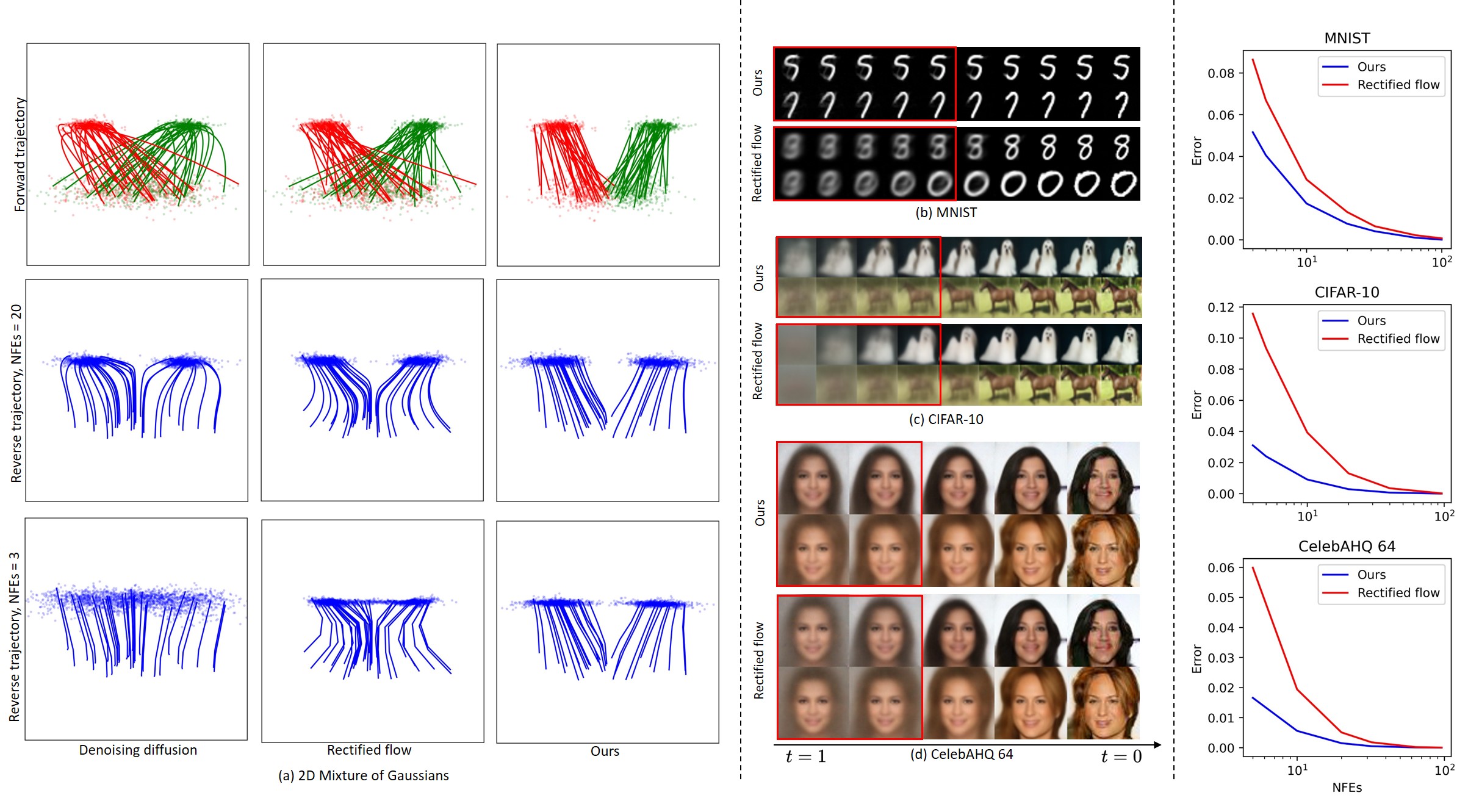
Figure 1: Forward and reverse trajectories of denoising diffusion model (Ho et al., 2020), rectified flow (Liu et al., 2022), and our method on 2D dataset (left). The intersection between forward trajectories makes reverse trajectories collapse toward the average direction, resulting in increased curvature and suboptimal sample qualities with a limited number of function evaluations (NFE). In contrast, our approach successfully unties the crossover between forward trajectories, leading to low-curvature reverse trajectories. This phenomenon also holds true in high-dimensional spaces, as demonstrated by reverse process visualization on MNIST, CIFAR-10, and CelebAHQ (64 $\times$ 64) datasets (middle). As a result, our method makes less truncation error when the number of function evaluations (NFE) is small (right).

However, drawing samples from ODE-based generative models requires multiple evaluations of a neural network for accurate numerical simulation, leading to slow sampling speed. While many studies have attempted to develop fast samplers for pre-trained models (Lu et al., 2022; Zhang & Chen, 2022), there seems to be a limit to lowering the costs. We attribute the reason to the high curvature of the learned generative trajectories. The curvature is intriguing since it is directly related to the truncation error of a numerical solver. Intuitively, zero curvature means that generative ODEs can be accurately solved with only one function evaluation. Since a generative process is a time reversal of the forward process, it is evident that its curvature is also somehow determined by the forward process, but the exact mechanism is yet unexplored. We find that the rectified flow perspective offers an interesting insight into the relationship between the forward process and the curvature. Based on our observation, we propose an efficient method of training the forward process to reduce curvature. Specifically, our contributions are as follows:

• We investigate the relationship between the forward process and curvature from a rectified flow perspective. We find that the degree of intersection between forward trajectories is positively related to the curvature of generative processes.

• We propose an efficient method of learning the forward process to reduce the degree of intersection between forward trajectories without any ODE/SDE simulation. We show that our method can be seen as a $\beta$-VAE (Higgins et al., 2016) with a time-conditional decoder.

• Experiments show that our method achieves lower curvature than previous models and, therefore, demonstrates decreased sampling costs while maintaining competitive performance.

2 Background

ODE/SDE-based generative models effectively model complex distributions by repeatedly composing a neural network, making trade-offs between execution time and sample quality. In this paper, we focus on ODE-based generative models since they yield the same marginal distribution as SDEs while being conceptually simpler and faster to sample (Song et al., 2020).

Different from continuous normalizing flows (CNF) (Chen et al., 2018), recent ODE-based models do not require ODE simulations during training and therefore are more scalable. At a high level, they define a forward coupling $q(\boldsymbol{x},\boldsymbol{z})$ between data distribution $p(\boldsymbol{x})$ and prior distribution $p(\boldsymbol{z})$ and subsequently an interpolation $\boldsymbol{x}_{t}(\boldsymbol{x},\boldsymbol{z})$ for $t\in[0,1]$ between a pair $(\boldsymbol{x},\boldsymbol{z})\sim q(\boldsymbol{x},\boldsymbol{z})$ such that $\boldsymbol{x}_{0}(\boldsymbol{x},\boldsymbol{z})=\boldsymbol{x}$ and $\boldsymbol{x}_{1}(\boldsymbol{x},\boldsymbol{z})=\boldsymbol{z}$. Training objectives are variants of the denoising autoencoder objective

$$\min_{\boldsymbol{\theta}}\mathbb{E}_{t\sim U(0,1)}\mathbb{E}_{\boldsymbol{x},\boldsymbol{z}\sim q(\boldsymbol{x},\boldsymbol{z})}[\lambda(t)||\boldsymbol{x}-\boldsymbol{x}_{\theta}(\boldsymbol{x}_{t}(\boldsymbol{x},\boldsymbol{z}),t)||_{2}^{2}],$$ (1)

where $\lambda(t)$ is a weighting function. Here, a neural network $\boldsymbol{x}_{\theta}(\boldsymbol{x}_{t},t)$ is trained to reconstruct the data $\boldsymbol{x}$ from the corrupted observation $\boldsymbol{x}_{t}$. In the following, we briefly review two popular instances of such models: the denoising diffusion model and rectified flow. We refer the readers to Appendix A for a detailed background.

Denoising diffusion models

Denoising diffusion models (Ho et al., 2020) employ the prior $p(\boldsymbol{z})=\mathcal{N}(\mathbf{0},\boldsymbol{I})$, forward coupling $q(\boldsymbol{x},\boldsymbol{z})=p(\boldsymbol{x})p(\boldsymbol{z})$, and a nonlinear interpolation

$$\boldsymbol{x}_{t}(\boldsymbol{x},\boldsymbol{z})=\alpha(t)\boldsymbol{x}+\sqrt{1-\alpha(t)^{2}}\boldsymbol{z}$$ (2)

with a predefined nonlinear function $\alpha(t)$. $\lambda(t)$ is often adjusted to improve the perceptual quality for image synthesis (Ho et al., 2020). Sampling can be done by solving probability flow ODEs (Song et al., 2020).

Rectified flows

However, the choice of Eq. (2) seems unnatural from a rectified flow perspective as it unnecessarily increases the curvature of generative trajectories. In rectified flow (Liu et al., 2022; Liu, 2022), the intermediate sample $\boldsymbol{x}_{t}$ is rather defined as a linear interpolation

$$\boldsymbol{x}_{t}(\boldsymbol{x},\boldsymbol{z})=(1-t)\boldsymbol{x}+t\boldsymbol{z}$$ (3)

since it has a constant velocity across $t$ for given $\boldsymbol{x}$ and $\boldsymbol{z}$. After training, sampling is done by solving the following ODE backward:

$$d\boldsymbol{z}_{t}=\frac{\boldsymbol{z}_{t}-\boldsymbol{x}_{\theta}(\boldsymbol{z}_{t},t)}{t}dt,$$ (4)

where $dt$ is an infinitesimal timestep. In the optima, Eq. (4) maps $\boldsymbol{z}_{1}$ from $p(\boldsymbol{z})$ to $\boldsymbol{z}_{0}$ following $p(\boldsymbol{x})$. Instead of predicting $\boldsymbol{x}$, Liu et al. (2022) directly learns the velocity ${\boldsymbol{v}}_{\theta}(\boldsymbol{z}_{t},t)=\frac{\boldsymbol{z}_{t}-\boldsymbol{x}_{\theta}(\boldsymbol{z}_{t},t)}{t}$. The effectiveness of this sampler in reducing the sampling costs has been previously investigated in Karras et al. (2022) under the variance-exploding context. Also, Eqs. (3) and (4) are a special case of flow matching (Lipman et al., 2022). See Appendix A.2. We build our method based on this framework, using the linear interpolation and the ODE in Eq. (4) for sampling.

3 Curvature Minimization

3.1 Curvature

For a generative process $\boldsymbol{Z}=\{\boldsymbol{z}_{t}(\boldsymbol{z})\}$ with the initial value $\boldsymbol{z}_{1}(\boldsymbol{z})=\boldsymbol{z}$ , we informally define curvature as the extent to which the trajectory deviates from a straight path:

$$C(\boldsymbol{Z})=\mathbb{E}_{t}\left\|\boldsymbol{z}_{1}(\boldsymbol{z})-\boldsymbol{z}_{0}(\boldsymbol{z})-\frac{\partial}{\partial t}\boldsymbol{z}_{t}(\boldsymbol{z})\right\|_{2}^{2},$$ (5)

which is equal to the straightness used in Liu et al. (2022). The average curvature $\mathbb{E}_{\boldsymbol{z}\sim p(\boldsymbol{z})}[C(\boldsymbol{Z})]$ should be the main concern in designing the ODE-based models since it is directly related to the truncation error of numerical solvers. Zero curvature means the path is completely straight. Therefore, a single step of the Euler solver is sufficient to obtain an accurate solution.

Since a generative process is a time reversal of the forward process, its curvature is determined by the forward process. As an illustrative example, consider a generative ODE that is trained on Eq. (1). In the optima, $\boldsymbol{x}_{{\boldsymbol{\theta}}}(\boldsymbol{z}_{t},t)$ is a minimum mean squared error estimator $\mathbb{E}[\boldsymbol{x}|\boldsymbol{x}_{t}=\boldsymbol{z}_{t}]$, and the average curvature of the generative processes governed by Eq.(4) becomes

$$\mathbb{E}_{\boldsymbol{z},t}\left\|\boldsymbol{z}_{1}(\boldsymbol{z})-\boldsymbol{z}_{0}(\boldsymbol{z})-\frac{1}{t}\boldsymbol{z}_{t}(\boldsymbol{z})+\frac{1}{t}\mathbb{E}[\boldsymbol{x}|\boldsymbol{x}_{t}=\boldsymbol{z}_{t}(\boldsymbol{z})]\right\|_{2}^{2},$$ (6)

which is a function of the posterior $q(\boldsymbol{x}|\boldsymbol{x}_{t})$. Since we define $\boldsymbol{x}_{t}$ as an interpolation between $\boldsymbol{x}$ and $\boldsymbol{z}$, the posterior is determined by the forward coupling $q(\boldsymbol{x},\boldsymbol{z})$. In previous work, $q(\boldsymbol{x},\boldsymbol{z})$ is fixed, and so is the curvature of the generative process in optima. In the following, we further examine the relationship between forward coupling and curvature and show that we can improve the curvature by finding better $q(\boldsymbol{x},\boldsymbol{z})$.

3.2 Curvature and the degree of intersection

Specifically, we observe that Eq. (6) is related to the degree of intersection of the forward trajectories

$$I(q)=\mathbb{E}_{t,\boldsymbol{x},\boldsymbol{z}\sim q(\boldsymbol{x},\boldsymbol{z})}[||\boldsymbol{z}-\boldsymbol{x}-\mathbb{E}[\boldsymbol{z}-\boldsymbol{x}|\boldsymbol{x}_{t}(\boldsymbol{x},\boldsymbol{z})]||_{2}^{2}],$$ (7)

which becomes zero when there is no intersection at any $\boldsymbol{x}_{t}$. As shown in Fig. 1, the intersection between forward trajectories makes the reverse vector field collapse toward the average direction, leading to high curvature. As the degree of intersection decreases, the reverse paths are gradually straightened. When $I(q)=0$, the posterior $q(\boldsymbol{x}|\boldsymbol{x}_{t})$ becomes a Dirac delta function, $\mathbb{E}[\boldsymbol{x}|\boldsymbol{x}_{t}=\boldsymbol{z}_{t}(\boldsymbol{z})]=\boldsymbol{z}_{0}(\boldsymbol{z})$ for every $t$, and Eq. (6) becomes zero, i.e., the paths are completely straight. Therefore, it is natural to seek a forward coupling $q(\boldsymbol{x},\boldsymbol{z})$ that minimizes Eq. (7). We can estimate Eq. (7) by minimizing the following upper bound with respect to ${\boldsymbol{\theta}}$.

Proposition 1.

Let $\boldsymbol{x}_{t}(\boldsymbol{x},\boldsymbol{z})$ be the linear interpolation defined as Eq. (3). Then, we have

$$I(q)\leq\mathbb{E}_{t,\boldsymbol{x},\boldsymbol{z}\sim q(\boldsymbol{x},\boldsymbol{z})}\left[\frac{1}{t^{2}}||\boldsymbol{x}-\boldsymbol{x}_{\boldsymbol{\theta}}(\boldsymbol{x}_{t},t)||_{2}^{2}\right].$$ (8)

The bound is tight when $\boldsymbol{x}_{\boldsymbol{\theta}}(\boldsymbol{x}_{t},t)=\mathbb{E}[\boldsymbol{x}|\boldsymbol{x}_{t}]$.

Sketch of Proof.

Using Eq. (3), we obtain $\boldsymbol{z}-\boldsymbol{x}=(\boldsymbol{x}_{t}-\boldsymbol{x})/t$. Plugging it into Eq. (7), we have

$$I(q)=\mathbb{E}_{t,\boldsymbol{x},\boldsymbol{z}\sim q(\boldsymbol{x},\boldsymbol{z})}[||\frac{1}{t}(\boldsymbol{x}-\mathbb{E}[\boldsymbol{x}|\boldsymbol{x}_{t}])||_{2}^{2}],$$ (9)

which is bounded by Eq. (8). ∎

For the independent coupling $q(\boldsymbol{x},\boldsymbol{z})=p(\boldsymbol{x})p(\boldsymbol{z})$, the upper bound of $I(q)$ coincides with Eq. (1) with $\lambda(t)=1/t^{2}$, which is the training loss of Liu et al. (2022). In this sense, Liu et al. (2022) estimates the upper bound of the degree of intersection of the independent coupling but does not really minimize it. Intuitively, the degree of intersection can be measured by the reconstruction error of an optimal decoder since the decoding is more difficult when multiple inputs are encoded into a single point. See Fig. 2 for an illustration.

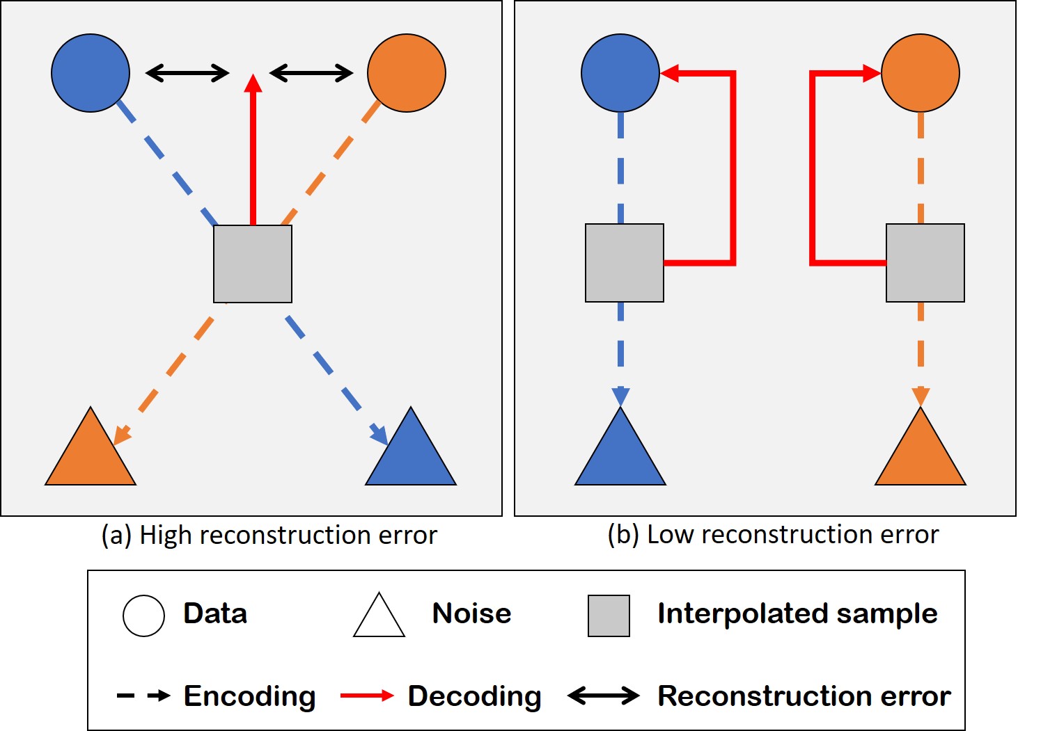
Figure 2: Reconstruction error is (a) high when forward trajectories intersect (b) and low when they do not.

3.3 Parameterizing $q(\boldsymbol{x},\boldsymbol{z})$

After estimating $I(q)$ by updating ${\boldsymbol{\theta}}$, we search for $q$ that minimizes $I(q)$. Although there are many ways to solve this optimization problem, there are two practical considerations. First, the optimization needs to be efficient. Moreover, $q(\boldsymbol{z}|\boldsymbol{x})$ should define a smooth map from $\boldsymbol{x}$ to $\boldsymbol{z}$ since we have to approximate $\mathbb{E}[\boldsymbol{x}|\boldsymbol{x}_{t}]$ using a neural network with finite capacity in practice. Therefore, we propose to parameterize the coupling as a neural network $q_{\boldsymbol{\phi}}(\boldsymbol{x},\boldsymbol{z})=q_{\boldsymbol{\phi}}(\boldsymbol{z}|\boldsymbol{x})p(\boldsymbol{x})$, where we define $q_{\boldsymbol{\phi}}(\boldsymbol{z}|\boldsymbol{x})$ as a Gaussian distribution. With $q_{\boldsymbol{\phi}}(\boldsymbol{z})=\int q_{\boldsymbol{\phi}}(\boldsymbol{x},\boldsymbol{z})d\boldsymbol{x}$ and a weight $\beta$, we optimize

$$\min_{\boldsymbol{\phi}}I(q_{\boldsymbol{\phi}})+\beta D_{KL}(q_{\boldsymbol{\phi}}(\boldsymbol{z})||p(\boldsymbol{z})).$$ (10)

The second KL term ensures $q_{\boldsymbol{\phi}}(\boldsymbol{x},\boldsymbol{z})$ is a valid coupling between $p(\boldsymbol{x})$ and $p(\boldsymbol{z})$. See Appendix B for more details.

Joint training

In practice, we jointly minimize Eqs. (8) and (10) with respect to both $\theta$ and $\phi$. This leads to our loss function

$$\min_{{\boldsymbol{\theta}},{\boldsymbol{\phi}}}\ \mathbb{E}_{t,\boldsymbol{x},\boldsymbol{z}\sim q_{\boldsymbol{\phi}}(\boldsymbol{x},\boldsymbol{z})}[\frac{1}{t^{2}}||\boldsymbol{x}-\boldsymbol{x}_{\boldsymbol{\theta}}(\boldsymbol{x}_{t}(\boldsymbol{x},\boldsymbol{z}),t)||_{2}^{2}$$

$$+\beta D_{KL}(q_{\boldsymbol{\phi}}(\boldsymbol{z}|\boldsymbol{x})||p(\boldsymbol{z}))],$$ (11)

which resembles the $\beta$-VAE objective (Higgins et al., 2016) in that Eq. (11) reduces to the $\beta$-VAE loss if we fix $t$ to $1$. Since the decoder $\boldsymbol{x}_{\theta}$ is conditioned on time step, ODE-based models can synthesize higher quality samples than $\beta$-VAEs by iteratively refining the blurry initial predictions. From this viewpoint, previous methods (Liu et al., 2022; Ho et al., 2020) can be seen as degenerate cases where the encoder $q_{\boldsymbol{\phi}}(\boldsymbol{z}|\boldsymbol{x})$ collapses into the prior by setting $\beta\rightarrow\infty$. See Fig. 3 for a visual schematic of our method.

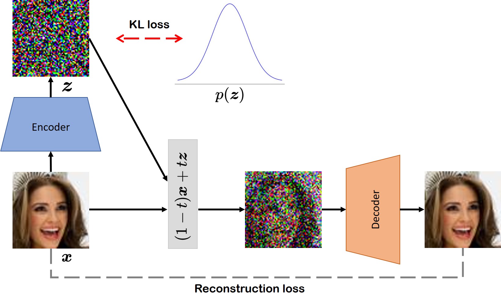
Figure 3: A visual schematic of the proposed method.

4 Related Works

Alternative forward processes

There have been several approaches to finding alternative forward processes for diffusion models. It has been demonstrated that other types of degradation, such as blurring, masking, or pre-trained neural encoding, can be used for the forward process (Rissanen et al., 2022; Lee et al., 2022; Hoogeboom & Salimans, 2022; Daras et al., 2022; Gu et al., 2022; Bansal et al., 2022). However, they are either purely heuristic or rely on an inductive bias that is not necessarily well-supported by theory.

Learning forward process

A few studies attempted to learn the forward process. Kingma et al. (2021) proposed to learn the signal-to-ratio function of the forward process jointly with generative components. However, the inference model of Kingma et al. (2021) is linear and thus has limited expressivity. Zhang & Chen (2021) proposed nonlinear diffusion models, where the drift function of the forward SDEs are neural networks. Although they introduce more flexibility in inference models, training requires the simulation of forward/reverse SDEs, which causes a significant computational overhead. Our method possesses the advantages of both methods. Our inference model is expressive since we set $q(\boldsymbol{z}|\boldsymbol{x})$ as a neural network. Since we define $\boldsymbol{x}_{t}$ as an interpolation between $\boldsymbol{x}$ and $\boldsymbol{z}$ and $q_{\phi}(\boldsymbol{x}_{t}|\boldsymbol{x})$ as a Gaussian distribution, sampling is done with one forward pass for an arbitrary $t$, enabling efficient training as in previous methods (Ho et al., 2020; Liu et al., 2022). Moreover, even though the nonlinear forward process appeared to improve the sampling efficiency of diffusion models (Zhang & Chen, 2021), the exact mechanism of the improved sampling speed was vague. In this paper, we convey a clear motivation for learning the forward process by revealing the relationship between the forward process and the curvature of the generative trajectories.

Fast samplers

Accelerating the sampling speed of diffusion models is an active research topic, which is often tackled by developing fast solvers (Lu et al., 2022; Zhang & Chen, 2022). Our work is in an orthogonal direction since they focus on taming the high curvature ODEs while we aim to minimize the curvature itself. We expect the effect of these methods to be additive to ours and leave the detailed investigation for future work.

Straightness of Neural ODEs

The importance of the straightness of neural ODEs in reducing the sampling cost has been previously discussed. Based on Benamou-Brenier formulation of the optimal transport problem (Benamou & Brenier, 2000), Finlay et al. (2020) regularized the norm of the vector field of the CNFs to encourage the straightness, which is later generalized in Kelly et al. (2020) where the norm of the $K$-th order derivative is minimized. Since CNFs are trained on the maximum likelihood objective, any vector field that defines the transport map from $p(\boldsymbol{z})$ to $p(\boldsymbol{x})$ is optimal, and it is therefore possible to narrow down the search space by utilizing the additional constraint without drastically compromising the performance. In contrast, recent ODE-based generative models (Song & Ermon, 2019; Ho et al., 2020; Liu et al., 2022) train the neural ODE to match a pre-defined forward flow using Eq. (1). Thus the solution is unique, and any additional regularization makes models deviate from optima.

Optimizing coupling

Concurrent with our work, Pooladian et al. (2023) proposed to optimize $q(\boldsymbol{x},\boldsymbol{z})$ and showed several desirable properties such as improved sampling efficiency and reduced gradient variance during training. While we parameterize $q(\boldsymbol{x},\boldsymbol{z})$ as a neural network, they construct a doubly-stochastic matrix for $q(\boldsymbol{x},\boldsymbol{z})$ and apply computational methods to find the optimal coupling between two empirical distributions. In practice, the optimization is done either with heuristics or using mini-batch samples every iteration due to the computational burden. They showed that in an ideal case with infinite batch size, 1) $I(q)$ goes to zero, 2) $C({\mathbf{Z}})$ becomes zero, and 3) the resulting generative model becomes an optimal transport plan. Although minimizing transportation costs has impacts beyond the context of generative modeling, we focus on accelerating the sampling of ODE-based generative models in this paper, so we design our method to achieve straight generative paths regardless of transportation costs.

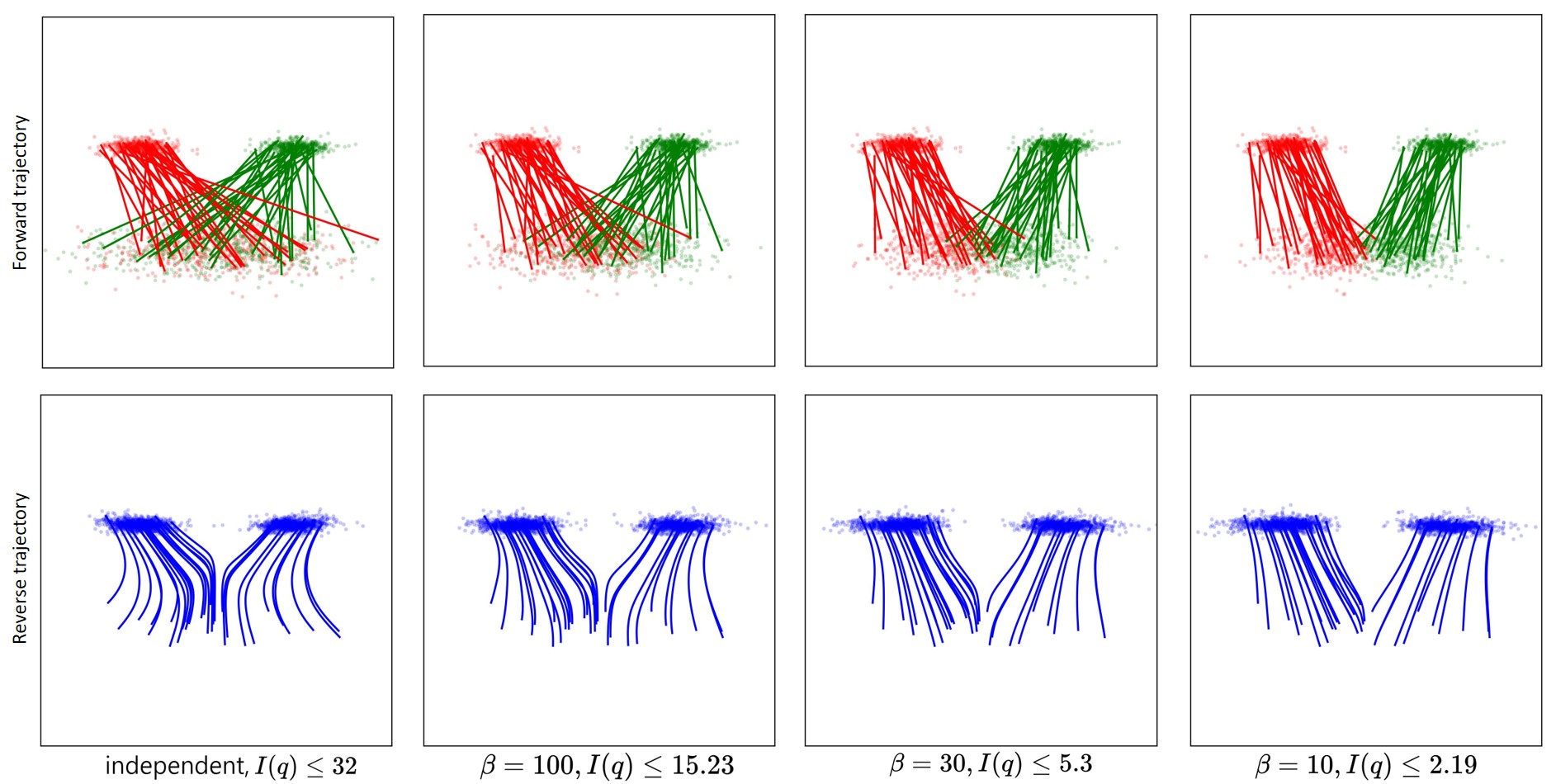
Figure 4: The relationship between the degree of intersection between forward trajectories and curvature of reverse trajectories. The first column shows forward and reverse trajectories induced by the independent coupling $q(\boldsymbol{x},\boldsymbol{z})=p(\boldsymbol{x})p(\boldsymbol{z})$. As the degree of intersection between forward trajectories is decreased by lowering $\beta$, reverse paths are gradually straightened.

5 Experiment

5.1 2D dataset

Fig. 4 demonstrates the visual results and the estimated upper bounds of the degree of intersection on the 2D toy dataset. The leftmost column shows the forward trajectories induced by the independent coupling $q(\boldsymbol{x},\boldsymbol{z})=p(\boldsymbol{x})p(\boldsymbol{z})$ used in previous work. Since a data point can be mapped to any noise, the forward trajectories largely intersect with each other, and as a result, the reverse trajectories collapse toward the average direction where the actual density is low, and the curvature increases as the reverse trajectories need to bend toward the modes. As $\beta$ decreases, $q_{\phi}(\boldsymbol{z}|\boldsymbol{x})$ tries to untie the tangled trajectories, leading to low curvature.

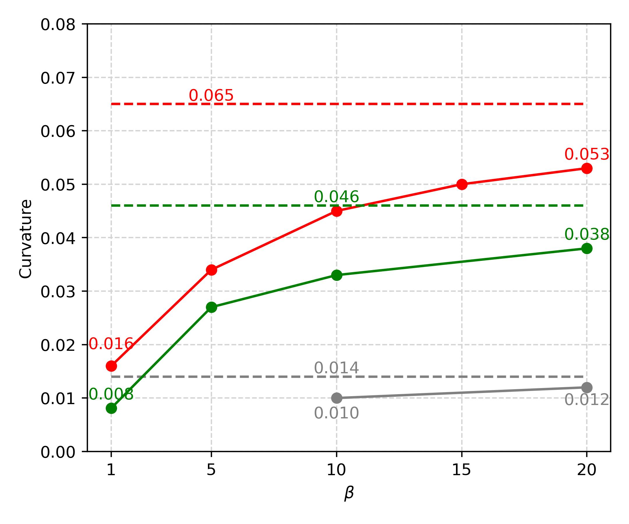
Figure 5: Effects of $\beta$ on curvature. The results on MNIST, CIFAR-10, and CelebAHQ ($64\times 64$) are indicated by red, green, and gray colors. Dashed lines indicate the curvatures of the independent coupling baselines.

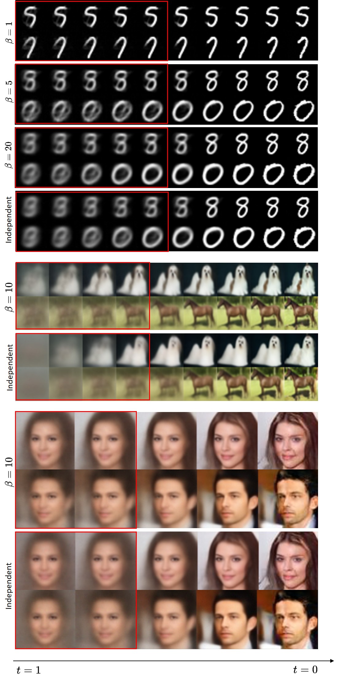
Figure 6: Visualization of intermediate samples $\boldsymbol{x}_{\boldsymbol{\theta}}(\boldsymbol{z}_{t},t)$ with varying $\beta$. Lower $\beta$ allows for sharper initial predictions, as indicated by red boxes.

5.2 Image generation

We further conduct an experiment on the image dataset to investigate the relationship between $I(q)$ and $\mathbb{E}[C(\boldsymbol{Z})]$ in the high-dimensional space. We estimate $\mathbb{E}[C(\boldsymbol{Z})]$ by simulating $10,000$ generative trajectories using the Euler solver with 128 steps and then divide by the number of pixels. As shown in Fig. 5, the average curvature is the highest when using independent forward coupling $q(\boldsymbol{x},\boldsymbol{z})=p(\boldsymbol{x})p(\boldsymbol{z})$ and lowered as $\beta$ decreases. Fig. 6 shows that the generative vector field induced by independent coupling $q(\boldsymbol{x},\boldsymbol{z})=p(\boldsymbol{x},\boldsymbol{z})$ initially predicts the blurry images and then bends toward the mode, resulting in the high curvature. Lower $\beta$ yields more consistent results across the time steps.

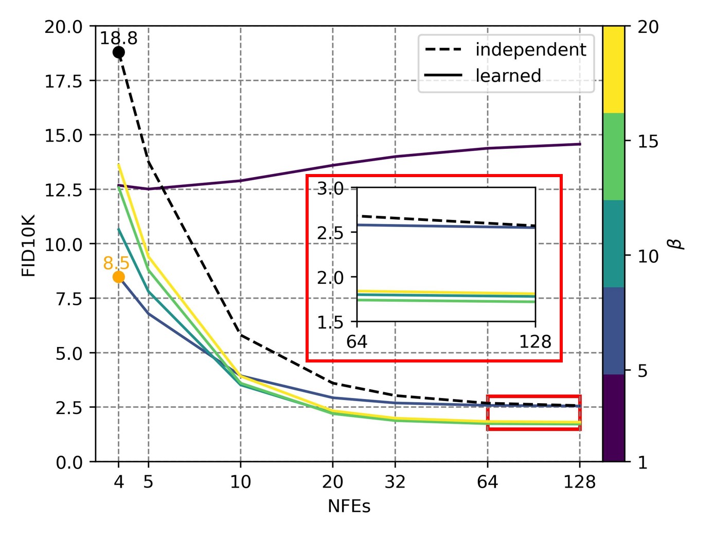
(a) Quantitative results

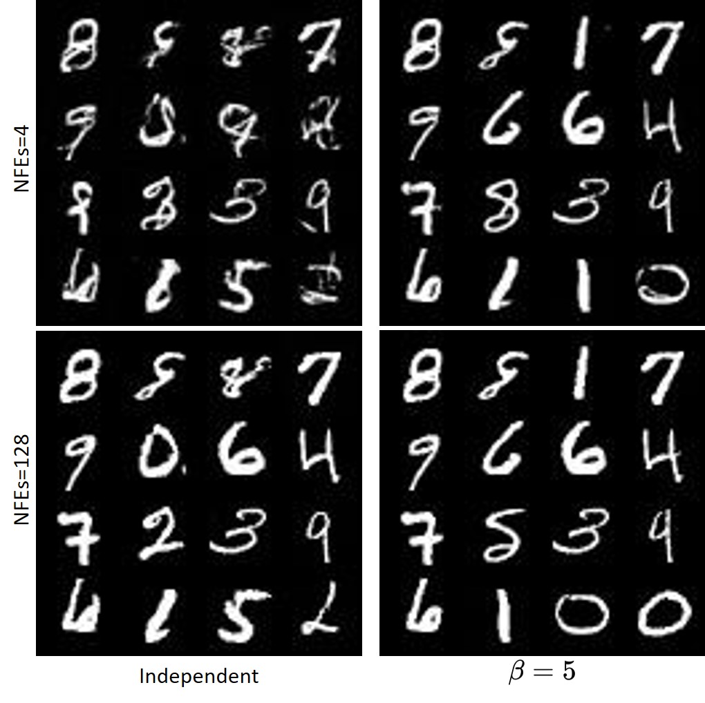
(b) Qualitative results

Figure 7: Trade-off between FID10K and the number of function evaluations (NFE) with varying $\beta$. The low curvature generative process produces more high-quality samples than the baseline with limited NFEs.

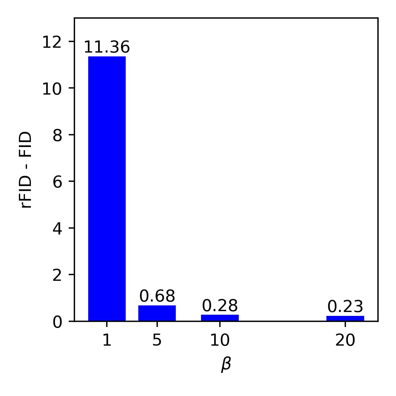
(a) FID gap with respect to $\beta$

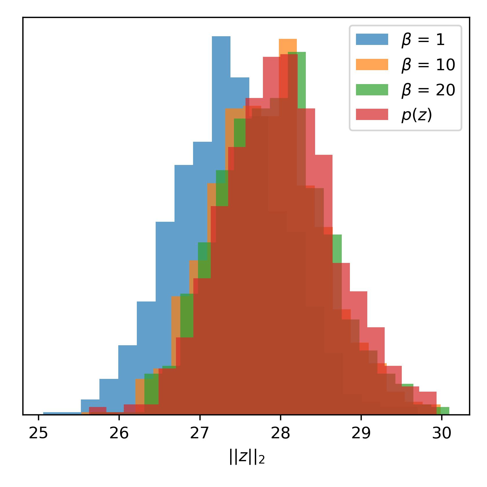
(b) Distribution of $||\boldsymbol{z}||_{2}$

Figure 8: The gap between reconstruction FID (rFID) and FID values (a), and distribution of the norm of $\boldsymbol{z}\sim q_{\boldsymbol{\phi}}(\boldsymbol{z})$ (b). rFID is measured using samples reconstructed from $q_{\boldsymbol{\phi}}(\boldsymbol{z})$.

Fig. 7 shows that the model trained with the lower $\beta$ performs better with the limited NFEs and asymptotically approaches the performance of baseline indicated by a dashed line. When $\beta$ is as low as $1$, the generative process is almost straight, but the sample quality is degraded because of high $D_{KL}(q_{\phi}(\boldsymbol{z})||p(\boldsymbol{z}))$ (i.e. the prior hole problem). As shown in Fig. 8, the gap between reconstruction FID (rFID) and FID is large when $\beta=1$ and gradually becomes smaller as $\beta$ increases. Moreover, the distribution of the norm of latent vectors gradually approaches $p(\boldsymbol{z})$ as $\beta$ increases. From this observation, we can see that $\beta$ is an important hyperparameter that determines the trade-off between sample quality and computational cost. We find that there are little advantages of setting $\beta$ to $\infty$ as in previous work (Liu et al., 2022; Ho et al., 2020). It is an overkill for reducing the prior hole and leads to poor sampling efficiency.

In Fig. 9 and Tab. 1, we provide additional qualitative and quantitative comparisons between our method and rectified flow baseline on FFHQ 64 $\times$ 64, AFHQ 64 $\times$ 64, and CelebAHQ 256 $\times$ 256 datasets, which further confirm the validity of our method.

Setting \ NFEs	4	5	10	20	32	64	128
$\beta=10$	32.58	25.33	13.21	8.85	7.54	6.91	7.01
$\beta=20$	38.23	29.12	14.03	8.78	7.08	5.95	5.72
$\beta=30$	41.16	30.75	14.37	8.76	6.90	5.45	4.93
Independent	55.90	40.96	17.29	9.79	7.55	5.89	5.26

(a) FFHQ 64 $\times$ 64

Setting \ NFEs	4	5	10	20	32	64	128
$\beta=10$	21.80	18.04	11.80	9.05	8.22	7.47	7.21
$\beta=20$	25.73	20.11	10.56	6.89	5.74	4.92	4.55
$\beta=30$	30.84	23.08	11.17	6.66	5.37	4.40	3.96
Independent	54.10	42.64	18.53	8.60	6.19	4.85	4.36

(b) AFHQ 64 $\times$ 64

Setting \ NFEs	4	5	10	20	32	64	128
$\beta=10$	58.30	51.02	33.53	22.91	19.49	17.57	16.94
$\beta=40$	62.21	52.92	31.70	18.70	14.03	11.39	10.37
Independent	100.39	84.50	48.95	26.42	18.45	12.78	10.38

(c) CelebAHQ 256 $\times$ 256

Table 1: FID10K comparison on three image datasets.

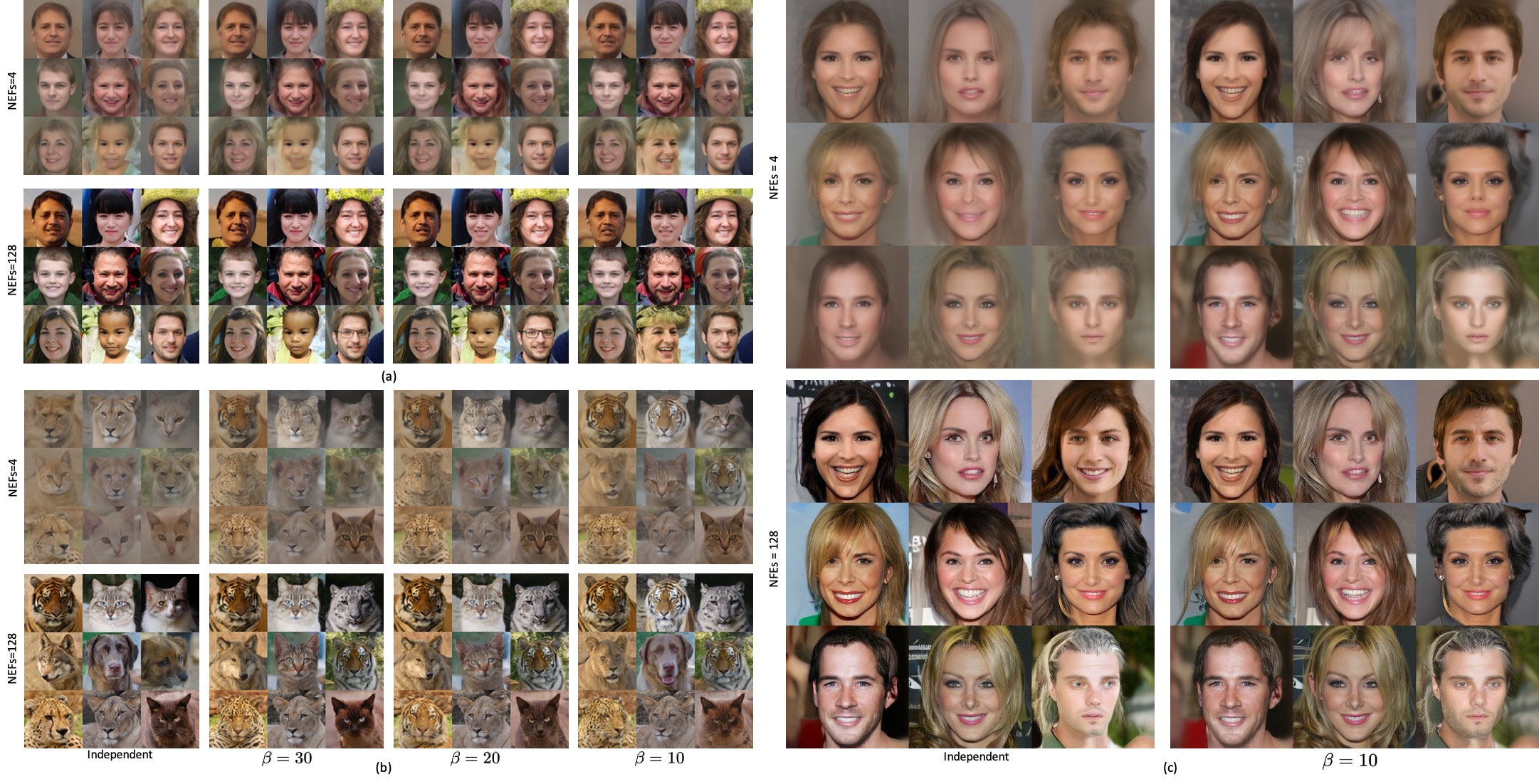
Figure 9: Qualitative comparison between our method and baseline on FFHQ 64 $\times$ 64 (a), AFHQ 64 $\times$ 64 (b), and CelebAHQ 256 $\times$ 256 (c) datasets.

5.3 Distillation

Even though distillation is an effective way to train the one-step student models from the teacher diffusion models, the performance of the student model is suboptimal due to the distillation error (Liu et al., 2022; Luhman & Luhman, 2021; Salimans & Ho, 2022). Given that the teacher trajectories with higher NFEs are more difficult to distill, our low-curvature generative ODEs would make less distillation error since they achieve the same level of sample quality using relatively lower NFEs. Based on this intuition, we investigate the effect of our method on reducing the distillation error. As shown in Table 2, the teacher ODE with $\beta=10$ achieves a similar FID score using half as many NFEs compared to the baseline model. This resulted in a smaller distillation error and an improved FID score of the one-step model while reducing the cost of generating paired data by half. Fig. 10 demonstrates that our method with $\beta=10$ obtains a superior one-step model than baseline with independent coupling in terms of sample fidelity.

Table 2: Effects of curvature on distillation performance. The results of independent coupling and our method with $\beta=10$ are reported. Distillation error is measured as a mean-squared error on the test set.

	Independent		$\beta=10$
	FID / Error	NFEs	FID / Error	NFEs
Teacher	3.60 / -	20	3.52 / -	10
Distilled	6.25 / 0.0208	1	4.41 / 0.0157	1

(a) $\beta=10$

(b) Independent

Figure 10: Synthesis results of one-step models.

5.4 Size of encoder

Since we train $q_{\boldsymbol{\phi}}(\boldsymbol{z}|\boldsymbol{x})$, a natural question is how much additional computational cost is needed for training our model. We experiment with two settings of the encoder, same and small. In same setting, we use the identical architecture with a generative component except that the number of output channels is twice for predicting a diagonal covariance. In small setting, we use roughly 20 times smaller architecture for the encoder model. See Appendix C for a detailed configuration. As shown in Table 3, a small encoder performs just as well or even better than a larger encoder, and part of the reason is that we can use a larger batch size in the small setting. The additional cost of our method is negligible with the use of a lightweight architecture for $q_{\boldsymbol{\phi}}(\boldsymbol{z}|\boldsymbol{x})$, so we stick to small setting throughout our experiments.

Table 3: Performance comparison of same and small encoder settings on CIFAR-10 dataset, measured by FID10K.

Setting \ NFEs	128	40	20	10	5	4
Same Encoder	5.52	6.23	7.74	11.49	22.90	30.97
Small Encoder	5.39	6.07	7.51	11.19	22.33	30.16

Table 4: Comparison with state-of-the-arts on CIFAR-10 dataset. * Our reimplementation.

Method	NFEs($\downarrow$)	IS ($\uparrow$)	FID ($\downarrow$)	Recall ($\uparrow$)
GANs
StyleGAN2 (Karras et al., 2020a)	1	9.18	8.32	0.41
StyleGAN2 + ADA (Karras et al., 2020a)	1	9.40	2.92	0.49
StyleGAN2 + DiffAug (Zhao et al., 2020)	1	9.40	5.79	0.42
ODE/SDE-based models
Denoising Diffusion GAN (T=1) (Xiao et al., 2021)	1	8.93	14.6	0.19
DDPM (Ho et al., 2020)	1000	9.46	3.21	0.57
NCSN++ (VE SDE) (Song et al., 2020)	2000	9.83	2.38	0.59
LSGM (Vahdat et al., 2021)	138	-	2.10	-
DFNO (Zheng et al., 2022)	1	-	5.92	-
Knowledge distillation (Luhman & Luhman, 2021)	1	8.36	9.36	0.51
Progressive distillation (Salimans & Ho, 2022)	1	-	9.12	-
Rectified Flow (RK45) (Liu et al., 2022)	127	9.60	2.58	0.57
2-Rectified Flow (RK45)	110	9.24	3.36	0.54
3-Rectified Flow (RK45)	104	9.01	3.96	0.53
2-Rectified Flow Distillation	1	9.01	4.85	0.50
Our results
Rectified Flow* (config A, RK45)	134	9.18	2.87	-
Rectified Flow* (config B, RK45)	132	9.48	2.66	0.62
Rectified Flow* (config B, Heun’s $2^{\text{nd}}$ order method)	9	8.48	12.92	-
Rectified Flow* (config B, Heun’s $2^{\text{nd}}$ order method)	5	7.04	37.19	-
Ours ($\beta=20$, config B, RK45)	118	9.55	2.45	0.64
Ours ($\beta=20$, config B, Heun’s $2^{\text{nd}}$ order method)	9	8.75	9.96	-
Ours ($\beta=20$, config B, Heun’s $2^{\text{nd}}$ order method)	5	7.83	24.40	-
Ours ($\beta=10$, config A, RK45)	110	9.32	3.37	0.61
Ours ($\beta=10$, config A, Heun’s $2^{\text{nd}}$ order method)	9	8.67	8.66	-
Ours ($\beta=10$, config A, Heun’s $2^{\text{nd}}$ order method)	5	8.09	18.74	-

5.5 Comparison with state-of-the-arts

Table 4 shows the unconditional synthesis results of our approach on the CIFAR-10 dataset. Results of recent methods are also provided as a reference. We experiment with two configurations, config A and config B, which we detail in Appendix C. We try three solvers, Euler solver, Heun’s $2^{\text{nd}}$ order method, and the black-box RK45 method from Scipy (Virtanen et al., 2020), and find that RK45 works well when we are able to fully simulate ODEs while Heun’s $2^{\text{nd}}$ order method performs better than other solvers with small NFEs. As shown in the table, we can see that the performance gap between our method and the baseline is huge when the sampling budget is limited. For instance, our method with $\beta=10$ achieved an FID score of 18.74, which is significantly better than the baseline’s score of 37.19 when NFEs is 5. Surprisingly, our method with $\beta=20$ exhibits superior sample qualities across all NFEs, even in the case of full sampling using the RK45 solver. See Fig. 11 for visual comparison. Additional qualitative results are provided in Appendix D.

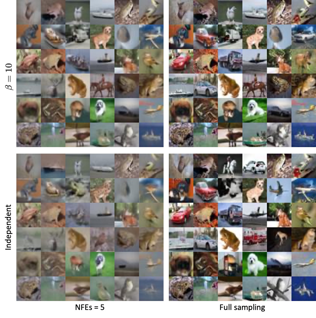
Figure 11: Qualitative comparison between our method ($\beta=10$) and baseline on CIFAR-10.

6 Discussion and Limitations

One limitation of our method is that for our encoding distribution $q_{\boldsymbol{\phi}}(\boldsymbol{z}|\boldsymbol{x})$, we use a Gaussian distribution for theoretical and practical conveniences: sampling is easily implemented in a differentiable manner, and KL divergence is tractable. However, our simple Gaussian encoder cannot eliminate the intersection completely. We believe that it would be beneficial to use a more flexible encoding distribution, for instance, using the hierarchical latent variable as in Child (2020); Vahdat & Kautz (2020).

Additionally, the trade-off between sample quality and computational cost is determined by the value of $\beta$, which must be manually selected by a practitioner. In Sec. 5.2, we observe that too small $\beta$ value causes the prior hole problem. This is problematic as one has to train a model from scratch for each value of $\beta$, which would potentially lead to excessive energy consumption. However, using a reasonably high value of $\beta$ consistently outperforms the baseline regardless of the sampling budget, as shown in our experiments. Therefore, one could reduce the sampling cost without compromising performance by conservatively setting $\beta$ to a high value in most cases.

7 Conclusion

In this paper, we mainly discussed the curvature of the ODE-based generative models, which is crucial for sampling efficiency. We revealed the relationship between the degree of intersection between forward trajectories and the curvature and presented an efficient algorithm to reduce the intersection by training a forward coupling. We demonstrated that our method successfully reduces the trajectory curvature, thereby enabling accurate ODE simulation with significantly less sampling budget. Furthermore, we showed our method effectively decreases the distillation error, improving the performance of one-step student models. Our approach is unique and complementary to other acceleration methods, and we believe it can be used in conjunction with other techniques to further decrease the sampling cost of ODE-based generative models.

8 Societal Impacts.

We anticipate this work will have positive effects, as our method reduces the computational costs required during the sampling of ODE-based generative models. However, the same technology can also be used to create malicious content, and thus, proper regulations need to be put in place to ensure that this technology is used responsibly and ethically.

Appendix A Preliminaries

A.1 Rectified flows

Diffusion models have been interpreted as the variational approaches (Sohl-Dickstein et al., 2015; Ho et al., 2020) or score-based models (Song & Ermon, 2019; Song et al., 2020), and their deterministic samplers are derived post hoc. However, stochasticity is not a key factor in the success of these models. The state-of-the-art performance can be achieved without stochasticity (Karras et al., 2022), and the incorporation of stochasticity makes sampling slow and complicates the theoretical understanding. Rectified flow (Liu et al., 2022) provides a useful viewpoint for explaining the recent iterative methods (Ho et al., 2020; Song & Ermon, 2019) from a pure ODE perspective. For the purpose of brevity, we only consider the variance-preserving diffusion models (Song et al., 2020) and 1-Rectified Flow here. Readers are encouraged to refer to Liu et al. (2022); Liu (2022) for a more comprehensive explanation.

The variance-preserving diffusion models define the following noise distribution

$$q(\boldsymbol{x}_{t}|\boldsymbol{x})=\mathcal{N}(\alpha(t)\boldsymbol{x},(1-\alpha(t)^{2})\boldsymbol{I}),$$ (12)

where $\alpha(t)$ is set to $\exp(-\frac{1}{2}\int_{0}^{t}(as+b)\ ds)$ with $a=19.9$ and $b=0.1$. From a rectified flow (or similarly, stochastic interpolant (Albergo & Vanden-Eijnden, 2022; Albergo et al., 2023)) perspective, another way to see this is to consider the nonlinear interpolation between $\boldsymbol{x}$ and $\boldsymbol{z}$ sampled independently from $q(\boldsymbol{x},\boldsymbol{z})=p(\boldsymbol{x})p(\boldsymbol{z})$:

$$\boldsymbol{x}_{t}(\boldsymbol{x},\boldsymbol{z})=\alpha(t)\boldsymbol{x}+\sqrt{1-\alpha(t)^{2}}\boldsymbol{z}$$ (13)

This forward flow represents the dynamics of particles that move from $p(\boldsymbol{x})$ to $p(\boldsymbol{z})$. Note that this cannot be used for generative modeling as it requires $\boldsymbol{x}$ to compute the velocity. To estimate the velocity without having $\boldsymbol{x}$, a neural network $\boldsymbol{x}_{\theta}(\boldsymbol{x}_{t},t)$ is trained by optimizing

$$\min_{\boldsymbol{\theta}}\mathbb{E}_{\boldsymbol{x},\boldsymbol{z},t}[\lambda(t)||\boldsymbol{x}-\boldsymbol{x}_{\theta}(\boldsymbol{x}_{t}(\boldsymbol{x},\boldsymbol{z}),t)||_{2}^{2}].$$ (14)

From this viewpoint, the choice of nonlinear interpolation is unnatural since it unnecessarily increases the curvature of both forward and reverse (generative) trajectories. For this reason, Liu et al. (2022) defines the following constant-velocity flow with an initial value $\boldsymbol{x}$ and endpoint $\boldsymbol{z}$:

$$d\boldsymbol{x}_{t}(\boldsymbol{x},\boldsymbol{z}) =(\boldsymbol{z}-\boldsymbol{x})dt$$ (15)

$$\boldsymbol{x}_{0}(\boldsymbol{x},\boldsymbol{z}) =\boldsymbol{x}$$ (16)

Instead of predicting $\boldsymbol{x}$, they directly train a vector field $\mathbf{v}_{\theta}(\boldsymbol{x}_{t},t)$ to match the velocity of forward flow by minimizing the following loss

$$L_{FM}=\int_{0}^{1}\mathbb{E}[||(\boldsymbol{z}-\boldsymbol{x})-{\boldsymbol{v}}_{\theta}(\boldsymbol{x}_{t},t)||_{2}^{2}]\ dt,$$ (17)

where ${\boldsymbol{v}}_{\theta}(\boldsymbol{x}_{t},t)=\mathbb{E}[\boldsymbol{z}-\boldsymbol{x}|\boldsymbol{x}_{t}]$ in the optima. Samples are drawn by solving the following ODE backward:

$$d\boldsymbol{z}_{t}={\boldsymbol{v}}_{\theta}(\boldsymbol{z}_{t},t)dt$$ (18)

It is shown that Eq. (18) yields the same marginal distribution as the forward flow at every $t$ (see Theorem 3.3 in Liu et al. (2022)).

Given $\boldsymbol{x}_{t}=(1-t)\boldsymbol{x}+t\boldsymbol{z}$ and $\boldsymbol{z}-\boldsymbol{x}=(\boldsymbol{x}_{t}-\boldsymbol{x})/t$, we can further find the connection with diffusion models by reparameterizing ${\boldsymbol{v}}_{\theta}(\boldsymbol{x}_{t},t)=(\boldsymbol{x}_{t}-\boldsymbol{x}_{\theta}(\boldsymbol{x}_{t},t))/t$ and writing Eq. (17) as

$$\int_{0}^{1}\mathbb{E}[||(\boldsymbol{z}-\boldsymbol{x})-{\boldsymbol{v}}_{\theta}(\boldsymbol{x}_{t},t)||_{2}^{2}]\ dt =\int_{0}^{1}\mathbb{E}[||(\boldsymbol{x}_{t}-\boldsymbol{x})/t-{\boldsymbol{v}}_{\theta}(\boldsymbol{x}_{t},t)||_{2}^{2}]\ dt$$ (19)

$$=\int_{0}^{1}\mathbb{E}[||(\boldsymbol{x}_{t}-\boldsymbol{x})/t-(\boldsymbol{x}_{t}-\boldsymbol{x}_{\theta}(\boldsymbol{x}_{t},t))/t||_{2}^{2}]\ dt$$ (20)

$$=\int_{0}^{1}\mathbb{E}[\frac{1}{t^{2}}||\boldsymbol{x}-\boldsymbol{x}_{\theta}(\boldsymbol{x}_{t},t))||_{2}^{2}]\ dt.$$ (21)

This is equivalent to Eq. (1) with $\lambda(t)=1/t^{2}$, and Eq. (18) is equal to Eq. (4). To our knowledge, the effectiveness of Eq. (18) in reducing the truncation error is first examined in Karras et al. (2022) under the variance-exploding scheme.

A.2 Flow matching

Recently, Lipman et al. (2022) proposed the flow matching method to learn CNFs in a simulation-free manner. In this section, we show the similarity between flow matching and rectified flows. We borrow notations from Lipman et al. (2022) here. Lipman et al. (2022) define a time-conditional probability distribution $p_{t}(x)$ where $p_{0}(x)$ is a Gaussian distribution and $p_{1}(x)$ is a data distribution. They further define a conditional distribution

$$p_{t}(x|x_{1}) =\mathcal{N}(x|\mu_{t}(x_{1}),\sigma_{t}(x_{1})^{2}I)$$ (22)

$$\mu_{t}(x) =tx_{1}\text{ and}\ \sigma_{t}(x)=1-t$$ (23)

$$u_{t}(x|x_{1}) =\frac{x_{1}-x}{1-t}$$ (24)

for their OT-VFs formulation. Note that we set $\sigma_{min}$ to $0$ here. Then, the training loss is

$$\min_{\theta}\mathbb{E}_{t,p_{1}(x_{1}),p_{t}(x|x_{1})}||v_{t}(x;\theta)-u_{t}(x|x_{1})||^{2}$$ (25)

$$=\mathbb{E}\left\|v_{t}(x;\theta)-\frac{x_{1}-x}{1-t}\right\|^{2}.$$ (26)

To generate samples, they solve the following ODE:

$$d\phi_{t}(x) =v_{t}(\phi_{t}(x);\theta)dt$$ (27)

$$\phi_{0}(x) =x,x\sim p_{0}$$ (28)

Since Lipman et al. (2022) define $p_{1}(x)$ as a data distribution and $p_{0}(x)$ as a standard normal distribution in contrast to our work, we do the following substitutions for comparison:

$$t \rightarrow 1-s$$ (29)

$$dt \rightarrow-ds$$ (30)

$$\phi_{t}(x) \rightarrow\boldsymbol{z}_{s}(x)$$ (31)

$$v_{t}(x;\theta) \rightarrow-\boldsymbol{v}_{\boldsymbol{\theta}}(x,s)$$ (32)

$$x_{1} \rightarrow\boldsymbol{x}$$ (33)

As a result, we have

$$u_{t}(x|x_{1}) =\frac{x_{1}-x}{1-t}=\frac{\boldsymbol{x}-x}{s}.$$ (35)

and the following training loss:

$$\min_{\theta}\mathbb{E}\left\|\boldsymbol{v}_{\boldsymbol{\theta}}(x,s)-\frac{x-\boldsymbol{x}}{s}\right\|^{2}$$ (36)

Replacing $x$ with $\boldsymbol{x}_{s}=(1-s)\boldsymbol{x}+s\boldsymbol{z}$ for $\boldsymbol{z}\sim\mathcal{N}(0,I)$, the training loss becomes

$$\min_{\theta}\mathbb{E}||\boldsymbol{v}_{\boldsymbol{\theta}}(\boldsymbol{x}_{s},s)-(\boldsymbol{z}-\boldsymbol{x})||^{2},$$ (37)

and the generative ODE becomes

$$d\boldsymbol{z}_{s}(\boldsymbol{z})=\boldsymbol{v}_{\boldsymbol{\theta}}(\boldsymbol{z}_{s}(\boldsymbol{z}),s)ds$$ (38)

which are equivalent to Eqs. (17) and (18).

Appendix B Derivation of Loss Function

B.1 Estimating $D_{KL}(q_{\phi}(\boldsymbol{z})||p(\boldsymbol{z}))$

We factorize $D_{KL}(q_{\boldsymbol{\phi}}(\boldsymbol{z})||p(\boldsymbol{z}))$ via following algebraic manipulation:

$$D_{KL}(q_{\boldsymbol{\phi}}(\boldsymbol{z})||p(\boldsymbol{z})) =\mathbb{E}_{p(\boldsymbol{x})}\mathbb{E}_{q_{\boldsymbol{\phi}}(\boldsymbol{z}|\boldsymbol{x})}\left[\log\frac{q_{\boldsymbol{\phi}}(\boldsymbol{z})}{p(\boldsymbol{z})}\right]$$ (39)

$$=\mathbb{E}_{p(\boldsymbol{x})}\mathbb{E}_{q_{\boldsymbol{\phi}}(\boldsymbol{z}|\boldsymbol{x})}\left[\log\frac{q_{\boldsymbol{\phi}}(\boldsymbol{z})}{q_{\boldsymbol{\phi}}(\boldsymbol{z}|\boldsymbol{x})}+\log\frac{q_{\boldsymbol{\phi}}(\boldsymbol{z}|\boldsymbol{x})}{p(\boldsymbol{z})}\right]$$ (40)

$$=\mathbb{E}_{p(\boldsymbol{x})}\mathbb{E}_{q_{\boldsymbol{\phi}}(\boldsymbol{z}|\boldsymbol{x})}\left[\log\frac{q_{\boldsymbol{\phi}}(\boldsymbol{z})p(\boldsymbol{x})}{q_{\boldsymbol{\phi}}(\boldsymbol{z}|\boldsymbol{x})p(\boldsymbol{x})}\right]+\mathbb{E}_{p(\boldsymbol{x})}[D_{KL}(q_{\boldsymbol{\phi}}(\boldsymbol{z}|\boldsymbol{x})||p(\boldsymbol{z}))]$$ (41)

$$=-\mathbb{I}_{q_{\boldsymbol{\phi}}(\boldsymbol{x},\boldsymbol{z})}(\boldsymbol{x},\boldsymbol{z})+\mathbb{E}_{p(\boldsymbol{x})}[D_{KL}(q_{\boldsymbol{\phi}}(\boldsymbol{z}|\boldsymbol{x})||p(\boldsymbol{z}))]$$ (42)

We can derive the variational lower bound of the mutual information as

$$\mathbb{I}_{q_{\boldsymbol{\phi}}(\boldsymbol{x},\boldsymbol{z})}(\boldsymbol{x},\boldsymbol{z}) =H(\boldsymbol{x})-H(\boldsymbol{x}|\boldsymbol{z})$$ (43)

$$=H(\boldsymbol{x})+\mathbb{E}_{q_{\boldsymbol{\phi}}(\boldsymbol{x},\boldsymbol{z})}[\log q_{\boldsymbol{\phi}}(\boldsymbol{x}|\boldsymbol{z})]$$ (44)

$$=H(\boldsymbol{x})+\mathbb{E}_{q_{\boldsymbol{\phi}}(\boldsymbol{x},\boldsymbol{z})}\left[\log p_{\boldsymbol{\psi}}(\boldsymbol{x}|\boldsymbol{z})+\log\frac{q_{\boldsymbol{\phi}}(\boldsymbol{x}|\boldsymbol{z})}{p_{\boldsymbol{\psi}}(\boldsymbol{x}|\boldsymbol{z})}\right]$$ (45)

$$=H(\boldsymbol{x})+\mathbb{E}_{q_{\boldsymbol{\phi}}(\boldsymbol{x},\boldsymbol{z})}[\log p_{\boldsymbol{\psi}}(\boldsymbol{x}|\boldsymbol{z})]+\mathbb{E}_{q_{\boldsymbol{\phi}}(\boldsymbol{z})}[D_{KL}(q_{\boldsymbol{\phi}}(\boldsymbol{x}|\boldsymbol{z})||p_{\boldsymbol{\psi}}(\boldsymbol{x}|\boldsymbol{z}))]$$ (46)

$$\geq H(\boldsymbol{x})+\mathbb{E}_{q_{\boldsymbol{\phi}}(\boldsymbol{x},\boldsymbol{z})}[\log p_{\boldsymbol{\psi}}(\boldsymbol{x}|\boldsymbol{z})],$$ (47)

where the bound is tight when the variational distribution $p_{\psi}(\boldsymbol{x}|\boldsymbol{z})$ is equal to $q_{\boldsymbol{\phi}}(\boldsymbol{x}|\boldsymbol{z})$. For that, we need to optimize $\min_{\boldsymbol{\psi}}\mathbb{E}_{q_{\boldsymbol{\phi}}(\boldsymbol{z})}[-\log p_{\boldsymbol{\psi}}(\boldsymbol{x}|\boldsymbol{z})]$, which becomes the reconstruction loss $\mathbb{E}_{p(\boldsymbol{x})}\mathbb{E}_{q_{\boldsymbol{\phi}}(\boldsymbol{z}|\boldsymbol{x})}\left[\frac{||x_{\boldsymbol{\psi}}(\boldsymbol{z})-\boldsymbol{x}||_{2}^{2}}{2\sigma^{2}}\right]$ if we set $p_{\boldsymbol{\psi}}(\boldsymbol{x}|\boldsymbol{z})=\mathcal{N}(\boldsymbol{x};\boldsymbol{x}_{\boldsymbol{\psi}}(\boldsymbol{z}),\sigma^{2}\mathbf{I}).$ Consequently, we arrive at

$$D_{KL}(q_{\boldsymbol{\phi}}(\boldsymbol{z})||p(\boldsymbol{z}))\leq\inf_{\boldsymbol{\psi}}\ \mathbb{E}_{p(\boldsymbol{x})}\mathbb{E}_{q_{\boldsymbol{\phi}}(\boldsymbol{z}|\boldsymbol{x})}\left[\frac{||x_{\boldsymbol{\psi}}(\boldsymbol{z})-\boldsymbol{x}||_{2}^{2}}{2\sigma^{2}}\right]+\mathbb{E}_{p(\boldsymbol{x})}[D_{KL}(q_{\boldsymbol{\phi}}(\boldsymbol{z}|\boldsymbol{x})||p(\boldsymbol{z}))]+const.$$ (48)

B.2 Our loss function

We further set $\boldsymbol{x}_{\boldsymbol{\psi}}(\boldsymbol{z})=\boldsymbol{x}_{\boldsymbol{\theta}}(\boldsymbol{z},1)$ for parameter sharing. Then, our loss function is

$$\min_{{\boldsymbol{\theta}},{\boldsymbol{\phi}}}\ I(q)+\beta D_{KL}(q_{\boldsymbol{\phi}}(\boldsymbol{z})||p(\boldsymbol{z}))$$ (49)

$$\leq\mathbb{E}_{t,\boldsymbol{x},\boldsymbol{z}\sim q_{\boldsymbol{\phi}}(\boldsymbol{x},\boldsymbol{z})}\left[\frac{1}{t^{2}}||\boldsymbol{x}-\boldsymbol{x}_{\boldsymbol{\theta}}(\boldsymbol{x}_{t}(\boldsymbol{x},\boldsymbol{z}),t)||_{2}^{2}+\beta\frac{||\boldsymbol{x}_{\boldsymbol{\theta}}(\boldsymbol{z},1)-\boldsymbol{x}||_{2}^{2}}{2\sigma^{2}}+\beta D_{KL}(q_{\boldsymbol{\phi}}(\boldsymbol{z}|\boldsymbol{x})||p(\boldsymbol{z}))\right]+const$$ (50)

$$=\mathbb{E}_{t,\boldsymbol{x},\boldsymbol{z}\sim q_{\boldsymbol{\phi}}(\boldsymbol{x},\boldsymbol{z})}\left[\bar{\lambda}(t)||\boldsymbol{x}-\boldsymbol{x}_{\boldsymbol{\theta}}(\boldsymbol{x}_{t}(\boldsymbol{x},\boldsymbol{z}),t)||_{2}^{2}+\beta D_{KL}(q_{\boldsymbol{\phi}}(\boldsymbol{z}|\boldsymbol{x})||p(\boldsymbol{z}))\right]+const,$$ (51)

where $\bar{\lambda}(t)$ is $1/t^{2}$ if $t\neq 1$ and $\beta\delta(0)$ in $t=1$ with Dirac delta function $\delta(\cdot)$. Empirically, we observe that setting $\bar{\lambda}(t)$ to $1/t^{2}$ for every $t$ leads to better performance.

Appendix C Implementation Details

Table 5 shows the training and architecture configuration we use in our experiments. In our experiment, we directly parameterize the vector field $\mathbf{v}_{\theta}(\boldsymbol{x}_{t},t)$ following Liu et al. (2022). For MNIST and CIFAR-10 datasets, we employ DDPM++ architecture (Song et al., 2020) in the codebase of Karras et al. (2022). We evaluate FID using the code of (Karras et al., 2022). We fix the random seed to $0$ throughout all experiments. We linearly increase the learning rate as in previous studies (Karras et al., 2022; Song et al., 2020). We use Adam optimizer with $\beta_{1}=0.9$, $\beta_{2}=0.999$, and $eps=1e-8$ for MNIST and CIFAR-10 datasets. Refer to our codebase for detailed configurations.

In small setting for encoder architecture, we use the MNIST generator architecture in Tab. 5, which is more than 20 times smaller than CIFAR-10 models. For the distillation experiment, we use 500K pairs sampled from teacher ODEs. We find that student models overfit if the number of pairs is less than 500K.

For unconditional CIFAR-10 generation, we use two solvers – RK45 and Heun’s $2^{\text{nd}}$ order method. We set both atol and rtol to $1e-5$ for RK45 as in previous work (Song et al., 2020; Liu et al., 2022). We experiment with two configurations, config A and config B, and find that config A converges faster than config B at the expense of performance. Overall, our method converges faster than the independent coupling baseline.

Table 5: Architecture and training configurations. ¹We use 200K and 300K iterations for $\beta=10$ and independent coupling, respectively. ²We use 500K and 600K iterations for $\beta=20$ and independent coupling, respectively.

	CIFAR-10 (A)	CIFAR-10 (B)	MNIST
Iterations	varies1	varies2	60K
Batch size	128	128	256
Learning rate	$3e-4$	$2e-4$	$3e-4$
LR warm-up steps	78125	5000	8000
EMA decay rate	0.9999	0.9999	0.9999
EMA start steps	300	1	300
Dropout probability	0.13	0.13	0.13
Channel multiplier	128	128	32
Channels per resolution	$[2,2,2]$	$[2,2,2]$	$[2,2,2]$
Xflip augmentation	X	O	X
# of params (generator)	55.73M	55.73M	2.15M
# of params (encoder)	2.2M	2.2M	2.2M
# of ResBlocks	4	4	2
$t$ range	$[0,1]$	$[1e-5,1]$	$[0,1]$

Appendix D Additional Results

We further provide additional synthesis results of our method in Figs. 12 and 13.

$\beta=10$
$\beta=20$
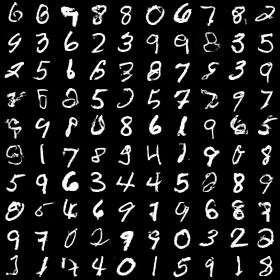
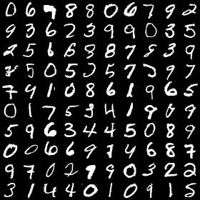
independent
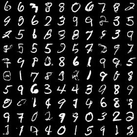
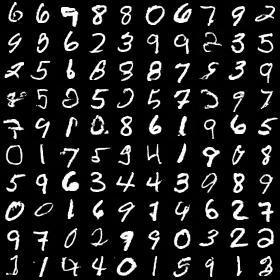
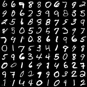
NFEs = 5	NFEs = 10	NFEs = 128

Figure 12: Uncurated MNIST samples.

$\beta=10$
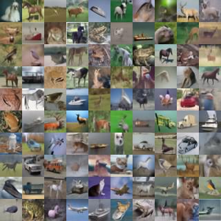
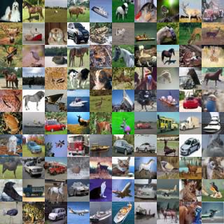
$\beta=20$
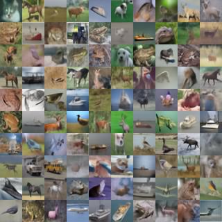
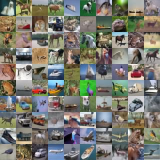
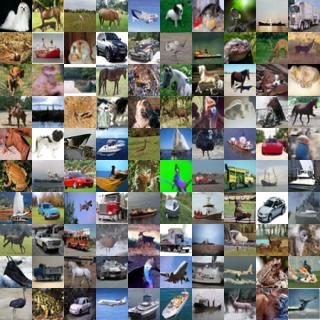
independent
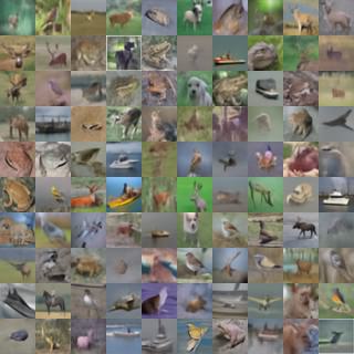
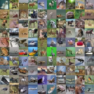
NFEs = 5	NFEs = 9	full sampling

Figure 13: Uncurated CIFAR-10 samples.

References

- Albergo & Vanden-Eijnden (2022) Albergo, M. S. and Vanden-Eijnden, E. Building normalizing flows with stochastic interpolants. arXiv preprint arXiv:2209.15571, 2022.
- Albergo et al. (2023) Albergo, M. S., Boffi, N. M., and Vanden-Eijnden, E. Stochastic interpolants: A unifying framework for flows and diffusions. arXiv preprint arXiv:2303.08797, 2023.
- Bansal et al. (2022) Bansal, A., Borgnia, E., Chu, H.-M., Li, J. S., Kazemi, H., Huang, F., Goldblum, M., Geiping, J., and Goldstein, T. Cold diffusion: Inverting arbitrary image transforms without noise. arXiv preprint arXiv:2208.09392, 2022.
- Benamou & Brenier (2000) Benamou, J.-D. and Brenier, Y. A computational fluid mechanics solution to the monge-kantorovich mass transfer problem. Numerische Mathematik, 84(3):375–393, 2000.
- Brock et al. (2018) Brock, A., Donahue, J., and Simonyan, K. Large scale gan training for high fidelity natural image synthesis. arXiv preprint arXiv:1809.11096, 2018.
- Chen et al. (2018) Chen, R. T., Rubanova, Y., Bettencourt, J., and Duvenaud, D. K. Neural ordinary differential equations. Advances in neural information processing systems, 31, 2018.
- Child (2020) Child, R. Very deep vaes generalize autoregressive models and can outperform them on images. arXiv preprint arXiv:2011.10650, 2020.
- Daras et al. (2022) Daras, G., Delbracio, M., Talebi, H., Dimakis, A. G., and Milanfar, P. Soft diffusion: Score matching for general corruptions. arXiv preprint arXiv:2209.05442, 2022.
- Finlay et al. (2020) Finlay, C., Jacobsen, J.-H., Nurbekyan, L., and Oberman, A. How to train your neural ode: the world of jacobian and kinetic regularization. In International conference on machine learning, pp. 3154–3164. PMLR, 2020.
- Goodfellow et al. (2014) Goodfellow, I., Pouget-Abadie, J., Mirza, M., Xu, B., Warde-Farley, D., Ozair, S., Courville, A., and Bengio, Y. Generative adversarial nets. Advances in neural information processing systems, 27, 2014.
- Gu et al. (2022) Gu, J., Zhai, S., Zhang, Y., Bautista, M. A., and Susskind, J. f-dm: A multi-stage diffusion model via progressive signal transformation. arXiv preprint arXiv:2210.04955, 2022.
- Higgins et al. (2016) Higgins, I., Matthey, L., Pal, A., Burgess, C., Glorot, X., Botvinick, M., Mohamed, S., and Lerchner, A. beta-vae: Learning basic visual concepts with a constrained variational framework. 2016.
- Ho et al. (2020) Ho, J., Jain, A., and Abbeel, P. Denoising diffusion probabilistic models. Advances in Neural Information Processing Systems, 33:6840–6851, 2020.
- Hoogeboom & Salimans (2022) Hoogeboom, E. and Salimans, T. Blurring diffusion models. arXiv preprint arXiv:2209.05557, 2022.
- Karras et al. (2019) Karras, T., Laine, S., and Aila, T. A style-based generator architecture for generative adversarial networks. In Proceedings of the IEEE/CVF conference on computer vision and pattern recognition, pp. 4401–4410, 2019.
- Karras et al. (2020a) Karras, T., Aittala, M., Hellsten, J., Laine, S., Lehtinen, J., and Aila, T. Training generative adversarial networks with limited data. Advances in Neural Information Processing Systems, 33:12104–12114, 2020a.
- Karras et al. (2020b) Karras, T., Laine, S., Aittala, M., Hellsten, J., Lehtinen, J., and Aila, T. Analyzing and improving the image quality of stylegan. In Proceedings of the IEEE/CVF conference on computer vision and pattern recognition, pp. 8110–8119, 2020b.
- Karras et al. (2022) Karras, T., Aittala, M., Aila, T., and Laine, S. Elucidating the design space of diffusion-based generative models. arXiv preprint arXiv:2206.00364, 2022.
- Kelly et al. (2020) Kelly, J., Bettencourt, J., Johnson, M. J., and Duvenaud, D. K. Learning differential equations that are easy to solve. Advances in Neural Information Processing Systems, 33:4370–4380, 2020.
- Kingma & Welling (2013) Kingma, D. P. and Welling, M. Auto-encoding variational bayes. arXiv preprint arXiv:1312.6114, 2013.
- Kingma et al. (2021) Kingma, D. P., Salimans, T., Poole, B., and Ho, J. Variational diffusion models. arXiv preprint arXiv:2107.00630, 2021.
- Lee et al. (2022) Lee, S., Chung, H., Kim, J., and Ye, J. C. Progressive deblurring of diffusion models for coarse-to-fine image synthesis. arXiv preprint arXiv:2207.11192, 2022.
- Lipman et al. (2022) Lipman, Y., Chen, R. T., Ben-Hamu, H., Nickel, M., and Le, M. Flow matching for generative modeling. arXiv preprint arXiv:2210.02747, 2022.
- Liu (2022) Liu, Q. Rectified flow: A marginal preserving approach to optimal transport. arXiv preprint arXiv:2209.14577, 2022.
- Liu et al. (2022) Liu, X., Gong, C., and Liu, Q. Flow straight and fast: Learning to generate and transfer data with rectified flow. arXiv preprint arXiv:2209.03003, 2022.
- Lu et al. (2022) Lu, C., Zhou, Y., Bao, F., Chen, J., Li, C., and Zhu, J. Dpm-solver: A fast ode solver for diffusion probabilistic model sampling in around 10 steps. arXiv preprint arXiv:2206.00927, 2022.
- Luhman & Luhman (2021) Luhman, E. and Luhman, T. Knowledge distillation in iterative generative models for improved sampling speed. arXiv preprint arXiv:2101.02388, 2021.
- Miyato et al. (2018) Miyato, T., Kataoka, T., Koyama, M., and Yoshida, Y. Spectral normalization for generative adversarial networks. arXiv preprint arXiv:1802.05957, 2018.
- Pooladian et al. (2023) Pooladian, A.-A., Ben-Hamu, H., Domingo-Enrich, C., Amos, B., Lipman, Y., and Chen, R. Multisample flow matching: Straightening flows with minibatch couplings. arXiv preprint arXiv:2304.14772, 2023.
- Ramesh et al. (2022) Ramesh, A., Dhariwal, P., Nichol, A., Chu, C., and Chen, M. Hierarchical text-conditional image generation with clip latents. arXiv preprint arXiv:2204.06125, 2022.
- Rezende & Mohamed (2015) Rezende, D. and Mohamed, S. Variational inference with normalizing flows. In International conference on machine learning, pp. 1530–1538. PMLR, 2015.
- Rissanen et al. (2022) Rissanen, S., Heinonen, M., and Solin, A. Generative modelling with inverse heat dissipation. arXiv preprint arXiv:2206.13397, 2022.
- Saharia et al. (2022) Saharia, C., Chan, W., Saxena, S., Li, L., Whang, J., Denton, E., Ghasemipour, S. K. S., Ayan, B. K., Mahdavi, S. S., Lopes, R. G., et al. Photorealistic text-to-image diffusion models with deep language understanding. arXiv preprint arXiv:2205.11487, 2022.
- Salimans & Ho (2022) Salimans, T. and Ho, J. Progressive distillation for fast sampling of diffusion models. arXiv preprint arXiv:2202.00512, 2022.
- Sohl-Dickstein et al. (2015) Sohl-Dickstein, J., Weiss, E., Maheswaranathan, N., and Ganguli, S. Deep unsupervised learning using nonequilibrium thermodynamics. In International Conference on Machine Learning, pp. 2256–2265. PMLR, 2015.
- Song & Ermon (2019) Song, Y. and Ermon, S. Generative modeling by estimating gradients of the data distribution. Advances in Neural Information Processing Systems, 32, 2019.
- Song et al. (2020) Song, Y., Sohl-Dickstein, J., Kingma, D. P., Kumar, A., Ermon, S., and Poole, B. Score-based generative modeling through stochastic differential equations. arXiv preprint arXiv:2011.13456, 2020.
- Vahdat & Kautz (2020) Vahdat, A. and Kautz, J. Nvae: A deep hierarchical variational autoencoder. Advances in Neural Information Processing Systems, 33:19667–19679, 2020.
- Vahdat et al. (2021) Vahdat, A., Kreis, K., and Kautz, J. Score-based generative modeling in latent space. Advances in Neural Information Processing Systems, 34:11287–11302, 2021.
- Vincent (2011) Vincent, P. A connection between score matching and denoising autoencoders. Neural computation, 23(7):1661–1674, 2011.
- Virtanen et al. (2020) Virtanen, P., Gommers, R., Oliphant, T. E., Haberland, M., Reddy, T., Cournapeau, D., Burovski, E., Peterson, P., Weckesser, W., Bright, J., et al. Scipy 1.0: fundamental algorithms for scientific computing in python. Nature methods, 17(3):261–272, 2020.
- Xiao et al. (2021) Xiao, Z., Kreis, K., and Vahdat, A. Tackling the generative learning trilemma with denoising diffusion gans. arXiv preprint arXiv:2112.07804, 2021.
- Zhang & Chen (2021) Zhang, Q. and Chen, Y. Diffusion normalizing flow. Advances in Neural Information Processing Systems, 34:16280–16291, 2021.
- Zhang & Chen (2022) Zhang, Q. and Chen, Y. Fast sampling of diffusion models with exponential integrator. arXiv preprint arXiv:2204.13902, 2022.
- Zhao et al. (2020) Zhao, S., Liu, Z., Lin, J., Zhu, J.-Y., and Han, S. Differentiable augmentation for data-efficient gan training. Advances in Neural Information Processing Systems, 33:7559–7570, 2020.
- Zheng et al. (2022) Zheng, H., Nie, W., Vahdat, A., Azizzadenesheli, K., and Anandkumar, A. Fast sampling of diffusion models via operator learning. arXiv preprint arXiv:2211.13449, 2022.