$L^{2}$ Diffusive Expansion For Neutron Transport Equation

Abstract.

Grazing set singularity leads to a surprising counter-example and breakdown [24] of the classical mathematical theory for $L^{\infty}$ diffusive expansion (1.11) of neutron transport equation with in-flow boundary condition in term of the Knudsen number $\varepsilon$, one of the most classical problems in the kinetic theory. Even though a satisfactory new theory has been established by constructing new boundary layers with favorable $\varepsilon$-geometric correction for convex domains [24, 7, 8, 22, 23], the severe grazing singularity from non-convex domains has prevented any positive mathematical progress. We develop a novel and optimal $L^{2}$ expansion theory for general domain (including non-convex domain) by discovering a surprising $\varepsilon^{\frac{1}{2}}$ gain for the average of remainder.

1. Introduction

1.1. Problem Formulation

We consider the steady neutron transport equation in a three-dimensional $C^{3}$ bounded domain (convex or non-convex) with in-flow boundary condition. In the spatial domain $\Omega\ni x=(x_{1},x_{2},x_{3})$ and the velocity domain $\mathbb{S}^{2}\ni w=(w_{1},w_{2},w_{3})$, the neutron density $u^{\varepsilon}(x,w)$ satisfies

$$\left\{\begin{array}[]{l}\displaystyle w\cdot\nabla_{x}u^{\varepsilon}+\varepsilon^{-1}\Big{(}u^{\varepsilon}-\overline{u^{\varepsilon}}\Big{)}=0\ \ \text{in}\ \ \Omega\times\mathbb{S}^{2},\\ \rule{0.0pt}{11.99998pt}u^{\varepsilon}(x_{0},w)=g(x_{0},w)\ \ \text{for}\ \ w\cdot n<0\ \ \text{and}\ \ x_{0}\in\partial\Omega,\end{array}\right.$$ (1.3)

where $g$ is a given function denoting the in-flow data,

$$\overline{u^{\varepsilon}}(x):=\frac{1}{4\pi}\int_{\mathbb{S}^{2}}u^{\varepsilon}(x,w)\mathrm{d}{w},$$ (1.4)

$n$ is the outward unit normal vector, with the Knudsen number $0<\varepsilon\ll 1$. We intend to study the asymptotic behavior of $u^{\varepsilon}$ as $\varepsilon\rightarrow 0$.

Based on the flow direction, we can divide the boundary $\gamma:=\big{\{}(x_{0},w):\ x_{0}\in\partial\Omega,w\in\mathbb{S}^{2}\big{\}}$ into the incoming boundary $\gamma_{-}$, the outgoing boundary $\gamma_{+}$, and the grazing set $\gamma_{0}$ based on the sign of $w\cdot n(x_{0})$. In particular, the boundary condition of (1.3) is only given on $\gamma_{-}$.

1.2. Normal Chart near Boundary

We follow the approach in [8, 23] to define the geometric quantities, and the details can be found in Section 2.2. For smooth manifold $\partial\Omega$, there exists an orthogonal curvilinear coordinates system $(\iota_{1},\iota_{2})$ such that the coordinate lines coincide with the principal directions at any $x_{0}\in\partial\Omega$. Assume $\partial\Omega$ is parameterized by $\mathbf{r}=\mathbf{r}(\iota_{1},\iota_{2})$. Let the vector length be $L_{i}:=\left|\partial_{\iota_{i}}\mathbf{r}\right|$ and unit vector $\varsigma_{i}:=L_{i}^{-1}\partial_{\iota_{i}}\mathbf{r}$ for $i=1,2$.

Consider the corresponding new coordinate system $(\mu,\iota_{1},\iota_{2})$, where $\mu$ denotes the normal distance to the boundary surface $\partial\Omega$, i.e.

$$x=\mathbf{r}-\mu n.$$ (1.5)

Define the orthogonal velocity substitution for $\mathfrak{w}:=(\varphi,\psi)$ as

$$-w\cdot n=\sin\varphi,\quad w\cdot\varsigma_{1}=\cos\varphi\sin\psi,\quad w\cdot\varsigma_{2}=\cos\varphi\cos\psi.$$ (1.6)

Finally, we define the scaled normal variable $\eta=\dfrac{\mu}{\varepsilon}$, which implies $\dfrac{\partial}{\partial\mu}=\dfrac{1}{\varepsilon}\dfrac{\partial}{\partial\eta}$.

1.3. Asymptotic Expansion and Remainder Equation

We seek a solution to (1.3) in the form

$$u^{\varepsilon}= U+U^{B}+R=\left(U_{0}+\varepsilon U_{1}+\varepsilon^{2}U_{2}\right)+U^{B}_{0}+R,$$ (1.7)

where the interior solution is

$$U(x,w):=U_{0}(x,w)+\varepsilon U_{1}(x,w)+\varepsilon^{2}U_{2}(x,w),$$ (1.8)

and the boundary layer is

$$U^{B}(\eta,\iota_{1},\iota_{2},\mathfrak{w}):=U^{B}_{0}(\eta,\iota_{1},\iota_{2},\mathfrak{w}).$$ (1.9)

Here $U_{0}$, $U_{1}$, $U_{2}$ and $U^{B}_{0}$ are constructed in Section 2.1 and Section 2.2, and $R(x,v)$ is the remainder.

1.4. Literature

The study of the neutron transport equation in bounded domains, has attracted a lot of attention since the dawn of the atomic age. Besides its significance in nuclear sciences and medical imaging, neutron transport equation is usually regarded as a linear prototype of the more important yet more complicated nonlinear Boltzmann equation, and thus, is an ideal starting point to develop new theories and techniques. We refer to [10, 11, 12, 13, 14, 15, 16, 17, 18] for the formal expansion with respect to $\varepsilon$ and explicit solution. The discussion on bounded domain and half-space cases can be found in [5, 4, 3, 1, 2, 19, 20, 21].

The classical boundary layer of neutron transport equation dictates that $U^{B}_{0}(\eta,\iota_{1},\iota_{2},\mathfrak{w})$ satisfies the Milne problem

$$\sin\varphi\frac{\partial U^{B}_{0}}{\partial\eta}+U^{B}_{0}-\overline{U^{B}_{0}}=0.$$ (1.10)

From the formal expansion in $\varepsilon$ (see (2.6)), it is natural to expect the remainder estimate [5]

$$\left\|R\right\|_{L^{\infty}}\lesssim\varepsilon.$$ (1.11)

Even though this is valid for domains with flat boundary, a counter-example is constructed [24] so that (1.11) is invalid for a 2D disk. This is due to the grazing set singularity.

To be more specific, in order to show the remainder estimates (1.11), the higher-order boundary layer expansion $U^{B}_{1}\in L^{\infty}$ is necessary, which further requires $\partial_{\iota_{i}}U^{B}_{0}\in L^{\infty}$. Nevertheless, though $U^{B}_{0}\in L^{\infty}$, it is shown that the normal derivative $\partial_{\eta}U^{B}_{0}$ is singular at the grazing set $\varphi=0$. Furthermore, this singularity $\partial_{\eta}U^{B}_{0}\notin L^{\infty}$ will be transferred to $\partial_{\iota_{i}}U^{B}_{0}\notin L^{\infty}$. A careful construction of boundary data [24] justifies this invalidity, i.e. both the method and result of the boundary layer (1.10) are problematic.

A new construction of boundary layer [24] based on the $\varepsilon$-Milne problem with geometric correction for $\widetilde{U^{B}_{0}}(\eta,\iota_{1},\iota_{2},\mathfrak{w})$

$$\sin\varphi\frac{\partial\widetilde{U^{B}_{0}}}{\partial\eta}-\frac{\varepsilon}{1-\varepsilon\eta}\cos\varphi\frac{\partial\widetilde{U^{B}_{0}}}{\partial\varphi}+\widetilde{U^{B}_{0}}-\overline{\widetilde{U^{B}_{0}}}=0$$ (1.12)

has been shown to provide the satisfactory characterization of the $L^{\infty}$ diffusive expansion in 2D disk domains. With more detailed regularity analysis and boundary layer decomposition techniques for (1.12), such result has been generalized to 2D/3D smooth convex domains [7, 8, 22, 23] and even 2D annulus domain [25].

In non-convex domains, the boundary layer with geometric correction is essentially

$$\sin\varphi\frac{\partial\widetilde{U^{B}_{0}}}{\partial\eta}-\frac{\varepsilon}{1+\varepsilon\eta}\cos\varphi\frac{\partial\widetilde{U^{B}_{0}}}{\partial\varphi}+\widetilde{U^{B}_{0}}-\overline{\widetilde{U^{B}_{0}}}=0$$ (1.13)

Compared to (1.12), this sign flipping dramatically changes the characteristics.

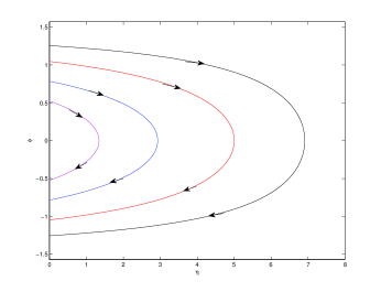
Figure 1. Characteristics in Convex Domains

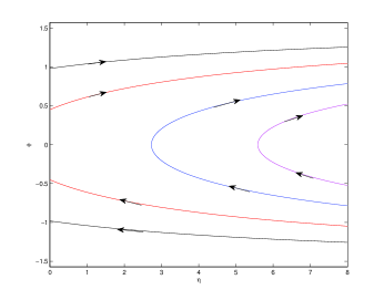
Figure 2. Characteristics in Non-Convex Domains

In Figure 2 and Figure 2 [25], the horizontal direction represents the scaled normal variable $\eta$ and the vertical direction represents the velocity $\varphi$. There exists a “hollow” region in Figure 2 that the characteristics may never track back to the left boundary $\eta=0$ and $\varphi>0$, making the $W^{1,\infty}$ estimates impossible and thus preventing higher-order boundary layer expansion.

In this paper, we will employ a fresh approach to design a cutoff boundary layer without the geometric correction and justify the $L^{2}$ diffusive expansion in smooth non-convex domains.

1.5. Notation and Convention

Let $\left\langle\ \cdot\ ,\ \cdot\ \right\rangle_{w}$ denote the inner product for $w\in\mathbb{S}^{2}$, $\left\langle\ \cdot\ ,\ \cdot\ \right\rangle_{x}$ for $x\in\Omega$, and $\left\langle\ \cdot\ ,\ \cdot\ \right\rangle$ for $(x,w)\in\Omega\times\mathbb{S}^{2}$. Also, let $\left\langle\ \cdot\ ,\ \cdot\ \right\rangle_{\gamma_{\pm}}$ denote the inner product on $\gamma_{\pm}$ with measure $\mathrm{d}\gamma:=\left|w\cdot n\right|\mathrm{d}w\mathrm{d}S_{x}=\left|\sin\varphi\right|\cos\varphi\mathrm{d}\mathfrak{w}\mathrm{d}S_{x}$. Denote the bulk and boundary norms

$$\left\|f\right\|_{L^{2}}:=\left(\iint_{\Omega\times\mathbb{S}^{2}}\left|f(x,w)\right|^{2}\mathrm{d}w\mathrm{d}x\right)^{\frac{1}{2}},\quad\left|f\right|_{L^{2}_{\gamma_{\pm}}}:=\left(\int_{\gamma_{\pm}}\left|f(x,w)\right|^{2}\mathrm{d}\gamma\right)^{\frac{1}{2}}.$$ (1.14)

Define the $L^{\infty}$ norms

$$\left\|f\right\|_{L^{\infty}}:=\operatorname*{ess\,sup}_{(x,w)\in\Omega\times\mathbb{S}^{2}}\big{|}f(x,w)\big{|},\quad\left|f\right|_{L^{\infty}_{\gamma_{\pm}}}:=\operatorname*{ess\,sup}_{(x,w)\in\gamma_{\pm}}\big{|}f(x,w)\big{|}.$$ (1.15)

Let $\left\|\cdot\right\|_{W^{k,p}_{x}}$ denote the usual Sobolev norm for $x\in\Omega$ and $\left|\cdot\right|_{W^{k,p}_{x}}$ for $x\in\partial\Omega$, and $\left\|\cdot\right\|_{W^{k,p}_{x}L^{q}_{w}}$ denote $W^{k,p}$ norm for $x\in\Omega$ and $L^{q}$ norm for $w\in\mathbb{S}^{2}$. The similar notation also applies when we replace $L^{q}$ by $L^{q}_{\gamma}$. When there is no possibility of confusion, we will ignore the $(x,w)$ variables in the norms.

Throughout this paper, $C>0$ denotes a constant that only depends on the domain $\Omega$, but does not depend on the data or $\varepsilon$. It is referred as universal and can change from one inequality to another. We write $a\lesssim b$ to denote $a\leq Cb$ and $a\gtrsim b$ to denote $a\geq Cb$. Also, we write $a\simeq b$ if $a\lesssim b$ and $a\gtrsim b$. We will use $o(1)$ to denote a sufficiently small constant independent of the data.

1.6. Main Results

Theorem 1.1.

Under the assumption

$$\left|g\right|_{W^{3,\infty}L^{\infty}_{\gamma_{-}}}\lesssim 1,$$ (1.16)

there exists a unique solution $u^{\varepsilon}(x,w)\in L^{\infty}(\Omega\times\mathbb{S}^{2})$ to (1.3). Moreover, the solution obeys the estimate

$$\left\|u^{\varepsilon}-U_{0}\right\|_{L^{2}}\lesssim\varepsilon^{\frac{1}{2}}.$$ (1.17)

Here $U_{0}(x)$ satisfies the Laplace equation with Dirichlet boundary condition

$$\left\{\begin{array}[]{l}\Delta_{x}U_{0}(x)=0\ \ \text{in}\ \ \Omega,\\ \rule{0.0pt}{11.99998pt}U_{0}(x_{0})=\Phi_{\infty}(x_{0})\ \ \text{on}\ \ \partial\Omega,\end{array}\right.$$ (1.20)

in which $\Phi_{\infty}(\iota_{1},\iota_{2})=\Phi_{\infty}(x_{0})$ for $x_{0}\in\partial\Omega$ is given by solving the Milne problem for $\Phi(\eta,\iota_{1},\iota_{2},\mathfrak{w})$

$$\left\{\begin{array}[]{l}\sin\varphi\dfrac{\partial\Phi}{\partial\eta}+\Phi-\overline{\Phi}=0,\\ \rule{0.0pt}{11.99998pt}\Phi(0,\iota_{1},\iota_{2},\mathfrak{w})=g(\iota_{1},\iota_{2},\mathfrak{w})\ \ \text{for}\ \ \sin\varphi>0,\\ \rule{0.0pt}{15.00002pt}\displaystyle\lim_{\eta\rightarrow\infty}\Phi(\eta,\iota_{1},\iota_{2},\mathfrak{w})=\Phi_{\infty}(\iota_{1},\iota_{2}).\end{array}\right.$$ (1.24)

Remark 1.2.

In [24, 22, 23] for 2D/3D convex domains, as well as [25] for 2D annulus domain, it is justified that for any $0<\delta\ll 1$

$$\left\|u^{\varepsilon}-\widetilde{U_{0}}-\widetilde{U^{B}_{0}}\right\|_{L^{2}}\lesssim\varepsilon^{\frac{5}{6}-\delta},$$ (1.25)

where $\widetilde{U^{B}_{0}}(\eta,\iota_{1},\iota_{2},\mathfrak{w})$ is the boundary layer with geometric correction defined in (1.12), and $\widetilde{U_{0}}$ is the corresponding interior solution. [21, Theorem 2.1] reveals that the difference between two types of interior solutions

$$\left\|\widetilde{U_{0}}-U_{0}\right\|_{L^{2}}\lesssim\varepsilon^{\frac{2}{3}}.$$ (1.26)

Due to the rescaling $\eta=\varepsilon^{-1}\mu$, for general in-flow boundary data $g$, the boundary layer $\widetilde{U^{B}_{0}}\neq 0$ satisfies

$$\left\|\widetilde{U^{B}_{0}}\right\|_{L^{2}}\simeq\varepsilon^{\frac{1}{2}}.$$ (1.27)

Hence, we conclude that

$$\left\|u^{\varepsilon}-U_{0}\right\|_{L^{2}}\simeq\varepsilon^{\frac{1}{2}}.$$ (1.28)

Therefore, this indicates that (1.17) in Theorem 1.1 achieves the optimal $L^{2}$ bound of the diffusive approximation.

1.7. Methodology

It is well-known that the key of the remainder estimate is to control $\overline{R}$. In a series of work [24, 25, 7, 8, 22, 23] based on a $L^{2}\rightarrow L^{\infty}$ framework, it is shown that

$$\left\|\overline{R}\right\|_{L^{2}}\lesssim\varepsilon^{-1}\left\|R-\overline{R}\right\|_{L^{2}}\lesssim 1$$ (1.29)

combined from the expected energy (entropy production) bound for $\varepsilon^{-1}\left\|R-\overline{R}\right\|_{L^{2}}$. This bound requires the next-order $\varepsilon$ expansion of boundary layer approximation, which is impossible for non-convex domains, and barely possible by the new boundary layer theory with the $\varepsilon$-geometric correction. The key improvement in our work is

$$\left\|\overline{R}\right\|_{L^{2}}\lesssim\varepsilon^{\frac{1}{2}}$$ (1.30)

which is a consequence of the following conservation law for test function $\xi(x)$ satisfying $-\Delta_{x}\xi=\overline{R}$ and $\xi\big{|}_{\partial\Omega}=0$:

$$-\Big{\langle}R,w\cdot\nabla_{x}\xi\Big{\rangle}=-\Big{\langle}R-\overline{R},w\cdot\nabla_{x}\xi\Big{\rangle}=\Big{\langle}S,\xi\Big{\rangle},$$ (1.31)

where $\Big{\langle}\overline{R},w\cdot\nabla_{x}\xi\Big{\rangle}=0$ thanks to the oddness. This conservation law exactly cancels the worst contribution of $\varepsilon^{-1}\left\|R-\overline{R}\right\|_{L^{2}}$ in $\left\|\overline{R}\right\|_{L^{2}}$ estimate, which comes from taking test function $w\cdot\nabla_{x}\xi$

$$\int_{\gamma}R\big{(}w\cdot\nabla_{x}\xi\big{)}(w\cdot n)-\Big{\langle}R,w\cdot\nabla_{x}\big{(}w\cdot\nabla_{x}\xi\big{)}\Big{\rangle}+\varepsilon^{-1}\Big{\langle}R-\overline{R},w\cdot\nabla_{x}\xi\Big{\rangle}=\Big{\langle}S,w\cdot\nabla_{x}\xi\Big{\rangle}.$$ (1.32)

Such a key cancellation produces an extra crucial gain of $\varepsilon^{\frac{1}{2}}$. We then conclude the remainder estimate without any further expansion of the (singular) boundary layer approximation.

In addition, we construct a new cut-off boundary layer near $\varphi=0$ to avoid the singularity, and are able to perform delicate and precise estimates to control the resulting complex forcing term $S$ (see (3.9)–(3.12)), in terms of the desired order $\varepsilon$ for closure.

2. Asymptotic Analysis

2.1. Interior Solution

Inserting (1.8) into (1.3) and comparing the order of $\varepsilon$, following the analysis in [8, 23], we deduce that

$$U_{0}=\overline{U}_{0},\quad\Delta_{x}\overline{U}_{0}=0,$$ (2.1)

$$U_{1}=\overline{U}_{1}-w\cdot\nabla_{x}U_{0},\quad\Delta_{x}\overline{U}_{1}=0,$$ (2.2)

$$U_{2}=\overline{U}_{2}-w\cdot\nabla_{x}U_{1},\quad\Delta_{x}\overline{U}_{2}=0.$$ (2.3)

We need the boundary layer to determine the boundary conditions for $\overline{U}_{0}$, $\overline{U}_{1}$ and $\overline{U}_{2}$.

2.2. Boundary Layer

2.2.1. Geometric Substitutions

The construction of boundary layer requires a local description in a neighborhood of the physical boundary $\partial\Omega$. We follow the procedure in [8, 23]:

Substitution 1: Spacial Substitution

Following the notation in Section 1.2, under the coordinate system $(\mu,\iota_{1},\iota_{2})$, we have

$$w\cdot\nabla_{x}=-(w\cdot n)\frac{\partial}{\partial\mu}-\frac{w\cdot\varsigma_{1}}{L_{1}(\kappa_{1}\mu-1)}\frac{\partial}{\partial\iota_{1}}-\frac{w\cdot\varsigma_{2}}{L_{2}(\kappa_{2}\mu-1)}\frac{\partial}{\partial\iota_{2}},$$ (2.4)

where $\kappa_{i}(\iota_{1},\iota_{2})$ for $i=1,2$ is the principal curvature.

Substitution 2: Velocity Substitution

Under the orthogonal velocity substitution (1.6) for $\varphi\in\left[-\dfrac{\pi}{2},\dfrac{\pi}{2}\right]$ and $\psi\in[-\pi,\pi]$, we have

$$w\cdot\nabla_{x}= \sin\varphi\frac{\partial}{\partial\mu}-\bigg{(}\frac{\sin^{2}\psi}{R_{1}-\mu}+\frac{\cos^{2}\psi}{R_{2}-\mu}\bigg{)}\cos\varphi\frac{\partial}{\partial\varphi}+\frac{\cos\varphi\sin\psi}{L_{1}(1-\kappa_{1}\mu)}\frac{\partial}{\partial\iota_{1}}+\frac{\cos\varphi\cos\psi}{L_{2}(1-\kappa_{2}\mu)}\frac{\partial}{\partial\iota_{2}}$$ (2.5)

$$+\frac{\sin\psi}{R_{1}-\mu}\bigg{\{}\frac{R_{1}\cos\varphi}{L_{1}L_{2}}\bigg{(}\varsigma_{1}\cdot\Big{(}\varsigma_{2}\times\big{(}\partial_{\iota_{1}\iota_{2}}\mathbf{r}\times\varsigma_{2}\big{)}\Big{)}\bigg{)}-\sin\varphi\cos\psi\bigg{\}}\frac{\partial}{\partial\psi}$$

$$-\frac{\cos\psi}{R_{2}-\mu}\bigg{\{}\frac{R_{2}\cos\varphi}{L_{1}L_{2}}\bigg{(}\varsigma_{2}\cdot\Big{(}\varsigma_{1}\times\big{(}\partial_{\iota_{1}\iota_{2}}\mathbf{r}\times\varsigma_{1}\big{)}\Big{)}\bigg{)}-\sin\varphi\sin\psi\bigg{\}}\frac{\partial}{\partial\psi},$$

where $R_{i}=\kappa_{i}^{-1}$ represents the radius of curvature. Note that the Jacobian $\mathrm{d}w=\cos\varphi\mathrm{d}\varphi\mathrm{d}\psi$ will be present when we perform integration.

Substitution 3: Scaling Substitution

Considering the scaled normal variable $\eta=\varepsilon^{-1}\mu$, we have

$$w\cdot\nabla_{x}= \varepsilon^{-1}\sin\varphi\frac{\partial}{\partial\eta}-\bigg{(}\frac{\sin^{2}\psi}{R_{1}-\varepsilon\eta}+\frac{\cos^{2}\psi}{R_{2}-\varepsilon\eta}\bigg{)}\cos\varphi\frac{\partial}{\partial\varphi}+\frac{R_{1}\cos\varphi\sin\psi}{L_{1}(R_{1}-\varepsilon\eta)}\frac{\partial}{\partial\iota_{1}}+\frac{R_{2}\cos\varphi\cos\psi}{L_{2}(R_{2}-\varepsilon\eta)}\frac{\partial}{\partial\iota_{2}}$$ (2.6)

$$+\frac{\sin\psi}{R_{1}-\varepsilon\eta}\bigg{\{}\frac{R_{1}\cos\varphi}{L_{1}L_{2}}\bigg{(}\varsigma_{1}\cdot\Big{(}\varsigma_{2}\times\big{(}\partial_{\iota_{1}\iota_{2}}\mathbf{r}\times\varsigma_{2}\big{)}\Big{)}\bigg{)}-\sin\varphi\cos\psi\bigg{\}}\frac{\partial}{\partial\psi}$$

$$-\frac{\cos\psi}{R_{2}-\varepsilon\eta}\bigg{\{}\frac{R_{2}\cos\varphi}{L_{1}L_{2}}\bigg{(}\varsigma_{2}\cdot\Big{(}\varsigma_{1}\times\big{(}\partial_{\iota_{1}\iota_{2}}\mathbf{r}\times\varsigma_{1}\big{)}\Big{)}\bigg{)}-\sin\varphi\sin\psi\bigg{\}}\frac{\partial}{\partial\psi}.$$

2.2.2. Milne Problem

Let $\Phi(\eta,\iota_{1},\iota_{2},\mathfrak{w})$ be the solution to the Milne problem

$$\sin\varphi\frac{\partial\Phi}{\partial\eta}+\Phi-\overline{\Phi}= 0,\quad\overline{\Phi}(\eta,\iota_{1},\iota_{2})=\frac{1}{4\pi}\int_{-\pi}^{\pi}\int_{-\frac{\pi}{2}}^{\frac{\pi}{2}}\Phi(\eta,\iota_{1},\iota_{2},\mathfrak{w})\cos\varphi\mathrm{d}{\varphi}\mathrm{d}{\psi},$$ (2.7)

with boundary condition

$$\Phi(0,\iota_{1},\iota_{2},\mathfrak{w})=g(\iota_{1},\iota_{2},\mathfrak{w})\ \ \text{for}\ \ \sin\varphi>0.$$ (2.8)

We are interested in the solution that satisfies

$$\lim_{\eta\rightarrow\infty}\Phi(\eta,\iota_{1},\iota_{2},\mathfrak{w})=\Phi_{\infty}(\iota_{1},\iota_{2})$$ (2.9)

for some $\Phi_{\infty}(\iota_{1},\iota_{2})$. Based on [8, Section 4], we have the well-posedness and regularity of (2.7).

Proposition 2.1.

Under the assumption (1.16), there exist $\Phi_{\infty}(\iota_{1},\iota_{2})$ and a unique solution $\Phi$ to (2.7)such that $\Psi:=\Phi-\Phi_{\infty}$ satisfies

$$\left\{\begin{array}[]{l}\sin\varphi\dfrac{\partial\Psi}{\partial\eta}+\Psi-\overline{\Psi}=0,\\ \rule{0.0pt}{11.99998pt}\Psi(0,\iota_{1},\iota_{2},\mathfrak{w})=g(\iota_{1},\iota_{2},\mathfrak{w})-\Phi_{\infty}(\iota_{1},\iota_{2}),\\ \rule{0.0pt}{15.00002pt}\displaystyle\lim_{\eta\rightarrow 0}\Psi(\eta,\iota_{1},\iota_{2},\mathfrak{w})=0,\end{array}\right.$$ (2.13)

and for some constant $K>0$ and any $0<r\leq 3$

$$\left|\Phi_{\infty}\right|_{W^{3,\infty}_{\iota_{1},\iota_{2}}}+\left\|\mathrm{e}^{K\eta}\Psi\right\|_{L^{\infty}}\lesssim 1,$$ (2.14)

$$\left\|\mathrm{e}^{K\eta}\sin\varphi\frac{\partial\Psi}{\partial\eta}\right\|_{L^{\infty}}+\left\|\mathrm{e}^{K\eta}\sin\varphi\frac{\partial\Psi}{\partial\varphi}\right\|_{L^{\infty}}+\left\|\mathrm{e}^{K\eta}\frac{\partial\Psi}{\partial\psi}\right\|_{L^{\infty}}\lesssim 1,$$ (2.15)

$$\left\|\mathrm{e}^{K\eta}\frac{\partial^{r}\Psi}{\partial\iota_{1}^{r}}\right\|_{L^{\infty}}+\left\|\mathrm{e}^{K\eta}\frac{\partial^{r}\Psi}{\partial\iota_{2}^{r}}\right\|_{L^{\infty}}\lesssim 1.$$ (2.16)

Let $\chi(y)\in C^{\infty}(\mathbb{R})$ and $\widetilde{\chi}(y)=1-\chi(y)$ be smooth cut-off functions satisfying $\chi(y)=1$ if $\left|y\right|\leq 1$ and $\chi(y)=0$ if $\left|y\right|\geq 2$. We define the boundary layer

$$U^{B}_{0}(\eta,\iota_{1},\iota_{2},\mathfrak{w}):=\widetilde{\chi}\big{(}\varepsilon^{-1}\varphi\big{)}\chi(\varepsilon\eta)\Psi(\eta,\iota_{1},\iota_{2},\mathfrak{w}).$$ (2.17)

Remark 2.2.

Due to the cutoff in (2.17), we have

$$U^{B}_{0}(0,\iota_{1},\iota_{2},\mathfrak{w})=\widetilde{\chi}\big{(}\varepsilon^{-1}\varphi\big{)}\Big{(}g(\iota_{1},\iota_{2},\mathfrak{w})-\Phi_{\infty}(\iota_{1},\iota_{2})\Big{)}=\widetilde{\chi}\big{(}\varepsilon^{-1}\varphi\big{)}\Psi(0,\iota_{1},\iota_{2},\mathfrak{w}),$$ (2.18)

and

$$\sin\varphi\dfrac{\partial U^{B}_{0}}{\partial\eta}+U^{B}_{0}-\overline{U^{B}_{0}}=-\overline{\widetilde{\chi}\big{(}\varepsilon^{-1}\varphi\big{)}\chi(\varepsilon\eta)\Psi}+\overline{\Psi}\widetilde{\chi}(\varepsilon^{-1}\varphi)\chi(\varepsilon\eta).$$ (2.19)

2.3. Matching Procedure

We plan to enforce the matching condition for $x_{0}\in\partial\Omega$ and $w\cdot n<0$

$$U_{0}(x_{0})+U^{B}_{0}(x_{0},w)= g(x_{0},w)+O(\varepsilon).$$ (2.20)

Considering (2.18), it suffices to require

$$U_{0}(x_{0})=\Phi_{\infty}(x_{0}):=\Phi_{\infty}(\iota_{1},\iota_{2}),$$ (2.21)

which yields

$$U_{0}(x_{0})+\Psi(x_{0},w)= g(x_{0},w).$$ (2.22)

Hence, we obtain

$$U_{0}(x_{0},w)+U^{B}_{0}(x_{0},w)=g(x_{0},w)+\chi\big{(}\varepsilon^{-1}\varphi\big{)}\Psi(0,\iota_{1},\iota_{2},\mathfrak{w}).$$ (2.23)

Construction of $U_{0}$

Based on (2.1) and (2.21), define $U_{0}(x)$ satisfying

$$U_{0}=\overline{U}_{0},\quad\Delta_{x}\overline{U}_{0}=0,\quad U_{0}(x_{0})=\Phi_{\infty}(x_{0}).$$ (2.24)

From standard elliptic estimates [9] and Proposition 2.1, we have for any $s\in[2,\infty)$

$$\left\|U_{0}\right\|_{W^{3+\frac{1}{s},s}}+\left|U_{0}\right|_{W^{3,s}}\lesssim 1.$$ (2.25)

Construction of $U_{1}$

Based on (2.2), define $U_{1}(x,w)$ satisfying

$$U_{1}=\overline{U}_{1}-w\cdot\nabla_{x}U_{0},\quad\Delta_{x}\overline{U}_{1}=0,\quad\overline{U}_{1}(x_{0})=0.$$ (2.26)

From (2.25), we have for any $s\in[2,\infty)$

$$\left\|U_{1}\right\|_{W^{2+\frac{1}{s},s}L^{\infty}}+\left|U_{1}\right|_{W^{2,s}L^{\infty}}\lesssim 1.$$ (2.27)

Construction of $U_{2}$

Based on (2.2), define $U_{2}(x,w)$ satisfying

$$U_{2}=\overline{U}_{2}-w\cdot\nabla_{x}U_{1},\quad\Delta_{x}\overline{U}_{2}=0,\quad\overline{U}_{2}(x_{0})=0.$$ (2.28)

From (2.27), we have for any $s\in[2,\infty)$

$$\left\|U_{2}\right\|_{W^{1+\frac{1}{s},s}L^{\infty}}+\left|U_{2}\right|_{W^{1,s}L^{\infty}}\lesssim 1.$$ (2.29)

Summarizing the above analysis, we have the well-posedness and regularity estimates of the interior solution and boundary layer:

Proposition 2.3.

Under the assumption (1.16), we can construct $U_{0},U_{1},U_{2},U^{B}_{0}$ as in (2.24)(2.26)(2.28)(2.17) satisfying for any $s\in[2,\infty)$

$$\left\|U_{0}\right\|_{W^{3+\frac{1}{s},s}}+\left|U_{0}\right|_{W^{3,s}}\lesssim 1,$$ (2.30)

$$\left\|U_{1}\right\|_{W^{2+\frac{1}{s},s}L^{\infty}}+\left|U_{1}\right|_{W^{2,s}L^{\infty}}\lesssim 1,$$ (2.31)

$$\left\|U_{2}\right\|_{W^{1+\frac{1}{s},s}L^{\infty}}+\left|U_{2}\right|_{W^{1,s}L^{\infty}}\lesssim 1,$$ (2.32)

and for some constant $K>0$ and any $0<r\leq 3$

$$\left\|\mathrm{e}^{K\eta}U^{B}_{0}\right\|_{L^{\infty}}+\left\|\mathrm{e}^{K\eta}\frac{\partial^{r}U^{B}_{0}}{\partial\iota_{1}^{r}}\right\|_{L^{\infty}}+\left\|\mathrm{e}^{K\eta}\frac{\partial^{r}U^{B}_{0}}{\partial\iota_{2}^{r}}\right\|_{L^{\infty}}\lesssim 1.$$ (2.33)

3. Remainder Equation

Denote the approximate solution

$$u_{a}:=\left(U_{0}+\varepsilon U_{1}+\varepsilon^{2}U_{2}\right)+U^{B}_{0}.$$ (3.1)

Inserting (1.7) into (1.3), we have

$$w\cdot\nabla_{x}\big{(}u_{a}+R\big{)}+\varepsilon^{-1}\Big{(}u_{a}+R\Big{)}-\varepsilon^{-1}\Big{(}\overline{u_{a}}+\overline{R}\Big{)}=0,\quad\big{(}u_{a}+R\big{)}\Big{|}_{\gamma_{-}}=g,$$ (3.2)

which yields

$$w\cdot\nabla_{x}R+\varepsilon^{-1}\Big{(}R-\overline{R}\Big{)}=-w\cdot\nabla_{x}u_{a}-\varepsilon^{-1}\Big{(}u_{a}-\overline{u_{a}}\Big{)},\quad R\Big{|}_{\gamma_{-}}=\big{(}g-u_{a}\big{)}\Big{|}_{\gamma_{-}}.$$ (3.3)

3.1. Formulation of Remainder Equation

We consider the remainder equation

$$\left\{\begin{array}[]{l}\displaystyle w\cdot\nabla_{x}R+\varepsilon^{-1}\Big{(}R-\overline{R}\Big{)}=S\ \ \text{in}\ \ \Omega\times\mathbb{S}^{2},\\ \rule{0.0pt}{11.99998pt}R(x_{0},w)=h(x_{0},w)\ \ \text{for}\ \ w\cdot n<0\ \ \text{and}\ \ x_{0}\in\partial\Omega,\end{array}\right.$$ (3.6)

where $\displaystyle\overline{R}(x)=\frac{1}{4\pi}\int_{\mathbb{S}^{2}}R(x,w)\mathrm{d}{w}$. Here the boundary data $h$ is given by

$$h:=-\varepsilon w\cdot\nabla_{x}U_{0}-\varepsilon^{2}w\cdot\nabla_{x}U_{1}-\chi\big{(}\varepsilon^{-1}\varphi\big{)}\Psi(0),$$ (3.7)

and the source term $S$ is given by

$$S:=S_{0}+S_{1}+S_{2}+S_{3},$$ (3.8)

where

$$S_{0}:= -\varepsilon^{2}w\cdot\nabla_{x}U_{2},$$ (3.9)

$$S_{1}:= \bigg{(}\dfrac{\sin^{2}\psi}{R_{1}-\varepsilon\eta}+\dfrac{\cos^{2}\psi}{R_{2}-\varepsilon\eta}\bigg{)}\cos\varphi\dfrac{\partial U^{B}_{0}}{\partial\varphi},$$ (3.10)

$$S_{2}:= \varepsilon^{-1}\sin\phi\widetilde{\chi}\big{(}\varepsilon^{-1}\varphi\big{)}\frac{\partial\chi(\varepsilon\eta)}{\partial\eta}\Psi+\frac{R_{1}\cos\varphi\sin\psi}{L_{1}(R_{1}-\varepsilon\eta)}\frac{\partial U^{B}_{0}}{\partial\iota_{1}}+\frac{R_{2}\cos\varphi\cos\psi}{L_{2}(R_{2}-\varepsilon\eta)}\frac{\partial U^{B}_{0}}{\partial\iota_{2}}$$ (3.11)

$$+\frac{\sin\psi}{R_{1}-\varepsilon\eta}\bigg{\{}\frac{R_{1}\cos\varphi}{L_{1}L_{2}}\bigg{(}\varsigma_{1}\cdot\Big{(}\varsigma_{2}\times\big{(}\partial_{\iota_{1}\iota_{2}}\mathbf{r}\times\varsigma_{2}\big{)}\Big{)}\bigg{)}-\sin\varphi\cos\psi\bigg{\}}\frac{\partial U^{B}_{0}}{\partial\psi}$$

$$-\frac{\cos\psi}{R_{2}-\varepsilon\eta}\bigg{\{}\frac{R_{2}\cos\varphi}{L_{1}L_{2}}\bigg{(}\varsigma_{2}\cdot\Big{(}\varsigma_{1}\times\big{(}\partial_{\iota_{1}\iota_{2}}\mathbf{r}\times\varsigma_{1}\big{)}\Big{)}\bigg{)}-\sin\varphi\sin\psi\bigg{\}}\frac{\partial U^{B}_{0}}{\partial\psi},$$

$$S_{3}:= \varepsilon^{-1}\bigg{(}\overline{\widetilde{\chi}\big{(}\varepsilon^{-1}\varphi\big{)}\chi(\varepsilon\eta)\Psi}-\overline{\Psi}\widetilde{\chi}\big{(}\varepsilon^{-1}\varphi\big{)}\chi(\varepsilon\eta)\bigg{)}.$$ (3.12)

3.2. Weak Formulation

Lemma 3.1 (Green’s Identity, Lemma 2.2 of [6]).

Assume $f(x,w),\ g(x,w)\in L^{2}(\Omega\times\mathbb{S}^{2})$ and $w\cdot\nabla_{x}f,\ w\cdot\nabla_{x}g\in L^{2}(\Omega\times\mathbb{S}^{2})$ with $f,\ g\in L^{2}_{\gamma}$. Then

$$\iint_{\Omega\times\mathbb{S}^{2}}\Big{(}\big{(}w\cdot\nabla_{x}f\big{)}g+\big{(}w\cdot\nabla_{x}g\big{)}f\Big{)}\mathrm{d}{x}\mathrm{d}{w}=\int_{\gamma}fg(w\cdot n)=\int_{\gamma_{+}}fg\mathrm{d}{\gamma}-\int_{\gamma_{-}}fg\mathrm{d}{\gamma}.$$ (3.13)

Using Lemma 3.1, we can derive the weak formulation of (3.6). For any test function $\mathfrak{g}(x,w)\in L^{2}(\Omega\times\mathbb{S}^{2})$ with $w\cdot\nabla_{x}\mathfrak{g}\in L^{2}(\Omega\times\mathbb{S}^{2})$ with $\mathfrak{g}\in L^{2}_{\gamma}$, we have

$$\int_{\gamma}R\mathfrak{g}(w\cdot n)-\iint_{\Omega\times\mathbb{S}^{2}}R\big{(}w\cdot\nabla_{x}\mathfrak{g}\big{)}+\varepsilon^{-1}\iint_{\Omega\times\mathbb{S}^{2}}\Big{(}R-\overline{R}\Big{)}\mathfrak{g}=\iint_{\Omega\times\mathbb{S}^{2}}S\mathfrak{g}.$$ (3.14)

3.3. Estimates of Boundary and Source Terms

Lemma 3.2.

Under the assumption (1.16), for $h$ defined in (3.7), we have

$$\left|h\right|_{L^{2}_{\gamma_{-}}}\lesssim\varepsilon.$$ (3.15)

Proof.

Based on Proposition 2.3, we have

$$\left|\varepsilon w\cdot\nabla_{x}U_{0}\right|_{L^{2}_{\gamma_{-}}}+\left|\varepsilon^{2}w\cdot\nabla_{x}U_{1}\right|_{L^{2}_{\gamma_{-}}}\lesssim\varepsilon.$$ (3.16)

Noting the cutoff $\chi\big{(}\varepsilon^{-1}\varphi\big{)}$ restricts the support to $\left|\varphi\right|\lesssim\varepsilon$ and $\mathrm{d}\gamma$ measure contributes an extra $\sin\varphi$, we have

$$\left|\chi\big{(}\varepsilon^{-1}\varphi\big{)}\Psi(0)\right|_{L^{2}_{\gamma_{-}}}\lesssim\varepsilon.$$ (3.17)

Hence, our result follows. ∎

Lemma 3.3.

Under the assumption (1.16), for $S_{0}$ defined in (3.9), we have

$$\left\|S_{0}\right\|_{L^{2}}\lesssim\varepsilon^{2}.$$ (3.18)

Proof.

This follows from Proposition 2.3. ∎

Lemma 3.4.

Under the assumption (1.16), for $S_{1}$ defined in (3.10), we have

$$\left\|\big{(}1+\eta\big{)}S_{1}\right\|_{L^{2}}\lesssim 1.$$ (3.19)

Also, for the boundary layer $U^{B}_{0}$ defined in (2.17), we have

$$\left\|\big{(}1+\eta\big{)}U^{B}_{0}\right\|_{L^{2}}\lesssim\varepsilon^{\frac{1}{2}},\quad\left\|\big{(}1+\eta\big{)}U^{B}_{0}\right\|_{L^{2}_{x}L^{1}_{w}}\lesssim\varepsilon^{\frac{1}{2}},$$ (3.20)

and

$$\left|\Big{\langle}\big{(}1+\eta\big{)}S_{1},g\Big{\rangle}\right| \lesssim\left\|\big{(}1+\eta\big{)}\left\langle v\right\rangle^{2}U^{B}_{0}\right\|_{L^{2}}\left\|\nabla_{w}g\right\|_{L^{2}}\lesssim\varepsilon^{\frac{1}{2}}\left\|\nabla_{w}g\right\|_{L^{2}}.$$ (3.21)

Proof.

We split

$$S_{1}=S_{11}+S_{12}:= \bigg{(}\dfrac{\sin^{2}\psi}{R_{1}-\varepsilon\eta}+\dfrac{\cos^{2}\psi}{R_{2}-\varepsilon\eta}\bigg{)}\cos\varphi\dfrac{\partial\Psi}{\partial\varphi}\widetilde{\chi}\big{(}\varepsilon^{-1}\varphi\big{)}\chi(\varepsilon\eta)$$ (3.22)

$$+\bigg{(}\dfrac{\sin^{2}\psi}{R_{1}-\varepsilon\eta}+\dfrac{\cos^{2}\psi}{R_{2}-\varepsilon\eta}\bigg{)}\cos\varphi\dfrac{\partial\widetilde{\chi}\big{(}\varepsilon^{-1}\varphi\big{)}}{\partial\varphi}\chi(\varepsilon\eta)\Psi.$$

Note that $S_{11}$ is nonzero only when $\left|\varphi\right|\geq\varepsilon$ and thus based on Proposition 2.1, we know $\left|\dfrac{\partial\Psi}{\partial\varphi}\right|\leq\left|\sin\varphi\right|^{-1}\left|\Psi\right|\lesssim\varepsilon^{-1}$. Hence, using $\mathrm{d}\mu=\varepsilon\mathrm{d}\eta$, we have

$$\left\|S_{11}\right\|_{L^{2}}\lesssim \left(\iint_{\left|\varphi\right|\geq\varepsilon}\left|\dfrac{\partial\Psi}{\partial\varphi}\right|^{2}\mathrm{d}\varphi\mathrm{d}\mu\right)^{\frac{1}{2}}\lesssim\left(\iint_{\left|\varphi\right|\geq\varepsilon}\left|\sin\varphi\right|^{-2}\left|\Psi\right|^{2}\mathrm{d}\varphi\mathrm{d}\mu\right)^{\frac{1}{2}}$$ (3.23)

$$\lesssim \left(\iint_{\left|\varphi\right|\geq\varepsilon}\left|\sin\varphi\right|^{-2}\mathrm{e}^{-2K\eta}\mathrm{d}\varphi\mathrm{d}\mu\right)^{\frac{1}{2}}\lesssim\left(\varepsilon\iint_{\left|\varphi\right|\geq\varepsilon}\left|\sin\varphi\right|^{-2}\mathrm{e}^{-2K\eta}\mathrm{d}\varphi\mathrm{d}\eta\right)^{\frac{1}{2}}\lesssim\left(\varepsilon\varepsilon^{-1}\right)^{\frac{1}{2}}=1.$$

Noticing $\dfrac{\partial\widetilde{\chi}\big{(}\varepsilon^{-1}\varphi\big{)}}{\partial\varphi}=\varepsilon^{-1}\widetilde{\chi}^{\prime}\big{(}\varepsilon^{-1}\varphi\big{)}$, and $\widetilde{\chi}^{\prime}\big{(}\varepsilon^{-1}\varphi\big{)}$ is nonzero only when $\varepsilon<\left|\varphi\right|<2\varepsilon$, based on Proposition 2.1, we have

$$\left\|S_{12}\right\|_{L^{2}}\lesssim \varepsilon^{-1}\left(\iint_{\varepsilon<\left|\varphi\right|<2\varepsilon}\left|\Psi\right|^{2}\mathrm{d}\varphi\mathrm{d}\mu\right)^{\frac{1}{2}}\lesssim\varepsilon^{-1}\left(\iint_{\varepsilon<\left|\varphi\right|<2\varepsilon}\mathrm{e}^{-2K\eta}\mathrm{d}\varphi\mathrm{d}\mu\right)^{\frac{1}{2}}$$ (3.24)

$$\lesssim \varepsilon^{-1}\left(\varepsilon\iint_{\varepsilon<\left|\varphi\right|<2\varepsilon}\mathrm{e}^{-2K\eta}\mathrm{d}\varphi\mathrm{d}\eta\right)^{\frac{1}{2}}\lesssim\varepsilon^{-1}\left(\varepsilon\varepsilon\right)^{\frac{1}{2}}=1.$$

Collecting (3.23) and (3.24), we have (3.19). Note that $\mathrm{e}^{-K\eta}$ will suppress the growth from the pre-factor $1+\eta$.

(3.20) comes from Proposition 2.1. Then we turn to (3.21). The most difficult term in $\big{|}\left\langle S_{1},g\right\rangle\big{|}$ is essentially $\left|\left\langle\dfrac{\partial U^{B}_{0}}{\partial\varphi},g\right\rangle\right|$. Integration by parts with respect to $\varphi$ implies

$$\left|\left\langle\frac{\partial U^{B}_{0}}{\partial\varphi},g\right\rangle\right|\lesssim \left|\left\langle U^{B}_{0},\frac{\partial g}{\partial\varphi}\right\rangle\right|\lesssim\left\|U^{B}_{0}\right\|_{L^{2}}\left\|\frac{\partial g}{\partial\varphi}\right\|_{L^{2}}.$$ (3.25)

From (1.6) and $\dfrac{\partial x}{\partial\varphi}=0$, we know the substitution $(\mu,\iota_{1},\iota_{2},w)\rightarrow(\mu,\iota_{1},\iota_{2},\mathfrak{w})$ implies

$$-\dfrac{\partial w}{\partial\varphi}\cdot n=\cos\varphi,\quad\dfrac{\partial w}{\partial\varphi}\cdot\varsigma_{1}=-\sin\varphi\sin\psi,\quad\dfrac{\partial w}{\partial\varphi}\cdot\varsigma_{2}=-\sin\varphi\cos\psi.$$ (3.26)

Hence, we know $\left|\dfrac{\partial w}{\partial\varphi}\right|\lesssim 1$, and thus

$$\left|\frac{\partial g}{\partial\varphi}\right|\lesssim\left|\nabla_{w}g\right|\left|\frac{\partial w}{\partial\varphi}\right|\lesssim\left|\nabla_{w}g\right|.$$ (3.27)

Hence, we know that

$$\left|\left\langle\frac{\partial U^{B}_{0}}{\partial\varphi},g\right\rangle\right|\lesssim \left\|U^{B}_{0}\right\|_{L^{2}}\left\|\nabla_{w}g\right\|_{L^{2}}\lesssim\varepsilon^{\frac{1}{2}}\left\|\nabla_{w}g\right\|_{L^{2}}.$$ (3.28)

∎

Lemma 3.5.

Under the assumption (1.16), for $S_{2}$ defined in (3.11), we have

$$\left\|\big{(}1+\eta\big{)}S_{2}\right\|_{L^{2}}\lesssim\varepsilon^{\frac{1}{2}},\quad\left\|\big{(}1+\eta\big{)}S_{2}\right\|_{L^{2}_{x}L^{1}_{w}}\lesssim\varepsilon^{\frac{1}{2}}.$$ (3.29)

Proof.

Notice that $\left|\varepsilon^{-1}\sin\phi\widetilde{\chi}\big{(}\varepsilon^{-1}\varphi\big{)}\dfrac{\partial\chi(\varepsilon\eta)}{\partial\eta}\right|\lesssim 1$. Based on Proposition 2.1 and Proposition 2.3, we directly bound

$$\left\|S_{2}\right\|_{L^{2}}\lesssim \left(\iint\bigg{(}\left|\Phi\right|^{2}+\left|\dfrac{\partial\Phi}{\partial\iota_{1}}\right|^{2}+\left|\dfrac{\partial\Phi}{\partial\iota_{2}}\right|^{2}+\left|\dfrac{\partial\Phi}{\partial\psi}\right|^{2}\bigg{)}\mathrm{d}\varphi\mathrm{d}\mu\right)^{\frac{1}{2}}$$ (3.30)

$$\lesssim \left(\iint\mathrm{e}^{-2K\eta}\mathrm{d}\varphi\mathrm{d}\mu\right)^{\frac{1}{2}}\lesssim\left(\varepsilon\iint\mathrm{e}^{-2K\eta}\mathrm{d}\varphi\mathrm{d}\eta\right)^{\frac{1}{2}}\lesssim\varepsilon^{\frac{1}{2}}.$$

Then the $L^{2}_{x}L^{1}_{w}$ estimate follows from a similar argument noting that there is no rescaling in $w$ variables. ∎

Lemma 3.6.

Under the assumption (1.16), for $S_{3}$ defined in (3.12), we have

$$\left\|\big{(}1+\eta\big{)}S_{3}\right\|_{L^{2}}\lesssim 1,\quad\left\|\big{(}1+\eta\big{)}S_{3}\right\|_{L^{2}_{x}L^{1}_{w}}\lesssim\varepsilon^{\frac{1}{2}}.$$ (3.31)

Proof.

Using $\chi=1-\widetilde{\chi}$, we split

$$S_{3}=S_{31}+S_{32}:= \varepsilon^{-1}\overline{\Psi}\chi\big{(}\varepsilon^{-1}\varphi\big{)}\chi(\varepsilon\eta)-\varepsilon^{-1}\overline{\chi\big{(}\varepsilon^{-1}\varphi\big{)}\chi(\varepsilon\eta)\Psi}.$$ (3.32)

Noting that $S_{31}$ is nonzero only when $\left|\varphi\right|\leq\varepsilon$, based on Proposition 2.1, we have

$$\left\|S_{31}\right\|_{L^{2}}\lesssim \left(\iint_{\left|\varphi\right|\leq\varepsilon}\left|\varepsilon^{-1}\overline{\Psi}\right|^{2}\mathrm{d}\varphi\mathrm{d}\mu\right)^{\frac{1}{2}}\lesssim\left(\varepsilon^{-2}\iint_{\left|\varphi\right|\leq\varepsilon}\mathrm{e}^{-2K\eta}\mathrm{d}\varphi\mathrm{d}\mu\right)^{\frac{1}{2}}$$ (3.33)

$$\lesssim \left(\varepsilon^{-1}\iint_{\left|\varphi\right|\leq\varepsilon}\mathrm{e}^{-2K\eta}\mathrm{d}\varphi\mathrm{d}\eta\right)^{\frac{1}{2}}\lesssim\left(\varepsilon^{-1}\varepsilon\right)^{\frac{1}{2}}\lesssim 1.$$

Analogously, noting that $S_{32}$ contains $w$ integral, we have

$$\left\|S_{32}\right\|_{L^{2}}\lesssim \left(\iint\left|\varepsilon^{-1}\overline{\Psi\chi(\varepsilon^{-1}\varphi)}\right|^{2}\mathrm{d}\varphi\mathrm{d}\mu\right)^{\frac{1}{2}}\lesssim\left(\varepsilon^{-2}\iint\left|\int_{\left|\varphi\right|\leq\varepsilon}\Psi\mathrm{d}\varphi\right|^{2}\mathrm{d}\varphi\mathrm{d}\mu\right)^{\frac{1}{2}}$$ (3.34)

$$\lesssim \left(\varepsilon^{-2}\iint\left|\int_{\left|\varphi\right|\leq\varepsilon}\mathrm{e}^{-K\eta}\mathrm{d}\varphi\right|^{2}\mathrm{d}\varphi\mathrm{d}\mu\right)^{\frac{1}{2}}\lesssim\left(\varepsilon^{-2}\iint\varepsilon^{2}\mathrm{e}^{-2K\eta}\mathrm{d}\varphi\mathrm{d}\mu\right)^{\frac{1}{2}}$$

$$\lesssim \left(\iint\mathrm{e}^{-2K\eta}\mathrm{d}\varphi\mathrm{d}\mu\right)^{\frac{1}{2}}\lesssim\left(\varepsilon\iint\mathrm{e}^{-2K\eta}\mathrm{d}\varphi\mathrm{d}\eta\right)^{\frac{1}{2}}\lesssim\varepsilon^{\frac{1}{2}}.$$

Collecting (3.33) and (3.34), we have the $L^{2}$ estimate. Similarly, we derive the $L^{2}_{x}L^{1}_{w}$ bound:

$$\left\|S_{31}\right\|_{L^{2}_{x}L^{1}_{w}}\lesssim \left(\int\bigg{(}\int_{\left|\varphi\right|\leq\varepsilon}\left|\varepsilon^{-1}\overline{\Psi}\right|\mathrm{d}\varphi\bigg{)}^{2}\mathrm{d}\mu\right)^{\frac{1}{2}}\lesssim\left(\int\mathrm{e}^{-2K\eta}\mathrm{d}\mu\right)^{\frac{1}{2}}\lesssim\left(\varepsilon\int\mathrm{e}^{-2K\eta}\mathrm{d}\eta\right)^{\frac{1}{2}}\lesssim\varepsilon^{\frac{1}{2}},$$ (3.35)

$$\left\|S_{32}\right\|_{L^{2}_{x}L^{1}_{w}}\lesssim \left(\int\bigg{(}\int\left|\varepsilon^{-1}\overline{\Psi\chi(\varepsilon^{-1}\varphi)}\right|\mathrm{d}\varphi\bigg{)}^{2}\mathrm{d}\mu\right)^{\frac{1}{2}}\lesssim\left(\varepsilon^{-2}\int\bigg{(}\int\left|\int_{\left|\varphi\right|\leq\varepsilon}\Psi\mathrm{d}\varphi\right|\mathrm{d}\varphi\bigg{)}^{2}\mathrm{d}\mu\right)^{\frac{1}{2}}$$ (3.36)

$$\lesssim \left(\varepsilon^{-2}\int\bigg{(}\int\varepsilon\mathrm{e}^{-K\eta}\mathrm{d}\varphi\bigg{)}^{2}\mathrm{d}\mu\right)^{\frac{1}{2}}\lesssim\left(\int\mathrm{e}^{-2K\eta}\mathrm{d}\mu\right)^{\frac{1}{2}}\lesssim\left(\varepsilon\int\mathrm{e}^{-2K\eta}\mathrm{d}\eta\right)^{\frac{1}{2}}\lesssim\varepsilon^{\frac{1}{2}}.$$

∎

4. Remainder Estimate

4.1. Basic Energy Estimate

Lemma 4.1.

Under the assumption (1.16), we have

$$\varepsilon^{-1}\left|R\right|_{L^{2}_{\gamma_{+}}}^{2}+\varepsilon^{-2}\left\|R-\overline{R}\right\|_{L^{2}}^{2}\lesssim o(1)\varepsilon^{-1}\left\|\overline{R}\right\|_{L^{2}}^{2}+1.$$ (4.1)

Proof.

Taking $\mathfrak{g}=\varepsilon^{-1}R$ in (3.14), we obtain

$$\frac{\varepsilon^{-1}}{2}\int_{\gamma}\left|R\right|^{2}(w\cdot n)+\varepsilon^{-2}\Big{\langle}R,R-\overline{R}\Big{\rangle}=\varepsilon^{-1}\Big{\langle}R,S\Big{\rangle}.$$ (4.2)

Then using the orthogonality of $\overline{R}$ and $R-\overline{R}$, we have

$$\frac{\varepsilon^{-1}}{2}\left|R\right|_{L^{2}_{\gamma_{+}}}^{2}+\varepsilon^{-2}\left\|R-\overline{R}\right\|_{L^{2}}^{2}=\varepsilon^{-1}\Big{\langle}R,S\Big{\rangle}+\frac{\varepsilon^{-1}}{2}\left|h\right|_{L^{2}_{\gamma_{-}}}^{2}.$$ (4.3)

Using Lemma 3.2, we know

$$\varepsilon^{-1}\left|R\right|_{L^{2}_{\gamma_{+}}}^{2}+\varepsilon^{-2}\left\|R-\overline{R}\right\|_{L^{2}}^{2}\lesssim\varepsilon+\varepsilon^{-1}\Big{\langle}R,S_{0}+S_{1}+S_{2}+S_{3}\Big{\rangle}.$$ (4.4)

Using Lemma 3.3, we have

$$\left|\varepsilon^{-1}\Big{\langle}R,S_{0}\Big{\rangle}\right|\lesssim\varepsilon^{-1}\left\|R\right\|_{L^{2}}\left\|S_{0}\right\|_{L^{2}}\lesssim\varepsilon\left\|R\right\|_{L^{2}}\lesssim o(1)\left\|R\right\|_{L^{2}}^{2}+\varepsilon^{2}.$$ (4.5)

Using Lemma 3.4, Lemma 3.5 and Lemma 3.6, we have

$$\left|\varepsilon^{-1}\Big{\langle}R-\overline{R},S_{1}+S_{2}+S_{3}\Big{\rangle}\right|\lesssim \varepsilon^{-1}\left\|R-\overline{R}\right\|_{L^{2}}\left\|S_{1}+S_{2}+S_{3}\right\|_{L^{2}}$$ (4.6)

$$\lesssim \varepsilon^{-1}\left\|R-\overline{R}\right\|_{L^{2}}\lesssim o(1)\varepsilon^{-2}\left\|R-\overline{R}\right\|_{L^{2}}^{2}+1.$$

Finally, we turn to $\varepsilon^{-1}\Big{\langle}\overline{R},S_{1}+S_{2}+S_{3}\Big{\rangle}$. For $S_{1}$, we integrate by parts with respect to $\varphi$ and use Lemma 3.4 to obtain

$$\left|\varepsilon^{-1}\Big{\langle}\overline{R},S_{1}\Big{\rangle}\right|= \varepsilon^{-1}\left|\left\langle\overline{R},\bigg{(}\dfrac{\sin^{2}\psi}{R_{1}-\varepsilon\eta}+\dfrac{\cos^{2}\psi}{R_{2}-\varepsilon\eta}\bigg{)}\cos\varphi\dfrac{\partial U^{B}_{0}}{\partial\varphi}\right\rangle\right|$$ (4.7)

$$= \varepsilon^{-1}\left|\left\langle\overline{R},\bigg{(}\dfrac{\sin^{2}\psi}{R_{1}-\varepsilon\eta}+\dfrac{\cos^{2}\psi}{R_{2}-\varepsilon\eta}\bigg{)}U^{B}_{0}\sin\varphi\right\rangle\right|$$

$$\lesssim \varepsilon^{-1}\left\|\overline{R}\right\|_{L^{2}}\left\|U^{B}_{1}\right\|_{L^{2}_{x}L^{1}_{w}}\lesssim\varepsilon^{-\frac{1}{2}}\left\|\overline{R}\right\|_{L^{2}}\lesssim o(1)\varepsilon^{-1}\left\|\overline{R}\right\|_{L^{2}}^{2}+1.$$

Also, Lemma 3.5 and Lemma 3.6 yield

$$\left|\varepsilon^{-1}\Big{\langle}\overline{R},S_{2}+S_{3}\Big{\rangle}\right|\lesssim \varepsilon^{-1}\left\|\overline{R}\right\|_{L^{2}}\Big{(}\left\|S_{2}\right\|_{L^{2}_{x}L^{1}_{w}}+\left\|S_{3}\right\|_{L^{2}_{x}L^{1}_{w}}\Big{)}\lesssim\varepsilon^{-\frac{1}{2}}\left\|\overline{R}\right\|_{L^{2}}\lesssim o(1)\varepsilon^{-1}\left\|\overline{R}\right\|_{L^{2}}^{2}+1.$$ (4.8)

Collecting (4.5)(4.6)(4.7)(4.8), we obtain

$$\left|\varepsilon^{-1}\Big{\langle}R,S_{0}+S_{1}+S_{2}+S_{3}\Big{\rangle}\right|\lesssim o(1)\varepsilon^{-2}\left\|R-\overline{R}\right\|_{L^{2}}^{2}+o(1)\varepsilon^{-1}\left\|R\right\|_{L^{2}}^{2}+1.$$ (4.9)

Combining (4.9) and (4.4), we have (4.1). ∎

4.2. Kernel Estimate

Lemma 4.2.

Under the assumption (1.16), we have

$$\left\|\overline{R}\right\|_{L^{2}}^{2}\lesssim\left\|R-\overline{R}\right\|_{L^{2}}^{2}+\left|R\right|_{L^{2}_{\gamma_{+}}}^{2}+\varepsilon.$$ (4.10)

Proof.

Denote $\xi(x)$ satisfying

$$\left\{\begin{array}[]{l}-\Delta_{x}\xi=\overline{R}\ \ \text{in}\ \ \Omega,\\ \rule{0.0pt}{11.99998pt}\xi(x_{0})=0\ \ \text{on}\ \ \partial\Omega.\end{array}\right.$$ (4.13)

Based on standard elliptic estimates and trace estimates, we have

$$\left\|\xi\right\|_{H^{2}}+\left|\xi\right|_{H^{\frac{3}{2}}}\lesssim\left\|\overline{R}\right\|_{L^{2}}.$$ (4.14)

Taking $\mathfrak{g}=\xi$ in (3.14), we have

$$\int_{\gamma}R\xi(w\cdot n)-\Big{\langle}R,w\cdot\nabla_{x}\xi\Big{\rangle}+\varepsilon^{-1}\Big{\langle}R-\overline{R},\xi\Big{\rangle}=\Big{\langle}S,\xi\Big{\rangle}.$$ (4.15)

Using oddness, orthogonality and $\xi\big{|}_{\partial\Omega}=0$, we obtain (1.31).

Then taking $\mathfrak{g}=w\cdot\nabla_{x}\xi$ in (3.14), we obtain (1.32).

Adding $\varepsilon^{-1}\times$(1.31) and (1.32) to eliminate $\varepsilon^{-1}\Big{\langle}R-\overline{R},w\cdot\nabla_{x}\xi\Big{\rangle}$, we obtain

$$\int_{\gamma}R\big{(}w\cdot\nabla_{x}\xi\big{)}(w\cdot n)-\Big{\langle}R,w\cdot\nabla_{x}\big{(}w\cdot\nabla_{x}\xi\big{)}\Big{\rangle}= \varepsilon^{-1}\Big{\langle}S,\xi\Big{\rangle}+\Big{\langle}S,w\cdot\nabla_{x}\xi\Big{\rangle}.$$ (4.16)

Notice that

$$-\Big{\langle}R,w\cdot\nabla_{x}\big{(}w\cdot\nabla_{x}\xi\big{)}\Big{\rangle}= -\Big{\langle}\overline{R},w\cdot\nabla_{x}\big{(}w\cdot\nabla_{x}\xi\big{)}\Big{\rangle}-\Big{\langle}R-\overline{R},w\cdot\nabla_{x}\big{(}w\cdot\nabla_{x}\xi\big{)}\Big{\rangle},$$ (4.17)

where (4.14) and Cauchy’s inequality yield

$$-\Big{\langle}\overline{R},w\cdot\nabla_{x}\big{(}w\cdot\nabla_{x}\xi\big{)}\Big{\rangle}\simeq \left\|\overline{R}\right\|_{L^{2}}^{2},$$ (4.18)

$$\left|\Big{\langle}R-\overline{R},w\cdot\nabla_{x}\big{(}w\cdot\nabla_{x}\xi\big{)}\Big{\rangle}\right|\lesssim \left\|R-\overline{R}\right\|_{L^{2}}^{2}+o(1)\left\|\overline{R}\right\|_{L^{2}}^{2}.$$ (4.19)

Also, using (4.14) and Lemma 3.2, we have

$$\left|\int_{\gamma}R\big{(}w\cdot\nabla_{x}\xi\big{)}(w\cdot n)\right|\lesssim \Big{(}\left|R\right|_{L^{2}_{\gamma_{+}}}+\left|h\right|_{L^{2}_{\gamma_{-}}}\Big{)}\left|\nabla_{x}\xi\right|_{L^{2}}\lesssim o(1)\left\|\overline{R}\right\|_{L^{2}}^{2}+\left|R\right|_{L^{2}_{\gamma_{+}}}^{2}+\varepsilon^{2}.$$ (4.20)

Inserting (4.17)–(4.20) into (4.16), we obtain

$$\left\|\overline{R}\right\|_{L^{2}}^{2}\lesssim \varepsilon^{2}+\left\|R-\overline{R}\right\|_{L^{2}}^{2}+\left|R\right|_{L^{2}_{\gamma_{+}}}^{2}+\left|\varepsilon^{-1}\Big{\langle}S,\xi\Big{\rangle}\right|+\left|\Big{\langle}S,w\cdot\nabla_{x}\xi\Big{\rangle}\right|.$$ (4.21)

Then we turn to the estimate of source terms in (4.21). Cauchy’s inequality and Lemma 3.3 yield

$$\left|\varepsilon^{-1}\Big{\langle}S_{0},\xi\Big{\rangle}\right|+\left|\Big{\langle}S_{0},w\cdot\nabla_{x}\xi\Big{\rangle}\right|\lesssim\varepsilon^{-1}\left\|S_{0}\right\|_{L^{2}}\left\|\xi\right\|_{H^{1}}\lesssim\varepsilon\left\|\overline{R}\right\|_{L^{2}}\lesssim o(1)\left\|\overline{R}\right\|_{L^{2}}^{2}+\varepsilon^{2}.$$ (4.22)

Similar to (4.7), we first integrate by parts with respect to $\varphi$ in $S_{1}$. Using $\xi\big{|}_{\partial\Omega}=0$, (4.14), Hardy’s inequality and Lemma 3.4, Lemma 3.5, Lemma 3.6, we have

$$\left|\varepsilon^{-1}\Big{\langle}S_{1}+S_{2}+S_{3},\xi\Big{\rangle}\right|\lesssim\left|\varepsilon^{-1}\Big{\langle}U^{B}_{0}+S_{2}+S_{3},\int_{0}^{\mu}\frac{\partial\xi}{\partial\mu}\Big{\rangle}\right|=\left|\left\langle\eta U^{B}_{0}+\eta S_{2}+\eta S_{3},\frac{1}{\mu}\int_{0}^{\mu}\frac{\partial\xi}{\partial\mu}\right\rangle\right|$$ (4.23)

$$\lesssim \left\|\eta U^{B}_{0}+\eta S_{2}+\eta S_{3}\right\|_{L^{2}_{x}L^{1}_{w}}\left\|\frac{1}{\mu}\int_{0}^{\mu}\frac{\partial\xi}{\partial\mu}\right\|_{L^{2}}\lesssim\left\|\eta U^{B}_{0}+\eta S_{2}+\eta S_{3}\right\|_{L^{2}_{x}L^{1}_{w}}\left\|\frac{\partial\xi}{\partial\mu}\right\|_{L^{2}}\lesssim\varepsilon^{\frac{1}{2}}\left\|\xi\right\|_{H^{1}}$$

$$\lesssim \varepsilon^{\frac{1}{2}}\left\|\overline{R}\right\|_{L^{2}}\lesssim o(1)\left\|\overline{R}\right\|_{L^{2}}^{2}+\varepsilon.$$

Analogously, we integrate by parts with respect to $\varphi$ in $S_{1}$. Then using (4.14), fundamental theorem of calculus, Hardy’s inequality and Lemma 3.4, Lemma 3.5, Lemma 3.6, we bound

$$\left|\Big{\langle}S_{1}+S_{2}+S_{3},w\cdot\nabla_{x}\xi\Big{\rangle}\right|\lesssim\left|\left\langle U^{B}_{0}+S_{2}+S_{3},\nabla_{x}\xi\Big{|}_{\mu=0}+\int_{0}^{\mu}\frac{\partial\big{(}\nabla_{x}\xi\big{)}}{\partial\mu}\right\rangle\right|$$ (4.24)

$$\lesssim \left|\left\langle U^{B}_{0}+S_{2}+S_{3},\nabla_{x}\xi\Big{|}_{\mu=0}\right\rangle\right|+\left|\varepsilon\left\langle\eta U^{B}_{0}+\eta S_{2}+\eta S_{3},\frac{1}{\mu}\int_{0}^{\mu}\frac{\partial\big{(}\nabla_{x}\xi\big{)}}{\partial\mu}\right\rangle\right|$$

$$\lesssim \left\|U^{B}_{0}+S_{2}+S_{3}\right\|_{L^{2}_{x}L^{1}_{w}}\left|\nabla_{x}\xi\right|_{L^{2}}+\varepsilon\left\|\eta U^{B}_{0}+\eta S_{2}+\eta S_{3}\right\|_{L^{2}}\left\|\frac{\partial\big{(}\nabla_{x}\xi\big{)}}{\partial\mu}\right\|_{L^{2}}$$

$$\lesssim \varepsilon^{\frac{1}{2}}\left|\nabla_{x}\xi\right|_{L^{2}_{\partial\Omega}}+\varepsilon\left\|\xi\right\|_{H^{2}}\lesssim\varepsilon^{\frac{1}{2}}\left\|\overline{R}\right\|_{L^{2}}\lesssim o(1)\left\|\overline{R}\right\|_{L^{2}}^{2}+\varepsilon.$$

Hence, inserting (4.22), (4.23) and (4.24) into (4.21), we have shown (4.10). ∎

4.3. Synthesis

Proposition 4.3.

Under the assumption (1.16), we have

$$\varepsilon^{-\frac{1}{2}}\left|R\right|_{L^{2}_{\gamma_{+}}}+\varepsilon^{-\frac{1}{2}}\left\|\overline{R}\right\|_{L^{2}}+\varepsilon^{-1}\left\|R-\overline{R}\right\|_{L^{2}}\lesssim 1.$$ (4.25)

Proof.

From (4.1), we have

$$\varepsilon^{-1}\left|R\right|_{L^{2}_{\gamma_{+}}}^{2}+\varepsilon^{-2}\left\|R-\overline{R}\right\|_{L^{2}}^{2}\lesssim o(1)\varepsilon^{-1}\left\|\overline{R}\right\|_{L^{2}}^{2}+1.$$ (4.26)

From (4.10), we have

$$\left\|\overline{R}\right\|_{L^{2}}^{2}\lesssim\left\|R-\overline{R}\right\|_{L^{2}}^{2}+\left|R\right|_{L^{2}_{\gamma_{+}}}^{2}+\varepsilon.$$ (4.27)

Inserting (4.27) into (4.26), we have

$$\varepsilon^{-1}\left|R\right|_{L^{2}_{\gamma_{+}}}^{2}+\varepsilon^{-2}\left\|R-\overline{R}\right\|_{L^{2}}^{2}\lesssim 1.$$ (4.28)

Inserting (4.28) into (4.27), we have

$$\left\|\overline{R}\right\|_{L^{2}}^{2}\lesssim\varepsilon.$$ (4.29)

Hence, adding $\varepsilon^{-1}\times$(4.29) and (4.28), we have

$$\varepsilon^{-1}\left|R\right|_{L^{2}_{\gamma_{+}}}^{2}+\varepsilon^{-1}\left\|\overline{R}\right\|_{L^{2}}^{2}+\varepsilon^{-2}\left\|R-\overline{R}\right\|_{L^{2}}^{2}\lesssim 1.$$ (4.30)

Then our result follows. ∎

5. Proof of Main Theorem

The well-posedness of (1.3) is well-known [5, 4, 24]. The construction of $U_{0}$, $\Phi$ and $\Phi_{\infty}$ follows from Proposition 2.1 and Proposition 2.3, so we focus on the derivation of (1.17).

Based on Proposition 4.3 and (1.7), we have

$$\left\|u^{\varepsilon}-U_{0}-\varepsilon U_{1}-\varepsilon^{2}U_{2}-U^{B}_{0}\right\|_{L^{2}}\lesssim\varepsilon^{\frac{1}{2}}.$$ (5.1)

Using Proposition 2.3, we have

$$\left\|\varepsilon U_{1}+\varepsilon^{2}U_{2}\right\|_{L^{2}}\lesssim\varepsilon.$$ (5.2)

Using Proposition 2.3 and the rescaling $\eta=\varepsilon^{-1}\mu$, we have

$$\left\|U^{B}_{0}\right\|_{L^{2}}\lesssim\varepsilon^{\frac{1}{2}}.$$ (5.3)

Then (1.17) follows from inserting (5.2)(5.3) into (5.1).

References

- [1] C. Bardos, F. Golse, and B. Perthame, The Rosseland approximation for the radiative transfer equations, Comm. Pure Appl. Math., 40 (1987), pp. 69–721.
- [2] C. Bardos, F. Golse, B. Perthame, and R. Sentis, The nonaccretive radiative transfer equations: existence of solutions and Rosseland approximation, J. Funct. Anal., 77 (1988), pp. 434–460.
- [3] C. Bardos and K. D. Phung, Observation estimate for kinetic transport equations by diffusion approximation, C. R. Math. Acad. Sci. Paris, 355 (2017), pp. 640–664.
- [4] C. Bardos, R. Santos, and R. Sentis, Diffusion approximation and computation of the critical size, Trans. Amer. Math. Soc., 284 (1984), pp. 617–649.
- [5] A. Bensoussan, J.-L. Lions, and G. C. Papanicolaou, Boundary layers and homogenization of transport processes, Publ. Res. Inst. Math. Sci., 15 (1979), pp. 53–157.
- [6] R. Esposito, Y. Guo, C. Kim, and R. Marra, Non-isothermal boundary in the Boltzmann theory and Fourier law, Comm. Math. Phys., 323 (2013), pp. 177–239.
- [7] Y. Guo and L. Wu, Geometric correction in diffusive limit of neutron transport equation in 2D convex domains, Arch. Rational Mech. Anal., 226 (2017), pp. 321–403.
- [8] , Regularity of Milne problem with geometric correction in 3D, Math. Models Methods Appl. Sci., 27 (2017), pp. 453–524.
- [9] N. V. Krylov, Lectures on elliptic and parabolic equations in Sobolev spaces., American Mathematical Society, Providence, RI, 2008.
- [10] E. W. Larsen, A functional-analytic approach to the steady, one-speed neutron transport equation with anisotropic scattering, Comm. Pure Appl. Math., 27 (1974), pp. 523–545.
- [11] , Solutions of the steady, one-speed neutron transport equation for small mean free paths, J. Mathematical Phys., 15 (1974), pp. 299–305.
- [12] , Neutron transport and diffusion in inhomogeneous media I, J. Mathematical Phys., 16 (1975), pp. 1421–1427.
- [13] , Asymptotic theory of the linear transport equation for small mean free paths II, SIAM J. Appl. Math., 33 (1977), pp. 427–445.
- [14] E. W. Larsen and J. D’Arruda, Asymptotic theory of the linear transport equation for small mean free paths I, Phys. Rev., 13 (1976), pp. 1933–1939.
- [15] E. W. Larsen and G. J. Habetler, A functional-analytic derivation of Case’s full and half-range formulas, Comm. Pure Appl. Math., 26 (1973), pp. 525–537.
- [16] E. W. Larsen and J. B. Keller, Asymptotic solution of neutron transport problems for small mean free paths, J. Mathematical Phys., 15 (1974), pp. 75–81.
- [17] E. W. Larsen and P. F. Zweifel, On the spectrum of the linear transport operator, J. Mathematical Phys., 15 (1974), pp. 1987–1997.
- [18] , Steady, one-dimensional multigroup neutron transport with anisotropic scattering, J. Mathematical Phys., 17 (1976), pp. 1812–1820.
- [19] Q. Li, J. Lu, and W. Sun, Diffusion approximations and domain decomposition method of linear transport equations: asymptotics and numerics, J. Comput. Phys., 292 (2015), pp. 141–167.
- [20] , Half-space kinetic equations with general boundary conditions, Math. Comp., 86 (2017), pp. 1269–1301.
- [21] , Validity and regularization of classical half-space equations, J. Stat. Phys., 166 (2017), pp. 398–433.
- [22] L. Wu, Boundary layer of transport equation with in-flow boundary, Arch. Rational Mech. Anal., 235 (2020), pp. 2085–2169.
- [23] , Diffusive limit of transport equation in 3D convex domains, Peking Math. J., 4 (2021), pp. 203–284.
- [24] L. Wu and Y. Guo, Geometric correction for diffusive expansion of steady neutron transport equation, Comm. Math. Phys., 336 (2015), pp. 1473–1553.
- [25] L. Wu, X. Yang, and Y. Guo, Asymptotic analysis of transport equation in annulus, J. Stat. Phys., 165 (2016), pp. 585–644.