Data sparse multilevel covariance estimation in optimal complexity

Abstract.

We consider the $\mathcal{H}^{2}$-formatted compression and computational estimation of covariance functions on a compact set in $\mathbb{R}^{d}$. The classical sample covariance or Monte Carlo estimator is prohibitively expensive for many practically relevant problems, where often approximation spaces with many degrees of freedom and many samples for the estimator are needed. In this article, we propose and analyze a data sparse multilevel sample covariance estimator, i.e., a multilevel Monte Carlo estimator. For this purpose, we generalize the notion of asymptotically smooth kernel functions to a Gevrey type class of kernels for which we derive new variable-order $\mathcal{H}^{2}$-approximation rates. These variable-order $\mathcal{H}^{2}$-approximations can be considered as a variant of $hp$-approximations. Our multilevel sample covariance estimator then uses an approximate multilevel hierarchy of variable-order $\mathcal{H}^{2}$-approximations to compress the sample covariances on each level. The non-nestedness of the different levels makes the reduction to the final estimator nontrivial and we present a suitable algorithm which can handle this task in linear complexity. This allows for a data sparse multilevel estimator of Gevrey covariance kernel functions in the best possible complexity for Monte Carlo type multilevel estimators, which is quadratic. Numerical examples which estimate covariance matrices with tens of billions of entries are presented.

1. Introduction

1.1. Motivation

Covariance functions or kernel functions

$$g\colon D\times D\to\mathbb{R},$$

on a compact set $D\subset\mathbb{R}^{d}$ arise in many fields of application such as Gaussian process computations [44], machine learning [33, 49], and uncertainty quantification [23]. However, in many cases these functions are not available in closed form, but must be suitably estimated from samples. The canonical estimator for this purpose is the sample covariance estimator or Monte Carlo estimator

$$g\approx\frac{1}{M}\sum_{k=1}^{M}z^{(k)}\otimes z^{(k)},$$

see, e.g., [34], where the sample functions $z^{(k)}$, $k=1,\ldots,M$, are assumed to be independent, identically distributed (i.i.d.) elements of a Hilbert space and $\otimes$ is understood as the Hilbertian tensor product. The challenge with the above estimator is that the covariance function and the samples are often infinite-dimensional objects which in practice need to be discretized for computational purposes. After discretization, the sample functions themselves are represented as elements of $\mathbb{R}^{n}$ and the covariance function as a covariance matrix in $\mathbb{R}^{n\times n}$. Assuming that the samples are approximated to an accuracy of $\varepsilon=n^{-\alpha}$, roughly $M=\varepsilon^{-2}=n^{2\alpha}$ samples need to be drawn to reach an overall error of $\mathcal{O}(\varepsilon)$ of the sample covariance estimator. Thus, the computational effort of the sample covariance estimator is $\mathcal{O}(Mn^{2})=\mathcal{O}(\varepsilon^{-2-2/\alpha})=\mathcal{O}(n^{2\alpha+2})$. This is prohibitive for large $n$, as it is often required for sufficient accuracy in applications.

This article presents an algorithm with rigorous error bounds for approximating the covariance function in optimal complexity. Here, optimal complexity is understood such that estimating the covariance has asymptotically the same complexity as estimating the mean, i.e., as good as $\mathcal{O}(\varepsilon^{-2})=\mathcal{O}(n^{2\alpha})$ to reach an accuracy of $\mathcal{O}(\varepsilon)$ under certain assumptions on the underlying approximation space.

1.2. Related work

The challenges of large covariance matrices are commonly overcome by using data sparse approximations. Here, the main difference between methods is how the data sparse format is chosen. Purely algebraic methods operate in a black-box fashion on the samples of the sample covariance estimator to estimate suitable compression parameters for previously chosen data sparse formats such as banded matrices [3] or sparse matrices [2, 3, 19, 20, 21]. See also [11] for recent literature review. However, a simultaneous estimate on approximation quality and computational complexity is not available without additional assumptions on the algebraic properties of the samples and/or covariance matrix. These properties are usually inferred from assumed analytical properties of the underlying statistical model. Here, an often considered analog to some of the matrix approximation classes considered in [2] are asymptotically smooth covariance functions, which assume a certain decrease of the covariance with increasing spatial distance. These kinds of functions are also considered in the fast multipole method [25] and its and abstract counterparts $\mathcal{H}$- and $\mathcal{H}^{2}$-matrices [4, 27], as well as in wavelet compression [47]. The first have been applied in machine learning [5] and uncertainty quantification [18, 30, 35, 48] where complexity and approximation estimates have been derived. The available machinery was also applied to estimate hyperparameters of covariance functions [12, 22, 36, 39, 41], but we stress that the objective of this article is to estimate the full covariance functions. Finally, wavelet based approaches have been used in [28, 29, 30, 32, 46] for compression and estimation of covariance functions. Similar to wavelet based approaches, sparse grid approaches are also based on a multilevel hierarchy and provide a sparse representation of the covariance matrix, but assume some global smoothness of the covariance [1, 10]. All of the mentioned methods operating on assumed analytical properties of covariance functions are capable to reduce the storage requirements of corresponding covariance matrices in $\mathbb{R}^{n\times n}$ from $\mathcal{O}(n^{2})$ to $\mathcal{O}(n)$ or $\mathcal{O}(n\log^{\beta}n)$, $\beta>0$, with a negligible approximation error. Thus, the $n^{2}$ part of the computational cost of the sample covariance estimator can significantly be reduced.

Reducing the computational cost of the sampling process can essentially achieved by two approaches. The first approach is to see the sample covariance estimator as a Monte Carlo quadrature for a stochastic integral and to replace that quadrature rule by a more efficient method such as quasi-Monte Carlo methods [16] and sparse grid approaches [10]. However, bare strong assumptions, further measures to reduce the number of samples are required. The second approach to reduce computational cost during sampling are variance reduction techniques and in particular the multilevel Monte Carlo method, see, e.g., [24, 31] for a general overview. The basic idea is to exploit a multi-level hierarchy in the approximation spaces for the covariance discretization to obtain covariance matrices of decreasing size and to combine many smaller and only a few larger matrices to a covariance estimator. It was applied to smaller and dense covariance matrices in [42] for the estimation of Sobol indices and to larger covariance matrices combined with a sparse grid approximation in [1, 14] and combined with a wavelet approximation in [28].

1.3. $G^{\delta}$-asymptotical smoothness and Gevrey kernels

As we will show in a moment, there is a large class of covariance functions which is not asymptotically smooth. The first objective of this paper is to generalize some of the available $\mathcal{H}^{2}$-compression techniques, which can be seen as a special variant of $hp$-approximation, to a more general class of covariance functions. However, we stress that all of the presented algorithms also apply to the classical, asymptotically smooth kernel functions.

To this end, we assume that $D$ is equipped with a measure $\mu$, write $L_{\mu}^{2}(D)=L^{2}(D)$, and assume that we are given a probability space $(\Omega,\Sigma,\mathbb{P})$. Following the stochastic partial differential equation approach to Gaussian random fields [38, 51], we note that realizations $\mathcal{Z}\in L^{2}_{\mathbb{P}}(\Omega;H^{\theta}(D))$ of any Gaussian random field with positive definite covariance function $g$ have a representation as the solution to the equation

$$\mathcal{A}\mathcal{Z}=\mathcal{W},$$

where $\mathcal{W}$ is white noise on $L^{2}(D)$ and $\mathcal{A}=\mathcal{C}^{-1/2}$ with

$$(\mathcal{C}\varphi)(\mathbf{x})=\int_{D}g(\mathbf{x},\mathbf{y})\varphi(\mathbf{y})\operatorname{d}\!\mu(\mathbf{x}),$$

see [28, Proposition 2.3] for an explicit derivation. Vice versa, any self-adjoint and positive definite operator $\mathcal{A}\colon H^{\theta}(D)\to L^{2}(D)$ yields a covariance operator $\mathcal{C}=\mathcal{A}^{-2}$ with covariance function $g$ given as the Schwartz kernel of $\mathcal{C}$. For example, the well known Matérn covariance kernels [40] are given through $D=\mathbb{R}^{d}$ and $\mathcal{A}=(\kappa^{2}-\Delta)^{\theta/2}$ with $\kappa>0$, $\theta>d/2$, and are asymptotically smooth. More generally, we may consider any self-adjoint and positive definite pseudo-differential operator $\mathcal{A}\in\operatorname{\operatorname{OPS}}_{cl,\delta}^{\theta}(D)$ of order $\theta>d/2$ with symbol of Gevrey class $\delta\geq 1$ in the sense of [8, Definition 1.1]. This implies $\mathcal{C}=\mathcal{A}^{-2}\in\operatorname{\operatorname{OPS}}_{cl,\delta}^{-2\theta}(D)$ as a consequence of the pseudo-differential operator calculus for Gevrey classes developed in [8]. In analogy to [47, Lemma 3.0.2] we obtain that the covariance kernel $g$ (i.e., the Schwartz kernel) of $\mathcal{C}$ is smooth away from the diagonal and satisfies

(1) $$|\partial_{\mathbf{x}}^{\boldsymbol{\alpha}}\partial_{\mathbf{y}}^{\boldsymbol{\beta}}g(\mathbf{x},\mathbf{y})|\leq C_{G}A^{|\boldsymbol{\alpha}|+|\boldsymbol{\beta}|}(\boldsymbol{\alpha}!\boldsymbol{\beta}!)^{\delta}\|\mathbf{x}-\mathbf{y}\|_{2}^{2\theta-d-|\boldsymbol{\alpha}|-|\boldsymbol{\beta}|},\qquad\mathbf{x},\mathbf{y}\in D,\mathbf{x}\neq\mathbf{y},$$

for all $\boldsymbol{\alpha},\boldsymbol{\beta}\in\mathbb{N}^{d}$ and kernel dependent constants $C_{G},A>0$. We note that the special case $\delta=1$ corresponds to the classical asymptotical smoothness. For $\delta\geq 1$ we will refer to $G^{\delta}$-asymptotical smoothness and call the kernel function a Gevrey kernel.

These considerations make clear that a unified treatment of asymptotically smooth and more generally $G^{\delta}$-asymptotically smooth covariance functions as presented in this article is desirable.

1.4. Contributions

The objective of this article is to present an algorithm with rigorous error bounds and complexity estimates for estimating Gevrey kernels and covariance functions in optimal complexity. This will be achieved by using a multilevel sample covariance estimator on an approximate multilevel hierarchy of $\mathcal{H}^{2}$-matrices. More precisely

• we generalize the variable-order $\mathcal{H}^{2}$-approximation theory, see [4, 7, 6], to $G^{\delta}$-asymptotically smooth kernels. The basis for this generalization is a new approximation result for Gevrey regular functions.

• we develop a multilevel algorithm which allows to evaluate the sample covariance estimator in variable-order $\mathcal{H}^{2}$-compressed form with negligible approximation error in optimal complexity.

• we provide numerical examples which estimate covariance matrices with tens of billions of entries, underlying the feasibility of the proposed algorithm.

One of the major implications of these contributions is that $G^{\delta}$-asymptotically smooth covariance functions of a Gaussian processes can now be asymptotically estimated with the same complexity as the mean. We also note that variable-order results imply fixed order results as a special case.

1.5. Outline

The article is organized as follows. First, in Section 2, we provide a new approximation result for Gevrey-regular functions and use this result for establishing the required variable-order $\mathcal{H}^{2}$-approximation rates for Gevrey kernels. These results are then used in Section 3 for establishing approximation rates of a single-level $\mathcal{H}^{2}$-formatted sample covariance estimator and its computational realization. Section 4 is concerned with the construction and analysis of the $\mathcal{H}^{2}$-formatted multilevel sample covariance estimator, whereas Section 5 considers its algorithmic implementation. Finally, in Section 6, we provide the numerical experiments underlining our theoretical considerations before we draw our conclusions in Section 7.

2. $\mathcal{H}^{2}$-approximation of Gevrey kernels

2.1. Interpolation of Gevrey functions

We start our considerations by recalling the definition of functions of Gevrey class and some basic facts on polynomial interpolation.

Definition 2.1.

Let $D\subset\mathbb{R}^{d}$ and $f\in C^{\infty}(D)$. $f$ is of Gevrey class $\delta\geq 1$ with $C_{G},A>0$, $f\in G^{\delta}(D,C_{G},A)$, if for every $K\Subset D$ and $\boldsymbol{\alpha}\in\mathbb{N}^{d}$ it holds

$$|\partial^{\boldsymbol{\alpha}}f(\mathbf{x})|\leq C_{G}A^{|\boldsymbol{\alpha}|}(\boldsymbol{\alpha}!)^{\delta}\quad\text{for all}~{}\mathbf{x}\in K.$$

A function is analytic, if it is of Gevrey class $\delta=1$.

Assumption 2.2.

The polynomial interpolation $\mathcal{I}_{m}^{[a,b]}\colon C([a,b])\to\mathcal{P}_{m}$ on $m+1$ distinct points in $[a,b]$ is stable, i.e.,

$$\big{\|}\mathcal{I}_{m}^{[a,b]}[f]\big{\|}_{C([a,b])}\leq\Lambda_{m}\|f\|_{C([a,b])},$$

for all $m\in\mathbb{N}$, with stability constant $\Lambda_{m}\geq 1$.

An example satisfying this assumption is the interpolation on Chebychev points, which is stable with stability constant $\Lambda_{m}\leq\frac{2}{\pi}\ln(m)+1$, see, e.g., [45, Theorem 1.2].

Lemma 2.3 ([4, Lemma 4.13]).

For $m\in\mathbb{N}$ and $f\in C([a,b])$ it holds

$$\big{\|}f-\mathcal{I}_{m}^{[a,b]}[f]\big{\|}_{C([a,b])}\leq(\Lambda_{m}+1)\min_{p\in\mathcal{P}_{m}}\|f-p\|_{C([a,b])}.$$

The following theorem is the main result of this subsection. In comparison to other approximation results in the literature, we note that the dependence of the contraction factor on $A$ is explicit. This is an essential ingredient for establishing the $\mathcal{H}^{2}$-approximation rates later on.

Theorem 2.4.

Let $f\in G^{\delta}([-1,1],C_{G},A)$, $\rho(r)=r+\sqrt{1+r^{2}}$, and $m\in\mathbb{N}$, $m\geq 3$. Then it holds

$$\min_{p\in\mathcal{P}_{m}}\|f-p\|_{C([-1,1])}\leq C(A,\delta)C_{G}\rho(1/A)^{-m^{1/\delta}/e^{2}},$$

where $C(A,\delta)$ is monotonically increasing in $A$.

Proof.

The proof is inspired by the one of [43, Proposition 4.1]. Denote by $I_{3}\colon H^{2}([-1,1])\to\mathcal{P}_{3}$ the Hermite interpolation operator given by $I_{3}f(\pm 1)=f(\pm 1)$, $(I_{3}f)^{\prime}(\pm 1)=f^{\prime}(\pm 1)$ and, for $m\in\mathbb{N}$, $m\geq 3$, denote by $\pi_{m-2,0}\colon L^{2}([-1,1])\to\mathcal{P}_{m-2}$ the $L^{2}$-orthogonal projection onto the first $m-1$ Legendre polynomials. Then, the projector $H^{2}([-1,1])\to\mathcal{P}_{m}$ defined by

$$(\pi_{m,2}f)(x)=(I_{3}f)(x)+\int_{-1}^{x}\int_{-1}^{y}\big{(}\pi_{m-2,0}\big{(}(f-I_{3}f)^{\prime\prime}\big{)}\big{)}(z)\operatorname{d}\!z\operatorname{d}\!y$$

satisfies the error estimate, see [15, Theorem A.1],

$$\|f-\pi_{m,2}f\|_{H^{2}([-1,1])}^{2}\leq C\frac{(m-1-k)!}{(m-1+k)!}\big{\|}f^{(k+2)}\big{\|}_{L^{2}([-1,1])}^{2},\qquad 2\leq k\leq m-1.$$

Now, fix $\alpha=(2\rho(1/A)^{\rho(A)}A)^{-1/\delta}$, $k=\lfloor\alpha\gamma m^{1/\delta}\rfloor$ with $\gamma=\min\{\max\{\frac{2}{\alpha m^{1/\delta}},1\},\frac{m-1}{\alpha m^{1/\delta}}\}$, and note that $2\leq k\leq m-1$, $k\leq\alpha\gamma m^{1/\delta}\leq k+1$, and $\rho(1/A)^{\rho(A)}\leq(2/A+1)^{2A+1}\operatorname{=:}\Xi(A)$. Gevrey regularity $f\in G^{\delta}([-1,1],C_{G},A)$ and Stirling’s formula $\sqrt{2\pi n}(n/e)^{n}\leq n!\leq e\sqrt{n}(n/e)^{n}$, $n\in\mathbb{N}$ imply

$$\|f-\pi_{m,2}f\|_{H^{2}([-1,1])}^{2}\leq{} CC_{G}^{2}A^{2k+4}\frac{(m-1-k)!}{(m-1+k)!}\big{(}(k+2)!\big{)}^{2\delta}$$

$$\leq{} CC_{G}^{2}A^{2k+4}\frac{e^{1+2k}}{\sqrt{2\pi}}\frac{(m-1-k)^{m-1-k+1/2}}{(m-1+k)^{m-1+k+1/2}}\big{(}k!(k+2)^{2}\big{)}^{2\delta}$$

$$\leq{} CC_{G}^{2}A^{2k+4}\frac{e^{1+2k}}{\sqrt{2\pi}}\frac{(m-1-k)^{m-1-k+1/2}}{(m-1+k)^{m-1+k+1/2}}e^{2\delta(1-k)}k^{2k\delta}k^{\delta}(k+2)^{4\delta}$$

$$\leq{} CC_{G}^{2}A^{2k+4}\frac{e^{1+2\delta+2(1-\delta)k}}{\sqrt{2\pi}}\bigg{(}\frac{m-1-k}{m-1+k}\bigg{)}^{m-1-k+1/2}m^{-2k}k^{2k\delta}k^{\delta}(k+1)^{4\delta}.$$

Since $1-\delta\leq 0$, $m-1-k+1/2\geq 0$ for $k\leq m-1$, $m^{-k}\leq(\alpha\gamma/k)^{\delta k}$, and $k^{\delta}(k+2)^{4\delta}\leq C(\delta)2^{2k}$ for $k\geq 2$ this implies

$$\|f-\pi_{m,2}f\|_{H^{2}([-1,1])}\leq C(\delta)C_{G}A^{k+2}\gamma^{\delta k}\alpha^{\delta k}2^{k}.$$

We next remark that $\gamma^{\delta k}\leq 1$ for $2\leq\alpha m^{1/\delta}$. For for $2>\alpha m^{1/\delta}$, we remark that $\gamma^{\delta k}\leq\gamma^{2\delta}\leq C(\delta)(\Xi(A)A)^{2}$, where $\Xi(A)A$ is continuous and monotonically increasing on $(0,\infty)$ with $\lim_{t\to 0}\Xi(t)t=2$. Thus, $\gamma^{\delta k}\leq\chi(A,\delta)$ is monotonically increasing in $A$ with $\chi(A,\delta)\geq 4C(\delta)$. The continuous embedding $H^{2}([-1,1])\hookrightarrow L^{\infty}([-1,1])$ and the definition of $\alpha$ then yield

$$\|f-\pi_{m,2}f\|_{C([-1,1])}\leq C(A,\delta)C_{G}A^{2}\rho(1/A)^{\rho(A)}\rho(1/A)^{-\rho(A)(k+1)}\leq C(A,\delta)C_{G}\rho(1/A)^{-\rho(A)\alpha\gamma m^{1/\delta}},$$

where $C(A,\delta)$ is monotonically increasing in $A$. To obtain the desired exponent, we consider that $\rho(A)\alpha(A,\delta)$ is monotonically increasing in $\delta$, and that it is bounded from below by $e^{-2}$ for $\delta=1$. For $\alpha m^{1/\delta}<m-1$ this yields $\rho(A)\alpha\gamma m^{1/\delta}\geq m^{1/\delta}/e^{2}$ due to $\gamma\geq 1$. For $\alpha m^{1/\delta}\geq m-1$ we observe that $\rho(A)\alpha\gamma m^{1/\delta}\geq m-1\geq m^{1/\delta}/e^{2}$, which yields the assertion. ∎

Corollary 2.5.

For any $f\in G^{\delta}([a,b],C_{G},A)$, $B=A(b-a)/2$, and $m\in\mathbb{N}$, $m\geq 3$, it holds that

$$\big{\|}f-\mathcal{I}_{m}^{[a,b]}[f]\big{\|}_{C([a,b])}\leq C(B,\delta)C_{G}(\Lambda_{m}+1)\rho(1/B)^{-m^{1/\delta}/e^{2}},$$

where $C(B,\delta)$ is monotonically increasing in $B$.

Proof.

Denoting $\Phi^{[a,b]}\colon[-1,1]\to[a,b]$ with $\Phi^{[a,b]}(t)=(b+a)/2+t(b-a)/2$, one easily verifies that $f\in G^{\delta}([a,b],C_{G},A)$ implies $f\circ\Phi^{[a,b]}\in G^{\delta}([-1,1],C_{G},B)$. Lemma 2.3 and Theorem 2.4 yield the assertion. ∎

We close the subsection by generalizing the result to tensor product domains in higher dimensions.

Definition 2.6.

For $Q=\mathop{\raisebox{-2.15277pt}{\hbox{\huge{$\times$}}}}_{i=1}^{d}[a_{i},b_{i}]$, $f\in C(Q)$, and $m\in\mathbb{N}$, we define the tensor product interpolation operator $\mathcal{I}_{m}^{Q}=\bigotimes_{i=1}^{d}\mathcal{I}_{m,i}^{Q}$, with $\mathcal{I}_{m,i}^{Q}$ denoting the action of $\mathcal{I}_{m}$ in coordinate direction $i=1,\ldots,d$ of $Q$.

Theorem 2.7.

Let $Q=\mathop{\raisebox{-2.15277pt}{\hbox{\huge{$\times$}}}}_{i=1}^{d}[a_{i},b_{i}]$, $f\in G^{\delta}(Q,C_{G},A)$, and $m\in\mathbb{N}$, $m\geq 3$. Then it holds

$$\|f-\mathcal{I}_{m}^{Q}[f]\|_{C(Q)}\leq C(A\operatorname{diam}_{\infty}(Q)/2,\delta)C_{G}d(\Lambda_{m}+1)^{d}\rho\bigg{(}\frac{2}{A\operatorname{diam}_{\infty}(Q)}\bigg{)}^{-m^{1/\delta}/e^{2}},$$

where $C(A,\delta)$ is monotonically increasing in $A$.

Proof.

In complete analogy to the proof of [4, Corollary 4.21], using Corollary 2.5 and 2.2. ∎

2.2. Interpolation of Gevrey kernels

As outlined in Section 1.3, it is desirable to generalize the approximation theory of the widely known class of asymptotically smooth kernel functions to kernels satisfying the following definition.

Definition 2.8.

Let $D_{\mathbf{x}},D_{\mathbf{y}}\subset\mathbb{R}^{d}$ and $g\in C^{\infty}(\{(\mathbf{x},\mathbf{y})\in D_{\mathbf{x}}\times D_{\mathbf{y}}\colon\mathbf{x}\neq\mathbf{y}\})$. For $\delta\geq 1$, $g$ is called $G^{\delta}(C_{G},A)$-asymptotically smooth on $D_{\mathbf{x}}\times D_{\mathbf{y}}$ if there exist $C_{G},A>0$ and $q\in\mathbb{R}$ such that it holds

(2) $$|\partial_{\mathbf{x}}^{\boldsymbol{\alpha}}\partial_{\mathbf{y}}^{\boldsymbol{\beta}}g(\mathbf{x},\mathbf{y})|\leq C_{G}A^{|\boldsymbol{\alpha}|+|\boldsymbol{\beta}|}(\boldsymbol{\alpha}!\boldsymbol{\beta}!)^{\delta}\|\mathbf{x}-\mathbf{y}\|_{2}^{-2q-d-|\boldsymbol{\alpha}|-|\boldsymbol{\beta}|},\qquad\mathbf{x}\in D_{\mathbf{x}},\mathbf{y}\in D_{\mathbf{y}},\mathbf{x}\neq\mathbf{y},$$

for all $\boldsymbol{\alpha},\boldsymbol{\beta}\in\mathbb{N}^{d}$. For $\delta=1$ we obtain the classical asymptotical smoothness.

The following theorem generalizes the very similar result for asymptotically smooth kernels proven in [4, Theorem 4.22].

Theorem 2.9.

Let $Q_{t}=\mathop{\raisebox{-2.15277pt}{\hbox{\huge{$\times$}}}}_{i=1}^{d}[a_{i},b_{i}]$ and $Q_{s}=\mathop{\raisebox{-2.15277pt}{\hbox{\huge{$\times$}}}}_{i=d+1}^{2d}[a_{i},b_{i}]$. Let $\eta>0$ and $Q_{t}$ and $Q_{s}$ be admissible, i.e.,

(3) $$\max\big{\{}\operatorname{diam}_{\infty}Q_{t},\operatorname{diam}_{\infty}Q_{s}\}=\operatorname{diam}_{\infty}(Q_{t}\times Q_{s})\leq 2\eta\operatorname{dist}_{2}(Q_{t},Q_{s}).$$

Let $g$ be $G^{\delta}(C_{G},A)$-asymptotically smooth on $Q_{t}\times Q_{s}$ and $\tilde{g}=\mathcal{I}_{m}^{Q_{t}\times Q_{s}}[g]$. Then it holds for $m\in\mathbb{N}$, $m\geq 3$,

(4) $$\|g-\tilde{g}\|_{C(Q_{t}\times Q_{s})}\leq C(A\eta,\delta)C_{G}\frac{2d(\Lambda_{m}+1)^{2d}}{\operatorname{dist}_{2}(Q_{t},Q_{s})^{2q+d}}\rho\bigg{(}\frac{1}{A\eta}\bigg{)}^{-m^{1/\delta}/e^{2}}.$$

Proof.

In complete analogy to the proof of [4, Theorem 4.22]. ∎

To improve readability we may note that $\lim_{t\to\infty}p(t)\tilde{\rho}^{t^{1/\delta}}=0$ for any polynomial $p$ and $\tilde{\rho}\in(0,1)$ to follow [4, Remark 4.23] and reformulate Equation 4 in Theorem 2.9 as

(5) $$\|g-\tilde{g}\|_{C(Q_{t}\times Q_{s})}\leq\frac{C_{\text{in}}}{\operatorname{dist}_{2}(Q_{t},Q_{s})^{2q+d}}\tilde{\rho}^{m^{1/\delta}},\qquad\tilde{\rho}\operatorname{:=}\min\bigg{\{}\frac{A\eta}{A\eta+1},\frac{A\eta}{2}\bigg{\}}^{1/e^{2}}>\rho\bigg{(}\frac{1}{A\eta}\bigg{)}^{-1/e^{2}},$$

for some fixed $C_{\text{in}}>0$.

All further results from the classical theory for asymptotically smooth kernels are generalized with only minor modifications. In the following subsection we highlight a result going back to [6] which allows to choose the polynomial degree of the interpolation according to the spatial size of the clusters, yielding linear storage complexity for the compression of Gevrey kernels.

Remark 2.10.

The classical results for asymptotically smooth kernel functions depend on the analyticity of the kernel function in admissible clusters since these estimates are based on analytic continuations into Bernstein ellipses in the complex plane. In contrast, the arguments of our generalizations to $G^{\delta}(C_{G},A)$-asymptotically smooth kernels only require finite smoothness in each direction and do not require extensions into the complex plane.

2.3. Cluster trees and block-cluster trees

Cluster trees and block-cluster trees are the basis for $\mathcal{H}^{2}$-approximations of kernel functions. We recall the basic notions along the lines of [27, Chapter 5.3, 5.5, and A.2] and [4, Chapter 3.8].

Definition 2.11.

Let $I\subset\mathbb{N}$ be a finite index set. The cluster tree $T_{I}$ is a tree whose vertices correspond to non-empty subsets of $I$ and are referred to as clusters. We require that the root of $T_{I}$ corresponds to $I$ and that it holds $\dot{\cup}_{s\in\operatorname{\operatorname{children}}(t)}s=t$ for all non-leaf clusters $t\in T_{I}$. The leafs of $T_{I}$ are denoted by $L_{I}$ and the distance of a cluster $t\in T_{I}$ to the root is denoted by $\operatorname{\operatorname{level}}(t)\in\mathbb{N}$. The depth of the cluster tree is the maximal level of its clusters.

Let $D\subset\mathbb{R}^{d}$ be bounded and $\{D_{i}\}_{i\in I}$ a decomposition of $D$ into simply connected sets indexed by $I$. We say that $Q_{t}=\mathop{\raisebox{-2.15277pt}{\hbox{\huge{$\times$}}}}_{i=1}^{d}[a_{i},b_{i}]$ is a bounding box of $t$ if

$$D_{t}=\cup_{i\in t}D_{i}\subset Q_{t},\qquad\text{for all}~{}t\in T_{I}.$$

We remark that the definition implies that $L_{I}$ provides a decomposition of $I$. Further, for computational reasons, we make the following assumptions on the considered cluster trees.

Assumption 2.12.

Let $T_{I}$ be a cluster tree. We assume that

1. the cluster tree is built on a decomposition $\{D_{i}\}_{i\in I}$ of $D\subset\mathbb{R}^{d}$ bounded into simply connected sets,

2. the number of children for non-leaf clusters bounded from below and above, i.e.,

   (6) $$2\leq|\operatorname{\operatorname{children}}(t)|\leq C_{\text{ab}},\qquad t\in T_{I}\setminus L_{I},$$

   for some $C_{\text{ab}}>0$,

3. the cardinality of the leaf clusters is bounded from below and above, i.e.,

   (7) $$n_{\min}/C_{\text{ab}}\leq|t|\leq n_{\min},\qquad t\in L_{I},$$

   for some $n_{\min}>0$.

Most standard algorithms for constructing cluster trees result in cluster trees satisfying these conditions, see also [4, 27].

Definition 2.13.

Given a cluster tree $T_{I}$, the block-cluster tree $T_{I\times I}$ is a tree with vertices corresponding to cluster pairs, referred to as block-clusters. Starting with $t\times s=I\times I$ the block-cluster tree is constructed as follows.

1. Check whether $t\times s$ has admissible bounding boxes in the sense of Equation 3.

2. 1. If $t\times s$ has admissible bounding boxes, add it to $L_{I\times I}^{+}$.

   2. Otherwise, perform Item 1 for all $t^{\prime}\times s^{\prime}$, $t^{\prime}\in\operatorname{\operatorname{children}}(t)$, $s^{\prime}\in\operatorname{\operatorname{children}}(s)$. If $t$ or $s$ have no children, add $t\times s$ to $L_{I\times I}^{-}$.

The algorithm induces a tree structure $T_{I\times I}$ whose set of leafs is given as $L_{I\times I}=L_{I\times I}^{+}\cup L_{I\times I}^{-}$.

We remark that the definition implies that $L_{I\times I}$ provides a partition of $I\times I$. Moreover, if $t\times s\in T_{I\times I}$, then also $s\times t\in T_{I\times I}$, i.e., the block-cluster tree is symmetric. The following constant allows to quantify the sparsity of a block-cluster tree.

Definition 2.14.

Given a block-cluster tree $T_{I\times I}$, its sparsity constant $C_{\text{sp}}$ is defined as

$$C_{\text{sp}}=\max_{t\in T_{I}}\big{|}\big{\{}s\in T_{I}\colon t\times s\in T_{I\times I}\big{\}}\big{|}.$$

2.4. Variable-order $\mathcal{H}^{2}$-approximation spaces of Gevrey kernels

The following definitions aim at defining $\mathcal{H}^{2}$-approximation spaces of kernel functions.

Definition 2.15.

Let $T_{I}$ be a cluster tree and $L_{I}$ its leafs. For all $t,s\in T_{I}$ we define

$$L_{t}=\{t_{0}\in L_{I}\colon\exists~{}\text{cluster chain}~{}t_{0}\subseteq\ldots\subseteq t_{n}=t~{}\text{with}~{}t_{i-1}\in\operatorname{\operatorname{children}}(t_{i}),i=1,\ldots,n\},$$

and

$$L_{t\times s}=\{t_{0}\times s_{0}\colon t_{0}\in L_{t},s_{0}\in L_{s}\}.$$

Let $\overline{q}\in(0,1)$. The family of bounding boxes $(Q_{t})_{t\in T_{I}}$ is called $\overline{q}$-regular if all cluster chains $t_{0}\subseteq\ldots\subseteq t_{n}=t$, $t\in T_{I}$, $t_{0}\in L_{t}$, yield families of bounding boxes $(Q_{i})_{i=0}^{n}$, $Q_{i}=\mathop{\raisebox{-2.15277pt}{\hbox{\huge{$\times$}}}}_{j=1}^{d}J_{j}^{i}$ bounding box to $t_{i}$, satisfying $|J_{j}^{i-1}|\leq\overline{q}|J_{j}^{i}|$ for all $i=1,\ldots,n$, $j=1,\ldots,d$.

Definition 2.16.

Let $T_{I}$ be a cluster tree and $(Q_{t})_{t\in T_{I}}$ a $\overline{q}$-regular family of bounding boxes. Let $\alpha\in\mathbb{N}_{0}$, $\beta\in\mathbb{N}$ and $k_{i}^{\delta}=\lceil(\beta+\alpha i)^{\delta}\rceil$. Let $t,s\in T_{I}$, $t_{0}\in L_{t}$, $s_{0}\in L_{s}$ and $t_{0}\subseteq\ldots\subseteq t_{n}=t$ and $s_{0}\subseteq\ldots\subseteq s_{m}=s$ cluster chains in $T_{I}$. We define the interpolation operators

$$\mathcal{I}_{t_{0}}^{t}=\mathcal{I}_{t_{0}}\circ\ldots\circ\mathcal{I}_{t_{n}},\qquad\text{with}~{}\mathcal{I}_{t_{i}}=\mathcal{I}_{k_{p-\operatorname{\operatorname{level}}(t_{i})}^{\delta}}^{Q_{i}}~{}\text{for}~{}i=0,\ldots,n,$$

and

$$\mathcal{I}_{t_{0}\times s_{0}}^{t\times s}=\mathcal{I}_{t_{0}}^{t}\otimes\mathcal{I}_{s_{0}}^{s}.$$

An illustration of the iterated interpolation process can be found in Figure 1.

Figure 1. Illustration of iterated interpolation. The continuous polynomial (upper left) is replaced by a piecewise polynomial of lower degree (lower right).

Assumption 2.17.

We asume that $T_{I}$ is a cluster tree of depth $p$. In accordance with [4, 6] we assume that

1. there are constants $C_{\Lambda},\lambda\geq 1$ such that the stability constant $\Lambda_{m}$ of the interpolation operator $\mathcal{I}_{m}^{[a,b]}$, cf. 2.2, satisfies $\Lambda_{m}\leq C_{\Lambda}(m+1)^{\lambda}$ for all $m\in\mathbb{N}_{0}$,

2. $(Q_{t})_{t\in T_{I}}$ is a $\overline{q}$-regular family.

Remark 2.18.

[4, 6] also assume that $T_{I\times I}$ is locally homogeneous. This condition is automatically satisfied for all block-clusters as constructed in Definition 2.13.

We are now in the position to define $\mathcal{H}^{2}$-spaces of kernel functions.

Definition 2.19.

Let $T_{I}$ be a cluster tree of depth $p$ with a $\overline{q}$-regular family of bounding boxes. Let $\alpha\in\mathbb{N}_{0}$, $\beta\in\mathbb{N}$, $k_{i}^{\delta}=\lceil(\beta+\alpha i)^{\delta}\rceil$ and $T_{I\times I}$ be a block-cluster tree constructed from $T_{I}$. We define

$$\mathcal{P}_{t\times s}=\big{(}\mathcal{P}_{k_{p-\operatorname{\operatorname{level}}(t)}^{\delta}}\otimes\mathcal{P}_{k_{p-\operatorname{\operatorname{level}}(s)}^{\delta}}\big{)}\big{|}_{t\times s}$$

for all $t,s\in T_{I}$,

$$\mathcal{P}_{t\times s}^{\text{pw}}=\{f\colon t\times s\to\mathbb{R}\colon f=\mathcal{I}_{t_{0}\times s_{0}}^{t\times s}p,t_{0}\times s_{0}\in L_{t\times s},p\in\mathcal{P}_{t\times s}\}$$

for all $t\times s\in L_{I\times I}^{+}$. We define the $\mathcal{H}^{2}$-space of kernel functions as

$$V^{\mathcal{H}}=\Big{\{}g\colon D\times D\to\mathbb{R}\colon k\big{|}_{t\times s}\in\mathcal{P}_{t\times s}^{pw}~{}\text{for all}~{}t\times s\in L_{I\times I}^{+}\Big{\}}.$$

We remark that the definition implies that each cluster $t\in T_{I}$ contains

(8) $$K_{t}=\big{(}k_{p-\operatorname{\operatorname{level}}(t)}^{\delta}\big{)}^{d}=\big{\lceil}(\beta+\alpha(p-\ell))^{\delta}\big{\rceil}^{d}$$

interpolation points.

All further results from the variable-order $\mathcal{H}^{2}$-theory for asymptotically smooth kernels are generalized with minor modifications. In the following we use the common assumptions and state a slightly modified error estimate in the $L^{2}$-norm, rather than the maximums norm.

2.5. $L^{2}$-error of variable-order $\mathcal{H}^{2}$-approximations

For Gevrey-regular kernels, the approximation error in each block-cluster can be estimated as follows.

Corollary 2.20.

Let 2.17 hold. Let $2q\in[-d,0)$, let the kernel function $g\colon\mathbb{R}^{d}\times\mathbb{R}^{d}\to\mathbb{R}$ be $G^{\delta}(C_{G},A)$-asymptotically smooth, and let $\alpha\in\mathbb{N}_{0}$. Then there are constants $C_{\text{in}}\in\mathbb{R}_{>0}$ and $\beta_{0}\in\mathbb{N}_{0}$ such that

$$\big{\|}g-\mathcal{I}_{t_{0}\times s_{0}}^{t\times s}g\big{\|}_{C(Q_{t_{0}}\times Q_{s_{0}})}\leq C_{\text{in}}\bigg{(}\frac{\tilde{\rho}^{\beta+\alpha(p-\operatorname{\operatorname{level}}(t))}}{\operatorname{diam}_{\infty}(Q_{t})^{2q+d}}\bigg{)}^{1/2}\bigg{(}\frac{\tilde{\rho}^{\beta+\alpha(p-\operatorname{\operatorname{level}}(s))}}{\operatorname{diam}_{\infty}(Q_{s})^{2q+d}}\bigg{)}^{1/2}$$

holds with $\tilde{\rho}$ as in Equation 5 for all $\beta\geq\beta_{0}$, all blocks $t\times s\in L_{I\times I}^{+}$ satisfiyng Equation 3, and all $t_{0}\in L_{t}$, $s_{0}\in L_{s}$.

Proof.

The proof follows the arguments of [6] and [4, Chapter 4.7] with only minor modifications. ∎

Remark 2.21.

The restriction on $2q$ can be lifted to $2q\in\mathbb{R}_{<0}$, if $t\times s\in L_{I\times I}^{+}$, $t\in\operatorname{\operatorname{children}}(t^{\prime})$, $s\in\operatorname{\operatorname{children}}(s^{\prime})$, $t^{\prime},s^{\prime}\in T_{I}$, and $t^{\prime}\times s^{\prime}$ does not satisfy Equation 3. This is the case for most block-cluster trees, in particular for the ones constructed as in Definition 2.13.

Although the results from the literature can be generalized to Gevrey kernels, most of the analysis in the literature is based on an $C(Q_{t_{0}}\times Q_{s_{0}})$-type estimate, which is not compatible with the $L^{2}$-setting of the Monte Carlo type error analysis, for which an $L^{2}$-estimate is preferable.

Definition 2.22.

Let $\mu$ be a measure on $D$ with a suitable $\sigma$-algebra. We write $L^{2}(D)=L^{2}_{\mu}(D)$. Moreover, to shorten notation, we assume that $D\times D$ is equipped with the product measure $\tilde{\mu}$ and write $L^{2}(s\times t)=L^{2}_{\tilde{\mu}}(D_{s}\times D_{t})$ for any $t\times s\in T_{I\times I}$.

We remark that the assumptions on $D$ and its measure are quite general, covering manifolds, graphs, and multi-screens as well as point measures, for example.

Assumption 2.23.

In addition to 2.17 we assume that there are constants $C_{\text{cu}}\in\mathbb{R}_{>0}$, $h_{\mathcal{H}}\in\mathbb{R}_{>0}$, $C_{\text{gr}}\in\mathbb{R}_{>0}$, and $\zeta\in\mathbb{R}_{\geq 1}$ such that

$$\mu(D_{t})\leq C_{\text{cu}}\operatorname{diam}_{\infty}(Q_{t})^{d},$$

for all $t\in T_{I}$,

$$C_{\text{gr}}^{-1}h_{\mathcal{H}}\leq\operatorname{diam}_{\infty}(Q_{t})\leq C_{\text{gr}}h_{\mathcal{H}}$$

for all $t\in L_{I}$, and

$$\operatorname{diam}_{\infty}(Q_{t})\leq\zeta\operatorname{diam}_{\infty}(Q_{t^{\prime}})$$

for all $t^{\prime}\in\operatorname{\operatorname{children}}(t)$, $t\in T_{I}$, see also [4, (4.58) and (4.59)].

Corollary 2.24.

Let 2.23, and the assumptions of Corollary 2.20 hold. Then it holds

$$\bigg{\|}g-\sum_{t_{0}\times s_{0}\in L_{t\times s}}\mathcal{I}_{t_{0}\times s_{0}}^{t\times s}g\bigg{\|}_{L^{2}(t\times s)}\leq C_{\text{lc}}h_{\mathcal{H}}^{-2q}\tilde{\rho}^{\beta}(\zeta^{-2q}\tilde{\rho}^{\alpha})^{p-\operatorname{\operatorname{level}}(t)/2-\operatorname{\operatorname{level}}(s)/2},$$

where $C_{\text{lc}}=C_{\text{in}}C_{\text{cu}}C_{\text{gr}}^{-2q}$.

Proof.

2.23 implies

$$\operatorname{diam}_{\infty}(Q_{t})\leq\zeta^{\operatorname{\operatorname{level}}(t^{\prime})-\operatorname{\operatorname{level}}(t)}\operatorname{diam}_{\infty}(Q_{t^{\prime}})\leq C_{\text{gr}}h_{\mathcal{H}}\zeta^{p-\operatorname{\operatorname{level}}(t)}$$

for all $t^{\prime}\in L_{t}$, $t\in T_{I}$. Thus,

$$\frac{\mu(D_{t})}{\operatorname{diam}_{\infty}(Q_{t})^{2q+d}}\leq\frac{C_{\text{cu}}}{\operatorname{diam}_{\infty}(Q_{t})^{2q}}\leq C_{\text{cu}}C_{\text{gr}}^{-2q}h_{\mathcal{H}}^{-2q}\zeta^{-2q(p-\operatorname{\operatorname{level}}(t))}.$$

The assertion follows from Hölders inequality and Corollary 2.20 due to

$$\bigg{\|}g-\sum_{t_{0}\times s_{0}\in L_{t\times s}}\mathcal{I}_{t_{0}\times s_{0}}^{t\times s}g\bigg{\|}_{L^{2}(t\times s)} \leq\max_{t_{0}\times s_{0}\in L_{t\times s}}\|g-\mathcal{I}_{t_{0}\times s_{0}}^{t\times s}g\|_{C(Q_{t_{0}}\times Q_{s_{0}})}\mu(D_{t})^{1/2}\mu(D_{s})^{1/2}$$

$$\leq C_{\text{in}}\bigg{(}\frac{\mu(D_{t})\tilde{\rho}^{\beta+\alpha(p-\operatorname{\operatorname{level}}(t))}}{\operatorname{diam}_{\infty}(Q_{t})^{2q+d}}\bigg{)}^{1/2}\bigg{(}\frac{\mu(D_{s})\tilde{\rho}^{\beta+\alpha(p-\operatorname{\operatorname{level}}(s))}}{\operatorname{diam}_{\infty}(Q_{s})^{2q+d}}\bigg{)}^{1/2}.$$

∎

2.6. Storage requirements of $\mathcal{H}^{2}$-farfield approximations

The following estimate on the storage requirements of the farfield of variable-order $\mathcal{H}^{2}$-approximations follows.

Lemma 2.25.

Let 2.12 and 2.23 hold. Let $g\in V^{\mathcal{H}}$ with $\alpha\in\mathbb{N}_{0}$ and $\beta\in\mathbb{N}$. Then the storage requirements for the coefficients of all leafs $t\in L_{I\times I}^{+}$ are bounded by

$$C_{\mathcal{H}^{2}}((\alpha+\beta)^{\delta d}|I|),$$

i.e., they are linear with respect to the cardinality of the underlying index set $I$. The constant $C_{\mathcal{H}^{2}}$ is independent of the depth of $T_{I\times I}$ and depends only on $\delta$, $d$, $C_{\text{sp}}$, and the shape of $T_{I}$ (see Appendix A for a precise statement).

Proof.

We use the framework provided in [4, Chapter 3.8]. Lemma A.2 shows that the rank as given by Equation 8 yields a $(1,\alpha,\beta,\delta d,C_{\text{ab}})$-bounded rank distribution in the sense of [4, Definition 3.44], see also Definition A.1. Lemma A.4 yields that $T_{I}$ is a $(C_{rc},\alpha,\beta,\delta d,C_{\text{ab}})$-regular cluster tree in the sense of [4, Definition 3.47], see also Definition A.3, with $C_{rc}$ given as in Equation 26. The assertion follows from [4, Corollary 3.49], see also Lemma A.7. ∎

3. $\mathcal{H}^{2}$-sample covariance estimation

3.1. Approximation of Gaussian random field samples

We consider finite dimensional approximation spaces $V_{h}\subset L^{2}(D)$, $h>0$, and denote the $L^{2}$-projection onto $V_{h}$ by $\Pi_{h}\colon L^{2}(D)\to V_{h}$. The approximation spaces are assumed to satisfy the approximation estimate

(9) $$\|u-\Pi_{h}\|_{L^{2}(D)}\leq C_{L^{2}}h^{\gamma}\|u\|_{H^{\gamma}(D)},\qquad\text{for all}~{}u\in H^{\gamma}(D),$$

for all $0\leq\gamma\leq m$ for some $m\in\mathbb{N}$ with the Hilbert spaces $H^{\gamma}(D)\subset L^{2}(D)$ appropriately chosen such that $H^{\gamma}(D)\subset H^{\gamma^{\prime}}(D)\subset L^{2}(D)$, $0\leq\gamma^{\prime}\leq\gamma\leq m$. These approximation estimates hold in scattered data approximation [50] and for the standard piecewise polynomial finite element spaces of polynomial degree $m$ on quasi uniform meshes on manifolds or graphs [9] with $H^{m}(D)$ being the standard Sobolev spaces, for example.

Denoting by $\otimes$ the Hilbertian tensor product, we identify $L^{2}(D\times D)\simeq L^{2}(D)\otimes L^{2}(D)$ and write ${\Pi_{h}^{\operatorname{mix}}}=\Pi_{h}\otimes\Pi_{h}$ for the $L^{2}$-projection ${\Pi_{h}^{\operatorname{mix}}}\colon L^{2}(D\times D)\to V_{h}\otimes V_{h}$. We further introduce the spaces of mixed regularity $H_{\operatorname{mix}}^{\theta}(D\times D)=H^{\theta}(D)\otimes H^{\theta}(D)$ for $\theta>0$ and note that for any given centered Gaussian random field $\mathcal{Z}\in L_{\mathbb{P}}^{2}(\Omega;H^{\theta}(D))$ it holds

$$g=\mathbb{E}[\mathcal{Z}\otimes\mathcal{Z}]\in H_{\operatorname{mix}}^{{\theta}}(D\times D)$$

for its covariance function $g$ due to

(10) $$\|g\|_{H_{\operatorname{mix}}^{{\theta}}(D\times D)}=\big{\|}\mathbb{E}[\mathcal{Z}\otimes\mathcal{Z}]\big{\|}_{H_{\operatorname{mix}}^{{\theta}}(D\times D)}\leq\|\mathcal{Z}\otimes\mathcal{Z}\|_{L_{\mathbb{P}}^{1}(\Omega;H_{\operatorname{mix}}^{{\theta}}(D\times D))}\leq\|\mathcal{Z}\|_{L_{\mathbb{P}}^{2}(\Omega;H^{{\theta}}(D))}^{2},$$

see also [14, Equation (4.10)], for example.

Lemma 3.1.

Let $\mathcal{Z}\in L_{\mathbb{P}}^{2}(\Omega;H^{\theta}(D))$, $\theta>0$, be a Gaussian random field and $g\in H_{\operatorname{mix}}^{{\theta}}(D)$ its covariance function. Let $V_{h}$ be an approximation space such that Equation 9 holds for $\gamma=\min\{\theta,m\}$. Then there is a constant $C_{L^{2}}^{\otimes}\in\mathbb{R}_{>0}$ depending on $C_{L^{2}}$ such that it holds

$$\|g-{\Pi_{h}^{\operatorname{mix}}}g\|_{L^{2}(D\times D)}\leq C_{L^{2}}^{\otimes}h^{\gamma}\|g\|_{H_{\operatorname{mix}}^{\gamma}(D\times D)}\leq C_{L^{2}}^{\otimes}h^{\gamma}\|\mathcal{Z}\|_{L_{\mathbb{P}}^{2}(\Omega;H^{\gamma}(D))}^{2}.$$

Proof.

The first estimate is standard, the second follows from Equation 10. ∎

3.2. $L^{2}$-projection onto $\mathcal{H}^{2}$-space

Given the discrete approximation in a tensor product approximation space $V_{h}\otimes V_{h}\subset L^{2}(D\times D)$ to a $G^{\delta}(C_{G},A)$-asymptotically smooth kernel, we would like to convert this approximation into a variable-order $\mathcal{H}^{2}$-approximation of the kernel function. This is accomplished by $L^{2}$-projection into the vector space of $\mathcal{H}^{2}$-approximated kernel functions $V^{\mathcal{H}}$ from Definition 2.19.

Definition 3.2.

We denote the $L^{2}$-projection of $k\in L^{2}(D\times D)$ onto $V^{\mathcal{H}}$ by $\Pi^{\mathcal{H}}k$.

Remark 3.3.

Due to 2.12 and 2.23, computing $\Pi^{\mathcal{H}}k$ is equivalent to computing the $L^{2}(t\times s)$ projections $\Pi_{t\times s}^{\mathcal{H}}k$ of $k|_{t\times s}$ onto $\mathcal{P}_{t\times s}^{\text{pw}}$ and setting

$$\Pi^{\mathcal{H}}k=\sum_{t\times s\in L_{I\times I}^{+}}\Pi_{t\times s}^{\mathcal{H}}k+\sum_{t\times s\in L_{I\times I}^{-}}k|_{t\times s}.$$

for $k\in L^{2}(D\times D)$. We extend $\Pi_{t\times s}^{\mathcal{H}}k$ and $k|_{t\times s}$ by zero outside of $t\times s$ to simplify notation.

Lemma 3.4.

The assumptions of Corollary 2.24 together with Remark 3.3 imply

$$\big{\|}g-\Pi^{\mathcal{H}}g\big{\|}_{L^{2}(t\times s)}=\big{\|}g-\Pi_{t\times s}^{\mathcal{H}}g\big{\|}_{L^{2}(t\times s)}\leq C_{\text{lc}}h_{\mathcal{H}}^{-2q}\tilde{\rho}^{\beta}(\zeta^{-2q}\tilde{\rho}^{\alpha})^{p-\operatorname{\operatorname{level}}(t)/2-\operatorname{\operatorname{level}}(s)/2}$$

for all blocks $t\times s\in L_{I\times I}^{+}$.

Proof.

Follows immediately from Céa’s lemma and Corollary 2.24. ∎

Lemma 3.5.

Let the assumptions of Corollary 2.24 hold. Choose $\alpha\in\mathbb{N}$ such that $\zeta^{-2q}\tilde{\rho}^{\alpha}<1$. Then there is $\beta_{0}\in\mathbb{N}$ such that

$$\big{\|}g-\Pi^{\mathcal{H}}g\big{\|}_{L^{2}(D\times D)}\leq\frac{C_{\text{lc}}C_{\text{sp}}h_{\mathcal{H}}^{-2q}\tilde{\rho}^{\beta}}{1-\zeta^{-2q}\tilde{\rho}^{\alpha}}$$

for all $\beta\geq\beta_{0}$ with $\tilde{\rho}$ as in Equation 5.

Proof.

Due to $L^{2}(D\times D)\simeq L^{2}(D)\otimes L^{2}(D)\simeq L^{2}(D;L^{2}(D))$ we may write

$$\big{\|}g-\Pi^{\mathcal{H}}g\big{\|}_{L^{2}(D\times D)}=\sup_{\begin{subarray}{c}u,v\in L^{2}(D)\\ u,v\neq 0\end{subarray}}\frac{\int_{D}\int_{D}\big{(}g(\mathbf{x},\mathbf{y})-\Pi^{\mathcal{H}}g(\mathbf{x},\mathbf{y})\big{)}u(\mathbf{x})v(\mathbf{y})\operatorname{d}\!\mu(\mathbf{x})\operatorname{d}\!\mu(\mathbf{y})}{\|u\|_{L^{2}(D)}\|v\|_{L^{2}(D)}}.$$

Using Lemma 3.4, the Cauchy-Schwartz inequality, and sparsity of $T_{I\times I}$ the numerator is estimated by

$$\int_{D}\int_{D}\big{(}g(\mathbf{x},\mathbf{y})-\Pi^{\mathcal{H}}g(\mathbf{x},\mathbf{y})\big{)}u(\mathbf{x})v(\mathbf{y})\operatorname{d}\!\mu(\mathbf{x})\operatorname{d}\!\mu(\mathbf{y})$$

$$\qquad\leq\sum_{t\times s\in L^{+}_{I\times I}}\big{\|}g-\Pi^{\mathcal{H}}g\big{\|}_{L^{2}(t\times s)}\|u\|_{L^{2}(t)}\|v\|_{L^{2}(s)}$$

$$\qquad\leq C_{\text{lc}}h_{\mathcal{H}}^{-2q}\tilde{\rho}^{\beta}\sum_{t\times s\in L_{I\times I}^{+}}(\zeta^{-2q}\tilde{\rho}^{\alpha})^{(p-\operatorname{\operatorname{level}}(t))/2}\|u\|_{L^{2}(t)}(\zeta^{-2q}\tilde{\rho}^{\alpha})^{(p-\operatorname{\operatorname{level}}(s))/2}\|v\|_{L^{2}(s)}$$

$$\qquad\leq C_{\text{lc}}C_{\text{sp}}h_{\mathcal{H}}^{-2q}\tilde{\rho}^{\beta}\bigg{(}\sum_{t\in T_{I}}(\zeta^{-2q}\tilde{\rho}^{\alpha})^{p-\operatorname{\operatorname{level}}(t)}\|u\|_{L^{2}(t)}^{2}\bigg{)}^{1/2}\bigg{(}\sum_{s\in T_{I}}(\zeta^{-2q}\tilde{\rho}^{\alpha})^{p-\operatorname{\operatorname{level}}(s)}\|v\|_{L^{2}(t)}^{2}\bigg{)}^{1/2}$$

$$\qquad\leq C_{\text{lc}}C_{\text{sp}}h_{\mathcal{H}}^{-2q}\tilde{\rho}^{\beta}\bigg{(}\sum_{\ell=0}^{p}(\zeta^{-2q}\tilde{\rho}^{\alpha})^{p-\ell}\sum_{\begin{subarray}{c}t\in T_{I}\\ \operatorname{\operatorname{level}}(t)=\ell\end{subarray}}\|u\|_{L^{2}(t)}^{2}\bigg{)}^{1/2}\bigg{(}\sum_{\ell=0}^{p}(\zeta^{-2q}\tilde{\rho}^{\alpha})^{p-\ell}\sum_{\begin{subarray}{c}s\in T_{I}\\ \operatorname{\operatorname{level}}(s)=\ell\end{subarray}}\|v\|_{L^{2}(t)}^{2}\bigg{)}^{1/2}.$$

Finally, $\zeta^{-2q}\tilde{\rho}^{\alpha}<1$ implies

$$\sum_{\ell=0}^{p}(\zeta^{-2q}\tilde{\rho}^{\alpha})^{p-\ell}\sum_{\begin{subarray}{c}t\in T_{I}\\ \operatorname{\operatorname{level}}(t)=\ell\end{subarray}}\|u\|_{L^{2}(t)}^{2}\leq\|u\|_{L^{2}(D)}^{2}\sum_{\ell=0}^{p}(\zeta^{-2q}\tilde{\rho}^{\alpha})^{\ell}\leq\frac{\|u\|_{L^{2}(D)}^{2}}{1-\zeta^{-2q}\tilde{\rho}^{\alpha}},$$

which yields the assertion. ∎

Corollary 3.6.

Let the assumptions of Corollary 2.24 hold and let $V_{h}$ be an approximation space such that Equation 9 holds for $\gamma=\min\{\theta,m\}$. Choose $\alpha\in\mathbb{N}$ such that $\zeta^{-2q}\tilde{\rho}^{\alpha}<1$. Then there is $\beta_{0}\in\mathbb{N}$ such that

$$\big{\|}g-\Pi^{\mathcal{H}}\Pi_{h}^{\operatorname{mix}}g\big{\|}_{L^{2}(D\times D)}\leq\frac{C_{\text{lc}}C_{\text{sp}}h_{\mathcal{H}}^{-2q}\tilde{\rho}^{\beta}}{1-\zeta^{-2q}\tilde{\rho}^{\alpha}}+C_{L^{2}}^{\otimes}h^{\gamma}\|\mathcal{Z}\|_{L_{\mathbb{P}}^{2}(\Omega;H^{\gamma}(D))}^{2}$$

for all $\beta\geq\beta_{0}$ with $\tilde{\rho}$ as in Equation 5.

Proof.

Follows from stability of the $L^{2}$-projection,

$$\big{\|}g-\Pi^{\mathcal{H}}\Pi_{h}^{\operatorname{mix}}g\big{\|}_{L^{2}(D\times D)}\leq\big{\|}g-\Pi^{\mathcal{H}}g\big{\|}_{L^{2}(D\times D)}+\big{\|}g-\Pi_{h}^{\operatorname{mix}}g\big{\|}_{L^{2}(D\times D)},$$

Lemma 3.1, and Lemma 3.5. ∎

In the next subsection we discuss how we can apply $\Pi_{\mathcal{H}}$ to simple tensors with elements in $V_{h}$ in linear complexity in $\dim(V_{h})$.

3.3. Algorithmic realization of $\Pi^{\mathcal{H}}$ applied to simple tensors

As we will see below, computing $\Pi^{\mathcal{H}}(z_{h}\otimes z_{h})$, $z_{h}\in V_{h}$, efficiently is one of the central operations in the $\mathcal{H}^{2}$-formatted (single- and multi-level) estimation of covariance functions and thus deserves some discussion. Remark 3.3 implies that for any $z_{h}\in V_{h}$ we have

$$\Pi^{\mathcal{H}}(z_{h}\otimes z_{h})=\sum_{t\times s\in L_{I\times I}^{+}}\Pi_{t\times s}^{\mathcal{H}}(z_{h}|_{t}\otimes z_{h}|_{s})+\sum_{t\times s\in L_{I\times I}^{-}}z_{h}|_{t}\otimes z_{h}|_{s},$$

where $\Pi_{t\times s}^{\mathcal{H}}(z_{h}|_{t}\otimes z_{h}|_{s})=u_{t\times s}^{pw}\in\mathcal{P}_{t\times s}^{pw}$ are the solutions of the local variational problems

(11) Find $$u_{t\times s}^{pw}\in\mathcal{P}_{t\times s}^{pw} (u_{t\times s}^{pw},p_{t\times s}^{pw})_{L^{2}(t\times s)}=(z_{h}|_{t}\otimes z_{h}|_{s},p_{t\times s}^{pw})_{L^{2}(t\times s)} p_{t\times s}^{pw}\in\mathcal{P}_{t\times s}^{pw}$$ s.t.  for all ,

for all $t\times s\in L_{t\times s}^{+}$.

Crucially, $\mathcal{P}_{t\times s}^{pw}$ inherits the tensor product structure of $\mathcal{P}_{t\times s}$, i.e., it holds

$$\mathcal{P}_{t\times s}^{pw}=\mathcal{P}_{t}^{pw}\otimes\mathcal{P}_{s}^{pw},$$

for all $t\times s\in L_{I\times I}^{+}$, where

$$\mathcal{P}_{t}^{pw}=\{f\in L^{2}(t)\colon f=\mathcal{I}_{t_{0}}^{t}p,t_{0}\in L_{t},p\in\mathcal{P}_{k_{p-\operatorname{\operatorname{level}}(t)}}\big{|}_{t}\},$$

for all $t\in T_{I}$. Thus, Equation 11 is equivalent to solving the finite dimensional variational problems

Find $$u_{r}^{pw}\in\mathcal{P}_{t}^{pw} (u_{r}^{pw},p_{r}^{pw})_{L^{2}(r)}=(z_{h}|_{r},p_{r}^{pw})_{L^{2}(r)} p_{r}^{pw}\in\mathcal{P}_{r}^{pw}$$ s.t.  for all ,

for $r\in\{t,s\}$ and setting $u_{t\times s}^{pw}=u_{t}^{pw}\otimes u_{s}^{pw}$. Fixing appropriate nodal bases $\mathcal{P}_{r}^{pw}=\operatorname{span}\{\psi_{i}^{r}\}_{i=1}^{m}$ with $m$ as in Equation 8 this is equivalent to solving the systems of linear equations

(12) $$\mathbf{Q}_{r}\mathbf{u}_{r}=\mathbf{q}_{r}^{h}$$

with

(13) $$\mathbf{Q}_{r}=\big{[}(\psi_{i}^{r},\psi_{j}^{r})_{L^{2}(r)}\big{]}_{i,j=1}^{m},\quad\mathbf{q}_{r}^{h}=\big{[}(z_{h}|_{r},\psi_{i}^{r})_{L^{2}(r)}\big{]}_{i=1}^{m},\quad\mathbf{u}_{r}=\big{[}\psi_{i}^{r}\big{]}_{i=1}^{m},$$

for $r\in\{t,s\}$. The expression for $\mathbf{q}_{r}^{h}$ can be further simplified to

$$\mathbf{q}_{r}^{h}=\mathbf{M}_{r}\mathbf{z}_{r}^{h},$$

where $\mathbf{M}_{r}=\big{[}(\psi_{i}^{r},\phi_{j}^{r})_{L^{2}(r)}\big{]}_{i,j}$, $\psi_{i}^{r}\in\mathcal{P}_{r}^{pw}$, $\phi_{j}^{r}\in V_{j}|_{r}$, is the moment matrix on $r$ and $\mathbf{z}_{r}^{h}$ is the coefficient vector of $z_{h}|_{r}$. We note that $\mathcal{P}_{t}^{pw}=\mathcal{P}_{t}$ for all $t\in L_{I}$.

We will now show that, for a given sample $z_{h}\in V_{h}$, computing $\Pi^{\mathcal{H}}(z_{h}\otimes z_{h})$ can be accomplished in $\mathcal{O}(\dim V_{h})$ complexity. To avoid technicalities, we make the following simplifying assumption, which is satisfied if $V_{h}$ is suitably build on refinements of the decomposition $\{D_{i}\}_{i\in I}$, for example.

Assumption 3.7.

We assume that $\dim(V_{h}|_{s})\leq C_{\min}n_{\min}$ for all $s\in L_{I}$ and some constant $C_{\min}>0$.

Definition 3.8.

Let $t\in T_{I}\setminus L_{I}$, $t^{\prime}\in\operatorname{\operatorname{children}}(t)$, and $\mathbf{E}_{t^{\prime}}$ be the matrix representation of $\mathcal{E}_{t^{\prime}}\colon\mathcal{P}_{t}\to\mathcal{P}_{t^{\prime}}$ defined by $p\mapsto\mathcal{I}_{t^{\prime}}p$ with respect to the bases $\{\psi_{i}^{t}\}_{i=1}^{m}$ and $\{\psi_{i}^{t^{\prime}}\}_{i=1}^{m}$. We refer to $\{\mathbf{E}_{t}\}_{t\in T_{I}\setminus\{I\}}$ as the transfer matrices. For the constant order case, i.e., for $\alpha=0$, we denote the family of transfer matrices by $\{\mathbf{F}_{t}\}_{t\in T_{I}\setminus\{I\}}$.

Lemma 3.9.

Let 2.12 and 3.7 hold and let $z_{h}\in V_{h}$. Then we can compute $\{\mathbf{q}_{t}^{h}\}_{t\in T_{I}}$ defined as in Equation 13 in at most $C_{\mathcal{H}^{2}}(\alpha+\beta)^{\delta d}|I|$ operations with the $\mathcal{H}^{2}$-forward transformation, see, e.g., [4], i.e, as follows:

1. Compute $\mathbf{q}_{t}^{h}=\mathbf{M}_{t}\mathbf{z}_{t}^{h}$ for all $t\in L_{I}$.

2. Recursively compute $\mathbf{q}_{t}^{h}=\sum_{t^{\prime}\in\operatorname{\operatorname{children}}(t)}\mathbf{E}_{t^{\prime}}^{\intercal}\mathbf{q}_{t^{\prime}}^{h}$ for all $t\in T_{I}\setminus L_{I}$.

Proof.

This is a classical result from the literature, see [4, Lemma 3.45 and 3.48], using the same constants as in the proof of Lemma 2.25. ∎

Lemma 3.10.

Let 2.12 and 3.7 hold. We can compute $\{\mathbf{Q}_{t}\}_{t\in T_{I}}$ as defined in Equation 13 in in at most $2C_{\mathcal{H}^{2}}(\alpha+\beta)^{2\delta d}|I|$ operations as follows:

1. Compute $\mathbf{Q}_{t}$ for all $t\in L_{I}$. Keep in mind that $\mathcal{P}_{t}^{pw}=\mathcal{P}_{t}$ in this case.

2. Recursively compute $\mathbf{Q}_{t}=\sum_{t^{\prime}\in\operatorname{\operatorname{children}}(t)}\mathbf{E}_{t^{\prime}}^{\intercal}\mathbf{Q}_{t^{\prime}}\mathbf{E}_{t^{\prime}}$ for all $t\in T_{I}\setminus L_{I}$.

Proof.

In complete analogy to Lemma 3.9, see also Lemma 2.25 and [4, Lemma 3.45 and 3.48]. ∎

We remark that actual implementations would compute and factorize $\{\mathbf{Q}_{t}\}_{t\in T_{I}}$ once and use it for all samples, whereas $\{\mathbf{q}_{t}\}_{t\in T_{I}}$ needs to be recomputed for each sample. However, we will not further exploit this fact in the following estimates.

Theorem 3.11.

Let 2.12 and 3.7 hold and let $z_{h}\in V_{h}$ and $T_{I}$ be a cluster tree. Then we can compute $\Pi_{\mathcal{H}}(z_{h}\otimes z_{h})$ in at most $7C_{\mathcal{H}^{2}}(\alpha+\beta)^{2\delta d}|I|$ operations as follows:

1. Compute $\{\mathbf{q}_{t}^{h}\}_{t\in T_{I}}$ and $\{\mathbf{Q}_{t}\}_{t\in T_{I}}$ as in Lemma 3.9 and Lemma 3.10.

2. Solve the local systems $\mathbf{Q}_{t}\mathbf{u}_{t}=\mathbf{q}_{t}^{h}$, see Equation 12, for all $t\in L_{I}$.

3. Compute $\mathbf{u}_{t}\otimes\mathbf{u}_{s}$ to obtain $\Pi_{t\times s}^{\mathcal{H}}(z_{h}|_{t}\otimes z_{h}|_{s})=u_{t\times s}^{pw}\in\mathcal{P}_{t\times s}^{pw}$ for all $t\times s\in L_{I\times I}^{+}$ and $z_{h}|_{t}\otimes z_{h}|_{s}$ for all $t\times s\in L_{I\times I}^{-}$.

Proof.

Computing $\{\mathbf{q}_{t}^{h}\}_{t\in T_{I}}$ and $\{\mathbf{Q}_{t}\}_{t\in T_{I}}$ is achivable in a combined $3C_{\mathcal{H}^{2}}(\alpha+\beta)^{2\delta d}|I|$, see Lemma 3.9 and Lemma 3.10. Solving the local systems $t\in T_{I}$ is achievable in at most $3K_{t}^{3}$ complexity if a dense solver is used, with $K_{t}$ given as in Equation 8. [4, Lemma 3.45 and 3.48] with the same constants as in the proof of Lemma 2.25 yields that solving all local systems requires $3C_{\mathcal{H}^{2}}(\alpha+\beta)^{2\delta d}|I|$ operations in total. Computing $\mathbf{u}_{t}\otimes\mathbf{u}_{s}$, $t\times s\in L_{I\times I}^{+}$, requires $K_{t}K_{s}$ operations. [4, Lemma 3.49] yields that the third step can be achieved in $C_{\mathcal{H}_{2}}(\alpha+\beta)^{2\delta d}|I|$ operations. This yields the assertion. ∎

3.4. $\mathcal{H}^{2}$-sample covariance estimation

Consider a centered Gaussian random field $\mathcal{Z}\in L_{\mathbb{P}}^{2}(\Omega;H^{\theta}(D))$, $\theta>0$, with unknown covariance function $g\in G^{\delta}(C_{G},A)$. We would like to estimate $g$ in $\mathcal{H}^{2}$-compressed form from approximations of i.i.d. samples of $\mathcal{Z}$.

Definition 3.12.

Given an approximation space $V_{h}\subset L^{2}(D)$ we define the sample covariance estimator (SCE) as

$$\mathbb{E}[\Pi_{h}^{\operatorname{mix}}g]\approx E^{MC}[\Pi_{h}^{\operatorname{mix}}g]=\frac{1}{M}\sum_{k=1}^{M}\Pi_{h}^{\operatorname{mix}}\Big{(}z^{(k)}\otimes z^{(k)}\Big{)}=\frac{1}{M}\sum_{k=1}^{M}\Big{(}\Pi_{h}z^{(k)}\otimes\Pi_{h}z^{(k)}\Big{)},$$

with i.i.d. samples $z^{(k)}$, $k=1,\ldots,M$, $M\in\mathbb{N}$, of $\mathcal{Z}\in L_{\mathbb{P}}^{2}(\Omega,H^{\theta}(D))$.

Lemma 3.13.

Let $\mathcal{Z}\in L_{\mathbb{P}}^{2}(\Omega;H^{\theta}(D))$, $\theta>0$, be a centered Gaussian random field with covariance function $g$. Let $V_{h}$ be an approximation space such that Equation 9 holds for $\gamma=\min\{\theta,m\}$. Then it holds

$$\big{\|}g-E^{MC}[\Pi_{h}^{\operatorname{mix}}g]\big{\|}_{L_{\mathbb{P}}^{2}(\Omega;L^{2}(D\times D))}\leq\bigg{(}C_{L^{2}}^{\otimes}h^{\gamma}+\frac{1}{\sqrt{M}}\bigg{)}\|\mathcal{Z}\|_{L_{\mathbb{P}}^{2}(\Omega;H^{\gamma}(D))}^{2}.$$

Proof.

The estimate is derived by standard methods using Lemma 3.1, see, e.g., also [1]. ∎

As is meanwhile well known, see e.g. [1] for a reference, the naive sample covariance estimator from Definition 3.12 is computationally inconvenient for the estimation of second moments since it yields a quadratic complexity in the dimension of $V_{h}$. Instead, we pursue the following alternative.

Definition 3.14.

The $\mathcal{H}^{2}$-formatted sample covariance estimator ($\mathcal{H}^{2}$-SCE) is defined as

$$\mathbb{E}[\Pi^{\mathcal{H}}\Pi_{h}^{\operatorname{mix}}g]\approx E^{MC}[\Pi^{\mathcal{H}}\Pi_{h}^{\operatorname{mix}}g]=\frac{1}{M}\sum_{k=1}^{M}\Pi^{\mathcal{H}}\Big{(}\Pi_{h}z^{(k)}\otimes\Pi_{h}z^{(k)}\Big{)}.$$

As outlined in the previous subsection, a single sample of the estimator can be computed in linear complexity in $|I|\sim\dim(V_{h})$, if a solver with linear complexity for evaluating $\Pi_{h}z^{(k)}$ is used. Thus, the overall complexity of the $\mathcal{H}^{2}$-SCE is $\mathcal{O}(M|I|)$.

Lemma 3.15.

Let the assumptions of Lemma 3.4 and Lemma 3.13 hold. Choose $\alpha\in\mathbb{N}$ such that $\zeta^{-2q}\tilde{\rho}^{\alpha}<1$. Then there is $\beta_{0}\in\mathbb{N}$ such that

$$\big{\|}g-E^{MC}[\Pi^{\mathcal{H}}\Pi_{h}^{\operatorname{mix}}g]\big{\|}_{L_{\mathbb{P}}^{2}(\Omega,L^{2}(D\times D))}\leq\frac{C_{\text{lc}}C_{\text{sp}}h_{\mathcal{H}}^{-2q}\tilde{\rho}^{\beta}}{1-\zeta^{-2q}\tilde{\rho}^{\alpha}}+\bigg{(}C_{L^{2}}^{\otimes}h^{\gamma}+\frac{1}{\sqrt{M}}\bigg{)}\|\mathcal{Z}\|_{L_{\mathbb{P}}^{2}(\Omega;H^{\gamma}(D))}^{2}$$

for all $\beta\geq\beta_{0}$ with $\tilde{\rho}$ as in Equation 5.

Proof.

We first note that $E^{MC}[\Pi^{\mathcal{H}}\Pi_{h}^{\operatorname{mix}}g]=\Pi^{\mathcal{H}}E^{MC}[\Pi_{h}^{\operatorname{mix}}g]$. Stability of the $L^{2}$-projection yields

$$\big{\|}g-E^{MC}[\Pi^{\mathcal{H}}\Pi_{h}^{\operatorname{mix}}g]\big{\|}_{L_{\mathbb{P}}^{2}(\Omega,L^{2}(D\times D))}$$

$$\qquad=\big{\|}g-\Pi^{\mathcal{H}}E^{MC}[\Pi_{h}^{\operatorname{mix}}g]\big{\|}_{L_{\mathbb{P}}^{2}(\Omega,L^{2}(D\times D))}$$

$$\qquad\leq\big{\|}g-\Pi^{\mathcal{H}}g\big{\|}_{L^{2}(D\times D)}+\big{\|}g-E^{MC}[\Pi_{h}^{\operatorname{mix}}g]\big{\|}_{L_{\mathbb{P}}^{2}(\Omega,L^{2}(D\times D))}.$$

The first term is estimated with Lemma 3.5 and the second with Lemma 3.13. ∎

3.5. Computational $\mathcal{H}^{2}$-sample covariance estimation

For computational covariance estimation one often aims at a discretization of the covariance function rather than the covariance itself. In the following we provide error estimates for bilinear forms of type

(14) $$a(u_{h},v_{h})=\int_{D}\int_{D}g(\mathbf{x},\mathbf{y})u_{h}(\mathbf{x})v_{h}(\mathbf{y})\operatorname{d}\!\mu(\mathbf{x})\operatorname{d}\!\mu(\mathbf{y})$$

for $u_{h},v_{h}\in W_{h}$ with $W_{h}\subset L^{2}(D)$ being some approximation space. The canonical applications are bilinear forms of Galerkin schemes and Nyström discretizations in scattered data approximation. For the latter we chose the approximation space to be a set of dirac distributions on points $\mathbf{x}_{i}\in D$, $i=1,\ldots,N$, such that Equation 14 reads

(15) $$a(\mathbf{u},\mathbf{v})=\sum_{i,j=1}^{N}g(\mathbf{x}_{i},\mathbf{x}_{j})u_{i}v_{j}$$

for $\mathbf{u}=[u_{i}]_{i=1}^{N},\mathbf{v}=[v_{i}]_{i=1}^{N}\in\mathbb{R}^{N}$, see also [26]. We first provide the error estimate and thereafter some assumptions one will usually make on the approximation space $W_{h}$ in order to achieve linear complexity.

Corollary 3.16.

Let the assumptions of Lemma 3.15 hold and let $W_{h}\subset L^{2}(D)$ be an approximation space satisfying Equation 9. Choose $\alpha\in\mathbb{N}$ such that $\zeta^{-2q}\tilde{\rho}^{\alpha}<1$. Then there is $\beta_{0}\in\mathbb{N}$ such that

$$\bigg{\|}\int_{D}\int_{D}\Big{(}g(\mathbf{x},\mathbf{y})-E^{MC}[\Pi^{\mathcal{H}}\Pi_{h}^{\operatorname{mix}}g(\mathbf{x},\mathbf{y})]\Big{)}u_{h}(\mathbf{x})v_{h}(\mathbf{y})\operatorname{d}\!\mu(\mathbf{x})\operatorname{d}\!\mu(\mathbf{y})\bigg{\|}_{L_{\mathbb{P}}^{2}(\Omega)}$$

$$\qquad\leq\bigg{(}\frac{C_{\text{lc}}C_{\text{sp}}h_{\mathcal{H}}^{-2q}\tilde{\rho}^{\beta}}{1-\zeta^{-2q}\tilde{\rho}^{\alpha}}+\bigg{(}C_{L^{2}}^{\otimes}h^{{\gamma}}+\frac{1}{\sqrt{M}}\bigg{)}\|\mathcal{Z}\|_{L_{\mathbb{P}}^{2}(\Omega;H^{{\gamma}}(D))}^{2}\bigg{)}\|u_{h}\|_{L^{2}(D)}\|v_{h}\|_{L^{2}(D)},$$

for all $u_{h},v_{h}\in W_{h}$ and $\beta\geq\beta_{0}$ with $\tilde{\rho}$ as in Equation 5.

Proof.

The assertion follows from Lemma 3.15 and the Cauchy-Schwarz inequality in $L^{2}(D)$. ∎

For computational reasons, the basis of the approximation space $W_{h}$ needs to be local.

Assumption 3.17.

Let $W_{h}=\operatorname{span}\{\phi_{i}\}_{i\in I}$ be an approximation space and $T_{I}$ a cluster tree constructed on $I$. We require that all basis functions $\phi_{i}$, $i\in t$ with $t\in L_{I}$, are supported on $D_{t}$, but not on $D_{s}$ for $s\neq t$.

We readily check that the assumption is fulfilled for piecewise constant finite elements on the decomposition $\{D_{t}\}_{t\in T_{I}}$ and refinements thereof and for Nyström discretizations.

Definition 3.18.

Let $W_{h}=\operatorname{span}\{\phi_{i}\}_{i\in I}$ be an approximation space satisfying 3.17. We call $\mathbf{A}=[a(\phi_{j},\phi_{i})]_{i,j\in I}$ with $\mathbf{A}$ as in Equation 14 an $\mathcal{H}^{2}$-matrix, if $g\in V^{\mathcal{H}}$ and $\mathbf{A}$ is stored in compressed form.

In complete analogy to Lemma 2.25 and in accordance with the literature we obtain linear storage requirements for $\mathbf{A}$.

Corollary 3.19.

Under the assumptions of Corollary 3.16 and 3.17, the matrix $\mathbf{A}$ can be stored with a storage requirement of $C_{\mathcal{H}^{2}}(\alpha+\beta)^{\delta d}|I|$, i.e., linear in the cardinality of $I$.

This yields the following optimal result complexity-result for the $\mathcal{H}^{2}$-SCE.

Theorem 3.20.

Under the assumptions of Theorem 3.11 and 3.17 the $\mathcal{H}^{2}$-SCE is computable in complexity $C_{\mathcal{H}^{2}}M(\alpha+\beta)^{\delta d}|I|$, if the $\mathcal{H}^{2}$-matrix addition is used for the summation.

Proof.

Follows from Definition 3.14, Theorem 3.11, and the linear complexity of the $\mathcal{H}^{2}$-matrix addition, see [4, Chapter 7.3]. ∎

We remark that methods relying on a sparse grid approximation of the covariance yield a complexity which is only linear up to a logarithmic factor, see, e.g., [1].

4. Multilevel $\mathcal{H}^{2}$-sample covariance estimation: Construction and error analysis

4.1. Multilevel hierarchy and cluster trees

To further improve the computational complexity of the $\mathcal{H}^{2}$-SCE we pursue in the following a multilevel approach. Our considerations are guided by the characteristics of nested finite element spaces, but can be transferred to other approximation spaces providing a suitable multilevel hierarchy. To that end, we note that on a given decomposition on $D$ we can always define a finite element space and, by employing an appropriate clustering algorithm, a cluster tree such that the following assumption is true.

Assumption 4.1.

Let $V_{h_{0}}\subset L^{2}(D)$ be a piecewise polynomial finite element space generated from the decomposition $\mathcal{T}_{h_{0}}=\{D_{i}^{(0)}\}_{i\in I_{0}}$ and let $T_{I_{0}}$ be a cluster tree constructed on $I_{0}$ which satisfies 2.12.

Under these circumstances we can generate a sequence of nested decompositions $\{\mathcal{T}_{h_{\ell}}=\{D_{i}^{(\ell)}\}_{i\in I_{\ell}}\}_{\ell=0}^{\infty}$ with

(16) $$|I_{\ell}|=|I_{0}|C_{\text{uni}}^{\ell}$$

for some $C_{\text{uni}}>1$ and corresponding finite element spaces $V_{h_{0}}\subset V_{h_{1}}\subset V_{h_{2}}\subset\ldots\subset L^{2}(D)$ in the usual way using uniform refinement. We can also construct nested cluster trees $\{T_{I_{\ell}}\}_{\ell=0}^{\infty}$ by repeated uniform refinement of $\mathcal{T}_{h_{0}}$ as follows.

Definition 4.2.

Let $\mathcal{T}_{h_{0}}=\{D_{i}^{(0)}\}_{i\in I_{0}}$ and let $T_{I_{0}}$ and $\mathcal{T}_{h_{0}}$ satisfy 4.1. Let $\{\mathcal{T}_{h_{\ell}}=\{D_{i}^{(\ell)}\}_{i\in I_{\ell}}\}_{\ell=0}^{\infty}$ be a sequence of nested decompositions generated by uniform refinement of $\mathcal{T}_{h_{0}}$. Given a cluster tree $T_{I_{\ell}}$ on $I_{\ell}$, we define a cluster tree $T_{I_{\ell+1}}$ on $I_{\ell+1}$ as follows:

• The vertices of $T_{I_{\ell+1}}\setminus L_{I_{\ell+1}}$ are defined by the one-to-one correspondence of the supports of the clusters, i.e.,

  (17) $$t^{(\ell+1)}\in T_{I_{\ell+1}}\setminus L_{I_{\ell+1}}\Leftrightarrow~{}\text{there is}~{}t^{(\ell)}\in T_{I_{\ell}}~{}\text{such that}~{}D_{t^{(\ell+1)}}^{(\ell+1)}=D_{t^{(\ell)}}^{(\ell)},$$

  with $D_{t}^{(k)}=\overline{\cup_{i\in t}D_{i}^{(k)}}$, $k=\ell,\ell+1$. The tree hierarchy between the vertices of $T_{I_{\ell+1}}\setminus L_{I_{\ell+1}}$ is naturally given by the tree structure induced by the nestedness of the cluster supports.

• For all $s\in L_{I_{\ell}}$ let $t_{s}\in T_{I_{\ell+1}}\setminus I_{I_{\ell+1}}$ be the corresponding cluster satisfying Equation 17 and let $T_{t_{s}}$ be a cluster tree on $t_{s}$ satisfying 2.12 constructed by a clustering algorithm with fixed constant $C_{\text{ab}}^{\prime}$ in Equation 6. We define the children of $t_{s}$ as $\operatorname{\operatorname{children}}(t_{s})=L_{t_{s}}$, implying that

  $$L_{I_{\ell+1}}=\bigcup_{s\in L_{I_{\ell}}}L_{t_{s}}.$$

Definition 4.3.

We say that a sequence of cluster trees is nested if Equation 17 holds for all $\ell\in\mathbb{N}_{0}$. To simplify notation we write $t=t^{(\ell)}=t^{(\ell+1)}$ whenever Equation 17 is satisfied.

An illustration to Definition 4.2 and Definition 4.3 is given in Figure 2.

Figure 2. Illustration of nested cluster trees $T_{I_{0}}$ (upper left) and $T_{I_{1}}$ (upper right) in the sense of Definition 4.2 to nested decompositions $\{D_{i}^{(0)}\}_{i\in I_{0}}$ (bottom left) and $\{D_{i}^{(1)}\}_{i\in I_{1}}$ (bottom right).

Lemma 4.4.

Let the assumptions from 4.1 hold. Then the sequence of cluster trees $\{\mathcal{T}_{h_{\ell}}=\{D_{i}^{(\ell)}\}_{i\in I_{\ell}}\}_{\ell=0}^{\infty}$ as defined in Definition 4.2 is nested and satisfies 2.12 with uniform constants for all $\ell\in\mathbb{N}_{0}$.

Proof.

The nestedness of the cluster trees follows by construction. Further, Definition 4.2 implies $n_{\min}/C_{\text{ab}}^{\prime}\leq|t|\leq n_{\min}$ for all $t\in L_{t_{s}}$ due to Equation 7. Since Equation 7 also implies that $|t_{s}|\leq 4n_{\min}$, each cluster tree $T_{t_{s}}$ has at most

$$\frac{4n_{\min}}{n_{\min}/C_{\text{ab}^{\prime}}}=4C_{\text{ab}^{\prime}}$$

leafs. Thus, $T_{I_{\ell+1}}$ satisfies Equation 6 with $C_{\text{ab}}^{\prime\prime}=\max\{C_{\text{ab}},4C_{\text{ab}}^{\prime}\}$. ∎

The nestedness of the generated cluster trees directly implies that also the the sequence of block-cluster trees $\{T_{I_{\ell}\times I_{\ell}}\}_{\ell=1}^{\infty}$ constructed as in Definition 2.13 is nested. Moreover the leaves of the generated block-cluster trees provide a nested sequence of decompositions of $I\times I$ and $D\times D$.

The following definition identifies clusters and block clusters which are equivalent in the sense that they correspond to the same parts of $D$ and $D\times D$.

Definition 4.5.

To simplify notation we write

$$t\in T_{I_{\ell}}\qquad \text{for all}\qquad t\in T_{I_{\ell+1}},$$

$$t\times s\in T_{I_{\ell}\times I_{\ell}}\qquad \text{for all}\qquad t\times s\in T_{I_{\ell+1}\times I_{\ell+1}},$$

and vice versa, whenever the involved clusters satisfy Equation 17.

We further note that the farfields and the nearfields of nested block-cluster trees do not provide nested decompositions of $D\times D$, since only

$$t\times s\in L^{+}_{I_{\ell}\times I_{\ell}}\Rightarrow t\times s\in L^{+}_{I_{\ell+1}\times I_{\ell+1}}$$

is guaranteed from the construction, see also Definition 2.13 and Definition 4.2. Thus, the sequence $\{V^{\mathcal{H}_{\ell}}\}_{\ell=0}^{\infty}$ of $\mathcal{H}^{2}$-spaces from Definition 2.19 generated by the sequence of block-cluster trees is not nested, see also Figure 3 for an illustration.

Figure 3. Illustration of three $\mathcal{H}^{2}$-approximation spaces on $D\times D=[0,1]^{2}$ for three binary, nested, and perfectly balanced cluster trees. No approximation is performed within the red blocks. The blue blocks are approximated by tensorized iterated interpolation with the inscribed polynomial degree. $\beta=3$, $\alpha=2$, and $\delta=1$ were used as parameters in Equation 8 for this example. The $\mathcal{H}^{2}$-approximation spaces are not nested, but have a similar structure which leads to an approximate multi-level hierarchy.

This holds also for the polynomials in the farfield, which depend on the depth of the specific block-cluster tree, see also Equation 8, which in turn depends on $\ell$. For clarification we write $\mathcal{P}_{t}^{pw,\ell}=\mathcal{P}_{t}^{pw}$ and $\mathcal{P}_{t\times s}^{pw,\ell}=\mathcal{P}_{t\times s}^{pw}$ for the polynomial spaces from Definition 2.19 whenever they are constructed from the cluster tree $T_{I_{\ell}}$.

As a last remark of this subsection, we use the introduced notation to localize the multilevel hierarchy in the finite element spaces by means of the nestedness of the cluster trees.

Definition 4.6.

Let $\{V_{h_{\ell}}\}_{\ell=0}^{\infty}$ and $\{T_{I_{\ell}}\}_{\ell=0}^{\infty}$ be sequences of nested finite element spaces and nested cluster trees as in Definition 4.2. Let $\mathcal{J}_{\ell}\colon V_{h_{\ell}}\to V_{h_{\ell+1}}$ be the canonical prolongation operator between nested finite element spaces. For $t\in L_{I_{\ell+1}}$ we write $\mathbf{J}_{t}$ for the matrix representation of $\mathcal{J}_{\ell}|_{t}\colon V_{h_{\ell}}|_{t}\to V_{h_{\ell+1}}|_{t}$.

4.2. Multilevel $\mathcal{H}^{2}$-sample covariance estimation

With a suitable (approximate) multilevel structure at hand, we now introduce a multilevel version of the $\mathcal{H}^{2}$-SCE. To shorten notation we introduce the operator

$$\Pi_{h,\ell}^{\mathcal{H}}=\Pi^{\mathcal{H}_{\ell}}\Pi_{h_{\ell}}^{\operatorname{mix}}.$$

Definition 4.7.

Given the above sequence of finite element spaces and $\mathcal{H}^{2}$-spaces and setting $\Pi_{h_{-1}}^{\operatorname{mix}}g=0$, we define the $\mathcal{H}^{2}$-formatted multilevel sample covariance estimator ($\mathcal{H}^{2}$-MLSCE) recursively as

(18) $$\mathbb{E}[\Pi_{h,L}^{\mathcal{H}}g]\approx E_{L}^{ML}[\Pi_{h,L}^{\mathcal{H}}g]=\sum_{\ell=0}^{L}\Pi^{\mathcal{H}_{L}}E_{\ell}\big{[}\big{(}\Pi_{h,\ell}^{\mathcal{H}}-\Pi_{h,\ell-1}^{\mathcal{H}}\big{)}g\big{]}$$

with the single level estimators

$$E_{\ell}\big{[}\big{(}\Pi_{h,\ell}^{\mathcal{H}}-\Pi_{h,\ell-1}^{\mathcal{H}}\big{)}g\big{]}=\frac{1}{M_{\ell}}\sum_{k=1}^{M_{\ell}}\big{(}\Pi_{h,\ell}^{\mathcal{H}}-\Pi_{h,\ell-1}^{\mathcal{H}}\big{)}\Big{(}z^{(k)}\otimes z^{(k)}\Big{)},\quad\ell=0,\ldots,L,$$

given by i.i.d. samples $z^{(k)}$, $k=1,\ldots,M_{\ell}$, $M_{\ell}\in\mathbb{N}$, of $\mathcal{Z}\in L_{\mathbb{P}}^{2}(\Omega,H^{\theta}(D))$.

Theorem 4.8.

Let $\mathcal{Z}\in L_{\mathbb{P}}^{2}(\Omega;H^{\theta}(D))$, $\theta>0$, be a centered Gaussian random field with covariance function $g$. Let $\mathcal{T}_{h_{0}}=\{D_{i}^{(0)}\}_{i\in I_{0}}$ and let $T_{I_{0}}$ and $\mathcal{T}_{h_{0}}$ satisfy 4.1. Let $\{\mathcal{T}_{h_{\ell}}=\{D_{i}^{(\ell)}\}_{i\in I_{\ell}}\}_{\ell=0}^{L}$ and $\{T_{I_{\ell}}\}_{\ell=0}^{L}$ be sequences of decompositions with corresponding cluster trees as constructed in Definition 4.2 and $\{V_{h_{\ell}}\}_{\ell=0}^{L}$ a nested sequence of piecewise polynomial ansatz spaces of order $m\in\mathbb{N}$ on $\{\mathcal{T}_{h_{\ell}}\}_{\ell=0}^{L}$. Define $\gamma=\min\{\theta,m\}$ and choose $\alpha\in\mathbb{N}$ such that $\zeta^{-2q}\tilde{\rho}^{\alpha}<1$. Then there is $\beta_{0}\in\mathbb{N}$ such that it holds

$$\big{\|}g-E_{L}^{ML}[\Pi_{h,L}^{\mathcal{H}}g]\big{\|}_{L_{\mathbb{P}}^{2}(\Omega;L^{2}(D\times D))} \leq\frac{C_{\text{lc}}C_{\text{sp}}\tilde{\rho}^{\beta}}{1-\zeta^{-2q}\tilde{\rho}^{\alpha}}\bigg{(}h_{\mathcal{H},L}^{-2q}+(1+2^{-2q})\sum_{\ell=0}^{L}\frac{h_{\mathcal{H},\ell}^{-2q}}{\sqrt{M_{\ell}}}\bigg{)}$$

$$\qquad+C_{L^{2}}^{\otimes}\bigg{(}h_{L}^{{\gamma}}+(1+2^{\gamma})\sum_{\ell=0}^{L}\frac{h_{\ell}^{{\gamma}}}{\sqrt{M_{\ell}}}\bigg{)}\|\mathcal{Z}\|_{L_{\mathbb{P}}^{2}(\Omega;H^{{\gamma}}(D))}^{2}$$

for all $\beta\geq\beta_{0}$ with $\tilde{\rho}$ as in Equation 5.

Proof.

The estimate is proved in the usual way, using Corollary 3.6, see, e.g., also [1], and using stability of the $L^{2}$-projection on the way. ∎

Corollary 4.9.

Let the assumptions of Theorem 4.8 hold, let

$$\tilde{\gamma}=\min\{-2q,\gamma\}=\min\{-2q,\theta,m\},$$

and choose $\alpha\in\mathbb{N}$ such that $\zeta^{-2q}\tilde{\rho}^{\alpha}<1$. Then there is $\beta_{0}\in\mathbb{N}$ and a constant

$$0<C_{\text{MLE}}=C_{\text{MLE}}\Big{(}C_{\text{lc}}C_{\text{sp}}\tilde{\rho}^{\beta_{0}},\zeta^{-2q}\tilde{\rho}^{\alpha},C_{L^{2}}^{\otimes},C_{h\mathcal{H}},-2q,\gamma,\|\mathcal{Z}\|_{L_{\mathbb{P}}^{2}(\Omega;H^{{\gamma}}(D))}\Big{)}$$

such that

$$\big{\|}g-E_{L}^{ML}[\Pi_{h,L}^{\mathcal{H}}g]\big{\|}_{L_{\mathbb{P}}^{2}(\Omega;L^{2}(D\times D))}\leq C_{\text{MLE}}\bigg{(}h_{L}^{\tilde{\gamma}}+\sum_{\ell=0}^{L}\frac{h_{\ell}^{\tilde{\gamma}}}{\sqrt{M_{\ell}}}\bigg{)}$$

for all $\beta\geq\beta_{0}$ with $\tilde{\rho}$ as in Equation 5.

Proof.

The specific construction of $\{\mathcal{T}_{h_{\ell}}\}_{\ell=0}^{L}$, $\{T_{I_{\ell}}\}_{\ell=0}^{L}$, and $\{V_{h_{\ell}}\}_{\ell=0}^{L}$ using uniform refinement implies that $C_{h\mathcal{H}}^{-1}h_{\ell}\leq h_{\mathcal{H},\ell}\leq C_{h\mathcal{H}}h_{\ell}$ for $\ell=0,\ldots,L$. This yields the assertion. ∎

In analogy to Corollary 3.16 we obtain the following bound on the bilinear form induced by the covariance function. We recall that this also holds for bilinear forms of Nyström type Equation 15, if the corresponding assumptions are made.

Corollary 4.10.

Under the assumptions of Corollary 4.9 there is $\beta_{0}\in\mathbb{N}$ such that

$$\bigg{\|}\int_{D}\int_{D}\Big{(}g(\mathbf{x},\mathbf{y})-\Pi^{\mathcal{H}_{L}}E_{L}^{ML}[\Pi_{h_{L}}^{\operatorname{mix}}g(\mathbf{x},\mathbf{y})]\Big{)}u_{h}(\mathbf{x})v_{h}(\mathbf{y})\operatorname{d}\!\mu(\mathbf{x})\operatorname{d}\!\mu(\mathbf{y})\bigg{\|}_{L_{\mathbb{P}}^{2}(\Omega)}$$

$$\qquad\qquad\qquad\qquad\qquad\qquad\leq C_{\text{MLE}}\bigg{(}h_{L}^{\tilde{\gamma}}+\sum_{\ell=0}^{L}\frac{h_{\ell}^{\tilde{\gamma}}}{\sqrt{M_{\ell}}}\bigg{)}\|u_{h}\|_{L^{2}(D)}\|v_{h}\|_{L^{2}(D)},$$

for all $\beta\geq\beta_{0}$ with $\tilde{\rho}$ as in Equation 5.

5. Multilevel $\mathcal{H}^{2}$-sample covariance estimation: Algorithmic considerations

In view of a computational implementation of the multilevel $\mathcal{H}^{2}$-MLSCE in Equation 18 we require an efficient way to combine the $\mathcal{H}^{2}$-approximations on different levels, i.e., an efficient implementation of the sum over the different levels. Reformulating this task, we seek an efficient implementation of the multilevel reduction

(19) $$\Pi^{\mathcal{H}_{L}}\colon\bigg{[}\mathop{\raisebox{-2.15277pt}{\hbox{\huge{$\times$}}}}_{\ell=0}^{L}W_{\ell}^{\mathcal{H}}\bigg{]}\to W_{L}^{\mathcal{H}},\qquad\big{[}g^{\mathcal{H}_{\ell}}\big{]}_{\ell=0}^{L}\mapsto\tilde{g}^{\mathcal{H}_{L}}=\Pi^{\mathcal{H}_{L}}\sum_{\ell=0}^{L}g^{\mathcal{H}_{\ell}},$$

with

$$W^{\mathcal{H}}_{\ell}=\Big{\{}\Pi^{\mathcal{H}_{\ell}}v_{h_{l}}\colon v_{h_{l}}\in V_{h_{\ell}}\otimes V_{h_{\ell}}\Big{\}},\qquad\ell=0,1,\ldots,L.$$

In the following, we will pursue a strategy which is illustrated in Figure 4. To that end, we exploit Remark 3.3, i.e. that $\Pi^{\mathcal{H}_{L}}$ can be represented as a sum of local $L^{2}$-projections on $t\times s\in L_{I_{L}\times I_{L}}$.

Figure 4. Illustration of the multilevel reduction algorithm for $\mathcal{H}^{2}$-approximation spaces on three different levels. The farfield is projected directly onto the finest level, whereas the nearfield is prolongated recursively.

It is clear that there is nothing to do if a target block-cluster of $\Pi^{\mathcal{H}_{L}}$ is inadmissible, i.e., if $t\times s\in L_{I_{L}\times I_{L}}^{-}$. If $t\times s$ is admissible, i.e., if $t\times s\in L_{I_{L}\times I_{L}}^{+}$, we observe that

$$\Pi^{\mathcal{H}_{L}}_{t\times s}\sum_{\ell=0}^{L}g^{\mathcal{H}_{\ell}}=\sum_{\ell=0}^{L}\Pi^{\mathcal{H}_{L}}_{t\times s}g^{\mathcal{H}_{\ell}}.$$

Thus, we can compute $\Pi^{\mathcal{H}_{L}}_{t\times s}g^{\mathcal{H}_{\ell}}$ whenever $t\times s\in L_{I_{L}\times I_{L}}^{+}$ and $t\times s\in L_{I_{\ell}\times I_{\ell}}$. Otherwise, i.e., if $t\times s\in L_{I_{\ell}\times I_{\ell}}^{-}$ and $t\times s\notin L_{I_{L}\times I_{L}}$, we split $s\times t$ into far- and nearfield according to the partitioning of $T_{I_{\ell+1}\times I_{\ell+1}}$, project the resulting farfield blocks to level $L$ and add the nearfield blocks to the nearfield of level $\ell+1$.

5.1. Projecting admissible block-clusters to admissible block-clusters

To that end, we consider the case where $t\times s\in L_{I_{\ell}\times I_{\ell}}^{+}$ and $t\times s\in L_{I_{L}\times I_{L}}^{+}$, i.e., $t\times s$ is an admissible block-cluster in both block-cluster trees. For these block-clusters, computing $\Pi^{\mathcal{H}_{L}}|_{t\times s}g^{\mathcal{H}_{\ell}}|_{t\times s}$, $g^{\mathcal{H}_{\ell}}\in W^{\mathcal{H}}_{\ell}$, amounts to the solution of

Find $$g^{\mathcal{H}_{L}}|_{t\times s}\in\mathcal{P}_{t\times s}^{pw,L}$$ s.t.

$$(g^{\mathcal{H}_{L}}|_{t\times s},p_{t\times s}^{pw,L})_{L^{2}(t\times s)}=(g^{\mathcal{H}_{\ell}}|_{t\times s},p_{t\times s}^{pw,L})_{L^{2}(t\times s)}$$

for all $$p_{t\times s}^{pw,L}\in\mathcal{P}_{t\times s}^{pw,L}$$.

This is a finite dimensional variational problem which can be written as

(20) $$\mathbf{Q}_{s}\mathbf{u}_{s\times t}^{(L)}\mathbf{Q}_{t}^{\intercal}=\mathbf{R}_{s}^{(L,\ell)}\mathbf{u}_{s\times t}^{(\ell)}\Big{(}\mathbf{R}_{t}^{(L,\ell)}\Big{)}^{\intercal},$$

with $\mathbf{Q}_{r}$, $r\in\{s,t\}$, as in Equation 13, $\mathbf{u}_{s\times t}^{(L)}$ and $\mathbf{u}_{s\times t}^{(\ell)}$ the coefficient matrices of $g^{\mathcal{H}_{L}}|_{t\times s}$ and $g^{\mathcal{H}_{\ell}}|_{t\times s}$, and

$$\mathbf{R}_{r}^{(L,\ell)}=\Big{[}\Big{(}\psi_{i}^{(r,L)},\psi_{j}^{(r,\ell)}\Big{)}_{L^{2}(r)}\Big{]}_{\begin{subarray}{c}i=1,\ldots,K_{r}^{(L)},\\ j=1,\ldots,K_{r}^{(\ell)}\end{subarray}}\in\mathbb{R}^{K_{r}^{(L)}\times K_{r}^{(\ell)}},$$

for all $\psi_{i}^{(r,L)}\in\mathcal{P}_{r}^{pw,L}$ and $\psi_{i}^{(r,\ell)}\in\mathcal{P}_{r}^{pw,\ell}$, $r\in\{s,t\}$.

5.2. Projecting inadmissible leaf block-clusters to admissible block-clusters

We consider the case $t\times s\in L_{I_{\ell}\times I_{\ell}}^{-}$ and $t\times s\in L_{I_{L}\times I_{L}}^{+}$. Upon noting that it holds $g^{\mathcal{H}_{\ell}}|_{t\times s}\in V_{h_{\ell}}|_{s}\otimes V_{h_{\ell}}|_{t}$ for all $g^{\mathcal{H}_{\ell}}\in W^{\mathcal{H}}_{\ell}$ we readily remark that

Find $$g^{\mathcal{H}_{L}}|_{t\times s}\in\mathcal{P}_{t\times s}^{pw,L}$$ s.t.

$$(g^{\mathcal{H}_{L}}|_{t\times s},p_{t\times s}^{pw,L})_{L^{2}(t\times s)}=(g^{\mathcal{H}_{\ell}}|_{t\times s},p_{t\times s}^{pw,L})_{L^{2}(t\times s)}$$

for all $$p_{t\times s}^{pw,L}\in\mathcal{P}_{t\times s}^{pw,L}$$,

is a finite dimensional variational problem which can be rewritten as

(21) $$\mathbf{Q}_{s}\mathbf{u}_{s\times t}^{(L)}\mathbf{Q}_{t}^{\intercal}=\mathbf{N}_{s}^{(L,\ell)}\mathbf{g}_{s\times t}^{(\ell)}\Big{(}\mathbf{N}_{t}^{(L,\ell)}\Big{)}^{\intercal}.$$

As in the previous subsection, $\mathbf{u}_{s\times t}^{(L)}$ and $\mathbf{u}_{s\times t}^{(\ell)}$ are the coefficient matrices of $g^{\mathcal{H}_{L}}|_{t\times s}$ and $g^{\mathcal{H}_{\ell}}|_{t\times s}$, and

$$\mathbf{N}_{r}^{(L,\ell)}=\Big{[}\Big{(}\psi_{i}^{(r,L)},\phi_{j}^{(r,\ell)}\Big{)}_{L^{2}(r)}\Big{]}_{\begin{subarray}{c}i=1,\ldots,K_{r}^{(L)},\\ j=1,\ldots,\dim(V_{h_{\ell}}|r)\end{subarray}}\in\mathbb{R}^{K_{r}^{(L)}\times\dim(V_{h_{\ell}}|_{r})},$$

for all $\psi_{i}^{(r,L)}\in\mathcal{P}_{r}^{pw,L}$ and $\phi_{i}^{(r,\ell)}\in V_{h_{\ell}}|_{r}$, $r\in\{s,t\}$.

5.3. Preliminary computational considerations

In view of an efficient solution of Equation 20 and Equation 21, an efficient assembly of the matrices $\mathbf{R}_{t}^{(L,\ell)}$ and $\mathbf{N}_{t}^{(L,\ell)}$ is mandatory. Before we state our algorithm for the multilevel reduction, we would like to make some preliminary remarks on how these matrices can be obtained efficiently.

Lemma 5.1.

Let 2.12, 3.7 and 4.1 hold and consider families of finite element spaces and cluster trees as in Definition 4.2. Compute $\{\mathbf{R}_{t}\}_{t\in T_{L}}$ with

1. $\mathbf{R}_{t}=\mathbf{Q}_{t}$ for all $t\in L_{I_{L}}$,

2. $\mathbf{R}_{t}=\sum_{t^{\prime}\in\operatorname{\operatorname{children}}(t)}\mathbf{E}_{t^{\prime},L}^{\intercal}\mathbf{R}_{t^{\prime}}\mathbf{F}_{t^{\prime}}$ for all $t\in T_{I_{\ell}}\setminus L_{I_{\ell}}$,

and $\{\mathbf{N}_{t}\}_{t\in T_{L}}$ with

1. $\mathbf{N}_{t}=\mathbf{M}_{t}$ for all $t\in L_{I_{L}}$,

2. $\mathbf{N}_{t}=\sum_{t^{\prime}\in\operatorname{\operatorname{children}}(t)}\mathbf{E}_{t^{\prime},L}^{\intercal}\mathbf{N}_{t^{\prime}}\mathbf{J}_{t^{\prime}}^{\intercal}$ for all $t\in T_{I_{\ell}}\setminus L_{I_{\ell}}$.

Then $\{\mathbf{R}_{t}\}_{t\in T_{L}}$ can be computed in at most $2C_{\mathcal{H}^{2}}(\alpha+\beta)^{2\delta d}|I_{L}|$ operations and $\{\mathbf{N}_{t}\}_{t\in T_{L}}$ can be computed in at most $2C_{\mathcal{H}^{2}}C_{\min}^{2}n_{\min}^{2}(\alpha+\beta)^{2\delta d}|I_{L}|$ operations.

Proof.

Estimating the effort for $\{\mathbf{R}_{t}\}_{t\in T_{L}}$ is complete analogy to Lemma 3.10. To estimate the one for $\{\mathbf{N}_{t}\}_{t\in T_{L}}$, we note that the computational effort in each cluster $t^{\prime}\in\operatorname{\operatorname{children}}(t)$ is bounded by

$$C_{\min}n_{\min}\Big{(}K_{t}^{(L)}K_{t^{\prime}}^{(L)}+C_{\min}n_{\min}K_{t^{\prime}}^{(L)}\Big{)}\leq 2C_{\min}^{2}n_{\min}^{2}K_{t}^{(L)}K_{t^{\prime}}^{(L)}.$$

The effort is then bounded in analogy to the one of $\{\mathbf{R}_{t}\}_{t\in T_{L}}$. ∎

The following lemma extends these considerations to the case when an multilevel hierarchy of $\mathcal{H}^{2}$-approximation spaces is used.

Lemma 5.2.

Given $\{\mathbf{R}_{t}\}_{t\in T_{L}}$ and $\{\mathbf{N}_{t}\}_{t\in T_{L}}$ as in Lemma 5.1 and $0\leq\ell\leq L$, compute $\{\mathbf{R}_{t}^{(L,\ell)}\}_{t\in T_{I_{\ell}}}$ by

1. $\mathbf{R}_{t}^{(L,\ell)}=\mathbf{R}_{t}$ for all $t\in L_{I_{\ell}}$,

2. $\mathbf{R}_{t}^{(L,\ell)}=\sum_{t^{\prime}\in\operatorname{\operatorname{children}}(t)}\mathbf{E}_{t^{\prime},L}^{\intercal}\mathbf{R}_{t^{\prime}}^{(L,\ell)}\mathbf{E}_{t^{\prime},\ell}$ for all $t\in T_{I_{\ell}}\setminus L_{I_{\ell}}$,

and $\{\mathbf{N}_{t}^{(L,\ell)}\}_{t\in T_{I_{\ell}}}$ by

1. $\mathbf{N}_{t}^{(L,\ell)}=\mathbf{N}_{t}$ for all $t\in L_{I_{\ell}}$,

2. $\mathbf{N}_{t}^{(L,\ell)}=\sum_{t^{\prime}\in\operatorname{\operatorname{children}}(t)}\mathbf{E}_{t^{\prime},L}^{\intercal}\mathbf{N}_{t^{\prime}}^{(L,\ell)}\mathbf{J}_{t^{\prime}}$ for all $t\in T_{I_{\ell}}\setminus L_{I_{\ell}}$.

Then $\{\mathbf{R}_{t}^{(L,\ell)}\}_{t\in T_{I_{\ell}}}$ can be computed in at most

$$2C_{\mathcal{H}^{2}}\frac{(\alpha(L-\ell+1)+\beta)^{3\delta d}}{(\alpha+\beta)^{\delta d}}|I_{\ell}|.$$

operations and $\{\mathbf{N}_{t}^{(L,\ell)}\}_{t\in T_{I_{\ell}}}$ can be computed in at most

$$2C_{\mathcal{H}^{2}}C_{\min}^{2}n_{\min}^{2}\frac{(\alpha(L-\ell+1)+\beta)^{3\delta d}}{(\alpha+\beta)^{\delta d}}|I_{\ell}|.$$

operations.

Proof.

We first note that $T_{I_{\ell}}$ is a $(C_{rc},\alpha,\beta+(L-\ell)\alpha,\delta d,C_{\text{ab}})$-bounded as well as a $(C_{rc},\alpha,\beta,\delta d,C_{\text{ab}})$-regular cluster tree with $C_{\text{rc}}$ as in Equation 26. Lemma A.7 yields the assertion for $\{\mathbf{R}_{t}^{(L,\ell)}\}_{t\in T_{\ell}}$. Modifying the proof of Lemma 5.1 with similar arguments yields the assertion for $\{\mathbf{N}_{t}^{(L,\ell)}\}_{t\in T_{I_{\ell}}}$. ∎

5.4. The multilevel $\mathcal{H}^{2}$-reduction algorithm

Theorem 5.3.

Let $C_{\text{ab}}$ be the uniform constant satisfying Equation 6 for all elements of the family of cluster trees $\{T_{I_{\ell}}\}_{\ell=0}^{L}$ constructed in the proof of Lemma 4.4. Then there is a constant $C_{\text{ML}}=C_{\text{ML}}(C_{\mathcal{H}^{2}},C_{\min},C_{\text{ab}},C_{\text{uni}},n_{\min},\delta,d)$ such that the computational cost of Equation 19 are bounded by

$$C_{\text{ML}}\frac{(\alpha+\beta)^{\lceil 3\delta d\rceil}}{(\alpha+\beta)^{\delta d}}|I_{L}|,$$

i.e., in linear complexity w.r.t. $|I_{L}|$, if Equation 19 is computed as follows:

1. Set $\tilde{g}^{\mathcal{H}_{L}}=g^{\mathcal{H}_{L}}$

2. Initialize $\{\mathbf{Q}_{t}\}_{t\in T_{I_{L}}}$, $\{\mathbf{R}_{t}\}_{t\in T_{I_{L}}}$, and $\{\mathbf{N}_{t}\}_{t\in T_{I_{L}}}$ as in Lemma 3.10 and Lemma 5.1

3. For $\ell=0,\ldots,L-1$ proceed as follows:

   1. Initialize $\{\mathbf{R}_{t}^{(L,\ell)}\}_{t\in T_{I_{\ell}}}$ and $\{\mathbf{N}_{t}^{(L,\ell)}\}_{t\in T_{I_{\ell}}}$ as in Lemma 5.2

   2. Project all far- and nearfield blocks on level $\ell$ to level $L$, i.e., set

      $$\tilde{g}^{\mathcal{H}_{L}}|_{t\times s}=\tilde{g}^{\mathcal{H}_{L}}|_{t\times s}+\Pi^{\mathcal{H}_{L}}|_{t\times s}g^{\mathcal{H}_{\ell}}|_{t\times s}$$

      for all $t\times s\in L_{I_{\ell}\times I_{\ell}}$ with $t\times s\in L_{I_{L}\times I_{L}}$, by solving the local systems Equation 20 and Equation 21.

   3. For all $t\times s\in L_{I_{\ell}\times I_{\ell}}^{-}$, consider $t\times s$ as cluster in $T_{I_{\ell+1}\times I_{\ell+1}}$ and

      1. set

         $$\tilde{g}^{\mathcal{H}_{L}}|_{t^{\prime}\times s^{\prime}}=\tilde{g}^{\mathcal{H}_{L}}|_{t^{\prime}\times s^{\prime}}+\Pi^{\mathcal{H}_{L}}|_{t^{\prime}\times s^{\prime}}g^{\mathcal{H}_{\ell}}|_{t^{\prime}\times s^{\prime}}$$

         for all $t^{\prime}\times s^{\prime}\in\operatorname{\operatorname{children}}(t\times s)$ with $t^{\prime}\times s^{\prime}\in L_{I_{\ell+1}\times I_{\ell+1}}^{+}$ by solving the local systems Equation 21,

      2. set

         $$\tilde{g}^{\mathcal{H}_{\ell+1}}|_{t^{\prime}\times s^{\prime}}=\tilde{g}^{\mathcal{H}_{\ell+1}}|_{t^{\prime}\times s^{\prime}}+g^{\mathcal{H}_{\ell}}|_{t^{\prime}\times s^{\prime}}$$

         for all $t^{\prime}\times s^{\prime}\in\operatorname{\operatorname{children}}(t\times s)$ with $t^{\prime}\times s^{\prime}\in L_{I_{\ell+1}\times I_{\ell+1}}^{-}$ by dense matrix addition.

Proof.

We first list the computational cost of every step.

Step 1:

This step is without computational cost.

Step 2:

The computational cost for assembling $\{\mathbf{Q}_{t}\}_{t\in T_{I_{L}}}$ are bounded in Lemma 3.10, the ones for $\{\mathbf{R}_{t}\}_{t\in T_{I_{L}}}$ and $\{\mathbf{N}_{t}\}_{t\in T_{I_{L}}}$ in Lemma 5.1. The total cost of this step are thus $6C_{\mathcal{H}^{2}}C_{\min}^{2}n_{\min}^{2}(\alpha+\beta)^{2\delta d}|I_{L}|$.

Step 3:

We first list the computational cost for each substep for fixed $\ell$.

Step 3a:

The computational cost are bounded in Lemma 5.2. Summing up the cost for this step yields

$$4C_{\mathcal{H}^{2}}C_{\min}^{2}n_{\min}^{2}\frac{(\alpha(L-\ell+1)+\beta)^{3\delta d}}{(\alpha+\beta)^{\delta d}}|I_{\ell}|.$$

Step 3b:

The computational cost for solving Equation 20 are given by

$$\sum_{r\in\{s,t\}}\bigg{(}2\Big{(}K_{r}^{(L)}\Big{)}^{3}+\Big{(}K_{r}^{(L)}\Big{)}\Big{(}K_{r}^{(\ell)}\Big{)}^{2}\bigg{)}\leq 3\sum_{r\in\{s,t\}}\Big{(}K_{r}^{(L)}\Big{)}^{3}$$

and arise for all $t\times s\in L_{I_{\ell}\times I_{\ell}}^{+}$, while the efforts for Equation 21 are given by

$$\sum_{r\in\{s,t\}}\bigg{(}2\Big{(}K_{r}^{(L)}\Big{)}^{3}+\Big{(}K_{r}^{(L)}\Big{)}C_{\min}^{2}n_{\min}^{2}\bigg{)}\leq 3C_{\min}^{2}n_{\min}^{2}\sum_{r\in\{s,t\}}\Big{(}K_{r}^{(L)}\Big{)}^{3}$$

and arise for all $t\times s\in L_{I_{\ell}\times I_{\ell}}^{-}\cap L_{I_{L}\times I_{L}}^{+}$.

Step 3c:

This substep is concerned with all $t\times s\in L_{I_{\ell}\times I_{\ell}}^{-}\setminus L_{I_{L}\times I_{L}}^{+}$. Thus, a prolongation from $V_{h_{\ell}}|_{t}\otimes V_{h_{\ell}}|_{s}$ to $V_{h_{\ell+1}}|_{t}\otimes V_{h_{\ell+1}}|_{s}$ is required. This can be accomplished in at most $2C_{\text{uni}}C_{\min}^{3}n_{\min}^{3}$ operations.

Step 3(c)i:

For all $t^{\prime}\times s^{\prime}\in\operatorname{\operatorname{children}}(t\times s)\cap L_{I_{\ell+1}\times I_{\ell+1}}^{+}$ we need to solve Equation 21 on the level pair $(L,\ell+1)$ instead of $(L,\ell)$, i.e.,

$$\mathbf{Q}_{s^{\prime}}\mathbf{u}_{s^{\prime}\times t^{\prime}}^{(L)}\mathbf{Q}_{t^{\prime}}^{\intercal}=\mathbf{N}_{s^{\prime}}^{(L,\ell+1)}\mathbf{g}_{s^{\prime}\times t^{\prime}}^{(\ell+1)}\Big{(}\mathbf{N}_{t^{\prime}}^{(L,\ell+1)}\Big{)}^{\intercal}.$$

The cost for a given $t\times s\in L_{I_{\ell}\times I_{\ell}}^{-}\setminus L_{I_{L}\times I_{L}}^{+}$ are thus bounded by

$$\sum_{t^{\prime}\times s^{\prime}\in\operatorname{\operatorname{children}}(t\times s)}\sum_{r\in\{s^{\prime},t^{\prime}\}}\bigg{(}2\Big{(}K_{r}^{(L)}\Big{)}^{3}+\Big{(}K_{r}^{(L)}\Big{)}C_{\min}^{2}n_{\min}^{2}\bigg{)}\leq 3C_{\min}^{2}C_{\text{ab}}^{2}n_{\min}^{2}\sum_{r\in\{s,t\}}\Big{(}K_{r}^{(L)}\Big{)}^{3}.$$

Step 3(c)ii::

The computational cost for this step are negligible.

Steps 3b and 3c combined:

Combining the preliminary considerations above and using Lemma A.7, the combined total computational cost for fixed $\ell$ for Step 3b and 3c are bounded by

$$9C_{\mathcal{H}^{2}}C_{\min}^{2}C_{\text{ab}}^{2}n_{\min}^{2}\frac{(\alpha(L-\ell+1)+\beta)^{3\delta d}}{(\alpha+\beta)^{\delta d}}|I_{\ell}|+2C_{\text{uni}}C_{\min}^{3}n_{\min}^{3}|I_{\ell}|.$$

Overall cost:

Summing up the contributions of each step, yields that the overall cost of the algorithm are bounded by

$$\sum_{\ell=0}^{L-1}\Big{(}19C_{\mathcal{H}^{2}}C_{\min}^{2}C_{\text{ab}}^{2}n_{\min}^{2}\frac{(\alpha(L-\ell+1)+\beta)^{3\delta d}}{(\alpha+\beta)^{\delta d}}+2C_{\text{uni}}C_{\min}^{3}n_{\min}^{3}\Big{)}|I_{\ell}|$$

$$\quad\leq|I_{0}|\sum_{\ell=0}^{L-1}\Big{(}19C_{\mathcal{H}^{2}}C_{\min}^{2}C_{\text{ab}}^{2}n_{\min}^{2}\frac{(\alpha(L-\ell+1)+\beta)^{3\delta d}}{(\alpha+\beta)^{\delta d}}+2C_{\text{uni}}C_{\min}^{3}n_{\min}^{3}\Big{)}C_{\text{uni}}^{\ell}$$

$$\quad\leq|I_{0}|\bigg{(}19C_{\mathcal{H}^{2}}C_{\min}^{2}C_{\text{ab}}^{2}n_{\min}^{2}\sum_{\ell=0}^{L-1}\frac{(\alpha(L-\ell+1)+\beta)^{3\delta d}}{(\alpha+\beta)^{\delta d}}C_{\text{uni}}^{\ell}+2C_{\text{uni}}C_{\min}^{3}n_{\min}^{3}\frac{C_{\text{uni}}^{L}-1}{C_{\text{uni}}-1}\bigg{)}.$$

We note that

$$\sum_{\ell=0}^{L-1}\frac{(\alpha(L-\ell+1)+\beta)^{3\delta d}}{(\alpha+\beta)^{\delta d}}C_{\text{uni}}^{\ell} \leq C_{\text{uni}}^{L}\sum_{\ell=0}^{L}\frac{((\alpha+\beta)+\alpha\ell)^{3\delta d}}{(\alpha+\beta)^{\delta d}}C_{\text{uni}}^{-\ell}$$

$$\leq\frac{C_{\text{uni}}^{L}}{(\alpha+\beta)^{\delta d}}\sum_{\ell=0}^{\infty}((\beta+\alpha)+\alpha\ell)^{\lceil 3\delta d\rceil}C_{\text{uni}}^{-\ell}$$

where

$$\sum_{\ell=0}^{\infty}(\beta+\alpha\ell)^{k}q^{\ell}\leq\bigg{(}1+\frac{1}{1-q}\bigg{(}\frac{q}{1-q}+\frac{1}{2}\bigg{)}^{k}k!\bigg{)}(\alpha+\beta)^{k}$$

for all $q\in[0,1)$ and $k\in\mathbb{N}_{0}$ due to [4, Lemma 3.50 and 3.51]. The assertion follows with $|I_{0}|C_{\text{uni}}^{L}=|I_{L}|$.

∎

Remark 5.4.

The implementation effort for the $\mathcal{H}^{2}$-MLSCE estimator is comparatively low and along the lines of the usual $\mathcal{H}^{2}$-algorithms. In fact, given any $\mathcal{H}^{2}$-library, the $\mathcal{H}^{2}$-MLSCE estimator only requires the implementation of the three algorithms in Theorem 3.11, Definition 4.2, and Theorem 5.3. To that end, we remark that the initialization of $\{\mathbf{Q}_{t}\}_{t\in T_{I_{L}}}$, $\{\mathbf{R}_{t}\}_{t\in T_{I_{L}}}$, $\{\mathbf{N}_{t}\}_{t\in T_{I_{L}}}$, $\{\mathbf{R}_{t}^{(L,\ell)}\}_{t\in T_{I_{\ell}}}$, and $\{\mathbf{N}_{t}^{(L,\ell)}\}_{t\in T_{I_{\ell}}}$ can algorithmically all be treated by the same subroutine.

5.5. Computational work vs. accuracy

Combining Theorem 3.20 and Theorem 5.3 yields that the $\mathcal{H}^{2}$-MLSCE can be computed in $\mathcal{O}\big{(}\sum_{\ell=0}^{L}M_{\ell}|I_{\ell}|\big{)}$ operations, with $\delta$ entering only in the constant. Thus, it remains to choose the sample numbers such that accuracy of the finest level is achieved with minimal work. In complete analogy to various references, we mention [28, Appendix D] or [37] for example, we state the following theorem without proof.

Theorem 5.5.

Let the assumptions of Corollary 4.9 hold and choose $\varepsilon>0$. The $\mathcal{H}^{2}$-MLSCE with

$$L=\frac{d}{\tilde{\gamma}}\bigg{|}\frac{\log(\varepsilon^{-1})}{\log(C_{\text{uni}})}\bigg{|}$$

and sample numbers

$$M_{\ell}=M_{0}C_{\text{uni}}^{-2\ell(1+\tilde{\gamma}/d)/3},\qquad\ell=0,\ldots,L,$$

with

$$M_{0}=\begin{cases}C_{\text{uni}}^{2\tilde{\gamma}L/d}&\text{for}~{}2\tilde{\gamma}>d,\\ C_{\text{uni}}^{2\tilde{\gamma}L/d}L^{2}&\text{for}~{}2\tilde{\gamma}=d,\\ C_{\text{uni}}^{2(1+\tilde{\gamma}/d)L/3}&\text{for}~{}2\tilde{\gamma}<d,\end{cases}$$

achieves error estimates

$$\big{\|}g-E_{L}^{ML}[\Pi_{h,L}^{\mathcal{H}}g]\big{\|}_{L_{\mathbb{P}}^{2}(\Omega;L^{2}(D\times D))}=\mathcal{O}(\varepsilon)$$

and

$$\sup_{u_{h},v_{h}\in V_{h_{L}}}\frac{\Big{\|}\int_{D}\int_{D}\big{(}g(\mathbf{x},\mathbf{y})-\Pi^{\mathcal{H}_{L}}E_{L}^{ML}[\Pi_{h_{L}}^{\operatorname{mix}}g(\mathbf{x},\mathbf{y})]\big{)}u_{h}(\mathbf{x})v_{h}(\mathbf{y})\operatorname{d}\!\mu(\mathbf{x})\operatorname{d}\!\mu(\mathbf{y})\Big{\|}_{L_{\mathbb{P}}^{2}(\Omega)}}{\|u_{h}\|_{L^{2}(D)}\|v_{h}\|_{L^{2}(D)}}=\mathcal{O}(\varepsilon)$$

in a computational complexity of

$$\begin{cases}\mathcal{O}(\varepsilon^{-2})&\text{for}~{}2\tilde{\gamma}>d,\\ \mathcal{O}\big{(}\varepsilon^{-2}|\log(\varepsilon^{-1})|^{3}\big{)}&\text{for}~{}2\tilde{\gamma}=d,\\ \mathcal{O}(\varepsilon^{-d/\tilde{\gamma}})&\text{for}~{}2\tilde{\gamma}<d.\\ \end{cases}$$

Thus, for $2\tilde{\gamma}>d$, the overall error is dominated by the Monte Carlo error, whereas for $2\tilde{\gamma}<d$ the overall error is dominated by the error of the approximation spaces $V_{h_{l}}$.

We note that these computational complexities are in line with the wavelet-based approach from [28], but the $\mathcal{H}^{2}$-approach does not require a hierarchical basis. In contrast, wavelet-based approaches are theoretically also applicable if the smoothness of the kernel function is finite, which is, see also Remark 2.10, asymptotically not the case for the $\mathcal{H}^{2}$-approach due to the increasingly higher polynomial degrees required for interpolation.

6. Numerical experiments

For our numerical experiments we aim at estimating the covariance of a Gaussian random field at the surface $\partial D$ of a turbine geometry, see Figure 5, i.e., on a two-dimensional manifold embedded into $\mathbb{R}^{3}$. The radius of the turbine to the end of the blades is 1.5.

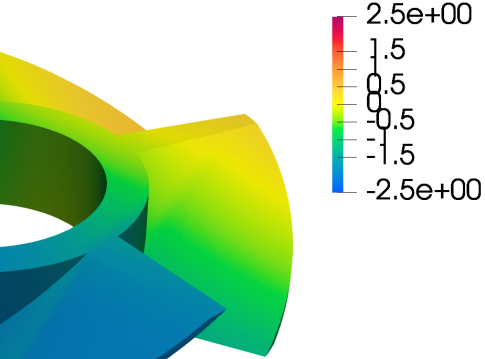
Figure 5. Sample realizations of the centered Gaussian process with $G^{3/2}$-asymptotically smooth covariance function taken for the numerical experiments.

To that end, we prescribe a reference Gaussian random field in terms of a Karhunen-Loéve expansion, i.e.,

$$\mathcal{Z}(\omega,x)=\sum_{k=0}^{\infty}\sqrt{\lambda_{k}}\varphi(\mathbf{x})Y_{k}(\omega),$$

with $Y_{k}\sim U([-1,1])$ and $\{(\lambda_{k},\varphi_{k})\}_{k=0}^{\infty}$ the eigenpairs of the integral operator

$$\mathcal{C}\colon L^{2}(\partial D)\to L^{2}(\partial D),\qquad(\mathcal{C}\varphi)(\mathbf{x})=\int_{\partial D}g_{\delta}(\mathbf{x},\mathbf{y})\varphi(\mathbf{y})\operatorname{d}\!\sigma(\mathbf{y}).$$

The covariance function $g_{\delta}$ is chosen as a modified Matérn-$9/2$ kernel

$$g_{\delta}(\mathbf{x},\mathbf{y})=\tilde{g}(\|\gamma_{\delta}(\mathbf{x})-\gamma_{\delta}(\mathbf{y})\|),\qquad\tilde{g}(r)=\bigg{(}1+3r+\frac{27r^{2}}{7}+\frac{18r^{3}}{7}+\frac{27r^{4}}{35}\bigg{)}e^{-3r},$$

where

$$\boldsymbol{\gamma}_{\delta}\colon\partial D\to\mathbb{R}^{3},\qquad\boldsymbol{\gamma}_{\delta}(x_{1},x_{2},x_{3}),=\begin{bmatrix}0.1+\Upsilon_{\delta}(2*x_{1}-1)x_{1}\\ x_{2}\\ x_{3}\end{bmatrix}$$

and

$$\Upsilon_{\delta}(t)=\frac{\upsilon_{\delta}(1-t)}{\upsilon_{\delta}(1-t)+\upsilon_{\delta}(t)},\qquad\upsilon_{\delta}(t)=\begin{cases}0,&t\leq 0,\\ e^{-t^{\frac{1}{1-\delta}}},&t>0,\end{cases}$$

is a partition of Gevrey class $\delta\geq 1$ with $\Upsilon(t)=1$ for $t<0$ and $\Upsilon(t)=0$ for $t>0$, see, e.g., [13]. For our numerical experiments we choose $\delta=3/2$, for which samples are illustrated in Figure 5. This makes the covariance function $g_{\delta}$ a $G^{3/2}$-asymptotically smooth kernel function.

The $\mathcal{H}^{2}$-implementation of the numerical experiments is based on the C++-Library Bembel [17], with compression parameters $\alpha=1$, $\beta=2$, $\eta=0.8$, and $n_{\min}=4$. We choose piecewise constant finite element spaces $V_{h_{\ell}}=W_{h_{\ell}}$, $\ell=0,1,2,\ldots$, on uniformly refined quadrilateral meshes with $C_{\text{uni}}=4$ and $h_{\ell}\sim 2^{-\ell}$, leading to dimensions of the finite element spaces and covariance matrices as in Table 1.

$L$	0	1	2	3	4	5	6
$\dim V_{h}=\dim W_{h}$	60	240	960	3 840	15 360	61 440	245 760
$\dim(W_{h}\otimes W_{h})$	3 600	57 600	921 600	$\approx 14.7\cdot 10^{6}$	$\approx 236\cdot 10^{6}$	$\approx 3.77\cdot 10^{9}$	$\approx 60.4\cdot 10^{9}$

Table 1. Dimensions of the used finite element spaces. The estimated covariance matrices are matrices in $\mathbb{R}^{\dim W_{h}\times\dim W_{h}}$, i.e., have $\dim(W_{h}\otimes W_{h})$ degrees of freedom.

The Gaussian random field samples $\Pi_{h_{\ell}}\mathcal{Z}$ are generated from a Karhunen Loéve expansion which is truncated at $10^{-3}h^{\ell}$ and computed from a pivoted Cholesky decomposition [30]. According to Corollary 4.10 and Theorem 5.5 it holds $\tilde{\gamma}=1$ and we can expect a linear convergence rate for our $\mathcal{H}^{2}$-MLSCE, if the sample numbers are chosen proportional to Theorem 5.5. For our particular example we choose the sample numbers listed in Table 2.

$L$	0	1	2	3	4	5	6
$M_{0}$	1	4	64	576	4 096	25 600	147 456
$M_{1}$		1	16	144	1 024	6 400	36 864
$M_{2}$			4	36	256	1 600	9 216
$M_{3}$				9	64	400	2 304
$M_{4}$					16	100	576
$M_{5}$						25	144
$M_{6}$							36

Table 2. Sample numbers chosen according to the case $2\tilde{\gamma}=d$ in Theorem 5.5 for the numerical example.

Figure 6 shows that we reach indeed the predicted rate convergence rate of Theorem 4.8 and a computational work vs. accuracy as in Theorem 5.5. The spectral error was computed with a power iteration up to an absolute accuracy of $10^{-4}$. The computation times are measured in wall clock time and have been carried out in parallel with 48 threads on a compute server with 1.3TB RAM and two Intel(R) Xeon(R) CPU E7-4850 v2 CPUs with Hyper-Threading enabled.

Figure 6. Convergence plot of a realization of the $\mathcal{H}^{2}$-MLSCE and corresponding computational work vs. accuracy with the sample numbers as in Table 2, cf. also Corollary 4.10 and Theorem 5.5.

7. Conclusion

In this article, we considered the multilevel estimation of covariance functions which are $G^{\delta}$-asymptotically smooth, $\delta\geq 1$. This choice is motivated by the stochastic partial differential equation approach to Gaussian random fields and pseudodifferential operator theory. The naive approach to estimate the covariance function from discretized samples using the single level covariance estimator is computationally prohibitive due to the density of the arising covariance matrices and the slow convergence of the sample covariance estimator. To overcome these issues, we first generalized the classical $\mathcal{H}^{2}$-approximation theory for asymptotically smooth kernels to Gevrey kernels. This allows to compress the arising covariance matrices by $\mathcal{H}^{2}$-matrices in linear complexity with respect to the underlying approximation space. Secondly, we proposed and analyzed an $\mathcal{H}^{2}$-formatted multilevel covariance sample estimator ($\mathcal{H}^{2}$-MLCSE). This estimator exploits an approximate multilevel hierarchy in the $\mathcal{H}^{2}$-approximation spaces to estimate the covariance in the same complexity as the mean. The provided approximation theory is applicable to a rather general setting, covering for example domains, manifolds, graphs, and multi-screens as well as various approximation spaces such as finite element spaces and Nyström discretizations.

Alternatively to the approach proposed in this paper, a wavelet based method for estimating covariance functions was proposed in [28]. The advantage of such a wavelet method is that the wavelet-based approximation results also hold for finite smoothness of the covariance function, whereas the here presented $\mathcal{H}^{2}$-approach requires asymptotically infinite smoothness. In contrast, the advantage of the $\mathcal{H}^{2}$-approach in this paper is that no wavelet basis is required and that the presented algorithms can be integrated into the many readily available $\mathcal{H}^{2}$-matrix codes.

Appendix A Computation of $\mathcal{H}^{2}$-related constants

Definition A.1 ([4, Definition 3.44]).

Let $T_{I}$ be a cluster tree and denote the number of interpolation points chosen in each cluster $t\in T_{I}$ by $K_{t}$. We say that $\{K_{t}\}_{t\in T_{I}}$ is a rank distribution. We say that $\{K_{t}\}_{t\in T_{I}}$ is a $(C_{bn},\alpha,\beta,r,\xi)$-bounded rank distribution, $C_{bn}\geq 1$, $\alpha>0$, $\beta\geq 0$, $r\geq 1$, $\xi\geq 1$, if

$$\big{|}\big{\{}t\in T_{I}\colon K_{t}>(\alpha+\beta(\ell-1))^{r}\big{\}}\big{|}\leq C_{bn}\xi^{-\ell}|T_{I}|,\qquad\text{for all}~{}\ell\in\mathbb{N}.$$

Lemma A.2.

Let $T_{I}$ be a cluster tree on the index set $I$ satisfying 2.12. Then $\{K_{t}\}_{t\in T_{I}}$ is a $(1,\alpha,\beta,\delta d,C_{\text{ab}})$-bounded rank distribution if the number of interpolation points in $(K_{t})_{t\in T_{I}}$ are chosen according to Equation 8, i.e.,

$$K_{t}=\big{\lceil}(\beta+\alpha(p-\operatorname{\operatorname{level}}(t)))^{\delta}\big{\rceil}^{d}$$

Proof.

The proof is analogy to the example in [4, p. 64]. Let $p$ denote the depth of $T_{I}$. We need to bound the number of clusters with

$$K_{t}=\big{\lceil}(\beta+\alpha(p-\operatorname{\operatorname{level}}(t)))^{\delta}\big{\rceil}^{d}\geq(\beta+\alpha(p-\operatorname{\operatorname{level}}(t)))^{\delta d}>(\alpha+\beta(\ell-1))^{\delta d}.$$

From this inequality we deduce that the clusters satisfying this constraint also satisfy $\operatorname{\operatorname{level}}(t)<p+1-\ell$. Due to 2.12 the number of such clusters is bounded by from above by $(C_{\text{ab}}^{p-\ell+2}-1)/(C_{\text{ab}}-1)$ and we obtain the assertion due to

$$|T_{I}|\geq\frac{C_{\text{ab}}^{p+2}-1}{C_{\text{ab}}-1}=C_{\text{ab}}^{\ell}\frac{C_{\text{ab}}^{p-\ell+2}-C_{\text{ab}}^{-\ell}}{C_{\text{ab}}-1}\geq C_{\text{ab}}^{\ell}\frac{C_{\text{ab}}^{p-\ell+2}-1}{C_{\text{ab}}-1}.$$

∎

Definition A.3 ([4, Definitions 3.43 and 3.47]).

Let $T_{I}$ be a cluster tree. We say that it is $(C_{rc},\alpha,\beta,r,\xi)$-bounded with $C_{rc}\geq 1$, $\alpha>0$, $\beta\geq 0$, $r\geq 1$, $\xi>1$, if

(22) $$\big{|}\big{\{}t\in L_{I}\colon|t|>(\beta+\alpha(\ell-1))^{r}\big{\}}\big{|}\leq C_{rc}\xi^{-\ell}|T_{I}|,\qquad\text{for all}~{}\ell\in\mathbb{N},$$

and

(23) $$|\operatorname{\operatorname{children}}(t)|\leq C_{rc},\qquad\text{for all}~{}t\in T_{I}.$$

We say that $T_{I}$ is $(C_{rc},\alpha,\beta,r,\xi)$-regular, if it is $(C_{rc},\alpha,\beta,r,\xi)$-bounded and additionally satisfies

(24) $$|\operatorname{\operatorname{children}}(t)| \geq 2, \text{for all}~{}t\in T_{I}\setminus L_{I},$$

(25) $$(\alpha+\beta)^{r} \leq C_{rc}|t|, \text{for all}~{}t\in L_{I}.$$

Lemma A.4.

Let $T_{I}$ be a cluster tree with depth $p$ on the index set $I$ satisfying 2.12. Then $T_{I}$ is $(C_{rc},\alpha,\beta,\delta d,C_{\text{ab}})$-regular with

(26) $$C_{\text{rc}}=\max\bigg{\{}C_{\text{ab}},\frac{(\alpha+\beta)^{\delta d}}{n_{\min}},C_{\text{ab}}^{\frac{n_{\min}^{1/(\delta d)}-\beta+\alpha}{\alpha}+1}\bigg{\}}.$$

Proof.

Equation 6 implies $2\leq|\operatorname{\operatorname{children}}(t)|\leq C_{\text{ab}}$, $t\in T_{I}\setminus L_{I}$, which yields (24) and Equation 23 holds with $C_{\text{rc}}\geq C_{\text{ab}}$. Inserting the upper bound from Equation 7 into Equation 25 yields

$$\frac{(\alpha+\beta)^{\delta d}}{n_{\min}}\leq C_{\text{rc}}.$$

Finally, the lower bound from Equation 7 implies that there are at most $C_{\text{ab}}^{p+1}$ leafs. The upper bound from Equation 7 and Equation 22 with $\xi=C_{\text{ab}}$ then imply that $C_{rc}$ must satisfy

$$C_{rc}\geq\begin{cases}\frac{C_{\text{ab}}^{p+\ell+1}}{|T_{I}|}&\text{for all}~{}\ell~{}\text{with}~{}(\beta+\alpha(\ell-1))^{\delta d}<n_{\min}\\ 0&\text{else}\end{cases}$$

Solving $(\beta+\alpha(\ell-1))^{\delta d}<n_{\min}$ for $\ell$ implies $\ell<(n_{\min}^{1/(\delta d)}-\beta+\alpha)/\alpha$ which yields

$$C_{\text{ab}}^{\frac{n_{\min}^{1/(\delta d)}-\beta+\alpha}{\alpha}+1}\leq C_{rc}$$

due to $|T_{I}|\geq(C_{\text{ab}}^{p+2}-1)/(C_{\text{ab}}-1)$. Combining all conditions on $C_{rc}$ yields the assertion. ∎

Lemma A.5 ([4, Lemma 3.45]).

Let $T_{I}$ be a $(C_{\text{rc}},\alpha,\beta,r,\xi)$-bounded cluster tree and let $\{K_{t}\}_{t\in T_{I}}$ be a $(C_{\text{bn}},\alpha,\beta,r,\xi)$-bounded rank distribution. Define

(27) $$k_{t}=\begin{cases}\max\{K_{t},|t|\},&t\in L_{I},\\ \max\{K_{t},\sum_{t^{\prime}\in\operatorname{\operatorname{children}}(t)}K_{t^{\prime}}\},&t\in T_{I}\setminus L_{I}.\end{cases}$$

and $m\in\mathbb{N}$. Then there is a constant $C_{\text{cb}}=C_{\text{cb}}(C_{\text{rc}},C_{\text{bn}},r,\xi)\geq 1$ such that

$$\sum_{t\in T_{I}}k_{t}^{m}\leq C_{\text{cb}}(\alpha+\beta)^{rm}|T_{I}|.$$

Lemma A.6 ([4, Lemma 3.48]).

Let $T_{I}$ be a $(C_{\text{rc}},\alpha,\beta,r,\xi)$-regular cluster tree. Then it holds

$$|T_{I}|\leq\frac{2C_{\text{rc}}|I|}{(\alpha+\beta)^{r}}$$

Lemma A.7 (Modification of [4, Corollary 3.49]).

Let $T_{I}$ be $(C_{\text{rc}},\alpha,\beta,r,\xi)$-bounded and $(K_{t})_{t\in T_{I}}$ be a $(C_{\text{bn}},\alpha,\beta,\xi)$-bounded rank distribution. Let $T_{I}$ be $(C_{\text{rc}},\alpha^{\prime},\beta^{\prime},r,\xi)$-regular and $T_{I\times I}$ be a block-cluster tree with sparsity constant $C_{\text{sp}}$. For $m\in\mathbb{N}$ and $\{k_{t}\}_{t\in T_{I}}$ defined as in Equation 27 it holds

$$\sum_{t\in T_{I}}k_{t}^{m}\leq C_{\mathcal{H}^{2}}\frac{(\alpha+\beta)^{rm}}{(\alpha^{\prime}+\beta^{\prime})^{r}}|I|$$

with $C_{\mathcal{H}^{2}}=2C_{\text{rc}}C_{\text{cb}}$.

Proof.

Combine Lemma A.5 and Lemma A.6. ∎

References

- [1] A. Barth, Ch. Schwab, and N. Zollinger. Multi-level Monte Carlo Finite Element method for elliptic PDEs with stochastic coefficients. Numerische Mathematik, 119(1):123–161, September 2011.
- [2] P. J. Bickel and E. Levina. Covariance regularization by thresholding. The Annals of Statistics, 36(6), December 2008.
- [3] P. J. Bickel and E. Levina. Regularized estimation of large covariance matrices. The Annals of Statistics, 36(1), February 2008.
- [4] S. Börm. Efficient Numerical Methods for Non-Local Operators, volume 14 of EMS Tracts in Mathematics. European Mathematical Society (EMS), Zürich, 2010.
- [5] S. Börm and J. Garcke. Approximating gaussian processes with -matrices. In Joost N. Kok, Jacek Koronacki, Raomon Lopez de Mantaras, Stan Matwin, Dunja Mladenič, and Andrzej Skowron, editors, Machine Learning: ECML 2007, pages 42–53, Berlin, Heidelberg, 2007. Springer Berlin Heidelberg.
- [6] S. Börm, M. Löhndorf, and J. M. Melenk. Approximation of Integral Operators by Variable-Order Interpolation. Numerische Mathematik, 99(4):605–643, February 2005.
- [7] Steffen Börm. On Iterated Interpolation. SIAM Journal on Numerical Analysis, 60(6):3124–3144, December 2022.
- [8] L. Boutet de Monvel and P. Krée. Pseudo-differential operators and Gevrey classes. Université de Grenoble. Annales de l’Institut Fourier, 17(fasc. 1):295–323, 1967.
- [9] S. C. Brenner and L. R. Scott. The Mathematical Theory of Finite Element Methods, volume 15 of Texts in Applied Mathematics. Springer New York, New York, NY, 2008.
- [10] H.-J. Bungartz and M. Griebel. Sparse grids. Acta Numerica, 13:147–269, May 2004.
- [11] T. T. Cai, Z. Ren, and H. H. Zhou. Estimating structured high-dimensional covariance and precision matrices: Optimal rates and adaptive estimation. Electronic Journal of Statistics, 10(1), January 2016.
- [12] J. E. Castrillón-Candás, M. G. Genton, and R. Yokota. Multi-level restricted maximum likelihood covariance estimation and kriging for large non-gridded spatial datasets. Spatial Statistics, 18:105–124, November 2016.
- [13] H. Chen and L. Rodino. General theory of PDE and Gevrey classes. In General theory of partial differential equations and microlocal analysis (Trieste, 1995), volume 349 of Pitman Res. Notes Math. Ser., pages 6–81. Longman, Harlow, 1996.
- [14] A. Chernov and Ch. Schwab. First order -th moment finite element analysis of nonlinear operator equations with stochastic data. Mathematics of Computation, 82(284):1859–1888, 2013.
- [15] M. Costabel, M. Dauge, and Ch. Schwab. Exponential convergence of hp-FEM for Maxwell equations with weighted regularization in polygonal domains. Mathematical Models and Methods in Applied Sciences, 15(04):575–622, April 2005.
- [16] J. Dick, F. Y. Kuo, and I. H. Sloan. High-dimensional integration: The quasi-Monte Carlo way. Acta Numerica, 22:133–288, 2013.
- [17] J. Dölz, H. Harbrecht, S. Kurz, M. Multerer, S. Schöps, and F. Wolf. Bembel: The fast isogeometric boundary element C++ library for Laplace, Helmholtz, and electric wave equation. SoftwareX, 11:100476, January 2020.
- [18] J. Dölz, H. Harbrecht, and Ch. Schwab. Covariance regularity and -matrix approximation for rough random fields. Numerische Mathematik, 135(4):1045–1071, 2017.
- [19] N. El Karoui. Operator norm consistent estimation of large-dimensional sparse covariance matrices. The Annals of Statistics, 36(6), December 2008.
- [20] J. Fan, Y. Liao, and H. Liu. An overview of the estimation of large covariance and precision matrices. The Econometrics Journal, 19(1):C1–C32, February 2016.
- [21] R. Furrer, Marc G. Genton, and D. Nychka. Covariance Tapering for Interpolation of Large Spatial Datasets. Journal of Computational and Graphical Statistics, 15(3):502–523, September 2006.
- [22] A. Garriga-Alonso, L. Aitchison, and C. E. Rasmussen. Deep Convolutional Networks as shallow Gaussian Processes. In 7th International Conference on Learning Representations, May 2019.
- [23] R. Ghanem, D. Higdon, and H. Owhadi, editors. Handbook of Uncertainty Quantification. Springer International Publishing, Cham, 2017.
- [24] M. B. Giles. Multilevel Monte Carlo methods. Acta Numerica, 24:259, 2015.
- [25] L. Greengard and V. Rokhlin. A fast algorithm for particle simulations. Journal of Computational Physics, 73(2):325–348, December 1987.
- [26] W. Hackbusch. Integral Equations, volume 120 of International Series of Numerical Mathematics. Birkhäuser, Basel, 1995.
- [27] W. Hackbusch. Hierarchical Matrices: Algorithms and Analysis. Springer, Heidelberg, 2015.
- [28] H. Harbrecht, L. Herrmann, K. Kirchner, and Ch. Schwab. Multilevel approximation of Gaussian random fields: Covariance compression, estimation and spatial prediction. Technical Report 2021-09, Seminar for Applied Mathematics, ETH Zürich, Switzerland, 2021.
- [29] H. Harbrecht and M. Multerer. Samplets: Construction and scattered data compression. Journal of Computational Physics, 471:111616, December 2022.
- [30] H. Harbrecht, M. Peters, and M. Siebenmorgen. Efficient approximation of random fields for numerical applications. Numerical Linear Algebra with Applications, 22(4):596–617, 2015.
- [31] S. Heinrich. Multilevel Monte Carlo Methods. In S. Margenov, J. Waśniewski, and P. Yalamov, editors, Large-Scale Scientific Computing, volume 2179, pages 58–67. Springer Berlin Heidelberg, Berlin, Heidelberg, 2001.
- [32] L. Herrmann, K. Kirchner, and Ch. Schwab. Multilevel approximation of Gaussian random fields: Fast simulation. Mathematical Models and Methods in Applied Sciences, 30(01):181–223, January 2020.
- [33] T. Hofmann, B. Schölkopf, and A. J. Smola. Kernel methods in machine learning. The Annals of Statistics, 36(3), June 2008.
- [34] R. A. Johnson and D. W. Wichern. Applied Multivariate Statistical Analysis. Pearson Prentice Hall, Upper Saddle River, N.J, 6th ed edition, 2007.
- [35] B. N. Khoromskij, A. Litvinenko, and H. G. Matthies. Application of hierarchical matrices for computing the Karhunen–Loève expansion. Computing, 84(1-2):49–67, April 2009.
- [36] D. Kressner, J. Latz, S. Massei, and E. Ullmann. Certified and fast computations with shallow covariance kernels. Foundations of Data Science, 2(4):487–512, 2020.
- [37] F. Y. Kuo, Ch. Schwab, and I. H. Sloan. Multi-level Quasi-Monte Carlo Finite Element Methods for a class of elliptic PDEs with random coefficients. Foundations of Computational Mathematics, 15(2):411–449, April 2015.
- [38] F. Lindgren, H. Rue, and J. Lindström. An explicit link between Gaussian fields and Gaussian Markov random fields: The stochastic partial differential equation approach: Link between Gaussian Fields and Gaussian Markov Random Fields. Journal of the Royal Statistical Society: Series B (Statistical Methodology), 73(4):423–498, September 2011.
- [39] A. Litvinenko, Y. Sun, Y. G. Genton, and D. E. Keyes. Likelihood approximation with hierarchical matrices for large spatial datasets. Computational Statistics & Data Analysis, 137:115–132, September 2019.
- [40] B. Matérn. Spatial Variation. Meddelanden frn Statens Skogsforskningsinstitut, 49(5), 1960.
- [41] V. Minden, A. Damle, K. L. Ho, and L. Ying. Fast Spatial Gaussian Process Maximum Likelihood Estimation via Skeletonization Factorizations. Multiscale Modeling & Simulation, 15(4):1584–1611, January 2017.
- [42] P. Mycek and M. De Lozzo. Multilevel Monte Carlo Covariance Estimation for the Computation of Sobol’ Indices. SIAM/ASA Journal on Uncertainty Quantification, 7(4):1323–1348, January 2019.
- [43] J. A. A. Opschoor, Ch. Schwab, and J. Zech. Exponential ReLU DNN expression of holomorphic maps in high dimension. Constructive Approximation, 55(1):537–582, February 2022.
- [44] C. E. Rasmussen and Ch. K. I. Williams. Gaussian Processes for Machine Learning. Adaptive Computation and Machine Learning. MIT Press, Cambridge, Mass, 2006.
- [45] T. J. Rivlin. The Chebyshev Polynomials. Pure and Applied Mathematics. Wiley, New York, 1974.
- [46] F. Schäfer, T. J. Sullivan, and H. Owhadi. Compression, Inversion, and Approximate PCA of Dense Kernel Matrices at Near-Linear Computational Complexity. Multiscale Modeling & Simulation, 19(2):688–730, January 2021.
- [47] R. Schneider. Multiskalen- Und Wavelet-Matrixkompression. Advances in Numerical Mathematics. Vieweg+Teubner Verlag, Wiesbaden, 1998.
- [48] Ch. Schwab and R. A. Todor. Karhunen-Loève approximation of random fields by generalized fast multipole methods. Journal of Computational Physics, 217(1):100–122, 2006.
- [49] M. L. Stein. Interpolation of Spatial Data: Some Theory for Kriging. Springer, New York, 2013.
- [50] H. Wendland. Scattered Data Approximation. Cambridge University Press, first edition, December 2004.
- [51] P. Whittle. Stochastic processes in several dimensions. Bulletin de l’Institut International de Statistique, 40:974–994, 1963.