Reduced-Order Autodifferentiable Ensemble Kalman Filters

Abstract

This paper introduces a computational framework to reconstruct and forecast a partially observed state that evolves according to an unknown or expensive-to-simulate dynamical system. Our reduced-order autodifferentiable ensemble Kalman filters (ROAD-EnKFs) learn a latent low-dimensional surrogate model for the dynamics and a decoder that maps from the latent space to the state space. The learned dynamics and decoder are then used within an ensemble Kalman filter to reconstruct and forecast the state. Numerical experiments show that if the state dynamics exhibit a hidden low-dimensional structure, ROAD-EnKFs achieve higher accuracy at lower computational cost compared to existing methods. If such structure is not expressed in the latent state dynamics, ROAD-EnKFs achieve similar accuracy at lower cost, making them a promising approach for surrogate state reconstruction and forecasting.

1 Introduction

Reconstructing and forecasting a time-evolving state given partial and noisy time-series data is a fundamental problem in science and engineering, with far-ranging applications in numerical weather forecasting, climate, econometrics, signal processing, stochastic control, and beyond. Two common challenges are the presence of model error in the dynamics governing the evolution of the state, and the high computational cost to simulate operational model dynamics. Model error hinders the accuracy of forecasts, while the computational cost to simulate the dynamics hinders the quantification of uncertainties in these forecasts. Both challenges can be alleviated by leveraging data to learn a surrogate model for the dynamics. Data-driven methods enable learning closure terms and unresolved scales in the dynamics, thus enhancing the forecast skill of existing models. In addition, surrogate models are inexpensive to simulate and enable using a large number of particles within ensemble Kalman or Monte Carlo methods for state reconstruction and forecasting, thus enhancing the uncertainty quantification.

This paper investigates a framework for state reconstruction and forecasting that relies on data-driven surrogate modeling of the dynamics in a low-dimensional latent space. Our reduced-order autodifferentiable ensemble Kalman filters (ROAD-EnKFs) leverage the EnKF algorithm to estimate by maximum likelihood the latent dynamics as well as a decoder from latent space to state space. The learned latent dynamics and decoder are subsequently used to reconstruct and forecast the state. Numerical experiments show that, compared to existing methods, ROAD-EnKFs achieve higher accuracy at lower computational cost provided that the state dynamics exhibit a hidden low-dimensional structure. When such structure is not expressed in the latent dynamics, ROAD-EnKFs achieve similar accuracy at lower cost, making them a promising approach for surrogate state reconstruction and forecasting.

Our work blends in an original way several techniques and insights from inverse problems, data assimilation, machine learning, and reduced-order modeling. First, if the state dynamics were known and inexpensive to simulate, a variety of filtering and smoothing algorithms from data assimilation (e.g. extended, ensemble, and unscented Kalman filters and smoothers, as well as particle filters) can be used to reconstruct and forecast the state. These algorithms often build on a Bayesian formulation, where posterior inference on the state combines the observed data with a prior distribution defined using the model dynamics. Hence, learning a surrogate model for the dynamics can be interpreted as learning a prior regularization for state reconstruction and forecasting. Second, the task of learning the regularization can be viewed as an inverse problem: we seek to recover the state dynamics from partially and noisily observed trajectories. Data assimilation facilitates the numerical solution of this inverse problem by providing estimates of the hidden state. Third, our work leverages machine learning and reduced-order modeling to parameterize the dynamics in a low-dimensional latent space and learn a decoder from latent space to state space. In particular, we parameterize the decoder using recent ideas from discretization-invariant operator learning. Our numerical experiments demonstrate the computational advantage of co-learning an inexpensive surrogate model in latent space together with a decoder, rather than a more expensive-to-simulate dynamics in state space.

1.1 Related Work

Ensemble Kalman Filters in Data Assimilation

The EnKF algorithm, reviewed in [44, 47, 72, 75], is a popular method for state reconstruction and forecasting in data assimilation, with applications in numerical weather forecasting, the geophysical sciences, and signal processing [29, 30, 83, 91]. The EnKF propagates $N$ equally-weighted particles through the dynamics, and assimilates new observations via Kalman-type updates computed with empirical moments. If the state dynamics are known, the EnKF can achieve accurate reconstruction with a small ensemble size $N$ even in applications where the state and the observations are high-dimensional, provided that the effective dimension is moderate [32]; EnKFs with a small ensemble size have a low computational and memory cost compared to traditional Kalman filters [72]. Ensemble Kalman methods are also successful solvers for inverse problems, as reviewed in [14]. In this paper, we employ the EnKF to approximate the data log-likelihood of surrogate models for unknown or expensive-to-simulate dynamics. The use of the EnKF for maximum likelihood estimation (MLE) was first proposed in [81], which adopted a derivative-free optimization approach; see also [70]. Empirical studies on the likelihood computed with EnKFs and other data assimilation techniques can be found in [12, 64]. The application of the EnKF to approximate the data log-likelihood within pseudo-marginal Markov chain Monte Carlo methods for Bayesian parameter estimation was investigated in [28]; see also [79, 80]. The paper [20] introduced derivative-based optimization of an EnKF approximation of the log-likelihood to perform state and parameter estimation in high-dimensional nonlinear systems. However, to the best of our knowledge, no prior work combines estimation of the log-likelihood via EnKFs with learning low-dimensional surrogate models, including both surrogate latent dynamics and a decoder from latent space to state space.

Blending Data Assimilation with Reduced-Order Models

Model reduction techniques have been employed in data assimilation to improve the state reconstruction accuracy in high-dimensional dynamical systems. The assimilation in the unstable subspace (AUS) method [13, 87, 67, 74, 51] projects the dynamics onto a time-dependent subspace of the tangent space where the dynamics are unstable, and assimilates the observations therein. The unstable directions are determined by the Lyapunov vectors with nonnegative Lyapunov exponents, and can be approximated using discrete QR algorithms [24, 25]. The observations can also be projected onto the unstable directions to reduce the data dimension [59]. We refer to [5] for a review of projection-based model reduction techniques. However, these methods rely on prior knowledge about the dynamics to identify the unstable subspaces and to construct the latent dynamics, and data assimilation is performed after the subspaces are found. In contrast, our paper introduces a framework that uses data assimilation as a tool to build surrogate latent dynamics from data. Another approach to reduce the dimension of data assimilation problems exploits the conditionally Gaussian distribution of slow variables arising in the stochastic parameterization of a wide range of dynamical systems [18, 17, 61]. This conditional Gaussian structure can be exploited to obtain adequate uncertainty quantification of forecasts with a moderate sample size. A caveat, however, is that identifying the slow variables can be challenging in practice. As in our approach, these techniques often rely on machine learning to learn closure terms for the dynamics [18]. Finally, we refer to [78] for a discussion on how the effective dimension of transport map methods for data assimilation can be reduced by exploiting the conditional independence structure of the reference-target pair.

Merging Data Assimilation with Machine Learning

Recent developments in machine learning to model dynamical systems from data are reviewed in [55]. One line of work [84, 88, 27, 70] embeds the EnKF and the ensemble Kalman smoother (EnKS) into the expectation-maximization (EM) algorithm for MLE [23], with a special focus on estimation of error covariance matrices. The expectation step (E-step) is approximated by EnKF/EnKS with the Monte Carlo EM objective [90]. A subsequent line of work [66, 9, 7, 31, 92] introduces training of a neural network (NN) surrogate model in the maximization step (M-step) based on the states filtered by the E-step. Unfortunately, it can be hard to achieve an accurate approximation of the E-step using EnKF/EnKS [20]. Another line of work [65, 60, 52, 21] approximates the data log-likelihood with particle filters (PFs) [35, 26] and performs MLE using derivative-based optimization. However, the resampling step in PFs is not readily differentiable, and, in addition, PFs often collapse when the dimensions of the state and the observations are large [2, 4]. Finally, techniques that leverage machine learning to obtain inexpensive analog ensembles for data assimilation are starting to emerge [95].

Data-Driven Modeling of Dynamical Systems with Machine Learning

Machine learning is also useful for dimensionality reduction in time-series modeling. As an important example, recurrent neural networks (RNNs) [57, 96] assimilate data into the time-evolving latent states using NN updates. The paper [73] models the latent state evolution in recurrent networks with NN-embedded differential equations [19]. Other types of NN updates to incorporate the data into latent states include gated recurrent units (GRU) [22, 45], long short-term memory (LSTM) [54, 39], and controlled differential equations (CDEs) [48]. Another approach is to directly model the differential equation governing the state dynamics from observation data using regression. Such methods include sparse regression over a dictionary of candidate functions using $L_{1}$-regularization [10, 86, 76]. These techniques rely on full observation of the state, and, importantly, on time-derivative data that are rarely available in practice and are challenging to approximate from noisy discrete-time observation data [41, 40]. When the data are not guaranteed to lie in the same space as the underlying dynamics, an autoencoder structure can be jointly learned with the latent state dynamics [16]. Different modeling techniques can be applied to learn the latent state dynamics, including sparse dictionary regression [16], recurrent networks [34, 63], and the Koopman operator learning [58]. It is important to notice that, in contrast to, e.g., [10, 42], the focus of this paper is on state reconstruction and forecasting, rather than on obtaining an interpretable model for the dynamics.

1.2 Outline and Main Contributions

• Section 2 formalizes the problem setting and goals. We introduce a reduced-order state-space model (SSM) framework, where the dynamics are modeled in a low-dimensional latent space and learned jointly with a decoder from latent space to state space.

• Section 3 introduces our main algorithm, the reduced-order autodifferentiable ensemble Kalman filter (ROAD-EnKF). As part of the derivation of the algorithm, we discuss the use of EnKFs to estimate the data log-likelihood within reduced-order SSMs.

• Section 4 contains important implementation considerations, including the design of the decoder, the use of truncated backpropagation to enhance the scalability for large windows of data, and the choice of regularization in latent space.

• Section 5 demonstrates the performance of our method in three examples: (i) a Lorenz 63 model embedded in a high-dimensional space, where we compare our approach to the SINDy-AE algorithm [16]; (ii) Burgers equation, where we showcase that ROAD-EnKFs are able to forecast the emergence of shocks, a phenomenon not included in our training data-set; and (iii) Kuramoto-Sivashinky equation, a common test problem for filtering methods due to its chaotic behavior, where the ROAD-EnKF framework provides a computational benefit over state-of-the-art methods with similar accuracies.

• Section 6 closes with a summary of the paper and open questions for further research.

Notation

We denote by $t\in\{0,1,\dots\}$ a discrete-time index and by $n\in\{1,\dots,N\}$ a particle index. Time indices will be denoted with subscripts and particles with superscripts, so that $u_{t}^{n}$ represents a generic particle $n$ at time $t.$ We denote the particle dimension by $d_{u}.$ We denote $u_{t_{0}:t_{1}}:=\{u_{t}\}_{t=t_{0}}^{t_{1}}$ and $u^{n_{1}:n_{2}}:=\{u^{n}\}_{n=n_{0}}^{n_{1}}$. The collection $u_{t_{0}:t_{1}}^{n_{0}:n_{1}}$ is defined similarly. The Gaussian density with mean $m$ and covariance $C$ evaluated at $u$ is denoted by $\mathcal{N}(u;m,C)$. The corresponding Gaussian distribution is denoted by $\mathcal{N}(m,C)$.

2 Problem Formulation

In this section, we formalize and motivate our goals: reconstructing and forecasting a time-evolving, partially-observed state with unknown or expensive-to-simulate dynamics. An important step towards these goals is to learn a surrogate model for the dynamics. In Subsection 2.1 we consider an SSM framework where the state dynamics are parameterized and learned in order to reconstruct and forecast the state. Next, in Subsection 2.2, we introduce a reduced-order SSM framework where the dynamics are modeled in a latent space and a decoder from latent space to state space is learned along with the latent dynamics. Our ROAD-EnKF algorithm, introduced in Section 3, operates in this reduced-order SSM.

2.1 Setting and Motivation

Consider a parameterized SSM of the form:

(dynamics) $$\quad\quad u_{t} =F_{\alpha}(u_{t-1})+\xi_{t},\quad\quad \xi_{t}\sim\mathcal{N}(0,Q_{\beta}),\quad\quad 1\leq t\leq T,$$ (2.1)

(observation) $$\quad\quad y_{t} =H_{t}u_{t}+\eta_{t},\quad\quad \eta_{t}\sim\mathcal{N}(0,R_{t}),\quad\quad 1\leq t\leq T,$$ (2.2)

(initialization) $$\quad\quad u_{0} \sim p_{u}(u_{0}).$$ (2.3)

The state dynamics map $F_{\alpha}:\mathbbm{R}^{d_{u}}\rightarrow\mathbbm{R}^{d_{u}}$ and error covariance matrix $Q_{\beta}\in\mathbbm{R}^{d_{u}\times d_{u}}$ depend on unknown parameter $\theta:=(\alpha^{\top},\beta^{\top})^{\top}\in\mathbbm{R}^{d_{\theta}}$. The observation matrices $H_{t}\in\mathbbm{R}^{d_{y}\times d_{u}}$ and error covariance matrices $R_{t}\in\mathbbm{R}^{d_{y}\times d_{y}}$ are assumed to be known and possibly time-varying. We further assume independence of all random variables $u_{0}$, $\xi_{1:T},$ and $\eta_{1:T}$.

Given observation data $y_{1:T}$ drawn from the SSM (2.1)-(2.3), we aim to accomplish two goals:

1. Reconstruct the states $u_{1:T}$.

2. Forecast the states $u_{T+1:T+T_{f}}$ for some forecast lead time $T_{f}\geq 1$.

Figure 1: Structure of data under SSM (2.1)-(2.3), where we assume only observations $y_{1:T}:=\{y_{1},\dots,y_{T}\}$ are available. Our goals are to reconstruct the states $u_{1:T}$ (Goal 1) and to forecast future states $u_{T+1:T+T_{f}}$ for some $T_{f}\geq 1$ (Goal 2).

If the true parameter $\theta\in\mathbbm{R}^{d_{\theta}}$ was known and the dynamics were inexpensive to simulate, the first goal can be accomplished by applying a filtering (or smoothing) algorithm on the SSM (2.1)-(2.3), while the second goal can be accomplished by iteratively applying the dynamics model 2.1 to the reconstructed state $u_{T}$. We are interested in the case where $\theta$ needs to be estimated in order to reconstruct and forecast the state.

The covariance $Q_{\beta}$ in the dynamics model (2.1) may represent model error or stochastic forcing in the dynamics; in either case, estimating $Q_{\beta}$ from data can improve the reconstruction and forecast of the state. In this paper, we are motivated by applications where $F_{\alpha}$ represents a surrogate model for the flow between observations of an autonomous ordinary differential equation (ODE). Letting $\Delta_{s}$ be the equally-spaced time between observations and $f_{\alpha}:\mathbbm{R}^{d_{u}}\mapsto\mathbbm{R}^{d_{u}}$ be the parameterized vector field of the differential equation, we then have

$$\text{(ODE)}\quad\quad\frac{\text{d}u}{\text{d}s}=f_{\alpha}(u),\quad\quad F_{\alpha}:u(s)\mapsto u(s+\Delta_{s}),$$ (2.4)

where $u(s)\in\mathbbm{R}^{d_{u}}$ is the state as a function of continuous-time variable $s\geq 0$. The ODE (2.4) may arise from spatial discretization of a system of partial differential equations (PDEs). For instance, we will consider 1-dimensional partial differential equations for $u(x,s)$ of order $\kappa\geq 1,$ where $u$ is a function of the spatial variable $x\in[0,\mathsf{L}]$ and continuous-time variable $s\geq 0$:

$$\text{(PDE)}\quad\quad\frac{\partial u}{\partial s}=f_{\alpha}\biggl{(}u,\frac{\partial u}{\partial x},\dots,\frac{\partial^{\kappa}u}{\partial x^{\kappa}}\biggr{)},\quad\quad F_{\alpha}:u(\cdot,s)\mapsto u(\cdot,s+\Delta_{s}),$$ (2.5)

with suitable boundary conditions. After discretizing this equation on a spatial domain with grid points $0=x_{1}<x_{2}<\cdots<x_{M}=\mathsf{L}$, 2.5 can be expressed in the form of 2.4 by replacing the spatial derivatives with their finite difference approximations, and $u,f_{\alpha},F_{\alpha}$ with their finite-dimensional approximations on the grid. As a result, $d_{u}$ equals the number of grid points $M$. Several examples and additional details will be given in Section 5.

2.2 Reduced-Order Modeling

When the state is high-dimensional (i.e., $d_{u}$ is large), direct reconstruction and forecast of the state is computationally expensive, and surrogate modeling of the state dynamics map $F_{\alpha}$ becomes challenging. We then advocate reconstructing and forecasting the state $u_{t}$ through a low-dimensional latent representation $z_{t}$, modeling the state dynamics within the low-dimensional latent space. This idea is formalized via the following reduced-order parameterized SSM:

(latent dynamics) $$\quad\quad z_{t} =G_{\alpha}(z_{t-1})+\zeta_{t},\quad\quad \zeta_{t}\sim\mathcal{N}(0,S_{\beta}),\quad\quad 1\leq t\leq T,$$ (2.6)

(decoding) $$\quad\quad u_{t} =D_{\gamma}(z_{t}),\quad\quad 1\leq t\leq T,$$ (2.7)

(observation) $$\quad\quad y_{t} =H_{t}u_{t}+\eta_{t},\quad\quad \eta_{t}\sim\mathcal{N}(0,R_{t}),\quad\quad 1\leq t\leq T,$$ (2.8)

(latent initialization) $$\quad\quad z_{0} \sim p_{z}(z_{0}).$$ (2.9)

The latent dynamics map $G_{\alpha}:\mathbbm{R}^{d_{z}}\mapsto\mathbbm{R}^{d_{z}}$ and error covariance matrix $S_{\beta}\in\mathbbm{R}^{d_{z}\times d_{z}}$ are defined on a $d_{z}$ dimensional latent space with $d_{z}<d_{u}$, and the decoder function $D_{\gamma}:\mathbbm{R}^{d_{z}}\mapsto\mathbbm{R}^{d_{u}}$ maps from latent space to state space. The reduced-order SSM depends on an unknown parameter $\theta:=(\alpha^{\top},\beta^{\top},\gamma^{\top})^{\top}\in\mathbbm{R}^{d_{\theta}}$. The remaining assumptions are the same as in Subsection 2.1.

Figure 2: Structure of data under reduced-order SSM (2.6)-(2.9), where we assume only observations $y_{1:T}:=\{y_{1},\dots,y_{T}\}$ are available. Our goals are to reconstruct the states $u_{1:T}$ (Goal 1) and to forecast future states $u_{T+1:T+T_{f}}$ for some $T_{f}\geq 1$ (Goal 2).

Writing $\mathcal{H}_{\gamma,t}(\cdot):=H_{t}D_{\gamma}(\cdot)$, the reduced-order SSM (2.6)-(2.9) can be combined into

(latent dynamics) $$\quad\quad z_{t} =G_{\alpha}(z_{t-1})+\zeta_{t},\quad\quad \zeta_{t}\sim\mathcal{N}(0,S_{\beta}),\quad\quad 1\leq t\leq T,$$ (2.10)

(observation) $$\quad\quad y_{t} =\mathcal{H}_{\gamma,t}(z_{t})+\eta_{t},\quad\quad \eta_{t}\sim\mathcal{N}(0,R_{t}),\quad\quad 1\leq t\leq T,$$ (2.11)

(latent initialization) $$\quad\quad z_{0} \sim p(z_{0}),$$ (2.12)

where the observation function $\mathcal{H}_{\gamma,t}(\cdot)$ is nonlinear if the decoder $D_{\gamma}(\cdot)$ is nonlinear. As in Subsection 2.1, the map $G_{\alpha}$ may be interpreted as the flow between observations of an ODE with vector field $g_{\alpha}:\mathbbm{R}^{d_{z}}\mapsto\mathbbm{R}^{d_{z}}.$

If the true parameter $\theta\in\mathbbm{R}^{d_{\theta}}$ was known, given observation data $y_{1:T}$ drawn from the reduced-order SSM (2.6)-(2.9), we can reconstruct the states $u_{1:T}$ (Goal 1) by first applying a filtering (or smoothing) algorithm on (2.10)-(2.12) to estimate $z_{1:T}$, and then applying the decoder $D_{\gamma}$. We can forecast the states $u_{T+1:T+T_{f}}$ (Goal 2) by first applying iteratively the latent dynamics model 2.6 to the reconstructed latent state $z_{T}$, and then applying the decoder $D_{\gamma}$. As in Subsection 2.1, we are interested in the case where $\theta$ needs to be estimated from the given data $y_{1:T}$.

3 Reduced-Order Autodifferentiable Ensemble Kalman Filters

As discussed in the previous section, to achieve both goals of state reconstruction and forecast, it is essential to obtain a suitable surrogate model for the dynamics by learning the parameter $\theta$. The general approach we take is the following: (1) estimate $\theta$ with maximum likelihood; (2) apply a filtering algorithm with estimated parameter $\theta$ to reconstruct and forecast the states $u_{1:T}$. As we shall see, the maximum likelihood estimation of $\theta$ will rely itself on a filtering algorithm. For the SSM in Subsection 2.1, this approach was introduced in [20] via AD-EnKF (Algorithm 4.1 in [20]). Here we focus on the reduced-order SSM in Subsection 2.2, namely (2.10)-(2.12), which is a more general case than the SSM in Subsection 2.1; this explains the terminology reduced-order AD-EnKF (ROAD-EnKF).

In Subsection 3.1, we describe how the log-likelihood $\mathcal{L}(\theta)=\log p_{\theta}(y_{1:T})$ can be expressed in terms of the normalizing constants that arise from sequential filtering. In Subsection 3.2, we give background on EnKFs and on how to use these filtering algorithms to estimate $\mathcal{L}(\theta)$. In Subsection 3.3, we introduce our ROAD-EnKF method that takes as input multiple independent instances of observation data $y_{1:T}^{\mathcal{I}}$ across the same time range, and performs both state reconstruction and forecasting.

3.1 Sequential Filtering and Data Log-Likelihood

Suppose that $\theta=(\alpha^{\top},\beta^{\top},\gamma^{\top})^{\top}$ is known. We recall that, for $1\leq t\leq T,$ the filtering distributions $p_{\theta}(z_{t}|y_{1:t})$ of the SSM (2.10)-(2.12) can be obtained sequentially, alternating between prediction and analysis steps:

(prediction) $$\quad\quad p_{\theta}(z_{t}|y_{1:t-1})=\int\mathcal{N}\big{(}z_{t};G_{\alpha}(z_{t-1}),S_{\beta}\big{)}p_{\theta}(z_{t-1}|y_{1:t-1})\,\text{d}z_{t-1},$$ (3.1)

(analysis) $$\quad\quad p_{\theta}(z_{t}|y_{1:t})=\frac{1}{\mathcal{E}_{t}(\theta)}\mathcal{N}\big{(}y_{t};\mathcal{H}_{\gamma,t}(z_{t}),R_{t}\big{)}p_{\theta}(z_{t}|y_{1:t-1}),$$ (3.2)

with the convention $p_{\theta}(\cdot|y_{1:0}):=p_{\theta}(\cdot)$. Here $\mathcal{E}_{t}(\theta)$ is a normalizing constant which does not depend on $z_{t}$. It can be shown that

$$\mathcal{E}_{t}(\theta)=p_{\theta}(y_{t}|y_{1:t-1})=\int\mathcal{N}\big{(}y_{t};\mathcal{H}_{\gamma,t}(z_{t}),R_{t}\big{)}p_{\theta}(z_{t}|y_{1:t-1})\,\text{d}z_{t},$$ (3.3)

and therefore the data log-likelihood admits the characterization

$$\mathcal{L}(\theta):=\log p_{\theta}(y_{1:T})=\sum_{t=1}^{T}\log p_{\theta}(y_{t}|y_{1:t-1})=\sum_{t=1}^{T}\log\mathcal{E}_{t}(\theta).$$ (3.4)

Analytical expressions of the filtering distributions $p_{\theta}(z_{t}|y_{1:t})$ and the data log-likelihood $\mathcal{L}(\theta)$ are only available for a small class of SSMs, which includes linear-Gaussian and discrete SSMs [46, 68]. Outside these special cases, filtering algorithms need to be employed to approximate the filtering distributions, and these algorithms can be leveraged to estimate the log-likelihood.

3.2 Estimation of the Log-Likelihood with Ensemble Kalman Filters

Given $\theta=(\alpha^{\top},\beta^{\top},\gamma^{\top})^{\top}$, the EnKF algorithm [29, 30] sequentially approximates the filtering distributions $p_{\theta}(z_{t}|y_{1:t})$ using $N$ equally-weighted particles ${z}_{t}^{1:N}.$ At prediction steps, each particle ${z}_{t}^{n}$ is propagated using the latent dynamics model 2.10, while at analysis steps a Kalman-type update is performed for each particle:

(prediction step) $$\quad\quad\widehat{z}_{t}^{\,n}=G_{\alpha}({z}_{t-1}^{n})+{\zeta}_{t}^{n}, \quad\quad{\zeta}_{t}^{n}\overset{\text{i.i.d.}}{\sim}\mathcal{N}(0,S_{\beta}),$$ (3.5)

(analysis step) $$\quad\quad{z}_{t}^{n}=\widehat{z}_{t}^{\,n}+\widehat{K}_{t}\bigl{(}y_{t}+{\eta}_{t}^{n}-\mathcal{H}_{\gamma,t}(\widehat{z}_{t}^{\,n})\bigr{)}, \quad\quad{\eta}_{t}^{n}\overset{\text{i.i.d.}}{\sim}\mathcal{N}(0,R_{t}).$$ (3.6)

The Kalman gain $\widehat{K}_{t}:=\widehat{C}_{zy,t}(\widehat{C}_{yy,t}+R_{t})^{-1}$ is defined using empirical covariances given by

$$\widehat{C}_{zy,t}=\frac{1}{N-1}\sum_{n=1}^{N}(\widehat{z}_{t}^{\,n}-\widehat{m}_{t})\big{(}\mathcal{H}_{\gamma,t}(\widehat{z}_{t}^{\,n})-\widehat{\mathcal{H}}_{t}\big{)}^{\top},\quad\widehat{C}_{yy,t}=\frac{1}{N-1}\sum_{n=1}^{N}\big{(}\mathcal{H}_{\gamma,t}(\widehat{z}_{t}^{\,n})-\widehat{\mathcal{H}}_{t}\big{)}\big{(}\mathcal{H}_{\gamma,t}(\widehat{z}_{t}^{\,n})-\widehat{\mathcal{H}}_{t}\big{)}^{\top},$$ (3.7)

where

$$\widehat{m}_{t}=\frac{1}{N}\sum_{n=1}^{N}\widehat{z}_{t}^{\,n},\quad\quad\widehat{\mathcal{H}}_{t}=\frac{1}{N}\sum_{n=1}^{N}\mathcal{H}_{\gamma,t}(\widehat{z}_{t}^{\,n}).$$ (3.8)

The empirical moments $\widehat{C}_{yy,t},\widehat{\mathcal{H}}_{t}$ defined in equations 3.7 and 3.8 provide a Gaussian approximation to the predictive distribution for $\mathcal{H}_{\gamma,t}(z_{t})$:

$$p_{\theta}(\mathcal{H}_{\gamma,t}(z_{t})|y_{1:t-1})\approx\mathcal{N}(\mathcal{H}_{\gamma,t}(z_{t});\widehat{\mathcal{H}}_{t},\widehat{C}_{yy,t}).$$ (3.9)

By applying the change of variables formula to 3.3, we have

$$\begin{split}\mathcal{E}_{t}(\theta)&=\int\mathcal{N}\big{(}y_{t};\mathcal{H}_{\gamma,t}(z_{t}),R_{t}\big{)}p_{\theta}(z_{t}|y_{1:t-1})\,\text{d}z_{t}\\ &=\int\mathcal{N}\big{(}y_{t};\mathcal{H}_{\gamma,t}(z_{t}),R_{t}\big{)}p_{\theta}(\mathcal{H}_{\gamma,t}(z_{t})|y_{1:t-1})\,\text{d}\mathcal{H}_{\gamma,t}(z_{t})\\ &\approx\mathcal{N}(y_{t};\widehat{\mathcal{H}}_{t},\widehat{C}_{yy,t}+R_{t}),\end{split}$$ (3.10)

where the approximation step follows from 3.9 and the formula for convolution of two Gaussians. From 3.4, we obtain the following estimate of the data log-likelihood:

$$\mathcal{L}_{{\footnotesize\text{EnKF}}}(\theta):=\sum_{t=1}^{T}\log\mathcal{N}\big{(}y_{t};\widehat{\mathcal{H}}_{t},\widehat{C}_{yy,t}+R_{t}\big{)}\approx\mathcal{L}(\theta).$$ (3.11)

The estimate $\mathcal{L}_{{\footnotesize\text{EnKF}}}(\theta)$ can be computed online with EnKF, and is stochastic as it depends on the randomness used to propagate the particles, e.g., the choice of random seed. The whole procedure is summarized in Algorithm 3.1, which implicitly defines a stochastic map $\theta\mapsto\mathcal{L}_{{\footnotesize\text{EnKF}}}(\theta)$.

Algorithm 3.1 Ensemble Kalman Filter and Log-likelihood Estimation

1:Input: $\theta=(\alpha^{\top},\beta^{\top},\gamma^{\top})^{\top},y_{1:T}.$ (If multiple input instances $y_{1:T}^{\mathcal{I}}$ are provided, run the following procedure for each instance $y_{1:T}^{i}$.)

2:Initialize $\mathcal{L}_{{\footnotesize\text{EnKF}}}(\theta)=0.$ Draw $z_{0}^{n}\overset{\text{i.i.d.}}{\sim}p_{z}(z_{0})$.

3:for $t=1,\ldots,T$ do

4:     Set $\widehat{z}_{t}^{\,n}=G_{\alpha}({z}_{t-1}^{n})+{\zeta}_{t}^{n}$, where ${\zeta}_{t}^{n}\overset{\text{i.i.d.}}{\sim}\mathcal{N}(0,S_{\beta})$. $\triangleright$ Prediction step

5:     Compute $\widehat{m}_{t},\widehat{\mathcal{H}}_{t},\widehat{C}_{zy,t},\widehat{C}_{yy,t}$ by equations 3.7 and 3.8 and set $\widehat{K}_{t}=\widehat{C}_{zy,t}(\widehat{C}_{yy,t}+R_{t})^{-1}.$

6:     Set ${z}_{t}^{n}=\widehat{z}_{t}^{\,n}+\widehat{K}_{t}\bigl{(}y_{t}+{\eta}_{t}^{n}-\mathcal{H}_{\gamma,t}(\widehat{z}_{t}^{\,n})\bigr{)}$, where ${\eta}_{t}^{n}\overset{\text{i.i.d.}}{\sim}\mathcal{N}(0,R_{t})$. $\triangleright$ Analysis step

7:     Set $\mathcal{L}_{{\footnotesize\text{EnKF}}}(\theta)\leftarrow\mathcal{L}_{{\footnotesize\text{EnKF}}}(\theta)+\log\mathcal{N}\big{(}y_{t};\widehat{\mathcal{H}}_{t},\widehat{C}_{yy,t}+R_{t}\big{)}.$

8:end for

9:Output: EnKF particles $z_{0:T}^{1:N}$. Log-likelihood estimate $\mathcal{L}_{{\footnotesize\text{EnKF}}}(\theta)$.(If multiple input instances $y_{1:T}^{\mathcal{I}}$ are provided, return instead the average of log-likelihood estimates.)

3.3 Main Algorithm

The main idea of our algorithm is to perform maximum likelihood estimation on the parameter $\theta$ by gradient ascent, via differentiation through the map $\theta\mapsto\mathcal{L}_{{\footnotesize\text{EnKF}}}(\theta)$. Our core method is summarized in Algorithm 3.2, which includes estimation of $\theta$ as well as reconstruction and forecast of states. Our PyTorch implementation is at https://github.com/ymchen0/ROAD-EnKF. The gradient of the map $\theta^{k}\mapsto\mathcal{L}_{{\footnotesize\text{EnKF}}}(\theta^{k})$ can be evaluated using autodiff libraries [69, 8, 1] that support auto-differentiation of common matrix operations, e.g. matrix multiplication, inverse, and determinant [33]. We use the “reparameterization trick” [49, 71] to auto-differentiate through the stochasticity in the EnKF algorithm, as in Subsection 4.1 of [20].

In Section 5, we consider numerical examples where the data are generated from an unknown SSM in the form of 2.6-2.9 with no explicit knowledge of the reduced-order structure; we also consider examples where the data are generated directly from 2.1-2.3. In practice, multiple independent instances of observation data $y_{1:T}^{\mathcal{I}}$ may be available across the same time range, where each superscript $i\in\mathcal{I}$ corresponds to one instance of observation data $y_{1:T}$. We assume that each instance $y_{1:T}^{i}$ is drawn i.i.d. from the same SSM, with different realizations of initial state, model error, and observation error for each instance. We assume that data are split into training and test sets $y_{1:T}^{\mathcal{I}_{\footnotesize\text{train}}}$ and $y_{1:T}^{\mathcal{I}_{\footnotesize\text{test}}}$. During training, we randomly select a small batch of data from $y_{1:T}^{\mathcal{I}_{\footnotesize\text{train}}}$ at each iteration, and evaluate the averaged log-likelihood and its gradient over the batch to perform a parameter update. The idea is reminiscent of stochastic gradient descent in the optimization literature: matrix operations of EnKF can be parallelized within a batch to utilize the data more efficiently, reducing the computational and memory cost compared to using the full training set at each iteration. The state reconstruction and forecast performance are evaluated on the unseen test set $y_{1:T}^{\mathcal{I}_{\footnotesize\text{test}}}$.

State reconstruction and forecast via Algorithm 3.2 can be interpreted from a probabilistic point of view. For convenience, we drop the superscripts $\mathcal{I}$ and $k$ in this discussion. For $0\leq t\leq T$, since the particles $z_{t}^{1:N}$ form an approximation of the filtering distribution $p_{\theta}(z_{t}|y_{1:t})$ for latent state $z_{t}$, it follows from 2.7 that the output particles $u_{t}^{1:N}$ of the algorithm form an approximation of the filtering distribution $p_{\theta}(u_{t}|y_{1:t})$ for state $u_{t}$. For $T+1\leq t\leq T+T_{f}$, it follows from 2.10 that the particles $z_{t}^{1:N}$ form an approximation of the predictive distribution $p_{\theta}(z_{t}|y_{1:T})$. Therefore, by 2.7 the output particles $u_{t}^{1:N}$ of the algorithm form an approximation of the predictive distribution $p_{\theta}(u_{t}|y_{1:T})$ for future state $u_{t}$.

Algorithm 3.2 Reduced-Order Autodifferentiable Ensemble Kalman Filter (ROAD-EnKF)

1:Input: Observations $y_{1:T}^{\mathcal{I}}$, split into $y_{1:T}^{\mathcal{I}_{\footnotesize\text{train}}}$ and $y_{1:T}^{\mathcal{I}_{\footnotesize\text{test}}}$. Learning rate $\eta$. Batch size $B$.

2:Initialize SSM parameter $\theta^{0}$ and set $k=0.$ Write $\mathcal{H}_{\gamma,t}(\cdot)=H_{t}D_{\gamma}(\cdot).$

3:// Training phase

4:while not converging do

5:     Randomly select $B$ indices from $\mathcal{I}_{\footnotesize\text{train}}$, denoted as $\mathcal{I}_{B}.$

6:     Compute $z_{0:T}^{\mathcal{I}_{B},1:N},\mathcal{L}_{{\footnotesize\text{EnKF}}}(\theta^{k})=\textsc{EnsembleKalmanFilter}(\theta^{k},y_{1:T}^{\mathcal{I}_{B}})$ using Algorithm 3.1.

7:     Compute $\nabla_{\theta}\mathcal{L}_{{\footnotesize\text{EnKF}}}(\theta^{k})$ by auto-differentiating the map $\theta^{k}\mapsto\mathcal{L}_{{\footnotesize\text{EnKF}}}(\theta^{k}).$

8:     Set $\theta^{k+1}=\theta^{k}+\eta\nabla_{\theta}\mathcal{L}_{{\footnotesize\text{EnKF}}}(\theta^{k})$ and $k\leftarrow k+1.$

9:end while

10:// Test phase

11:$z_{0:T}^{\mathcal{I}_{\footnotesize\text{test}},1:N},\mathcal{L}_{{\footnotesize\text{EnKF}}}(\theta^{k})=\textsc{EnsembleKalmanFilter}(\theta^{k},y_{1:T}^{\mathcal{I}_{\footnotesize\text{test}}}).$ $\triangleright$ State reconstruction

12:Simulate $z_{t}^{\mathcal{I}_{\footnotesize\text{test}},1:N}$ using 2.10 with $\alpha=\alpha_{k},\beta=\beta_{k}$ for $t=T+1,\dots,T+T_{f}$. $\triangleright$ State forecast

13:Compute $u_{0:T+T_{f}}^{\mathcal{I}_{\footnotesize\text{test}},1:N}=D_{\gamma_{k}}(z_{0:T+T_{f}}^{\mathcal{I}_{\footnotesize\text{test}},1:N})$ .

14:Output: Learned reduced-order SSM parameter $\theta^{k}$ and particles $u_{0:T+T_{f}}^{\mathcal{I}_{\footnotesize\text{test}},1:N}$.

4 Implementation Details

This section considers the practical implementation of ROAD-EnKF Algorithm 3.2, including parameterization of the surrogate latent dynamics map $g_{\alpha}$ and decoder $D_{\gamma}$ (Subsection 4.1), computational efficiency for high-dimensional observations (Subsection 4.2), and regularization on latent states (Subsection 4.3).

4.1 Surrogate Latent Dynamics and Decoder Design

In our numerical experiments, we adopt a simple parameterization for the surrogate latent dynamics map $g_{\alpha}$ using a two-layer fully connected NN. For our design of the decoder $D_{\gamma}$, the idea stems from the literature on convolutional autoencoders for computer vision tasks (e.g., [62]), where both the encoder and decoder networks consist of multiple convolutional layers with residual connections that map between the image space and latent space. Here, to suit our setting, we replace the kernel-based local convolutional layers with Fourier-based spectral convolutional layers (‘Fourier layers’) introduced in [56, 36]. The latter treat a finite-dimensional vector as a spatial discretization of a function on a grid, and learn a finite-dimensional mapping that approximates an operator between function spaces. The learning accuracy is known empirically to not depend on the level of the discretization [56], determined by $d_{u}$ in our case. Using Fourier layers to learn dynamical systems and differential equations was originally proposed in [56]. For the sake of completeness, we describe below the definition of spectral convolutional layers and how they are incorporated into our decoder design.

Spectral Convolutional Layer

Given an input $v_{\text{in}}\in\mathbbm{R}^{n_{\text{in}}\times d_{u}}$ where $n_{\text{in}}$ is the number of input channels and $d_{u}$ is the input dimension, which is also the size of the grid where the function is discretized, we first apply a discrete Fourier transform (DFT) in spatial domain to get $\lambda_{\text{in}}:={\text{DFT}}(v_{\text{in}})\in\mathbbm{C}^{n_{\text{in}}\times d_{u}}$. We then multiply it by a learned complex weight tensor $W\in\mathbbm{C}^{n_{\text{out}}\times n_{\text{in}}\times d_{u}}$ that is even symmetric to get $\lambda_{\text{out}}:=W\times\lambda_{\text{in}}\in\mathbbm{C}^{n_{\text{out}}\times d_{u}}$. The multiplication is defined by

$$(W\times\lambda_{\text{in}})_{i,k}=\sum_{j=1}^{n_{\text{in}}}W_{i,j,k}(\lambda_{\text{in}})_{j,k}.$$ (4.1)

This can be regarded as ‘channel mixing’, since for the $k$-th Fourier mode ($1\leq k\leq d_{u}$), all $n_{\text{in}}$ input channels of $\lambda$ are linearly mixed to produce $n_{\text{out}}$ output channels through the matrix $W_{\cdot,\cdot,k}$. Other types of (possibly nonlinear) mixing introduced in [36] can also be applied, and we leave them to future work. We then apply an inverse discrete Fourier transform (IDFT) in spatial domain to get the output $v_{\text{out}}={\text{IDFT}}(\lambda_{\text{out}})\in\mathbbm{R}^{n_{\text{out}}\times d_{u}}$. We call the mapping $v_{\text{in}}\mapsto v_{\text{out}}$ a spectral convolutional layer (SpecConv).

Fourier Neural Decoder

Given latent variable $z\in\mathbbm{R}^{d_{z}}$ (where we omit the subscript $t$ for convenience), we first apply a complex linear layer $f_{0}(\cdot)$ to get $z_{0}=f_{0}(z):=W_{0}z+b_{0}\in\mathbbm{C}^{h}$ for $W_{0}\in\mathbbm{C}^{h\times d_{z}}$ and $b_{0}\in\mathbbm{C}^{h}$, where $h$ is the dimension of $z_{0}$ to be specified. We then apply an IDFT that treats $z_{0}$ as a one-sided Hermitian signal in Fourier domain to get $v_{0}:={\text{IDFT}}(z_{0})\in\mathbbm{R}^{d_{u}}$. We then apply $L$ spectral convolutional layers to get $v_{L}$, with proper choices of channel numbers as well as residual connections, normalization layers, and activation functions. More specifically, $v_{L}$ is defined by iteratively applying the following

$$v_{\ell}=f_{\ell}(v_{\ell-1}):=\text{Act}\bigg{(}\text{Norm}\Big{(}\text{SpecConv}(v_{\ell-1})+\text{1x1Conv}(v_{\ell-1})\Big{)}\bigg{)},\quad\quad 1\leq\ell\leq L,$$ (4.2)

where $v_{\ell}\in\mathbbm{R}^{n_{\ell}\times d_{u}}$, Act and Norm refer to the activation function and the normalization layer, 1x1Conv refers to the one-by-one convolutional layer which can be viewed as a generalization of residual connection, and $n_{0}=1$. We refer to $f_{\ell}$ as a ‘Fourier layer’. The final part of the decoder is a two-layer fully connected NN that is applied to $v_{L}\in\mathbbm{R}^{n_{L}\times d_{u}}$ over channel dimension to get $u\in\mathbbm{R}^{d_{u}}$. See Figure 3 for the architecture. Notice that the learned variables $\gamma$ of the decoder include $W_{0},b_{0}$ of the initial linear layer, complex weight tensors $W$’s of SpecConv layers, weights and biases of 1x1Conv layers, as well as the final fully-connected NN.

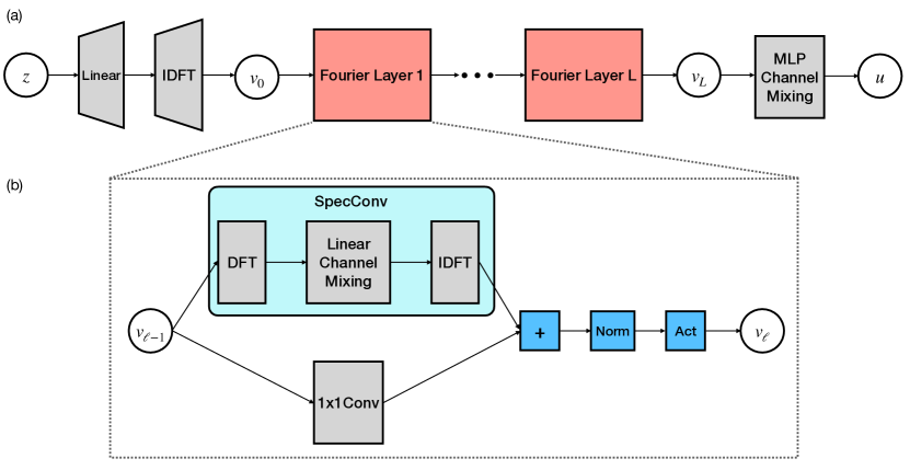
Figure 3: (a) Network architecture of the decoder $D_{\gamma}$. Starting from $z\in\mathbbm{R}^{d_{z}}$ in a low-dimensional latent space, we first apply a complex linear layer followed by an IDFT to lift it to $v_{0}\in\mathbbm{R}^{d_{u}}$ in a high-dimensional state space. We then apply $L$ Fourier layers iteratively to get $v_{L}\in\mathbbm{R}^{n_{L}\times d_{u}}$ where $n_{L}$ is the channel dimension. We project it back to the state space by applying a two-layer fully-connected NN to mix the channels and output $u\in\mathbbm{R}^{d_{u}}$. (b) Fourier layer: The design was first proposed in [56], and we describe it here for the sake of completeness. The upper half represents a spectral convolutional layer, where we transform the input $v_{\ell-1}\in\mathbbm{R}^{n_{\ell-1}\times d_{u}}$ into the frequency space with DFT, mix the channels with a complex linear map, and transform back with IDFT. The lower half is a one-by-one convolutional layer, which is a generalization of residual connection. The outputs from both layers are summed up and passed through a normalization and an activation layer to produce the output $v_{\ell}\in\mathbbm{R}^{n_{\ell}\times d_{u}}$.

4.2 Algorithmic Design for Computational Efficiency

If the time-window length $T$ is large, we follow [20] and use truncated backpropagation to auto-differentiate the map $\theta\mapsto\mathcal{L}_{{\footnotesize\text{EnKF}}}(\theta)$: we divide the sequence into multiple short subsequences and backpropagate within each subsequence. The idea stems from Truncated Backpropagation Through Time (TBPTT) for RNNs [93, 82] and the recursive maximum likelihood method for hidden Markov models [53]. By doing so, multiple gradient ascent steps can be performed for each single filtering pass, and thus the data can be utilized more efficiently. Moreover, gradient explosion/vanishing [3] are less likely to happen. We refer to [20] for more details. We choose this variant of ROAD-EnKF in our experiments.

In this work we are mostly interested in the case where $d_{u}$ and $d_{y}$ are large, and $d_{z}$ is small. Moreover, the ensemble size $N$ that we consider is moderate, i.e., $d_{u}\geq d_{y}>N>d_{z}$. Therefore, we do not pursue the covariance localization approach as in [20] (see also [43, 38]), which is most effective when $N<d_{z}$. Instead, we notice that the computational bottlenecks of the analysis step in the EnKF Algorithm 3.1 are the $O(d_{y}^{3})$ operations of computing the Kalman gain (5) as well as updating the data log-likelihood (7), where we need to compute the matrix inverse and log-determinant of a $d_{y}\times d_{y}$ matrix $(\widehat{C}_{yy,t}+R_{t})$. If $d_{y}>N$, the number of operations can be improved to $O(N^{3})$ as follows. Let $Y_{t}\in\mathbbm{R}^{d_{y}\times N}$ be the matrix representation of the centered ensemble after applying the observation function, i.e., its $n$-th column is $Y_{t}^{n}:=\frac{1}{\sqrt{N-1}}\big{(}\mathcal{H}_{\gamma,t}(\widehat{z}_{t}^{n})-\frac{1}{N}\sum_{m=1}^{N}\mathcal{H}_{\gamma,t}(\widehat{z}_{t}^{m})\big{)}$ (we drop the parameter $\gamma$ for convenience). This leads to $\widehat{C}_{yy,t}=Y_{t}Y_{t}^{\top}$. By the matrix inversion lemma [94],

$$(\widehat{C}_{yy,t}+R_{t})^{-1}=R_{t}^{-1}-R_{t}^{-1}Y_{t}(I+Y_{t}^{\top}R_{t}^{-1}Y_{t})^{-1}Y_{t}^{\top}R_{t}^{-1},$$ (4.3)

$${\text{logdet}}(\widehat{C}_{yy,t}+R_{t})={\text{logdet}}(I+Y_{t}^{\top}R_{t}^{-1}Y_{t})+{\text{logdet}}(R_{t}),$$ (4.4)

where $I+Y_{t}^{\top}R_{t}^{-1}Y_{t}\in\mathbbm{R}^{N\times N}$. The computational cost can be further reduced if the quantities $R_{t}^{-1}$ and ${\text{logdet}}(R_{t})$ can be pre-computed, for instance when $R_{t}=rI$ for some scalar $r\in\mathbbm{R}$.

Moreover, in practice, to update the ensemble in 6 of Algorithm 3.1, instead of inverting $I+Y_{t}^{\top}R_{t}^{-1}Y_{t}$ directly in 4.3 followed by a matrix multiplication, we find it more numerically stable to first solve the following linear system:

$$(I+Y_{t}^{\top}R_{t}^{-1}Y_{t})u_{t}^{n}=Y_{t}^{\top}R_{t}^{-1}\big{(}y_{t}+\gamma_{t}^{n}-\mathcal{H}_{\gamma,t}(\widehat{z}_{t}^{n})\big{)}$$ (4.5)

for $u_{t}^{n}\in\mathbbm{R}^{N}$, and then perform the analysis step (6 of Algorithm 3.1) by

$$\begin{split}z_{t}^{n}&=\widehat{z}_{t}^{n}+\widehat{C}_{zy,t}(\widehat{C}_{yy,t}+R_{t})^{-1}\big{(}y_{t}+\gamma_{t}^{n}-\mathcal{H}_{\gamma,t}(\widehat{z}_{t}^{n})\big{)}\\ &=\widehat{z}_{t}^{n}+\widehat{C}_{zy,t}\big{(}R_{t}^{-1}-R_{t}^{-1}Y_{t}(I+Y_{t}^{\top}R_{t}^{-1}Y_{t})^{-1}Y_{t}^{\top}R_{t}^{-1}\big{)}\big{(}y_{t}+\gamma_{t}^{n}-\mathcal{H}_{\gamma,t}(\widehat{z}_{t}^{n})\big{)}\\ &=\widehat{z}_{t}^{n}+\widehat{C}_{zy,t}R_{t}^{-1}\big{(}y_{t}+\gamma_{t}^{n}-\mathcal{H}_{\gamma,t}(\widehat{z}_{t}^{n})-Y_{t}u_{t}^{n}\big{)}.\end{split}$$ (4.6)

Similar ideas and computational cost analysis can be found in [85]. For the benchmark experiments in Section 5, we modify the AD-EnKF algorithm as presented in [20] to incorporate the above ideas.

4.3 Latent Space Regularization

Since the estimation of $u$ is given by $D_{\gamma}(z),$ where both $D_{\gamma}(\cdot)$ and $z$ need to be identified from data, we overcome potential identifiability issues by regularizing $z$ in the latent space. To further motivate the need for latent space regularization, consider the following example: if the pair $(z,D_{\gamma}(\cdot))$ provides a good estimation of $u_{t}$, then so does $(cz,\frac{1}{c}D_{\gamma}(\cdot))$ for any constant $c\neq 0$. Therefore, the norm of $z$ can be arbitrarily large, and thus we regularize $z$’s in the latent space so that their norms do not explode.

We perform regularization by extending the observation model 2.11 to impose additional constraints on the latent state variable $z_{t}$’s. The idea stems from regularization in ensemble Kalman methods for inverse problems [15, 37]. We first extend 2.11 to the equations:

$$\left\{\begin{array}[]{@{}r @{}l @{}l }y_{t}&\,=\mathcal{H}_{\gamma,t}(z_{t})+\eta_{t},&\eta_{t}\sim\mathcal{N}(0,R_{t}),\\ 0&\,=z_{t}+\epsilon_{t},&\epsilon_{t}\sim\mathcal{N}(0,\sigma^{2}I_{d_{z}}),\end{array}\right.$$ (4.7)

where $\sigma$ is a parameter to be chosen that incorporates the prior information that each coordinate of $z_{t}$ is an independent centered Gaussian random variable with standard deviation $\sigma$. Define

$$y_{t}^{\text{aug}}=\begin{bmatrix}y_{t}\\ 0\end{bmatrix},\quad\quad\mathcal{H}_{\gamma,t}^{\text{aug}}(z_{t})=\begin{bmatrix}\mathcal{H}_{\gamma,t}(z_{t})\\ z_{t}\end{bmatrix},\quad\quad\eta_{t}^{\text{aug}}\sim\mathcal{N}(0,R_{t}^{\text{aug}}),\quad\quad R_{t}^{\text{aug}}=\begin{bmatrix}R_{t}&0\\ 0&\sigma^{2}I_{d_{z}}\end{bmatrix}.$$ (4.8)

We then write 4.7 into an augmented observation model

$$y_{t}^{\text{aug}}=\mathcal{H}_{\gamma,t}^{\text{aug}}(z_{t})+\eta_{t}^{\text{aug}},\quad\quad\eta_{t}^{\text{aug}}\sim\mathcal{N}(0,R_{t}^{\text{aug}}).$$ (4.9)

To perform latent space regularization in ROAD-EnKF, during the training stage we run EnKF (Line 6 of Algorithm 3.2) with augmented data $y_{1:T}^{\text{aug}}$ and SSM with the augmented observation model, i.e., (2.10)-(4.9)-(2.12). During test stage, we run EnKF (Line 11 of Algorithm 3.2) with the original data and SSM, i.e., (2.10)-(2.11)-(2.12).

5 Numerical Experiments

In this section, we compare our ROAD-EnKF method to the SINDy autoencoder [16], which we abbreviate as SINDy-AE. It learns an encoder-decoder pair that maps between observation space ($y_{t}$’s) and latent space ($z_{t}$’s), and simultaneously performs a sparse dictionary learning in the latent space to discover the latent dynamics. Similar to SINDy-AE, our ROAD-EnKF method jointly discovers a latent space and the dynamics therein that is a low-dimensional representation of the data. However, our method differs from SINDy-AE in four main aspects: (1) No time-derivative data for $y_{1:T}$ are required; (2) No encoder is required; (3) State reconstruction and forecast can be performed even when the data $y_{1:T}$ are noisy and partial observation of $u_{1:T}$, while SINDy-AE is targeted at noiseless and fully observed data that are dense in time; (4) Stochastic representation of latent dynamics model can be learned, and uncertainty quantification can be performed in state reconstruction and forecast tasks through the use of particles, while SINDy-AE only provides a point estimate in both tasks.

We also compare our ROAD-EnKF method to AD-EnKF [20]. Although AD-EnKF enjoys some of the benefits of ROAD-EnKF, including the capability to learn from noisy, partially observed data and perform uncertainty quantification, it directly learns the dynamics model in high-dimensional state space (i.e., on $u_{t}$’s instead of $z_{t}$’s), which leads to higher model complexity, as well as additional computational and memory costs when performing the EnKF step. Moreover, AD-EnKF does not take advantage of the possible low-dimensional representation of the state. We compare in Table 5.1 below the capabilities of the three algorithms under different scenarios.

	Learn from noisy and partially observed data	Uncertainty quantification	No need of time-derivative data	Low-dimensional state representation
SINDy-AE[16]	✗	✗	✗	✓
AD-EnKF[20]	✓	✓	✓	✗
ROAD-EnKF (this paper)	✓	✓	✓	✓

Table 5.1: Comparison of SINDy-AE, AD-EnKF, and ROAD-EnKF under different scenarios.

Other alternative methods include EnKF-embedded EM algorithms (e.g. [9]) and autodifferentiable PF algorithms (e.g., [65]). Since [20] already establishes AD-EnKF’s superiority to those approaches, we do not include them in these experiments, and we refer to [20] for more details.

The training procedure is the following: We first specify a forecast lead time $T_{f}$. We then generate training data $y_{0:T}^{\mathcal{I}_{\footnotesize\text{train}}}$ and test data with extended time range $(u_{0:T+T_{f}}^{\mathcal{I}_{\footnotesize\text{test}},\ast},y_{0:T}^{\mathcal{I}_{\footnotesize\text{test}}})$ with $N_{\footnotesize\text{train}}:=|\mathcal{I}_{\footnotesize\text{train}}|$ and $N_{\footnotesize\text{test}}:=|\mathcal{I}_{\footnotesize\text{test}}|$. The data are either generated from a reduced-order SSM 2.6-2.9 with explicit knowledge of true parameter $\theta$ (Subsection 5.1), or from an SSM 2.1-2.3 with no explicit knowledge of the exact reduced-order structure (Subsections 5.2 and 5.3). The data $y_{0:T}^{\mathcal{I}_{\footnotesize\text{train}}}$ and $y_{0:T}^{\mathcal{I}_{\footnotesize\text{test}}}$ are then passed into ROAD-EnKF (Algorithm 3.2), and we evaluate the following:

Reconstruction-RMSE (RMSE-r):

Measures the state reconstruction error of the algorithm. We take the particle mean of $u_{0:T}^{\mathcal{I}_{\footnotesize\text{test}},1:N}$ as a point estimate of the true states $u_{0:T}^{\mathcal{I}_{\footnotesize\text{test}},\ast}$, and evaluate the RMSE:

$$\text{RMSE-r}=\sqrt{\frac{1}{d_{u}N_{\footnotesize\text{test}}(T-T_{b})}\sum_{t=T_{b}}^{T}\sum_{i\in\mathcal{I}_{\footnotesize\text{test}}}\Big{|}\overline{u}_{t}^{i}-u_{t}^{i,\ast}\Big{|}^{2}}\,,\quad\quad\text{where }\,\overline{u}_{t}^{i}=\frac{1}{N}\sum_{n=1}^{N}u_{t}^{i,n}.$$ (5.1)

Here $T_{b}$ is a number of burn-in steps to remove transient errors in the reconstruction that stem from the choice of initialization. For simplicity, we set $T_{b}=\lfloor T/5\rfloor$ as in [20].

Forecast-RMSE (RMSE-f):

Measures the $t$-step state forecast error of the algorithm, for lead time $t\in\{1,\ldots,T_{f}\}$. We take the particle mean of $u_{T+t}^{\mathcal{I}_{\footnotesize\text{test}},1:N}$ as a point estimate of the true future states $u_{T+t}^{\mathcal{I}_{\footnotesize\text{test}},\ast}$:

$$\text{RMSE-f}(t)=\sqrt{\frac{1}{d_{u}N_{\footnotesize\text{test}}}\sum_{i\in\mathcal{I}_{\footnotesize\text{test}}}\Big{|}\overline{u}_{T+t}^{i}-u_{T+t}^{i,\ast}\Big{|}^{2}}\,,\quad\quad\text{where }\,\overline{u}_{T+t}^{i}=\frac{1}{N}\sum_{n=1}^{N}u_{T+t}^{i,n}\,.$$ (5.2)

Test Log-Likelihood:

Measures the averaged log-likelihood of the learned reduced-order SSM over test observation data $y_{0:T}^{\mathcal{I}_{\footnotesize\text{test}}}$, which is $\mathcal{L}_{{\footnotesize\text{EnKF}}}(\theta^{k})$ defined in 11 of Algorithm 3.2.

For AD-EnKF, the above metrics can be similarly computed, following [20]. For SINDy-AE, as uncertainty quantification is not performed, we use its decoder output as the point estimate of the state in both reconstruction and forecast. Moreover, log-likelihood computation is not available for SINDy-AE.

5.1 Embedding of Chaotic Dynamics (Lorenz 63)

In this subsection, we reconstruct and forecast a state defined by embedding a Lorenz 63 (L63) model in a high-dimensional state space. A similar experiment was used in [16] to motivate the SINDy-AE algorithm, and hence this example provides a good point of comparison. The data are generated using the L63 system as the true latent state dynamics model:

$$\frac{\text{d}z}{\text{d}s}=g(z),\quad\quad\begin{cases}g^{(1)}(z)=10(z^{(2)}-z^{(1)}),\\ g^{(2)}(z)=z^{(1)}(28-z^{(3)})-z^{(2)},\\ g^{(3)}(z)=z^{(1)}z^{(2)}-\frac{8}{3}z^{(3)},\end{cases}\quad\quad G:z(s)\mapsto z(s+\Delta_{s}),$$ (5.3)

where $z^{(i)}$ and $g^{(i)}$ denote the $i$-th coordinate of $z$ and component of $g$, and $\Delta_{s}$ is the time between observations. We further assume there is no noise in the true latent state dynamics model, i.e., $S=0$. To construct the true reduced-order SSM, we define $D\in\mathbbm{R}^{d_{u}\times 6}$ such that its $i$-th column $D^{i}\in\mathbbm{R}^{d_{u}}$ is given by the discretized $i$-th Legendre polynomial over $d_{u}$ grid points. The true states $u_{t}\in\mathbbm{R}^{d_{u}}$ are defined by

$$u_{t}:=D\begin{bmatrix}z_{t}^{(1)}/40&z_{t}^{(2)}/40&z_{t}^{(3)}/40&(z_{t}^{(1)}/40)^{3}&(z_{t}^{(2)}/40)^{3}&(z_{t}^{(3)}/40)^{3}&\end{bmatrix}^{\top}.$$ (5.4)

We consider two cases of the observation model (2.8): (1) full observation, where all coordinates of $u_{t}$ are observed, i.e., $H_{t}=I_{d_{u}}$ and $d_{y}=d_{u}$; (2) partial observation, where for each $t$, only a fixed portion $c<1$ of all coordinates of $u_{t}$ are observed, and the coordinate indices are chosen randomly without replacement. In this case, $H_{t}\in\mathbbm{R}^{d_{y}\times d_{u}}$ is a submatrix of $I_{d_{u}}$ and varies across time, and $d_{y}=cd_{u}$. This partial observation set-up has been studied in the literature (e.g., [9, 7]) for data assimilation problems. For both cases, we assume $R_{t}=0.01I_{d_{y}}$ and $z_{0}\sim\mathcal{N}(0,4I_{d_{z}})$.

We consider full observation with $d_{u}=d_{y}=128$ and partial observation with $d_{u}=128$, $d_{y}=64$ (i.e., $c=1/2$). We generate $N_{\footnotesize\text{train}}=1024$ training data and $N_{\footnotesize\text{test}}=20$ test data with the true reduced-order SSM defined by (5.3) and (5.4). We set the number of observations $T=250$ with time between observations $\Delta_{s}=0.1$. We set the forecast lead time $T_{f}=10$. The latent flow map $G$ is integrated using the Runge–Kutta–Fehlberg method. The surrogate latent dynamics map $g_{\alpha}$ is parameterized as a two-layer fully connected NN, and is integrated using a fourth-order Runge-Kutta method with step size $\Delta_{s}^{\text{int}}=0.05$. The error covariance matrix $S_{\beta}$ in the latent dynamics is parametrized using a diagonal matrix with positive diagonal elements $\beta\in\mathbbm{R}^{d_{z}}$. The decoder $D_{\gamma}$ is parameterized as a Fourier Neural Decoder (FND) discussed in Subsection 4.1. Details of the network hyperparameters for this and subsequent examples are summarized in Table 5.2, obtained through cross-validation experiments on the training dataset. The latent space dimension for both SINDy-AE and ROAD-EnKF is set to $d_{z}=3$. The ensemble size for both AD-EnKF and ROAD-EnKF is set to $N=100$.

		L63	Burgers	KS
FND	$L$	4	2	4
	$h$	6	40	40
	$(n_{0},\dots,n_{L})$	(1, 20, 20, 20, 20)	(1, 20, 20)	(1, 20, 20, 20, 20)
	Norm	LayerNorm
	Activation	ReLU
Latent space reg.	$\sigma$	2	4	4
Optimization	Optimizer	Adam
	Learning rate ($\eta$)	1e-3
	Batch size ($B$)	16	4	4
	TBPTT length	10

Table 5.2: Choices of hyperparameters for ROAD-EnKF on different numerical examples.

In Table 5.3 we list the performance metrics of each method with full and partial observation. The state reconstruction and forecast performance on a single instance of test data are plotted in Figure 4 and 5 for the full observation case, and in Figure 6 for the partial observation case. For the full observation case, we compare ROAD-EnKF with AD-EnKF and SINDy-AE, adopting for the latter the implementation in [16]. Since SINDy-AE requires time-derivative data as input, we use a finite difference approximation computed from data $y_{1:T}$. We also include the results for SINDy-AE where the exact time-derivative data are used. We find that ROAD-EnKF is able to reconstruct and forecast the states consistently with the lowest RMSE, and the performance is not affected by whether the state is fully or partially observed. AD-EnKF is able to reconstruct and forecast the state with a higher RMSE than that of ROAD-EnKF, and the performance deteriorates in the partially observed setting. SINDy-AE with finite difference approximation of derivative data also achieves higher reconstruction RMSE than that of ROAD-EnKF, and does not give accurate state forecasts. This is likely due to the fact that data are sparse in time (i.e., $\Delta_{s}$ is large) which leads to a larger error when approximating the true time-derivative, and hence it is more difficult to extract meaningful dynamics from the data. Even when the true time-derivative data are used (which is not available unless we have explicit knowledge of the true reduced-order SSM), SINDy-AE has a higher reconstruction RMSE compared to ROAD-EnKF, and its forecast performance is still worse than the other two methods. Moreover, it cannot handle partial observation.

In terms of computational cost, ROAD-EnKF is more efficient than AD-EnKF since the surrogate dynamics are cheaper to simulate and the EnKF algorithm is more efficient to perform in both training and testing. However, ROAD-EnKF takes more time than SINDy-AE, since the latter does not rely on a filtering algorithm, but rather an encoder, to reconstruct the states and perform learning.

	SINDy-AE (full)	SINDy-AE (w/ derivative, full)	AD-EnKF (full)	ROAD-EnKF (full)	AD-EnKF (partial)	ROAD-EnKF (partial)
RMSE-r	0.0142	0.0148	0.0168	0.0078	0.0368	0.0079
RMSE-f(1)	0.1310	0.0191	0.0156	0.0069	0.0315	0.0069
RMSE-f(5)	1.6580	0.0333	0.0335	0.0141	0.0729	0.0125
Log-likelihood	$-$		$2.25\times 10^{4}$	$2.58\times 10^{4}$	$1.28\times 10^{4}$	$1.40\times 10^{4}$
Training time (per epoch)	5.15s		9.74s	6.15s	8.86s	5.62s
Test time	2.35s		4.57s	2.95s	4.52s	2.73s

Table 5.3: Performance metrics for different algorithms at convergence. (Embedded L63 example, Subsection 5.1.)

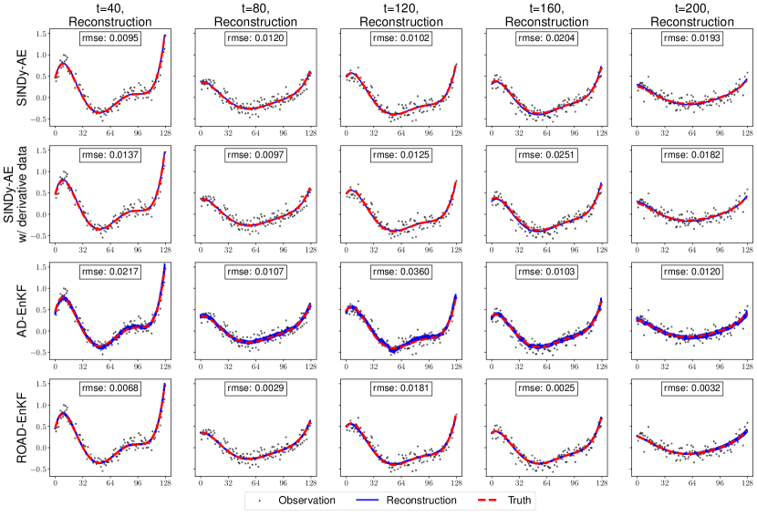
Figure 4: State reconstruction performance with full observation ($d_{u}=d_{y}=128$) on the embedded L63 example in Subsection 5.1. For each method (row), the reconstructed states $u_{t}$ (blue) for a single test sequence are plotted for $t=40,80,120,160,200$ (column). The true values of the 128-dimensional states are plotted in red dashed lines, along with the noisy observations in black dots. Both AD-EnKF and ROAD-EnKF perform probabilistic state reconstructions through particles (all plotted in blue), while SINDy-AE only provides point estimates. The reconstruction RMSE’s are computed for each plot. For SINDy-AE, even with derivative data (not required for AD-EnKF and ROAD-EnKF), the reconstruction performance is similar to that of AD-EnKF, while being worse than that of ROAD-EnKF.

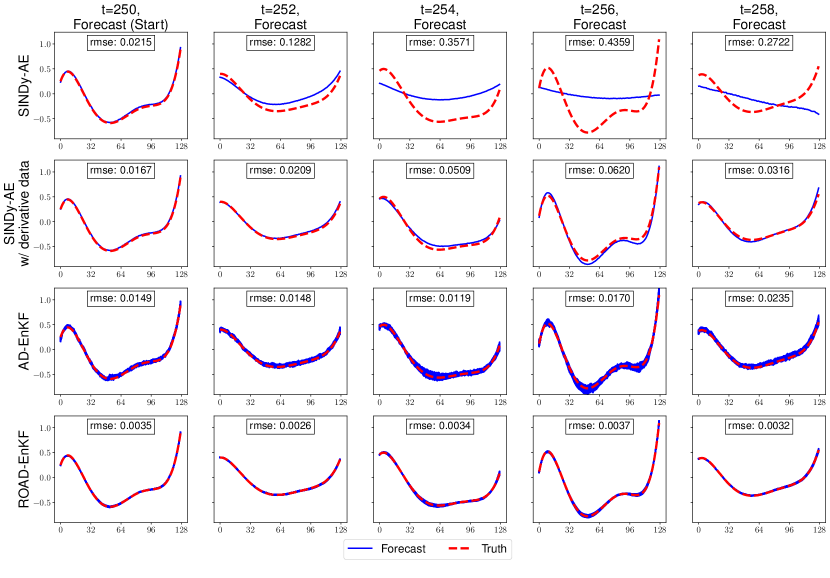
Figure 5: Forecast performance with full observation ($d_{u}=d_{y}=128$) on the embedded L63 example in Subsection 5.1. For each method (row), the forecasted states $u_{t}$ (blue) for a single test sequence are plotted for $t=250$ (start of forecast), $252,254,256,258$ (column). The true values of the $d_{u}=128$ dimensional states are plotted in red dashed lines. Both AD-EnKF and ROAD-EnKF perform probabilistic forecast through particles (all plotted in blue), while SINDy-AE only provides point estimates. The forecast RMSE’s are computed for each plot. For SINDy-AE, even with derivative data (not required for AD-EnKF and ROAD-EnKF), the forecast performance is similar to that of AD-EnKF, while being worse than that of ROAD-EnKF.

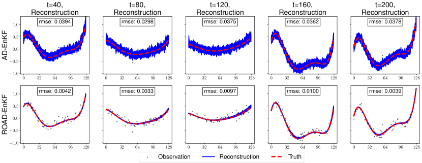
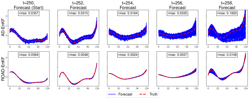
Figure 6: State reconstruction (upper half) and forecast (lower half) performance with partial observation ($d_{u}=128$, $d_{y}=64$) on the embedded L63 example in Subsection 5.1. For each method, the reconstructed states $u_{t}$ (blue) for a single test sequence are plotted for $t=40,80,120,160,200$ (column), and the forecasted states $u_{t}$ (blue) for a single test sequence are plotted for $t=250$ (start of forecast), $252,254,256,258$ (column). The true values of the 128-dimensional states are plotted in red dashed lines, along with the noisy observations in black dots. SINDy-AE is inapplicable here because it cannot handle partial observations, while both AD-EnKF and ROAD-EnKF perform probabilistic state reconstructions and forecast through particles (all plotted in blue). The reconstruction/forecast RMSEs are computed for each plot.

5.2 Burgers Equation

In this subsection and the following one, we learn high-dimensional SSMs without explicit reference to a true model for low-dimensional latent dynamics. We first consider the 1-dimensional Burgers equation for $u(x,s)$, where $u$ is a function of the spatial variable $x\in[0,\mathsf{L}]$ and continuous-time variable $s>0$:

$$\begin{split}&\frac{\partial u}{\partial s}=-u\frac{\partial u}{\partial x}+\nu\frac{\partial^{2}u}{\partial x^{2}},\\ &u(0,s)=u(\mathsf{L},s)=0,\\ &u(x,0)=u_{0}(x).\end{split}$$ (5.5)

Here $\nu$ is the viscosity parameter, and we set $\nu=1/150$, $\mathsf{L}=2$. Burgers equation [11] has various applications in fluid dynamics, including modeling of viscous flows. We are interested in reconstructing solution states, as well as in the challenging problem of forecasting shocks that emerge outside the time range covered by the training data. Equation 5.5 is discretized on $[0,\mathsf{L}]$ with equally-spaced grid points $0=x_{1}<x_{2}<\cdots<x_{M}=\mathsf{L}$, using a second-order finite difference method. Setting $\Delta x:=x_{i}-x_{i-1}=\frac{\mathsf{L}}{M-1}$, we obtain the following ODE system:

$$\begin{split}&\frac{\text{d}u^{(i)}}{\text{d}s}=-\frac{\big{(}u^{(i+1)}\big{)}^{2}-\big{(}u^{(i-1)}\big{)}^{2}}{4\Delta x}+\nu\frac{u^{(i+1)}-2u^{(i)}+u^{(i-1)}}{\Delta x^{2}},\quad\quad i=2,\dots,M-1,\\ &u^{(1)}(s)=u^{(M)}(s)=0,\\ &u^{(i)}(0)=u_{0}(i\Delta x).\end{split}$$ (5.6)

Here $u^{(i)}(s)$ is an approximation of $u(i\Delta x,s)$, the value of $u$ at the $i$-th spatial node at time $s$. Equation 5.6 defines a flow map $F:u(s)\mapsto u(s+\Delta_{s})$ for state variable $u$ with $d_{u}=M$, which we refer to as the true state dynamics model. We assume there is no noise in the dynamics, i.e., $Q=0$.

Similar to Subsection 5.1, we consider two cases: full observation with $d_{u}=d_{y}=256$ and partial observation with $d_{u}=256$, $d_{y}=128$ (i.e., $c=1/2$). The initial conditions $u_{0}$ are generated in the following way:

$$u_{0}^{(i)}=U\sin\frac{2\pi i\Delta x}{\mathsf{L}},\quad\quad U\sim\text{Uniform}(0.5,1.5).$$ (5.7)

We generate $N_{\footnotesize\text{train}}=1024$ training data and $N_{\footnotesize\text{test}}=20$ test data with the true state dynamics model defined through equation 5.6 and 5.7 with $R_{t}=0.01I_{d_{y}}$. We set the number of observations $T=300$ with time between observations $\Delta_{s}=0.001$. We set the forecast lead time $T_{f}=300$. The flow map $F$ is integrated using the fourth-order Runge–Kutta method with a fine step size $\Delta_{s}/20$. The surrogate latent dynamics map $g_{\alpha}$ is parameterized as a two-layer fully connected NN, and is integrated using a fourth-order Runge-Kutta method with step size $\Delta_{s}^{\text{int}}=0.001$. The error covariance matrix $S_{\beta}$ in the latent dynamics is parametrized using a diagonal matrix with positive diagonal elements $\beta\in\mathbbm{R}^{d_{z}}$. The decoder $D_{\gamma}$ is parameterized as an FND, discussed in Subsection 4.1. Details of the network hyperparameters are listed in Table 5.2. The latent space dimension for ROAD-EnKF is set to $d_{z}=40$. The ensemble size for both AD-EnKF and ROAD-EnKF is set to $N=100$. In this example and the following one, we set $z_{0}\sim\mathcal{N}(0,\sigma^{2}\mathcal{I}_{d_{z}})$ with the same $\sigma$ defined in Subsection 4.3.

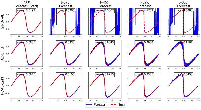
Figure 11: State reconstruction (upper half) and forecast (lower half) performance with full observation ($d_{u}=d_{y}=256$) on the Burgers example in Subsection 5.2. For each method, the reconstructed states $u_{t}$ (blue) for a single test sequence are plotted for $t=50,100,150,200,250$ (column), and the forecasted states (blue) for a single test sequence are plotted for $t=300$ (start of forecast), $375,450,525,600$ (column). The true values of the 256-dimensional states are plotted in red dashed lines, along with the noisy observations in black dots. Both AD-EnKF and ROAD-EnKF perform probabilistic state reconstructions and forecast through particles (all plotted in blue), while SINDy-AE only provides point estimates. The reconstruction/forecast RMSEs are computed for each plot.

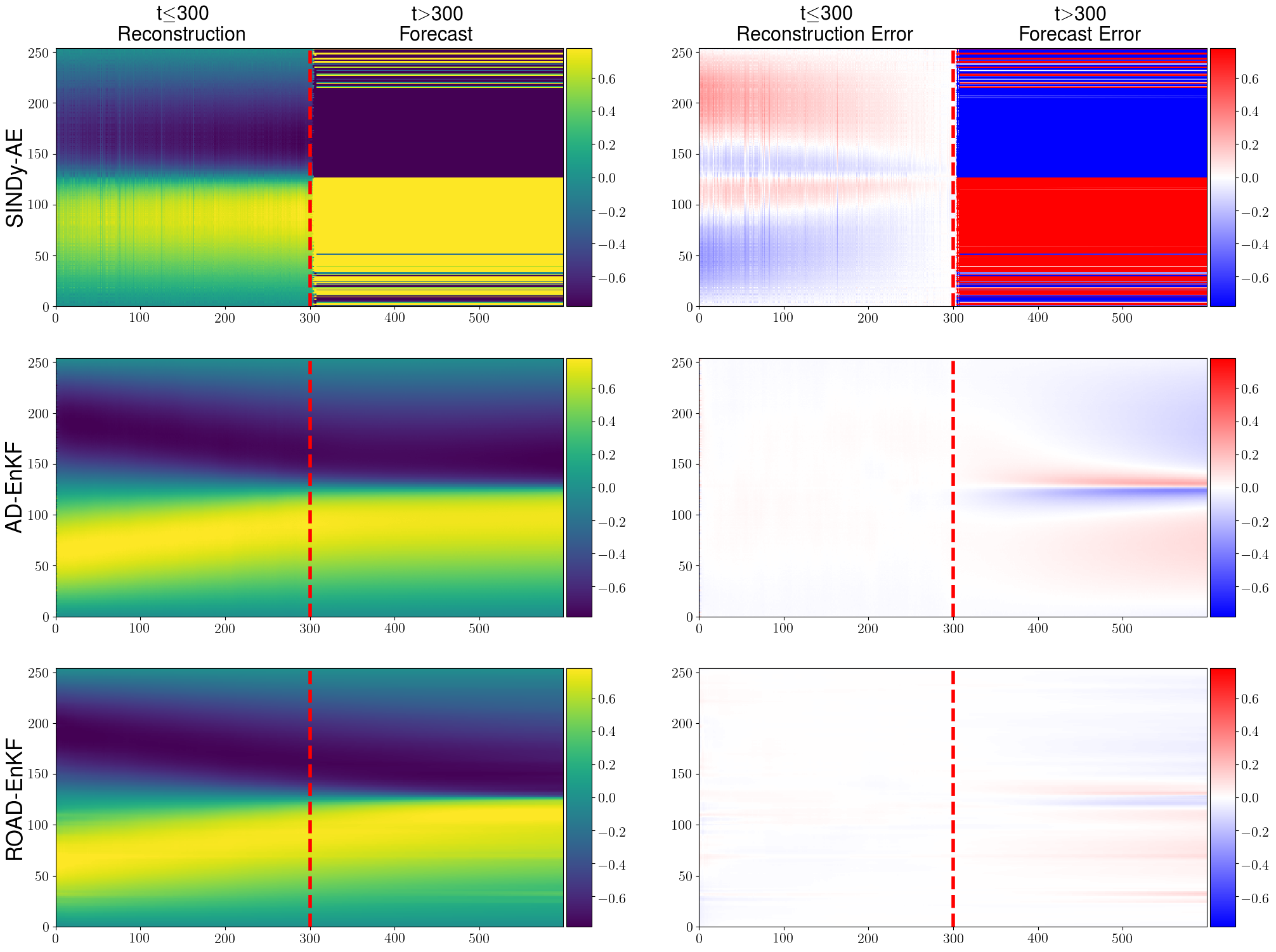
(b) Reconstruction and forecast.

Figure 12: Contour plot of state reconstruction and forecast output with full observation ($d_{u}=d_{y}=256$) on the Burgers example in Subsection 5.2, as well as the ground truth (top). For each method (row), the reconstructed and forecasted states (left column) for a single test sequence are plotted, for each state dimension (y-axis) and time (x-axis). The error compared to the ground truth are plotted in the right column. For both AD-EnKF and ROAD-EnKF we use particle means as point estimates.

In Table 5.4, we list the performance metrics of each method with full and partial observation. The state reconstruction and forecast performance on a single instance of test data are plotted in Figures 7 (snapshots) and 8 (contour plot) for the partial observation case. Corresponding plots with full observation are shown in Figures 11 and 12 in the appendix. We find that ROAD-EnKF is able to reconstruct and forecast the states with the lowest RMSE, in both full and partial observation scenarios. More importantly, the emergence of shocks is accurately forecasted even though this phenomenon is not included in the time range covered by the training data. AD-EnKF achieves a higher RMSE than ROAD-EnKF for both state reconstruction and forecast tasks. AD-EnKF forecasts the emergence of shocks with lower accuracy than ROAD-EnKF, which indicates that AD-EnKF fails to fully learn the state dynamics. SINDy-AE with finite difference approximation of derivative data has the highest reconstruction RMSE among the three methods, and is not able to produce meaningful long-time state forecasts. This is remarkable, given that in this example the data are relatively dense ($\Delta_{s}$ is small) which facilitates, in principle, the approximation of time derivatives. In terms of computational cost, ROAD-EnKF is more efficient than AD-EnKF during both training and testing, but takes more time than SINDy-AE for the same reason as in Subsection 5.1.

In Table 5.5, we list the performance metrics of ROAD-EnKF with full observation and different choices of latent space dimension $d_{z}$ ranging from 1 to 240. The results for partial observation show a similar trend and are not shown. We find that, as $d_{z}$ increases, the state reconstruction performance stabilizes when $d_{z}\geq 4$. In order to achieve better long-time state forecast performance, $d_{z}$ needs to be further increased, and the forecast performance stabilizes when $d_{z}\geq 10$. Both training and testing time slightly increase as $d_{z}$ grows, which can be explained by the following: The computational time for both training and testing can be divided into the prediction step and the analysis step. We have shown in Subsection 4.2 that the computational bottleneck of the analysis step depends on the choices of ensemble size $N$ and $d_{y}$, and is less affected by the increase of $d_{z}$. Moreover, the computational time of the prediction step depends on the complexity of the surrogate latent dynamics (two-layer NNs), which are relatively cheap to simulate for ROAD-EnKF. On the other hand, AD-EnKF enjoys similar computational complexity as ROAD-EnKF during the analysis step, but requires a more complicated surrogate model (NNs with Fourier layers) to capture the dynamics, which is more expensive to simulate. More experimental results on different parameterization methods of surrogate dynamics can be found in Table B.1 in the appendix.

	SINDy-AE (full)	AD-EnKF (full)	ROAD-EnKF (full)	AD-EnKF (partial)	ROAD-EnKF (partial)
RMSE-r	0.1433	0.0102	0.0044	0.0122	0.0081
RMSE-f(30)	4.4579	0.0212	0.0096	0.0228	0.0160
RMSE-f(150)	4.4906	0.0763	0.0514	0.0724	0.0581
Log-likelihood	$-$	$6.40\times 10^{4}$	$6.60\times 10^{4}$	$3.24\times 10^{4}$	$3.27\times 10^{4}$
Training time (per epoch)	11.78s	26.75s	12.10s	27.08s	12.20s
Test time	2.78s	11.54s	4.21s	7.76s	3.24s

Table 5.4: Performance metrics for different algorithms at convergence. (Burgers example, Subsection 5.2.)

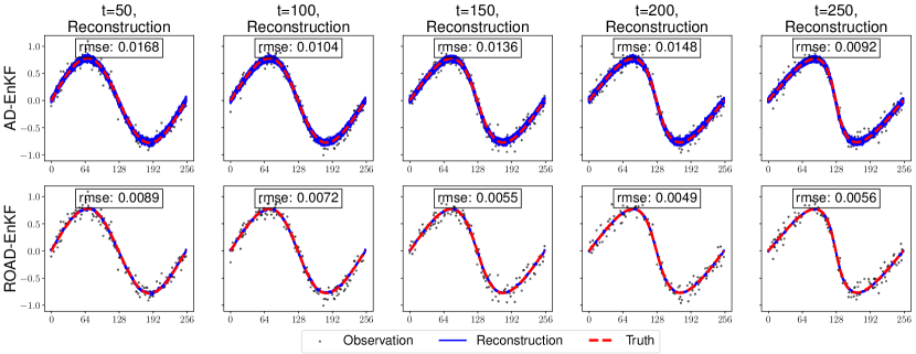
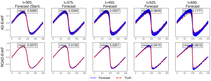
Figure 7: State reconstruction (upper half) and forecast (lower half) performance with partial observation ($d_{u}=256$, $d_{y}=128$) on the Burgers example in Subsection 5.2. For each method, the reconstructed states $u_{t}$ (blue) for a single test sequence are plotted for $t=50,100,150,200,250$ (column), and the forecasted states (blue) for a single test sequence are plotted for $t=300$ (start of forecast), $375,450,525,600$ (column). The true values of the 256-dimensional states are plotted in red dashed lines, along with the noisy observations in black dots. Both AD-EnKF and ROAD-EnKF perform probabilistic state reconstructions and forecast through particles (all plotted in blue). The reconstruction/forecast RMSEs are computed for each plot.

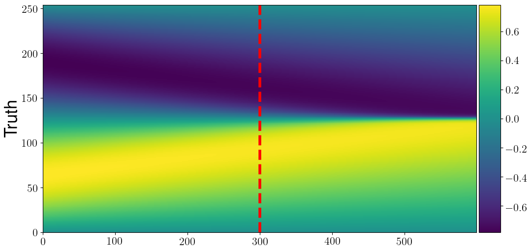
(a) Ground truth.

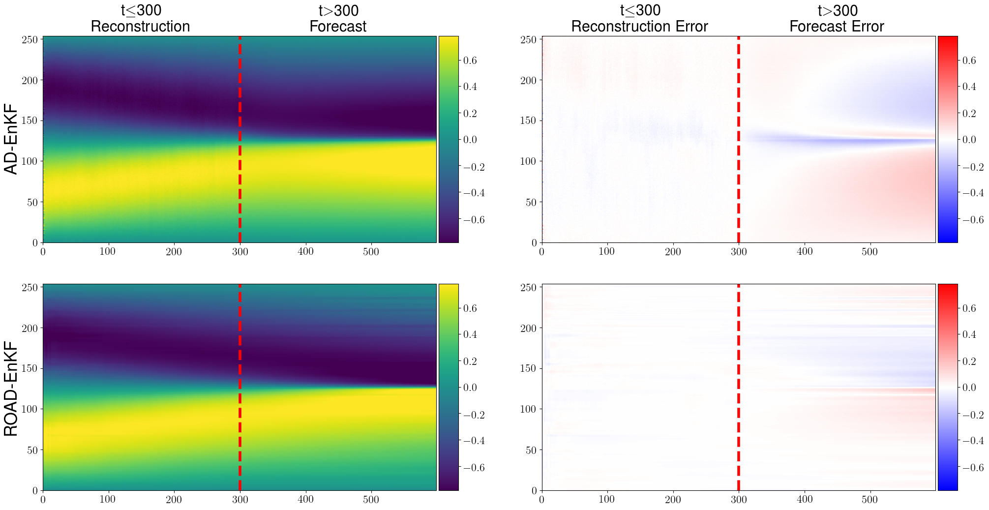
(b) Reconstruction and forecast.

Figure 8: Contour plot of state reconstruction and forecast output with partial observation ($d_{u}=256$, $d_{y}=128$) on the Burgers example in Subsection 5.2, as well as the ground truth (top). For each method (row), the reconstructed and forecasted states (left column) for a single test sequence are plotted, for each state dimension (y-axis) and time (x-axis). The error compared to the ground truth are plotted in the right column. For both AD-EnKF and ROAD-EnKF we use particle means as point estimates.

	ROAD-EnKF								AD-EnKF
	$d_{z}=1$	$d_{z}=2$	$d_{z}=4$	$d_{z}=10$	$d_{z}=20$	$d_{z}=40$	$d_{z}=120$	$d_{z}=240$
RMSE-r	0.2293	0.0316	0.0035	0.0058	0.0039	0.0044	0.0048	0.0059	0.0102
RMSE-f(30)	0.2593	0.0761	0.0165	0.0108	0.0112	0.0096	0.0100	0.0103	0.0212
RMSE-f(150)	0.2690	0.1827	0.1313	0.0501	0.0607	0.0514	0.0373	0.0382	0.0763
Log-likelihood ($\times 10^{4}$)	-14.4	6.03	6.63	6.59	6.61	6.60	6.61	6.63	6.40
Training time (per epoch)	11.70s	11.78s	11.79s	11.98s	11.98s	12.10s	12.44s	13.40s	26.75s
Test time	3.36s	3.80s	4.13s	4.14s	4.08s	4.21s	4.53s	4.90s	11.54s

Table 5.5: Performance metrics for ROAD-EnKF at convergence with full observation ($d_{u}=d_{y}=256$) and different latent space dimension $d_{z}$. (Burgers example, Subsection 5.2.)

5.3 Kuramoto-Sivashinsky Equation

In this subsection, we consider the Kuramoto-Sivashinsky (KS) equation for $u(x,s)$, where $u$ is a function of the spatial variable $x\in[0,\mathsf{L}]$ and continuous-time variable $s>0$:

$$\begin{split}&\frac{\partial u}{\partial s}=-\nu\frac{\partial^{4}u}{\partial x^{4}}-\frac{\partial^{2}u}{\partial x^{2}}-u\frac{\partial u}{\partial x},\\ &u(0,s)=u(\mathsf{L},s)=0,\\ &\frac{\partial u}{\partial x}(0,s)=\frac{\partial u}{\partial x}(\mathsf{L},s)=0,\\ &u(x,0)=u_{0}(x),\end{split}$$ (5.8)

Here $\nu$ is the viscosity parameter, and we set $\nu=0.05$, $\mathsf{L}=2$. We impose Dirichlet and Neumann boundary conditions to ensure ergodicity of the system [6]. The KS equation was originally introduced by Kuramoto and Sivashinsky to model turbulence of reaction-diffusion systems [50] and propagation of flame [77]. Equation 5.8 is discretized on $[0,\mathsf{L}]$ with equally-spaced grid points $0=x_{1}<x_{2}<\cdots<x_{M}=\mathsf{L}$, using a second-order finite difference method. Setting $\Delta x:=x_{i}-x_{i-1}=\frac{\mathsf{L}}{M-1}$, we obtain the following ODE system:

$$\begin{split}&\frac{\partial u^{(i)}}{\partial s}=-\nu\frac{u^{(i-2)}-4u^{(i-1)}+6u^{(i)}-4u^{(i+2)}+u^{(i+2)}}{\Delta x^{4}}-\frac{u^{(i+1)}-2u^{(i)}+u^{(i-1)}}{\Delta x^{2}}-\frac{\big{(}u^{(i+1)}\big{)}^{2}-\big{(}u^{(i-1)}\big{)}^{2}}{4\Delta x},\\ &\qquad\qquad\qquad\qquad\qquad\qquad\qquad\qquad\qquad\qquad\qquad\qquad\qquad\qquad\qquad\qquad\qquad\qquad i=2,\dots,d_{u}-1,\\ &u^{(1)}(s)=u^{(d_{u})}(s)=0,\\ &u^{(0)}(s)=u^{(2)}(s),u^{(d_{u}+1)}(s)=u^{(d_{u}-1)}(s),\\ &u^{(i)}(0)=u_{0}(i\Delta x).\end{split}$$ (5.9)

The discretization method follows [89]. Here $u^{(i)}(s)$ is an approximation of $u(i\Delta x,s)$, the value of $u$ at the $i$-th spatial node and time $s$. Two ghost nodes $u^{(0)}$ and $u^{(d_{u}+1)}$ are added to account for Neumann boundary conditions, and are not regarded as part of the state. Equation 5.9 defines a flow map $F:u(s)\mapsto u(s+\Delta_{s})$ for state variable $u$ with $d_{u}=M$, which we refer to as the true state dynamics model. We assume there is no noise in the dynamics, i.e., $Q=0$.

Similar to Subsection 5.1, we consider two cases: full observation with $d_{u}=d_{y}=256$ and partial observation with $d_{u}=256$, $d_{y}=128$ (i.e., $c=1/2$). The initial conditions $u_{0}$ are generated at random from the attractor of the dynamical system, by simulating a long run beforehand. We generate $N_{\footnotesize\text{train}}=512$ training data and $N_{\footnotesize\text{test}}=20$ test data with the true state dynamics model defined through 5.9 with $R_{t}=I_{d_{y}}$. We set the number of observations $T=450$ with time between observations $\Delta_{s}=0.1$. We set the forecast lead time $T_{f}=50$. The flow map $F$ is integrated using the fourth-order Runge–Kutta method with a fine step size $\Delta_{s}/10000$. The surrogate latent dynamics map $g_{\alpha}$ is parameterized as a two-layer fully connected NN, and is integrated using a fourth-order Runge-Kutta method with step size $\Delta_{s}^{\text{int}}=0.05$. The error covariance matrix $S_{\beta}$ in the latent dynamics is parametrized using a diagonal matrix with positive diagonal elements $\beta\in\mathbbm{R}^{d_{z}}$. The decoder $D_{\gamma}$ is parameterized as an FND, discussed in Subsection 4.1. Details of the network hyperparameters are listed in Table 5.2. The latent space dimension for ROAD-EnKF is set to $d_{z}=40$. The ensemble size for both AD-EnKF and ROAD-EnKF is set to $N=100$.

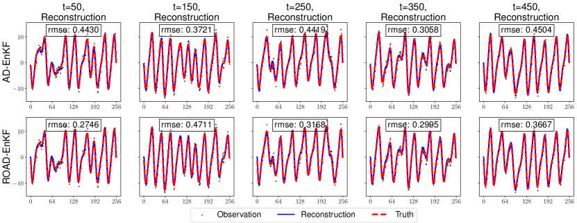
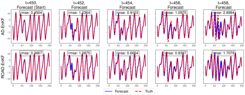
Figure 13: State reconstruction (upper half) and forecast (lower half) performance with full observation ($d_{u}=d_{y}=256$) on the KS example in Subsection 5.3. For each method, the reconstructed states $u_{t}$ (blue) are plotted for $t=50,150,250,350,450$ (column), and the forecasted states (blue) are plotted for $t=450$ (start of forecast), $452,454,456,458$ (column). The true values of the 256-dimensional states are plotted in red dashed lines, along with the noisy observations in black dots. Both AD-EnKF and ROAD-EnKF perform probabilistic state reconstructions and forecast through particles (all plotted in blue). The reconstruction/forecast RMSEs are computed for each plot.

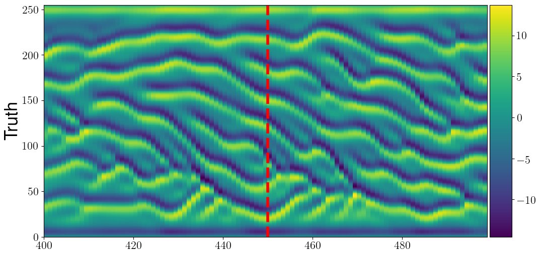
(a) Ground truth.

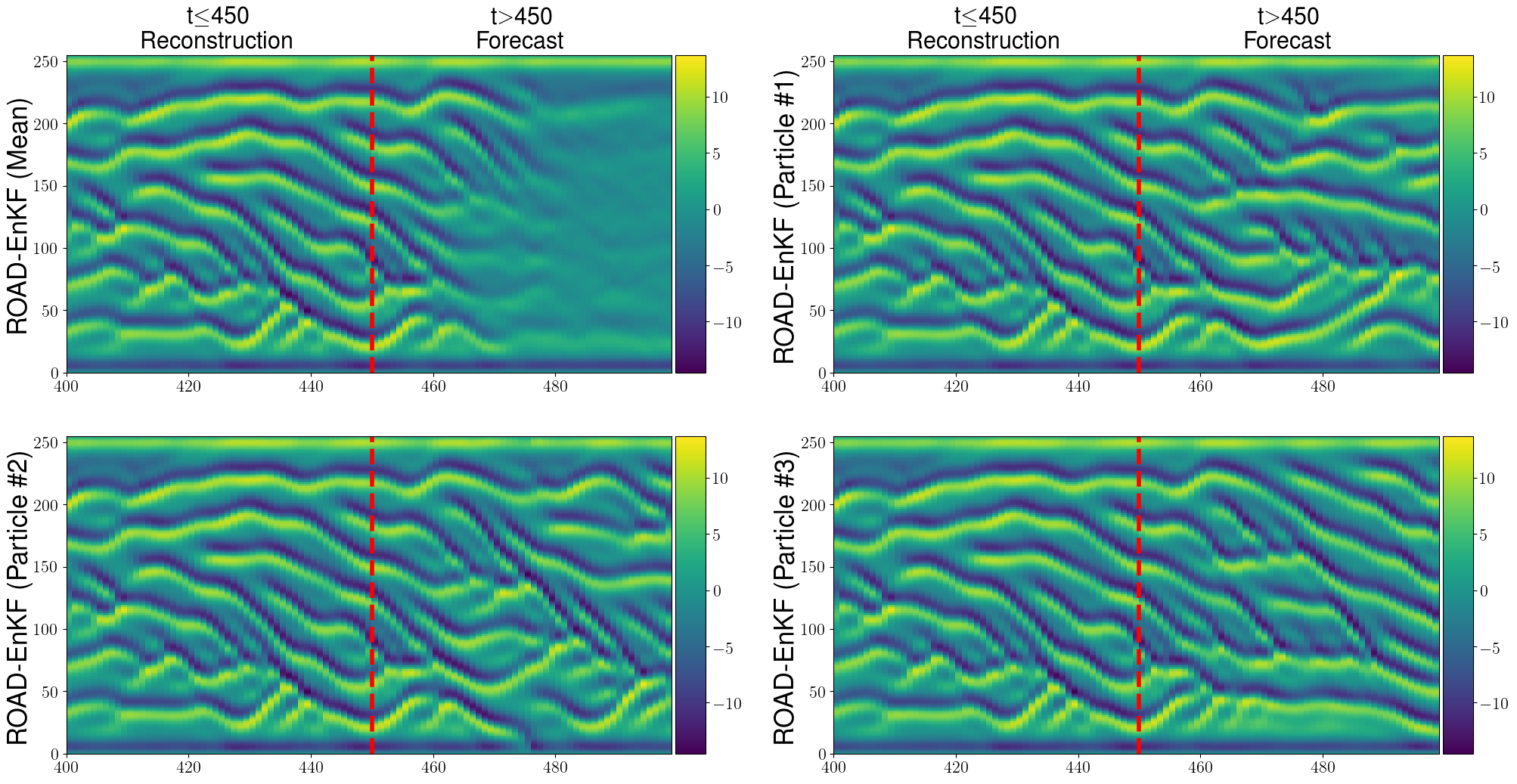
(b) Reconstruction and forecast.

Figure 14: Contour plot of state reconstruction and forecast output of ROAD-EnKF with full observation ($d_{u}=d_{y}=256$) on the KS example in Subsection 5.3, as well as the ground truth (top). The particle means of reconstructed and forecasted states are plotted, for each state dimension (y-axis) and time (x-axis). The individual reconstructed and forecasted states of three randomly chosen particles are also plotted.

In Table 5.6 we list the performance metrics of AD-EnKF and ROAD-EnKF with full and partial observation. SINDy-AE is not listed here as we find it unable to capture the dynamics for any choice of latent space dimension. The state reconstruction and forecast performance on a single instance of test data are plotted in Figure 9 (snapshots), and Figure 10 (contour plot, ROAD-EnKF) for the partial observation case. Corresponding plots with full observation are shown in Figures 13 and 14 in the appendix. We find that ROAD-EnKF is able to reconstruct the states with lower RMSE than AD-EnKF in both full observation and partial observation cases. Both methods can produce meaningful forecast multiple steps forward into the future. ROAD-EnKF achieves a higher forecast RMSE than AD-EnKF in full observation case, while having a lower forecast RMSE in partial observation case. Although ROAD-EnKF does not consistently have a better forecast performance than AD-EnKF due to the difficulty of finding a reduced-order representation for the highly chaotic system, we find that its performance is not much impacted by partial observation. Moreover, it is two times more efficient than AD-EnKF in both training and testing, due to the times saved for simulating a cheaper surrogate model and running the EnKF algorithm in a lower dimensional space. Notice in Figure 10(b) and Figure 14(b) that, although the predictive means of all particles are ‘smoothed’ when passing a certain time threshold, each particle individually produces nontrivial forecasts for a larger number of time steps into the future, thus illustrating the variability of particle forecasts and the stochastic nature of state reconstruction and forecast in our ROAD-EnKF framework.

	AD-EnKF (full)	ROAD-EnKF (full)	AD-EnKF (partial)	ROAD-EnKF (partial)
RMSE-r	0.4658	0.3552	0.4686	0.3589
RMSE-f(1)	0.5137	0.5626	0.6231	0.5644
RMSE-f(5)	1.0910	1.2734	1.4669	1.3780
Log-likelihood	$-1.89\times 10^{6}$	$-1.88\times 10^{6}$	$-9.33\times 10^{5}$	$-9.07\times 10^{5}$
Training time (per epoch)	28.92s	12.53s	28.72s	12.61s
Test time	12.35s	5.11s	6.22s	4.39s

Table 5.6: Performance metrics for different algorithms at convergence. (KS example, Subsection 5.3.)

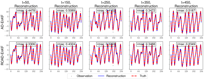
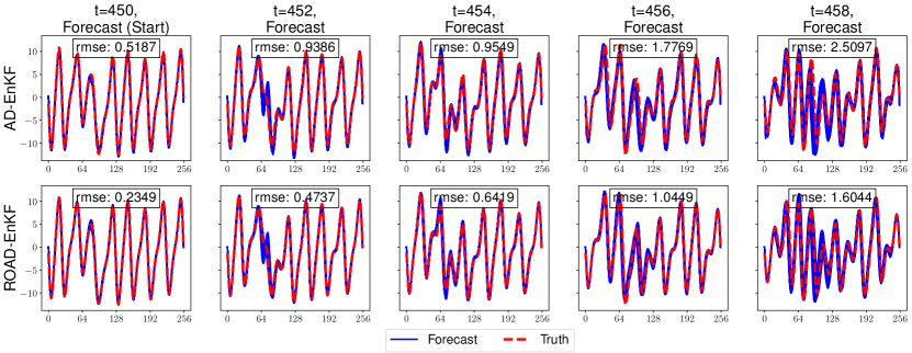
Figure 9: State reconstruction (upper half) and forecast (lower half) performance with partial observation ($d_{u}=256$, $d_{y}=128$) on the KS example in Subsection 5.3. For each method, the reconstructed states $u_{t}$ (blue) for a single test sequence are plotted for $t=50,150,250,350,450$ (column), and the forecasted states (blue) for a single test sequence are plotted for $t=450$ (start of forecast), $452,454,456,458$ (column). The true values of the 256-dimensional states are plotted in red dashed lines, along with the noisy observations in black dots. Both AD-EnKF and ROAD-EnKF perform probabilistic state reconstructions and forecast through particles (all plotted in blue). The reconstruction/forecast RMSEs are computed for each plot.

(a) Ground truth.

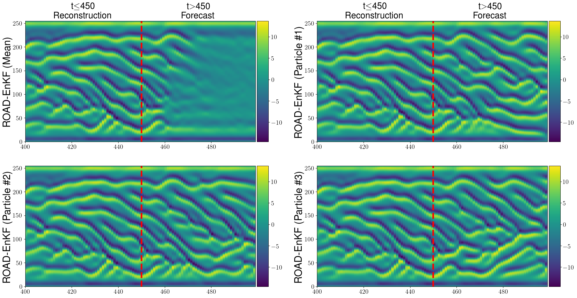
(b) Reconstruction and forecast.

Figure 10: Contour plot of state reconstruction and forecast output of ROAD-EnKF with partial observation ($d_{u}=256$, $d_{y}=128$) on the KS example in Subsection 5.3, as well as the ground truth (top). The particle means of reconstructed and forecasted states for a single test sequence are plotted, for each state dimension (y-axis) and time (x-axis). The reconstructed and forecasted states of three randomly chosen particles are also plotted individually.

6 Conclusions and Future Directions

This paper introduced a computational framework to reconstruct and forecast a partially observed state that evolves according to an unknown or expensive-to-simulate dynamical system. Our ROAD-EnKFs use an EnKF algorithm to estimate by maximum likelihood a surrogate model for the dynamics in a latent space, as well as a decoder from latent space to state space. Our numerical experiments demonstrate the computational advantage of co-learning an inexpensive surrogate model in latent space together with a decoder, rather than a more expensive-to-simulate dynamics in state space.

The proposed computational framework accommodates partial observation of the state, does not require time derivative data, and enables uncertainty quantification. In addition, it provides significant algorithmic flexibility through the choice of latent space, surrogate model for the latent dynamics, and decoder design. In this work, we showed that accurate and cheap reconstructions and forecasts can be obtained by choosing an inexpensive NN surrogate model, and a decoder inspired by recent ideas from operator learning. While adequate choice of NN architecture and decoder may be problem-specific, an important question for further research is to derive guidelines and physics-informed NNs that are well-suited for certain classes of problems.

Appendix A Improving AD-EnKF with Spectral Convolutional Layers

This appendix discusses an enhancement of the AD-EnKF algorithm [20], used for numerical comparisons in Section 5. AD-EnKF runs EnKF on the full-order SSM (2.1)-(2.3) and learns the parameter $\theta=(\alpha^{\top},\beta^{\top})^{\top}$ by auto-differentiating through a similarly defined log-likelihood objective, as in Subsection 3.2. A high dimension of $u$ makes challenging the NN parameterization of $F_{\alpha}$ (resp. $f_{\alpha}$ in the ODE case) in the state dynamics model 2.1. In particular, the local convolutional NN used in [20] does not perform well in the high-dimensional numerical experiments considered in Section 5. We thus propose a more flexible NN parameterization of $F_{\alpha}$ (resp. $f_{\alpha}$) using the idea of spectral convolutional layers.

We design $F_{\alpha}$ (resp. $f_{\alpha}$) in a way similar to the Fourier Neural Decoder, but without the complex linear layer and IDFT step at the beginning. That is, we start with a state variable $u^{\prime}\in\mathbbm{R}^{d_{u}}$ as the input, iteratively apply 4.2 with $v_{0}=u^{\prime}$ to get $v_{L}\in\mathbbm{R}^{n_{L}\times d_{u}}$, followed by a fully-connected network applied over the channel dimension to get the output $u\in\mathbbm{R}^{d_{u}}$. The architecture is the same as Figure 3(a) but we start at $v_{0}$ instead of $z$.

Appendix B Additional Materials: Burgers Example

For SINDy-AE, we use a finite difference approximation computed from data $y_{1:T}$ to approximate the exact time-derivative. The latent space dimension for SINDy-AE is set to 6. Increasing it does not further enhance the performance, but increases the computational cost.

	AD-EnKF (FC, Euler)	AD-EnKF (FC, RK4)	AD-EnKF (Fourier, Euler)	AD-EnKF (Fourier, RK4)	ROAD-EnKF (FC, Euler)	ROAD-EnKF (FC, RK4)
RMSE-r	0.1023	0.0934	0.0537	0.0102	0.0045	0.0044
RMSE-f(30)	0.0999	0.0831	0.1302	0.0212	0.0100	0.0096
RMSE-f(150)	0.1971	0.1608	0.2908	0.0763	0.0664	0.0514
Log-likelihood	$2.31\times 10^{4}$	$2.87\times 10^{4}$	$5.41\times 10^{4}$	$6.40\times 10^{4}$	$6.60\times 10^{4}$	$6.57\times 10^{4}$
Training time (per epoch)	4.97s	5.80s	12.31s	26.75s	11.21s	12.10s
Test time	2.29s	2.97s	4.79s	11.54s	3.28s	4.21s

Table B.1: Ablation study: AD-EnKF versus ROAD-EnKF with different NN parameterization and numerical integration methods for surrogate dynamics (FC: NN with fully-connected layers; Fourier: NN with Fourier layers; Euler: Euler method for ODE integration; RK4: fourth-order Runge Kutta method for ODE integration). Switching from RK4 to Euler method while keeping the same NN configuration gives a computational speed-up, and the speed-up is more noticeable when the NN involves Fourier layers. However, after the switch, the accuracy drops more significantly for AD-EnKF than for ROAD-EnKF. The best configuration for AD-EnKF (Fourier with RK4) still yields a lower accuracy compared to both ROAD-EnKF configurations, while taking more time to compute. (Burgers example, full observation case, Subsection 5.2.)

(a) Ground truth.

Appendix C Additional Materials: Kuramoto-Sivashinky Example

References

- [1] M. Abadi, P. Barham, J. Chen, Z. Chen, A. Davis, J. Dean, M. Devin, S. Ghemawat, G. Irving, M. Isard, et al., Tensorflow: A system for large-scale machine learning, in 12th USENIX Symposium on Operating Systems Design and Implementation (OSDI 16), 2016, pp. 265–283.
- [2] S. Agapiou, O. Papaspiliopoulos, D. Sanz-Alonso, and A. M. Stuart, Importance sampling: Intrinsic dimension and computational cost, Statistical Science, 32 (2017), pp. 405–431.
- [3] Y. Bengio, P. Simard, and P. Frasconi, Learning long-term dependencies with gradient descent is difficult, IEEE Transactions on Neural Networks, 5 (1994), pp. 157–166.
- [4] T. Bengtsson, P. Bickel, B. Li, et al., Curse-of-dimensionality revisited: Collapse of the particle filter in very large scale systems, Probability and statistics: Essays in honor of David A. Freedman, 2 (2008), pp. 316–334.
- [5] P. Benner, S. Gugercin, and K. Willcox, A survey of projection-based model reduction methods for parametric dynamical systems, SIAM Review, 57 (2015), pp. 483–531.
- [6] P. J. Blonigan and Q. Wang, Least squares shadowing sensitivity analysis of a modified Kuramoto–Sivashinsky equation, Chaos, Solitons & Fractals, 64 (2014), pp. 16–25. Nonequilibrium Statistical Mechanics: Fluctuations and Response.
- [7] M. Bocquet, J. Brajard, A. Carrassi, and L. Bertino, Bayesian inference of chaotic dynamics by merging data assimilation, machine learning and expectation-maximization, Foundations of Data Science, 2 (2020), pp. 55–80.
- [8] J. Bradbury, R. Frostig, P. Hawkins, M. J. Johnson, C. Leary, D. Maclaurin, G. Necula, A. Paszke, J. VanderPlas, S. Wanderman-Milne, and Q. Zhang, JAX: composable transformations of Python+NumPy programs, 2018.
- [9] J. Brajard, A. Carrassi, M. Bocquet, and L. Bertino, Combining data assimilation and machine learning to emulate a dynamical model from sparse and noisy observations: A case study with the Lorenz 96 model, Journal of Computational Science, 44 (2020), p. 101171.
- [10] S. L. Brunton, J. L. Proctor, and J. N. Kutz, Discovering governing equations from data by sparse identification of nonlinear dynamical systems, Proceedings of the National Academy of Sciences, 113 (2016), pp. 3932–3937.
- [11] J. Burgers, A mathematical model illustrating the theory of turbulence, vol. 1 of Advances in Applied Mechanics, Elsevier, 1948, pp. 171–199.
- [12] A. Carrassi, M. Bocquet, A. Hannart, and M. Ghil, Estimating model evidence using data assimilation, Quarterly Journal of the Royal Meteorological Society, 143 (2017), pp. 866–880.
- [13] A. Carrassi, M. Ghil, A. Trevisan, and F. Uboldi, Data assimilation as a nonlinear dynamical systems problem: Stability and convergence of the prediction-assimilation system, Chaos: An Interdisciplinary Journal of Nonlinear Science, 18 (2008), p. 023112.
- [14] N. K. Chada, Y. Chen, and D. Sanz-Alonso, Iterative ensemble Kalman methods: A unified perspective with some new variants, Foundations of Data Science, 3 (2021), p. 331.
- [15] N. K. Chada, A. M. Stuart, and X. T. Tong, Tikhonov regularization within ensemble Kalman inversion, SIAM Journal on Numerical Analysis, 58 (2020), pp. 1263–1294.
- [16] K. Champion, B. Lusch, J. N. Kutz, and S. L. Brunton, Data-driven discovery of coordinates and governing equations, Proceedings of the National Academy of Sciences, 116 (2019), pp. 22445–22451.
- [17] N. Chen and A. J. Majda, Conditional Gaussian systems for multiscale nonlinear stochastic systems: prediction, state estimation and uncertainty quantification, Entropy, 20 (2018).
- [18] N. Chen and D. Qi, A physics-informed data-driven algorithm for ensemble forecast of complex turbulent systems, arXiv preprint arXiv:2204.08547, (2022).
- [19] R. T. Q. Chen, Y. Rubanova, J. Bettencourt, and D. K. Duvenaud, Neural ordinary differential equations, in Advances in Neural Information Processing Systems, vol. 31, 2018.
- [20] Y. Chen, D. Sanz-Alonso, and R. Willett, Autodifferentiable ensemble Kalman filters, SIAM Journal on Mathematics of Data Science, 4 (2022), pp. 801–833.
- [21] A. Corenflos, J. Thornton, G. Deligiannidis, and A. Doucet, Differentiable particle filtering via entropy-regularized optimal transport, in International Conference on Machine Learning, PMLR, 2021, pp. 2100–2111.
- [22] E. De Brouwer, J. Simm, A. Arany, and Y. Moreau, GRU-ODE-Bayes: Continuous modeling of sporadically-observed time series, in Advances in Neural Information Processing Systems, vol. 32, 2019.
- [23] A. P. Dempster, N. M. Laird, and D. B. Rubin, Maximum likelihood from incomplete data via the EM algorithm, Journal of the Royal Statistical Society. Series B (Methodological), 39 (1977), pp. 1–38.
- [24] L. Dieci and E. S. Van Vleck, Lyapunov and Sacker–Sell spectral intervals, Journal of Dynamics and Differential Equations, 19 (2007), pp. 265–293.
- [25] L. Dieci and E. S. Van Vleck, Lyapunov exponents: Computation, Encyclopedia of Applied and Computational Mathematics, (2015), pp. 834–838.
- [26] A. Doucet and A. M. Johansen, A tutorial on particle filtering and smoothing: Fifteen years later, Handbook of Nonlinear Filtering, 12 (2009), p. 3.
- [27] D. Dreano, P. Tandeo, M. Pulido, B. Ait-El-Fquih, T. Chonavel, and I. Hoteit, Estimating model-error covariances in nonlinear state-space models using Kalman smoothing and the expectation–maximization algorithm, Quarterly Journal of the Royal Meteorological Society, 143 (2017), pp. 1877–1885.
- [28] C. Drovandi, R. G. Everitt, A. Golightly, and D. Prangle, Ensemble MCMC: accelerating pseudo-marginal MCMC for state space models using the ensemble Kalman filter, Bayesian Analysis, 17 (2022), pp. 223–260.
- [29] G. Evensen, Sequential data assimilation with a nonlinear quasi-geostrophic model using Monte Carlo methods to forecast error statistics, Journal of Geophysical Research: Oceans, 99 (1994), pp. 10143–10162.
- [30] G. Evensen, Data Assimilation: the Ensemble Kalman Filter, Springer Science & Business Media, 2009.
- [31] A. Farchi, P. Laloyaux, M. Bonavita, and M. Bocquet, Using machine learning to correct model error in data assimilation and forecast applications, Quarterly Journal of the Royal Meteorological Society, 147 (2021), pp. 3067–3084.
- [32] O. A. Ghattas and D. Sanz-Alonso, Non-asymptotic analysis of ensemble kalman updates: Effective dimension and localization, arXiv preprint arXiv:2208.03246, (2022).
- [33] M. B. Giles, Collected matrix derivative results for forward and reverse mode algorithmic differentiation, in Advances in Automatic Differentiation, Springer, 2008, pp. 35–44.
- [34] F. J. Gonzalez and M. Balajewicz, Deep Convolutional Recurrent Autoencoders for Learning Low-dimensional Feature Dynamics of Fluid Systems, arXiv preprint arXiv:1808.01346, (2018).
- [35] N. J. Gordon, D. J. Salmond, and A. F. Smith, Novel approach to nonlinear/non-Gaussian Bayesian state estimation, IEE proceedings F (radar and signal processing), 140 (1993), pp. 107–113.
- [36] J. Guibas, M. Mardani, Z. Li, A. Tao, A. Anandkumar, and B. Catanzaro, Efficient token mixing for transformers via adaptive Fourier neural operators, in International Conference on Learning Representations, 2021.
- [37] P. A. Guth, C. Schillings, and S. Weissmann, Ensemble Kalman filter for neural network-based one-shot inversion, Optimization and Control for Partial Differential Equations: Uncertainty Quantification, Open and Closed-Loop Control, and Shape Optimization, 29 (2022), p. 393.
- [38] T. M. Hamill, J. S. Whitaker, and C. Snyder, Distance-dependent filtering of background error covariance estimates in an ensemble Kalman filter, Monthly Weather Review, 129 (2001), pp. 2776–2790.
- [39] J. Harlim, S. W. Jiang, S. Liang, and H. Yang, Machine learning for prediction with missing dynamics, Journal of Computational Physics, 428 (2021), p. 109922.
- [40] Y. He, S.-H. Kang, W. Liao, H. Liu, and Y. Liu, Robust identification of differential equations by numerical techniques from a single set of noisy observation, SIAM Journal on Scientific Computing, 44 (2022), pp. A1145–A1175.
- [41] Y. He, N. Suh, X. Huo, S. H. Kang, and Y. Mei, Asymptotic theory of regularized PDE identification from a single noisy trajectory, SIAM/ASA Journal on Uncertainty Quantification, 10 (2022), pp. 1012–1036.
- [42] Y. He, H. Zhao, and Y. Zhong, How much can one learn a partial differential equation from its solution?, arXiv preprint arXiv:2204.04602, (2022).
- [43] P. L. Houtekamer and H. L. Mitchell, A sequential ensemble Kalman filter for atmospheric data assimilation, Monthly Weather Review, 129 (2001), pp. 123–137.
- [44] P. L. Houtekamer and F. Zhang, Review of the ensemble Kalman filter for atmospheric data assimilation, Monthly Weather Review, 144 (2016), pp. 4489–4532.
- [45] I. D. Jordan, P. A. Sokół, and I. M. Park, Gated recurrent units viewed through the lens of continuous time dynamical systems, Frontiers in Computational Neuroscience, 15 (2021).
- [46] R. E. Kalman, A new approach to linear filtering and prediction problems, Journal of Basic Engineering, 82 (1960), pp. 35–45.
- [47] M. Katzfuss, J. R. Stroud, and C. K. Wikle, Understanding the ensemble Kalman filter, The American Statistician, 70 (2016), pp. 350–357.
- [48] P. Kidger, J. Morrill, J. Foster, and T. Lyons, Neural controlled differential equations for irregular time series, Advances in Neural Information Processing Systems, (2020).
- [49] D. P. Kingma and M. Welling, Auto-Encoding Variational Bayes, in 2nd International Conference on Learning Representations, 2014.
- [50] Y. Kuramoto and T. Tsuzuki, Persistent propagation of concentration waves in dissipative media far from thermal equilibrium, Progress of Theoretical Physics, 55 (1976), pp. 356–369.
- [51] K. J. Law, D. Sanz-Alonso, A. Shukla, and A. M. Stuart, Filter accuracy for the Lorenz 96 model: Fixed versus adaptive observation operators, Physica D: Nonlinear Phenomena, 325 (2016), pp. 1–13.
- [52] T. A. Le, M. Igl, T. Rainforth, T. Jin, and F. Wood, Auto-encoding sequential Monte Carlo, arXiv preprint arXiv:1705.10306, (2017).
- [53] F. Le Gland and L. Mevel, Recursive identification in hidden Markov models, in Proceedings of the 36th Conference on Decision and Control, vol. 4, 1997, pp. 3468–3473.
- [54] M. Lechner and R. Hasani, Learning long-term dependencies in irregularly-sampled time series, arXiv preprint arXiv:2006.04418, (2020).
- [55] M. Levine and A. Stuart, A framework for machine learning of model error in dynamical systems, Communications of the American Mathematical Society, 2 (2022), pp. 283–344.
- [56] Z. Li, N. Kovachki, K. Azizzadenesheli, B. Liu, K. Bhattacharya, A. Stuart, and A. Anandkumar, Fourier neural operator for parametric partial differential equations, in International Conference on Learning Representations, 2020.
- [57] Z. C. Lipton, J. Berkowitz, and C. Elkan, A critical review of recurrent neural networks for sequence learning, arXiv preprint arXiv:1506.00019, (2015).
- [58] B. Lusch, J. N. Kutz, and S. L. Brunton, Deep learning for universal linear embeddings of nonlinear dynamics, Nature Communications, 9 (2018), pp. 1–10.
- [59] J. Maclean and E. S. Van Vleck, Particle filters for data assimilation based on reduced-order data models, Quarterly Journal of the Royal Meteorological Society, 147 (2021), pp. 1892–1907.
- [60] C. J. Maddison, J. Lawson, G. Tucker, N. Heess, M. Norouzi, A. Mnih, A. Doucet, and Y. Teh, Filtering variational objectives, Advances in Neural Information Processing Systems, 30 (2017).
- [61] A. J. Majda and D. Qi, Strategies for reduced-order models for predicting the statistical responses and uncertainty quantification in complex turbulent dynamical systems, SIAM Review, 60 (2018), pp. 491–549.
- [62] X. Mao, C. Shen, and Y.-B. Yang, Image restoration using very deep convolutional encoder-decoder networks with symmetric skip connections, Advances in Neural Information Processing Systems, 29 (2016).
- [63] R. Maulik, B. Lusch, and P. Balaprakash, Reduced-order modeling of advection-dominated systems with recurrent neural networks and convolutional autoencoders, Physics of Fluids, 33 (2021), p. 037106.
- [64] S. Metref, A. Hannart, J. Ruiz, M. Bocquet, A. Carrassi, and M. Ghil, Estimating model evidence using ensemble-based data assimilation with localization–The model selection problem, Quarterly Journal of the Royal Meteorological Society, 145 (2019), pp. 1571–1588.
- [65] C. Naesseth, S. Linderman, R. Ranganath, and D. Blei, Variational sequential Monte Carlo, in International Conference on Artificial Intelligence and Statistics, PMLR, 2018, pp. 968–977.
- [66] D. Nguyen, S. Ouala, L. Drumetz, and R. Fablet, Em-like learning chaotic dynamics from noisy and partial observations, arXiv preprint arXiv:1903.10335, (2019).
- [67] L. Palatella, A. Carrassi, and A. Trevisan, Lyapunov vectors and assimilation in the unstable subspace: theory and applications, Journal of Physics A: Mathematical and Theoretical, 46 (2013), p. 254020.
- [68] O. Papaspiliopoulos and M. Ruggiero, Optimal filtering and the dual process, Bernoulli, 20 (2014), pp. 1999–2019.
- [69] A. Paszke, S. Gross, F. Massa, A. Lerer, J. Bradbury, G. Chanan, T. Killeen, Z. Lin, N. Gimelshein, L. Antiga, A. Desmaison, A. Kopf, E. Yang, Z. DeVito, M. Raison, A. Tejani, S. Chilamkurthy, B. Steiner, L. Fang, J. Bai, and S. Chintala, Pytorch: An imperative style, high-performance deep learning library, in Advances in Neural Information Processing Systems 32, H. Wallach, H. Larochelle, A. Beygelzimer, F. d'Alché-Buc, E. Fox, and R. Garnett, eds., Curran Associates, Inc., 2019, pp. 8024–8035.
- [70] M. Pulido, P. Tandeo, M. Bocquet, A. Carrassi, and M. Lucini, Stochastic parameterization identification using ensemble Kalman filtering combined with maximum likelihood methods, Tellus A: Dynamic Meteorology and Oceanography, 70 (2018), pp. 1–17.
- [71] D. J. Rezende, S. Mohamed, and D. Wierstra, Stochastic backpropagation and approximate inference in deep generative models, in International Conference on Machine Learning, PMLR, 2014, pp. 1278–1286.
- [72] M. Roth, G. Hendeby, C. Fritsche, and F. Gustafsson, The Ensemble Kalman filter: a signal processing perspective, EURASIP Journal on Advances in Signal Processing, 2017 (2017), pp. 1–16.
- [73] Y. Rubanova, R. T. Q. Chen, and D. K. Duvenaud, Latent ordinary differential equations for irregularly-sampled time series, in Advances in Neural Information Processing Systems, vol. 32, 2019.
- [74] D. Sanz-Alonso and A. M. Stuart, Long-time asymptotics of the filtering distribution for partially observed chaotic dynamical systems, SIAM/ASA Journal on Uncertainty Quantification, 3 (2015), pp. 1200–1220.
- [75] D. Sanz-Alonso, A. M. Stuart, and A. Taeb, Inverse Problems and Data Assimilation, arXiv preprint arXiv:1810.06191, (2019).
- [76] H. Schaeffer, G. Tran, and R. Ward, Extracting sparse high-dimensional dynamics from limited data, SIAM Journal on Applied Mathematics, 78 (2018), pp. 3279–3295.
- [77] G. Sivashinsky, Nonlinear analysis of hydrodynamic instability in laminar flames—i. derivation of basic equations, Acta Astronautica, 4 (1977), pp. 1177–1206.
- [78] A. Spantini, D. Bigoni, and Y. Marzouk, Inference via low-dimensional couplings, The Journal of Machine Learning Research, 19 (2018), pp. 2639–2709.
- [79] J. R. Stroud and T. Bengtsson, Sequential state and variance estimation within the ensemble Kalman filter, Monthly Weather Review, 135 (2007), pp. 3194–3208.
- [80] J. R. Stroud, M. Katzfuss, and C. K. Wikle, A Bayesian adaptive ensemble Kalman filter for sequential state and parameter estimation, Monthly Weather Review, 146 (2018), pp. 373–386.
- [81] J. R. Stroud, M. L. Stein, B. M. Lesht, D. J. Schwab, and D. Beletsky, An ensemble Kalman filter and smoother for satellite data assimilation, Journal of the American Statistical Association, 105 (2010), pp. 978–990.
- [82] I. Sutskever, O. Vinyals, and Q. V. Le, Sequence to sequence learning with neural networks, in Advances in Neural Information Processing Systems, vol. 27, 2014.
- [83] I. Szunyogh, E. J. Kostelich, G. Gyarmati, E. Kalnay, B. R. Hunt, E. Ott, E. Satterfield, and J. A. Yorke, A local ensemble transform Kalman filter data assimilation system for the NCEP global model, Tellus A: Dynamic Meteorology and Oceanography, 60 (2008), pp. 113–130.
- [84] P. Tandeo, M. Pulido, and F. Lott, Offline parameter estimation using EnKF and maximum likelihood error covariance estimates: Application to a subgrid-scale orography parametrization, Quarterly Journal of the Royal Meteorological Society, 141 (2015), pp. 383–395.
- [85] M. K. Tippett, J. L. Anderson, C. H. Bishop, T. M. Hamill, and J. S. Whitaker, Ensemble square root filters, Monthly Weather Review, 131 (2003), pp. 1485–1490.
- [86] G. Tran and R. Ward, Exact recovery of chaotic systems from highly corrupted data, Multiscale Modeling & Simulation, 15 (2017), pp. 1108–1129.
- [87] A. Trevisan, M. D’Isidoro, and O. Talagrand, Four-dimensional variational assimilation in the unstable subspace and the optimal subspace dimension, Quarterly Journal of the Royal Meteorological Society, 136 (2010), pp. 487–496.
- [88] G. Ueno and N. Nakamura, Iterative algorithm for maximum-likelihood estimation of the observation-error covariance matrix for ensemble-based filters, Quarterly Journal of the Royal Meteorological Society, 140 (2014), pp. 295–315.
- [89] Z. Y. Wan and T. P. Sapsis, Reduced-space Gaussian Process Regression for data-driven probabilistic forecast of chaotic dynamical systems, Physica D: Nonlinear Phenomena, 345 (2017), pp. 40–55.
- [90] G. C. Wei and M. A. Tanner, A Monte Carlo implementation of the EM algorithm and the poor man’s data augmentation algorithms, Journal of the American Statistical Association, 85 (1990), pp. 699–704.
- [91] J. S. Whitaker, T. M. Hamill, X. Wei, Y. Song, and Z. Toth, Ensemble data assimilation with the NCEP Global Forecast System , Monthly Weather Review, 136 (2008), pp. 463–482.
- [92] A. Wikner, J. Pathak, B. Hunt, M. Girvan, T. Arcomano, I. Szunyogh, A. Pomerance, and E. Ott, Combining machine learning with knowledge-based modeling for scalable forecasting and subgrid-scale closure of large, complex, spatiotemporal systems, Chaos: An Interdisciplinary Journal of Nonlinear Science, 30 (2020), p. 053111.
- [93] R. J. Williams and D. Zipser, Gradient-based learning algorithms for recurrent, Backpropagation: Theory, Architectures, and Applications, 433 (1995), p. 17.
- [94] M. A. Woodbury, Inverting Modified Matrices, Statistical Research Group, 1950.
- [95] L. M. Yang and I. Grooms, Machine learning techniques to construct patched analog ensembles for data assimilation, Journal of Computational Physics, 443 (2021), p. 110532.
- [96] Y. Yu, X. Si, C. Hu, and J. Zhang, A Review of Recurrent Neural Networks: LSTM Cells and Network Architectures, Neural Computation, 31 (2019), pp. 1235–1270.