A first detection of neutral hydrogen intensity mapping on Mpc scales at $z\approx 0.32$ and $z\approx 0.44$

Abstract

We report the first direct detection of the cosmological power spectrum using the intensity signal from 21-cm emission of neutral hydrogen (HI), derived from interferometric observations with the L-band receivers of the new MeerKAT radio telescope. Intensity mapping is a promising technique to map the three-dimensional matter distribution of the Universe at radio frequencies and probe the underlying Cosmology. So far, detections have only been achieved through cross-correlations with galaxy surveys. Here we present independent measurements of the HI power spectrum at redshifts $0.32$ and $0.44$ with high statistical significance using a foreground avoidance method (at $8.0\sigma$ and $11.5\sigma$ respectively). We constrain the rms of the fluctuations of the HI distribution to be $\sigma_{\rm HI}=(0.44\pm 0.04)\,{\rm mK}$ and $\sigma_{\rm HI}=(0.63\pm 0.03)\,{\rm mK}$ respectively at scales of 1.0 Mpc. The information contained in the power spectrum measurements allows us to probe the parameters of the HI mass function and HI halo model. These results are a significant step towards precision cosmology with HI intensity mapping using the new generation of radio telescopes.

tablenum SIXtablenum

1 Introduction

The 21-cm hyperfine transition of neutral hydrogen (HI) is a prime tracer of the HI gas in galaxies as well as the inter-galactic medium at high redshifts. Observations at the radio frequencies of this line (at or below $1420$ MHz) are free from dust absorption and have high redshift resolutions due to standard digital processing techniques from radio telescopes. Given the abundance of HI gas in the Universe, observations with the 21-cm line can be a powerful probe of the structure and evolution of the Universe. However, the inherent weakness of the 21-cm signal has restricted HI galaxy surveys to the nearby Universe (redshifts $\lesssim 0.1$; e.g. Jones et al. (2018)). The upcoming generation of radio telescopes will push this to higher redshifts but only over small areas and large HI masses (Maddox et al., 2021). The intensity mapping (IM) technique circumvents this sensitivity issue by averaging over the collective emission from many unresolved galaxies and producing low angular resolution maps of the HI intensity (albeit still with redshift resolutions comparable to galaxy spectroscopic surveys). The possibilities opened by this new observational window promise a breakthrough in constraining cosmological theories in the very near future (Bharadwaj & Sethi, 2001; Battye et al., 2004; Morales & Wyithe, 2010; Bull et al., 2015). However, the continuous mapping of the skies requires separating the 21-cm line from other signals at a given frequency. This is particularly challenging due to the presence of strong radio foregrounds (Wolz et al., 2014; Olivari et al., 2016; Cunnington et al., 2019; Liu & Shaw, 2020). So far, measurements have been hampered by the extraordinary calibration challenges and detections have only been achieved through cross-correlations with galaxy surveys since the systematics in the HI maps are not expected to correlate with data at other wavelengths. The first cross-correlation detection was obtained with the single-dish Green Bank Telescope (GBT)(Chang et al., 2010; Masui et al., 2013; Wolz et al., 2022), followed by measurements with the Parkes telescope (Anderson et al., 2018). More recently, the CHIME interferometer made a stacking detection using this technique over a wide area (CHIME Collaboration et al., 2022) (but see also Chowdhury et al. (2020)).

The recently built MeerKAT 64-dish telescope array in South Africa has also been proposed as an exquisite survey machine for HI IM (Santos et al., 2017) and acts as a precursor for the upcoming SKA Observatory (Santos et al., 2015; Square Kilometre Array Cosmology Science Working Group et al., 2020). For IM surveys, the array is used in single dish mode in order to access the large cosmological scales and pilot tests have been underway (Wang et al., 2021). A detection of the HI power spectrum in cross-correlation with galaxies from the WiggleZ Dark Energy Survey has been made (Cunnington et al., 2023). However, the large primary beam limits the minimum accessible scales to tens of Mpc and interferometric IM observations can provide crucial information on smaller scales and the nonlinear regime.The core heavy dish distribution of the MeerKAT interferometer can measure scales up to $60$ Mpc at $z<0.65$ in the $L$-band frequency range (856 MHz $<\nu<$ 1712 MHz) and up to $165$ Mpc at $z<1.4$ in the $UHF$-band (580 MHz $<\nu<$ 1015 MHz). Forecasts in Paul et al. (2021) predict that a statistical detection of the HI IM power spectrum is possible with $\sim 100$ hrs of observation with MeerKAT. Using surveys such as the MeerKAT International GHz Tiered Extragalactic Exploration (MIGHTEE) Survey (Taylor & Jarvis, 2017), we can detect the HI power spectrum in narrow redshift bins across a range of redshifts, opening up a new window for probing the astrophysics of the HI galaxies (Chen et al., 2021).

In this work, we report the first detection of the HI intensity auto-power spectrum in the interferometric IM mode at frequencies of $986$ MHz ($z\approx 0.44$) and $1077.5$ MHz ($z\approx 0.32$) by analysing $\sim 96$ hrs of MeerKAT data. Observations were carried out with the $L$-band configuration and 4,000 frequency channels with a resolution of $209$ KHz, during the commissioning process of MeerKAT in 2018. The total 96 hrs of data spanned through 9 separate observing sessions all targeted one single pointing corresponding to a sky area of $\sim 2$ deg² at 1.0 GHz. The J2000 center position of this field at $\alpha=04^{\rm{h}}13^{\rm{m}}26.4^{\rm{s}},\delta=$$$ in the Southern Hemisphere was specifically selected to minimize artifacts caused by bright sources, making it a prime candidate for the IM technique. We processed the raw data from scratch, flagging radio frequency interference (RFI) and doing full polarization calibration using the processMeerKAT (Collier et al., 2021) software pipeline. We then focused our analysis on two RFI free frequency ranges centered at $986$ and $1077.5$ MHz with 220 frequency channels each, equalling a frequency width of $\approx 46$ MHz. The smaller bandwidth segments are chosen to minimize the effects of cosmological evolution ($\Delta z\sim 0.06$).

2 Detection methodology

In this section we present the formalism to compute the HI power spectrum, which acts as a probe of the underlying dark matter distribution and the biased relation to the HI. We estimate the power spectrum using the ‘delay spectrum’ approach (Morales & Hewitt, 2004; McQuinn et al., 2006; Parsons et al., 2012, 2014; Paul et al., 2016) with our custom-built pipeline (Paul et al., 2021): instead of producing images and HI cubes, we work directly with the interferometer visibilities, $V(\bm{b},t,\nu)$, which records the spatial correlation of the electric field for each antenna-pair (denoted by the baseline vector $\bm{b}$). In the limit of small sky areas, $V(\bm{b},t,\nu)$ measures the 2-d Fourier transform of the sky at each frequency $\nu$ and time $t$. The “angular” Fourier mode is related to the baseline vector by $\bm{k_{\perp}}=\frac{2\pi\bm{b}}{\lambda x}$, where $\nu_{21}$ is the rest frame frequency of the 21-cm line, $H(z)$ is the Hubble parameter at redshift $z$ ($1+z=\nu_{21}/\nu$) and $x$ is the comoving distance to that redshift. Since we are observing the same sky patch, visibilities at a given frequency with the same $\bm{k_{\perp}}$ should have the same value at any given time (except for noise and RFI). We, therefore, average them in a 2-d $\bm{k_{\perp}}$ grid, with a bin width chosen to avoid decorrelation given the primary beam size. The primary beam convolves with the sky signal in Fourier space, mixing different $k_{\perp}$-modes. In order to minimise the effects of mode-mixing by the primary beam, we choose a large grid size, $\Delta u=60\lambda$, corresponding to $\Delta k_{\perp}\sim 0.3\,{\rm Mpc^{-1}}$, so that the width of the primary beam in $k_{\perp}$-space is negligible. This bin size is kept constant across the frequency since, as mentioned above, the redshift evolution within each of the small bands analyzed is negligible. Finally, we Fourier transform the visibilities along the frequency axis (called the delay transform), resulting in the delay-space ($\tau$) visibility function $\tilde{V}(\bm{k_{\perp}},\tau)$. In the limit of small bandwidths, this delay-space can be related to the line of sight Fourier mode, $k_{\parallel}$, through $k_{\parallel}=\frac{2\pi\tau\nu_{21}H(z)}{c(1+z)^{2}}$. This creates the 3-d Fourier cube $\bm{k}=(\bm{k_{\perp}},k_{\parallel})$ and the 3-d power spectrum (‘delay spectrum’– Morales & Hewitt, 2004; McQuinn et al., 2006; Parsons et al., 2012, 2014; Paul et al., 2016):

$$P_{\rm{D}}(\bm{k_{\perp}},k_{\parallel})\equiv\frac{x^{2}y}{\Omega_{\rm ps}B}\left(\frac{\lambda^{2}}{2k_{B}}\right)^{2}{\rm Re}\{\tilde{V}_{1}(\bm{b},\tau)\tilde{V}_{2}^{*}(\bm{b},\tau)\},$$ (1)

with $\lambda$ denoting the wavelength at the band-center, $k_{B}$ the Boltzmann constant and $y$ the comoving depth corresponding to the bandwidth $B$; the visibility functions $\tilde{V}_{1}$ and $\tilde{V}_{2}$ correspond to different times and we are taking the real part (${\rm Re}\{\}$) of the product (such cross product will remove the noise bias on average). $\Omega_{\rm ps}$ denotes the power-squared primary beam area, i.e. the solid angle integral of the primary beam squared (Santos et al., 2005; Parsons et al., 2014),

$$\Omega_{\rm ps}=\int{\rm d}l\,{\rm d}m\,A^{2}(l,m),$$ (2)

where $A(l,m)$ is the primary beam attenuation. The power-squared primary beam area is calculated using the eidos MeerKAT beam model (Asad et al., 2021).

2.1 Cosmological parameters

We use the flat $\Lambda$CDM cosmological parameters $[\Omega_{m},\Omega_{b},h,n_{s},\sigma_{8}]=[0.311,0.049,0.677,0.967,0.8102]$ from Planck 2018 results (Planck Collaboration et al., 2018) throughout this work.

2.2 MeerKAT observations

Situated in the Karoo region in South Africa, the MeerKAT telescope consists of 64 dish antennas of $13.5$ m diameter. The telescope array has a dense core of $48$ antennas placed within a $1$ km diameter, and another $16$ antennas are mounted at larger distances up to a 4 km radius from the center. This array layout leads to a high number of short baselines which leads to higher sensitivity at low $\bm{k_{\perp}}$, i.e. the larger cosmological scales.

The observed field J2000, located at $\alpha=04^{\rm{h}}13^{\rm{m}}26.4^{\rm{s}},\delta=$$$, contains a limited amount of bright radio foreground sources. It was previously studied to produce the deepest radio source count to date using the P(D) technique, revealing the bulk of the star formation history of the universe (Mauch et al., 2020) and therefore has been chosen for the analysis presented in this paper. The observations were carried out with the $L$-band configuration and the data used in this work is a subset of the publicly available data observed under the Proposal ID: SCI-20180426-TM-01 (Mauch et al., 2020). The total 96 hrs of data spanned through 9 separate observing sessions and all of them utilize at least 58 antennas. Each scan on the target field lasted for 15 minutes followed by a 2 minutes observation of the secondary (e.g. phase) calibrator $\rm{PKS}\,\rm{J}0252{\text{-}}7104$. The primary flux and bandpass calibrator $\rm{PKS}\,\rm{B}1934{\text{-}}638$ was observed for 10 minutes at the beginning of each session and after that, in regular intervals of 3 hours. The flagging of unwanted radio frequency interference (RFI) from terrestrial sources and subsequent calibration of the uncalibrated data were performed with the processMeerKAT (Collier et al., 2021) software which is built for calibrating MeerKAT interferometer data. The processMeerKAT uses Common Astronomy Software Applications (CASA, McMullin et al. 2007) package routines for RFI removal, calculations of phase and flux gains from the reference calibrator observations. In particular, it uses $\rm{PKS}\,\rm{B}1934{\text{-}}638$ to estimate the delay and bandpass solutions which are applied on $\rm{PKS}\,\rm{J}0252{\text{-}}7104$ data to calculate the time-dependent complex gains. The final gain corrections are applied to the target data to perform a full-polarization calibration. Following this, we perform three rounds of phase only self-calibration to 1 of the 9 observing sessions datasets with a solution interval of $60$s. The final resulting model is then used as the initial model to perform phase self-calibration to the rest of the 8 datasets. As the target field does not contain any dominant point sources, we do not perform any amplitude self-calibration. We report that, for each observing sessions, the signal-to-noise ratio of the gain solutions is $\sim 10^{3}$. Assuming that the calibration errors scale down as we average over all observing sessions, the overall calibration error is $10^{-5}$, sufficient for containing foreground leakage (Barry et al., 2016). After flagging the undesired data and performing the calibration steps, the data were split to a $952{\text{-}}1170$ MHz sub-band and $8$s time integration. For computing the delay power spectrum, we adopt a visibility-based approach as described in the previous section. Therefore, no image cubes are used in our analysis pipeline. Moreover, our pipeline relies on foreground isolation and thus identifying individual foreground sources in the map domain is not required. However, for demonstration purposes, we present a frequency-averaged Stokes I image of the field at $1077.5$ MHz from a single dataset of $12.75$ hrs tracking using the subband $952-1170$ MHz in Figure 1. As shown, the flux scale for the continuum foreground emission of the DEEP2 field is below 0.1mJy/beam, ideal for detecting the faint HI signal.

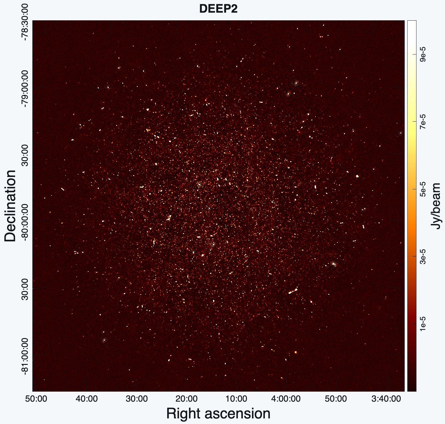
Figure 1: Stokes I frequency-averaged image of the field at $1077.5$ MHz from 1 ($12.75$ hrs tracking) out of 9 datasets. (Image rendered with CARTA (Comrie et al., 2021))

2.3 Power spectrum estimation

To calculate the power spectrum, we further split the visibility datasets into two smaller bands of $\approx 46$ MHz width centered at $986$ and $1077.5$ MHz respectively. The smaller bandwidth segments are chosen to minimize the effects of cosmological evolution. We compute the power spectrum for these two cases separately.

In a tracking observation, each baseline refers to a particular $(u,v)$ point on the $uv$ plane at a given time. The $(u,v)$ coordinate changes to a new value at every integration interval. We generate visibility cubes in the baseline ($uv$)-frequency ($\nu$) domain by gridding the $uv$ plane into discrete cells of size $\Delta u=\Delta v=60\lambda$. The $(u,v)$ coordinates are calculated at the band center. In each observing session, we split the baselines based on the parity of the scan id they belong to. We construct the “even scan” and “odd scan” visibility gridded cubes from the 9 observing sessions, excluding the flagged baselines. We only consider $uv$ points for which the visibility data has at least $80$ percent unflagged channels to mitigate potential weak wide-band RFI. Moreover, the flagged channels (if any) are substituted with the nearest neighbour unflagged channel data. This ensures even sampling across channels when we perform the Fast Fourier Transform (FFT) during the delay transformation. We checked that the results from unsubstituted gridded visibility are consistent with the nearest neighbour substituted data. Assuming the sky signal to be the same within a $uv$ pixel, all visibility data within it are then averaged. Following this, we apply an FFT along the frequency axis for every $uv$ pixel, producing two $u$-$v$-delay ($\tau$) cubes. During this delay transformation, the averaged visibility data is multiplied with the Blackman-Harris spectral window function that suppresses the foreground power leakage to higher $k_{\parallel}$ modes. Next, we cross-correlate between different cubes, computing the cylindrical $(\bm{k_{\perp}},k_{\parallel})$ power spectrum using Equation 1. This cross-correlation removes the noise bias in our calculation, and it is also useful to minimize any time-dependent systematics present in the data.

In the case of statistical isotropy and homogeneity, the power spectrum should be only a function of $k=\sqrt{k_{\perp}^{2}+k_{\parallel}^{2}}$. However, the instrumental noise contribution evolves as a function of $k_{\perp}$ due to the baseline distribution of the array. In our analysis, since we split the dataset into two time blocks and cross-correlate the visibilities, the noise should decorrelate between different times and therefore noise bias correction is not needed. The isotropy is also broken due to HI redshift space distortions, which at these small scales tend to reduce the amplitude of fluctuations for large $k_{\parallel}$ along the line of sight. Nevertheless, the attenuation along the line of sight for the HI signal is much weaker than the attenuation for the foregrounds. The foregrounds such as the Galactic synchrotron emission and radio galaxies are smooth in frequency and contribute power at short delays (small $k_{\parallel}$). This allows us to isolate the contaminants from the HI signal by using the foreground avoidance technique (Datta et al., 2010; Morales et al., 2012; Parsons et al., 2012; Vedantham et al., 2012; Pober et al., 2013; Paul et al., 2016; Chen et al., 2023).

Here, we employ a conservative approach to compute the 1-d power spectrum and only include those $(\bm{k_{\perp}},k_{\parallel})$ pixels which are way above the horizon limit of the foreground wedge. The horizon limit is defined as (Liu et al., 2014)

$$k_{\parallel}=\frac{xH_{0}E(z)\sin\theta_{0}}{c(1+z)}k_{\perp},$$ (3)

where $\theta_{0}$ is the angular extent of the MeerKAT dishes. Due to the small field-of-view and small sidelobes of the MeerKAT telescope, the horizon limit is close to $k_{\parallel}\sim 0.02k_{\perp}$. However, it does not exclude modes that are susceptible to foreground leakage from the sidelobes and instrument systematics. Assuming the most extreme case that leakage of bright foreground sources from the side lobes extends to the entire sky, i.e. $\sin\theta_{0}=1$, the horizon limit becomes $k_{\parallel}\sim 0.26k_{\perp}$. Therefore, we use a much stricter selection criterion $k_{\parallel}=0.3k_{\perp}$ to ensure the robustness of our results.

Apart from the foreground avoidance, we also use thermal noise simulations to flag outliers of the delay powers in $k$-space to mitigation residual systematics, which we discuss in details in Appendix A. To estimate the instrument noise contribution in the power spectrum variance, we generate a cylindrical thermal noise power spectrum where each calibrated visibility component is replaced with a simulated thermal noise visibility generated from a zero mean random process with standard deviation (Taylor et al., 1999)

$$\sigma_{\rm{N}}=\frac{2k_{\rm{B}}T_{\rm{sys}}}{A_{e}\sqrt{\delta\nu\delta t}}$$ (4)

where $T_{\rm{sys}}$ and $A_{e}$ are the system temperature and effective area of each antenna respectively, $k_{\rm{B}}$ is the Boltzmann constant, $\delta\nu=208.984$ kHz is the channel width and $\delta t=8$s is the time resolution. The thermal noise amplitude depends on the natural sensitivity of the instrument $A_{e}/T_{\rm sys}$. We estimate the natural sensitivity at each frequency sub-band by calculating the variance of the Stokes V visibility data (see Appendix A for more details). We find $A_{e}/T_{\rm sys}=6.65\,{\rm m^{2}/K}$ for $z=0.32$ and $6.48\,{\rm m^{2}/K}$ for $z=0.44$, consistent with the anticipated performance $A_{e}/T_{\rm sys}=6.22\,{\rm m^{2}/K}$. We then generate $10000$ realizations of the noise power spectrum given the natural sensitivity $A_{e}/T_{\rm sys}$ to verify our calculations. The Stokes V estimate and the simulation outcome are presented in Figure 9 in Appendix A. We then assign the variance of the thermal noise power across the 10000 realisations at each $k-$pixel $\sigma^{2}(\bm{k_{\perp}},k_{\parallel})$ as the variance of the delay power spectrum. For a given $\bm{k_{\perp}}$, $\sigma$ is approximately constant across $k_{\parallel}$, only changing across $\bm{k_{\perp}}$ depending on the baseline density. At this stage, we flag $\bm{k}$ pixels for which $|P(\bm{k_{\perp}},k_{\parallel})-P_{\rm TN}(\bm{k_{\perp}},k_{\parallel})|>5\sigma(\bm{k_{\perp}},k_{\parallel})$ to exclude $k$-modes affected by any residual systematics. Note that the thermal noise simulations are performed for each gridded visibility data set separately, since different timeblocks and Stokes parameters at different frequency sub-bands have different $u$-$v$ sampling. The $5-\sigma$ flagging is done in the 3-d auto-power of the Stokes I visibility for each timeblock at each sub-band individually. If the 3-d $k$-pixel is flagged in either even or odd scans, it is excluded from the power spectrum estimation in the cross-power. We have verified that this selection criteria results in negligible signal loss with our simulations.

From the 3-d cylindrical power spectrum $P(\bm{k_{\perp}},k_{\parallel})$, we use inverse noise variance weighting ($1/\sigma^{2}(\bm{k_{\perp}},k_{\parallel})$) to calculate the optimal 2-d power spectrum $P(k_{\perp},k_{\parallel})$ with $k_{\perp}=|\bm{k_{\perp}}|$ and 1-d power spectrum $P(k)$ with $k=|(\bm{k_{\perp}},k_{\parallel})|$.

$$\hat{P}_{\rm D}^{i}=\big{(}\sum_{j}P_{\rm D}^{j}w_{j}\big{)}/\big{(}\sum_{j}w_{j}\big{)},$$ (5)

where $j$ loops over all the $k$-points that fall into the $i^{\rm th}$ $k$-bin and $w_{j}=1/\sigma^{2}_{j}$ is the inverse covariance weight calculated from the thermal noise simulations mentioned above. The errors are calculated from the sampling variance of the 3-D powers in each bin

$$(\Delta P_{\rm D}^{\rm i})^{2}=\big{(}\sum_{j}(P_{\rm D}^{\rm j}-\hat{P}_{\rm D}^{\rm i})^{2}w_{\rm j}^{2}\big{)}\Big{/}\big{(}\sum_{j}w_{\rm j}\big{)}^{2}.$$ (6)

3 Results

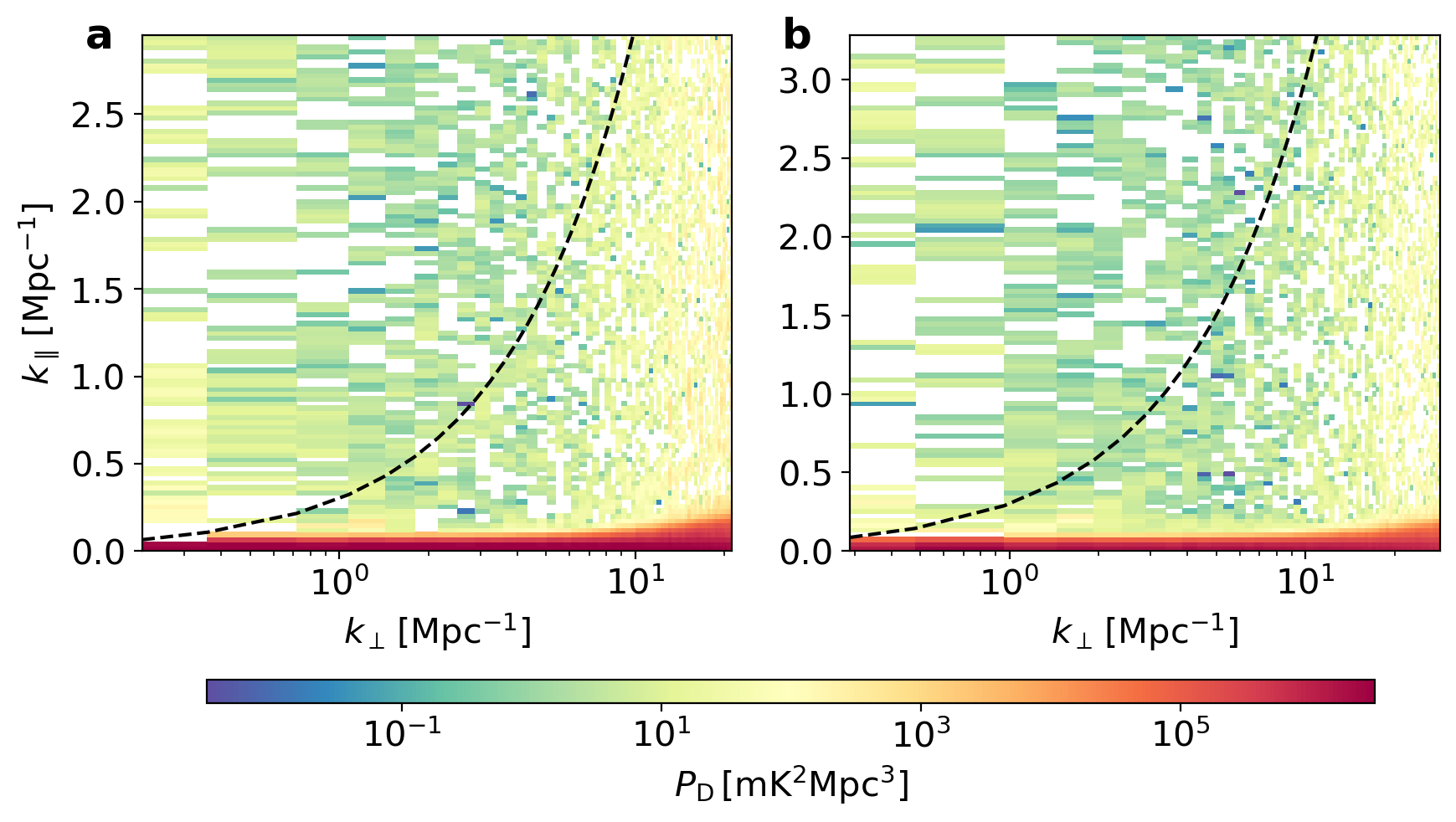
Figure 2: 2-d power spectrum from the analysis of $\mathbf{96}$-hrs MeerKAT interferometer data at $\mathbf{z=0.32}$ and $\mathbf{z=0.44}$. a, with Stokes I visibility data, cross-correlating the even and odd scan cubes for ${z=0.32}$. b, for $z=0.44$. Negative values are left blank. The $(\bm{k_{\perp}},k_{\parallel})$ modes above the black dashed line $(k_{\parallel}>0.3k_{\perp})$ are used to calculate the 1-d power spectrum.

In Figure 2, we show the 2-d power spectrum as a function of $(k_{\perp},k_{\parallel})$ at $z=0.32$ and $z=0.44$. The dashed line in Figure 2 defines the wedge, $k_{\parallel}=0.3k_{\perp}$, above which we do not expect any foreground contamination (e.g. Morales et al. 2012). In our case, the superb stability of MeerKAT and its primary beam size move the contaminants to a much smaller region. Nevertheless, we take a conservative approach and restrict our analysis to values above the dashed line. This foreground avoidance technique has the advantage of being robust to signal loss. Apart from the foreground-dominated modes at low $k_{\parallel}$, the rest of the cylindrical $k$-space is largely noise-dominated.

We further average the power spectrum into bins in $k$ to increase the statistical significance. For each redshift bin, we choose 7 logarithmic $k$-bins and average the 3-d powers into the 1-d power spectrum with inverse covariance weighting described in Equation 5 and Equation 6. The resulting 1-d HI power spectra are shown in Figure 3. For both redshifts, the 1-d power spectrum shows a clear detection, with the statistical significance being $8.0\sigma$ and $11.5\sigma$ respectively for $z=0.32$ and $z=0.44$. The measured power spectrum drops as $k$ increases which is expected. The amplitude of the signal at small scales is $\sim 0.1\,{\rm mK^{2}Mpc^{3}}$, consistent with the combination of the expected shot noise level of $\sim 1\,{\rm mK^{2}Mpc^{3}}$ (e.g. Chen et al. (2021)) and heavy attenuation due to the Finger-of-God (FoG) effects at high $k_{\parallel}$. For both redshifts, second $k$-bins of the power spectrum is lower than expected. This is due to the systematics at short baselines $u\approx 0$ as we show in Appendix A. While the systematics are largely removed, some weak effects may not be picked up by the $5-\sigma$ flagging. It does not impact the robustness of our detection, because the expected amplitude of the power spectrum is still well within the $3-\sigma$ region of our measurements. Furthermore, since we use the sampling variance for calculating the measurement errors, the impact of the systematics is incorporated and results in larger error bars. As a result of the low power spectrum amplitude at the second $k$-bin, when we perform the model fitting in section 4, the median fitting results are biased towards lower values for the first $k$-bin as seen in Figure 5 and Figure 6.

To validate our results, we perform a null test by cross-correlating the data of the two frequency sub-bands used in the detection. The individual sub-bands have no overlap and each of them is split into two time blocks of even and odd scans. When calculating the cross-power, only $k$-points that are above the $k_{\parallel}=0.3k_{\perp}$ wedge and not flagged by the $5-\sigma$ criterion are used. Therefore, the cross-power should give results consistent with zero. As shown in Figure 4, we detect no significant correlation in these tests which shows that no obvious frequency correlated signals remain in the Fourier window used in the analysis. The null test suggests that the observation window we choose does not have sizeable foreground leakage, and residual systematics have been largely mitigated.

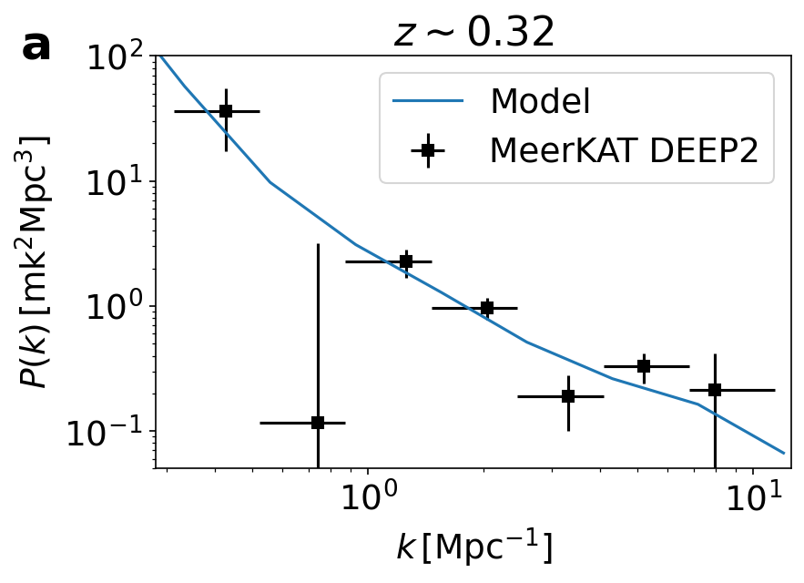
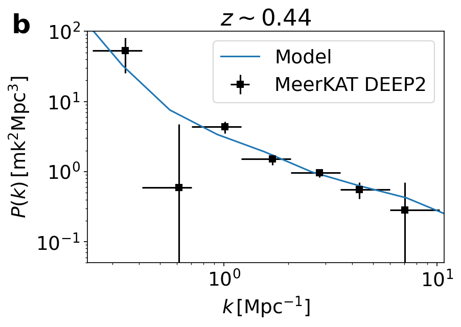
Figure 3: 1-d power spectrum from the analysis of the MeerKAT DEEP2 data. a, at $z=0.32$ and b, $z=0.44$. The measurement is denoted as “MeerKAT DEEP2” and the expected level of signal denoted as “Model” is calculated following the best fit results of the “No Prior” case in section 4.

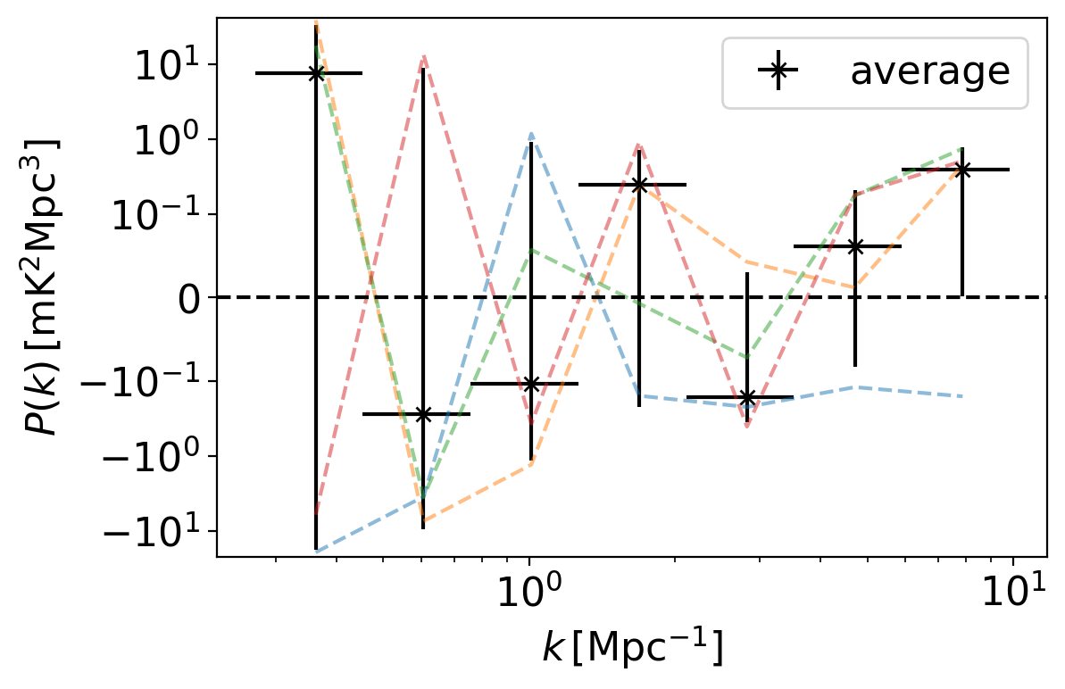
Figure 4: Null test– cross power spectrum between the two redshift bins. As each redshift bin has been divided into two time bins of even and odd scans, we have four possible cross-correlations between the two redshift bins, shown as the dashed lines. The black data points shows the average of the four cases and we observe no significant correlation. The value of the $k$ bins and normalization of the power spectrum are calculated at $1032$ MHz which is approximately midway to the central frequencies of the two redshift bins. The error bars are calculated by taking the sampling variance of the four cases.

$z=0.32$				$z=0.44$
$k$[Mpc-1]	$P(k)$[mK2Mpc3]	$\sigma_{P}$[mK2Mpc3]	$P(k)/\sigma_{P}$	$k$[Mpc-1]	$P(k)$[mK2Mpc3]	$\sigma_{P}$[mK2Mpc3]	$P(k)/\sigma_{P}$
0.43	36.48	19.03	1.92	0.34	53.43	27.80	1.92
0.74	0.12	3.04	0.04	0.61	0.60	4.13	0.14
1.25	2.26	0.57	3.98	1.01	4.34	0.85	5.12
2.04	0.96	0.19	4.96	1.68	1.51	0.27	5.62
3.30	0.19	0.09	2.12	2.81	0.96	0.13	7.54
5.19	0.33	0.09	3.80	4.31	0.56	0.15	3.80
7.96	0.21	0.20	1.07	7.04	0.28	0.41	0.69

Table 1: Table summarizing the HI power spectrum constraints at $z=0.32$ and $z=0.44$. From left to right, the columns show the centre of each $k$-bin, the value of the measured HI power spectrum in the units of mK²Mpc³, the measurement uncertainties in the units of mK²Mpc³, and the significance of the detection in each $k$-bin.

To further quantify the amplitude of the HI fluctuations measured, we use the 3-d power from our data to compute the variance of the fluctuation at a given scale R

$$\sigma_{\rm HI}^{2}=\frac{3}{4\pi R^{3}}\,\frac{\int_{k_{\rm window}}\frac{{\rm d}^{3}k}{(2\pi)^{3}}W^{2}(kR)P_{\rm D}(\bm{k})w(\bm{k})}{\int_{k_{\rm window}}\frac{{\rm d}^{3}k}{(2\pi)^{3}}W^{2}(kR)w(\bm{k})},$$ (7)

where the integration sums over all the $k$-pixels in the delay-transformed visibility data cube and $w(\bm{k})$ is the inverse covariance weight discussed before. $W(kR)=3j_{1}(kR)/(kR)$ is the Fourier transform of the spherical top-hat function with $j_{1}$ being the spherical Bessel function of the first kind.

As shown in Table 1, our measurements are most sensitive to scales around 1.0 Mpc. We use the bootstrapping method to estimate $\sigma_{\rm HI}$ at $R=1.0$ Mpc, by running 8000 realizations with each realization selecting $10^{4}$ k-pixels that are not flagged. In each realization, a value of $\sigma_{\rm HI}$ is calculated according to the $k-$pixels selected. This allows us to constrain the rms of HI density to be $\sigma_{\rm HI}=(0.44\pm 0.04)\,{\rm mK}$ at $z\sim 0.32$ and $\sigma_{\rm HI}=(0.63\pm 0.03)\,{\rm mK}$ at $z\sim 0.44$, at the scale of 1.0 Mpc. The results for $\sigma_{\rm HI}$ coherently sum over all $k$-points used, and thus can be used as an indicator for the overall statistical significance of the measurements. Our results have high statistical significance of our detections at both redshifts, demonstrating the capability of MeerKAT observations for interferometric HI intensity mapping.

4 Model fitting

In this section, we use the obtained measurement of the HI power spectrum to constrain the astrophysics of the HI galaxies and the HI mass function (HIMF) following Chen et al. (2021). The power spectrum is modelled as a combination of a 2-halo and 1-halo term as well as a scale-independent shot noise term. We further include redshift space distortions, e.g. the Kaiser term (Kaiser, 1987) which increases the amplitude of the power spectrum on large scales and the “fingers-of-god” term (Jackson, 1972) which smooths out fluctuations on small scales. The theoretical power spectrum is averaged in the same way as the observed one in order to produce the 1-d power spectrum.

We model the HI power spectrum as a combination of a 2-halo, 1-halo, and shot noise term (Cooray & Sheth, 2002; Wyithe & Brown, 2010; Chen et al., 2021):

$$P_{\rm D}(k_{\perp},k_{\parallel})=P_{\rm 2h}(k_{\perp},k_{\parallel})+P_{\rm 1h}(k_{\perp},k_{\parallel})+P_{\rm SN}(k_{\parallel}).$$ (8)

The 2-halo term can be modelled as

$$\begin{split}P_{\rm 2h}(k,k_{\parallel})=&C_{\rm HI}^{2}\bigg{[}\int{\rm d}n\,n(m)b(m)\langle M_{\rm HI}(m)\rangle u_{\rm HI}(k|m)\bigg{]}^{2}(1+\frac{fk_{\parallel}^{2}}{b_{\rm HI}^{0}k^{2}})^{2}\frac{P_{m}(k)}{{1+(k_{\parallel}\sigma_{p})^{2}}/2},\end{split}$$ (9)

where $m$ integrates over the halo mass range, $C_{\rm HI}$ is the conversion factor from HI mass density to temperature, $n(m)$ is the halo mass function (Tinker et al., 2008), $b(m)$ is the linear halo bias (Tinker et al., 2010), $\langle M_{\rm HI}(m)\rangle$ is the HI-halo mass relation, $u_{\rm HI}(k|m)$ is the normalised Fourier-transformed density profile, $k=\sqrt{k_{\perp}^{2}+k^{2}_{\parallel}}$ and $b_{\rm HI}^{0}$ is the linear HI bias. We include redshift space distortions in our analysis, taking into account both the Kaiser effect (Kaiser, 1987) as well as the FoG effect (Jackson, 1972) which affects the small line of sight scales (large $k_{\parallel}$) we are observing. For these terms, $f$ is the growth rate and $\sigma_{p}=\sigma_{v}(1+z)/(Hf)$ where $\sigma_{v}$ is the velocity dispersion and $H$ is the Hubble parameter. Here, we simplify the modelling of the FoG effects by assuming an averaged velocity dispersion $\sigma_{v}$, which can be related to the velocity width of the emission line profile of the stacked HI galaxies. $P_{\rm m}(k)$ is the matter power spectrum calculated using halofit (Takahashi et al., 2012).

The linear HI bias is calculated as

$$b_{\rm HI}^{0}=\frac{\int{\rm d}n\,n(m)b(m)\langle M_{\rm HI}(m)\rangle}{\int{\rm d}n\,n(m)\langle M_{\rm HI}(m)\rangle},$$ (10)

while the 1-halo term can be modelled as

$$P_{\rm 1h}(k,k_{\parallel})=C_{\rm HI}^{2}\int{d}n\,n(m)\langle M_{\rm HI}(m)\rangle^{2}u_{\rm HI}(k|m)\frac{1}{{1+(k_{\parallel}\sigma_{p})^{2}}/2}.$$ (11)

The shot noise term $P_{\rm SN}(k_{\parallel})$ can be written as

$$P_{\rm SN}(k_{\parallel})=\frac{P_{\rm SN}^{0}}{1+(k_{\parallel}\sigma_{p})^{2}/2}.$$ (12)

Note that, the shot noise in the HI power spectrum is also attenuated by the FoG effect. This is due to the fact that the HI sources are not treated as point sources on the sky but as intensity maps. The emission line width, corresponding to the velocity dispersion of the sources, breaks the point-source assumption along the line of sight, smearing the overall power spectrum along the $k_{\parallel}$ direction.

We further parameterize:

$$\langle M_{\rm HI}(m)\rangle=A_{\rm HI}\big{(}\frac{m}{M_{0}}\big{)}^{\beta},\,\rho_{\rm HI}(r|m)=\rho_{0}\big{(}\frac{r}{r_{0}}\big{)}^{\gamma}{\rm exp}[-ar/r_{0}],$$ (13)

where $M_{0}=10^{10}M_{\odot}{\rm h}^{-1}$, $r$ is the distance relative to the halo centre, and $r_{0}$ is the characteristic scale of the dark matter halo, calculated using the concentration-mass relation (Macciò et al., 2007). The parameter $a$ is fixed by imposing that at $m=10^{12}M_{\odot}{\rm h}^{-1}$ the cut-off scale is $r_{0}/a=1{\rm Mpc\,h^{-1}}$ (Spinelli et al., 2020). We further fix the power law index for the velocity dispersion as in (Villaescusa-Navarro et al., 2018), which leaves us with a 5-parameter model:

$$\theta=\{A_{\rm HI},\beta,\gamma,\sigma_{v},P_{\rm SN}^{0}\}.$$ (14)

After choosing the halo model parameters, we compute the analytical power spectrum using halomod (Murray et al., 2021) and average across the k-range probed as shown in Figure 2. We construct a Gaussian likelihood from the results reported and use emcee (Foreman-Mackey et al., 2013) to fit for the model parameters with 50 random walkers and 8000 steps to ensure convergence. We discard the first 2000 steps. Flat priors are imposed so that all parameters are positive. For $\gamma$, we impose $1<\gamma<3$ since values outside this range lead to divergence. From the stacking of selected HI galaxies using MeerKAT observations at similar redshifts (Sinigaglia et al., 2022), we impose a flat prior on the velocity dispersion $0<\sigma_{v}<500\,{\rm km\,s^{-1}}$. The HOD parameters $A_{\rm HI}$ and $\beta$ are specific to the parameterization, and their physical meanings can be hard to interpret. Therefore, in each sample in the posterior, we calculate $\Omega_{\rm HI}$ and the HI bias $b_{\rm HI}$ at 1.0 Mpc^-1 and present the results with these two parameters instead of $A_{\rm HI}$ and $\beta$.

As we show later, the parameter fitting does not converge for all parameters due to parameter degeneracy and lack of information on the $k_{\parallel}$ dependence of the power spectrum. We therefore consider another case where we impose a prior on $\Omega_{\rm HI}$ with $\Omega_{\rm HI}=(0.50\pm 0.18)\times 10^{-3}$ at $z\sim 0.32$ from stacking (Rhee et al., 2018) and $\Omega_{\rm HI}=(0.77\pm 0.26)\times 10^{-3}$ at $z\sim 0.44$ from Damped Lyman Alpha (DLA) systems (Rao et al., 2017).

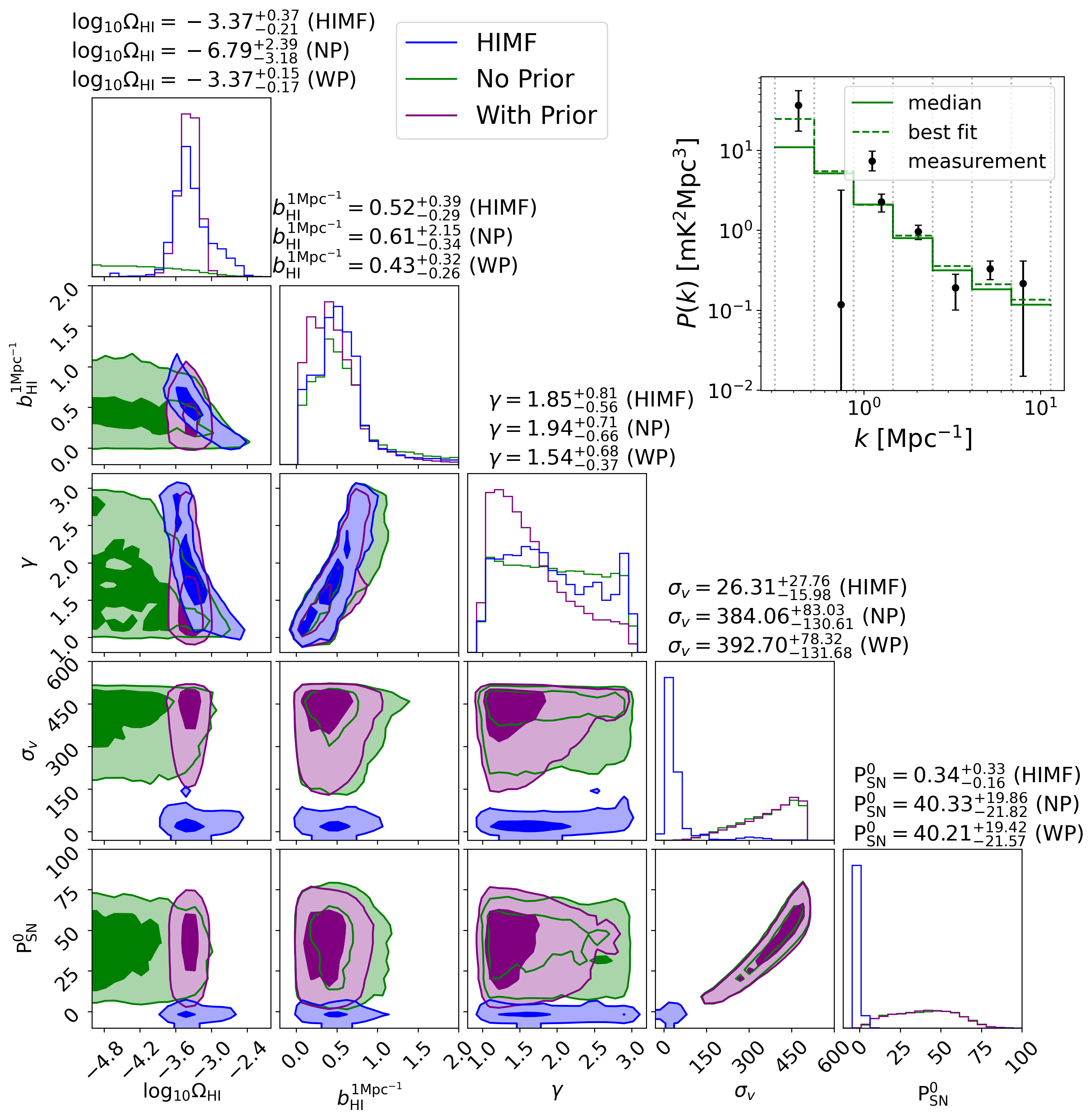
Figure 5: Model fitting results for $z\sim 0.32$. The 2-d contour plots show posterior distribution of model parameters for power spectrum fitting. The darker region shows the $1\sigma$ confidence interval of the posterior and the lighter region shows the $2\sigma$ confidence interval. $\sigma_{v}$ is shown in the unit of km/s. $P_{\rm SN}$ is shown in the unit of $\rm mK^{2}Mpc^{3}$. The upper lines of the titles of the 1-d histograms show the median and the $1\sigma$ confidence level for each parameter for the model fitting with the shot noise modelled by the HIMF (“HIMF”). The middle lines of the titles of the 1-d histograms show the results without the $\Omega_{\rm HI}$ prior (“NP”). The lower lines show the results with the $\Omega_{\rm HI}$ prior (“WP”). The 2-d posterior distribution is smoothed with a Gaussian kernel of 0.5 grid width for better visualization. In the upper right zoom-in panel, the fitting result of the power spectrum measurement with no prior is shown. The vertical dash line shows the lower and upper limit for each k-bin.

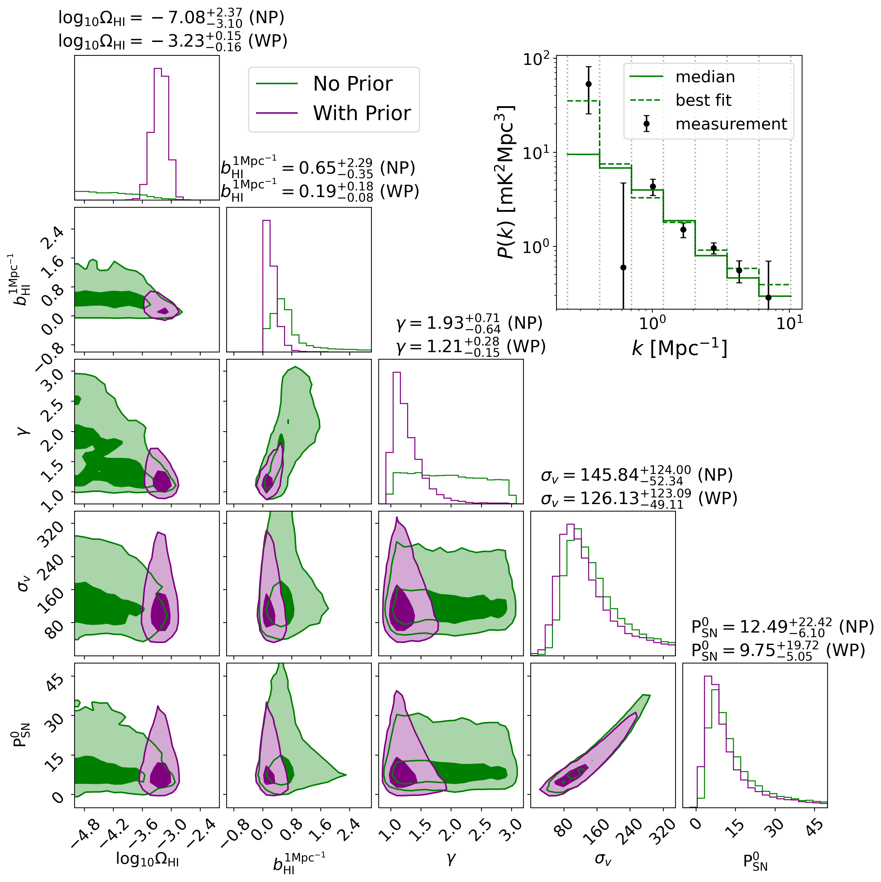
Figure 6: Model fitting results for $z\sim 0.44$. The 2-d contour plots show posterior distribution of model parameters for power spectrum fitting. The darker region shows the $1\sigma$ confidence interval of the posterior and the lighter region shows the $2\sigma$ confidence interval. $\sigma_{v}$ is shown in the unit of km/s. $P_{\rm SN}$ is shown in the unit of $\rm mK^{2}Mpc^{3}$. The upper lines of the titles of the 1-d histograms show the median and the $1\sigma$ confidence level for each parameter for the model fitting without the $\Omega_{\rm HI}$ prior (“NP”). The lower lines show the results with the $\Omega_{\rm HI}$ prior (“WP”). The 2-d posterior distribution is smoothed with a Gaussian kernel of 0.5 grid width for better visualization. In the upper right zoom-in panel, the fitting result of the power spectrum measurement with no prior is shown. The vertical dash line shows the lower and upper limit for each k-bin.

The fitting results are shown in Figure 5 for $z\sim 0.32$ and Figure 6 for $z\sim 0.44$. The green regions show the posterior distribution for the model parameters without the $\Omega_{\rm HI}$ priors while the purple region shows the distribution with the prior. The blue regions show the results with the HIMF modelling which we discuss later. From the posterior, one can see that the small number of $k$-bins and the relatively low signal-to-noise ratio lead to divergence in the MCMC fitting, with most of the parameters unconstrained. The constraints on $\Omega_{\rm HI}$ are noticeably worst if no prior is imposed. This is expected, since the small inner-halo scales do not contain enough information to constrain the overall amplitude which is on the large scales. The density profile parameter $\gamma$ is also poorly constrained, because the small scale power spectrum is dominated by the effects of the shot noise and the velocity dispersion.

Comparing the results at $z\sim 0.32$ and $z\sim 0.44$, one can see that both redshift bins show tangible evidence that the velocity dispersion $\sigma_{v}$ and the HI shot noise can be jointly constrained. For $z\sim 0.32$, the posterior is reaching the flat prior $\sigma_{v}<500\,{\rm km/s}$ we impose. We verify that relaxing this prior simply leads to the posterior streching to higher, more unphysical values of $\sigma_{v}$. The large tail of the $\sigma_{v}$ distribution also drives the shot noise $P_{\rm SN}^{0}$ to be larger, since these two parameters are degenerate. The $z\sim 0.44$ redshift bin has higher signal-to-noise ratio and the results give a reasonable constraint on the velocity dispersion $\sigma_{v}=145.84^{+124.00}_{-52.34}\,{\rm km/s}$, although the problem of the degeneracy between $\sigma_{v}$ and $P_{\rm SN}^{0}$ persists. This is again expected for our preliminary result. The cylindrical power spectrum for the DEEP2 data is dominated by thermal noise, and therefore we need to average the $k$-pixels down to 1-d power spectrum in order to constrain our model. Binning the cylindrical power spectrum into 1-d power spectrum means that we lose the information along the $k_{\parallel}$ direction, which entails the effects of the $\sigma_{v}$ parameter. In the future with more data resulting in higher signal-to-noise ratio, binning the $k$-points into $k_{\perp}-k_{\parallel}$ grids will help preserve the $k_{\parallel}$ dependence of the FoG effect, breaking the degeneracy between $\sigma_{v}$ and the rest of the parameter set. The degeneracy can also be resolved by using the HIMF to model the shot noise instead of treating it as a free parameter, which we discuss later in this section.

Comparing the results with and without the $\Omega_{\rm HI}$ prior, we find that the fitting converges on the $\Omega_{\rm HI}$ parameter as expected, but shows no visible improvement for shot noise and velocity dispersion. For $z\sim 0.44$ with better signal-to-noise ratio, we start to be able to constrain the density profile parameter $\gamma$, which leads to better constraints on the HI bias at small scales. The results suggest that at 1-D power spectrum level, the signal at the scales of the measurement is dominated by the 1-halo term and the shot noise, which are less correlated with the overall HI amplitude comparing to the large scales dominated by the 2-halo term.

Our results show that using MeerKAT interferometric observations, we can constrain the velocity dispersion and the HI shot noise even with preliminary measurements with relatively low signal-to-noise ratio. In the future with more data from the MeerKAT observations, intensity mapping measurements can be used to constrain the halo model of HI, providing a detailed picture of the galaxy evolution from $z\sim 0.0$ to $z\sim 1.0$.

The measurements on the HI shot noise can also be used to constrain the HI mass function (Chen et al., 2021). The HIMF is parameterized with a Schechter function (Schechter, 1976):

$$\phi_{\rm HI}(M_{\rm HI})\equiv\frac{{\rm d}n_{\rm HI}}{{\rm dlog}M_{\rm HI}}={\rm ln}10\,\phi_{*}\big{(}\frac{M_{\rm HI}}{M_{*}}\big{)}^{\alpha+1}e^{-\frac{M_{\rm HI}}{M_{*}}}.$$ (15)

This can be related to the number density, $n_{\rm HI}$, HI mass density and shot noise as:

$$n_{\rm HI}=\int_{M_{\rm min}}{\rm dlog}M_{\rm HI}\,\phi_{\rm HI}(M_{\rm HI})$$ (16)

$$\Omega_{\rm HI}=\int{\rm dlog}M_{\rm HI}\,\phi_{\rm HI}(M_{\rm HI})M_{\rm HI}/\rho_{c}$$ (17)

$$P_{\rm SN}^{0}=(C_{\rm HI}\rho_{c}\Omega_{\rm HI})^{2}\frac{\int{\rm dlog}M_{\rm HI}\,\phi_{\rm HI}(M_{\rm HI})M_{\rm HI}^{2}}{\big{(}\int{\rm dlog}M_{\rm HI}\,\phi_{\rm HI}(M_{\rm HI})M_{\rm HI}\big{)}^{2}}$$ (18)

For intensity mapping experiments, we have independent measurements for $\Omega_{\rm HI}$ and $P_{\rm SN}^{0}$. For $n_{\rm HI}$ we need external information since the 1-halo and 2-halo terms are only sensitive to the HI density distribution inside halos and not the number of HI galaxies itself. The ideal approach is to use HI stacking of the same field that we are observing. Here, however, we are only interested in a proof-of-concept to illustrate its feasibility on future MeerKAT data. We use the reported number density (165 galaxies in a 57’ field) and average HI mass ($\langle M_{\rm HI}\rangle=(5.73\pm 1.47)\times 10^{9}M_{\odot}$ ) of the stacking sample in Rhee et al. (2018). For $\Omega_{\rm HI}$ and $P_{\rm SN}$, intensity mapping observations integrate over all the HI mass and therefore the integration limit is chosen to be $10^{7}$ to $10^{13}$ solar masses for convergence. The number density, on the other hand, depends on the lower mass limit of the stacking sample. In order to incorporate the ignorance of this minimum mass and use the stacking result as a prior in our model fitting, we use the following routine in the MCMC:

• In each step, a random set of halo model parameters as well as the HIMF parameters $\phi_{*}$ and $M_{*}$ is sampled.

• Based on the halo model parameter, the overall HI density $\Omega_{\rm HI}$ is calculated. Using Equation 17, we can calculate the value for the last HIMF parameter $\alpha$.

• The shot noise is calculated using Equation 18.

• Using the number density $n_{\rm HI}=2.987\times 10^{-3}\,{\rm Mpc^{-3}}$ corresponding to 165 galaxies in a 57’ field, from Equation 16 we can find the lower mass limit of the stacking sample.

• From the lower mass limit, we randomly sample 165 galaxies from the HIMF distribution. The average HI mass of the samples $\bar{M}_{\rm HI}$ is compared against the stacking result $\langle M_{\rm HI}\rangle=(5.73\pm 1.47)\times 10^{9}M_{\odot}$. A Gaussian prior can be calculated as part of the likelihood ${\rm log[p]}=-0.5\times(\bar{M}_{\rm HI}/10^{9}M_{\odot}-5.73)^{2}/1.47^{2}$.

Incorporating the HIMF into our model fitting, the shot noise $P_{\rm SN}^{0}$ is no longer a free parameter. Instead, it is derived from the HIMF and the halo model parameters, making the fitting results on the model parameters different from the previous cases shown. The updated results using the measurements at $z\sim 0.32$ are shown as the blue regions in Figure 5. Comparing the results with previous fittings where shot noise is treated as a free parameter, we find that the shot noise is no longer biased towards larger values. This is due to the fact that, in order to get to the large values for the shot noise, the HIMF needs to be skewed towards the higher mass end. On the other hand, the parameter space where the HIMF is skewed towards the higher mass end is disfavoured by the MCMC fitting, because it would result in a much higher average HI mass when we sample the 165 HI galaxies. Comparing the fitting with the HIMF with a naive $\Omega_{\rm HI}$ prior, we can see that, apart from the shot noise no longer being biased, the posterior also shows anti-correlation between $\Omega_{\rm HI}$ and $b_{\rm HI}$. The anti-correlation suggests that the information from stacking provides extra constraints for the large scale, leading to the degeneracy between the HI density and the bias as they equally contribute to the power spectrum amplitude. In conclusion, using the HIMF to model the shot noise helps excluding part of the parameter space that is not physical, resulting in better constraints for the parameters.

We note that, however, the fitted values for $\sigma_{v}$ and $P_{\rm SN}^{0}$ are much lower than the results without the HIMF parameters. It is possible that the stacking sample we are using is not complete, making the HIMF lower than the underlying truth. As the HIMF is lower, the shot noise is also lower and to compensate the drop in the power spectrum amplitude, the velocity dispersion becomes smaller as well. This issue can be mitigated by using the MeerKAT DEEP2 data itself to perform HI galaxy stacking, which we leave for future work. Here, we are only interested in demonstrating the effects of using the HIMF in the model fitting to improve the constraints on HI, which is evident in the posterior. Our findings strongly advocates for combined constraints on HI galaxies from the same MeerKAT observations using both stacking and intensity mapping techniques. The intensity mapping measurements in turn help constrain the HIMF parameters, without the need to resolve individual galaxies or split galaxy samples, significantly extending the redshift range where the HIMF can be probed comparing to the conventional HI galaxy stacking technique.

In Figure 7, we show the posterior distribution of the HIMF parameters as well as the fitted HIMF at $z\sim 0.32$. The HI power spectrum is more sensitive to the “knee mass” $M_{*}$ and the slope parameter $\alpha$ while being less sensitive to the overall abundance $\phi_{*}$, since the HI shot noise is weighted by the HI mass squared and therefore sensitive to the relative abundance of the HI-heavy galaxies. Comparing our results to the HIMF measured at the local Universe (Jones et al., 2018), we find a lower “knee mass”, suggesting that galaxies obtain more HI from $z\sim 0.32$ to $z\sim 0.0$. Our findings are also consistent with measurements of the HIMF at similar redshift (Bera et al., 2022). It is also consistent with the MIGHTEE-HI measurements of the scaling relations (Sinigaglia et al., 2022; Pan et al., 2022). In the future, combining measurements of intensity mapping and HI galaxy surveys using MIGHTEE survey data (Maddox et al., 2021), we will be able to probe the HIMF from $z\sim 0.0$ to $z\sim 0.5$, opening up a new window into studying the evolution of the star-forming properties of galaxies.

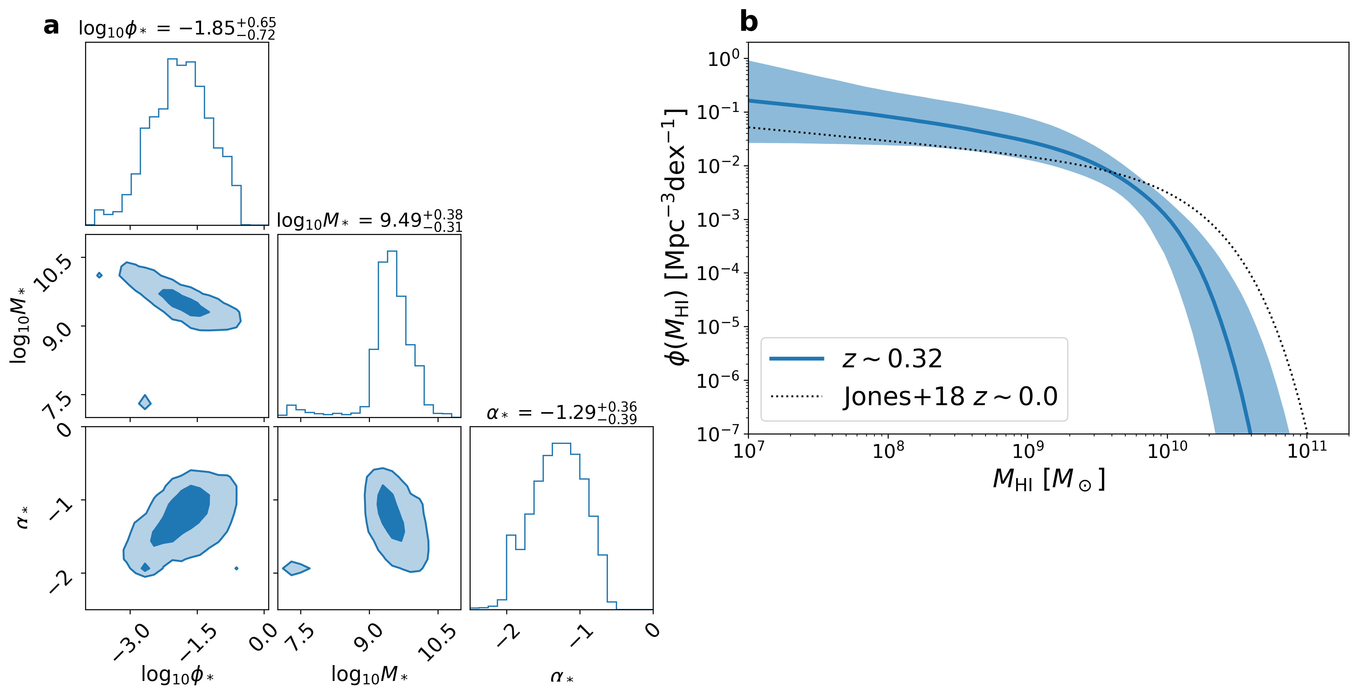
Figure 7: Measurement of HIMF parameters for power spectrum fitting at $z\sim 0.32$. a, the darker region shows the $1\sigma$ confidence interval of the posterior and the lighter region shows the $2\sigma$ confidence interval. $\phi$ is shown in the unit of $\rm Mpc^{-3}dex^{-1}$. $M_{*}$ is shown in the unit of solar mass. The titles of the 1-d histograms show the median and the $1\sigma$ confidence level for each parameter. The 2-D posterior distribution is smoothed with a Gaussian kernel of 0.5 grid width for better visualization. b, the $1\sigma$ region of the fitted HIMF is shown in blue with the solid line being the mean. The result from HI galaxy survey in the local Universe (Jones et al., 2018) is shown in dotted line for comparison.

5 Conclusion

In this letter, we use the MeerKAT observations of the DEEP2 field to make the first-ever detection of the HI autopower spectrum at $z\sim 0.32$ and $z\sim 0.44$. The deep observations allow accurate calibration of the data with errors $\sim 10^{-5}$. Splitting the frequency range into two sub-bands, each with 220 frequency channels centred around $z\sim 0.32$ and $z\sim 0.44$, we cross-correlate the visibility data from different timeblocks to minimise time-dependent systematics and remove noise bias. The resulting power spectrum measurements in the $k_{\parallel}>0.3k_{\perp}$ region are binned into 1-d $k$-bins. The HI power spectrum at both redshifts is measured with high statistical significance. Cross-correlating the timeblocks between the two frequency sub-bands as a null test, we find the cross-power spectrum fluctuates around zero with no indication of excess power, suggesting that our measurements are free of foreground leakage. Residual systematic effects are mitigated by $5$-$\sigma$ flagging in $k$-space using thermal noise simulations derived from the Stokes V data.

The resulting HI power spectrum is then used to perform parameter inference. Using halo model formalism to calculate the HI power spectrum and including the effects of redshift space distortion, we find that the scales probed by our measurements are dominated by the combination of the HI shot noise and the velocity dispersion. Due to the fact that the power spectrum is measured in 1-d $k$-bins, losing the information of the $k_{\parallel}$ dependence, the parameters are degenerate with each other, leading to a divergence in the fitting. Imposing a $\Omega_{\rm HI}$ prior based on existing constraints, we find that preliminary constraints on the HI shot noise, the velocity dispersion, and the HI density profile can be made. We also demonstrate that incorporating the HI mass function into the modelling can help mitigate divergence for the shot noise and the velocity parameters, yielding better constraints. The HI mass function itself can in turn be constrained.

Our results show that it is possible to isolate the HI signal from the strong foregrounds using the avoidance technique and obtain a high signal to noise detection, opening the window to observational cosmology on quasi-linear scales. These measurements can be used to extract astrophysical information on the HI galaxies, informing us on the accuracy of current hydrodynamic HI simulations (Davé et al., 2019). MeerKAT surveys such as MIGHTEE (Taylor & Jarvis, 2017) and Laduma (Blyth et al., 2016) are currently undertaking deep observations on several fields which will allow to measure the small scale HI power spectrum to extreme precision and provide exquisite constraints on the HI mass function, the halo model and the nature of redshift space distortions on these scales.

Data availability

The uncalibrated visibility data used in this work are publicly available under the Proposal ID: SCI-20180426-TM-01 in SARAO archive (https://archive.sarao.ac.za).

Code availability

The initial processing and calibration of the MeerKAT data was carried out using the processMeerKAT pipeline developed at the IDIA and available at https://idia-pipelines.github.io/docs/processMeerKAT. The self calibrations were performed with standard CASA tasks: tclean, gaincal and applycal (https://casa.nrao.edu/casa_obtaining.shtml). Further codes are available on a reasonable request to the authors.

Appendix A Removing Residual Systematics

We present further details of using the thermal noise simulation to flag systematics in the data. For the gridded visibility data of the two frequency sub-bands, there exists a common feature of systematic effects that can been seen in the cylindrical power spectrum. For reference, in Figure 8, we show the same cross-power spectra of the two frequency bins as in Figure 2, but without the mitigation of systematics. Around the $k_{\parallel}=0.3k_{\perp}$ line, we can see a stripe of excess power. This stripe is present at both frequency bins and is unlikely to be of astrophysical origins. Since the systematic effects exist inside the observation window where foregrounds are avoided, we need to remove this excess power to enable the detection. In this work, we use thermal noise simulations to calculate the variance of the power spectrum in each 3-d $k$-pixel and mask values that are outside the 5$\sigma$ range as mentioned before.

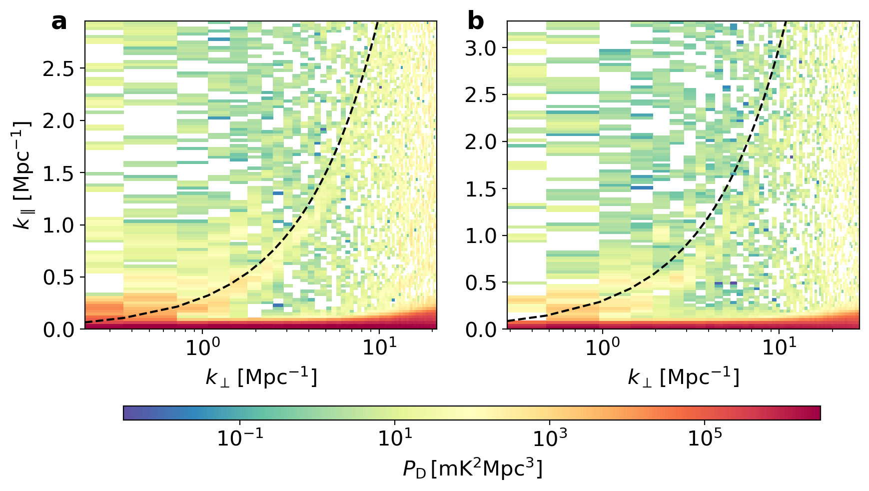
Figure 8: 2-d power spectrum from the analysis of $\mathbf{96}$-hrs MeerKAT interferometer data at $\mathbf{z=0.32}$ and $\mathbf{z=0.44}$ without the mitigation of the systematics. a, with Stokes I visibility data, cross-correlating the even and odd scan cubes for ${z=0.32}$. b, for $z=0.44$. Negative values are left blank. The $(\bm{k_{\perp}},k_{\parallel})$ modes above the black dashed line $(k_{\parallel}>0.3k_{\perp})$ are used to calculate the 1-d power spectrum.

We first use the Stokes V data to estimate the amplitude of the thermal noise. The Stokes V mode is a good estimator of the thermal noise as the extragalactic foreground sources have minimal circular polarization. For MeerKAT observations, the Stokes V data is consistent with the thermal noise at long baselines (Paul et al., 2021). We use the same gridding routine as in section 2 to grid the Stokes V data without filling the flagged channels with the nearest neighbour, and use the gridded visibility to calculate the Stokes V power spectrum. Based on the number of baselines in each $u$-$v$ grid, we can calculate the thermal noise amplitude $\sigma_{N}$

$$\sigma_{N}={\rm std}(V_{i}\sqrt{N_{i}}),$$ (A1)

where $N_{i}$ is the (non-zero) number of baselines within each $u$-$v$ grid and $V_{i}$ is the averaged Stokes V visibility of each $u$-$v$ grid. The natural sensitivity $A_{e}/T_{\rm sys}$ is calculated using Equation 4. We find $A_{e}/T_{\rm sys}=6.65\,{\rm m^{2}/K}$ for $z=0.32$ and $6.48\,{\rm m^{2}/K}$ for $z=0.44$, consistent with the anticipated performance of the MeerKAT telescope and the fact that observations at lower frequencies should have slightly higher thermal noise. We can also use it to estimate that for the narrow 46MHz sub-bands, the natural sensitivity has a $\sim 1\%$ evolution which is negligible, since we cross-correlate different timeblocks to remove the thermal noise bias.

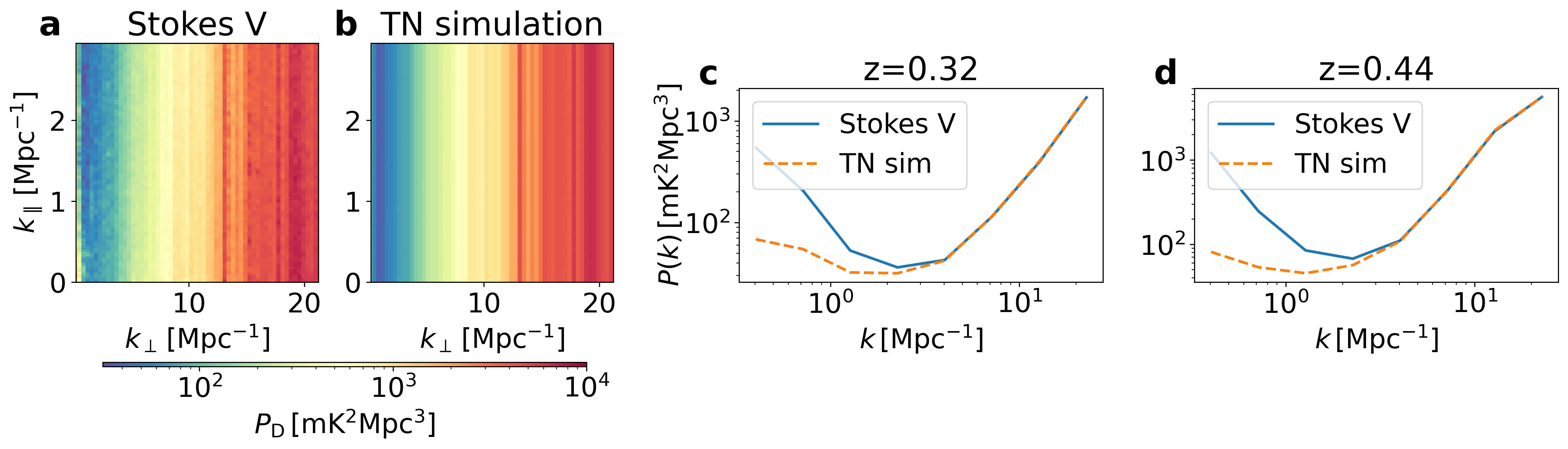
Figure 9: a, The cylindrical power spectrum of the Stokes V mode calculated from the $z=0.44$ data. The Stokes V mode is a good estimator of the thermal noise as the extragalactic foreground sources have minimal circular polarization. b, Simulated thermal noise power spectrum averaged across 10000 realizations for $z=0.44$. c, The 1-D power spectrum of the Stokes V mode compared against the thermal noise simulation for $z=0.32$. d, The 1-D power spectrum of the Stokes V mode compared against the thermal noise simulation for $z=0.44$.

For illustration, in Figure 9 we present the cylindrical power spectrum from the thermal noise simulation, compared against the Stokes V data at $z=0.44$. The Stokes V power spectrum agrees well with our thermal noise simulation, especially at long baselines (high $k_{\perp}$). At shorter baselines, the increasing level of systematics and polarization signal breaks the similarity. In the cylindrical $k$-space, the power spectrum measurements for Stokes V have relatively large variance, and therefore the Stokes V power spectrum shown in Figure 9 looks “blurry”. To demonstrate that the amplitude of the thermal noise agrees tightly with the data, in Figure 9 we also show the 1-D power spectrum for the Stokes V data and the thermal noise simulation for both redshift bins. As one can see, for large $k$ the thermal noise simulation is in excellent agreement with the Stokes V data for both sub-bands.

We then simulate 10000 realizations of thermal noise for the Stokes I data, and use them to flag the excess power visible in Figure 8 as discussed in section 2. Comparing the results in Figure 8 and Figure 2, we can see that indeed the systematic effects have been removed. Within the $k_{\parallel}>0.3k_{\perp}$ window, we find $\sim 1\%$ of the $k$-pixels are flagged, the majority of which is within the stripe structure.

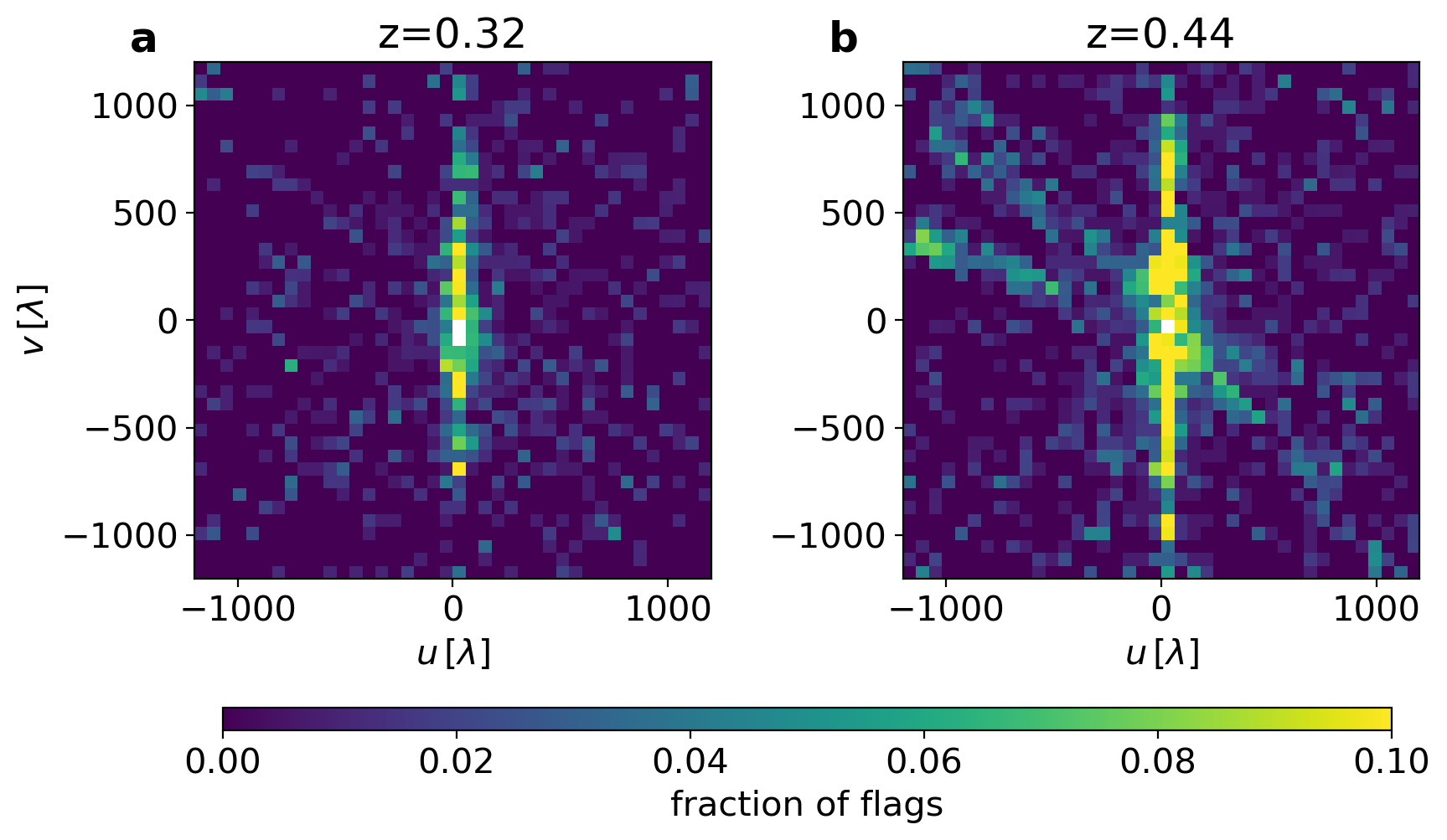
Figure 10: The fraction of flagged $\bm{k}$-pixels along the delay axis for a, $z=0.32$. b, $z=0.44$. Values above 10% are set to be 10% for better presentation.

To trace the origin of the systematics, we average across the delay axis within the observation window and show the fraction of flagged $k$-pixels for each $u$-$v$ grid in Figure 10. For both frequency sub-bands, the flagging is mostly visible near the $u=0$ line. This corresponds to a known issue for MeerKAT observations, whose origin is still under investigation.

References

- Anderson et al. (2018) Anderson, C. J., Luciw, N. J., Li, Y. C., et al. 2018, MNRAS, 476, 3382, doi: 10.1093/mnras/sty346
- Asad et al. (2021) Asad, K. M. B., Girard, J. N., de Villiers, M., et al. 2021, MNRAS, 502, 2970, doi: 10.1093/mnras/stab104
- Barry et al. (2016) Barry, N., Hazelton, B., Sullivan, I., Morales, M. F., & Pober, J. C. 2016, MNRAS, 461, 3135, doi: 10.1093/mnras/stw1380
- Battye et al. (2004) Battye, R. A., Davies, R. D., & Weller, J. 2004, MNRAS, 355, 1339, doi: 10.1111/j.1365-2966.2004.08416.x
- Bera et al. (2022) Bera, A., Kanekar, N., Chengalur, J. N., & Bagla, J. S. 2022, ApJ, 940, L10, doi: 10.3847/2041-8213/ac9d32
- Bharadwaj & Sethi (2001) Bharadwaj, S., & Sethi, S. K. 2001, Journal of Astrophysics and Astronomy, 22, 293, doi: 10.1007/BF02702273
- Blyth et al. (2016) Blyth, S., Baker, A. J., Holwerda, B., et al. 2016, in MeerKAT Science: On the Pathway to the SKA, 4, doi: 10.22323/1.277.0004
- Bull et al. (2015) Bull, P., Ferreira, P. G., Patel, P., & Santos, M. G. 2015, The Astrophysical Journal, 803, 21, doi: 10.1088/0004-637X/803/1/21
- Chang et al. (2010) Chang, T.-C., Pen, U.-L., Bandura, K., & Peterson, J. B. 2010, Nature, 466, 463, doi: 10.1038/nature09187
- Chen et al. (2023) Chen, Z., Wolz, L., & Battye, R. 2023, MNRAS, 518, 2971, doi: 10.1093/mnras/stac3288
- Chen et al. (2021) Chen, Z., Wolz, L., Spinelli, M., & Murray, S. G. 2021, MNRAS, 502, 5259, doi: 10.1093/mnras/stab386
- CHIME Collaboration et al. (2022) CHIME Collaboration, Amiri, M., Bandura, K., et al. 2022, arXiv e-prints, arXiv:2202.01242. https://arxiv.org/abs/2202.01242
- Chowdhury et al. (2020) Chowdhury, A., Kanekar, N., Chengalur, J. N., Sethi, S., & Dwarakanath, K. S. 2020, Nature, 586, 369, doi: 10.1038/s41586-020-2794-7
- Collier et al. (2021) Collier, J. D., Frank, B., Sekhar, S., & Taylor, A. R. 2021, in 2021 XXXIVth General Assembly and Scientific Symposium of the International Union of Radio Science (URSI GASS), 1–4, doi: 10.23919/URSIGASS51995.2021.9560276
- Comrie et al. (2021) Comrie, A., Wang, K.-S., Hsu, S.-C., et al. 2021, CARTA: Cube Analysis and Rendering Tool for Astronomy, Astrophysics Source Code Library, record ascl:2103.031. http://ascl.net/2103.031
- Cooray & Sheth (2002) Cooray, A., & Sheth, R. 2002, Phys. Rep., 372, 1, doi: 10.1016/S0370-1573(02)00276-4
- Cunnington et al. (2019) Cunnington, S., Wolz, L., Pourtsidou, A., & Bacon, D. 2019, MNRAS, 488, 5452, doi: 10.1093/mnras/stz1916
- Cunnington et al. (2023) Cunnington, S., Li, Y., Santos, M. G., et al. 2023, MNRAS, 518, 6262, doi: 10.1093/mnras/stac3060
- Datta et al. (2010) Datta, A., Bowman, J. D., & Carilli, C. L. 2010, The Astrophysical Journal, 724, 526, doi: 10.1088/0004-637x/724/1/526
- Davé et al. (2019) Davé, R., Anglés-Alcázar, D., Narayanan, D., et al. 2019, MNRAS, 486, 2827, doi: 10.1093/mnras/stz937
- Foreman-Mackey (2016) Foreman-Mackey, D. 2016, The Journal of Open Source Software, 1, 24, doi: 10.21105/joss.00024
- Foreman-Mackey et al. (2013) Foreman-Mackey, D., Hogg, D. W., Lang, D., & Goodman, J. 2013, PASP, 125, 306, doi: 10.1086/670067
- Harris et al. (2020) Harris, C. R., Millman, K. J., van der Walt, S. J., et al. 2020, Nature, 585, 357, doi: 10.1038/s41586-020-2649-2
- Hunter (2007) Hunter, J. D. 2007, Computing in Science and Engineering, 9, 90, doi: 10.1109/MCSE.2007.55
- Jackson (1972) Jackson, J. C. 1972, MNRAS, 156, 1P, doi: 10.1093/mnras/156.1.1P
- Jones et al. (2018) Jones, M. G., Haynes, M. P., Giovanelli, R., & Moorman, C. 2018, MNRAS, 477, 2, doi: 10.1093/mnras/sty521
- Kaiser (1987) Kaiser, N. 1987, MNRAS, 227, 1, doi: 10.1093/mnras/227.1.1
- Liu et al. (2014) Liu, A., Parsons, A. R., & Trott, C. M. 2014, Phys. Rev. D, 90, 023018, doi: 10.1103/PhysRevD.90.023018
- Liu & Shaw (2020) Liu, A., & Shaw, J. R. 2020, PASP, 132, 062001, doi: 10.1088/1538-3873/ab5bfd
- Macciò et al. (2007) Macciò, A. V., Dutton, A. A., van den Bosch, F. C., et al. 2007, MNRAS, 378, 55, doi: 10.1111/j.1365-2966.2007.11720.x
- Maddox et al. (2021) Maddox, N., Frank, B. S., Ponomareva, A. A., et al. 2021, A&A, 646, A35, doi: 10.1051/0004-6361/202039655
- Masui et al. (2013) Masui, K. W., Switzer, E. R., Banavar, N., et al. 2013, ApJ, 763, L20, doi: 10.1088/2041-8205/763/1/L20
- Mauch et al. (2020) Mauch, T., Cotton, W. D., Condon, J. J., et al. 2020, The Astrophysical Journal, 888, 61, doi: 10.3847/1538-4357/ab5d2d
- McMullin et al. (2007) McMullin, J. P., Waters, B., Schiebel, D., Young, W., & Golap, K. 2007, Astronomical Society of the Pacific Conference Series, Vol. 376, CASA Architecture and Applications, ed. R. A. Shaw, F. Hill, & D. J. Bell, 127
- McQuinn et al. (2006) McQuinn, M., Zahn, O., Zaldarriaga, M., Hernquist, L., & Furlanetto, S. R. 2006, The Astrophysical Journal, 653, 815, doi: 10.1086/505167
- Morales et al. (2012) Morales, M. F., Hazelton, B., Sullivan, I., & Beardsley, A. 2012, The Astrophysical Journal, 752, 137, doi: 10.1088/0004-637x/752/2/137
- Morales & Hewitt (2004) Morales, M. F., & Hewitt, J. 2004, The Astrophysical Journal, 615, 7, doi: 10.1086/424437
- Morales & Wyithe (2010) Morales, M. F., & Wyithe, J. S. B. 2010, ARA&A, 48, 127, doi: 10.1146/annurev-astro-081309-130936
- Murray et al. (2021) Murray, S. G., Diemer, B., Chen, Z., et al. 2021, Astronomy and Computing, 36, 100487, doi: 10.1016/j.ascom.2021.100487
- Olivari et al. (2016) Olivari, L. C., Remazeilles, M., & Dickinson, C. 2016, MNRAS, 456, 2749, doi: 10.1093/mnras/stv2884
- Pan et al. (2022) Pan, H., Jarvis, M. J., Santos, M. G., et al. 2022, arXiv e-prints, arXiv:2210.04651. https://arxiv.org/abs/2210.04651
- Parsons et al. (2012) Parsons, A., Pober, J., McQuinn, M., Jacobs, D., & Aguirre, J. 2012, The Astrophysical Journal, 753, 81, doi: 10.1088/0004-637X/753/1/81
- Parsons et al. (2014) Parsons, A. R., Liu, A., Aguirre, J. E., et al. 2014, The Astrophysical Journal, 788, 106, doi: 10.1088/0004-637x/788/2/106
- Paul et al. (2021) Paul, S., Santos, M. G., Townsend, J., et al. 2021, Monthly Notices of the Royal Astronomical Society, 505, 2039, doi: 10.1093/mnras/stab1089
- Paul et al. (2016) Paul, S., Sethi, S. K., Morales, M. F., et al. 2016, The Astrophysical Journal, 833, 213, doi: 10.3847/1538-4357/833/2/213
- Planck Collaboration et al. (2018) Planck Collaboration, Aghanim, N., Akrami, Y., et al. 2018, arXiv:1807.06209. https://arxiv.org/abs/1807.06209
- Pober et al. (2013) Pober, J. C., Parsons, A. R., Aguirre, J. E., et al. 2013, ApJ, 768, L36, doi: 10.1088/2041-8205/768/2/L36
- Rao et al. (2017) Rao, S. M., Turnshek, D. A., Sardane, G. M., & Monier, E. M. 2017, MNRAS, 471, 3428, doi: 10.1093/mnras/stx1787
- Rhee et al. (2018) Rhee, J., Lah, P., Briggs, F. H., et al. 2018, MNRAS, 473, 1879, doi: 10.1093/mnras/stx2461
- Santos et al. (2015) Santos, M., Bull, P., Alonso, D., et al. 2015, in Advancing Astrophysics with the Square Kilometre Array (AASKA14), 19. https://arxiv.org/abs/1501.03989
- Santos et al. (2005) Santos, M. G., Cooray, A., & Knox, L. 2005, ApJ, 625, 575, doi: 10.1086/429857
- Santos et al. (2017) Santos, M. G., Cluver, M., Hilton, M., et al. 2017, arXiv e-prints, arXiv:1709.06099. https://arxiv.org/abs/1709.06099
- Schechter (1976) Schechter, P. 1976, ApJ, 203, 297, doi: 10.1086/154079
- Sinigaglia et al. (2022) Sinigaglia, F., Rodighiero, G., Elson, E., et al. 2022, ApJ, 935, L13, doi: 10.3847/2041-8213/ac85ae
- Spinelli et al. (2020) Spinelli, M., Zoldan, A., De Lucia, G., Xie, L., & Viel, M. 2020, MNRAS, 493, 5434, doi: 10.1093/mnras/staa604
- Square Kilometre Array Cosmology Science Working Group et al. (2020) Square Kilometre Array Cosmology Science Working Group, Bacon, D. J., Battye, R. A., et al. 2020, PASA, 37, e007, doi: 10.1017/pasa.2019.51
- Takahashi et al. (2012) Takahashi, R., Sato, M., Nishimichi, T., Taruya, A., & Oguri, M. 2012, ApJ, 761, 152, doi: 10.1088/0004-637X/761/2/152
- Taylor & Jarvis (2017) Taylor, A. R., & Jarvis, M. 2017, IOP Conference Series: Materials Science and Engineering, 198, 012014, doi: 10.1088/1757-899X/198/1/012014
- Taylor et al. (1999) Taylor, G. B., Carilli, C. L., & Perley, R. A. 1999, Synthesis Imaging in Radio Astronomy II, Vol. 180
- Tinker et al. (2008) Tinker, J., Kravtsov, A. V., Klypin, A., et al. 2008, The Astrophysical Journal, 688, 709–728, doi: 10.1086/591439
- Tinker et al. (2010) Tinker, J. L., Robertson, B. E., Kravtsov, A. V., et al. 2010, ApJ, 724, 878, doi: 10.1088/0004-637X/724/2/878
- Vedantham et al. (2012) Vedantham, H., Shankar, N. U., & Subrahmanyan, R. 2012, The Astrophysical Journal, 745, 176, doi: 10.1088/0004-637x/745/2/176
- Villaescusa-Navarro et al. (2018) Villaescusa-Navarro, F., Genel, S., Castorina, E., et al. 2018, ApJ, 866, 135, doi: 10.3847/1538-4357/aadba0
- Virtanen et al. (2020) Virtanen, P., Gommers, R., Oliphant, T. E., et al. 2020, Nature Methods, 17, 261, doi: 10.1038/s41592-019-0686-2
- Wang et al. (2021) Wang, J., Santos, M. G., Bull, P., et al. 2021, MNRAS, 505, 3698, doi: 10.1093/mnras/stab1365
- Wolz et al. (2014) Wolz, L., Abdalla, F. B., Blake, C., et al. 2014, MNRAS, 441, 3271, doi: 10.1093/mnras/stu792
- Wolz et al. (2022) Wolz, L., Pourtsidou, A., Masui, K. W., et al. 2022, MNRAS, 510, 3495, doi: 10.1093/mnras/stab3621
- Wyithe & Brown (2010) Wyithe, J. S. B., & Brown, M. J. I. 2010, MNRAS, 404, 876, doi: 10.1111/j.1365-2966.2010.16320.x