Understanding parton evolution in matter from renormalization group analysis

Abstract

We perform a renormalization group (RG) analysis of collinear hadron production in deep inelastic scattering on nuclei. We consider the limit where one of the dimensionless in-medium scale ratios $E/(\mu_{D}^{2}L)\gg 1$, with $L,\mu_{D},E$ being the medium size, inverse scattering range and the parton energy in the nuclear rest frame, while the opacity $L/\lambda_{g}$ remains small. We identify the fixed order and leading $\ln[E/(\mu_{D}^{2}L)]$ enhanced medium contributions to the semi-inclusive cross sections and derive RG equations which resum multiple emissions near the $x\rightarrow 0,1$ endpoints of the splitting functions at first order in opacity.We find that the evolution equations obtained in this work treat the same type of radiation enhancement in matter as the modified DGLAP approach, but differ in the way one chooses to regulate the endpoint divergences and provide unique analytic insight into the problem of resummation. The new RG evolution framework is applied to study fragmentation in $e$A reactions.

Introduction. A common characteristic of many problems in science is that microscopic fluctuations in the system manifest themselves in macroscopic effects. Such problems arise in fields ranging from social networks Newman and Watts (1999) and turbulence Yakhot and Orszag (1986) to particle Alonso et al. (2014) and nuclear physics Jalilian-Marian et al. (1998); Bogner et al. (2007). They are most prevalent in inherently divergent theories and efficiently addressed using renormalization group (RG) analysis ’t Hooft and Veltman (1972); Wilson and Kogut (1974). Effective theories of quantum chromodynamics (QCD) geared toward jet physics Bauer et al. (2001); Beneke et al. (2002) have provided new insights into renormalization and resummation, and given a modern perspective to the problem of parton production and propagation in nuclear matter Idilbi and Majumder (2009); D’Eramo et al. (2011); Ovanesyan and Vitev (2012, 2011); Kang et al. (2017). These advances are key to the interpretation of the data from reactions with nuclei at current and future colliders Abdul Khalek et al. (2022).

Over the past two decades, medium-induced parton showers have been successfully implemented in jet quenching phenomenology to describe the modification of hadron and jet cross sections, and jet substructure in nuclear collisions Qin and Wang (2015); Vitev and Gyulassy (2002); Gyulassy et al. (2004); Qin et al. (2008); Deng and Wang (2010); Blaizot et al. (2013); Kang et al. (2015); Chien and Vitev (2016); Noronha-Hostler et al. (2016); Chang and Qin (2016); Zigic et al. (2019); Chen et al. (2020); Schlichting and Soudi (2020). Still, resummation of QCD radiation in nuclear matter remains challenging, especially lacking in analytic insight. We address this long-standing problem using RG techniques. If we consider semi-inclusive hadron production in deep inelastic scattering (DIS) on a nuclear target ($e$A$\rightarrow h+X$), we encounter a number of energy and length scales (defined in the target rest frame) including: 1) the hard scale $Q$, 2) energy of the virtual photon/jet $\nu$, 3) the path length $L$, 4) the mean free path $\lambda_{\rm g}$ and 5) the inverse interaction range $\mu_{D}$. Therefore, observables in $e$A are functions of many dimensionless control parameters

$${\rm Obs}\equiv{\rm Obs}\left(\frac{Q}{Q_{0}},\frac{E}{\mu_{D}^{2}L},\frac{L}{\lambda_{g}},\lambda_{g}\mu_{D},\frac{\mu_{D}}{Q_{0}},\cdots\right).$$ (1)

A simplified description with controlled accuracy is often possible when one (or more) of these dimensionless ratios become asymptotically large Barenblatt (1996). For example, the limit $\lambda_{g}\mu_{D}\gg 1$, implying independent multiple parton-medium scatterings, allows the use of time-ordered perturbation theory to derive quark and gluon splitting functions in matter Ovanesyan and Vitev (2011); Sievert et al. (2019). A partonic transport picture emerges when $L/\lambda_{g}\gg 1$ in a thick and dense medium Schenke et al. (2009); He et al. (2015); Blaizot et al. (2014).

In this letter, we compute hadron production in a particular regime when $Q/Q_{0}$, $E/(\mu_{D}^{2}L),\lambda_{g}\mu_{D}$ become asymptotically large while $L/\lambda_{g},\mu_{D}/Q_{0}$ stay at order unity/few. This limit is particularly relevant for high-energy hadron production in thin, dilute or fast-expanding media. Still, renormalization is needed to resum large $\ln[Q/Q_{0}]$ and $\ln[E/(\mu_{D}^{2}L)]$ enhancements from the vacuum and medium-induced radiative corrections. We thus introduce two final-state renormalization scales $\mu_{1}$ and $\mu_{2}$ in the single-inclusive hadron cross section de Florian et al. (1998)

$$\frac{d\sigma_{eA\rightarrow h}}{dx_{B}dQ^{2}dz_{h}}=\frac{2\pi\alpha_{e}^{2}}{Q^{4}}\sum_{i,j}e_{q}^{2}\Big{\{}\left\{f_{i/A}\otimes\right.$$

$$\left.\left[(1+(1-y)^{2})C_{ij}^{1}+2(1-y)C_{ij}^{L}\right]\right\}_{x_{B}}\otimes d_{h/j}\Big{\}}_{z_{h}}\,,$$ (2)

$$\left\{h\otimes g\right\}_{x}\equiv\int_{x}^{1}h\left(\frac{x}{x^{\prime}}\right)g(x^{\prime})\frac{dx^{\prime}}{x^{\prime}}\,.$$ (3)

Here, $y=\nu/E_{e}$ with $E_{e}$ and $\nu=Q^{2}/(2x_{B}M_{p})$ being the energies of the incident electron and the virtual photon, respectively. $f_{i/A}(x,Q^{2})$, $d_{h/j}(z,\mu_{1}^{2},\mu_{2}^{2})$ and $C_{ij}^{1,L}(x,z,Q^{2},\mu_{1}^{2},\mu_{2}^{2})$ are the parton distribution functions, fragmentation functions, and the hard coefficient functions with fractional electric charge $e_{q}$. The PDF is evaluated at scale $Q^{2}$, and the dependence on $Q^{2}$ will not be written explicitly hereafter. The cross-section $f_{i/A}\otimes C_{ij}^{1,L}\otimes d_{j/h}$ must not depend on $\mu_{1}$ and $\mu_{2}$, thus it is sufficient to study scale dependence of $F_{ij}^{1,L}(z)\equiv f_{i/A}\otimes zC_{ij}^{1,L}$ . This quantity can be interpreted as the invariant distribution of parton $j$, resolved at scales $\mu_{1},\mu_{2}$, after the hard process. This “parton shower” choice enables us to track the evolving parton energy $E=z\nu$, which is important for the most consistent implementation of medium-induced splitting functions. $F_{ij}^{1}=z\delta_{ij}f_{i/A}(x_{B})\delta(1-z)+\alpha_{s}(\cdots)$, $F_{ij}^{L}=\alpha_{s}(\cdots)$, and we use the NLO expression for $C_{ij}^{1,L}$ Furmanski and Petronzio (1982); de Florian et al. (1998) without writing them explicitly.

As will become clear in a moment, the $Q/Q_{0}$ and $E/(\mu_{D}^{2}L)$ enhancements have distinct physics origins. Therefore, in addition to the vacuum renormalization that leads to the DGLAP evolution, the “medium bare” $F_{ij}$ needs to be further renormalized by a medium coefficient $M_{kj}$ that only depends on $\mu_{2}$,

$$F_{ij}(z,\mu_{1}^{2},\mu_{2}^{2})\rightarrow F_{ik}(y,\mu_{1}^{2},\mu_{2}^{2})\otimes M_{kj}\left(\frac{z}{y},\mu_{2}^{2}\right)+\mathcal{F}(z).\quad\,\,$$ (4)

Here, the $M_{kj}=M_{kj}^{(0)}+M_{kj}^{(1)}+\cdots$ with $M_{kj}^{(0)}=y\delta_{kj}\delta(1-y)$ and the first non-trivial contribution $M_{kj}^{(1)}$. $\mathcal{F}(z)$ stands for medium contributions subleading in $\ln[E/(\mu_{D}^{2}L)]$, i.e. other fixed order contributions.

Renormalization group analysis of endpoint divergences in collinear emission spectra.  We consider the correction to $F_{ij}(z)$ from both vacuum and medium-induced collinear splittings and find that it has the form

$$\frac{\alpha_{s}(\mu_{1}^{2})\mu_{1}^{2\epsilon}}{2\pi^{2}}\int^{Q^{2}}\frac{d^{2-2\epsilon}\mathbf{k}}{\mathbf{k}^{2}}F_{ik}\otimes x[P_{kj}]_{+}+\Delta F_{ij}^{\rm m}(z,\mu_{2}^{2\epsilon}).~{}~{}~{}~{}$$ (5)

We work in $d=4-2\epsilon$ dimensions and $P_{kj}$ are the vacuum Altarelli-Parisi splitting functions Altarelli and Parisi (1977); Lipatov (1974), with the “+” prescription in Eq. (5) only applied to diagonal contributions. In the first term, $\mu_{1}$ acts as an infrared cutoff of vacuum emissions. In this case RG analysis leads to DGLAP evolution of $F_{ij}(z)$ in $\mu_{1}$ that resums $\ln[Q/Q_{0}]$, and we always evolve $\mu_{1}$ from the hard scale $Q$ down to $Q_{0}$. Next, we will extract the leading logarithmic and fixed order contribution from the medium-induced correction in the second term.

For thin and uniform nuclear matter of length $L$ we use the medium-induced splitting functions $P_{ij}^{(1)}(x)$ Ovanesyan and Vitev (2011); Ovanesyan et al. (2016); Kang et al. (2017); Sievert et al. (2019) obtained in the opacity expansion approach using Soft-Collinear-Effective-Theory with Glauber Gluons (SCET_G) Idilbi and Majumder (2009); D’Eramo et al. (2011); Ovanesyan and Vitev (2012). The full expressions involve integration over both the transverse momentum of the radiated parton $\mathbf{k}$ and the transverse momentum of the Glauber gluon $\mathbf{q}$ that mediates jet-medium interactions, and are included in the supplementary material for completeness. They contain transverse momentum propagator terms of the form $\frac{\bf{V}_{a}}{\bf{V}_{a}^{2}}\cdot\frac{\bf{V}_{b}}{\bf{V}_{b}^{2}}$, with $\bf{V}_{a,b}$ being any vectors among $\mathbf{k},\mathbf{k}-x\mathbf{q},\mathbf{k}-\mathbf{q},\mathbf{k}-(1-x)\mathbf{q}$. Nevertheless, in the large parton phase space limit by shifting the integration variable $\mathbf{k}$ we can cast $P_{ij}^{(1)}(x)$ into a generic form,

$$P_{ij}^{(1)}(x,E,\mu_{2}^{2})=\frac{\alpha_{s}^{(0)}P_{ij}(x)}{2\pi^{2}}L\int\frac{\mu^{2\epsilon}_{2}d^{2-2\epsilon}\mathbf{k}}{(2\pi)^{-2\epsilon}}\frac{\Phi\left[\frac{\mathbf{k}^{2}L}{2x(1-x)E}\right]}{\mathbf{k}^{2}}\sum_{n}\int\frac{\mu^{2\epsilon}_{2}d^{2-2\epsilon}\mathbf{q}}{(2\pi)^{-2\epsilon}}\frac{\rho_{G}\times 4\pi\alpha_{s}^{(0)}C_{n}^{ij}\Delta_{n}^{ij}(x)}{(2\pi)^{2}(\mathbf{q}^{2}+\mu_{D}^{2})^{2}}\times\frac{\mathbf{q}\cdot[\mathbf{k}+\Delta_{n}^{ij}(x)\mathbf{q}]}{[\mathbf{k}+\Delta_{n}^{ij}(x)\mathbf{q}]^{2}}$$

$$=\frac{\alpha_{s}^{2}(\mu_{2}^{2})L^{2}\rho_{G}P_{ij}(x)}{8E[x(1-x)]^{1+2\epsilon}}\sum_{n}C_{n}^{ij}(\Delta_{n}^{ij})^{2-2\epsilon}\left[\frac{e^{\gamma_{E}}\mu_{2}^{2}L}{2E}\right]^{2\epsilon}\frac{\epsilon\Gamma(\epsilon)}{\Gamma(1-\epsilon)}\int_{0}^{w_{\rm max}}dw\frac{4}{\pi}\frac{\Phi(w)}{w^{1+\epsilon}}\int_{0}^{1}\frac{du}{(1-u)^{\epsilon}}\frac{-\epsilon uw+v\frac{1-\epsilon}{2}(\Delta_{n}^{ij})^{2}}{[uw+v(\Delta_{n}^{ij})^{2}]^{2+\epsilon}}$$

$$\approx\frac{A(\mu_{2}^{2},E,w_{\rm max})P_{ij}(x)}{[x(1-x)]^{1+2\epsilon}}\sum_{n}C_{n}^{ij}(\Delta_{n}^{ij})^{2-2\epsilon}\left[\frac{\mu_{2}^{2}L}{\chi(w_{\rm max})E}\right]^{2\epsilon}(1+\mathcal{O}(\epsilon^{2}))\,.$$ (6)

Here, $E=z\nu$, $\alpha_{s}^{(0)}$ is the bare coupling constant, and $\Phi(u)=1-\sin(u)/u$ is the Landau-Pomeranchuk-Migdal interference phase. $C_{n}^{ij}$ and $\Delta_{n}^{ij}(x)$ are color and kinematic factors of jet partons interacting with the Glauber gluon for different channels $i\rightarrow j$, listed in Table 1. Because we focus on the radiative correction to collinear observables for the jet sector, it is sufficient to represent target properties by an effective Glauber gluon density $\rho_{G}$ (see supplementary material for detailed definition).

In performing $\mathbf{q}$ and $\mathbf{k}$ integrals, we introduce $v=\mu_{D}^{2}L/[2x(1-x)E]$ and an integration varaible $w=\mathbf{k}^{2}L/[2x(1-x)E]$ with $w_{\rm max}=Q^{2}L/(2\nu)$ as bounded by the maximum virtuality of the parton. Even through we require $Q^{2},\nu/L\gg\mu_{D}^{2}$, we do not have to assume any ordering between $Q^{2}$ and $\nu/L$, so $w_{\rm max}$ can be an order one quantity. Because we focus on modifications in the collinear sector using splitting function obtained in SCET_G, $xE,(1-x)E\gg\mu_{D}$ from power counting, which allows one to take $v=0$ . Doing so results in the final expression for the medium-induced branching, where we denote for brevity

$$A(\mu_{2}^{2},E,w_{\rm max})=\alpha_{s}^{2}(\mu_{2}^{2})L^{2}B(w_{\rm max})\rho_{G}/(8E)\,.$$ (7)

$B(w_{\rm max})$ and $\chi(w_{\rm max})$ depend only weakly on $Q^{2}$ and $\nu/L$ (see supplementary material).

Table 1: Color ($C_{n}^{ij}$) and kinematic factors ($\Delta_{n}^{ij}$) in Eq. (6)

$i\rightarrow j$	$C_{1}^{ij},~{}(\Delta_{1}^{ij})^{2}$	$C_{2}^{ij},~{}(\Delta_{2}^{ij})^{2}$	$C_{3}^{ij},~{}(\Delta_{3}^{ij})^{2}$
$q\rightarrow q$	$C_{A},~{}x^{2}$	$C_{A},~{}1$	$2C_{F}-C_{A},~{}(1-x)^{2}$
$q\rightarrow g$	$C_{A},~{}1$	$C_{A},~{}(1-x)^{2}$	$2C_{F}-C_{A},~{}x^{2}$
$g\rightarrow q$	$C_{A},~{}(1-x)^{2}$	$C_{A},~{}x^{2}$	$2C_{F}-C_{A},~{}1$
$g\rightarrow g$	$C_{A},~{}1$	$C_{A},~{}x^{2}$	$C_{A},~{}(1-x)^{2}$

With the results from Eq. (6), taking the medium-induced $q\rightarrow q$ contribution in Eq. (5) as an example,

$$\Delta F_{iq}^{\rm m}(z,\mu_{2}^{2})=\left(F_{iq}+F_{iq}\otimes P^{(1)}_{qq}\right)\otimes\left(M_{qq}^{(0)}+M_{qq}^{(1)}\right)$$ (8)

$$\approx\int_{0}^{1}dx\left[P^{(1)}_{qq}(x,\frac{z}{x}\nu,\mu_{2}^{2})F_{iq}\left(\frac{z}{x}\right)-P^{(1)}_{qq}(x,z\nu,\mu_{2}^{2})F_{iq}\left(z\right)\right]$$

$$+\int_{0}^{1}\frac{dx}{x}F_{iq}(x)M_{qq}^{(1)}\left(\frac{z}{x},\mu_{2}\right)\,,$$ (9)

where we have used the expression for $M_{qq}^{(0)}$, while the NLO renormalization factor $M_{qq}^{(1)}$ will be determined after we identify the relevant poles. To do that, we note that $P_{ij}^{(1)}(x)$ in Eq. (6) contain additional $[x(1-x)]^{-1-2\epsilon}$ divergences as compared to the vacuum splitting functions, which do not cancel among real and virtual corrections in Eq. (9). These extra divergences at $x=0,1$ are consequences of dropping all screening effect in the collinear sector from power counting. If we take the $q\rightarrow q$ channel as an example (details for other channels can be found in the supplementary material), we can isolate these divergences, including the multiplicative $(1-x)^{-1}$ contribution from the vacuum $P_{qq}(x)$, using the following decomposition for any well-behaved function $G(x)$,

$$\int_{0}^{1}\frac{G(x)}{x^{1+2\epsilon}(1-x)^{2+2\epsilon}}dx=\int_{0}^{1}\frac{\left\{G(x)\right\}_{qq}}{x(1-x)^{2}}dx$$

$$-\frac{G(0)}{2\epsilon}+\frac{G^{\prime}(1)}{2\epsilon}-G(1)\left(\frac{1}{2\epsilon}+2\right)+\mathcal{O}(\epsilon).$$ (10)

The result has been expanded near $\epsilon=0$, and the subtracted function is $\left\{G(x)\right\}_{qq}=G(x)-(1-x)^{2}G(0)-x(2-x)G(1)-x(x-1)G^{\prime}(1)$. It is straightforward to check that $\left\{G(x)\right\}_{qq}/[x^{1+2\epsilon}(1-x)^{2+2\epsilon}]$ is free from divergences at $x=0,1$, while the second line contains all singularities. Note that due to the double pole at $x=1$ one needs to subtract both $G(x)$ and the derivative $G^{\prime}(x)$ at $x=1$, and such derivative subtractions (a higher-order “plus” prescription) are also used in the study of subleading power corrections in SCET Ebert et al. (2019).

Following Eq. (10), the $q\rightarrow q$ contribution to the flavor non-singlet sector $\Delta F_{\rm NS}=\Delta F_{iq}^{m}-\Delta F_{i\bar{q}}^{m}$ can be decomposed into $1/\epsilon$ poles and $\ln[L\mu_{2}^{2}/(\chi z\nu)]$ enhanced terms plus fixed-order contributions

$$\Delta F_{\rm NS}(z,\mu_{2}^{2})=A(\mu_{2}^{2},\nu,w_{\rm max})\left(\frac{1}{2\epsilon}+\ln\frac{\mu_{2}^{2}L}{\chi z\nu}\right)2C_{F}\left(\frac{2C_{A}+C_{F}}{z}-2C_{A}\frac{d}{dz}\right)F_{\rm NS}(z)+\int_{0}^{1}\frac{dy}{y}F_{\rm NS}(y)M_{qq}^{(1)}\left(\frac{z}{y},\mu_{2},z\nu\right)$$

$$+A(\mu_{2}^{2},\nu,w_{\rm max})\left\{\int_{0}^{1}\frac{\left\{\sum_{n}C_{n}^{qq}[\Delta_{n}^{qq}(x)]^{2}C_{F}(1+x^{2})\left[\frac{x}{z}F_{\rm NS}\left(\frac{z}{x}\right)-\frac{F_{\rm NS}(z)}{z}\right]\right\}_{qq}}{x(1-x)^{2}}dx+(4C_{A}-C_{F})C_{F}\frac{F_{\rm NS}(z)}{z}\right\}\,,\;\;$$ (11)

shown in the first and second lines of Eq. (11), respectively. The medium contribution has a natural scale of $\mu_{2}^{2}=\chi z\nu/L$. Divergences due to the $P_{qq}(x)$ factor in $P_{qq}^{(1)}(x)$ have canceled among the real and virtual terms. The remaining poles come from extra $x\rightarrow 0,1$ divergences of the medium-induced emission spectra. We can now define the NLO medium renormalization factor $M_{qq}^{(1)}$ such that it cancels the $1/\epsilon$ pole in the first term. Note that $M_{qq}^{(1)}$ will contain generalized functions and only depend on $\mu_{2}$ through the coupling constant.

The in-medium RG evolution.  With the $1/\epsilon$ pole absorbed in the renormazliation factor, we take a derivative with respect to $\ln\mu_{2}^{2}$ on both sides of Eq. (11) and keeping leading terms in $\alpha_{s}$ and obtain an evolution equation for the $\mu_{2}$ dependence of $F_{\rm NS}$

$$\frac{\partial F_{\rm NS}(\tau,z)}{\partial\tau}=2C_{F}\left(2C_{A}\frac{\partial}{\partial z}-\frac{2C_{A}+C_{F}}{z}\right)F_{\rm NS}\,.\;\;$$ (12)

We have defined a new evolution variable $\tau(z,\mu_{2}^{2})=\frac{\pi B(w_{\rm max})\rho_{G}L^{2}}{2\beta_{0}\nu}[\alpha_{s}(\mu_{2}^{2})-\alpha_{s}(\frac{\chi z\nu}{L})]$ to take into account the running coupling effect with $\beta_{0}=(11-2N_{f}/3)$. One can perform a similar RG analysis on the flavor-singlet sector and obtain (see supplementary material for details),

$$\frac{\partial F_{f}}{\partial\tau} = 2C_{F}\left(2C_{A}\frac{\partial}{\partial z}-\frac{2C_{A}+C_{F}}{z}\right)F_{f}+C_{F}\frac{F_{g}}{z}\,,\;\;\;$$ (13)

$$\frac{\partial F_{g}}{\partial\tau} = \left(4C_{A}^{2}\frac{\partial}{\partial z}-\frac{2N_{f}C_{F}}{z}\right)F_{g}+2C_{F}^{2}\sum_{f}\frac{F_{f}}{z}\,,\;\;\;$$ (14)

where $F_{g}\equiv F_{ig}$ is the gluon spectrum and $F_{f}=F_{iq}+F_{i\bar{q}}$ for $f=u,d,s$ are flavor-singlet quark spectra. Eqs. (12), (13) and (14) are the main results of this letter. Starting with initial condition at $\mu_{2}^{2}=\chi z\nu/L$ and evolving down to $\mu_{2}^{2}=\mu_{D}^{2}$ where screening effects become important, the non-singlet Eq. (12) has a very elegant traveling wave solution

$$F_{\rm NS}(\tau,z)=\frac{F_{\rm NS}\left(0,z+4C_{F}C_{A}\tau\right)}{(1+4C_{F}C_{A}\tau/z)^{1+\frac{C_{F}}{2C_{A}}}}\,.\;\;\;$$ (15)

The main effect of the $\mu_{2}^{2}$ evolution is to shift the distribution of partons by $\Delta z=-4C_{F}C_{A}\tau$. This way, an effective in-medium energy loss can be directly obtained from RG analysis. Neglecting the off-diagonal quark-gluon coupling terms in the flavor-singlet Eqs. (13), (14), similar traveling wave solutions can also be derived. For applications in this letter, we will solve them numerically including the off-diagonal coupling terms.

A widely used phenomenological approach for parton evolution in matter is based upon modified DGLAP (mDGLAP) franework Deng and Wang (2010); Majumder (2013); Chang et al. (2014); Chien et al. (2016). Consider the flavor non-singlet equation

$$\frac{\partial F_{\rm NS}(z)}{\partial\ln\mu^{2}} = \int_{0}^{1}\mathbf{k}^{2}\frac{d[P_{qq}(x,\mathbf{k}^{2})+P_{qq}^{(1)}(x,\mathbf{k}^{2})]}{dxd\mathbf{k}^{2}}$$ (16)

$$\quad\times\left[F_{\rm NS}\left(\frac{z}{x}\right)-F_{\rm NS}(z)\right]dx\,,\;\;$$

with $\mu^{2}=\mathbf{k}^{2}/[x(1-x)]$ being the virtuality of the parton, and $d[P_{qq}+P_{qq}^{(1)}]/dxd\mathbf{k}^{2}$ the double differential splitting function including both vacuum and medium-induced contributions. Despite its apparent different form, we now show that the mDGLAP approach resums the same medium enhancement as the in-medium RG equation to leading logarithmic accuracy. Unlike the RG analysis that uses dimensional regularization, the mDGLAP equation evaluates the full splitting functions numerically and regulates the endpoint divergences of $P_{ij}^{(1)}$ such that $x,1-x\geq\mu_{D}^{2}/\mu^{2}$ Ke and Vitev (2022). If we focus on the medium-induced contributions from the $x\approx 1$ region and use a fixed coupling $A(\mu_{\rm fix},\nu)=A_{0}$ for simplicity, the mDGLAP equation becomes

$$\frac{\partial F_{\rm NS}}{\partial\ln\mu^{2}}=4C_{F}C_{A}A_{0}\int_{0}^{1-\frac{\mu_{D}^{2}}{\mu^{2}}}\frac{4}{\pi}\frac{\Phi(u)}{u}\frac{\frac{x}{z}F_{\rm NS}(\frac{z}{x})-\frac{F_{\rm NS}(z)}{z}}{(1-x)^{2}}dx$$

$$\approx\frac{4}{\pi}\frac{\Phi(u)}{u}\,4C_{F}C_{A}A_{0}\left[\frac{\partial F_{\rm NS}}{\partial z}-\frac{F_{\rm NS}}{z}\right]\ln\frac{\mu^{2}}{\mu_{D}^{2}}$$

$$\approx\delta\left(\mu^{2}-\frac{2\pi E}{L}\right)\,4C_{F}C_{A}A_{0}\left[\frac{\partial F_{\rm NS}}{\partial z}-\frac{F_{\rm NS}}{z}\right]\ln\frac{\mu^{2}}{\mu_{D}^{2}},\;\;\;\;\quad$$ (17)

with $u=\mu^{2}L/(2E)$. In the second line, we have performed a Taylor expansion of $(x/z)F(z/x)$ near $x=1$ and omitted subleading terms in $\ln[E/(L\mu_{D}^{2})]$.

The connection to the RG analysis is most easily illustrated by considering a specific case of scale separation $Q_{0}^{2}\ll E/L\ll Q^{2}$. Because $\frac{4}{\pi}\frac{\Phi(u)}{u}$ peaks at $u=\pi$ and normalizes to unity $\int_{0}^{\infty}\frac{4}{\pi}\frac{\Phi(u)}{u}d\ln u=1$, one can make an impulse approximation, as shown in the third line of Eq. (17). Then, to leading-log accuracy, one can perform vacuum DGLAP evolution above and below $\mu^{2}=2\pi E/L$. However, due to medium effects that sharply peak at $\mu^{2}=2\pi E/L$, the solution below $2\pi E/L$ ($F_{NS}^{-}$) and the solution above ($F_{NS}^{+}$) are related by

$$F_{NS}^{+}(z)=\frac{F_{NS}^{-}(z+4C_{F}C_{A}\tau_{\rm fix})}{1+4C_{F}C_{A}\tau_{\rm fix}/z},$$ (18)

with $\tau_{\rm fix}=A_{0}\ln\frac{2\pi E}{\mu_{D}^{2}L}$. This is the same traveling wave solution as in Eq. (15), but with fixed coupling and neglecting contributions from the $x=0$ endpoint . We, therefore, conclude that the mDGLAP approach with the chioce $\mu^{2}=\mathbf{k}^{2}/[x(1-x)]$ resums the same medium enhanced branchings as the RG equation derived in this letter. Of course, with a large separation of scales, it becomes computationally intensive to evaluate the RHS of the mDGLAP equation with an explicit cut-off and the analytic approach that we formulated here is not only more illuminating, but also easier to implement.

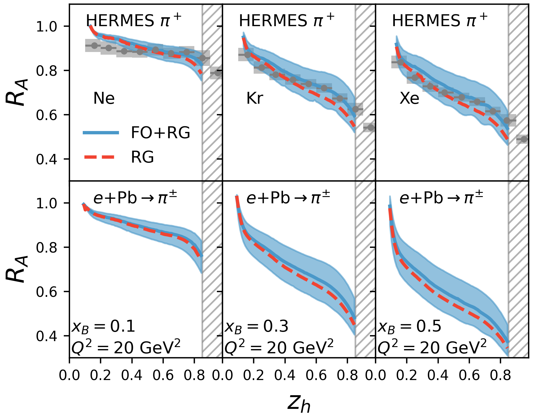
Figure 1: Top panel: medium modifications to the $\pi^{+}$ fragmentation function compare to HERMES data, performed for the average $\nu=12$ GeV, $Q^{2}=2.25$ GeV². Bottom panel: predictions for the modified pion fragmentation function at EIC with Pb nucleus for three $(x_{B},Q^{2})$ combinations.

We demonstrate the new method by studying nuclear effects on pion fragmentation in SIDIS, with the cross section given in Eq. (2). We implement the fully-coupled RG evolution Eqs. (12), (13), (14), and the fixed order terms in Eq. (11). The nuclear modifications is defined as the ratio of inclusive-normalized cross sections between electron-nucleus ($e$A) and electron-deuterium ($ed$ for HERMES) or electron-proton ($ep$ for EIC) collisions

$$R_{A}(x_{B},Q^{2},z_{h})=\frac{\frac{d\sigma_{eA\rightarrow h}}{dx_{B}dQ^{2}dz_{h}}/\frac{d\sigma_{eA}}{dx_{B}dQ^{2}}}{\frac{d\sigma_{ed,ep\rightarrow h}}{dx_{B}dQ^{2}dz_{h}}/\frac{d\sigma_{ed,ep}}{dx_{B}dQ^{2}}}\,.\;\;$$ (19)

For parton distribution and fragmentation functions we use the nNNPDF30nlo Khalek et al. (2022) and NNFF10lo parametrizations Bertone et al. (2017) and perform the calculation for the averaged HERMES kinematics $Q^{2}=2.25$ GeV² and $\nu=12$ GeV Airapetian et al. (2007). To numerically solve Eqs. (12) and (14), we smear the singular hard parton energy spectrum by a Gaussian with width parameter $\sigma_{z}=0.05$ and the evolution from $\mu_{1}=Q$ to $Q_{0}=1$ GeV is performed using standard vacuum DGLAP. In turn, the in-medium RG evolves $\mu_{2}^{2}$ from $\chi(w_{\rm max})z\nu/L$ to $\mu_{D}^{2}$. We take $\Lambda_{\rm QCD}=0.16$ GeV, the inverse range of the interaction $\mu_{D}^{2}=0.12$ GeV² and the central value of the effective medium density parameter $\rho_{G}=0.4\;{\rm fm}^{-3}$. These values yield a quark transport parameter $\hat{q}_{F}\approx 0.053$ GeV²/fm at $\nu=12$ GeV (see supplemental material), consistent with existing mDGLAP applications Li and Vitev (2021); Li et al. (2021). An average over the geometry of the nucleus of radius $r_{A}=1.2A^{1/3}$ fm is also performed.

The resulting nuclear modification factor $R_{A}(z_{h})$ is compared to the HERMES data for ²⁰Ne and ¹³¹Xe targets Airapetian et al. (2007) in the top row of Fig. 1. Qualitatively, in-medium evolution shifts hadron spectra towards lower $z_{h}$. Results including only RG contributions (red dashed lines) give a good description of $R_{A}$ from small to intermediate $z$, but lead to a suppression that is too strong at large $z_{h}$. We remark that the region very close to $z_{h}=1$ is dominated by soft emissions, where one should consider soft power counting and threshold type resummation in both vacuum Catani and Trentadue (1989); Anderle et al. (2013) and in-medium calculations. Therefore, we have exclude this region from our comparison. Blue solid lines include the fixed order (FO) contribution from Eq. (10) in the initial condition of the RG evolution, and the bands correspond to the density variation in the range $(\rho_{G}/1.5,1.5\rho_{G})$. The FO correction improves the description of HERMES data at large $z$, but remains subleading to the RG evolution effect. The nuclear size dependence of $R_{A}$ for Ne, Kr, and Xe nuclei is naturally explained with the same set of transport parameters.

Using the same in-medium transport parameters, we present projections (lower panel of Fig. 1) for modified pion fragmentation functions at the future electron-ion collider (EIC) for $e$Pb reactions at fixed $Q^{2}=20$ GeV² and various Bjorken $x_{B}$ values. We find that for $x_{B}>0.3$, where partons are less energetic in the nuclear rest frame, modifications become very large, consistent with existing predictions for heavy flavor and jets Li et al. (2021); Li and Vitev (2021).

Summary.  In the limit $Q/Q_{0},E/(\mu_{D}^{2}L),\lambda_{g}\mu_{D}\gg 1$ and to first order in the opacity of QCD matter we performed a renormalization group (RG) analysis of medium effects for the SIDIS process on a nuclear target. We derived a set of in-medium RG equations that resum the leading $\ln[E/(\mu_{D}^{2}L)]$ terms from multiple medium-induced emissions and identified the corresponding fixed order corrections. We further showed that such resummation is also contained in the modified DGLAP equations, which differ in the way of regulating the endpoint divergences of medium-induced emission spectra. Importantly, the new RG evolution in matter approach provides analytic insight into the salient features of parton showers responsible for the modification of hadron production in $eA$ that are not possible with numerical methods alone. It is a more efficient and systematically improvable way of treating the logarithmic enhancements in matter as compared to solving mDGLAP.

We applied the new method to study the cold nuclear matter (CNM) effects on pion fragmentation and found that it gives a good description of the HERMES SIDIS data. Predictions for the future EIC were also presented, where improved theoretical precision is especially important Abdul Khalek et al. (2022). The semi-analytic framework derived here can be generalized to initial-state CNM effects, such as the ones observed in Drell-Yan production in proton-nucleus collisions, and to heavy ion collisions. This work further benefits future QCD studies by providing guidance on incorporating medium effects in Monte-Carlo event generators for the EIC, the Relativistic Heavy Ion Collider and the Large Hadron Collider.

Acknowledgments.— The authors would like to thank Duff Neill for helpful discussion. This work is supported by the U.S. Department of Energy, Office of Science, Office of Nuclear Physics through Contract No. 89233218CNA000001 and by the Laboratory Directed Research and Development Program at LANL.

I Supplementary Material

I.1 In-medium scattering cross section and jet transport parameter estimate

The elastic cross section between jet and target partons in color representations $R$ and $T$, respectively, is Ovanesyan and Vitev (2011)

$$\frac{d\sigma_{TR}}{d^{2}\mathbf{q}}=\frac{1}{(2\pi)^{2}}\frac{1}{d_{A}}\frac{4\pi\alpha_{s}C_{T}\times 4\pi\alpha_{s}C_{R}}{(\mathbf{q}^{2}+\mu_{D}^{2})^{2}}\,,$$ (20)

with $d_{A}=N_{c}^{2}-1$. The collision rate after summing over the medium color sources of representation $T$ with density $\rho_{T}$ then reads

$$\sum_{T}\rho_{T}\frac{d\sigma_{TR}}{d^{2}\mathbf{q}}=\sum_{T}\frac{1}{(2\pi)^{2}}\frac{\rho_{T}}{d_{A}}\frac{4\pi\alpha_{s}C_{T}\times 4\pi\alpha_{s}C_{R}}{(\mathbf{q}^{2}+\mu_{D}^{2})^{2}}=\frac{\alpha_{s}C_{R}}{\pi}\frac{1}{(\mathbf{q}^{2}+\mu_{D}^{2})^{2}}\rho_{G}\,,\quad\rho_{G}\equiv\sum_{T}\rho_{T}\frac{4\pi\alpha_{s}^{\rm med}C_{T}}{d_{A}}\,.\;$$ (21)

In other words, we have chosen to put kinematic factors, the square color charges and coupling to the medium in the effective medium gluon density $\rho_{G}$. With $\mu_{D}^{2}=0.12$ GeV², $\rho_{G}=0.4$ fm^-3, the quark jet transport parameter is

$$\hat{q}_{F} = \int_{0}^{\mathbf{q}_{\rm max}^{2}=\nu\mu_{D}/2}d^{2}\mathbf{q}\,\mathbf{q}^{2}\frac{\alpha_{s}C_{F}}{\pi}\frac{1}{(\mathbf{q}^{2}+\mu_{D}^{2})^{2}}\rho_{G}\,\approx 0.053~{}\mathrm{GeV}^{2}/\mathrm{fm}$$ (22)

for $\nu=Q^{2}/(2x_{B}M_{p})=12$ GeV in the nuclear rest frame. Here, the ultraviolet cut off of the $\mathbf{q}^{2}$ integration is chosen to be $\nu\mu_{D}/2$, as in Ref. Vitev (2007). The running coupling is cut-off when $\alpha_{s}$ reaches $2\pi/\beta_{0}$.The value of $\hat{q}$ is further consistent with the analysis of Li et al. (2021); Li and Vitev (2021).

I.2 Full splitting functions in matter

The splitting functions in nuclear matter induced by final-state interactions are taken from Refs. Ovanesyan and Vitev (2011); Kang et al. (2017) (in $d=4$ dimension). After performing the path length integration in a medium of uniform density and size $L$, the splitting functions become

$$P_{ij}^{(1)}(x) = \frac{\alpha_{s}}{2\pi^{2}}P_{ij}(x)L\int d^{2}\mathbf{k}\sum_{T}\int\frac{d^{2}\mathbf{q}}{(2\pi)^{2}}\frac{\rho_{T}}{d_{A}}\frac{4\pi\alpha_{s}C_{T}\times 4\pi\alpha_{s}}{(\mathbf{q}^{2}+\mu_{D}^{2})^{2}}W_{ij}(x,\mathbf{k},\mathbf{q},E/L)$$ (23)

$$\equiv \frac{\alpha_{s}}{2\pi^{2}}P_{ij}(x)L\int d^{2}\mathbf{k}\int\frac{d^{2}\mathbf{q}}{(2\pi)^{2}}\frac{\rho_{G}\times 4\pi\alpha_{s}}{(\mathbf{q}^{2}+\mu_{D}^{2})^{2}}W_{ij}(x,\mathbf{k},\mathbf{q},E/L)\,.$$

The continuous parts of the vacuum splitting functions in $d=4-2\epsilon$ dimension, arising from real emissions, are

$$P_{qq}(x)=C_{F}\left[\frac{1+x^{2}}{1-x}-\epsilon(1-x)\right],~{}P_{gq}(x)=T_{R}[x^{2}+(1-x)^{2}-2\epsilon x(1-x)],$$ (24)

$$P_{qg}(x)=P_{qq}(1-x),~{}P_{gg}(x)=C_{A}\frac{1+x^{4}+(1-x)^{4}}{x(1-x)}\,.\;\;$$ (25)

The diagonal terms also receive virtual corrections, which we determined from flavor and momentum sum rules Chien et al. (2016).

For $P_{ij}^{(1)}(x)$, we define $\mathbf{A}_{\perp}=\mathbf{k},~{}\mathbf{B}_{\perp}=\mathbf{k}+(1-x)\mathbf{q},~{}\mathbf{C}_{\perp}=\mathbf{k}-x\mathbf{q},~{}\mathbf{D}_{\perp}=\mathbf{k}+\mathbf{q}$, and interference phase factors

$$\Phi_{A}=\Phi\left[\frac{\mathbf{A}_{\perp}^{2}L}{2x(1-x)E}\right],~{}\Phi_{B}=\Phi\left[\frac{\mathbf{B}_{\perp}^{2}L}{2x(1-x)E}\right],~{}\Phi_{C}=\Phi\left[\frac{\mathbf{C}_{\perp}^{2}L}{2x(1-x)E}\right],$$

$$~{}\Phi_{AD}=\Phi\left[\frac{(\mathbf{A}_{\perp}^{2}-\mathbf{D}_{\perp}^{2})L}{2x(1-x)E}\right],~{}\Phi_{CB}=\Phi\left[\frac{(\mathbf{C}_{\perp}^{2}-\mathbf{B}_{\perp}^{2})L}{2x(1-x)E}\right]\,.$$ (26)

Then, $W_{ij}$, including the relevant quadratic Casimirs from the Glauber gluon–hard parton system interactions, are

$$W_{qq} = C_{A}\frac{\mathbf{B}_{\perp}}{\mathbf{B}_{\perp}^{2}}\left(\frac{\mathbf{B}_{\perp}}{\mathbf{B}_{\perp}^{2}}-\frac{\mathbf{A}_{\perp}}{\mathbf{A}_{\perp}^{2}}\right)\Phi_{B}+C_{A}\frac{\mathbf{B}_{\perp}}{\mathbf{B}_{\perp}^{2}}\left(\frac{\mathbf{B}_{\perp}}{\mathbf{B}_{\perp}^{2}}-\frac{\mathbf{C}_{\perp}}{\mathbf{C}_{\perp}^{2}}\right)\Phi_{B}+(2C_{F}-C_{A})\frac{\mathbf{C}_{\perp}}{\mathbf{C}_{\perp}^{2}}\left(\frac{\mathbf{C}_{\perp}}{\mathbf{C}_{\perp}^{2}}-\frac{\mathbf{A}_{\perp}}{\mathbf{A}_{\perp}^{2}}\right)\Phi_{C}+C_{A}\Delta W\,,$$ (27)

$$W_{gg} = C_{A}\frac{\mathbf{B}_{\perp}}{\mathbf{B}_{\perp}^{2}}\left(\frac{\mathbf{B}_{\perp}}{\mathbf{B}_{\perp}^{2}}-\frac{\mathbf{A}_{\perp}}{\mathbf{A}_{\perp}^{2}}\right)\Phi_{B}+C_{A}\frac{\mathbf{B}_{\perp}}{\mathbf{B}_{\perp}^{2}}\left(\frac{\mathbf{B}_{\perp}}{\mathbf{B}_{\perp}^{2}}-\frac{\mathbf{C}_{\perp}}{\mathbf{C}_{\perp}^{2}}\right)\Phi_{B}+C_{A}\frac{\mathbf{C}_{\perp}}{\mathbf{C}_{\perp}^{2}}\left(\frac{\mathbf{C}_{\perp}}{\mathbf{C}_{\perp}^{2}}-\frac{\mathbf{A}_{\perp}}{\mathbf{A}_{\perp}^{2}}\right)\Phi_{C}+C_{A}\Delta W\,,$$ (28)

$$W_{gq} = C_{A}\frac{\mathbf{B}_{\perp}}{\mathbf{B}_{\perp}^{2}}\left(\frac{\mathbf{B}_{\perp}}{\mathbf{B}_{\perp}^{2}}-\frac{\mathbf{A}_{\perp}}{\mathbf{A}_{\perp}^{2}}\right)\Phi_{B}+(2C_{F}-C_{A})\frac{\mathbf{B}_{\perp}}{\mathbf{B}_{\perp}^{2}}\left(\frac{\mathbf{B}_{\perp}}{\mathbf{B}_{\perp}^{2}}-\frac{\mathbf{C}_{\perp}}{\mathbf{C}_{\perp}^{2}}\right)\Phi_{B}+C_{A}\frac{\mathbf{C}_{\perp}}{\mathbf{C}_{\perp}^{2}}\left(\frac{\mathbf{C}_{\perp}}{\mathbf{C}_{\perp}^{2}}-\frac{\mathbf{A}_{\perp}}{\mathbf{A}_{\perp}^{2}}\right)\Phi_{C}+(2C_{F}-C_{A})\Delta W,~{}~{}~{}~{}~{}~{}$$ (29)

and $W_{qg}=W_{qq}(x\rightarrow 1-x)$. For each channel, the first three terms can be cast into the form of the first line of Eq. (6) by shifting integration variables such that arguments of $\Phi(\cdot)$ become $\mathbf{k}^{2}L/[2x(1-x)E]$. The remaining piece $\Delta W$,

$$\Delta W = \left[\frac{\mathbf{C}_{\perp}}{\mathbf{C}_{\perp}^{2}}\left(\frac{\mathbf{C}_{\perp}}{\mathbf{C}_{\perp}^{2}}-\frac{\mathbf{B}_{\perp}}{\mathbf{B}_{\perp}^{2}}\right)\Phi_{C}+\frac{\mathbf{B}_{\perp}}{\mathbf{B}_{\perp}^{2}}\cdot\frac{\mathbf{C}_{\perp}}{\mathbf{C}_{\perp}^{2}}\Phi_{CB}\right]-\left[\frac{\mathbf{A}_{\perp}}{\mathbf{A}_{\perp}^{2}}\left(\frac{\mathbf{A}_{\perp}}{\mathbf{A}_{\perp}^{2}}-\frac{\mathbf{D}_{\perp}}{\mathbf{D}_{\perp}^{2}}\right)\Phi_{A}+\frac{\mathbf{A}_{\perp}}{\mathbf{A}_{\perp}^{2}}\cdot\frac{\mathbf{D}_{\perp}}{\mathbf{D}_{\perp}^{2}}\Phi_{AD}\right]\,,$$ (30)

is written as the difference of two terms. Note that the second term can be obtained from the first one by shifting $\mathbf{k}\rightarrow\mathbf{k}+x\mathbf{q}$, causing $\mathbf{C}_{\perp}\rightarrow\mathbf{A}_{\perp}$ and $\mathbf{B}_{\perp}\rightarrow\mathbf{D}_{\perp}$. Therefore, $\Delta W=0$ under dimensional regularized integration of $\mathbf{k}$ and $\mathbf{q}$. If one uses an explicit ultraviolet cut-off $\Lambda_{\rm UV}$, the integration of $\Delta W$ over $\mathbf{q},\mathbf{k}$ (or in general, any differences caused by a shift of $\mathbf{k}+\Delta\cdot\mathbf{q}$ of Eqs. (27),(28), and (29)) are further suppressed by $\Lambda_{\rm UV}^{-2}$ and do not contribute to the medium-induced logarithmic enhancement.

We can account for the virtuality of the collision Eq. (6) by introducing the variable $w_{\rm max}=Q^{2}L/(2\nu)$, which appears in the functions $B$ and $\chi$ defined as

$$B(w_{\rm max})=\frac{4}{\pi}\int_{0}^{w_{\rm max}}\Phi(x)\frac{dx}{x^{2}},~{}~{}~{}\chi(w_{\rm max})=2\exp\left\{\frac{1}{B(w_{\rm max})}\frac{4}{\pi}\int_{0}^{w_{\rm max}}\Phi(x)\ln(x)\frac{dx}{x^{2}}+\gamma_{E}\left(\frac{1}{B(w_{\rm max})}-1\right)\right\}.\;\;$$ (31)

For the SIDIS process at moderate $x_{B}$, $w_{\rm max}\equiv x_{B}M_{p}L\approx 6.0x_{B}A^{1/3}$ is of order few. For fragmentation at mid rapidity in hadronic collisions, $Q^{2}L/(2E)\sim EL\rightarrow\infty$, and $B(\infty)=1$, $\chi(\infty)=2e^{3/2-\gamma_{E}}\approx 5.0$.

I.3 The flavor singlet sector

Analogously to the treatment of the flavor non-singlet sector, we provide the details for the subtraction of divergences and renormalization of the flavor singlet sector. To isolate the extra $[x(1-x)]^{-1-2\epsilon}$ poles, we define the following decomposition for any well-behaved function $G(x)$. For singularities associate to $P^{(1)}_{qg}(x)$,

$$\int_{0}^{1}\frac{G(x)}{x^{2+2\epsilon}(1-x)^{1+2\epsilon}}dx = \int_{0}^{1}\frac{\left\{G(x)\right\}_{qg}}{x^{2}(1-x)}dx-\frac{G(0)}{2\epsilon}-\frac{G^{\prime}(0)}{2\epsilon}-G(1)\left(\frac{1}{2\epsilon}+2\right)+\mathcal{O}(\epsilon)\,,$$ (32)

with $\left\{G(x)\right\}_{qg}=G(x)-x^{2}G(1)-(1-x^{2})G(0)-x(1-x)G^{\prime}(0)$. For singularities associate to $P^{(1)}_{gg}(x)$,

$$\int_{0}^{1}\frac{G(x)}{x^{2+2\epsilon}(1-x)^{2+2\epsilon}}dx = \int_{0}^{1}\frac{\left\{G(x)\right\}_{gg}}{x^{2}(1-x)^{2}}dx-G(0)\left[\frac{1}{\epsilon}+2\right]-\frac{G^{\prime}(0)}{2\epsilon}-G(1)\left[\frac{1}{\epsilon}+2\right]+\frac{G^{\prime}(1)}{2\epsilon}+\mathcal{O}(\epsilon)\,,$$ (33)

with $\left\{G(x)\right\}_{gg}=G(x)-(1-x)^{2}\left[(1+2x)G(0)+xG^{\prime}(0)\right]-x^{2}\left[(3-2x)G(1)+(x-1)G^{\prime}(1)\right]$. Finally, for $P^{(1)}_{gq}(x)$

$$\int_{0}^{1}\frac{G(x)}{x^{1+2\epsilon}(1-x)^{1+2\epsilon}}dx = \int_{0}^{1}\frac{\left\{G(x)\right\}_{gq}}{x(1-x)}dx-\frac{G(0)}{2\epsilon}-\frac{G(1)}{2\epsilon}+\mathcal{O}(\epsilon)\,,$$ (34)

with $\left\{G(x)\right\}_{gq}=G(x)-xG(1)-(1-x)G(0)$. One can directly and explicitly check that the endpoint divergences are removed from the integration. With this procedure, the medium-induced NLO contributions from these channels can be decomposed into log-enhanced and fixed order contributions,

$$\frac{\Delta F_{g}}{A(\mu_{2}^{2},E,w_{\rm max})}=\left(\frac{1}{2\epsilon}+\mathcal{L}\right)\left[-4C_{A}^{2}\frac{dF_{g}(z)}{dz}+2C_{F}N_{f}\frac{F_{g}(z)}{z}-2C_{F}^{2}\sum_{f}\frac{F_{f}(z)}{z}\right]$$ (35)

$$+ \sum_{f}\int_{0}^{1}dx\frac{\left\{\sum_{n}C_{n}^{qg}\left(\Delta_{n}^{qg}\right)^{2}C_{F}[1+(1-x)^{2}]\frac{x}{z}F_{f}(\frac{z}{x})\right\}_{qg}}{x^{2}(1-x)}-N_{f}\frac{F_{g}(z)}{z}\int_{0}^{1}dx\frac{\left\{\sum_{i}C_{n}^{gq}\left(\Delta_{n}^{gq}\right)^{2}T_{R}[x^{2}+(1-x)^{2}]\right\}_{gq}}{x(1-x)}$$

$$+ \int_{0}^{1}dx\frac{\left\{\sum_{i}C_{n}^{gg}\left(\Delta_{n}^{gg}\right)^{2}C_{A}[1+x^{4}+(1-x)^{4}]\left[\frac{x}{z}F_{g}(\frac{z}{x})-x\frac{F_{g}(z)}{z}\right]\right\}_{gg}}{x^{2}(1-x)^{2}}+14C_{A}^{2}\frac{F_{g}(z)}{z}-3C_{F}^{2}\sum_{f}\frac{F_{f}(z)}{z}\,,\;\;\;$$

$$\frac{\Delta F_{f}}{A(\mu_{2}^{2},E,w_{\rm max})} = \left(\frac{1}{2\epsilon}+\mathcal{L}\right)\left[-4C_{F}C_{A}\frac{dF_{f}(z)}{dz}+2C_{F}(2C_{A}+C_{F})\frac{F_{f}(z)}{z}-C_{F}\frac{F_{g}(z)}{z}\right]$$ (36)

$$+ \int_{0}^{1}\frac{\left\{\sum_{n}C_{n}\Delta_{n}^{2}(x)C_{F}(1+x^{2})\left(\frac{x}{z}F_{f}\left(\frac{z}{x}\right)-\frac{F_{f}(z)}{z}\right)\right\}_{qq}}{x(1-x)^{2}}dx+(4C_{A}-C_{F})C_{F}\frac{F_{f}(z)}{z}$$

$$+ \int_{0}^{1}dx\frac{\left\{\sum_{i}C_{n}^{gq}\left(\Delta_{n}^{gq}\right)^{2}T_{R}[x^{2}+(1-x)^{2}]\frac{x}{z}F_{g}(\frac{z}{x})\right\}_{gq}}{x(1-x)}\,,\;\;$$

where $\mathcal{L}\equiv\ln\frac{\mu_{2}^{2}}{\chi E/L}$ and $\left\{\cdots\right\}_{ij}$ stands for the subtraction for the corresponding channel $i\rightarrow j$. The $1/\epsilon$ poles are subtracted by the corresponding contribution from $M_{ij}^{(1)}$. Then, taking derivatives with respect to $\tau$ gives the in-medium RG Eqs. (13) and (14) for the flavor singlet sector.